Development of Rural Bicycle Compatibility Index

Transcription

1 University of Nebraska - Lincoln DigitalCommons@University of Nebraska - Lincoln Nebraska Department of Transportation Research Reports Nebraska LTAP Development of Rural Bicycle Compatibility Index Elizabeth G. Jones University of Nebraska-Lincoln, libby.jones@unl.edu Follow this and additional works at: Part of the Transportation Engineering Commons Jones, Elizabeth G., "Development of Rural Bicycle Compatibility Index" (2004). Nebraska Department of Transportation Research Reports This Article is brought to you for free and open access by the Nebraska LTAP at DigitalCommons@University of Nebraska - Lincoln. It has been accepted for inclusion in Nebraska Department of Transportation Research Reports by an authorized administrator of DigitalCommons@University of Nebraska - Lincoln.

2 TOC NDOR Research Project Number SPR-PL-1(038) P533 Transportation Research Studies FINAL REPORT DEVELOPMENT OF RURAL BICYCLE COMPATIBILITY INDEX Elizabeth G. Jones, Ph.D. Department of Civil Engineering College of Engineering and Technology 203E PKI Building 6001 Dodge Street Omaha, NE Telephone (402) FAX (402) Sponsored by the Nebraska Department of Roads 1500 Nebraska Highway 2 Lincoln, NE Telephone (402) FAX (402) July 2004

3

4 TECHNICAL REPORT STANDARD TITLE PAGE 1. Report No. 2. Government Accession No 3. Recipient s Catalog No 4. Title and Subtitle Development of Rural Bicycle Compatibility Index 7. Authors Elizabeth G. Jones 9. Performing Organization Name and Address Department of Civil Engineering University of Nebraska-Lincoln 203E PKI Building 6001 Dodge Street Omaha, NE Sponsoring Agency Name and Address Nebraska Department of Roads 1500 Nebraska Highway 2 Lincoln, NE Report Date July Performing Organization Code 8. Performing Organization Report No. 10. Work Unit No. (TRAIS) 11. Work Unit No. SPR-PL-1(038) P Type of Report and Period Covered Final Report 14. Sponsoring Agency Code 15. Supplementary Notes 16. Abstract Level of Service (LOS) is a qualitative measure that describes the operation of motor vehicle traffic. LOS is defined using traffic characteristics such as speed, travel time, freedom to maneuver, and safety. A standard system for measuring Level of Service has been in use for many years in the description of motor vehicle traffic. In the area of bicycle transportation, no such standard currently exists. Many attempts at developing a LOS standard have been made for describing urban traffic, but no research has specifically focused on describing rural bicycle traffic. The development of a rural bicycle compatibility index (RBCI) is described. A recent Federal Highway Administration (FHWA) research project developed a Bicycle Compatibility Index (BCI). This index was developed for urban and suburban roadway segments and incorporated those variables that bicyclists typically use to assess how compatible a roadway segment is for travel by bicycle. The FHWA BCI can be used by bicycle coordinators, transportation planners, traffic engineers, and others to evaluate existing facilities to determine what improvements may be required, as well as the geometric and operational requirements for new facilities to achieve the desired level of bicycle service. The objective of this thesis is to develop a rural equivalent of the BCI. Roadways in rural Nebraska were used to develop the RBCI. Although the specific results of this work are clearly applicable to Nebraska and other similar rural areas, the general methodology and concepts could easily be used to develop a more general RBCI that would have national applicability. An RBCI will provide bicycle coordinators, transportation planners, traffic engineers, and others the capability to better plan and design bicycle compatible roadways. Specifically, an RBCI model can be used for operational evaluation, design, and planning. 17. Key Words 18. Distribution Statement No restriction. This document is available to the public from the sponsoring agency. 19. Security Classif.(of this report) Unclassified Form DOT (8-72) 20. Security Classif. (of this page) Unclassified 21. No. of Pages 22. Price i

5 DISCLAIMER This research was funded through the Nebraska Department of Roads Research Program and the Federal Highway Administration under Project SPL-PL-1(038) P533. The contents of this report reflect the views of the authors who are responsible for the facts and the accuracy of the data presented herein. The contents do not necessarily reflect the official views of the Nebraska Department of Roads, the Federal Highway Administration, or the University of Nebraska- Lincoln at the time of publication. This document is disseminated under the sponsorship of the Department of Transportation in the interest of information exchange. The United States Government assumes no liability for its contents or use thereof. This report does not constitute a standard, specification or regulation. The United State Government and the State of Nebraska do not endorse products or manufacturers. Trade and manufacturers names appear in this report only because they are considered essential to the object of the document. ii

6 TABLE OF CONTENTS TECHNICAL REPORT STANDARD TITLE PAGE i DISCLAIMER ii TABLE OF CONTENTS iii LIST OF FIGURES iv LIST OF TABLES v 1 Introduction GENERAL PROBLEM STATEMENT LITERATURE REVIEW FORMAL PROBLEM STATEMENT 16 2 Research Methodology EXPERIMENTAL DESIGN SITE SELECTION VIDEO COLLECTION DATA COLLECTION VIDEOTAPE ANALYSIS AND SELECTION VIDEO COMPRESSION WEB-SURVEY DEVELOPMENT VIDEO SURVEY PROCESS 34 3 Data Analysis ANALYSIS OF SURVEY RESPONSES DESCRIPTIVE STATISTICS FOR THE SURVEY RESULTS 41 4 Regression analysis to develop the rural bicycle compatibility index REGRESSION ANALYSIS FINAL REGRESSION MODEL COMPARISON OF RATINGS TESTING RBCI WITH SAMPLE POINTS 67 5 Implementation of the RBCI INITIAL IMPLEMENTATION MAP DEVELOPMENT IMPLEMENTATION CHALLENGES PRESENTATION OF INITIAL MAP FINAL PRESENTATION OF MAP COMPARING THE BICYCLE GUIDE MAP AND THE RBCI MAP 80 6 Summary and Conclusions STRENGTHS OF THE RESEARCH LIMITATIONS OF THE RESEARCH CONCLUSIONS 83 REFERENCES 85 Appendix A 87 Appendix B 94 Appendix C 135 iii

7 LIST OF FIGURES FIGURE NDOR Bicycle Guide Map 2 FIGURE 2 Camera mounting system. (a) Side view. (b) Front view. 22 FIGURE 3 Recording vehicle position and observed movement of passing vehicles on roadways with (a) Shoulder and (b) No shoulder. 23 FIGURE 4 Sample data collection form used to record characteristics of roadway segments 26 FIGURE 5 Sample picture of video clips. (a) Uncompressed. (b) Compressed. 29 FIGURE 6 Typical video survey page 33 FIGURE 7 Comparison of mean comfort level ratings 64 FIGURE 8 Comparison of survey response average and computed RBCI and BCI ratings 65 FIGURE 9 GIS map showing the highway routes mapped in the shoulder width shapefile. 70 FIGURE 10 GIS map showing the highway routes mapped in the truck count shapefile. 71 FIGURE 11 Map of Nebraska cities considered urban areas in RBCI map development. 72 FIGURE 12 Final draft of the RBCI map 79 iv

8 LIST OF TABLES TABLE 1 Relationship between LOS and BCI 7 TABLE 2 Experimental design 19 TABLE 3 Potential data collection locations with AADT and heavy vehicle volumes 21 TABLE 4 Data collection locations 25 TABLE 5 Experimental design with segment numbers used for video clips 33 TABLE 6 Sample size determination 35 TABLE 7 Determination of bicycling experience 37 TABLE 8 Survey participant characteristics 39 TABLE 9 Sample size statistics for 90% confidence interval 40 TABLE 10 Sample size statistics for 95% confidence interval 40 TABLE 11 Summary of actual sample statistics 40 TABLE 12 Comparison of mean survey responses to responses of subject with lowest comfort rating 42 TABLE 13 Comparison of mean survey responses to responses of subject with highest comfort rating 43 TABLE 14 Summary of response variability 44 TABLE 15 Independent variables used in regression analyses 46 TABLE 16 Comparison of regression models 1, 2, and 3 47 TABLE 17 Comparison of regression models 4, 5 and 6 52 TABLE 18 Comparison of regression models 7, 8 and 9 55 TABLE 19 Comparison of regression models 10, 11 and TABLE 20 Comparison of regression Models 13, 14, and TABLE 21 Comparison of RBCI and BCI 66 TABLE 22 Directional distribution of heavy vehicle traffic on rural highways in Nebraska 73 v

9 1 INTRODUCTION 1.1 General Problem Statement Bicycles have served as a mode of transportation for over 100 years. Their involvement in the transportation infrastructure over this period of time started as a new form of primary transportation, changed to a mostly recreational form of transportation, and today bicycles are being utilized for both purposes. In an attempt to expand the modes of transportation used in day to day life, the United States Congress passed the Intermodal Surface Transportation Efficiency Act (ISTEA) in This act provided for a significant amount of funding for modes of transportation not greatly utilized up to that point in time. With the passage of this legislation, consideration of the bicycle in statewide transportation planning became a requirement for all states. In its efforts to comply with ISTEA, and followed by TEA-21, the Nebraska Department of Roads (NDOR) produced a Bicycle Guide Map. This map provides cyclists with information such as the existence of a shoulder on a given stretch of highway, the general amount of traffic on a road, the classification of the road (Federal, State, or County), and the daily amount of heavy vehicle traffic carried by a particular roadway. This map gives cyclists a general idea of the characteristics of a highway section and provides helpful information to a cyclist in the selection of cycling routes through the state. Although this map is helpful, it requires the cyclist to synthesize the information to determine how compatible a roadway may be for bicycling. The Bicycle Guide Map for Nebraska is shown in Figure 1. To improve the clarity of the Bicycle Guide Map, the NDOR asked the University of Nebraska- Lincoln to develop a method for assisting bicyclists in the synthesis of the information regarding the compatibility of roadways for bicycling. The result of the research for this project is the Rural Bicycle Compatibility Index (RBCI). The RBCI is a scientifically developed method for determining the suitability of a roadway for bicycle use. The methodology used to develop the RBCI was adapted from the methodology used to develop the Bicycle Compatibility Index (BCI). The BCI is a method for determining the usability of urban and suburban streets for bicycle use. The research used to develop the BCI was conducted by the University of North Carolina (UNC) and was sponsored by the Federal Highway Administration (FHWA). (1,2) In their research, the UNC research team collected data from selected roadways, created a survey using video taken from the selected sites, surveyed a group of people, and then used the results of this survey to develop a linear regression model to generate an index that would rate roadways for their suitability for bicycle use. A very similar model was used to develop the RBCI. 1

10 FIGURE NDOR Bicycle Guide Map 2

11 The goals in developing the RBCI were based on the desire to make choice of route through the State of Nebraska a simpler process for bicyclists. Three goals were identified for the development of the RBCI: 1. Develop a model for bicyclists to easily evaluate rural highways for bicycle use. 2. Develop a standard method of study for other states to evaluate their own rural highways for bicycle ridership. 3. Update the NDOR Bicycle Guide Map using the RBCI developed for Nebraska. Development of the RBCI has come about in part using the body of research that has sought to develop a method of rating roadways for bicycle use. A review of this research is included to gain an understanding of the history and progress of rating methodologies. 1.2 Literature Review Over the past decade, more attention has been paid to the needs of bicyclists in transportation planning efforts. Action taken by the United States Congress in 1991 with the passage of the Intermodal Surface Transportation Efficiency Act (ISTEA) has provided for additional funding throughout the country for research into modes of transportation other the motor vehicle traffic. With this additional funding there has been an increase in research relating to the needs of bicyclists. The most groundbreaking study of Bicycle LOS compatibility was the Geelong Bikeplan. The concept of the compatibility of a roadway for bicyclists is important in that it is based on a bicyclist s perspective of geometric and traffic conditions for a particular segment of road. The evolution of this concept began with work in 1978 by the Geelong Bikeplan Team in Australia (3). This team used a concept of bicycle stress level to account for the perspective of a bicyclist regarding roadway suitability for bicycling. The bicycle stress level concept assumes that bicyclists want to minimize not only the physical effort required to ride a bicycle, but also the mental effort needed to safely negotiate the geometry and traffic operations of a roadway. The Geelong Bikeplan Team used their bicycling experience to rate the stress caused by three variables curb lane width, motor vehicle speed, and traffic volume believed by the team to most significantly affect bicycling stress. The Davis Bicycle Safety Index Rating (BSIR) (4) is a method for measuring the condition of roadways for bicycle use. It included a Roadway Segment Index (RSI) that was a number that represented the combined factors of average daily traffic (ADT), number of traffic lanes, speed limit, width of the outside traffic lane, sum of pavement factors, and the sum of location factors. Davis also included an Intersection Evaluation Index (IEI) to analyze riding conditions through intersections. (4) The importance of this research was the identification of per-lane traffic volume, traffic speed, and lane width as the main factors that affect a bicyclist s perception of riding conditions. Epperson (5) summarized a number of bicycle level of service models and also suggested other possible methods of study that may be effective in the study of bicycle stress indicators and bicycle level of service models. Epperson suggested that destination surveys be given to bicyclists arriving at various sites to determine how routes may have been selected and how 3

12 conditions on those routes led the cyclists to choose them. (5) Additionally, it was suggested that videotapes of road segments be used as a method of analysis. The recorded segments could then be rated by large groups of people. The videotaping method would be inexpensive and useful in comparing an overall roadway index for a road segment with cylists perceptions. (5) Sorton and Walsh (6) used the concept of the bicycle stress level and expanded upon the Geelong work by including the perspectives of bicyclists other than the research team members. However, no additional variables that may have an effect on the bicycle stress level were included. Sorton and Walsh also used videotape to assist in this effort and were able to show that bicyclists can recognize differences in the three variables and that these differences are consistently reflected in their stress level ratings. These three variables included curb lane traffic volume, speed of motor vehicles, and curb lane width. In addition to testing the three primary variables, secondary variables such as, commercial driveways per mile along a street, parking turnover, and percentage of heavy vehicles using the road, (6) were suggested as variables that may have an impact on bicyclists using a given roadway. Sorton and Walsh categorized their research participants into three categories: youth, casual, and experienced. (6) These three categories of riders were based on responses to questions that surveyed the number of miles ridden in a week, type of street used while riding, and frequency of riding. Experienced riders rode more than 20 miles per week, rode frequently, rode on arterial streets, and commuted regularly. Casual riders did not ride on arterial streets, used their bicycles as a form of recreation, rode infrequently, used sidewalks, and rode less than 5 miles per week. Youth bicyclists were those cyclists aged between 10 and 15 years of age. (6) This research was important in the development of procedures to evaluate stress levels felt by bicyclists. In addition to the importance of developing evaluative procedures for different traffic and geometric conditions, the research also came up with some important conclusions about the results that were obtained. It concluded that bicyclists can recognize the variations in different traffic and geometric conditions and also that bicyclists perceive variations in the form of stress level. (6) A model for measuring bicyclists perception of roadway hazards was developed by Landis. (7) The model, called the bicycle Interaction Hazard Score (IHS), uses the input of eight variables into the model equation. The model used such inputs as average daily traffic (ADT), total number of through lanes, commercial or non-commercial land use in the surrounding area, onstreet parking, pavement condition, speed limit, and heavy vehicle presence. The model was calibrated using the recorded perceptions from surveys generated from 90 volunteer bicyclists, riding on 30 different test road segments. In addition to riding on the 30 different test segments, each of the riders viewed a videotaped portion of the same 30 segments and completed the same surveys that were completed after riding on the test segments. This was done in order to gauge any differences in real-world and videotaped situations. (7) 4

13 The hazard score was thought to help determine what the perceived risk of a given roadway for a given rider would be. The importance of this work is to point out that inputs such as measures of traffic, lane width, speed, pavement conditions, access, and heavy vehicles are all important in the analysis of perceived risk by a rider. (7) The concept of a bicycle level of service was explicitly studied in research performed by Landis, Vattikuti and Brannick (8) In this work, a statistically calibrated model was developed to quantify road suitability afforded bicyclists traveling the streets and roadway networks of urbanized areas. A key finding was the importance of pavement surface conditions and striping of bicycle lanes for quality of service for bicyclists. The work by Landis, Vattikuti and Brannick noted the need to study two-lane, high-speed rural highways before transferring the results of their work directly to these types of roadways. Although Landis, Vattikuti, and Brannick stressed the importance of having real-world perceptions recorded to generate true Bicycle Level of Service (BLOS) factors, they did note that (Videocamera simulation) might be used with caution to estimate perceptions in extreme traffic conditions where study bicyclists might refuse to participate (e.g., high-speed facilities, with high-truck volumes). (8) Harkey and Stewart (9) performed an evaluation of shared-use facilities for bicycles and motor vehicles for the Florida Department of Transportation in order to evaluate the safety and utility of shared-use facilities. The measures of effectiveness for the study that were analyzed were the lateral placement of the bicyclist, the lateral placement of the motor vehicle, the separation distance between the bicycle and the motor vehicle, and the encroachments by the motorist or bicyclist during the passing maneuver. The study found that motorists are less likely to encroach on the adjacent lane when passing a bicyclist on paved shoulder, there is less difference in motorist lane positioning when a passing a bicyclist on a paved shoulder, and bicyclists will ride further from the edge of roadway when provided with a paved shoulder as opposed to a wide curb lane. (9) In his report, Smith (10) noted the problems associated with heavy vehicles passing bicyclists at high speeds (50 to 70+ MPH). In this research it was also noted that high speed heavy vehicle traffic continues to be a problem even in the presence of facilities with a paved shoulder. (10) Also of note is a figure in the report noting that the estimated tolerance limit of side force on cyclist is 3.8 lbs. This tolerance limit is exceeded in situations where the heavy vehicle has a speed of greater than 50 miles/hour and a separation distance of four feet or less. In fact, when heavy vehicle speeds are in excess of 60 miles/hour, a separation distance of six feet or greater is necessary for tolerable riding conditions for bicyclists. A recent FHWA research project drew from the experience of these two previous studies to develop a Bicycle Compatibility Index (BCI) (1, 2). This index was developed for urban and suburban roadway segments and incorporated those variables that bicyclists typically use to assess how compatible a roadway segment is for bicycle travel. The BCI can be used to establish LOS for bicycling. 5

14 The BCI greatly advanced the state of development of a true bicycle level of service measurement that was both accurate and proven through the responses of individuals that had viewed and experienced the actual road conditions. The method that was employed in the development of the BCI included the use of video footage of the roads that were to be analyzed and then a survey of the conditions illustrated in the videos taken by 202 survey participants. (1, 2) Before the videotaped survey method was employed, the researchers first performed a pilot study to legitimize this method. Half of the participants were shown video footage of the selected roadway segments, and the other half were placed in the field to observe similar conditions for the same roadway segments. The two groups were then switched to the opposite methods of surveying and the same survey was performed. After combining the results from each group for both the video and field surveys, it was found that there was not a large difference in the responses gathered from the survey of live roadway conditions and the responses gathered using the video survey method. Most responses were within one rating point of each other. The largest variation in responses between the video survey and the field survey was a difference of two rating points. It was therefore ascertained that the video survey method of gathering responses for the survey would be adequate. This led to the use of video footage as the method to be used for analysis because of the benefits of no danger to riders, the ability to administer the same survey to all participants, and the time savings inherent in not traveling to all of the surveyed sites. (1, 2) The size of the image that was shown to participants in the BCI was 1.2m by 1.8m and the sound of the projector was adjusted to simulate field conditions. Each video clip shown to participants in the BCI was 40 seconds in length with a 5 second interval between clips. Traffic volumes were made representative of prevailing roadway conditions using the formula: V = V /15 min)(40 s/60 s) (1) r ( t where V r = representative curb lane volume for the 40-s interval V t = total curb lane volume observed during the 15 min of videotape (1, 2) After viewing the representative video clips, participants were then asked to rate the conditions portrayed in the video clip that had just been shown. The pace of the survey was controlled by a proctor. (1, 2) In developing the BCI, representative 40-s video clips were chosen for each of the sites surveyed. These clips contained only cars and light trucks. Supplemental clips were added to the survey after all representative samples had been chosen. The supplemental clips were as follows: seven clips illustrating heavy trucks or buses, two clips in which high volumes of drivers were making right-turns into driveways or at minor intersections, two clips that included vehicles pulling into or out of on-street parallel parking spaces, and two practice clips were shown to participants to acclimate them to the surveying process. (1, 2) 6

15 The number of clips in the BCI was set at 52. The number of video clips was not based on a restriction of balanced design, but rather to satisfy the number of different conditions that were observed in the field. (1, 2) In all previous research, there had either been an absence of matched empirical and surveyed data, or the surveyed data was not statically significant to produce conclusive results. With the BCI, this was achieved by matching the empirically measured roadway and traffic characteristics with the input of bicycle riders with varying levels of experience. Though no statistical evidence was brought forth to prove that the sample size of the BCI study was statistically significant, it was large enough for the researchers to assume that it was significant. (1, 2) A major result of the work done on the development of the BCI was to not limit the variables affecting a bicyclist s stress (or alternatively comfort) level to the three used in the two previous studies. Instead, regression analysis was used to determine which variables significantly influenced the comfort level of bicyclists with respect to geometric and traffic operations characteristics of roadway segments. The BCI searched for significant square and interaction terms and ultimately eliminate variables that were not significant at the level of P (1, 2) As part of the work on the BCI, the authors developed a relationship between LOS and BCI index values is shown in Table 1. TABLE 1 Relationship between LOS and BCI LOS BCI Range A 1.50 B C D E F > 5.30 (1, 2) The BCI has set high standards to be followed in future studies of bicycle compatibility. In generating an index the BCI ignores the input of pavement condition that the BLOS found to be of great significance. The reasons given for ignoring this input for the BCI were that the pavement condition should not have an effect on the actual LOS value for a roadway because the pavement condition does not in general slow traffic, but would make a rider more hesitant to choose a route that has extremely poor pavement conditions. At a theoretical level pavement condition has nothing to do with LOS, but when asking participants to rate their comfort level, because of the potential for loss of control of the bicycle, a rider will feel less comfortable on poorly maintained pavements. (1, 2) The FHWA BCI can be used by bicycle coordinators, transportation planners, traffic engineers, and others to evaluate existing facilities to determine what improvements may be required, as 7

16 well as the geometric and operational requirements for new facilities to achieve the desired level of bicycle service. In addition to the BCI, additional research has been conducted in the area of measuring stress levels felt by bicyclists on city streets. Sorton (11) has provided additional research on three categories of measuring bicyclist stress levels. In this body of research, bicyclists from Chicago, Illinois, and Madison, Wisconsin, were surveyed regarding their perceptions of various traffic conditions. This research focused on the areas of curb lane traffic volume, speed of motor vehicles, and curb lane width. The results of the research show that riders in both Madison and Chicago felt higher levels of stress with ever increasing traffic volumes and speeds, but no correlation was found with respect to decreasing curb lane widths. Experienced bicyclists were found to be able to make differentiations in the amount of stress that different factors elicited, while inexperienced riders rated each factor as contributing equally to the amount of stress felt. (11) Concurrent to the research efforts reported in this paper, a similar effort is underway in Quebec, Canada by researchers with the Interdisciplinary Research Group on Mobility, Environment and Safety (GRIMES) at the Centre for Research in Regional Planning and Development (CRAD). From discussions with researchers at GRIMES, their work focuses on the development of a Quebec-specific index to measure the suitability of the facilities in Quebec for bicycling. According to the GRIMES web site, this project appears to be still in progress (12) Lebsack (Bike Map Study) made note that two types of bicycle maps are contained in two categories, those that highlight existing facilities and those that note the bicycle friendliness of existing roadways. (Bike Map study) Of note in this research is information given that a bicyclist will select a route not only based on the shortness and flatness of the route, but also based on limiting the amount of mental stress incurred during the trip. (13) Included in this Literature Review is a summary of all of the information that each of the 50 states publish with reference to enhancing the ability of bicycle riders to navigate throughout their respective states. This information is used to give a basic understanding of the state of bicycle transportation resources that are available throughout the United States at the time of this research. Alabama No relevant information was found online regarding cycling facilities or routes. Alaska Bicycle maps available online: 8

17 Arizona A detailed bicycle route map was found on the Arizona Department of Transportation website. General descriptions of the various routes are given. No specific information regarding how the routes were classified is given Arkansas No relevant information was found online regarding cycling facilities or routes. California A great deal of information about cycling in general can be found for California in a variety of places. Specific bicycle maps can be found online at: Colorado Bicycling maps available online Connecticut While a detailed bicycle and pedestrian plan was found on the Connecticut Department of Transportation website, no relevant information was found regarding bicycle route classification. Online maps available at: Delaware Two bicycle route classification maps were found on the Delaware Department of Transportation website. Florida No relevant information was found online regarding bicycle route classification. Georgia Statewide Bicycle and Pedestrian Initiative (also existing is available) along with route maps: 9

18 Hawaii State bicycle route maps are available at: The State bicycle plan is also available online: C.pdf Idaho Bicycle and pedestrian transportation plan: Bicycle maps available online: Illinois District bicycle maps can be purchased online from the Illinois Department of Transportation website. No relevant information regarding route classification was found. An urban bicycle level of service (BLOS) and bicycle compatibility index (BCI) calculator was found on a non-government website. Indiana Bicycling facility descriptions were found on the Indiana Department of Transportation website. No relevant information regarding bicycle facility classification was found. Iowa A very detailed and thorough bicyclist map was found on the Iowa Department of Transportation website. Information regarding route classification can be found on the map. Kansas A detailed bike map was found on the Kansas Department of Transportation website. Information regarding route classification can be found on the map. Kentucky The Kentucky Transportation Cabinet a bicycle plan that is not available on its website. There is also a map of dedicated bicycle routes, but no information was found regarding bicycle facility classification

19 Louisiana No relevant information was found online regarding cycling facilities or routes. Maine The Maine Department of Transportation website has detailed information on a variety of bike tours in the state. No information was found regarding bicycle route classification. Maryland No relevant information was found online regarding cycling facilities or routes. A detailed Maryland bicycle map containing information regarding dedicated bicycle trails as well as general highway classification can be ordered online. Bicycle maps can be ordered online at the following address: Level of Service information is available as well. The state s bicycle and pedestrian plan can be found online at the following site: Massachusetts Information was found on the Massachusetts Highway Department website regarding bicycle routes. No relevant information was found online regarding bicycle route classification. Bicycle maps are available at: Michigan No relevant information was found online regarding cycling facilities or routes. Minnesota The Minnesota Department of Transportation website describes a series of regional Bikeways Maps that show dedicated trails as well as compatible roads. No other relevant information was found online regarding bicycle route classification. Two websites are available for bicycle maps: Additional bicycle planning information is available: Mississippi No relevant information was found online regarding cycling facilities or routes. Missouri No information regarding bicycle routes in the state were available online 11

20 Montana Information about bicycle routes is based on the shoulder widths, rumble strips, and mountainous terrain of the highway segments was available at ftp://ftp.mdt.state.mt.us/planning/bike_bigsky.pdf Nebraska Information about bicycle routes is based on the availability of shoulders, lower volume state roads, lower volume county roads, along with information about roadways carrying over three hundred heavy vehicles everyday. The Statewide Bicycle and Pedestrian Plan is not available online. Nevada The most information available from the State of Nevada was the profile of a few selected routes throughout the state. The guiding policy of More specific information about the policy Nevada uses with regards to rural highways is available at: The Statewide Bicycle and Pedestrian Plan is not available online. New Hampshire Information about bicycle routes is based on the preference of riders from around the state. The routes are designated as State or Regional Bike Routes, and Extra Caution Areas. The maps are available at: Information about designations is available in the Statewide Bicycle and Pedestrian Plan at: New Jersey Maps of bicycle routes located in the state are available from local vendors and the addresses of the vendors are given at the state DOT s website. The maps are also available for viewing and printing at the website listed below. The Statewide Bicycle and Pedestrian Plan is not available online. New Mexico Information about state determined bicycle trails is available at: No information about the rating method for these trails is available. The Statewide Bicycle and Pedestrian Plan is not available online. 12

21 New York Bicycle routes for Hudson Valley are available online at: Route maps are also available online and information about more detailed route maps is given at: Information about route designation is available at: The Statewide Bicycle and Pedestrian Plan is not available online. North Carolina Information about ordering maps of state bicycling routes is available at: Information about the development of bicycle routes in the state is available at: The Statewide Bicycle and Pedestrian Plan is not available online. North Dakota No information about bicycle routes was available online. The Statewide Bicycle and Pedestrian Plan is not available online. Ohio A map of state bicycle trails, bicycle lanes, under construction bicycle trail/lane projects, future bicycle trail/lane projects, and cross state routes is available online at The Statewide Bicycle and Pedestrian Plan is not available online. Oklahoma No information about bicycle routes was available online. The Statewide Bicycle and Pedestrian Plan is not available online. 13

22 Oregon Information about bicycle route designations based upon ADT and route use is available online at The Statewide Bicycle and Pedestrian Plan is available at: The Oregon Coast Bicycle Route Map designates routes by shoulder widths and also indicates areas of large changes in elevation. The map is available at: E%20MAP/Oregon%20Coast%20Bike%20Route%20Map% pdf Bicycle route maps are available by mail with contact information available at: Pennsylvania Maps of bicycle routes in the state is available online at rc=_p5t4mst35e9n6at1fd1rniibeeh456bjeedj2uqbecpnl6ob6clq7il3ic5j6cqb389kmmpagcli76fqfe 1imshjfe9micgblehnkcsj1dlim80_. This site provides bicycle route information but does not describe the method by which routes are designated. Rhode Island The map of bicycle routes throughout the state is available at: The features on the map denote routes and paths distinguished by their suitability for travel by cyclists. Designations are more suitable and suitable and paths are also designated by steep and very steep grades. The Statewide Bicycle and Pedestrian Plan is not available online. South Carolina No information about bicycle routes was available online. The Statewide Bicycle and Pedestrian Plan is not available online. South Dakota Bicycle route selection is assisted by the state with suggestions about maps to refer to in order to determine appropriate routes. These instructions are available at: The Statewide Bicycle and Pedestrian Plan is not available online. 14

23 Tennessee Bicycle route information along with route maps is available at: The Statewide Bicycle and Pedestrian Plan is not available online. Texas No information about bicycle routes was available online. The Statewide Bicycle and Pedestrian Plan is not available online. Utah Information about route designations is available at: The Statewide Bicycle and Pedestrian Plan is available at: Vermont Detailed information about shoulder width, ADT, and speed limit specifications for cyclists use of various types of roadway segments is available online at: TOC.html The Statewide Bicycle and Pedestrian Plan is available at: Virginia No information about designation methods is available; however, a map of state bicycling routes is available at: More information about bicycling routes throughout the state is available at: The Statewide Bicycle and Pedestrian Plan is available at: 15

24 Washington Bicycle route maps are available for download or ordering by mail at: These maps have different designations for bicycle route recommendations so it is necessary to view the map legend in order to determine how routes are determined. The Statewide Bicycle and Pedestrian Plan is available at: West Virginia The Statewide Bicycle and Pedestrian Plan is available at: This plan includes some information about bicycle routes and a map of routes across portions of the state. Wisconsin County-by-county bicycle maps are available at: Maps of the entire state may also be ordered at: The Statewide Bicycle and Pedestrian Plan is available at: Wyoming Information will soon be available online at The Statewide Bicycle and Pedestrian Plan is not available online. 1.3 Formal Problem Statement All of these methods and approaches have led to the body of research that is presented in this paper. The summary of research that has been presented was presented as a background to the work that will be presented and discussed in this paper. Before proceeding with a discussion of the formal research process a brief statement of the problem will be given. The BCI is obviously a valuable tool for urban roadways. However, no such tool exists for the rating of rural roadway segments. The objective of the work presented here is to develop a rural equivalent of the bicycle compatibility index that has been developed for urban and suburban areas. The methodology used to develop the BCI will be used to develop the RBCI. Although the work focuses on Nebraska roadways, the results have importance beyond Nebraska. In addition to developing a rural equivalent to the BCI, a method of implementing the new methodology will also be discussed. 16

25 The following sections of this report will discuss the methodology, the analysis of the results, development of the index, implementation of the RBCI, and a discussion of the conclusions generated by this research. 17

26 2 RESEARCH METHODOLOGY The RBCI was developed by gathering information about roadway characteristics and rider opinions about the existing conditions of rural highways. A research methodology was developed to gather information about rural highways throughout Nebraska and then gather video footage of these highways that would be used in a web-based survey that would allow for the viewing of the highways and their traffic characteristics by survey subjects. The research methodology for the RBCI was developed to find a solution to the issue of determining what riders would observe when riding on rural highways in Nebraska. The input of these riders needed to be collected in order to determine what they felt during their ride on a particular road. The solution determined for this problem was to essentially bring the riding conditions to the rider. Research for the BCI found great success in videotaping conditions for riders and then having riders rate the conditions that were displayed on the projection screen. (1,2) There are a number of guiding assumptions in videotaping conditions and then having riders observe and rate the conditions shown. The most dramatic assumption is that the video will create a similar mental reaction to the video as would real-life conditions. Another assumption is that the size of the image although much smaller than life-size will give an adequate sense of the conditions occurring in the video. The final assumption for this model is that riders will rate similar situations similarly based on their level of experience. 2.1 Experimental Design The first step in the research process for developing the RBCI was to determine the number of sites around the state that would be used in the video survey portion of the research which would be conducted using the Internet. The number of sites that would be used was greatly influenced by the experimental design for the project. The experimental design that was used in this experiment was a 2 4 factorial design. This meant that there would be three different factors that would be analyzed to find their combined interaction in the experiment. The four factors analyzed were overall volume on the roadway, the heavy vehicle volume on the roadway, and then the observation of these two factors on roads with a shoulder and without a shoulder. The shoulder/no shoulder factor was further broken down into factors for each category. For the shoulder width category two levels were observed, less than a four foot shoulder and equal to or greater than a four foot shoulder. For the no shoulder category roads with lane widths less than 12 feet and those with lane widths equal to or greater than 12 feet were analyzed. The levels for the four different factors were based on clearly defined splits in traffic and common roadway geometry. The levels were initially listed as High and Low for both the overall and Heavy Vehicle volumes. These levels were then given a numerical value based on the splits evident in the videotape footage collected later in the experimental process. The shoulder width levels were chosen from common roadway geometrics. Roadways with less than a four foot shoulder are typically lower volume or more local roadways, roadways with a shoulder width of greater than four feet typically carry greater traffic volumes and greater amounts of heavy vehicle traffic. This is the same situation with the no shoulder category. Roadways with narrower lanes are typically lower volume or carry more local traffic. Roadways 18

27 with wider lanes are typically higher volume and carry more regional traffic. The matrix that was used to define the experimental design is shown in Table 2. TABLE 2 Experimental design Shoulder No Shoulder Volume Heavy Vehicles Shoulder width < 4 feet Shoulder width 4 feet Lane width < 12 feet Lane width 12 feet ADT < ADT < ADT ADT < ADT ADT As can be seen in the matrix, there were to be two video clips for each of the sixteen different conditions that would be investigated in this research. Each of the video clips shown in the matrix were digitized and shown to test subjects in a web-based survey to test their level of comfort with the conditions shown in each of the video clips. Two video clips needed to be included for each of the sixteen conditions being investigated in order to examine how consistently survey participants responded to the same roadway conditions. This is similar to the approach performed in the research performed in developing the BCI (1,2). After determining the number of video clips that would be used in the survey, it was important to know how many sites would be chosen for observation and collection. In order to retain an adequate number of sites to choose from in the survey development process, it was believed that the best number of sites to choose from for usage in each of the thirty-two survey questions would be approximately double what is needed for the experimental design. This would give significant flexibility in which sites would be chosen for the video survey so that at least two good clips from about four similar sites could be obtained for each experimental condition. This flexibility was necessary due to the fact that field conditions were not known prior to actually visiting each site. 2.2 Site Selection After determining the number of sites that would be selected for the survey, an inventory of state highways and roadways was made. This inventory was developed by using the Bicycle Guide Map of Nebraska. This allowed for the selection of various roadways based upon their information indicated in the Bicycle Guide Map. There are four possible characteristics for roadways throughout Nebraska as indicated in the Bicycle Guide Map: 4 to 8 Existing Surfaced Shoulders, Lower Volume State Roadways, Lower Volume County Roads, and Truck Volumes > 300 per day. Along with these categories, are notes for the first three categories giving recommendations for riding and information about volume and roadway conditions. It was determined that a good mixture of roads from each of the four categories would be best to take a sample from. The sites that were initially selected for observation and analysis are shown in 19

28 Table 3. This table consists of a brief description of the segment, the Average Annual Daily Traffic (AADT), and a count of the heavy vehicles observed on an average day on the segment. The traffic count data in Table 3 were collected from the 1999 Traffic Flow Map of State Highways prepared by the Nebraska Department of Roads. For potential site selection, an emphasis on the three categories of roads with paved shoulders, heavy truck volumes, and lower-volume state highways was made. Lower volume county roads were also sampled, but in far smaller numbers. County roads in Nebraska are often unpaved, or if paved may be poorly maintained. This would inhibit the use of the video taping procedure. In addition to the poor pavement conditions on county roads, the amount of traffic that the county roads carry throughout a given day is generally less than the traffic carried on state and federal highways. One of the main concerns of this research was to analyze the comfort of roads throughout Nebraska. It was believed that riding comfort was significantly affected by the amount of traffic that a bicyclist would encounter during the course of a trip. These reasons were deemed to be adequate justification for limiting the amount of county roads included in the survey. Thus, the locations shown in Table 3 are potential study sites that are subject to change once they have been visited in the field. After determining the sites that would be used in the observation and analysis portion of the study, a travel plan was developed to minimize the amount of traveling required for the project. On average, four sites per day were observed. The greatest numbers of sites observed were located in the eastern part of the state due to the greater density of roadways. After determining the travel plan, each of the sites was traveled to, and data were collected from these sites. Each site was assigned a number based on the time when data collection was performed on the site. The data that were collected at each of the sites included geometric data, volume data, and video data. In the Road Characteristics section, a note about grade being less than one percent is included. The grade of the section of roadway that was sampled was important due to the fact the survey that would result from the research would be asking participants to indicate the level of comfort they felt while viewing a videotape of that roadway segment. In order to minimize the discomfort a rider may perceive on a given segment due to physical exertion, it was important that sampled segments had a nearly imperceptible grade. 2.3 Video Collection Video footage was collected from each of the sites. In previous research, stationary video footage was collected from study sites. (1, 2) With this research, however, it was desired to have video footage of a roadway that gave the viewers the perception of movement along the roadway to give those being surveyed a better idea of what real-world conditions on a road would be like. In order to collect this moving video footage, it was necessary to mount a video camera on top of an automobile and drive this automobile along the side of the roadway section that was being observed. It would have been possible to attach a camera to the helmet of a rider and then record footage in this manner. However, there were several advantages to collecting the videotape using an automobile mounted camera: consistent speed, safer video collection process, and steadier video images. 20

29 21 TABLE 3 Potential data collection locations with AADT and heavy vehicle volumes Segment Location AADT Heavy Vehicles U.S. Hwy 75 N of Tekamah U.S. Hwy 75 N of Blair Neb. Hwy 91 W of Blair U.S. Hwy 36 W of Hwy 31 * * Neb. Hwy 92 near Yutan Neb. Hwy 63 N of Ashland Neb. Hwy 66 W of Ashland * * Neb. Hwy 1 W of Murray U.S. Hwy 34 W of Union Neb. Hwy 50 N of Syracuse Neb. Hwy 67 S of Talmage Neb. S66E near Cook U.S. Hwy 75 S of Auburn U.S. Hwy 73 near Verdon Neb. Hwy 8 W of Falls City U.S. Hwy 75 N of Neb.Hwy Neb. Hwy 8 E of Barneston U.S. Hwy 77 S of Beatrice U.S. Hwy 77 N of Beatrice Neb. Hwy 43 S of Adams * * Neb. Hwy 41 W of Adams Neb. Hwy 43 S of Waverly * * U.S. Hwy 6 near Greenwood Neb. Hwy 79 N of Valparaiso Neb. Hwy 32 E of West Point Neb. Hwy 35 E of Wayne Neb. Hwy 15 S of Wayne Neb. Hwy 91 near Clarkeson Neb. Hwy 15 N of Schuyler Neb. Hwy 92 near Brainard Cnty Road N of Columbus * * Neb. Hwy 1 near Platte Center * AADT and Heavy Vehicle Volumes not available for segment Segment Location AADT Heavy Vehicles Neb. Hwy 41 near Milligan U.S. Hwy 6 near Exeter U.S. Hwy 34 W of Seward U.S. Hwy 81 N of Geneva Neb. Hwy 69 N of Gresham Neb. Hwy 14 N of Neligh Neb. Hwy 59 E of O'Neill * * U.S. Hwy 20 W of O-Neill U.S. Hwy 34 W of York Neb. Hwy 14 S of Aurora Neb. Hwy 14 N of Aurora Cnty Road near Giltner * * U.S. Hwy 34 W of Aurora U.S. Hwy 30 E of Kearney Neb. Hwy 68 S of Ravenna * * Cnty Road E of Gothenberg * * Neb. Hwy 47 S of Gothenberg U.S. Hwy 30 W of Gothenberg Cnty Road SE of North Platte * * U.S. Hwy 83 NE North Platte Neb. Hwy 97 NW of North Platte U.S. Hwy 6 SW of Holdrege U.S. Hwy 6 E of McCook Neb. Hwy 2 NW of Merna Neb. Hwy 2 SE of Mason City Cnty Road N of Big Springs * * U.S. Hwy 30 W of Chappell Neb. Hwy 88 E of Hwy Neb. Hwy 26 near McGrew Neb. Hwy 71 N of Scottsbluff Cnty Road N of Hemingford * * U.S. Hwy 20 near Cody

30 Mounting the video camera to the top of the car involved mounting a bicycle rack to the top of an automobile, and then attaching a boom to the bicycle rack that would be used to mount the camera in front of the passenger s side of the automobile s windshield. A picture of this setup is shown in Figure 2. The camera was mounted at a height above the roadway of 4.5 feet. This is the standard eye height for bicycle riders noted in various research (1,2,14). The camera was positioned on the passenger side of the vehicle in order to have the camera in the same position on the road that the bicyclist would be when riding. This positioning allowed the researchers the best opportunity to capture as closely as possible what it would look like from the rider s perspective what riding on the road would be like. (a) FIGURE 2 (b) Camera mounting system. (a) Side view. (b) Front view. 22

31 At each site the same videotaping procedure was used to assure consistency in the data collection process. The first step in the process was to write down the location of the site on a whiteboard and make a short video clip of this location information. This ensured that no mistakes would be made as to which site was being examined during the video reviewing and selection process. After filming the location information for the site, the odometer reading on the car was recorded to help determine the total length of the section that was being videotaped. The camera was then started and the car was driven along the side of the road. The car was positioned either on the shoulder of the roadway or if the shoulder width was not sufficient for accommodating the vehicle or no shoulder existed, then the vehicle was driven as far to the right of the roadway as possible. This positioning was necessary in order to most closely mimic the roadway position of an actual bicyclist. Bicyclists stay on the shoulder or as far to the right on the roadway as possible when riding in order to reduce conflicts with passing vehicles. A diagram of the vehicle position on the roadway is shown in Figure 3. As can be seen in the diagram, in areas where no paved shoulder was present, the vehicle took up a great deal of the traveled lane. This meant that if vehicles wanted to pass that they would need to move into the opposing lane of traffic, either partially or completely. Even on highway sections that had an existing paved shoulder, although in some instances it was unnecessary, vehicles were observed in the video clips moving to the far left-hand side of the traveled lane, or at times moving into the opposing lane of traffic. The videotaping vehicle s traveled path prevented the passage of vehicles in the same lane except in the instance of the presence of an eight foot shoulder. This was not a common occurrence and although undesirable, there was little that could be done on the part of the researchers in terms of mitigating this circumstance. It is a limitation of the research methodology and could not be avoided without compromising the method. Vehicle overtaking recording vehicle (speed limit) Recording Vehicle (10 mph) Vehicle overtaking recording vehicle (speed limit) Recording Vehicle (10 mph) (a) Shoulder (b) No shoulder FIGURE 3 Recording vehicle position and observed movement of passing vehicles on roadways with (a) Shoulder and (b) No shoulder. 23

32 The car was driven at 10 miles/hour over roadway sections that had a grade of what the researchers observed to be less than a one percent grade. The research vehicle was driven at a speed of 10 miles/hour in order to closely resemble the speed that a bicyclist would travel on a road. 10 miles/hour is the design speed for bicyclists according to AASHTO design standards. (14) This was done in an effort to improve how bicyclists perceived passing vehicles. The vehicle was driven as far along the road in one direction as possible while still maintaining the grade restriction for up to seven and a half minutes. When the grade became greater than one percent, or the time of recording had reached seven and half minutes, a U-turn was performed, a quick noting of the odometer reading was made, and the vehicle was driven on the opposite side of the road back toward the origin. This process was completed until 15 minutes of video footage had been collected, which was the same recording time used in the BCI research (1,2). At the completion of the videotaping process, a final odometer reading was made and the video camera was stopped. Of the sixty-four initial locations identified, not all of these exact sites were suitable for data collection once they had been visited in the field. A couple of the sites were not paved. Some highway sections did not have a grade of one percent or less. And a few were divided highways. An alternate location in roughly the same area with suitable characteristics was chosen immediately in the field by the researchers. The final list of sites that were studied is shown in Table Data Collection At each site, the date, along with collection start and end times were noted. This information would be helpful in determining whether or not there may be a connection to any anomalies in the data and also this helped to identify video clips that may have been mislabeled because each video was given a timestamp by the video camera. Roadway characteristics were then measured and recorded. The roadway characteristics that were included were the lane width, the existence of a paved shoulder, the width of any existing paved shoulder area, speed limit for the section, the material that had been used to pave the study section, and determining the number of intersections or driveways per mile. Lane width was measured from the inside of the striping on the roadway. This means that what was measured from the inside stripe used to separate the traveled way from the shoulder to the beginning of the centerline stripe was considered as the lane width. Shoulder width was measured from the outside of the stripe along each side of the traveled way to the change in elevation of the paving leading to grade. A determination of driveways per mile was made during at a later time in the experimental process. Spot speeds were also taken at each of the sites. These data were collected using a radar gun, and were later used to determine an 85 th percentile speed of each site. Although 85 th percentile speed was not a factor in the experimental design, it was collected in order to be weighed as a possible factor in the comfort level of participants viewing the video portion of the survey that was to result from the data collection process. Some of the sites had so few cars that passed through during the study period that additional time was taken to collect the spot speeds. From 24

33 TABLE 4 Data collection locations Segment Number Segment Location Segment Number Segment Location 1 U.S. Hwy 75 S of Herman 32 U.S. Hwy 75 S of Julian 2 U.S. Hwy 75 N of Tekamah 33 Neb. Hwy 67 E of Talmage 3 Neb. Hwy 9 S of Wakefield 34 Neb. Hwy 50 N of Syracuse 4 Neb. Hwy 15 S of Wayne 35 U.S. Hwy 34 W of Avoca 5 Neb. Hwy 32 W of Oakland 36 Neb. Hwy 1 E of Manley 6 Neb. Hwy 91 E of Nickerson 37 U.S. Hwy 34 E of Bradshaw 7 Neb. Hwy 22 E of Monroe 38 Neb. Hwy 14 S of Aurora 8 Monestry Rd. S of Creston 39 6th Rd. E of Giltner 9 Neb. Hwy 91 E of Clarkson 40 Neb. Hwy 14 N of Aurora 10 Neb. Hwy 15 N of Schuyler 41 U.S. Hwy 34 W of Aurora 11 U.S. Hwy 30 W of Arlington 42 U.S. Hwy 30 NE of Kearney 12 Neb. Hwy 92 E of Mead 43 Ravenna Rd. S of Ravenna 13 Neb. Hwy 92 W of Wahoo 44 U.S. Hwy 6 E of Arapahoe 14 Neb. Hwy 79 S of Valparaiso 45 U.S. Hwy 6 W of Cambridge 15 Cnty Road A400 W of Ceresco 46 Neb. Hwy 47 S of Gothenburg th St. S of Waverly 47 Rd. 766 E of Gothenburg 17 U.S. Hwy 6 NE of Waverly 48 U.S. Hwy 30 NW Gothenburg 18 Neb. Hwy 63 N of Ashland 49 Ft. McPherson Rd. SW of Brady 19 Neb. Hwy 69 S of Shelby 50 Neb. Hwy 97 NW of North Platte 20 U.S. Hwy 34 E of Waco 51 U.S. Hwy 83 N of Stapleton 21 U.S. Hwy 6 E of Fairmont 52 Neb. Hwy 2 SE of Anselmo 22 U.S. Hwy 81 S of Geneva 53 Neb. Hwy 2 SE of Litchfield 23 Neb. Hwy 41 E of Geneva 54 Rd. 207 N of Big Springs 24 U.S. Hwy 136 E of Beatrice 55 U.S. Hwy 30 W of Brule 25 Neb. Hwy 41 W of Adams 56 Neb. Hwy 88 E of Harrisburg 26 S 134th Rd. N of Filley 57 Neb. Hwy 92 NW of McGrew 27 Neb. Hwy 8 E of Barneston 58 Neb. Hwy 71 N of Scottsbluff 28 U.S. Hwy 75 S of Dawson 59 Cnty Rd. 70 N of Hemingford 29 Neb. Hwy 8 S of Salem 60 U.S. Hwy 20 W of Nenzel 30 Neb. Hwy 73 W of Verdon 61 U.S. Hwy 20 E of Emmet 31 U.S. Hwy 75 N of Dawson each site a total of 100 to 200 spot speeds were collected. If after a two hour period fewer than 100 spot speeds were collected, it was determined that the road did not contain sufficient volume to calculate an 85 th percentile speed applicable for that section. There were three sites where an 85 th percentile speed was not determined: 6 th Road near Giltner, Ft. McPherson Road near Brady, and U.S. Highway 30 near Brule. Another important area of data collection for each site was the collection of weather conditions for the site. The temperature, general level of humidity, cloud cover, wind direction, general wind speed, and the general visibility were all recorded in order to note any affects that these conditions had upon the other characteristics that were observed during the data collection process. 25

34 The last set of data that was collected from each of the sites was the site location data. The highway number and governmental classification were collected for each site. In addition, a number of other items were noted: the roadway direction orientation, the nearest city, the proximity of the site to the nearest city, the nearest population center, and the proximity of the site to the nearest population center was all collected in the process. A city is defined as the nearest actual city along the roadway, whereas a population center is defined as the nearest major populated area. Cities such as Omaha, Lincoln, Grand Island, North Platte, and Columbus would be considered population centers. These data were added simply to facilitate the researchers locating the site sampled in the video. A sample of the data collection form is shown in Figure 4. Add data collected at the videotaped sites is presented in Appendix A. FIGURE 4 segments Sample data collection form used to record characteristics of roadway 26

35 2.5 Videotape Analysis and Selection At the completion of traveling to all of the sites, all of the videos were brought back to the laboratory and analyzed. A traffic count was performed on all of the video clips that were collected in order to determine the hourly flow rate of the traffic in each direction that was recorded in the clip. This traffic count included counting all of the vehicles present in the clip and also a separate count of the heavy vehicle traffic present in each of the clips. The hourly flow rate for all traffic and heavy vehicle traffic were calculated by multiplying the number of vehicles counted in the video clip by four, as all video clips were 15 minutes in length. All traffic counts, along with the specific site descriptions and all other data collected at each site are shown in Appendix B. Once the volume counts for all traffic and heavy vehicle traffic had been completed, a calculation was made to determine how many vehicles from the two categories should be present in each sample clip from the total number of sites. This calculation was performed in order to input the traffic flow data for all vehicles and heavy vehicles into the regression analysis that is a part of the factorial experimental design. The calculation for determining the number of vehicles to be included in a 30-second video clip was to divide one hour into 30-second segments, which meant dividing 60 minutes by 120. Thus, to determine the number of vehicles that were to be present in a 30-second clip, the hourly vehicle count was divided by 120. The same procedure was followed for the heavy vehicle volumes. Upon determining the representative vehicle and heavy vehicle traffic for each of the sites, 30- second video clips were chosen from each of the 61 sites that were videotaped. In some of the recorded footage, there were numerous 30-second clips that were representative of the entire 15 minutes of footage. For these types of footage, the 30-second clip that was chosen was the clip that had the least amount of side-to-side movement from steering the vehicle that the camera was mounted to, the least number of obstacles along the shoulder, and the least amount of superfluous background noise which included engine noise from the recording vehicle or high amounts of noise from traveling over various types of pavement. If not all three of these factors could be adhered to, the clip that had the fewest distracting characteristics was chosen as the representative sample. Having as few distractions as possible was important to this research because it was the objective of showing video clips to subjects to bring as close to real-world conditions to them to observe and rate. It was thought that the fewer distractions that were encountered by the subject that the results of the research would be not be affected by superfluous sensory data. If there was only one representative clip from the footage of a particular site, then that 30-second clip was chosen regardless of the distracting characteristics present in the clip. This was not a great concern due to the fact that riders will more than likely have some of those same distractions while cycling. 2.6 Video Compression The method that was chosen to survey riders about their riding behaviors and to gauge their perceptions of the video clips that were recorded was an Internet-based survey. There was a limited amount of funding for the RBCI project, and an Internet survey decreases the work hours that are necessitated by paper surveys. The Internet method also allowed for data collection results to be instantaneously entered into a computer database, which would decrease the amount 27

36 of time that would be needed to enter the data into analysis software. The Internet would also allow the researchers and the subjects a greater amount of flexibility in conducting the survey. Subjects could take the survey at a time which was best suited to their schedule and could be done in the convenience of their home or place of business. To use the recorded video footage on the Internet, it was necessary to compress the selected video clips. Compression of video footage was necessary because of the large data size of uncompressed video. If left uncompressed, a single survey could take a user several hours, even if using a fast connection. Additionally, most computers are not capable of playing videos of very large data size. There were two options for compression that were explored: DivX compression and standard Windows Video compression. DivX compression is a special format for compressing video that gives the best quality video while giving the best compression of any of the video compression methods commonly available. Windows Video compression is the standard format recognized by Windows Media Player and gives good quality but does not compress the files as well as the DivX format. The DivX format was first used in this project but numerous subjects who attempted taking the survey experienced difficulty in downloading the extra software necessary for using video that was compressed in the DivX format. Due to the numerous difficulties test subjects encountered taking the survey, the Windows Video format was used for the final compressed format. This allowed users to simply take the survey without the necessity of downloading and installing additional software as long as they had a computer using Windows Operating System with at least version 6.4 or greater of Windows Media Player installed. Each 30-second clip was digitized using an IEEE 1394 connection from the video camera to a computer with a video capture board attached and Adobe Premiere 5 software installed. Once each of the video files had been captured, edited, and were put through the initial compression step, they were then put through the final compression stage using software called VirtualDub. VirtualDub is a freeware software product that allows the user to specify the types of video and audio compression that will be used in the compression process. Each of the edited video files was opened in VirtualDub individually and the video compression and audio compression settings were modified to achieve the smallest possible file size while still maintaining enough video quality to make details and riding conditions that were distinguishable to the researchers. The video compression settings were modified in the Full processing mode and the Microsoft Indeo 5.10 compression format was used at a quality setting of 50. This setting was precisely in the middle of the 1 to 100 range of compression that is available. The audio compression settings were modified in the Full processing mode. The Full processing mode allowed the researchers the ability to tailor the audio compression to specific data rates and audio quality. The mp3 format was used for compression with a quality set to Mono output at 44.1 khz and a file size of 6 kb/s. This setting allowed for a high level of audio quality while maintaining a small file size. Lastly, the file was imported to a new AVI-file using the site number and a brief description of the site location as the new file name. A sample picture of the actual video footage and the compressed video footage is shown in Figure 5. As can be seen, although there is noticeable pixilation of the compressed image, the quality is still sufficient that the details of the road and surrounding objects can be clearly discerned. 28

37 (a) (b) FIGURE 5 Sample picture of video clips. (a) Uncompressed. (b) Compressed. Upon completion of the video compression process for each of the video clips, the clips that would be used in the survey were selected. The videos were selected for their ability to fulfill criteria in the experimental design matrix. Each of the videos met the specifications necessary to be used in the survey, but there were two criteria that were used to determine which video clips would be used in the survey. The most important criterion was that a clip has the most diversity in the traffic conditions shown in comparison to other clips of similar volume and shoulder measurements. The other criterion that was used in the selection of the videos was to use the video clips of the highest quality. This quality was determined using three different criteria of selection: lowest amount of side-to-side movement in the video clip, least amount of obstacles in 29

38 the roadway shown on the video clip, and the lowest amount of superfluous background noise (i.e. car-engine noise from the recording vehicle). 2.7 Web-Survey Development The final step in the process of the development of the survey instrument was making it a webbased survey. An Internet based survey has many advantages such as cost-effectiveness, convenience for the subjects and the researchers, and faster survey to analysis times. With the benefits that come with an Internet-based survey comes the limitation of trusting the subjects to take their own survey and not take additional surveys. Also, an Internet-based survey does not allow for a proctor to ensure proper administration of the survey and to answer questions that subjects may have during the survey process. Although this differed from the survey process undertaken in the BCI research, this method provided a solution for the limited funding and workforce of the research team. The first step in the survey development process was to generate HTML coded pages. The survey pages were initially developed using the software Perseus Survey Solutions. This software generated the HTML coding for the pages that were used in the survey. After the software had generated the pages necessary for the Internet survey, a website was set up. The website had an introduction page that gave a brief explanation of the research that was being conducted and provided links to technical information about the website and the research team. This bicycle survey website was given the address The survey was administered through this website and any information about the survey was posted at this site. The Perseus software initially used to develop the survey inserted a standard HTML script into each of the pages generated for a survey that would upload survey results gathered from that page and previous pages into a text file that could be further uploaded to a server or service for review and manipulation. Using these scripts would have required a significant amount of effort and coordination with the network administrator. It was for this reason that a simpler and more cost effective method of collecting survey results was used. The solution to this problem was to generate a few simple Structured Query Language (SQL) statements inside the HTML coding for the bicycle survey website and have the website place survey results into a Microsoft Access database as they were entered by survey subjects into the survey on the bicycle survey website. These results could then be copied directly from the Access database into Microsoft Excel where incomplete survey entries could be removed. Removing incomplete results from survey was necessary because these results could not be included for consideration in the analysis process. This process of manipulating the HTML coding for the website and generating SQL statements was a straight forward process. The survey consisted of two sections: demographic information and video survey. The survey was divided into two sections because the researchers desired to allow subjects the opportunity to remove themselves from the research is they desired. An opportunity to do so was offered before beginning the first section and then a final opportunity was given immediately before the beginning of the video survey section. The first of the two survey sections consisted of collecting information about the subject s age, gender, and various questions to gauge the riding 30

39 experience of each of the riders. These questions closely match those used in the BCI survey (1,2), with the difference being that the questions focused on the rural riding experience of the subjects as opposed to the urban or suburban riding experience of the subjects that was surveyed in the research for the BCI. The fourteen demographic survey questions included in the survey are shown below. Demographic Survey Questions 1. What is your name? 2. Please enter your address if you are interested in receiving information about the results of this survey. 3. How old are you? a. Under 16 b c d e f g h i What is your gender? a. Male b. Female 5. Do you ride your bicycle on rural roads or in rural areas? a. Yes b. No 6. What is the purpose of your bicycle rides on rural roads or in rural areas a. Recreational/exercise b. Commuting to/from work or school c. Multiple day rides d. Visiting e. Other 7. How often do you ride on rural roads or in rural areas on your bicycle? a. Less than once a month b. One to three times a month c. Once a week d. Two to three times a week e. Four or more times a week 8. On which of the following do you typically ride when you ride on a rural road or in a rural area? a. US Highways b. State Highways c. County roads d. Bicycle paths or trails e. Sidewalks f. Other 9. How many miles per week do you typically ride your bicycle in either urban or rural areas? a. Less than 5 miles b. At least 5 miles but less than 20 miles c. At least 20 miles but less than 40 miles d. 40 miles or more 31

40 10. How many miles per week do you typically ride your bicycle on rural roads or in rural areas? a. Less than 5 miles b. At least 5 miles but less than 20 miles c. At least 20 miles but less than 40 miles d. 40 miles or more 11. How many days per week do you typically ride your bicycle (for any purpose)? a. 1 day or less b. 2 days c. 3 days d. 4 days e. 5 days f. 6 days g. 7 days 12. Do you ever choose not to ride your bicycle due to adverse weather conditions? a. Yes b. No 13. Under which conditions will you NOT ride (check all that apply)? a. Threat of rain b. Drizzle c. Steady rain d. Heavy rain e. Snow/Ice f. Fog g. High winds h. Cold weather (less than 40 F) i. Hot weather (greater than 90 F) 14. How would you classify yourself with respect to the experience you have riding on rural roads or in rural areas? a. I feel comfortable riding under most traffic conditions, including major roads with busy traffic and narrow shoulders. b. I only feel comfortable riding on roads with less traffic and wide shoulders, on roads with bicycle lanes, or on bicycle paths/trails. The second section of the survey was the video survey. Each page of the video section consisted of a box reserved for the playback of the appropriate video for that particular survey question, and then four rows of six radio buttons for the ratings for the video. The data collection site numbers that had video segments used for the survey are shown in Table 5. The numbers shown in Table 5 are the numbers that correspond to the site number generated in the data collection/video collection process. Site 58 was the only site among those sampled that had a shoulder width of less than four feet. As a result, the video clips for each of the categories were taken from the same original videotaped footage. The letter designations next to the videos from site 58 represent their category description: LL(1 and 2) low traffic flow, low heavy vehicle traffic flow; LH (1 and 2) low traffic flow, high heavy vehicle traffic flow; HL (1 and 2) high traffic flow, low heavy vehicle traffic flow; and HH (1 and 2) high traffic flow, high heavy vehicle traffic flow. There were four areas of interest for each video: amount of traffic, amount of truck traffic, amount of space for riding, and an overall rating for the road. These areas accompany the factors that were determined in the experimental design. Subjects were asked to rate each of the areas on a scale of one to six: one being extremely comfortable with the conditions and six being extremely uncomfortable with the condition shown. This is the same scale that was used in the 32

41 BCI research. (1,2) The final look of the survey is shown in Figure 6. Each of the survey pages are shown in Appendix C. TABLE 5 Experimental design with segment numbers used for video clips Shoulder No Shoulder Heavy (shoulder width) (lane width) Volume Vehicles < 4 feet 4 feet < 12 feet 12 feet ADT < 2600 ADT < 550 ADT LL LL LH LH ADT 2600 ADT < 550 ADT HL HL HH HH FIGURE 6 Typical video survey page 33

42 Radio buttons were used as an input method for the video portion of the survey because of the necessity of having only one response for each of the survey questions. The size of the image shown in the videos was 320x240 pixels. 2.8 Video Survey Process Instructions for the survey were given before the commencement of the video survey and subjects were allowed the opportunity to withdraw from the survey at this point. The subjects also had the ability to adjust the volume of their computer speakers or headphones at any time during the survey. After the instructions were given for the survey and the survey was started by the subject, there were a series of 32 videos to view for a complete survey. No post survey questionnaire was provided, as subjects could withdraw from the survey by simply closing their Internet web browser. If a subject wanted to continue the survey from the point at which they initially withdrew, there was no way of reconnecting the subject to their initial entry in the database, so it would be necessary for a subject to retake the entire survey if they still wished to participate. Subjects for the survey were recruited from Scott Residence Hall at the University of Nebraska- Omaha, the Peter Kiewit Institute, and friends and family of the researchers. This pool of subjects was used in the beginning of the study, but this pool of subjects provided insufficient diversity and sample size. In order to obtain a reasonable amount of diversity in the sample along with an adequate sample size, the survey was advertised throughout the Omaha, Lincoln, Council Bluffs, and surrounding areas. Information about the Bicycle Survey was publicized as far away as North Platte Nebraska. In addition to posted advertisements at bicycle shops and bicycle trails in and around the Omaha metropolitan area, participants in the 2002 Bicycle Ride Across Nebraska (BRAN) and the Tour d Omaha were solicited for their participation in the survey. It was important that enough surveys were collected during the course of this research in order that the results could be analyzed statistically. Calculations were performed to determine what sample sizes would be needed to achieve confidence intervals of both 90 percent and 95 percent. The equation used to compute the sample sizes needed for both confidence intervals is where n = Z α *(s 2 /e 2 ) (2) n = sample size s = standard deviation e = tolerance Z α = Z-statistic for the desired confidence interval of (1 - α) The results of these calculations are shown in Table 6. In the third column of Table 6 are the values for the tolerance. The tolerance is a value that was used to measure the sensitivity of the survey responses. The rating system for the web survey was a rating from 1 to 6, with each response requiring a whole number value as input. The responses would therefore be 1, 2, 3, 4, etc. The tolerance value of 0.5 meant that a response of 34

43 3 would mean that there was a tolerance in that response of up to +/ This meant that the response that was received would fall completely into the range of 2.5 to 3.5. Simply put, a tolerance of 0.5 was the most that a response could vary. A response of 3 is centered around the values of 2.5 and 3.5. The standard deviation for the confidence interval was calculated from the responses of the first 27 respondents to the survey. This was assumed to be a reasonable estimate of the standard deviation for the purpose of calculating the necessary sample size. As can be seen in Table 6, the necessary sample size for a 95 percent confidence interval for the data was 42 subjects. Thus, if at least 42 different people participate in and complete the survey, the survey results, when statistically analyzed, will have a confidence interval of 95 percent. If more than 42 subjects participate in and complete the survey, a higher confidence level will be achieved. TABLE 6 Sample size determination Desired Confidence Standard Required Interval Z-Statistic Deviation Tolerance Sample (1 - α) (Z α ) (s) (e) Size 90 % (29.29) 95% (41.56) The web-survey was a very large portion of the data collection process. During the web-survey riding habits and preferences were collected from subjects along with the reactions the subjects had to the videos that were shown. All of these data were collected in electronic format and in the following section these data are separated, statistically analyzed and prepared for analysis to determine a model that will lead to the development of the Rural Bicycle Compatibility Index. 35

44 3 DATA ANALYSIS The most important element of the research that went into the development of the Rural Bicycle Compatibility Index was the analysis of the data that was generated by the web survey. During this portion of the research, data were combined into several different forms for a number of various analyses: individual responses for all respondents and for experienced bicyclists respondents, and mean responses for all respondents and for experienced bicyclists respondents. Linear regressions were performed on these various data sets and a final regression equation was developed to model the perceptions to road geometry and traffic flow that were indicated by the survey subjects. A detailed discussion of the data reduction and analysis process, and the results of the data analysis process are presented in this section. 3.1 Analysis of Survey Responses Before the survey responses could be analyzed using a statistical analysis software package, the database file containing all survey responses needed to be transferred to a spreadsheet. This was a very simple process of highlighting all of the entries in the database, copying them, and then transferring them into a spreadsheet. There were numerous entries generated in the database by surveys that were never completed. These entries needed to be removed from the database so that the statistical software would not have false or incomplete information to generate a regression from. The statistical software package that was used for the regression analysis in this research was SPSS. This is a standard statistical package and with its graphical and menu driven interface, the regression analysis portion of the research was simple to complete. After removing any incomplete survey results from the database, the data were categorized according to the riding experience of the survey subjects. This was done in order to perform analyses of separate riding experience categories and compare them with the mean results of the regression. Riding experience for an individual subject was determined by the criteria shown in Table 7. In the research conducted in the development of the BCI, there were three categories: Experienced Commuter, Experienced Recreational, and Casual Recreational. (1,2) In considering the three levels used in the research for the BCI, it was determined that the category of Experienced Commuter was not necessary due to the fact that most of the bicycling that was expected to be generated in rural areas would not be commuting in nature. For this research it was determined that there would only be two categories for riding experience: Experienced and Recreational. Table 7 shows the responses that a subject s survey must have for the subject to be considered an experienced rider. Note that in the chart there are three different methods for evaluating the experience of the subject. Three various methods were chosen to determine the experience of the subject for the purpose of having an accurate depiction of experience. The three evaluation methods allowed the researchers the opportunity to group together subjects with similar experience levels. Previous research (6) indicated that some individuals may rate themselves as experienced riders even though they would be considered as casual or recreational riders. It was necessary therefore to test by more than one method the experience of survey participants. The Response Value column indicates the response of the subject as a number. The responses generated by the subject in the web survey were letter designations, however, in order to simplify 36

45 the analysis process these values were collected by the database as numerical values: (a) 1, (b) 2, etc. The next several paragraphs will describe the three experience evaluation methods shown in Table 7. TABLE 7 Determination of bicycling experience Evaluation Response Method Question Value Q3 >2 X X Q5 1 X Q7 >2 X X Q9 >2 X X Q10 >2 X X Q11 >3 X X Q14 1 X (2) (2) Evaluation Method 1 used the responses of two questions questions 3 and 14 to determine a rider s experience. Question 3 was the question in which the subjects stated their age. Previous research (8) indicated that subjects under the age of 13 were not preferable candidates for research involving experiences dealing with motor vehicle traffic due to their relative inexperience with those types of circumstances. It was preferable in this research that each of the subjects evaluated were over the age of 17 in order to ensure a level of experience with traffic conditions. Generally, individuals age 18 and over have had a significant amount of exposure to various traffic conditions through experiences they have had with learning to drive and then being a licensed motorist. Conditions such as heavy traffic volumes, heavy vehicle volumes, and various roadway and shoulder widths will all be within the scope of their experience. Along with inexperience with driving conditions, results may be skewed based on the experience that is lacking in younger individuals. Question 14 was a determination of whether or not the subject believed himself to be an experienced rider in rural areas. A response of Yes, combined with an age response of greater the 17 years of age was sufficient to classify the rider as experienced. There were a total of 43 participants who classified as experienced riders based on evaluation method 1. Evaluation Method 2 used the responses of four out of six questions to determine the rider s level of experience. Questions 3, 5, 7, 9, 10, and 11 were used as criteria for Evaluation Method 2 once to capture the age of the subject and more objective measures of riding experience instead of the cyclist s own evaluation of their riding experience. Question 5 asks the subjects whether or not they ride on rural roads. This is significant because it indicates the subject s experience riding in rural areas. Question 7 asked subjects to disclose the frequency that they ride in rural areas. A response of greater than 2 indicated that the subject rode in rural areas at least once a week. Question 9 asked the subject how many miles total they rode in either urban or rural areas. A response of greater than 2 for this question indicated that the subject rode 20 or more miles per week. In question 10, the subjects were asked to indicate the number of miles that they rode each week in rural areas. A response of greater than 2 indicated that the subject rode 20 or more miles in rural areas each week. Question 11 asked the subjects to disclose the number of 37

46 days per week they rode a bicycle for any purpose. A response of greater than 3 indicated that the subject rode a bicycle 4 or more days per week. All four of these questions focus on the frequency and distance of bicycle rides made by the subject. It was determined that if a subject had the kind of experience indicated by at least two of the questions from questions 7, 9, 10, and 11 that this experience combined with the experience indicated in questions 3 and 5 that they would be considered as experienced riders. A total of 23 riders who had answered No to the experience question in question 14 were rated as experienced riders based on evaluation method 2. Evaluation Method 3 used the responses the same response levels from evaluation method 2 for the four questions questions 7, 9, 10, and 11 to determine if the subject was an experienced rider. Although this evaluation method lacked the age restriction of the other two, it was determined that if a rider had the kind of experience indicated by the responses in each of the four questions, that their age would not be considered to be a factor in their level of experience. Age was disregarded for this method because a rider with the significant experience necessary to respond at the levels required for this method, it was determined that they would be able to make the very similar evaluations as older experienced riders. Although all three evaluation methods could be used for determining the experience level of subjects, when the evaluation of experience was undertaken, only Evaluation Methods 1 and 2 were necessary. Evaluation Method 3 was never required to be used. The subjects for the survey all indicated ages above 17 years old, and the concern of age was therefore negated. A total of twelve of the subjects who had indicated comfort with riding in the difficult conditions cited in question 14 would not have been classified as experienced riders according to evaluation method 2. These subjects were not removed from inclusion in the analysis of experienced riders because it was assumed on the part of the researchers that the description of the conditions in question 14 were detailed enough for most subjects to give an accurate description of their experience. In the research previous noted (6) riders were simply asked if they were experienced or casual riders and were not given a definition of what experience was defined as. The BCI determination of experience (1,2) involved asking a similar series of questions to subjects and then rated the subjects based upon their responses to these questions. A logistic regression was performed in the BCI to determine if the response to their question of experience that was analogous to question 14 in this research, and it was found that a response of yes to this question was positively associated with male gender. It was therefore not used as the only basis for rating experience for individuals. (1,2) A brief analysis of the ratings given by those participants who had stated they were experienced, but did not meet experience criteria for evaluation method 2 showed that six of the subjects on average rated roads as more uncomfortable than the remaining 54 subjects and six of the subjects on average rated roads as more comfortable than the remaining 54 subjects. No conclusions can be drawn from this result except to say that this result is inconclusive. A total of 111 surveys were collected throughout the sampling process. A breakdown of the characteristics of the survey participants is shown in Table 8. 38

47 TABLE 8 Survey participant characteristics All Experienced Casual Riders Riders Riders Characteristics Number of bicyclists Percent Male Median age range Trip purposes used for rural trips (percent): Recreation/exercise Commuting to/from school or work Multiple day rides Visiting Other Percent riding on: U.S. Highways State Highways County Roads Bicycle paths or trails Sidewalks Other Percent riding in rural areas: Less than once a month One to three times a month Once a week Two to three times a week Four or more times a week Median number of days/wk bicycle used Percent who ride in rural areas: < 5 miles/wk > 5 - < 20 miles/wk > 20 - < 40 miles/wk > 40 miles/wk Percent classified as experienced riders It was necessary that the total of survey subjects would be sufficient to establish significance for this study or else the results would be of no use. The entire sample that was collected was determined to be a sufficient sample size to establish significance above a 95 percent confidence interval at a 99.8 percent confidence interval. The reporting of confidence intervals is shown in Tables 9 and 10, along with detailed information about the actual tolerance values that were obtained from the actual survey sample in Table

48 TABLE 9 Sample size statistics for 90% confidence interval Standard Assumed Required Actual Rider Deviation Tolerance Sample Sample Actual Category (s) (e) Size Size Tolerance Aggregate (29.29) Experienced (28.51) Recreational (29.11) TABLE 10 Sample size statistics for 95% confidence interval Standard Assumed Required Actual Rider Deviation Tolerance Sample Sample Actual Category (s) (e) Size Size Tolerance Aggregate (41.56) Experienced (40.46) Recreational (41.31) TABLE 11 Summary of actual sample statistics Actual Actual Rider Sample Actual Confidence Category Size Tolerance Level Aggregate % Experienced % Recreational % Not only was the entire sample size sufficient to insure a confidence interval of 99.8 percent, but each of the two categories, experienced and recreational, had sufficient sampling to insure confidence intervals of 98.6 percent for experienced riders and 96.3 percent for recreational riders. Thus, the data could be analyzed from the perspective of all riders, experienced riders or recreational riders. Research for the RBCI would result in the development of a map that would replace the current Bicycle Guide Map for the State of Nebraska. This map would be available to anyone who requested a copy from the State or who downloaded the map from the NDOR website. The RBCI would therefore affect the entire population of bicycle riders who used the map. The map would not be used strictly by experienced cyclists and conversely it would not be used strictly by recreational riders. It was for this reason that it was decided that the analysis process would be based on the combined results of the survey. All of the data was categorized as one single sample in the first categorization step. This data set would be useful in determining if there were any relationships between individual riding habits, i.e. miles ridden per week, number of days of riding per month, and facility use by the subjects; and the ways in which individual subjects rated various roadway sections. It was important to separate out the individual data for the two experience groups in order to note any relationships between the responses given for the riders experience and their responses for each of the different roadway segments. It was also desirable to investigate how each of the two experience groups rated the roadway segments as a group. To perform this regression, the mean 40

49 of the values given to each of the segments needed to be calculated through manual means using a spreadsheet. SPSS did not perform this calculation of means for all of the values for each of the survey questions, therefore it was necessary to perform this operation in a spreadsheet and then import the results into SPSS. The final data sets included two sets of data for the three groups: all subjects, experienced riders, and recreational riders. The two sets generated for each group were one set composed of all of the individual responses of the subjects and the other set was composed of the mean responses of the subjects in the three groups. 3.2 Descriptive Statistics for the Survey Results This section of the data analysis focuses on the various statistics that resulted from the data generated by the survey results. A summary of maximum and minimum values of survey subjects as compared to the mean results, along with this summary will be a description of the subjects behaviors in the overall scope of the survey. To generate the statistics for the extremes of the survey responses, the mean values for the overall responses were entered into the individual survey results. The overall rating for each of the videos given by the subject was subtracted from the mean rating given to each of the videos. This result then formed the basis of the max/min analysis of the results. The largest negative difference between a subject response and the mean of subject responses was calculated for the subject whose responses are shown below in Table 12. The most striking feature of this subject s survey results is the lack of variability in the responses generated. Each of the overall ratings given to each video by this subject is a rating of 1 which corresponds to a perception of Extremely Comfortable with the situation depicted in the video. Only six of the possible 128 responses generated by the subject were given a rating of higher than 1, and the maximum rating for any category was a rating of 2 given for Traffic and Trucks on Questions 10 and 14, and a rating of 2 given for Trucks on Questions 12 and 16. Not surprisingly, then, is the fact that this subject did not have an overall rating for any of the videos that was higher the mean set of survey responses for overall ratings. This individual was classified as an experienced rider previous to taking note of his response set. The largest positive difference between a subject response and the mean of subject responses was calculated for the subject whose responses are shown below in Table 13. The largest difference between the mean response and the subject response for this subject was This value meant that the subject rated the video 4.50 rating points above what the entire sample of subjects rated that particular video. The most noteworthy observation that can be made about this subject s responses is the tendency to be extremely sensitive to space available for riding (Space). Not only was this subject sensitive to concerns with riding space, this factor also played a major role in his assessment of the situation shown in the video. In a number of instances, such as in Questions 11, 15, 17, 19 27, and 30 32, the subject rated traffic and trucks with a value of 1 and gave a rating of 4 or greater for available space, and this in turn gave the video a rating of 4 or greater. An initial reaction to the subject s responses may lead one to think that the subject may have misunderstood the rating process and thought he must rate the video as high as the highest rating given to other categories. This, however is not the 41

50 case, as evidenced in the responses given for Questions 1, 3, 5, 6, and 18. These videos were rated by the subject as lower than his highest rating, and for Question 18 in particular, the subject rated traffic as 3, trucks as 2, and space as 1, which gave an overall rating of 1. This question, along with the others previously noted, gives the impression the subject was not confused by the rating process but rather has a high sensitivity to available riding space. TABLE 12 Comparison of mean survey responses to responses of subject with lowest comfort rating Survey Question Traffic Trucks Space Overall Overall Difference Note: Bold value indicates greatest difference for one question between subject response and sample mean for the entire question set. 42

51 Although this subject was extremely sensitive to the amount of space available for riding, the subject s responses varied much more than the subject referred to in Table 12. The subject in Table 13 had response values for the overall video rating that were both higher and lower than mean value of responses throughout the rating process. TABLE 13 Comparison of mean survey responses to responses of subject with highest comfort rating Survey Question Traffic Trucks Space Overall Overall Difference Note: Bold value indicates greatest difference for one question between subject response and sample mean for the entire question set. Although there was a great deal of variability on the extremes of the response values, there was a relative absence of variability throughout the entire sample. Table 14 shows statistics regarding 43

52 the responses of all subjects in the sample. The average difference from the sample mean was 0.03 and the median of the differences in means is This shows that the response values given by individual subjects matched reasonably well with the response values given by the entire sample of subjects. TABLE 14 Summary of response variability Mean Value of All Mean Ratings 2.63 Mean Value of Differences from All Means 0.03 Median Value of Mean Ratings 2.79 Median Value of Differences from All Means The data from the video surveys were analyzed in this section to determine the demographics of the survey subjects and then place these subjects into two groups of experience, experienced and recreational. The sample size was then analyzed to determine whether or not the results of this research would be adequate to establish mathematically sound conclusions. It was found that the sample size for the entire sample, as well as the sample sizes for the two categories of riders would be adequate for this research. The final step in the analysis of the data focused on combining the data in a single data set comprised of the mean of the survey responses generated. The extremes, along with an analysis of the mean values were analyzed to find anomalies in the data along with determining how closely the data that were generated varied. The mean data were analyzed in this section as a preliminary step in the entire analysis process. In the next section the data will be analyzed by a statistical software package to determine whether or not they can be used to formulate an equation that will predict rating levels for all roads based upon geometric and traffic data. The equations generated will be statistically analyzed and a final model will be proposed. 44

53 4 REGRESSION ANALYSIS TO DEVELOP THE RURAL BICYCLE COMPATIBILITY INDEX The web-based survey for this research generated a large amount of data. This data was then summarized as a set of mean responses. The purpose of this research was to use the pattern of responses given by subjects who viewed various sets of geometric and traffic data to develop a mathematical model. This model would be used to give ratings to various highway sections in Nebraska based on the indicators contained in the mathematical model. A common analysis method used to develop mathematical models is the process of regression analysis. In developing a regression model it is important to know why a particular regression model does well at modeling the data or if it does a poor job of modeling the data. Two important factors in the quality of the regression model are the R 2 -value and the F-statistic. The t-statistic mentioned above is also an important factor in determining whether or not a regression is good or poor. The R 2 -value or the coefficient of determination, is a test to measure how well the data fit the data modeling equation. R 2 is a measure of what fraction of the total variation in the response variable is explained by the fitted model. In this research, R 2 is reported as a percentage and shows how much of the variation in the data is explained by the given model. The F-statistic is another important measure of the goodness of a particular regression model. The calculation of this value determines whether or not the regression model that has been developed is significant and the hypothesis put forth in the experiment can be accepted or must be rejected. A particular regression can have a very good R 2 -value without ever obtaining statistical significance. The t-statistic is similar to the F-statistic, but the t-statistic in this research will be used to determine the significance of individual variables to the regression. The t-statistic significance test is based on the absolute value of the t-statistic, therefore a change from to is an increase in the t-statistic value. An increase in the significance of the variables of the regression will lead to an increase in the significance of the regression model. 4.1 Regression Analysis The statistical analysis package, SPSS, was used for all statistical analyses. For the development of a mathematical model for the RBCI, a linear regression model was used. This is the same method that was used for development of the mathematical model in the BCI (1,2). The linear regression analysis tool was used for the generation of appropriate regressions for the data sets. Regression analyses are used in order to explain a dependent variable based on the relationship between a set of independent variables. The dependent variable for this research is the overall rating given to rural highways throughout Nebraska. The independent variables that would be investigated to determine if they could be used to explain what rating a road would receive are shown in Table

54 TABLE 15 Independent variables used in regression analyses Variable Description Units Constant Arithmetic Constant LW Field lane width measurement Feet SHOULDER Presence of a paved shoulder No = 0, Yes = 1 SW Field shoulder width measurement Feet SPEED Observed speed limit Miles/hour INTER Intersection density Intersections/mile EIGHTFIV Calculated 85th percentile speed Miles/hour WVOL Volume of lane traveling same direction Vehicles/hour WHV Heavy vehicle volume of lane traveling same direction Vehicles/hour AVOL Volume of lane traveling opposing direction Vehicles/hour AHV Heavy vehicle volume of lane traveling opposing direction Vehicles/hour TWW NDOR Travelway Width Feet RWW NDOR Roadway Width Feet NUMOFLAN Number of lanes Indicated value ADT Annual Daily Traffic Vehicles/day BEGREF Beginning reference post for surveyed section Miles ENDREG Ending reference post for surveyed section Miles As can be seen from Table 15, there were a total of 16 possible independent variables that were investigated to determine their effect on the overall rating roadways. The variables include both geometric characteristics of the road along with traffic data collected from the road. Each of the values for the independent variables was collected during the field data and video analysis portions of the research effort except for the five variables of NDOR travelway width (TWW), NDOR roadway width (RWW), annual daily traffic (ADT), beginning reference post for surveyed section (BEGREF), and ending reference post for surveyed section (ENDREF). Each of the data sets were entered one at a time into the SPSS and the regression model was modified manually throughout the process by inserting all possible variables, running the regression and then examining the t-statistic for each of the variables. A 95 percent level of confidence was used throughout the regression process to determine whether or not a variable would remain in the regression. There were instances of the software removing variables from the regression based on its own tests for a variable s significance to the regression. The test that was used by the program to determine the entry of a variable into the analysis process was a test for the probability of F that was performed by SPSS. This test value for entry of variable into the regression was an option used in setting up the regression. The value that was used was a probability of F of 0.10 for a variable s entry into the regression and a probability of F of 0.15 for a variable s removal from the regression. At times variables that had been automatically removed by SPSS would be reinserted into the regression by SPSS when used in combination with other available variables that were manually inserted into the regression analysis. The regression method that was used in the regression analysis was the Enter method. The method of regression allowed for the manual manipulation of variables. If a particular variable was removed from the regression by the program during the enter method of regression analysis on a 46

55 consistent basis, it was deemed that the variable had no significance in determining the relationship between a roadway s features and it ranking by subjects. A discussion of each of the regression runs that were performed during the analysis process is also included in the presentation of regression models. The results of each regression is also given in tabular form, listing the coefficient values for each variable in the regression model, along with the t-statistic values for each of the variables, and also a summary of the statistics for each model. A discussion of each of the regression runs that were performed during the analysis process is also included in the presentation of regression models. Table 16 presents the results of the first three model formulations that include the coefficient values for each variable in the regression models, the t-statistic values for each of the variables, and also a summary of the statistics for each model. TABLE 16 Comparison of regression models 1, 2, and 3 Model 1 Model 2 Model 3 Variables Estimate t-statistic Estimate t-statistic Estimate t-statistic CONST LW SHOULDER SW SPEED INTER EIGHTFIV WVOL WHV AVOL AHV BEGREF ENDREF RWW TWW ADT Model Goodness of Fit and Sample Data Number of Observations R F-Statistic Note: --- indicates that the independent variable was not included in the model. 47

56 RBCI MODEL1 = ( SHOULDER) ( SW ) ( SPEED) ( INTER) ( EIGHTFIV ) ( WVOL) ( WHV ) ( AVOL) ( AHV ) ( ENDREF) ( TWW ) ( ADT ) (3) For the first regression run, denoted Model 1 and shown in Equation 3, each of the available variables was entered into SPSS. All of the information for this regression is shown in Table 16. The NUMOFLAN variable was removed by SPSS before performing the regression analysis on the set of variables. A summary of the model is given, showing that the R 2 -value for this regression model is which shows that for the values that were included in the model that there was a good fit between the model and the values used to create the model. In looking at the number of observations it is seen that there are 29 observations out of the possible 32. This means that for this regression that there were three points that were not included in the model. Also, the F-statistic is shown to be This value is extremely low, and is evidence that although the model has a good R 2 -value, that equation developed in this regression is not a good model of all of the data entered. A summary of the coefficients is given, showing that there were a total of 12 variables that were included in the model. The constant in the equation seems to make sense with what is occurring in the model at this point in time. Most of the coefficients for the other variables are very small numbers, and it would seem that a positive constant would be necessary to obtain a positive overall rating value. The two coefficients, for SHOULDER and for SW, for the shoulder width variables both decrease the value of the rating as their value increases. This seems to make sense because where a shoulder is available to ride on, cyclists will typically ride on the paved shoulder. With this increase in space between a rider and vehicular traffic, an increase in a rider s comfort level with the riding situation would result. The coefficient of for the SPEED variable does not seem to make sense in the regression because it seems to suggest that in areas with higher speed limits that a rider will feel a greater level of comfort. The sign for this coefficient may be explained by the fact that on highway sections that have wide shoulders and wide lanes that these highway sections also have higher speed limits. This seems to be a likely explanation based on the fact this coefficient had a very minor effect on the regression. Speed limits in the studied areas ranged from 45mph to 65mph meaning that, at most, a change of +/ would occur in this range. The coefficient of for the variable INTER also seems to make sense for this regression. INTER represents the variable that describes the intersections/mile of a given highway section. With each increase of this variable comes an increase in the potential for a motorist/bicyclist conflict. It therefore seems logical to conclude that this variable is correct in its contribution to the regression. 48

57 The coefficient of determined for the variable of EIGHTFIV seems to make sense in the regression. The conclusion from this coefficient is that with each increase in eighty-fifth percentile speed that riders would feel an increasing level of discomfort with the situation. What seems odd at this point is that the signs for the two speed related variables are different. Further analysis will need to be done in the regression process to determine a solution to this conflict. The coefficients for four of the traffic-related conditions, WVOL, WHV, AVOL, and AHV, all are positive coefficients. This suggests that with each increase in each of this conditions that a rider will feel an increasing level of discomfort. Each of the coefficients is very small, however, suggesting that at this point in the regression analysis that they do not greatly contribute to the modeling of the rating data. The coefficient for the variable ENDREF was This is an extremely small coefficient value and would have very little effect on the regression. In looking at the t-statistic for this variable, it is found that this variable has a t-statistic of which is the lowest of the model and far below the necessary necessary for significance to the regression. This variable was entered originally into the regression to check for any relationship between the rating of a video and its position along the route. This seems to suggest that no relationship exists between a roadway s rating and the end point of the selected route segment. Its lack of significance to this regression means that it will be removed from further consideration. The coefficient of TWW is The positive sign on this variable means that in this model for each increase in Travelway Width that a rider will feel less comfortable on the roadway. This coefficient, therefore at this point does not seem to make sense in the model. The final coefficient for the variable ADT is This coefficient also does not appear to make sense with the regression. It implies that with each increase in ADT that a rating for a road is decreased. This situation seems to be much the same as with the SPEED variable. Highway sections with greater amounts of traffic will have wider shoulders and wider lanes. Highway sections with these characteristics will generally have higher ADT values. This seems to be the effect that was had in determining the ADT coefficient in this regression. The variables that were excluded from Model 1 include LW, BEGREF, and RWW. These variables were not included in Model 1 model because they did not meet the requirements of SPSS for the probability of F test performed in the initial stage of the regression. RBCI MODEL 2 = ( SHOULDER) ( SW ) ( SPEED) ( INTER) ( EIGHTFIV ) ( WVOL) ( WHV ) ( AVOL) ( AHV ) ( BEGREF) ( TWW ) ( ADT ) (4) For Model 2, shown in Equation 4, the variable NUMOFLAN was not included in the analysis. A listing of the variables that were tested by SPSS for inclusion into the regression model are 49

58 shown in Table 16. An R 2 -value of was achieved for this model. This R 2 -value is the same as that of Model 1, meaning that this model fit the data as well as the previous regression. A glance at the number of observations for this model shows that there are again 29 data points being modeled by this regression equation. This is still three less than the 32 required for a model that has developed a regression equation that includes all of the data entered. An F- statistic of once again shows that this model is not a very good one and would need to be adjusted. The coefficients for this model are shown, and please note that although ENDREF was removed from this model, the model contains all of the same variables and that the model is exactly the same as the previous model except for the addition of the variable of BEGREF. A summary of the coefficients is given, showing that there were a total of 12 variables that were included in the model. The constant in the equation seems to make sense with what is occurring in the model at this point in time. Most of the coefficients for the other variables are very small numbers, and it would seem that a positive constant would be necessary to obtain a positive overall rating value. The two coefficients, for SHOULDER and for SW, for the shoulder width variables along with INTER at all remained nearly the same with some slight changes from their values in Model 1. Each of the remaining variable coefficients, SPEED, EIGHTFIV, WVOL, WHV, AVOL, AHV, TWW, and ADT showed similar coefficient value changes. No sign changes have occurred for any of the variable coefficients which seems to imply that the changes made in the model by coefficients has been determined by the software. The actual degree of change at this point is still unclear, but it seems that the variables of SHOULDER, SW, SPEED, and ADT have a negative effect on the regression model, meaning that increases in the values of these variables will decrease the index value for that highway section. The variables of INTER, EIGHTFIV, WVOL, AVOL, AHV, and TWW have a positive effect on the regression model, meaning that increases in the values of these variables will increase the index value for that highway section. In this discussion, the effect that a variable has on the regression speaks only of the mathematical relationship that the variable has on the value of the model. In actual fact, however, a positive effect on the regression model would mean a decrease in comfort level for the highway section and a negative effect on the regression model would mean an increase in the comfort level of the highway section. Although BEGREF was not excluded from this regression by SPSS, its t-statistic was extremely low at 0.082, and below the necessary and would be excluded from the next regression model. This seems to indicate that with the removal of the ENDREF and BEGREF variables that no relationship exists between the position along a given route and the rating that is was given. Once again in this model the variables of LW and RWW were excluded based on the fact that they did not meet the criterion of the probability of F test performed by SPSS. 50

59 RBCI MODEL 3 = ( SHOULDER) ( SW ) ( SPEED) ( INTER) ( EIGHTFIV ) ( WVOL) ( WHV ) ( AVOL) ( AHV ) ( TWW ) ( ADT ) (5) In Model 3, shown in Equation 5, the NUMOFLAN variable was once again not included in the analysis. NUMOFLAN and variables that were automatically removed from SPSS were not removed manually from the regression analysis process until such a time that it was necessary to finalize the actual regression. This was done because it was not known at what time, or if at all that a variable would be reentered into the analysis by SPSS. The variables that were entered into this regression are shown in Table 16. These variables are the same as the previous set in Model 2 with the exception of the removal of BEGREF which was removed because of its low t-statistic. The R 2 of this regression was once again 0.750, giving this regression the same amount of goodness of fit as the previous regression. This means that the removal of both ENDREF and BEGREF had no affect on the fit of data to the regression. Looking at the number of observations for this regression shows the total number of observations as 29. This means that with this regression there are still three data points that are not being modeled by the regression equation. The F-statistic for this model is This was still extremely low for developing a regression that is a good model of the data. Once again, the two coefficients, for SHOULDER and for SW, for the shoulder width variables along with INTER at all remained nearly the same with some slight changes from their values in Model 1. Each of the remaining variable coefficients, SPEED, EIGHTFIV, WVOL, WHV, AVOL, AHV, TWW, and ADT showed similar coefficient value changes. The most notable change in model factors was that of the constant value decreasing from to Although this was an appreciable change, the significance of the constant changed only slightly with a t-statistic in Model 2 of to in Model 3. An item of note in this regression is that INTER showed an increase in its coefficient value. This shows that for this regression that its effect on the regression increased from what it was in Model 2 A list of the coefficients used in this model is shown in Table 16. Each of the variables had an increase in their level of significance for this regression but all of the variables at this point remain non-significant. The coefficients for these variables have shown a trend that the existence of a shoulder (SHOULDER) and the shoulder width (SW) are the two most important factors in the regression model. This appears to be an important factor in the rating that a road received. 51

60 The LWW and RWW variables were once again excluded from the regression because they did not pass the probability of F test performed by SPSS. TWW had the lowest t-statistic of 0.174, which was below the necessary and was therefore removed from the analysis. TABLE 17 Comparison of regression models 4, 5 and 6 Model 4 Model 5 Model 6 Variables Estimate t-statistic Estimate t-statistic Estimate t-statistic CONST LW SHOULDER SW SPEED INTER EIGHTFIV WVOL WHV AVOL AHV BEGREF ENDREF RWW TWW ADT Goodness of Fit and Sample Data Number of Observations R F-Statistic RBCI MODEL 4 = ( LW ) ( SHOULDER) ( SW ) ( SPEED) ( INTER) ( EIGHTFIV ) ( WVOL) ( WHV ) ( AVOL) ( AHV ) ( ADT ) (6) In Model 4, shown in Equation 6, NUMOFLAN continued to be excluded from the analysis because it did not correlate with the other data. The variables that were entered into this regression include those shown in Table 17. This regression again had an R 2 -value of This would seem to imply that the variable TWW removed after Model 3 was not necessary to the regression for modeling the data. In looking over the number of observations this regression model still contained the 29 observations that were a part of the previous three regression runs. This means that at this point in the modeling process that not all of the data is being included in the model. An F-statistic of 52

61 4.632 shows that this regression is still a very poor model of the data entered into SPSS for modeling. Removing TWW from this regression analysis permitted the LW variable to be entered into the regression analysis. With the addition of LW to the list of variables used in the regression model, one would expect that the coefficient values or significance levels of the variables would have changed, at least slightly. As it turns out, LW, although being included in the regression model was the least significant variable in the regression. Interesting to note, also, is the fact that when entered into the regression that LW had a value of This suggests that for every foot of width increase in lane width that occurs that the index value for the road increased, meaning that the comfort level for the road decreased. An explanation for this occurrence is the fact that highway sections with wider lane widths were designed as such because of heavy traffic and larger amounts of heavy vehicle traffic. Increases in traffic as noted in the four variables of WVOL, WHV, AVOL, and AHV lead to decreases in comfort level. RWW was still excluded from the analysis based on the F probability test. Looking over the t- statistics for the variables in this regression shows that the variable LW should be removed from analysis in the next regression run because it is the variable with the lowest t-statistic and is well below the necessary needed for significance. MODEL 5 RBCI = ( SHOULDER) ( SW ) ( SPEED) ( INTER) ( EIGHTFIV ) ( WVOL) ( WHV ) ( AVOL) ( AHV ) ( RWW ) ( ADT) (7) In Model 5, shown in Equation 7, NUMOFLAN remained an uncorrelated variable and was not included in the analysis. The variables used in this regression are the same as the previous regression as shown in Table 17, with the exception of LW which was removed because of a non-significant t-statistic. This model again had an R 2 -value of Looking at the observations for this regression the same 29 observations were used in the model and the F-statistic remained at In Table 17, for the first time, all of the variables entered into the consideration for inclusion in the model were used in Model 5. RWW which had been removed because of a failing F probability test was included this time in the analysis. Its t-statistic was the lowest of the variables for the model and was below the necessary value of and was found to be not significant; therefore it would be removed in the next modeling run. An interesting development in this regression run is the dramatic decrease in the significance of the variable SW. The coefficient value for SW decreased from to and its t-statistic decreased from to This coefficient still remains the most significant of the two shoulder width variables in this regression, but the removal of LW and the entry of RWW seem 53

62 to have had a negative effect on the significance of SW. A possible explanation for this occurrence is the fact that the effect that SW was having on the regression is now being shared with the variable RWW, which is roadway width. In some instances when roadway width is greater, shoulder width is greater as well. This may explain the changes in the values for SW. It should be noted in this part of the analysis process that none of the variables that are a part of the model have shown themselves to be significant to the regression. This meant that the model was not yet complete and continued analysis would be necessary. A good sign of when the model will become useful for modeling the data will be when the number of observations reached their necessary value of 32. At this point in the analysis process, it was apparent that very little progress had been made in the regression analysis process and better statistical values would need to be shown, or the data may be shown to have to valid linear model. RBCI MODEL 6 = ( SHOULDER) ( SW ) ( SPEED) ( INTER) ( EIGHTFIV ) ( WVOL) ( WHV ) ( AVOL) ( AHV ) ( ADT) (8) In Model 6, shown in Equation 8, NUMOFLAN continued to be an uncorrelated value and was removed from the analysis by SPSS. The variables for this regression are shown in Table 17. The R 2 -value for this regression was which was only slightly less than the previous five models, but it did show that some effect was taking place on the regression model from the removal of non-significant values. A glance at the number of observations reveals that changes had taken place in model generated in the sixth regression run. Although the observations remained at 28, the F-statistic had improved to This is not a large improvement, but it did show that the modeling of the data was improving. At this point in the analysis process, five of the original 16 variables had been removed from the analysis process. One more variable, NUMOFLAN, had been consistently removed from the regression model, and would therefore be removed before continuing with the regression analysis process. In this regression run, no variables were removed from the analysis by SPSS due to a lack of meeting the criterion of the probability of F test. In this regression run with the removal of the RWW variable from consideration in the model, a number of items in the model changed in dramatic ways. The constant which in Model 5 had a value of increased to and its t-statistic changed from to The two shoulder width variables made noticeable changes as well, with values for SHOULDER and SW changing from and to and , respectively. Additionally, the value for INTER decreased from to The one other variable that experienced a noticeable change in its coefficient value was EIGHTFIV which went from to , but only 54

63 experienced a small change in its t-statistic of to All of the remaining values remained close to the values they had in Model 5. The variable SHOULDER had the lowest t-statistic of , but would not be removed during the next regression run, in order that observations could be made on whether or not the removal of NUMOFLAN would have effects on the significance of the remaining variables. No variables had become significant at a 95 percent level of significance, but the t-statistics of the remaining variables were improving. One variable, SW had become significant at the 90 percent level of significance with a t-statistic value of which was above the necessary value of TABLE 18 Comparison of regression models 7, 8 and 9 Model 7 Model 8 Model 9 Variables Estimate t-statistic Estimate t-statistic Estimate t-statistic CONST LW SHOULDER SW SPEED INTER EIGHTFIV WVOL WHV AVOL AHV BEGREF ENDREF RWW TWW ADT Goodness of Fit and Sample Data Number of Observations R F-Statistic Note: --- indicates that the independent variable was not included in the model. RBCI MODEL 7 = ( SHOULDER) ( SW ) ( SPEED) ( INTER) ( EIGHTFIV ) ( WVOL) ( WHV ) ( AVOL) ( AHV ) ( ADT) (9) 55

64 Model 7, shown in Equation 9, began with the removal of NUMOFLAN from the analysis process, and the remaining 10 variables would be analyzed. The R 2 -value of this regression model repeated that of the previous model, A glance at Table 18 shows that each of the statistics of the model remained the same. The coefficients generated in this run were also the same as the previous regression. This gave the indication that, as suspected, removing NUMOFLAN from the analysis process would not have an effect on the model. After running this model, SHOULDER continued to have the same t- statistic as it did in Model 6 at below the and would therefore be removed for the next for regression run. RBCI MODEL 8 = ( SW ) ( SPEED) ( INTER) ( EIGHTFIV ) ( WVOL) ( WHV ) ( AVOL) ( AHV ) ( ADT ) (10) In Model 8, shown in Equation 10, the model generated by SPSS continued to have the same R 2 - value as the previous two regression runs, with one less variable, SHOULDER, which was removed at the conclusion of the previous regression run. This gave further evidence that SHOULDER was not necessary in building a good fit for the data. This seemed to indicate that the mere existence of a shoulder was not a factor in this analysis. A look at Table 18 shows that there continued to be 29 observations from the regression, which meant that not all of the data points were being modeled by this regression. The F-statistic showed slight improvement from the previous runs and was another sign that it was beneficial to the regression model to remove SHOULDER. Examining the coefficients table shows that the constant changed greatly from to and increased its t-statistic from to The variable SW achieved a greater than 95 percent level of significance in this regression model and its coefficient value had changed from to and its t-statistic increased drastically from to which was well above the necessary value of The variable INTER lost influence in the model with its coefficient value changing from to , but increasing its t-statistic from to SPEED also had a large rise in its t-statistic value from to , along with EIGHTFIV which increased from to The t-statistics for the other variables had also improved, but less than those previously mentioned. The variable that had the lowest significance to this regression was AVOL with a t-statistic of which was below the necessary This was a reasonable result because AVOL represented the variable of the traffic flow of vehicles in the lane furthest from the position of the recording vehicle in the survey videos. AVOL would be removed during the next regression run. 56

65 RBCI MODEL 9 = ( SW ) ( SPEED) ( INTER) ( EIGHTFIV ) ( WVOL) ( WHV ) ( AHV ) ( ADT ) (11) In Model 9 shown in Table 18 and Equation 11, SPSS entered all of the eight variables available into the model: ADT, INTER, SW, WHV, EIGHTFIV, AHV, SPEED, and WVOL. With this model, an R 2 -value of was achieved. This was slightly lower than the previous regression model s R 2 -value. In examining the results of the number of observations, they continued to hold at 29. This meant that even though a number of non-significant variables had been removed from the analysis, that there were still 3 data points that were not being modeled by the regression. Evidence of an improving model is shown by the improved F-statistic value of The coefficients table shows that SW continued to be a significant variable with very little change in its coefficient value. The constant, along with SPEED, INTER, EIGHTFIV, and AHV showed improving significance to the regression, while WVOL, WHV, and ADT showed declining significance to the regression model. The variable ADT showed the least significance of the remaining variables with a t-statistic of below the necessary 2.048, and would be removed during the next regression. The greatest percentage increase in the coefficient values was seen for the variable INTER which increased from to This seems to suggest that the removal of the AVOL variable improved this factor. A possible explanation for this occurrence is that the riders were more concerned over oncoming traffic but with this variable eliminated, the conflicts inherent with intersections became of greater concern. RBCI MODEL 10 = ( SW ) ( SPEED) ( INTER) ( EIGHTFIV ) ( WVOL) ( WHV ) ( AHV ) (12) In Model 10 shown in Table 19 and Equation 12, each of the remaining seven variables was entered for analysis into the regression model by SPSS. The R 2 -value for this regression decreased from the previous regression to A very positive sign in the regression analysis process though is evident when examining the number of observations for the model. In this regression there were a total of 32 observations. This meant that each of the data points that were entered into the software was being modeled by the regression equation generated during this run. Another sign of improvement during this regression run was the F-statistic value of

66 TABLE 19 Comparison of regression models 10, 11 and 12 Model 10 Model 11 Model 12 Variables Estimate t-statistic Estimate t-statistic Estimate t-statistic CONST LW SHOULDER SW SPEED INTER EIGHTFIV WVOL WHV AVOL AHV BEGREF ENDREF RWW TWW ADT Goodness of Fit and Sample Data Number of Observations R F-Statistic Note: --- indicates that the independent variable was not included in the model. In looking at the coefficient statistics, it can be seen that SW continued to remain a significant variable with a greater t-statistic. With the removal of ADT, the significance of two of the variables increased dramatically. INTER became significant at above a 95 percent level of significance and WHV also improved in significance as well, improving to nearly a 90 percent level of significance. A 90 percent level of significance would be indicated by a t-statistic of Several of the other variables, however, lost significance in this model: constant, SPEED, EIGHTFIV, WVOL, and AHV. The variables of WVOL and AHV lost a small bit of significance in this model, but SPEED and EIGHTFIV went from significance values of and respectively, to and This may suggest that these two variables were strongly related to the ADT variable. It is logical that the large changes in significance occurred at the same point in the analysis process because speed limits are based upon eight-fifth percentile speeds. At the end of this regression, the variable SPEED was removed from the analysis before the next regression run was performed. The value of the constant decreased dramatically from to and its t-statistic fell from to 0.938, which meant a loss of significance from to The coefficient value for 58

67 WHV, however increased from to and increased in significance dramatically from to RBCI MODEL 11 = ( SW ) ( INTER) ( EIGHTFIV ) (13) ( WVOL) ( WHV ) ( AHV ) In Model 11 shown in Equation 13, the variable of SPEED was removed prior to the start of the regression analysis process. The R 2 -value of this regression was 0.721, which was the same coefficient of determination value as found in Model 10. At this point in the analysis process, a total of six variables remained in the analysis as possible predictors of the mean data set. Table 19 for Model 11 shows that the F-statistic for this model is this again is an improvement from the previous regression and shows that the model that is being generated in SPSS is improving in its modeling of the data. The number of observations remained at 32 in this model meaning that all of the data entered into the regression was being modeled by the regression equation that was generated. Examining the coefficients shows that SW, and INTER were still the only variables that were significant at a greater than 95 percent level of significance with t-statistic values above The constant gained significance at above a 95 percent level of significance, although its value changed only slightly from to The variables of WVOL, WHV, and AHV all improved in significance with WHV becoming significant at a level of significance slightly below 90 percent at and a t-statistic of which is slightly below the necessary EIGHTFIV remained at a very poor level of significance with a t-statistic of and it would be removed during the next regression run. It appears from this regression run that the variable of SPEED had a very detrimental affect on the rest of the variables in achieving significance. This seems to imply that the SPEED component of the previous regression models, although not as non-significant as other variables that had been removed, was not necessary for the model at any level. RBCI MODEL 12 = ( SW ) ( INTER) ( WVOL) (14) ( WHV ) ( AHV ) Model 12, shown in Equation 14, contained five of the original 16 variables: SW, INTER, WVOL, WHV, and AHV. With these five variables a, R 2 -value of was determined for the model developed in this run. This was only slightly less than the that was reported for Model 11. Table 19 shows that the regression was still operating with all 32 observations, and it also showed a significant jump in the F-statistic from to This shows that the 59

68 regression is continuing to improve its prediction of the data, which meant that the removal of previously included variables continued to have a positive affect on the regression. Examining the table of coefficients for this regression model shows that the constant and the two variables of SW and INTER remained highly significant to the regression. Slight increases in the significance of INTER, WVOL, and AHV occurred, and a slight decrease in significance occurred with the variable WHV. The only large change in coefficient value was for the constant going from to The constant also had a dramatic increase in the t-statistic from to This seems to imply that the effects that the speed variables were having on the regression were best explained by a constant. AHV had a t-statistic value of in this regression which was below the necessary 2.040, and because it had the least significance of all of the variables, it was removed from the analysis for the next regression run. TABLE 20 Comparison of regression Models 13, 14, and 15 Model 13 Model 14 Model 15 Variables Estimate t-statistic Estimate t-statistic Estimate t-statistic CONST LW SHOULDER SW SPEED INTER EIGHTFIV WVOL WHV AVOL AHV BEGREF ENDREF RWW TWW ADT Goodness of Fit and Sample Data Number of Observations R F-Statistic MODEL 13 RBCI = ( SW ) ( INTER) ( WVOL) (15) ( WHV ) 60

69 Model 13, shown in Equation 15, used the variables of WHV, SW, INTER, and WVOL to explain the survey data. Using these variables for the regression model resulted in an R 2 -value of This coefficient of determination was slightly less that the previous regression model. Looking at Table 21 for this regression shows that for this model that there were 32 observations and the model yielded an F-statistic of This value was an improvement over the value determined in Model 12 and showed that the removal of AHV had a positive effect on the regression model. In examining the coefficients table for this regression, it can be seen that the significance of WHV improved from to The significance of WVOL also improved from to Each of the other two variables, SW and INTER remained highly significant along with the constant for the model. The significance of WVOL remained far less than the required 95 percent level of significance with a t-statistic of which was below the necessary 2.040, and was therefore removed from examination in the next regression run. None of the coefficients for the variables in this regression had large increases in their values. The removal of AHV from consideration in this model also had an affect on the t-statistic for the constant, which increased from to With the removal of each subsequent nonsignificant variable, the significance of the constant has increased in substantial ways. This seems to indicate that each of the variables that is removed is not very significant to the regression, but also that they are best explained through the constant. Also to support this fact is that with each increase or decrease in the constant following the removal of a non-significant variable, the constant increases or decreases based on what the sign of the removed variable was. If the removed variable had a negative value, the constant decreases. If the removed variable had a positive value, the constant increases. RBCI MODEL 14 = ( SW ) ( INTER) ( WHV ) (16) Model 14, shown in Equation 16, used three variables: WHV, SW, and INTER. These variables together developed a model with a coefficient of determination, R 2, of This again was slightly less that the R 2 -value from the previous regression. A look at the Table 21 for Model 14 shows that the number of observations remained at 32, but that the F-statistic made a significant improvement from the previous regression. The F-statistic for Model 13 was , but the F-statistic for Model 14 was This meant that the removal of the WVOL variable allowed the regression to be a much better model of the data. In looking at the coefficients for this regression, it is seen that each of the variables is significant at well above the 95 percent level of significance each with a t-statistic well above The lowest level of significance in this regression was found for the variable INTER, with a t-statistic of and a significance of

70 Noteworthy in this regression run is that what was mentioned above the behavior of the t-statistic value for the constant held true in this instance as well. The constant increased its t-statistic value and also, because WVOL had a positive coefficient value, the constant increased in value from to Also of note is the fact that the coefficient value for WHV increased from to This may be the WHV variable compensating for the loss of the WVOL in this regression. This regression could suffice for the analysis process because of its reasonably high F-statistic, its compliance with the necessary 32 total observations, and the very high level of significance of each of the included variables. It was decided, however, to generate one more regression run and remove the INTER variable to see what affect this would have on the model. RBCI MODEL 15 = ( SW ) ( WHV ) (17) Model 15 is shown in Table 21 and Equation 17. This model used only the two variables of WHV and SW. These two variables yielded a coefficient of determination, R 2, of This R 2 -value is markedly less than the R 2 -value that was generated by Model 14. When examining the ANOVA for this regression model however, the F-statistic is at a greater value of compared to the F-statistic from Model 14. In looking at the coefficient table for this regression, it can be noted that the remaining two variables, along with the constant had an improved t-statistic from that found in Model 14. The t-statistic for the constant increased dramatically from to , with smaller changes in t-statistical values for SW and WHV. Also with the removal of the INTER variable, the coefficient values for all of the variables changed. The constant changed from to 2.683, SW changed from to , and WHV changed from to Each of these differing values seems to have compensated for the removal of the INTER variable. Based on the higher F-statistic and higher t-statistic values found in Model 15, it was determined that the final regression that would be used to develop the RBCI would be that of the regression found in Model Final Regression Model The table of information for the final regression, Model 15, is shown in Table 21 and restated in Equation 18. From examination of the final regression model, it can be seen that the coefficients of the model are, Constant = 2.683, SW = , and WHV = E-02. These coefficients lead to the equation for the calculation of the RBCI: RBCI = SW WHV (18) The equation dictates that for highway sections with no existing paved shoulder and no truck traffic that the index value for that particular highway section would be This value seems to be a bit high given the circumstance stated where there is no existing truck traffic. When thinking about the index, however, if there is no paved shoulder the cyclist may be 62

71 uncomfortable with having no space between him and the traffic moving in the same direction as the cyclist. Given this condition this value seems to be intuitively correct. The coefficient is used to modify the variable SW which is given in units of feet -1 and is a reduction factor for every foot of shoulder width. This is a very logical coefficient for the equation. The reduction in the RBCI for extra riding area for the cyclist would fit with what would be seem to be correct. The more space that a rider can have between him and highway traffic, the more comfortable he will be riding along a given stretch of highway. The final coefficient of the RBCI equation of is the coefficient that is used to modify the variable WHV which is given in hours/vehicle and will increase the RBCI for each heavy vehicle per hour that is traveling along a highway section. This coefficient seems logical in that most people would feel less comfortable with roadway cycling conditions with a greater number of heavy vehicles on a highway section. In order for the volume of heavy vehicles to have a noticeable impact on the index value, a highway section would need to be carrying over 100 heavy vehicles per hour. This is a great deal of heavy vehicle traffic, but the reason for this lower than expected value could be due to the fact that most sections of highway that carry high amounts of heavy vehicle traffic would also have a significant paved shoulder. This would mean that in most of the circumstances where subjects felt discomfort from heavy vehicles, they were comforted by the fact that the section shown had a large enough paved shoulder to relieve some of the discomfort felt from the heavy vehicle traffic. 4.3 Comparison of Ratings Before further analysis of the results was conducted, the mean of all survey responses for each of the three categories: aggregate, experienced, and recreational was conducted. The results of that investigation are shown in Figure 7. This figure shows the difference in how each of the experience levels rated all of the video clips as a group. The greatest difference of opinion came about when subjects rated their comfort with the space given for riding and the overall rating for the highway sections. This is interesting to note because of the results of the regression analysis where the shoulder width had the greatest influence on the index value. What is also interesting to note is the fact that there was a difference of opinion in the overall ratings for the highway sections. For all experience levels, the Overall rating was found to be 2.68, which is approximately the same as the constant found in the final regression equation. The Overall rating given by Experienced riders was 2.36 which is 0.32 ratings points below the aggregate experience rating. The Overall rating given by Recreational riders was found to be This is 0.39 rating points above the aggregate experience rating. The striking difference is between the Overall rating given by Experienced riders and that given by Recreational riders. This difference is 0.71 rating points. This is also indicative of the perceptions of experienced versus recreational bicycle riders. Experienced riders because of a greater familiarity with a greater set of cycling conditions from the perspective of heavy vehicle volumes and roadway geometry have ranked the same set of situations below Recreational riders. This seems to be a very logical result because the more experienced a person is with a set of circumstances, the more comfortable they will be with a set of circumstances that may be uncomfortable for people with less experience. A good example of this may be the comfort level that a racecar driver would feel in high-speed, heavily congested 63

72 conditions as compared to the comfort felt by a teenager who has just obtained a driver s license who is placed in the same situation Mean Comfort Level Rating All Riders Experienced Riders Casual Riders FIGURE 7 Overall Traffic Trucks Space Variable Rated Comparison of mean comfort level ratings The R 2 -value for the selected regression is The range of R 2 -values for the regression equations that were developed was from to This value is most notably lower than the R 2 -value of that was calculated for the regression previous to the final regression. As stated earlier, however, the greater F-statistic value determined that the equation with R 2 = would be chosen as the equation for the RBCI. The R 2 -value for the final equation developed for the BCI was R 2 = 0.89 (1,2). This value is lower than would be hoped for in order to draw concrete conclusions from the research. With this R 2 -value, although some conclusions can be drawn from the index equation, it would be best to state that, although useful, the RBCI is more of a guideline than a rule of how comfortable a road is for bicycle riding. As a general rule, highly experienced riders would have enough experience with numerous traffic situations to have gained a significantly higher level of comfort with what could be for an inexperienced rider, a very intimidating set of conditions. This leads to the reasoning behind determining the level of cycling experience of survey subjects. If each one of the surveys collected were taken by experienced riders, the model would most likely be unusable for recreational riders. On the other hand, if each one of the surveys collected were taken by recreational riders, the model would not be useful for experienced riders. Experienced riders would possibly be comfortable at a comfort level of 1 compared to a comfort level of 2 or 3 for a recreational rider. With a model developed using the experiences of only experienced riders or 64

73 only recreational riders one of following scenarios may occur. Experienced riders would develop their own index for roads that was a modification of the research developed index or recreational riders may not use the map at all, and instead choose not to ride or to only ride on roads they were familiar with. For these reasons it was necessary to have a model developed using the input of both experienced and recreational riders. An implied assumption of the research and results presented is that the BCI is not applicable for rating rural roads. For the video clips included in the web-based survey, the RBCI using the model for all bicyclists was computed. Values using the BCI model for all bicyclists were also computed (shoulder presence and shoulder width were used in place of bike lane presence and bike lane width). The RBCI and BCI values were then compared to the mean overall rating of the survey participants. The results of this comparison are given in Table 21 and Figure Rating Average BCI RBCI Segment FIGURE 8 ratings Comparison of survey response average and computed RBCI and BCI In Table 21, the average overall rating given to a video segment by survey respondents was compared to the index value that resulted from inserting the values for each variable of the RBCI and BCI into their respective equations. Shown in Table 22 is the index value that was computed from the given inputs, the error or difference between the actual rating by the survey respondents and the computed RBCI and BCI values, and the corresponding percentage errors. 65

74 TABLE 21 Comparison of RBCI and BCI Survey Error Video Response Computed Arithmetic Percent Clip Average RBCI BCI RBCI BCI RBCI BCI % -153% % -136% % -362% % -179% % -162% % -124% % -348% % -174% % -497% % -116% % -126% % -177% % -427% % -127% % -143% % -171% % -122% % -359% % -138% % -179% % -167% % -153% % -315% % -210% % -147% % -394% % -129% % -189% % -146% % -141% % -400% % -205% Mean % -213% Median % -169% The striking result of this comparison is that the BCI gives negative index values for all segments. Not only are the computed BCI values negative but they are all clearly outside of the valid range of the BCI, values from 1 to 6. This is evidence of how it is incorrect to directly apply a model developed for an urban area to rural conditions. The RBCI produces results that are consistent with the mean overall ratings given by the survey participants, as should be 66

75 expected. The implication of this comparison is that the BCI is not directly applicable for rating rural roads but the methodology used to develop the BCI is applicable for developing an RBCI. 4.4 Testing RBCI with Sample Points Before the extensive process of implementing the RBCI for the entire highway system of Nebraska, it was necessary to investigate whether or not the index would be practical and whether or not the RBCI values obtained from inputting the shoulder width and truck volume data in the regression would yield reasonable results throughout Nebraska. This preliminary testing was performed using shoulder width values obtained from the NDOR and it gave shoulder width values for all of the highways in the state. The truck volumes used in this test were taken from the 1999 Nebraska Highway Traffic Flow Map (15). The RBCI was then calculated using the shoulder width and truck counts for two major highways in Nebraska, U.S. Highway 20 and State Highway 2. In looking over the results of applying the RBCI equation to the data for these highways it could be seen that the ratings calculated were not extremely high or low for the tested segments. No negative RBCI values were calculated for these segments and each of the ratings progressed in increments that corresponded to slight or drastic changes in highway heavy vehicle traffic and geometry. Upon completion of these observations, it was decided that the RBCI would most likely be a valid method for rating the state highway system for bicycle use. Developing a regression, comparing it with the BCI, and testing its validity with sample points along selected highways were all steps in the regression development process. This process led to the implementation phase of the research effort and consequently in the development of a map for the State of Nebraska. 67

76 5 IMPLEMENTATION OF THE RBCI In the previous section a regression equation was developed to model the responses of the subjects who participated in the web survey for the Rural Bicycle Compatibility Index. This equation took the mean responses to the 32 survey questions about the overall quality of the riding conditions that were shown in each of the video clips. The application of this final regression for the Rural Bicycle Compatibility Index will be discussed in this section along with a discussion about the development of the map that will replace the NDOR s current Bicycle Guide Map. 5.1 Initial Implementation Implementing the RBCI after developing the equations and index values for the Nebraska highway system was an important step in the process of the RBCI development process. It was necessary to generate a map that would display the data that had been collected and calculated. A map that displays the indices that were calculated for all of the highways throughout the state was to be the final product of this research as this research was undertaken for the express purpose of updating Nebraska s Bicycle Guide Map. The updated map would put all of the information that had been determined to be important through this research effort at the fingertips of all bicyclists who wished to ride on Nebraska s roadways. This synthesized shoulder width and truck count information would ease the use of Nebraska s roads for cycling, which would, in general improve the state of bicycling in Nebraska. All of the efforts placed into the work of developing the RBCI would have served little purpose would it not have led to any improvement in the state of bicycle travel in Nebraska. Implementation of the RBCI turned out to be one of the most difficult portions of the development process. Aside from the fact that Nebraska has an extensive highway system, a number of technical challenges were encountered in the implementation process. 5.2 Map Development Upon determining that the RBCI would likely be a valid highway rating method, the state gave the researchers the Global Information System (GIS) map files for the state. These map files are referred to as shapefiles and contain the information pertinent to calculating the RBCI for the state and also for creating the map that could be distributed in electronic or print media format. The process for implementing the RBCI involved a number of steps. The shapefiles obtained from the state had separate database files for the data contained in the shapefile. These database files were converted into Microsoft Excel spreadsheet files in order to facilitate the manipulation and calculation of RBCI data. Columns were added to each of the files in order to have a column reserved specifically for RBCI index values, along with columns to identify typical volume rural highways and low volume rural roadways, and to convert the ADT truck volumes into hourly volumes. Before calculating the RBCI values, the two files were manually combined in Excel. This process involved finding gaps in the shoulder width file entries and then inserting truck volume information into these gaps. The NDOR was consulted on what seemed to be gaps in the shoulder width information for the state s highways, and the information provided to the 68

77 researchers indicated that any gaps in the shoulder width file were points along the roadway where there was no existing shoulder and the shoulder width at this point could be considered to be zero. Consequently, any gaps in the shoulder width file were filled in with the corresponding truck count volumes and then a shoulder width of zero was assigned to those points. The data collection methods for collecting shoulder width and truck count data were different and therefore they were reported and displayed in different ways. Figures 9 and 10 show the shoulder width and truck count shapefile maps, and are shown below as a graphical aid for this discussion. Shoulder width values were continuously collected along the length of the entire State highway system. This meant that values exist in the database for every point along every highway in Nebraska. In reporting this data, the NDOR chose to remove any entries in the shoulder width shapefile for which the shoulder width on a highway section was zero. Truck count values were collected at certain point locations along the State highway system and these values were assumed to hold true for a given highway section, which meant that the data sets contained highway reference values that were different. In addition to varying reference points, was a significant difference in the amount of available data between the two shapefiles. There were 46,830 shoulder width data points compared to 3,340 truck count data points. This meant that adjustments would be necessary during the mapping process. There were a number of roadway features that were not taken into consideration in the development of the RBCI that were accounted for during the process of combining the shoulder width and truck count databases. Interstate highways do not permit bicycle travel and were therefore eliminated from consideration for a RBCI value. Any areas that were considered to be non-rural were also eliminated from consideration in the RBCI for the fact that any non-rural areas that wished to have a rating assigned to there roadways could have those ratings calculated using the BCI developed by the FHWA. Non-rural areas were chosen based on their indication as such on the City shapefile that was given to the researchers. A map displaying these cities is shown in Figure 11. These non-rural areas included the 31 major cities located throughout the state shown in Figure 11. After the database files had been combined, the any highways other than Interstate or urban highways were identified in the final combined file. This step was necessary in order to determine the method by which the peak hour volumes for heavy vehicles would be calculated. This was necessary because the data listed in the Truck Count shapefile were listed in terms of daily heavy vehicle volumes. 69

78 FIGURE 9 shapefile. GIS map showing the highway routes mapped in the shoulder width 70

79 FIGURE 10 GIS map showing the highway routes mapped in the truck count shapefile. 71

80 Chadron Gering Alliance Sidney Ogallala Norfolk South Sioux City Wayne Blair ColumbusFremont Omaha North Platte Bellevue Seward Grand Island Plattsmouth York Lincoln Lexington Kearney Crete Hastings Holdrege Beatrice McCook FIGURE 11 Map of Nebraska cities considered urban areas in RBCI map development. 72

81 The method chosen was to calculate the heavy vehicle Design Hourly Volume (DHV) using the equation for calculating DHV for all vehicle types listed in the 2001 Continuous Traffic Count Data and Traffic Characteristics on Nebraska Streets and Highways (16). The equation that was used for the calculation of Design Hourly Volume is shown below: DHV = (0.1013)( ADT) (19) where DHV is Design Hourly Volume and ADT is Annual Daily Traffic. For use in this application, ADT is the daily heavy vehicle count for a given highway section. In the 2001 Continuous Traffic Count Data and Traffic Characteristics on Nebraska Streets and Highways (16), this equation is applied by the State for Other Rural Highways which are any highways other than rural Interstate highway sections. Although this was an approximation of the actual value, because of the small effect that truck volume had upon the rating of a road, changes of as large as 10 trucks per hour did not have a dramatic effect on the final RBCI value. In most instances the calculation used for truck volumes would generate a value higher than the actual value which would add a safety factor to the RBCI shown on the map. Also, with regards to truck volumes, limited directional information was available from the state and this information was used to calculate a directional factor for the truck volumes. Table 23 summarizes the data used in determining the directional factor for heavy vehicles. The data used in the table is again from the 2001 Continuous Traffic Count Data and Traffic Characteristics on Nebraska Streets and Highways (16). TABLE 22 Directional distribution of heavy vehicle traffic on rural highways in Nebraska NDOR Daily Count Split Count Station Highway Direction N/E S/W Total N/E S/W Maximum 4 US77/275 N-S US275 E-W US20 E-W N96 N-S US6 E-W US6 E-W US81 N-S US20 E-W US30 E-W US77 N-S US81 N-S N2 E-W Average Splits The factor that was used for directional heavy vehicle calculations is shown in the bottom righthand corner of Table 23 as , making the equation for total peak hourly volume for heavy vehicles as shown below: 73

82 DDHV = ( ADT HeavyVehic les ) (20) RBCI values were calculated for each of the entries in the file that combined the shoulder width and truck count values. After these values had been calculated, they were then entered into the shapefile database that resulted from merging the shoulder width and truck count shapefiles. These values were inserted into a new category created within the merged file. This new category was simply labeled RBCI and contained all of the values necessary for displaying the RBCI rating for each of the six ratings as well as displaying the values for divided highways, urban areas, and interstate highways. The ArcGIS software colored each of the various RBCI values a different color along all of the state s highways. The map shows five different colors for the RBCI values between the values of one and six. The colors for RBCI ratings of 4 through 6 were not necessary, however, because the maximum RBCI rating given to a road was 3.31 which was determined for a small section of U.S. Highway 30 near Kennard, Nebraska. The lowest RBCI rating given to a road was 1.00 given to a section State Route 2 near Alliance, Nebraska. These data points show that for the State of Nebraska, according to the findings of the research for the RBCI that Nebraska s rural highways are relatively bicyclist friendly. The rating of 3.31 is only slightly above the middle of the rating scale which means that even on Nebraska s busier highways that the RBCI model finds that most cylists will not feel a great deal of discomfort with the existing traffic and geometric conditions. Divided highways and urban areas are each given different colors. Interstate highways are also given a different color and in addition to this change in coloration, they are symbolized with a line feature that is much thinner than all of the other highways throughout the state. Due to the fact that bicycle travel is prohibited on interstate highways it was only necessary to indicate the presence of interstate simply as a reference point for those not familiar with the geography and layout of the state s highway system. 5.3 Implementation Challenges The greatest challenge encountered in the implementation process came about due to the fact that the shoulder width and truck count information for the highways throughout the state had been placed in separate files and there was a significant difference in the amount of data in each file as mentioned earlier in this section in Map Development.. The challenges that arose from joining the shoulder width and truck count shapefiles were due to differing reference post information, no entries in the shoulder width file for sections of highways that did not have a shoulder, and small discrepancies in the graphical output between the two files. The challenge that arose from differing reference post information was the fact that when ArcGIS attempted a table join that there were a limited number of entries that had matching reference post information. As such, ArcGIS was not able to place entries together in corresponding sets. For example, when the truck count on state route 1 was 145 from reference post to there were 68 entries for shoulder widths between these two reference posts on the truck count. This meant that ArcGIS was not able to join all of the data from the 74

83 shoulder width file to the data from the truck count file. Consequently only a small number of the shoulder width entries were brought across into the truck count shapefile when the shoulder width file was joined to the truck count file. When attempting to join the truck count to the shoulder width file, a small number of the truck count values were brought into the shoulder width file. This limited amount of corresponding reference post values meant that the ArcGIS tool, Table Join, designed for linking data tables could not be used in this instance for linking the truck count and shoulder width information. Another challenge in linking the truck count data to the shoulder width data was the matter of no entries in the shoulder width file for highway sections with no paved shoulder. This meant that there were a number of highways that had no entries for shoulder width information. A graphical illustration of these areas was shown earlier in Figure 8. A specific example of this is for State Route 45. From reference post to there were no entries in the shoulder width data, meaning that for the first miles of State Route 45 that there is no paved shoulder. The challenge that arose from this was the fact it the researchers were unable insert the missing reference post values for the shoulder widths into the shoulder width file and therefore create new entries. This meant that even though there were truck count data for these reference posts that they could not be inserted into the shoulder width shapefile. Entering this data was possible, but there were not any corresponding graphics for these new points in the shoulder width shapefile. ArcGIS generates maps through linked numerical and graphical data, therefore because these points did not have corresponding graphics that the new values would not be displayed on the shoulder width shapefile map. As a result, truck count information could not be inserted directly into the shoulder width shapefile database. The final challenge encountered in the joining of the shoulder width and truck count shapefiles was in the graphical output of the two shapefiles. The two shapefiles display a line file of all of the highways in the Nebraska highway system. It was found that these two files were not an exact graphical match for corresponding highway sections. In order for ArcGIS to spatially join a line file, the fit for the files needs to be exact. The fit between the two files was not exact and therefore, ArcGIS was not able to spatially join the two files. There were three potential solutions to the challenge of joining the shoulder width and truck count shapefiles. The first solution was to use ArcGIS to create routes along each of the highways in the databases for the two shapefiles. Calculated RBCI information for the roadways with these newly-defined routes would then be entered. Although there was success in defining new routes, the next step of applying the RBCI data to these routes failed. Although the new routes were created and could be recognized by ArcGIS, the data was not brought into ArcGIS and consequently could not be displayed. The second solution attempted to join the shoulder width and truck count shapefiles was to attempt to graphically buffer the two shapefiles and then attempt to spatially join the two files. The buffering process was an attempt to broaden the area covered by each of lines used to represent the highways throughout the state. This process was performed to make the two files overlap, thereby allowing ArcGIS to recognize the files as displaying the same network of 75

84 highways and then joining the data associated with them. The buffering process was successful, but the data for the files did not join properly and thus RBCI values could not be calculated within ArcGIS. These two attempts at joining the shoulder width and truck count data were unsuccessful and the third solution of simply entering in pre-calculated RBCI values into a merged database comprised of shoulder width and truck count data was undertaken. Using a database comprised of all of the values from both the shoulder width and truck count databases meant that all of the RBCI values for each of these two databases would need to be manually entered. The process of entering in the RBCI values by hand into the map of the state highway system was simple. The shoulder width and truck count files were merged, which accomplished the task of bringing all of the data for the two files into one file, and creating a complete map of the state highway system. The RBCI values were then entered manually into the data table of the merged shapefile from database of calculated values located in the combined Excel file. This presented the problem of human error that is introduced when manually entering numerous numerical values. The solution the problem of incorrectly entered RBCI values was to copy and paste the RBCI for each of the two databases from Microsoft Excel into ArcGIS. The entry process was checked by comparing the last RBCI value taken from a specific highway at a specific beginning reference post to see if these reference post values matched. Simply put, if the last RBCI value copied from the Microsoft Excel file for State Route 1 at beginning reference post was 2.7, then 2.7 should be the last value shown in the ArcGIS database at beginning reference post for Nebraska State Route 1. If these beginning reference posts did not match up, the data most recently pasted into ArcGIS was compared with the data to find and then correct the discrepancy. Entry errors were prevented by copying and pasting the data from the Excel file directly into the data table. Three RBCI unique values were used to allow ArcGIS to differentiate between rural roadways and areas for which the RBCI was not applicable. Highways that were known to be divided highways were given a RBCI value of 10, highways that ran through urban areas were given a RBCI value of 15, and Interstate highways were given a RBCI value of 20. The additional RBCI values allow the ArcGIS software to display these areas in a unique manner from RBCI rated areas on the map. This in turn allows users the ability to differentiate between areas and determine why those roads were not rated and thus makes the map more useful. The only other concern with manual entry of data into the database was the dominance of the truck count information in the map. The process that the ArcGIS software uses to display data on maps is by reading through the data table in sequential order and then displaying that information as it is encountered in the table. The merged file begins with the shoulder width data and then proceeds to the truck count data. The impact of the software s processing order was that data points displayed from the shoulder width file could be covered over by data from the truck count file and thus the truck count value was the only RBCI value displayed for this overlapping section. This was an issue because the sections in question had lower RBCI ratings because they had the addition of the shoulder width to the RBCI equation. In the RBCI model, if a highway section does not have a shoulder and no heavy vehicle traffic then the rating for that section would be the value of the constant or With each additional foot of shoulder width, the 76

85 RBCI rating decreases by rating points. With each additional heavy vehicle traveling on a highway section, the RBCI rating increases by rating points. This meant that when ratings based only on truck counts were displayed over the top of ratings based on both shoulder width and truck count information that the rating shown would be higher than the actual rating determined for that section. As a result of these overlapping data, an inaccurate display of rating information occurred. Fortunately a higher rating was displayed, which meant that although inaccurately displayed, the roadway section would appear to be more uncomfortable than what had been calculated. To correct this problem, areas on the map with overlapping shoulder width and truck count RBCI values were given a truck count RBCI value of zero, and the coding for a rating of 0 was given a display color of none. This allowed the true RBCI value for the roads in question to be correctly displayed. After all of the RBCI data had been entered into the merged shapefile, the map was generated. 5.4 Presentation of Initial Map After the map had been generated a meeting was held with the NDOR to discuss any corrections or concerns that they had with the map. In meeting with the NDOR there were several concerns and corrections that were mentioned in generating a final map that would be used by the state as the update to the current Bicycle Guide Map. It was requested that divided highway be displayed with RBCI values and not simply as divided highways. There were also some changes that needed to be made at various places in the map where incorrect shoulder width information existed. Concerns were also raised with regards to the display of urban areas and highway sections with paved shoulders. Divided highways had been determined by what was indicated in the Nebraska Highway Reference Log Book (17) and as mentioned earlier were given a RBCI value of 15 and shown on the RBCI map simply as divided highways. The NDOR felt that a map with RBCI information for divided highway sections would be helpful for cyclists because of the known use of such sections by the State s bicycle coordinator. In reference to divided highways, it was requested that divided highway sections be indicated with a double line in a color appropriate to the RBCI rating for that section of highway. Divided highways were not studied during this research effort. Thus a determination had to made in the meeting that divided highways would be rated by determining a rating based on the RBCI equation for those roads and then dividing that value by two. The final update of the map shown to the NDOR indicated divided highway sections using a double line that used that same coloring scheme as the rest of the map. This was thought to be a more complete and clear method of displaying the map for bicycle riders. There were areas on the map where incorrect shoulder width information skewed the RBCI data. These areas were indicated by the NDOR, were noted on the map, and it was requested that these areas be corrected. In the draft map, a separate color was given to highway sections that were located within urban areas. This was thought to be a bit confusing for those who would be looking a the map, and it 77

86 was determined in meeting with the NDOR that urban should be represented simply through the convention of drawing a circle around those areas on the map deemed to be urban areas and placing the name of the city over the circle. In the final published map it would indicate to those looking over the map that bicycle riding was not recommended on urban streets due to the high volumes of traffic and other uncomfortable conditions. The last major concern expressed in meeting with the NDOR was that highway sections with existing paved shoulders be displayed in a manner different from those without existing paved shoulders. The recommendation was that those highway sections with paved shoulders be indicated with a broad line of the color that indicated the rating for that roadway. This was accomplished in the final map by overlaying the shoulder width shapefile over the top of the merged file with the RBCI value inserted into the data table for the shoulder width shapefile. When these values were inserted in to the shoulder width shapefile and then overlaid onto the merged shapefile it generated a complete map with correct values for each of the roads in the state highway system. This overlaying process corrected the issue of the dominance of truck count values in the original merged shapefile. Another correction made to the draft map was the addition of areas where bicycle use is prohibited. In the draft map interstate highways were indicated, but no mention of prohibited use was made. In the final map, interstate highways and two four-lane freeways U.S. Route 275 from Omaha to Fremont and U.S. Route 75 from Plattsmouth to Omaha were all indicated as areas where bicycle riding is prohibited. These highway sections were indicated with a thin, hashed, black line and were indicated in the map s legend as Bicycling Prohibited areas. The last correction made to the draft map was the addition of a scale that indicated measurements in miles as opposed to meters as was indicated in the draft map. 5.5 Final Presentation of Map A second meeting was held with the NDOR and the map was presented. Aside from a few changes to color schemes in the map, which could be changed in the production process, the map was deemed to be satisfactory to the state. The final map submitted to the NDOR is shown in Figure 12. In comparing the current Bicycle Guide Map with the final draft of the RBCI Map, there are similarities in how each of the maps identifies appropriate routes. Those highway sections that have high truck volumes no existing paved shoulders tend to be in the blue to yellow range on the map. Those highway sections that have very low truck volumes and no existing paved shoulders tend to be in the green to blue range. Those highway sections that have low truck volumes and existing paved shoulders are all green on the map. 78

87 FIGURE 12 Final draft of the RBCI map 79

88 5.6 Comparing the Bicycle Guide Map and the RBCI Map The legend for the RBCI was designed to be as intuitive for its users as possible with the scale noted on the five different colors that designate the rating of the highway section, the symbol for highway sections with paved shoulders shown as a broad line, and the symbol for divided highways shown as a double line. Some of these symbols and colors may be changed in the final production of the map, but this is an easily changed option in the GIS software. The final draft map reflects the changes requested by the NDOR. Although this map will undergo some finishing touches before publication, such as those mentioned in the previous paragraph, the bulk of the map shown in Figure 12 will be a part of the final map distributed to the public. The implementation of the RBCI in the form of a mass-produced map will mean an increase in the ease of which cyclists can determine routes of travel, and will hopefully be a tool that cyclists can use to increase their safety while cycling throughout Nebraska. With this final product a summary of the research along with some conclusions can be made. 80

89 6 SUMMARY AND CONCLUSIONS The Rural Bicycle Compatibility Index was developed for the purpose of providing a concise method for identifying appropriate cycling routes for bicyclists within the state and those visiting the State of Nebraska. It was developed using modern technology such as digital video, the Internet, and server based surveying techniques, to allow subjects to view roadways that they may have never seen or ridden on, and then assign a rating to those roadways based on the representative conditions that they saw presented. This method of development fits well with the purpose for which the RBCI was intended. The main reason for the development of the RBCI was to replace the current Bicycle Guide Map with a map that would be easier for bicyclists to identify appropriate cycling routes throughout the state. The RBCI is consistent with the current Nebraska bicycle map. Also, the RBCI map fits the some of the guiding perceptions for bicyclists. Highways with low truck volumes and wide shoulders to ride on will be more comfortable for most riders. Highways with higher truck volumes and no shoulder will be more uncomfortable for most riders. The RBCI goes a step beyond the Bicycle Guide Map and combines the information of shoulder width and truck volumes so that the map is a convenient guide to use when planning bicycle routes. The information does not need to be analyzed by the cyclist, but rather the information has been analyzed before the rider interacts with it. The map will give cyclists an easier way of identifying what may be acceptable and what may not be acceptable to them based on their abilities. The map reflects the most recent changes in Nebraska s highway system, and also takes into account some changes that are not yet complete. With these changes in place, the RBCI map should be useful and accurate for several years. In implementing the formula for generating RBCI values, there were a number of complications that occurred. Those complications were centered on the method that the shapefiles for the State s highway system have been designed. Shoulder width and truck count data is not combined into one single shapefile, and the reference post information is different as well. There are a number of remedies to this problem. Combining the truck count data with the shoulder width data during the data entry process in order to make it simpler to calculate RBCI values in the future would be the most complex solution to the problem because it would require more steps to combining the files. Another possible solution to some of the issues faced in the implementation process would be to indicate those highway sections with no existing paved shoulder as having a shoulder width of zero as opposed to skipping to the next reference post on the highway that has a paved shoulder. This would allow for easier matching of truck count data to shoulder width data. Lastly, using the same graphics file for plotting all of the highway information for the state would improve the ability of GIS software to spatially join two separate shapefiles because data would be drawn directly across from one file to another. If these remedies for the complications encountered in the implementation cannot be performed, the best method for updating the RBCI map would be to enter RBCI data into the truck count shapefile and shoulder width shapefile separately, and then overlay the shoulder width shapefile 81

90 onto the truck count file. It was found in the implementation process that in order to achieve the best results that the shoulder width file should remain separate from the truck count file. The two files do not need to be merged. The truck count data however does need to be entered into the shoulder width file in some form or another. The truck count data can be entered into a spreadsheet and the RBCI values calculated in the spreadsheet and then copied from the spreadsheet into the shapefile, or the truck count values can be entered directly into the shoulder width file and calculated in GIS using the software s calculation processes. The total amount of time required to update the RBCI map would not be extensive as long as the available data is current and accurate. In this research a method that was similar to the one developed for the BCI research (1,2) was used to develop a rural counterpart to the BCI. In performing this research many of the findings from the research matched up well with previous research in the area of bicycle safety indices and bicycle levels of service. The finding that high levels of heavy vehicle traffic are uncomfortable for most riders was a conclusion drawn from this research. Also, as noted in the BCI, greater available space for riders increases the comfort level of riders. (1,2) The approach used in developing the RBCI was to obtain the perspectives of bicyclists by having them view numerous roadway segments captured on videotape and rate those segments with respect to how comfortable they would be riding on that segment under the geometric and traffic operations conditions shown. The survey of bicyclists was conducted using a web-based survey with 111 bicyclists successfully participating in the survey. The resulting model predicts the overall comfort level rating of a bicyclist on rural roads using two variables, shoulder width (SW) and flow rate of heavy vehicles traveling in the same direction (with) the bicyclist (WHV). Shoulder width had the most effect on the RBCI value with a decreasing index value for increased shoulder width. This model should be of value to bicycle coordinators, transportation planners, traffic engineers and others in evaluating the suitability of rural roadways for bicycle travel. 6.1 Strengths of the Research In addition, the research for the RBCI also shows that the use of a vehicle-mounted camera is a valid method of collecting real-world data. The video collected from this method can be used by survey subjects in such a way as to differentiate between various highway geometric and traffic conditions. This method of video collection allows the subject to be put into the midst of the testing situation with the sounds, sights, and movements that they would experience during the riding experience presented in the video. The research for the RBCI was also the first known attempt to use the Internet to survey subjects about their comfort with various riding conditions. The results of the Internet survey used in the development of the RBCI are a good foundation from which other Internet-based surveys of this type can be built. The findings of the RBCI have shown that the Internet can be an effective tool in transportation research. The benefits of lower survey costs, instantaneous data entry, and the reduction in necessary labor force are all benefits that can be reaped from the use of the Internet. 82

91 The number of subjects for this research was also a strength. In a previous research effort, (6) sample size was an issue. In this research the sample size of 111 proved more than adequate to obtain a confidence interval of greater than 95 percent. 6.2 Limitations of the Research Several limitations of the model must be noted. The effect of grade was not considered as all video clips were of essentially level roadways. This was done in order to limit the amount of confusion a subject may have when rating a video segment. There was no proctor for the survey, and although instructions were provided for the subject, it was not possible for the subject to ask any questions to clarify their understanding of the rating process. Only two-lane roadways were included. Further research would be necessary to truly understand the reactions of cyclists to the traffic and geometric conditions present on divided highways. In order to accommodate the publication of a complete map of the State of Nebraska, it was necessary to make some assumptions about the way in which divided highways should be rated using the model develop during this research. As stated in the previous section, divided highways were rated by first assuming the highway section was a two-lane highway, calculating an RBCI rating, and then dividing this rating in half. Additional research is needed to confirm or reject this assumption. All video clips were specific to Nebraska yet it is likely that not all of the survey participants have had experience riding on rural roadways in Nebraska due to the geographic diversity of the survey participants. The effect of this cannot be determined from the data collected. A similar survey with greater geographic diversity for both the video clips and the survey participants would likely lead to an RBCI model that is more applicable to regions other than Nebraska and similar rural areas. Although the Internet was used and shown to be applicable for this survey, it is also a relatively new medium by which surveys of this type can be conducted. Additional use of this medium would need to be conducted to confirm or reject this method of conducting surveys. One further limitation of this research is in the area of the conditions present for survey subjects while conducting the web-based survey. No information was gathered about whether or not the survey was taken about the place the survey was taken from. Additionally, information about the configuration of the computer used to take the survey was not collected. With no information about these items, it is not known how the survey was taken, whether over a long or short period of time, whether subjects waited for the entire video to play before rating the road and moving on to the next question, and whether or not the video and sound displayed was of a consistent nature. Sounds and images streamed over the Internet commonly have inconsistencies and this may have affected the results of the survey. 6.3 Conclusions The RBCI was a research effort that sought to go a step beyond the research efforts conducted in the past by offering a web-based survey to subjects that surveyed their perceptions of prerecorded traffic conditions. With this research, conclusions about the survey method, model, and 83

92 the implementation of the model were drawn. Further research must be conducted in this area and the strengths and limitations of this research should be examined and built upon The final RBCI map should be an invaluable tool for bicycle riders within the state of Nebraska and for bicycle riders outside the state of Nebraska. It accurately represents levels of comfort that most people will experience when riding on the State s highways. This new map will be a welcome addition to tourist resources in Nebraska and helpful in drawing Nebraskans and its visitors to a more active lifestyle. The Rural Bicycle Compatibility Index although designed for the State of Nebraska can be used in the future in other research efforts as a guide for conducting research of this nature. Most research efforts in this area have focused on the urban aspect of bicycle use, but an entirely separate and unique area of rural bicycle research must not be neglected. As researchers, we must not only look at those areas that will be the most utilized, but rather research all areas of this field. With a complete understanding of the behaviors of cyclists within an urban setting and within a rural setting better and more concrete conclusions about the state of cycling can be made. With this better understanding, safety is improved and better facilities can be developed. 84

93 REFERENCES 1. Harkey, David L., Donald W. Reinfurt, Matthew Knuiman, J. Richard Stewart, and Alex Sorton. Development of the Bicycle Compatibility Index: A Level of Service Concept. Report FHWA-RD , FHWA. U.S. Department of Transportation, Harkey, D. L., and D. W. Reinfurt. The Bicycle Compatibility Index: A Level of Service Concept, Implementation Manual. Report FHWA-RD , FHWA. U.S. Department of Transportation, Geelong Planning Committee. Geelong Bikeplan. Geelong, Australia, Davis, J. Bicycle Safety Evaluation. Auburn University, City of Chattanooga, and Chattanooga-Hamilton County Regional Planning Commission, Chattanooga, Tess., Epperson, B. Demographic and Economic Characteristics of Cyclists Involved in Bicycle/Motor Vehicle Accidents in the City of Hollywood, Florida: A Preliminary Research Report. City of Hollywood Department of Growth Management, Hollywood, Fla., Sorton, Alex and Thomas Walsh. Bicycle Stress Level as a Tool To Evaluate Urban and Suburban Bicycle Compatibility. In Transportation Research Record 1438, TRB, National Research Council, Washington, DC, Landis, Bruce L. Bicycle Interaction Hazard Score: A Theoretical Model. In Transportation Research Record 1438, TRB, National Research Council, Washington, DC, Landis, B. W., V. R. Vattikuti, and M. T. Brannick. Real-Time Human Perceptions: Toward a Bicycle Level of Service. In Transportation Research Record 1578, TRB, National Research Council, Washington, DC, Harkey, David L. and Stewart, J. Richard. Evaluation of Shared-Use Facilities for Bicycles and Motor Vehicles. In Transportation Research Record 1578, TRB, National Research Council, Washington, DC, Smith, Jr., D.T. Safety and Locational Criteria for Bicycle Facilities. Final Report, Publication No. FHWA-RD , Federal Highway Administration. Washington, D.C. February, Sorton, Alex. Measuring the Bicyclist Stress Level of Streets. In Transportation Congress: Civil Engineers Key to the World Infrastructure. Proceedings of the 1995 Conference, American Society of Civil Engineers, San Diego, CA, 1995, pp GRIMES, Current Research Projects: Developing bikeway safety and suitability indicators. Accessed Nov. 18, Lebsack, Jeffrey W. Calculating Bicycle Stress Factors for a Bicycle Map. In 1995 Compendium of Technical Papers. Institute of Transportation Engineers, Washington, D.C., 1995, pp Guide for the Development of Bicycle Facilities, 3rd Edition, AASHTO,

94 15. Traffic Flow Map of the State Highways: State of Nebraska, Nebraska Department of Roads, Continuous Traffic Count Data and Traffic Characteristics on Nebraska Streets and Highways, Nebraska Department of Roads, Nebraska Highway Reference Log Book, Nebraska Department of Roads,

95 APPENDIX A Data Collected from Videotaped Sites 87

96 88 Data Collection Time Location Site # Start Time End Time Date Hwy # Hwy Designation Length Orientation Nearest City Proximity Population Center Proximity 1 6:50 AM 7:47 AM 6/1/ U.S. Hwy. 1.5 N-S Herman 3.0 mi. S. Blair 0 2 8:10 AM 9:55 AM 6/1/ U.S. Hwy. 1.5 N-S Tekamah 5.7 mi. N. Blair :20 AM 12:15 PM 6/1/ St. Hwy. 1 N-S Wakefield 1.3 mi. S. Sioux City, IA 0 4 1:20 PM 2:30 PM 6/1/ St. Hwy. 0.4 N-S Wayne 5.0 mi. S. Sioux City, IA 0 5 3:25 PM 4:41 PM 6/1/ St. Hwy. 0.4 E-W Oakland 7.8 mi. W. Fremont 0 6 5:25 PM 6:33 PM 6/1/ St. Hwy. 0.6 E-W Nickerson Just E. Fremont 0 7 6:45 AM 7:40 AM 6/6/ St. Hwy. 2.5 E-W Monroe 5.0 mi. E Columbus 8.0 mi. NW 8 8:13 AM 10:15 AM 6/6/2001 Monestery Rd. Pvd. Cty. Rd N-S Creston 5.0 mi. S Columbus 13.0 mi. N 9 12:00 PM 12:56 PM 6/6/ St. Hwy. 0.7 E-W Clarkson Just E. Columbus :15 PM 2:03 PM 6/6/ St. Hwy. 1.3 N-S Schuyler 5.0 mi. N Columbus :45 PM 3:27 PM 6/6/ U.S. Hwy. 2.6 E-W Arlington 1.0 mi. W Fremont 4.0 mi. E 12 6:14 AM 7:04 AM 6/7/ St. Hwy. 0.5 E-W Mead 0.5 mi. E Omaha :22 AM 7:48 AM 6/7/ St. Hwy. 0.9 E-W Wahoo 0.5 mi. W Lincoln :18 AM 9:02 AM 6/7/ St. Hwy. 0.5 N-S Valparaiso Just S Lincoln :17 AM 11:24 AM 6/7/2001 A400 Pvd. Cty. Rd. 1 E-W Ceresco 1.6 mi. W Lincoln :10 PM 2:15 PM 6/7/ th St. Pvd. Cty. Rd. 0.6 N-S Waverly 3.0 mi. S Lincoln :25 PM 2:52 PM 6/7/ U.S. Hwy. 2.3 NE-SW Waverly 0.5 mi. NE Lincoln :10 PM 4:00 PM 6/7/ St. Hwy. 1.5 N-S Ashland 1.0 mi. N Omaha :45 AM 8:40 AM 6/12/ St. Hwy. 1.2 N-S Shelby 1.0 mi. S Grand Island :00 AM 9:57 AM 6/12/ U.S. Hwy. 1.2 E-W Waco 7.0 mi. E Grand Island :33 AM 11:35 AM 6/12/ U.S. Hwy. 1.5 E-W Fairmont 1.0 mi. E Grand Island :07 PM 1:43 PM 6/12/ U.S. Hwy. 1.8 N-S Geneva 4.2 mi. S Grand Island :00 PM 3:40 AM 6/12/ St. Hwy. 0.7 E-W Geneva 5.0 mi. E Grand Island :23 PM 5:58 PM 6/12/ U.S. Hwy. 0.7 E-W Beatrice 3.0 mi. E Lincoln :37 AM 9:36 AM 6/13/ St. Hwy. 0.4 E-W Adams 10.0 mi. W Lincoln :00 AM 12:00 PM 6/13/2001 S 134th Rd. Pvd. Cty. Rd. 1 N-S Filley 4.0 mi. N Lincoln :40 PM 3:40 PM 6/13/ St. Hwy. 1 E-W Barneston 9.0 mi. E Lincoln :35 PM 5:25 PM 6/13/ U.S. Hwy. 0.8 N-S Dawson 4.0 mi. S Lincoln :30 PM 8:30 PM 6/13/ St. Hwy. 1 E-W Salem 1.0 mi. S Lincoln :35 AM 10:13 AM 6/14/ U.S. Hwy. 0.4 E-W Verdon 5.0 mi. W Lincoln :15 AM 11:00 AM 6/14/ U.S. Hwy. 0.5 N-S Dawson 4.0 mi. N Lincoln :40 AM 12:20 PM 6/14/ U.S. Hwy. 0.3 E-W Julian 3.0 mi. S Lincoln :35 PM 2:00 PM 6/14/ St. Hwy. 1.5 N-S Talmage Just E Lincoln :30 PM 3:10 PM 6/14/ U.S. Hwy. 0.6 N-S Syracuse 3.0 mi. N Lincoln 0

97 89 Data Collection Time Location Site # Start Time End Time Date Hwy # Hwy Designation Length Orientation Nearest City Proximity Population Center Proximity 35 3:21 PM 4:15 PM 6/14/ U.S. Hwy. 0.5 E-W Avoca 2.0 mi. W Lincoln :35 PM 6:03 PM 6/14/ St. Hwy. 0.5 E-W Manley 5.0 mi. E Omaha :00 AM 7:40 AM 6/18/ U.S. Hwy. 1.3 E-W Bradshaw 0.5 mi. E Grand Island :00 AM 8:45 AM 6/18/ St. Hwy. 1.4 N-S Aurora 4.0 mi. S Grand Island :15 AM 10:15 AM 6/18/2001 6th Rd. Pvd. Cty. Rd. 0.5 E-W Giltner 2.0 mi. E Grand Island :35 AM 11:20 AM 6/18/ St. Hwy. 2.5 N-S Aurora 1.0 mi. N Grand Island :10 PM 12:50 PM 6/18/ U.S. Hwy 1 E-W Aurora 10.0 mi. W Grand Island :50 PM 2:20 PM 6/18/ U.S. Hwy. 2.5 NE-SW Kearney 4.0 mi. NE Kearney 4.0 mi. NE 43 2:27 PM 4:20 PM 6/18/2001 Ravenna Rd. Pvd. Cty. Rd. 1.3 N-S Ravenna 12.0 mi. S Kearney :10 AM 9:05 AM 6/19/ U.S. Hwy. 0.4 E-W Arapahoe 9.0 mi. E Holdrege :45 AM 10:23 AM 6/19/ U.S. Hwy. 1.3 E-W Cambridge 2.0 mi. W McCook :35 AM 12:48 PM 6/19/ St. Hwy. 1.6 N-S Gothenburg 2.0 mi. S North Platte :35 PM 2:40 PM 6/19/2001 Rd. 766 Pvd. Cty. Rd. 1.7 E-W Gothenburg 2.0 mi. E North Platte :55 PM 3:46 PM 6/19/ U.S. Hwy. 1.4 NW-SE Gothenburg 4.0 mi. NW North Platte :00 PM 5:03 PM 6/19/2001 Ft. McPherson Rd. Pvd. Cty. Rd. 2.5 E-W Brady 3.0 mi. SW North Platte :20 PM 8:20 PM 6/19/ St. Hwy. 1.4 NW-SE North Platte 17.0 mi. NW North Platte 17.0 mi. NW 51 8:23 AM 9:50 AM 6/20/ U.S. Hwy. 1 N-S Stapleton 1.0 mi. N North Platte 29.0 mi. NW 52 10:43 AM 12:17 PM 6/20/ St. Hwy. 1.8 NW-SE Anselmo 3.0 mi. SE North Platte :55 PM 3:00 PM 6/20/ St. Hwy. 1.6 NW-SE Litchfield 3.0 mi. SE Grand Island :30 AM 8:31 AM 6/25/2001 Rd. 207 Pvd. Cty. Rd. 0.6 N-S Big Springs 5.5 mi. N Ogallala :37 AM 9:37 AM 6/25/ U.S. Hwy. 0.9 E-W Brule 11.5 mi. W Ogallala 20.5 mi. W 56 11:26 AM 1:30 PM 6/25/ St. Hwy. 0.5 E-W Harrisburg 14.0 mi. E Scottsbluff :15 PM 1:57 PM 6/25/ St. Hwy. 3 NW-SE McGrew 3.0 mi. NW Scottsbluff :32 PM 4:45 PM 6/25/ St. Hwy. 0.8 N-S Scottsbluff 5.4 mi. N Scottsbluff 5.4 mi. N 59 5:50 PM 7:25 PM 6/25/2001 Cty. Rd. 70 Pvd. Cty. Rd. 1 N-S Hemingford 1.0 mi. N Alliance 18.0 mi. NW 60 9:45 AM 11:45 AM 6/26/ U.S. Hwy. 1.1 E-W Nenzel 1.5 mi. W Valentine :38 PM 3:15 PM 6/26/ U.S. Hwy. 1.6 E-W Emmet 3.0 mi. E Norfolk 0

98 90 Weather Site # Temperature Humidity Wind Speed Wind Direction Cloud Cover Visibility 1 54 Sticky < 5 Variable 30 > Moderate < 5 W 10 > Moderate 25 W 40 > Moderate 35 NW 30 > Moderate 30 NW 30 > Low 35 NW 10 > High High < 5 E 100 > Moderate 5 S 90 > Moderate 5 SSE 60 > Moderate < 5 SE 40 > Very high 5 WNW High 5 NW 10 > High 5 N 20 > Moderate 5 N 30 > Moderate 5 N 40 > Moderate 10 N 50 > Moderate 5 NNE 50 > High 10 E 90 > High 10 SE 40 > High 10 SSE 20 > High 20 S 10 > High 20 S 10 > High 30 SE 20 > Moderate 15 S 100 > High 15 SSE 50 > High 30 S 50 > High 20 S 40 > High 15 S 50 > High 5 E 100 > High 5 SE 90 > High 5 W 100 > High 5 W 50 > 1

99 91 Weather Site # Temperature Humidity Wind Speed Wind Direction Cloud Cover Visibility Moderate 5 W 100 > Moderate 5 W 100 > Moderate < 5 NW 90 > Moderate 10 SSW 20 > Low 10 S 20 > Low 15 SSW 20 > Low 20 SW 20 > Low 30 SSW 10 > Low 20 SW 10 > Low 20 SW 10 > Moderate 10 NE 90 > Moderate 10 NE 80 > Moderate > Moderate 0 90 > Moderate 5 NE 60 > Moderate 5 NE 10 > Low 5 NE 20 > Moderate 0 90 > Moderate > Moderate 5 NE 100 > Moderate 5 S 50 > Moderate 5 S 60 > Moderate 10 NW 50 > Moderate 0 50 > Moderate 5 S 50 > Moderate 10 SE 80 > Very high 10 NNE High 10 SE 100 > 1

100 92 Road Characteristics Traffic Characteristics Site # Lane Width Shoulder Width Speed Grade Pavement Inter/Drvwy 85th % Speed Direction Volume Hvy Veh. Direction Volume Hvy Veh < 1 Asphalt NB 48 8 SB < 1 Concrete NB 28 0 SB < 1 Asphalt NB SB < 1 Asphalt NB SB < 1 Concrete EB WB < 1 Asphalt EB 48 4 WB < 1 Asphalt EB WB < 1 Asphalt NB 16 4 SB < 1 Asphalt EB WB < 1 Asphalt NB 60 8 SB < 1 Asphalt EB WB < 1 Asphalt EB WB < 1 Asphalt EB WB < 1 Asphalt NB SB < 1 Asphalt EB 12 0 WB < 1 Asphalt NB SB < 1 Asphalt NEB SWB < 1 Asphalt NB SB < 1 Asphalt NB 20 0 SB < 1 Asphalt EB WB < 1 Asphalt EB WB < 1 Concrete w/ asphalt shldr NB SB < 1 Asphalt EB 16 4 WB < 1 Asphalt EB WB < 1 Asphalt EB 40 0 WB < 1 Asphalt NB 4 0 SB < 1 Concrete EB 8 0 WB < 1 Asphalt NB SB < 1 Asphalt EB 12 0 WB < 1 Concrete w/ asphalt shldr EB 48 0 WB < 1 Asphalt NB SB < 1 Asphalt EB WB < 1 Asphalt NB 28 8 SB 32 16

101 93 Road Characteristics Traffic Characteristics Site # Lane Width Shoulder Width Speed Grade Pavement Inter/Drvwy 85th % Speed Direction Volume Hvy Veh. Direction Volume Hvy Veh < 1 Concrete w/ asphalt shldr NB SB < 1 Asphalt EB 84 4 WB < 1 Asphalt EB 24 4 WB < 1 Asphalt EB WB < 1 Asphalt NB SB < 1 Asphalt EB 0 0 WB < 1 Asphalt NB SB < 1 Asphalt EB WB < 1 Asphalt NEB SWB < 1 Asphalt NB 16 8 SB < 1 Asphalt EB WB < 1 Asphalt EB WB < 1 Asphalt NB SB < 1 Asphalt EB 48 8 WB < 1 Asphalt EB 40 8 WB < 1 Asphalt EB 0 0 WB < 1 Asphalt NWB 32 4 SEB < 1 Asphalt NB SB < 1 Asphalt NWB 16 0 SEB < 1 Concrete w/ asphalt shldr NWB 32 8 SEB < 1 Asphalt NB 8 1 SB < 1 Asphalt EB 4 0 WB < 1 Asphalt EB 12 0 WB < 1 Asphalt NWB SEB < 1 Asphalt NB 16 0 SB < 1 Asphalt NB 8 0 SB < 1 Asphalt EB 28 4 WB < 1 Asphalt EB WB

102 APPENDIX B Survey Reponses 94

103 95 ID Exp. Seed Q1_1 Q2_1 Q3 Q4 Q5 Q6_1 Q6_2 Q6_3 Q6_4 Q6_ Joey Simet jsimet@mail.unomaha.edu Pat Curl patc@neb.rr.com Rick None RON SCHLAUTMAN rschlaut@dor.state.ne.us Scott Grossenbacher skiptooth@inebraska.com Mark Rupp markrupp@inebraska.com Anshul Sharma None Xu Yuanhang yxu@mail.unomaha.edu Danny Kaven Jr dkaven@eacg.com Alex Bolinger alexbolinger@hotmail.com Erik Wilkins ewilkins@mail.unomaha.edu Larry Routh None Jaime Vargas jaimevargasr@hotmail.com Raymond C. Hutzell r.hutzell@cox.net Allen R. Katz alkatz2000@hotmail.com Tom Glowacki tomg@avlna.com Wahid Farhat walid75@hotmail.com Ryan Haas rhaas@mail.unomaha.edu Bryan Guy bguy@mail.unomaha.edu Jake jhansen@mail.unomaha.edu Kelli Heine None sarah crannell None Jay Ling nling@mail.unomaha.edu Christian Goering cdiggitydude@yahoo.com Brenda 2boggs@cox.net Andy Clarke rtcandy@aol.com Edward Robinovitz ed-dori-robinov@worldnet.att.net Nancy Moreland None Damien Coran dcoran@mail.unomaha.edu Michael None Dennis Winters dwinters@cleanair.org Elizabeth ewright@foleyhoag.com Bill None Gene gfloyd7@tfn.net

104 96 ID Exp. Seed Q1_1 Q2_1 Q3 Q4 Q5 Q6_1 Q6_2 Q6_3 Q6_4 Q6_ Dale Hartzler None Achintya Bezbaruah abezbaru@unomaha.edu Justin jgunrau@hotmail.com Haosu Sun None yongheng huang yhuang@unomaha.edu Bob Morgan robtwmor@cfu.net Chris None James None Dustin Fanning spunner@spunner.com Starr Kennedy amberstarrk@cox.net Ronald Ward r.l.ward@navix.net Tecky None David Bellairs dbellairs3@cox.net Roger Paillet rpaillet@yahoo.com Gerry gbowen@papionrd.org Dan Gutierrez Dan.Gutierrez@Charter.Net Dennis Wermers dennisdpw@cox.net Jason L. Berlowitz jasonberlowitz@neb.rr.com Tanja tbolic@yahoo.com Josh Wester joshwester01@hotmail.com Car cmott763@cox.net Donald Smith None AL sanchezger@yahoo.com Craig seebee65@iwon.com Amy None Katie None Jason Dunn jasonmdunn@hotmail.com und und und Bill Mahoney bill@techsi.com und und und R Andersen None und und und und Jay None Michael Beacom mbeacom@optimumdata.com und und und und Angie angiebeacom@yahoo.com und 3 und und Eric Hartwig ehartwig@cox.net jeff hansen None 7 1 2

105 97 ID Exp. Seed Q1_1 Q2_1 Q3 Q4 Q5 Q6_1 Q6_2 Q6_3 Q6_4 Q6_ Jim Kueffner None und und und und ladyhawke None und 3 und und Zach None und und und und Reginald Alexis nojean@webtv.net und und 4 und MIchael Davis mjdavis@mpsomaha.org und 3 und und Lars T. Pedersen ltpedersen@mail.unomaha.edu Michael michaelsalmi@hotmail.com und und und und Raj Dasgupta R.K. Piper rkpiper@mail.unomaha.edu und und und und Terence Bradshaw tbradshaw@tconl.com Dave Moser dfmoser@hotmail.com und und 3 und und Suzalah mabermae@cox.net und und und und John de Groot john_de_groot@unomaha.edu und und und und Timothy Hakanson hakansont@excite.com und und und und Mike Smith mikes_7rr@alltel.net und und und und Dustin Asher dasher@mail.unomaha.edu und und und und chad mcclellan chadmcclellan@hotmail.com und und und und Alan L tbone11222@yahoo.com und und und und Tamara Dean tammydean@avaya.com und und und und None Jarel Jensen jarelj@tconl.com und und und und Kristin klidstrand@jewishomaha.org und und und und Tony Stoik tstoik@cableone.net und 3 und und TROY MASON troy.mason@cox.com und und und und Sharon Hansen salesac@cox.net Kim Schwartz mknkm@cox.net und und und und Brad Perry beatrix@tconl.com und und und und J.E Frias jefrias76@hotmail.com und und und und Dane Wedergren daneswurld@cox.net und und und und Andrew Baker andybaker3@cox.net und 3 und und Gene agdink@neb.rr.com und 3 und und Kelly Murphy None Elizabeth Metzger emetzger@unmc.edu und und und und Mike Hendrickson mhendrickson@mac.com und und und und

106 ID Exp. Seed Q1_1 Q2_1 Q3 Q4 Q5 Q6_1 Q6_2 Q6_3 Q6_4 Q6_ Nicholas Geier None Mary Gjerde franny7@msn.com und und und und Robert Fuchs rfuchs@unmc.edu und und und und Joe None und und und und Laurie McKeever biofreak31@hotmail.com und und und und Billy bcbross@aol.com und und und und PW p.wolcott@juno.com und und und und Philip pcook@uidaho.edu und 3 und und 98

107 99 ID Q7 Q8_1 Q8_2 Q8_3 Q8_4 Q8_5 Q8_6 Q9 Q10 Q11 Q12 Q13_1 Q13_2 Q13_3 Q13_4 Q13_5 Q13_6 Q13_7 Q13_8 Q13_

108 100 ID Q7 Q8_1 Q8_2 Q8_3 Q8_4 Q8_5 Q8_6 Q9 Q10 Q11 Q12 Q13_1 Q13_2 Q13_3 Q13_4 Q13_5 Q13_6 Q13_7 Q13_8 Q13_ und und und und und und und 7 8 und und und und und und 4 5 und und und und 63 2 und und und 4 und und und und und 7 8 und 64 und und und und und und und und und und und und und und und und 65 2 und und und und und und 3 4 und und und und und 66 2 und und und und und und und 4 5 und 7 8 und 67 und und und und 4 und und und und und und und 5 und 7 8 und

109 101 ID Q7 Q8_1 Q8_2 Q8_3 Q8_4 Q8_5 Q8_6 Q9 Q10 Q11 Q12 Q13_1 Q13_2 Q13_3 Q13_4 Q13_5 Q13_6 Q13_7 Q13_8 Q13_9 68 und und und und 4 und und und und und und 7 8 und 69 5 und und und 4 und 4 und und und und und und 70 1 und und und 4 und und und und und und 4 5 und und 8 und 71 1 und und 3 und und und und und und und und und und und und und und und und und und und und und und und und und und und 7 und und 74 und und und und und und und und und und und und und und und und 75 2 und und 3 4 und und und und und und und und und und 4 und und und und und und und und 4 und und und und und und 78 und und und und 4 5 und und und und und und 5 6 und 8 und 79 3 und und und und und und und und und und und und und 4 und und und und und und 81 2 und und und 4 und und und und und und 4 5 und und 8 und 82 1 und und und 4 und und und und und und 4 5 und und und und 83 1 und und 3 4 und und und und und und 84 2 und und und 4 und und und und und und und 8 und 85 1 und und und und und und und 8 und 86 1 und und und 4 und und und und und 7 8 und und und 4 5 und und und und und und und und und und 88 und und und und 4 und und und und und und und 4 und und und und und und und und und und und 4 5 und 7 und und 91 4 und und 3 und und und und und und und 4 5 und und 8 und 92 4 und 2 und und und und und und und und 4 5 und und und und 93 und und und 3 4 und und und und und und 4 5 und 7 8 und 94 1 und und und 4 und und und und und 7 und und 96 4 und und und 4 und und und und und und und 8 und und und und und und und und und und und 98 4 und und und 4 und und und und und und und 5 und und und und 99 3 und 2 3 und und und und und und und 7 8 und und und und und und und 4 und und 7 8 und 101 und und und und 4 und und und und und und und und und und und und

110 ID Q7 Q8_1 Q8_2 Q8_3 Q8_4 Q8_5 Q8_6 Q9 Q10 Q11 Q12 Q13_1 Q13_2 Q13_3 Q13_4 Q13_5 Q13_6 Q13_7 Q13_8 Q13_ und 3 4 und und und 1 und und 7 8 und 104 und und und und 4 und und und und und und und 2 3 und und und und und und und und und 4 und und und und und und und und und und und 3 und und und und und und 7 und und und und und und und und und 4 5 und und 8 und und und und 4 und und und und und und und und und und 8 und und und und 4 und und und und und und und und und und und und und und und 5 und und und und 102

111 103 ID Q14 Q15 Q16_1 Q16_2 Q16_3 Q16_4 Q17_1 Q17_2 Q17_3 Q17_4 Q18_1 Q18_2 Q18_3 Q18_4 Q19_1 Q19_2 Q19_3 Q19_

112 104 ID Q14 Q15 Q16_1 Q16_2 Q16_3 Q16_4 Q17_1 Q17_2 Q17_3 Q17_4 Q18_1 Q18_2 Q18_3 Q18_4 Q19_1 Q19_2 Q19_3 Q19_

113 105 ID Q14 Q15 Q16_1 Q16_2 Q16_3 Q16_4 Q17_1 Q17_2 Q17_3 Q17_4 Q18_1 Q18_2 Q18_3 Q18_4 Q19_1 Q19_2 Q19_3 Q19_ und und und und und

114 ID Q14 Q15 Q16_1 Q16_2 Q16_3 Q16_4 Q17_1 Q17_2 Q17_3 Q17_4 Q18_1 Q18_2 Q18_3 Q18_4 Q19_1 Q19_2 Q19_3 Q19_

115 107 ID Q20_1 Q20_2 Q20_3 Q20_4 Q21_1 Q21_2 Q21_3 Q21_4 Q22_1 Q22_2 Q22_3 Q22_4 Q23_1 Q23_2 Q23_3 Q23_

116 108 ID Q20_1 Q20_2 Q20_3 Q20_4 Q21_1 Q21_2 Q21_3 Q21_4 Q22_1 Q22_2 Q22_3 Q22_4 Q23_1 Q23_2 Q23_3 Q23_

117 109 ID Q20_1 Q20_2 Q20_3 Q20_4 Q21_1 Q21_2 Q21_3 Q21_4 Q22_1 Q22_2 Q22_3 Q22_4 Q23_1 Q23_2 Q23_3 Q23_

118 ID Q20_1 Q20_2 Q20_3 Q20_4 Q21_1 Q21_2 Q21_3 Q21_4 Q22_1 Q22_2 Q22_3 Q22_4 Q23_1 Q23_2 Q23_3 Q23_ und

119 111 ID Q24_1 Q24_2 Q24_3 Q24_4 Q25_1 Q25_2 Q25_3 Q25_4 Q26_1 Q26_2 Q26_3 Q26_4 Q27_1 Q27_2 Q27_3 Q27_

120 112 ID Q24_1 Q24_2 Q24_3 Q24_4 Q25_1 Q25_2 Q25_3 Q25_4 Q26_1 Q26_2 Q26_3 Q26_4 Q27_1 Q27_2 Q27_3 Q27_ und und 3 und und und und und und

121 113 ID Q24_1 Q24_2 Q24_3 Q24_4 Q25_1 Q25_2 Q25_3 Q25_4 Q26_1 Q26_2 Q26_3 Q26_4 Q27_1 Q27_2 Q27_3 Q27_ und und

122 ID Q24_1 Q24_2 Q24_3 Q24_4 Q25_1 Q25_2 Q25_3 Q25_4 Q26_1 Q26_2 Q26_3 Q26_4 Q27_1 Q27_2 Q27_3 Q27_

123 115 ID Q28_1 Q28_2 Q28_3 Q28_4 Q29_1 Q29_2 Q29_3 Q29_4 Q30_1 Q30_2 Q30_3 Q30_4 Q31_1 Q31_2 Q31_3 Q31_

124 116 ID Q28_1 Q28_2 Q28_3 Q28_4 Q29_1 Q29_2 Q29_3 Q29_4 Q30_1 Q30_2 Q30_3 Q30_4 Q31_1 Q31_2 Q31_3 Q31_ und

125 117 ID Q28_1 Q28_2 Q28_3 Q28_4 Q29_1 Q29_2 Q29_3 Q29_4 Q30_1 Q30_2 Q30_3 Q30_4 Q31_1 Q31_2 Q31_3 Q31_ und und und

126 ID Q28_1 Q28_2 Q28_3 Q28_4 Q29_1 Q29_2 Q29_3 Q29_4 Q30_1 Q30_2 Q30_3 Q30_4 Q31_1 Q31_2 Q31_3 Q31_

127 119 ID Q32_1 Q32_2 Q32_3 Q32_4 Q33_1 Q33_2 Q33_3 Q33_4 Q34_1 Q34_2 Q34_3 Q34_4 Q35_1 Q35_2 Q35_3 Q35_

128 120 ID Q32_1 Q32_2 Q32_3 Q32_4 Q33_1 Q33_2 Q33_3 Q33_4 Q34_1 Q34_2 Q34_3 Q34_4 Q35_1 Q35_2 Q35_3 Q35_ und

129 121 ID Q32_1 Q32_2 Q32_3 Q32_4 Q33_1 Q33_2 Q33_3 Q33_4 Q34_1 Q34_2 Q34_3 Q34_4 Q35_1 Q35_2 Q35_3 Q35_

130 ID Q32_1 Q32_2 Q32_3 Q32_4 Q33_1 Q33_2 Q33_3 Q33_4 Q34_1 Q34_2 Q34_3 Q34_4 Q35_1 Q35_2 Q35_3 Q35_

131 123 ID Q36_1 Q36_2 Q36_3 Q36_4 Q37_1 Q37_2 Q37_3 Q37_4 Q38_1 Q38_2 Q38_3 Q38_4 Q39_1 Q39_2 Q39_3 Q39_

132 124 ID Q36_1 Q36_2 Q36_3 Q36_4 Q37_1 Q37_2 Q37_3 Q37_4 Q38_1 Q38_2 Q38_3 Q38_4 Q39_1 Q39_2 Q39_3 Q39_

133 125 ID Q36_1 Q36_2 Q36_3 Q36_4 Q37_1 Q37_2 Q37_3 Q37_4 Q38_1 Q38_2 Q38_3 Q38_4 Q39_1 Q39_2 Q39_3 Q39_

134 ID Q36_1 Q36_2 Q36_3 Q36_4 Q37_1 Q37_2 Q37_3 Q37_4 Q38_1 Q38_2 Q38_3 Q38_4 Q39_1 Q39_2 Q39_3 Q39_ und

135 127 ID Q40_1 Q40_2 Q40_3 Q40_4 Q41_1 Q41_2 Q41_3 Q41_4 Q42_1 Q42_2 Q42_3 Q42_4 Q43_1 Q43_2 Q43_3 Q43_

136 128 ID Q40_1 Q40_2 Q40_3 Q40_4 Q41_1 Q41_2 Q41_3 Q41_4 Q42_1 Q42_2 Q42_3 Q42_4 Q43_1 Q43_2 Q43_3 Q43_

137 129 ID Q40_1 Q40_2 Q40_3 Q40_4 Q41_1 Q41_2 Q41_3 Q41_4 Q42_1 Q42_2 Q42_3 Q42_4 Q43_1 Q43_2 Q43_3 Q43_ und

138 ID Q40_1 Q40_2 Q40_3 Q40_4 Q41_1 Q41_2 Q41_3 Q41_4 Q42_1 Q42_2 Q42_3 Q42_4 Q43_1 Q43_2 Q43_3 Q43_ und

139 131 ID Q44_1 Q44_2 Q44_3 Q44_4 Q45_1 Q45_2 Q45_3 Q45_4 Q46_1 Q46_2 Q46_3 Q46_4 Q47_1 Q47_2 Q47_3 Q47_

140 132 ID Q44_1 Q44_2 Q44_3 Q44_4 Q45_1 Q45_2 Q45_3 Q45_4 Q46_1 Q46_2 Q46_3 Q46_4 Q47_1 Q47_2 Q47_3 Q47_

141 133 ID Q44_1 Q44_2 Q44_3 Q44_4 Q45_1 Q45_2 Q45_3 Q45_4 Q46_1 Q46_2 Q46_3 Q46_4 Q47_1 Q47_2 Q47_3 Q47_ und und und und

142 ID Q44_1 Q44_2 Q44_3 Q44_4 Q45_1 Q45_2 Q45_3 Q45_4 Q46_1 Q46_2 Q46_3 Q46_4 Q47_1 Q47_2 Q47_3 Q47_

143 APPENDIX C Survey Pages 135

144 136

145 137

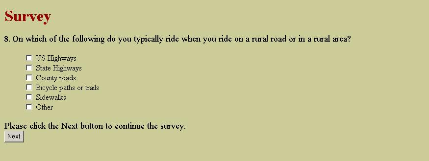
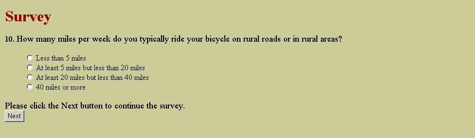
146 138

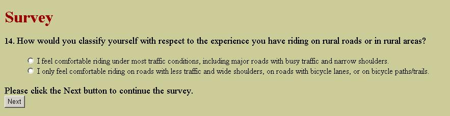
147 139

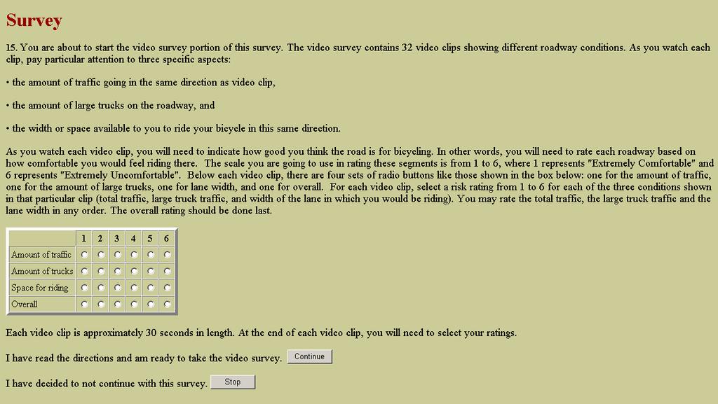
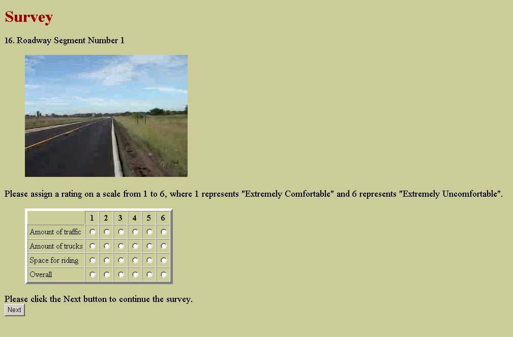
148 140

149 141

150 142

151 143

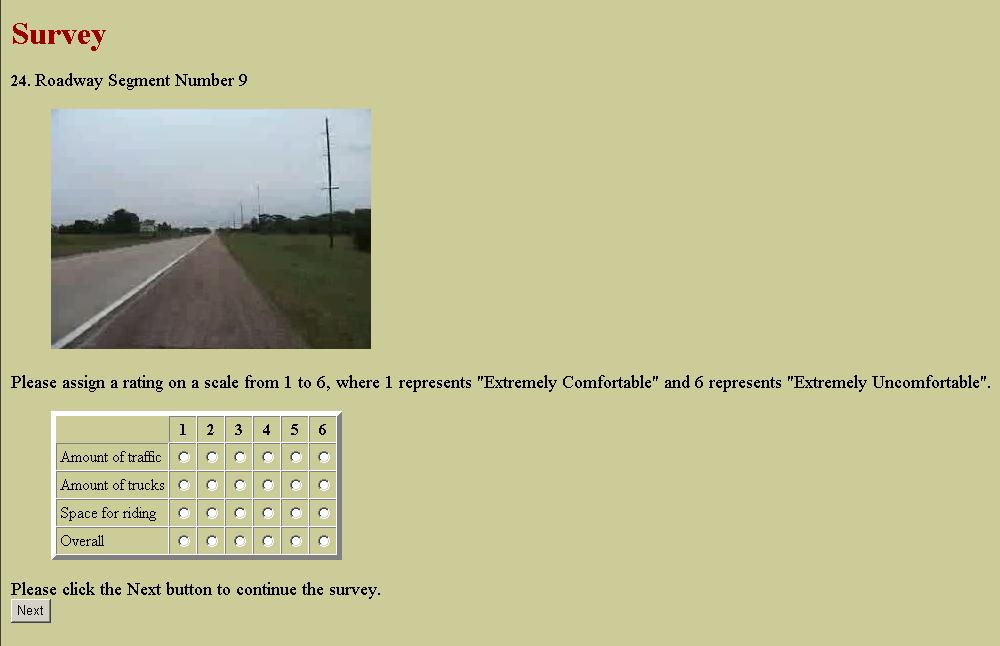
152 144

153 145

154 146

155 147

156 148

157 149

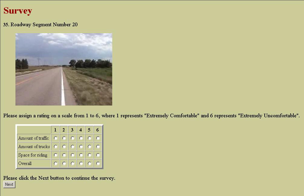
158 150