SPORT-FISHING USE AND VALUE: LOWER SNAKE RIVER RESERVOIRS

Transcription

1 SPORT-FISHING USE AND VALUE: LOWER SNAKE RIVER RESERVOIRS John R. McKean Agricultural Enterprises, Inc. R. G. Taylor University of Idaho Department of Agricultural Economics and Rural Sociology Moscow, Idaho Idaho Experiment Station Bulletin -2 University of Idaho Moscow, Idaho

2 TABLE OF CONTENTS TABLE OF CONTENTS...ii LIST OF FIGURES... LIST OF TABLES... iv iv EXECUTIVE SUMMARY...v SECTION ONE - SPORTFISHING DEMAND...1 Measurement of Economic Value...1 METHODS -- Lower Snake River Reservoir Sport-fishing Demand Survey...4 Reservoir Sportfishing Sites...8 Travel Time Valuation...13 Disequilibrium Labor Market Model...13 Disequilibrium and Equilibrium Labor Market Models...14 Inclusion of Closely Related Goods Prices...15 Travel Cost Demand Variables...16 Prices of a Trip From Home to Site...17 Closely Related Goods Prices...17 Other Exogenous Variables...18 SPORT-FISHING DEMAND RESULTS...18 Demand Elasticities...19 Price Elasticity of Demand...19 Price Elasticity of Closely Related Goods...19 Elasticity With Respect to Other Variables...2 Estimating Consumers Surplus per Trip from Home to Site...21 Model I- Consumers Surplus Per Trip...21 Model II- Consumers Surplus Per Trip...22 Total Annual Consumers Surplus for Sportfishing on the Reservoirs...22 Non-response Adjustment to Total Annual Willingness-To-Pay...22 Other Effects of Separating Single and Multi-destination Trip Price...23 Representation of Reservoirs in the Consumer Surplus Valuation...23 Willingness-to-pay Comparisons...24 The Snake River Reservoirs as an Intervening Opportunity...29 ii

3 Demand and Location...29 Measurement of the Intervening Opportunity Value of the Reservoirs...29 Fish Species Valuation...29 Differences in Trip Value among the Four Reservoirs...38 SECTION TWO - SPORT-FISHING EXPENDITURES Geographic Location of Economic Impacts...41 Angler Spending Distributions...48 Expenditure Per Angler, Per Trip From Home to Site, and per Year...52 Sportfishing Expenditure Rates by Town...53 Angler Lodging...55 Angler Mode of Transportation...55 Importance of Recreation Activities During the Fishing Trip...55 REFERENCES...57 APPENDIX I - Statistical concerns for demand curve estimation APPENDIX II - QUESTIONNAIRES iii

4 LIST OF FIGURES Figure 1 Market demand for fishing...2 Figure 2 Sportfishing demand for an individual...3 Figure 3 Travel Time Versus Fishing Trips per Year...6 Figure 4 Travel cost versus fishing trips per year...7 Figure 5 Map of the Lower Snake River reservoirs...1 Figure 6 Anglers fishing from boat, bank, or both boat and bank...12 Figure 7 Time fishing on site...25 Figure 8 Anglers by distance traveled - fishing demand survey Figure 9 Anglers by distance traveled - spending survey Figure 1 Anglers by amount of purchase from county government...5 Figure 11 Overnight lodging by anglers...54 LIST OF TABLES Table 1 Percent of anglers that typically catch each fish species...9 Table 2 Relative trip values to anglers that typically catch a given fish species type Table 3 Definition of variables...32 Table 4 Model I - Lower Snake River reservoirs...34 Table 5 Model II - Lower Snake River reservoirs: separate prices for single versus multi-destination anglers...35 Table 5-a Effects of exogenous variables on an angler s trips per year...37 Table 6 Average values of variables in the travel cost model by reservoir...39 Table 7-A Expenditures made by anglers traveling to the reservoirs (n= 44) Table 7-B Expenditures made by anglers traveling to the reservoirs (n=411) Table 8-A Expenditures made while staying at the reservoirs (n=44 anglers)...47 Table 8-B Expenditures made while staying at the reservoirs (n= 411 anglers) Table 9-A Expenditures made by anglers returning from the reservoirs (n= 44)...5 Table 9-B Expenditures made by anglers returning from the reservoirs (n=411) Table 1 Type of transportation used by anglers 1/...55 Table 11 Importance of recreation activities during fishing trip...56 iv

5 SPORT-FISHING USE AND VALUE: LOWER SNAKE RIVER RESERVOIRS EXECUTIVE SUMMARY Two surveys were conducted on anglers fishing at the Lower Snake River reservoirs for the purposes of: (1) measuring willingness-to-pay for recreational fishing trips and, (2) measuring expenditures by anglers. The surveys were conducted by a single mailing using a list of names and addresses collected from anglers at the reservoirs during May through October, The sportfishing demand survey resulted in 537 usable responses and the sport-fisher spending survey received 411 usable responses. The response rate for both, rather complex, questionnaires was about 59 percent. The high response rate is thought to be a result of the excellent impression made by the initial on-site contacts, the return address for the questionnaire to the University of Idaho, a two dollar bill included as incentive, and the dedication to fishing by the anglers at the reservoirs. The sportfishing demand analysis used a model that assumed anglers did not (or could not) give up earnings in exchange for more free time for fishing. This model requires extensive data on angler time and money constraints, time and money spent traveling to the reservoir fishing sites, and time and money spent during the fishing trip for a variety of possible activities. The travel cost demand model related fishing trips (from home to site) per year by groups of anglers (average about 2 trips per year) to the dollar costs of the trip, to the time costs of the trip, to the prices on substitute or complementary trip activities, and other independent variables. The dollar cost of the trip was based on reported travel distances from home to site times the average observed (in-sample) cost of $.19/mile for a car divided by the average party size (2.5) yielding 7.6 cents per mile per angler. The statistical demand model also accounted for differences in willingness-to-pay of anglers taking multi-destination trips (4% of the sample) from those with only the reservoirs as their destination. Anglers for whom the reservoirs were an intervening opportunity along their path to a second recreation site had a higher demand for the reservoirs than did those who were not able to include additional non-reservoir sites in their trip. The primary objective of the demand analysis was to estimate willingness-to-pay per trip for fishing at the reservoirs. Consumer surplus (the amount by which total consumer willingness-to-pay exceeds the costs of production) was estimated at $29.23 per person per trip. The average number of fishing trips per year from home to the Lower Snake River reservoirs was resulting in an average annual willingness-to-pay of $592 per year. The total annual willingness-to-pay by anglers was estimated at nearly $2 million dollars per year ($1,956,56) after adjustment of the base value of $1,675,952 for nonresponse bias. The sportfisher spending survey collected detailed information on the types of purchases and the place the purchases occurred. Separate data were collected for the trip to the reservoirs, while onsite at the reservoirs, and on the trip home. Expenditure data for some 26 seller categories were obtained. The data allow measuring the average expenditure by type of purchase for various distances from the reservoirs. The name of the town nearest where each purchase occurred was collected allowing estimation of average purchases for each of the seller categories for a large number of towns. v

6 Average group expenditures were $229 per trip and the group size was 2.5 persons. Angler spending per person per trip was thus nearly $92. Multiplying the per trip cost times the trips per year (2.255) resulted in annual spending of about $1,855 for anglers traveling to the reservoirs. Total annual spending by anglers traveling to the reservoirs is found by multiplying the number of anglers (3,35) times annual spending per angler ($1,855) or 3,35 x $1,855 = $6,13,775 per year. Angler spending that occurred during the Lower Snake River reservoir fishing trips excluded spending made while traveling to other fishing sites and excluded major purchases of boats or other gear, maintenance, storage, insurance and other non-trip related fishing costs. Angler trip expenditures includes non-fishing related purchases made during the trip. The sportfishing demand and spending surveys provided detailed information on samples of individuals who participated in sportfishing on the four Lower Snake River reservoirs. The information provided by these samples was used to infer the spending behavior of anglers on the Lower Snake River reservoirs. In capsule, the data collected by the demand survey provided information that was used to estimate the willingness-to-pay (marginal benefits) by consumers for various amounts of sportfishing. Estimation of the marginal benefits (demand) function allowed calculation of net economic value per fishing trip. The sportfisher spending survey showed spending patterns useful in estimating the stimulus to jobs and business sales in the region created by anglers attracted to the reservoirs. The total economic effects of sportfishing include both the initial spending stimulus on sales, employment, and personal income and the indirect economic effects as the initial spending effects spread throughout the local economy (For an example, see McKean et al. 1998). This study estimates the initial economic effects which will be used in a separate economic multiplier study that estimates the total economic effects. The surveys also provided information on types of fish caught, total catch, transportation, lodging, and other outdoor recreation activities enjoyed by sport-fishers while at the reservoirs. The survey data were used to infer the effect of fishing success rates on frequency of visitation and thus show the recreation value of fish stocks or other factors (such as draw downs) that affect fishing success rate. Research was funded by; Department of the Army, Corps of Engineers, Walla Walla District21 North Third Avenue, Walla Walla, Washington 99362Contract No. DACW D-3. vi

7 SECTION ONE - SPORTFISHING DEMAND Measurement of Economic Value A public enterprise like the Lower Snake River reservoirs differs in two significant ways from a competitive firm. First, the public project is very large relative to the market that it serves; this is one of the reasons that a public agency is involved. Because of the size of the project, as output (fishing access) is restricted the price that people are willing to pay will increase (a movement up the market demand curve). Price is no longer at a fixed level as faced by a small competitive firm. Second, the seller (a public agency) does not act like a private firm which charges a profit-maximizing price. A public project has no equilibrium market price that can easily be observed to indicate value or, i.e., marginal benefit. If output for sportfishing at the reservoirs was supplied by many competitive firms, market equilibrium would occur where the declining market demand curve intersected the rising market supply curve. The competitive market equilibrium is economically efficient because total consumer benefits are maximized where marginal cost equals marginal benefits. If marginal costs exceed marginal benefits in a given market rational consumers will divert their spending to other markets. A competitive market price would indicate the marginal benefit to consumers of an added unit of sportfishing recreation. However, calculation of total economic value produced would require knowledge of the market demand because many consumers would be willing-to-pay more than the equilibrium price. The amount by which total consumer willingness-to-pay exceeds the costs of production is the total net benefit or consumers surplus. If output was supplied by many competitive firms, statistical estimation of a market demand curve could use observed market quantities and prices over time. Economic value (consumers surplus) of a particular output (sportfishing) of a public project also can be found by estimating the consumer demand curve for that output. The economic value of sportfishing on the four reservoirs can be determined if a statistical demand function showing consumer willingness-to-pay for various amounts of sportfishing is estimated. Because market prices cannot be observed, (sportfishing is a non-market good), a surrogate price must be used to model consumer behavior toward sportfishing (U.S. Army Corps of Engineers 1995; Herfindahl and Kneese 1974; McKean and Walsh 1986; Peterson et al. 1992). The sportfishing demand survey collected information on individuals at the reservoirs showing their number of reservoir sportfishing trips per year and their cost of traveling to the reservoirs. The price faced by anglers is the cost of access to the reservoirs (mainly the time and money costs of travel from home to site), and the quantity demanded per year is the number of fishing trips they make to the reservoirs. A demand relationship will show that fewer trips to the reservoirs are made by people who face a larger travel cost to reach the reservoirs from their homes (Clawson and Knetsch 1966). The Travel cost method (TCM) has been preferred by most economists, as it is based on observed market behavior of a cross-section of users in response to direct out-of-pocket and time cost of travel. 1

8 (Loomis 1997) 1 The basic premise of the travel cost method (TCM) is that per capita use of a recreation site will decrease if the out-of-pocket and time costs of traveling from place of origin to the site increase, other things remaining equal. (Water Resources Council 1983, Appendix 1 to Section VIII). Figure 1 shows a market for sportfishing. (It is a convention to show price on the vertical axis and quantity demanded on the horizontal axis). A market supply and demand graph for fishing shows the economic factors affecting all anglers in a region. The demand by anglers for fishing trips is negatively sloped, showing that if the money cost of a trip rises anglers will take fewer trips per year. Examples of how money trip costs Price (Travel cost of a Visit) Market Demand for Fishing Demand Quantity Demanded (Visits per Year) Figure 1 Market demand for fishing Supply might rise include: increased automobile fuel prices, fishing regulators close nearby sites requiring longer trips to reach other sites, entrance fees are increased, boat launching fees are raised, or nearby sites become congested requiring longer trips to obtain the same quality fishing. The supply of fishing opportunities is upward sloping. The upward slope of fishing supply is caused by the need to travel ever further from home to obtain quality fishing if more people enter the regional sportfishing market. Increased fishing-trips in the region can occur when a larger percentage of the population becomes interested in fishing, when more non-local anglers travel to the region to obtain quality fishing, or if the local population expands over time. The market demand/supply graph is useful for describing the aggregate economic relationships affecting angler behavior but a site-demand model is used to place a value on a specific fishing site (such as the Lower Snake River reservoirs.) Figure 2 describes the demand by a typical angler for fishing at the Snake River reservoirs. Angler demand is negatively sloped indicating, as before, that a higher cost or price to visit the fishing site will reduce angler visits per year. The supply curve for a given angler to fish at a given site is horizontal because the distance from home to site, which determines the cost of access, is fixed. The supply curve would shift up if auto fuel prices increased but it would still be horizontal because the number of trips from home to site per year would not influence the cost per trip. The vertical distance between the angler s demand for fishing and the horizontal supply (cost) of 1 Travel cost models are incapable of predicting contingent behavior and involve current users. Another set of economic models, contingent behavior and contingent value models, are typically used for projecting behavior or measuring non-use demand. 2

9 Snake River Sport Fishing Demand: Angler #1 Price (Travel cost of a Visit) Cost to Drive to the River for Angler #1 Equilibrium Area in Triangle is Total Consumer Surplus For Angler #1 Quantity Demanded (Visits per Year) Figure 2 Sportfishing demand for an individual a fishing trip is the net benefit or consumer surplus obtained from a fishing trip. The demand curve shows what the angler would be willing-to-pay for various amounts of fishing trips and the horizontal line is their actual cost of a trip. As more fishing trips per year are taken, the benefits per trip decline until the marginal benefit (added satisfaction to the consumer) from an additional trip equals its cost where cost and demand intersect. The angler does not make any more visits to the reservoirs because the money value to this angler of the added satisfaction from another fishing trip is less than the trip cost. The equilibrium number of visits per year chosen by the angler is at the intersection of the demand curve and the horizontal travel cost line. Each angler has a unique demand curve reflecting how much satisfaction they gain from fishing at the reservoirs, their free time available for fishing, the distance to alternate comparable fishing sites, and other factors that determine their likes and dislikes. Each angler also has a unique horizontal supply curve; at a level determined by the distance from their home to the reservoir fishing site of their choice, the fuel efficiency of their vehicle, reservoir access fees (if any), etc. The critical exogenous variable in the travel cost model is the cost of travel from home to the fishing site. Each angler has a different travel cost (price) for a fishing trip from home to the reservoirs. Variation among anglers in travel cost from home to fishing site (i.e., price variation) creates the Lower Snake River reservoirs site-demand data shown in Figure 3. The statistical demand curve is fitted to the data in Figure 3 using regression analysis. 2 Non monetary factors, such as available free time and relative enjoyment for fishing, will also affect the number of reservoir visits per year. The statistical demand curve should incorporate all the factors which affect the publics willingness-to-pay for sportfishing at the reservoirs. It is the task of the Lower Snake River reservoirs angler survey to include questions that elicit information about anglers that explains their unique willingness-to-pay for sportfishing. The goal of the travel cost demand analysis is to empirically measure the triangular area in Figure 2 which is the net dollar value of satisfaction received or angler willingness-to-pay in excess of the costs of the fishing trips. The triangular area is summed for the 537 anglers in our sample and divided by their average number of trips per year (which, for anglers in our sample was trips 2 It is possible that some anglers might select a residence location close to the reservoirs to minimize cost of travel (Parsons 1991). The travel cost model assumes that this doesn t happen. If anglers locate their residence to minimize distance to the reservoir fishing site then the assumption that travel cost is exogenous is invalid and a simultaneous equation estimation technique would be required. 3

10 per year). This is the estimated consumer surplus per fishing trip or, i.e., net economic value per trip. The estimated average net economic value per trip (consumer surplus per trip), derived from the travel cost model, can be multiplied times the total angler trips from home to the reservoirs in a year to find annual net benefits of the Lower Snake River reservoirs for sportfishing. Figure 3 shows the sample data relating fishing trips per year to the hours required to travel between home and the reservoir fishing site. 3 Figure 4 shows unadjusted sample data relating fishing trips from home to site per year and dollars of travel expense per trip at the reservoirs for 537 respondents. The data shown in both graphs reveal an inverse relationship between money or time required for a fishing trip to the reservoirs and trips demanded per year. Both out-of-pocket cost per trip and hours per trip act as prices for a fishing trip. Even before adjustment for differences among anglers available free time, fishing experience, and other factors affecting angler behavior, it is clearly shown by Figures 3 and 4 that anglers with high travel costs or high travel time per trip take fewer fishing trips per year. Therefore, observations across the sample of 537 anglers can reveal a sportfishing demand relationship. In summary, each price level along a down-sloping demand curve shows the marginal benefit or angler willingness-to-pay for that corresponding output level (number of fishing trips consumed). The gross economic value (total willingness-to-pay) of the sportfishing output of a public project is shown by the area under the statistical demand function. The annual net economic value (consumers surplus) of sportfishing is found by subtracting the sum of the participants access (travel) costs from the sum of their benefit estimates. This is equivalent to summing the consumer surplus triangles for all anglers at the reservoirs. Because the statistical demand function is only for a sample of sport-fishers, the estimated value from the sample must be adjusted upward to reflect total public sportfishing participation at the reservoirs. Estimation of total visitation is beyond the scope of this study and is discussed in other studies. METHODS -- Lower Snake River Reservoir Sport-fishing Demand Survey The Lower Snake River expanded demand survey includes detailed socio-economic information about anglers and data on money and physical time costs of travel, fishing, and other activities both on and off the reservoir fishing sites. The questionnaire used for the mail survey is shown in Appendix II. The questionnaire used in this study is similar to ones that we used previously to study sportfishing demand on the Cache la Poudre River in northern Colorado and for Blue Mesa Reservoir in southern Colorado (Johnson 1989; McKean et al. 1995; McKean et al. 1996). Both of those earlier surveys were by personal interview and used a much smaller sample size. 4 3 Observations over 9 trips year, 9 dollars or 9 hours are not shown because of space limitations. 4 The personal interview surveys had sample sizes of 2 and 15 while the present survey had 537 useable responses. Sample size has varied widely in published water-based recreation studies. Ward (1989) used a sample of 6 mail surveys to estimate multi-site demand for water recreation on four reservoirs in New Mexico; Whitehead ( ) used a personal interview sample of 47 boat anglers for his fishing demand study on the Tar-Pamlico River 4

11 Anglers in this study were contacted at the reservoirs over the period from May through October 1997 and requested to take part in the sportfishing demand mail survey. Most persons contacted on-site were agreeable to receiving a mail questionnaire and provided their name and mailing address. A small share of those contacted preferred a telephone in North Carolina; Laymen, et al. (1996) used a sample of 343 mail surveys to estimate angler demand for chinook salmon in Alaska. 5

12

13

14 interview and provided a telephone number. Our sportfishing demand mail survey resulted in a sample of 537 useable responses out of 576 surveys returned. Some surveys had to be discarded because they were incomplete. A total of 91 surveys were mailed out yielding a useable response rate of 59 percent for the demand model. All 576 surveys were useable for other data, such as the distance from home to the Lower Snake River reservoir fishing site. Reservoir Sportfishing Sites A map of the reservoir region is shown in Figure 5. The Ice Harbor Reservoir and Lower Granite Reservoir fishing sites are relatively close to major population areas, Tri-Cities and Lewiston/Clarkston respectively. Lower Monumental and Little Goose reservoirs are more distant from major population centers. The reservoirs have few opportunities for major on-site purchases. The reservoirs provide high quality fishing - catch rates averaged 7.32 fish per day. The average angler fished 6.56 hours per day. Lower Granite Reservoir is about 39.3 miles in length and has a surface area of 8,9 acres. The upper terminus of the reservoir is Lewiston, Idaho and Clarkston, Washington. The reservoir (Lower Granite Lake) is managed to maintain a water surface at the dam between elevations 724 and 738 in order to maintain a normal operating range between elevations 733 and 738 feet in Lewiston. Backwater levees have been constructed around Lewiston, Idaho. Public boat launching facilities are available at 12 locations. There are 5,777.6 acres of project lands surrounding the reservoir. Little Goose Dam is down river from Lower Granite Dam. The reservoir (Lake Bryan) is about 37.2 miles in length and has a surface area of 1,25 acres. The reservoir is at an elevation of 638 feet. The normal operating pool varies between 633 and 638 feet of elevation. Public boat launching facilities are available at six locations. There are 5,398 acres of project lands surrounding the reservoir. Lower Monumental Dam is down river from Little Goose Dam. The reservoir (Lake Herbert G. West) is 28.1 miles in length and has a surface area of 6,59 acres. The reservoir is at an elevation of 54 feet. The normal operating pool varies between 537 and 54 feet elevation. Public boat launching facilities are available at five locations. There are 8,335.5 acres of project lands surrounding the reservoir. Ice Harbor Dam is down river from Lower Monumental Dam and lies upriver from the confluence of the Snake and Columbia Rivers and the towns of Kennewick, Pasco and Richland. The reservoir (Lake Sacajawea) is 32 miles long and has a surface area of 9,2 acres. The reservoir is at an elevation of 44 feet. The normal operating pool varies between 437 and 44 feet elevation. Public boat launching facilities are available at six locations. There are 3,576 acres of project lands surrounding the reservoir (U.S. Army Corps of Engineers, Internet). 8

15 Table 1 Percent of anglers that typically catch each fish species (537 Observations) Fish Species Percent of Anglers Smallmouth Bass Steelhead Channel Catfish Rainbow Trout Northern Squawfish 32.3 Yellow Perch White Crappie Bluegill Black Crappie 16.2 Largemouth Bass White Sturgeon Pumpkinseed

16 Figure 5 Map of the Lower Snake River reservoirs 1

17 Anglers can expect to catch a large variety of fish in the Lower Snake River reservoirs. The sportfishing demand survey listed twelve fish species that anglers might "typically catch" and anglers were requested to select all that apply. Nearly two-thirds of the sample of anglers selected smallmouth bass as the fish they typically catch. Some of the other most important fishes included steelhead (55 percent), channel catfish (52 percent), and rainbow trout (36 percent). The percentage of the sample of anglers fishing for each species is shown in Table 1. A combination of boat and shoreline were used for fishing by 57 percent of the anglers in our fishing demand sample. About 43 percent of the sample did not have boats for fishing and fished only from the bank (see Figure 6). The typical angler had fished at the Lower Snake River reservoirs for years. Anglers spent an average of 26 days per year fishing at the reservoir site where surveyed and 26.5 days per year fishing at places other than that particular reservoir. The average distance from the fishing site where contacted to the best alternate fishing site was only four miles. Travel Time Valuation There has been disagreement among practitioners in the design of the travel cost model, thus wide variations in estimated values have occurred (Parsons 1991). Researchers have come to realize that nonmarket values measured by the traditional travel cost model are flawed. In most applications, the opportunity time cost of travel has been assumed to be a proportion of money income based on the equilibrium labor market assumption. Disagreements among practitioners have existed on the correct income proportion and thus wide variations in estimated values have occurred. The conventional travel cost models assume labor market equilibrium (Becker 1965) so that the opportunity cost of time used in travel is given by the wage rate (see a following section). However, much dissatisfaction has been expressed over measurement and modeling of opportunity time values. McConnell and Strand (1981) conclude, "The opportunity cost of time is determined by an exceedingly complex array of institutional, social, and economic relationships, and yet its value is crucial in the choice of the types and quantities of recreational experiences." The opportunity time value methodology has been criticized and modified by Bishop and Heberlein (1979), Wilman (198), McConnell and Strand (1981), Ward (1983, 1984), Johnson (1983), Wilman and Pauls (1987), Bockstael et al. (1987), Walsh et al., (1989), Walsh et al. (199), Shaw (1992), Larson (1993), and McKean et al. (1995, 1996). The consensus is that the opportunity time cost component of travel Figure 6 Fishing from boat, bank, or both boat and bank (sample=564) 11 cost has been its weakest part, both empirically and theoretically. Site values

18 may vary fourfold, depending on the value of time. (Fletcher et al. 199).... the cost of travel time remains an empirical mystery. (Randall 1994). Disequilibrium in labor markets may render wage rates irrelevant as a measure of opportunity time cost for many recreationists. For example, Bockstael et al. (1987) found a money/time tradeoff of $6/hour for individuals with fixed work hours and only $17/hour with flexible work hours. The results from our previous studies and this study on the Lower Snake River suggest using a model specifically designed to help overcome disagreements and criticisms of the opportunity time value component of travel cost. We use a model that eliminates the difficult-to-measure marginal value of income from the time cost value. Instead of attempting to estimate a money value of time for each individual in the sample we simply enter the actual time required for travel to the recreation site as first suggested by Brown and Nawas (1973), and Gum and Martin (1975) and applied by Ward (1983,1989). The annual income variable is retained as an income constraint. 5 Disequilibrium Labor Market Model The travel cost model used in this statistical analysis assumes that site visits are priced by both (1) out-of-pocket travel expenses, and (2) opportunity time costs of travel to and from the site. Opportunity time cost has been conventionally defined in economic models as money income foregone (Becker 1965; Water Resources Council 1983). However, a person s consideration of their limited time resources may outweigh money income foregone given labor market disequilibrium and institutional considerations. Persons who actually could substitute time for money income at the margin represent a small part of the population, especially the population of recreationists. Retirees, students, and unemployed persons do not exchange time for income at the margin. Many workers are not allowed by their employment contracts to make this exchange. Weekends and paid vacations of prescribed length are often the norm. Thus, the equilibrium labor market model may apply to certain selfemployed persons, e.g., dentists or high level sales occupations, where individuals, (1) have discretionary work schedules and, (2) can expect that their earnings will decline in proportion to the time spent recreating. (Many professionals can take time off without foregoing any income). The equilibrium labor market subgroup of the population is very small. According to U.S. Bureau of Labor Statistics and National Election Studies (U.S. Bureau of the Census 1993), only 5.4 percent of voting age persons in the U.S. were classified as self-employed in the United States in The labor market equilibrium model applies to less than 5.4 percent of recreationists who are over-represented by retirees and students. Bockstael et al. (1987), hereafter (B-S-H), provide an alternate model in which time and income are not substituted at the margin. B-S-H show that the time and money constraints cannot be collapsed into one when individuals cannot marginally substitute work time for leisure. Thus, money cost and physical travel time per trip from home to site enter as separate price variables in the demand function and discretionary time and income enter as separate constraint variables. Money cost and physical time per trip also enter as separate price variables for closely related time-consuming goods 5 An added advantage of not using income to measure opportunity time value is that colinearity between the time value component of travel cost and the income constraint should be greatly reduced. 12

19 such as alternate fishing sites. The B-S-H travel cost model can be estimated as; r = β + β c + β t + β c + β t + β INC + β DT a 4 a 5 6 (1) where the subscripts o and a refer to own site prices and alternate site prices respectively, c is out-ofpocket travel cost per trip, t is physical travel time per trip, INC is money income, and DT is available discretionary time. Disequilibrium and Equilibrium Labor Market Models The equilibrium labor market model makes the explicit assumption that opportunity time value rises directly with income. Thus, the methodology that we have rejected assumes perfect substitution between work and leisure. McConnell and Strand (1981, 1983) (M-S) specify price in their travel cost demand model as the argument in the right hand side of equation two: r = f [ c + ( t) g ( w) ] (2) where, as before, r is trips from home to site per year, c is out-of-pocket costs per trip, and t is travel time per trip. The term g'(w) is the marginal income foregone per unit time. It is assumed in the M-S model that any increase of travel cost, whether it is out-of-pocket spending or the money value of travel time expended, has an equal marginal effect on visits per year. The term [c + (t)g'(w)] imposed this restriction because it forces the partial effect of a change in out-of-pocket cost (Mf/Mc) to be equal in magnitude to a change in the opportunity time cost Mf/M[(t)g'(w)]. An important distinction in model specification is demonstrated by M-S. The equilibrium labor market model requires that out-of-pocket and opportunity time value costs be added together to force an identical coefficient on both costs. 6 In contrast, the B-S-H disequilibrium labor market model requires separate coefficients to be estimated for out-of-pocket costs and opportunity time value costs. Measurement and statistical problems often beset the full price variable in empirical applications. Even for those self-employed persons who are in labor market equilibrium, measuring marginal income is difficult. Simple income questions are unlikely to elicit true marginal opportunity time cost. Only after-tax earned income should be used when measuring opportunity time cost. Thus, opportunity cost may be overstated for the wealthy whose income may require little of their time. Conversely, students who are investing in education and have little market income will have their true opportunity time costs understated. In practice, marginal income specified by theory is usually replaced with a more easily observable measure consisting of average family income per unit time. Unfortunately, marginal and average values of income are unlikely to be the same. 6 Although the equilibrium labor market model requires that the marginal effects of out-of-pocket cost and income foregone on quantity demanded be equal, empirical results often fail to support the model if the two components of price are entered separately in a regression. 13

20 Inclusion of Closely Related Goods Prices Ward (1983,1984) proposed that the "correct" measure of price in the travel cost model is the minimum expenditure required to travel from home to recreation site and return since any excess of that amount is a purchase of other goods and is not a relevant part of the price of a trip to the site. This own-price definition suggests that the other (excess) spending during the trip is associated with some of the closely related goods whose prices are likely to be important in the demand specification. For example, time-on-site can be an important good and it is often ignored in the specification of the TCM. Yet time-on-site must be a closely related good since the weak complementarity principle upon which measurement of benefits from the TCM is founded implies that time-on-site is essential. Weak complementary was the term used to connect enjoyment of a recreation site to the travel cost to reach it (Maler 1974). It is assumed that a travel cost must be paid in order to enjoy time spent at the recreation site. Without travelling to the site, the site has no recreation value to the consumer and without the ability to spend time at the site the consumer has no reason to pay for the travel. With these assumptions, the cost of travel from home to site can be used as the price associated with a particular recreation site (Loomis et al. 1986). The sign of the coefficient relating trips demanded to particular time "expenditures" associated with the trip is an empirical question. For example, time-on-site or time used for other activities on the trip have prices which include both the opportunity time cost of the individual and a charge against the fixed discretionary time budget. Spending more time-on-site could increase the value of the trip leading to increased trips, but time-on-site could also be substituted for trips. Spending during a trip for goods, both on and off the site, consist of closely related goods which are expected to be complements for trips to the site. Finally, spending for extra travel, either for its own sake, or to visit other sites, can be a substitute or a complement to the site consumption. For example, persons might visit site "a" more often if site "b" could also be visited with a relatively small added time and/or money cost. If the price of "b" rises, then visits to "a" might decrease since the trip to "a" now excludes "b". Conversely, persons might travel more often to "a" since it is now relatively less expensive compared to attaining "b" (McKean et al. 1996). Many recreational trips combine sightseeing and the use of various capital and service items with both travel and the site visit, and include side trips (Walsh et al. 199). Recreation trips are seldom single-purpose and travel is sometimes pleasurable and sometimes not. The effect of these "other activities" on the trip-travel cost relationship can be statistically adjusted for through the inclusion of the relevant prices paid during travel or on-site and for side trips. Furthermore, both trips and onsite recreation are required to exist simultaneously to generate satisfaction or the weak complementarity conditions would be violated (McConnell 1992). A relation between trips and site experiences is indicated such that marginal satisfaction of a trip depends on the corresponding site experiences. Therefore, the demand relationship should contain site quality variables, time-on-site, and goods used on-site, as well as other site conditions. Exclusion of these variables would violate the specification required for the weak complementarity condition which allows use of the TCM to measure benefits. In this study of the Lower Snake River reservoirs, an expanded TCM survey was designed to include money and time costs of on-site time (McConnell 1992), on-site purchases, and the money and time cost of other activities on the trip. These vacation-enhancing closely related goods prices are added to the specification of the conventional TCM demand model. Empirical estimates of partial 14

21 equilibrium demand could suffer underspecification bias if the prices of closely related goods were omitted. 7 Traditional TCM demand models seemingly ignore this well known rule of econometrics and exclude the prices of on-site time, purchases, and other trip activities which are likely to be the principal closely related goods consumed by recreationists. Travel Cost Demand Variables The definitions for the variables in the disequilibrium and equilibrium travel cost models are shown in Table 3. The dependent variable for the travel cost model is (r), annual reported trips from home to the fishing site. Annual fishing trips from home to the four lower Snake River reservoirs is the quantity demanded. Prices of a Trip From Home to Site The money price variable in the B-S-H model is c r, which is the out-of-pocket travel costs to the fishing site. Our mail survey obtained travel costs for most of those surveyed. The average out-ofpocket travel cost was about 19 cents per mile per car. The average party size was 2.5 resulting in a 7.6 cents per mile per angler travel cost. Reported one-way travel distance for each party was multiplied times two and times $.76 to obtain money cost of travel per person per trip. Cost per mile was based on average angler-perceived cost rather than costs constructed from Department of Transportation or American Automobile Association data. Anglers perceived price is the relevant variable when they decide how many fishing trips to take (Donnelly et al. 1985). The physical time price for each individual in the B-S-H model (disequilibrium labor market) is measured by t o which is round trip driving time in hours. Possible differences in sensitivity to time price were accommodated in the model by creating separate time price variables for different occupations. It would be expected that jobs with the least flexibility to interchange work and leisure hours would be the most sensitive to time price. Seven occupation or employment status categories including student, retired and unemployed were obtained in our survey. Dummy variables ( or 1) were created for each of the occupations and the time price, t o, was multiplied times the dummies to create separate price variables for each occupation category. For example, t o3 is either the "self-employed persons" round trip travel time to the fishing site or zero if the angler is not self-employed. In this manner, the price elasticity of demand with respect to travel time c is allowed to vary, or be zero, for each of the 7 Bias in the consumer surplus estimate, created by exclusion of important closely related goods prices, depends on the sign of the coefficient on the excluded variable, and the distribution of trip distances (McKean and Revier 199). Exclusion of the price of a closely related good will bias the estimate of both the intercept and the demand slope estimate (Kmenta 1971). Both these effects bias consumer surplus. Since the expression for consumer surplus generally is nonlinear, the expected consumer surplus is not properly measured by simply taking the area under the demand curve. The distribution of trips along the demand function can affect the bias in consumers surplus, depending on the combination of intercept and slope bias created by the under-specification of the travel cost demand. Both intercept and slope biases and the trip distribution must be known in order to predict the effect of exclusion of the price of a related good on the consumer surplus estimate. 15

22 occupation classes. 8 Closely Related Goods Prices The B-S-H model calls for the inclusion of t a, round trip driving time from home to an alternate fishing site, as the physical time price of an alternate fishing site. This variable was not significant and appeared to be highly correlated with the monetary cost of travel. The remaining alternate site price variable is c a, which is the out-of-pocket travel costs to the most preferred alternate fishing site. This substitute price variable was significant and had the theoretically expected positive sign. (If the angler s best substitute fishing site is costly to reach, more visits to the Lower Snake River reservoirs are likely.) The variable to measure available free time is DT. The discretionary time constraint variable is required for persons in a disequilibrium labor market who cannot substitute time for income at the margin. Restrictions on free time are likely to reduce the number of fishing trips taken. The discretionary time variable has been positive and highly significant in previous disequilibrium labor market recreation demand studies and was highly significant in this study (Bockstael et al. 1987; McKean et al. 1995, 1996). The income constraint variable (INC) is defined as average annual family income resulting from wage earnings. The relation of quantity demanded to income indicates differences in tastes among income groups. Although restrictions on income should reduce overall purchases, it may also cause a shift to inferior types of consumer goods. Thus, the sign on the income coefficient conceptually can be either positive or negative. Two other closely related goods prices were significant in the model: time spent on site at the four reservoirs, t os, and time spent on-site at alternate fishing sites away from the reservoirs during the reservoir fishing trip, t as. The signs of the coefficients for the time variables indicate how they are considered by anglers. As discussed earlier, spending more time-on-site at the reservoirs, (or at alternate sites during the trip), could increase the value of the trip leading to increased trips, but timeon-site could also be substituted for trips. A price variable, c md, measuring money travel cost for the second leg of the trip for anglers visiting a second site away from the Snake River reservoirs was also included. This variable would indicate if the number of trips to the Snake River reservoirs was influenced by the cost of going from the reservoirs to the second site for those with multi-destination trips. Other Exogenous Variables The expected fishing success rate variable, E(Catch) is the individual s previous average catch per day at the Lower Snake River reservoirs. Trips from home to site per year are hypothesized to relate positively to expected fishing success based on the individuals past experience at the reservoirs. The strength of an angler s preferences for fishing over other activities should positively influence the number of fishing trips taken per year. The variable, TASTE = hours fished per day, is used as one 8 Price elasticity with respect to travel time is defined as the percentage reduction in quantity demanded (trips per year) for a one percent increase in time required to travel from home to the fishing site. 16

23 indicator for angler tastes and preferences. A second indicator of taste related particularly to the study site is the number of years that the angler has fished at the reservoirs. The variable FEXP measures this second aspect of taste. Each reservoir may have a unique demand depending on its geographic location and fishing attributes. Each reservoir was represented by a dummy variable in the model. Only Lower Granite Reservoir near the towns of Lewiston and Clarkston showed a significant positive increase in fishing demand relative to the other reservoirs. Age has often been found to influence the demand for various types of outdoor recreation activity. A quadratic function for age was used to allow fishing activity to first rise and then decline with age. A dummy variable (BANK) that identified anglers that fished only from the shoreline versus anglers that used both the reservoir bank and boats for fishing was included in the model. SPORT-FISHING DEMAND RESULTS The t-ratios for all important variables to estimate the value of sportfishing are statistically significant from zero at the 5 percent level of significance or better. Some of the tests for overdispersion, (Cameron and Trivedi 199; Greene 1992), were positive. Therefore, as discussed earlier, the truncated Poisson regression was replaced by the truncated negative binomial regression method. Use of the truncated negative binomial model eliminated the overstatement of the t-ratios found in the Poisson regression results. Demand Elasticities The estimated regression coefficients and elasticities from the truncated negative binomial regression estimation for the Lower Snake River reservoirs sportfishing demand models are reported in Tables 4, 5, and 5-a. Some of the exogenous variables in the truncated negative binomial regressions were log transforms. When the independent variables are log transforms the estimated slope coefficients directly reveal the elasticities. When the independent variables are linear the elasticities are found by multiplying the coefficient times the mean of the independent variable. Elasticity with respect to dummy variables could be estimated for at least three situations, the dummy variable is zero, the dummy variable is one, or the average value of the dummy variable. Given a log transform of the dependent variable, elasticity for a dummy variable is zero if the dummy is zero, the estimated slope coefficient if the dummy is one, and the slope coefficient times the E(dummy) if the average value of the dummy is used. We will report the elasticity for the case where the dummy is one. 9 9 Let the regression equation be ln(r) = " 1 + " 2 D + " 3 ln(z) where Z represents all the continuous independent variables. The equation can be written as r = e ("1 + "2D) Z ("3). Elasticity of r with respect to D is defined as, = (% change in r) / (% change in D) = (Mr/MD)(D/r). Mr/MD =" 2 e ("1 + "2D) Z ("3) ; D can be, 1, or E(D); and r is defined above. Elasticity reduces to, = " 2 D. Thus,, becomes zero if D is zero and, takes the value " 2 if D is one. 17

24 Price Elasticity of Demand Price elasticity with respect to out-of-pocket travel cost is As expected for a regionally unique consumer good, the number of trips per year is not very sensitive to the price. A ten percent increase in travel costs would only reduce participation by 2.8 percent. The elasticity with respect to physical travel time for retirees in the sample is If the time required to reach the site increased by ten percent, visits would decrease by 1.4 percent. Elasticity with respect to travel time for the unemployed is not statistically significant, for self-employed is -.18, for hourly wage earners is -.24, and for professionals is Other occupation categories had very few members represented in the sample and did not have significant coefficients. Price elasticity of time on site is not significant. Price Elasticity of Closely Related Goods Price elasticity for time at the alternate fishing site is.8 and positive, indicating the alternate site is a substitute for the reservoirs. A ten percent increase in the time at an alternate fishing site would cause anglers to increase visits to the reservoirs by.8 percent. Price elasticity for the cost of travel to an alternate fishing site is.9 and positive, again indicating the alternate site is a substitute for the reservoirs. A ten percent increase in the cost to reach an alternate fishing site would cause anglers to increase visits to the reservoirs by.9 percent. Inclusion of substitute price variables is very important to prevent overstatement of estimated consumers surplus. Price elasticity with respect to the cost of the second leg of the journey for those visiting more than one site (other than at the Snake River reservoirs) was not statistically significant. Elasticity With Respect to Other Variables Income elasticity is Quantity demanded (fishing trips from home to the reservoirs per year), was negatively related to income. It is not unusual to find that sportfishing near home is an inferior good that appeals more to lower than to high income families. Elasticity with respect to discretionary time is.21. As in past studies, the discretionary time was positive and highly significant. A ten percent increase in free time results in a 2.1 percent increase in fishing trips to the reservoirs. As expected, available free time acts as a powerful constraint on the number of fishing trips taken per year. Elasticity with respect to TASTE was positive showing that anglers who fished more hours per day were likely to take more fishing trips per year. Those who fished ten percent longer per day would tend to take 2.7 percent more fishing trips per year. The elasticity for expected fishing success (past average catch per trip) shows that a ten percent increase in the catch rate results in a 1.4 percent increase in fishing trips to the reservoirs per year. The fishing success variable has policy applications for reservoir fish management. The fishing experience variable showed that those who have fished the reservoirs over a long period of time tend to make more fishing trips to the reservoirs. A ten percent increase in years fished at the reservoirs results in a 2.3 percent increase in annual trips to the reservoirs. The dummy variables to distinguish demand among the reservoirs were mostly insignificant. Only the dummy demand-shift variable for Lower Granite Reservoir (GRAN) was significant. The 18

25 coefficient estimated for the dummy variable indicated that many more fishing trips are demanded by anglers at Lower Granite Reservoir compared to the other reservoirs after accounting for other variables in the model (such as travel distance 1 etc.). For example, if ten percent of the anglers switched from other reservoirs to Lower Granite, average trips per year would rise by 4.7 percent. The model also indicates that anglers at Lower Granite Reservoir take 47 percent more fishing trips than do anglers at the three other reservoirs. This result is consistent with the average trips per year in the demand survey sample. Anglers at Lower Granite Reservoir take trips per year compared with at Little Goose, at Lower Monumental, and at Ice Harbor. Reservoir dummy variables to allow a shift in the slope coefficient on monetary price were also attempted but were all insignificant. Thus, the price elasticity of sportfishing demand and consumers surplus per angler do not differ by reservoir. Sample size is too small to permit estimating the model for anglers surveyed at a single reservoir. Age (A) and age squared (AS) had the expected signs. The quadratic function indicates that trips per year first increases with age and then declines. The dummy variable indicating fished from bank only versus fished from both a boat and the shoreline had a positive coefficient. Those who fished only from the bank would take 16 percent more fishing trips per year than those who used both a boat or the bank for fishing. Thus, those without boats had a slightly greater demand for fishing at the reservoirs than those with a boat. The t-value for this variable is quite low and its confidence interval will include zero at the 5 percent level of significance but it is significantly different from zero at the ten percent level. Estimating Consumers Surplus per Trip from Home to Site Consumers surplus was estimated using the result shown in Hellerstein and Mendelsohn (1993) for consumer utility (satisfaction) maximization subject to an income constraint, and where trips are a nonnegative integer. They show that the conventional formula to find consumer surplus for a semi-log model also holds for the case of the integer constrained quantity demanded variable. The Poisson and negative binomial regressions, with a linear relation on the explanatory own monetary price variable are equivalent to a semi-log functional form. Adamowicz et al. (1989) show that the annual consumers surplus estimate for demand with continuous variables is E(r)/(-ß), where ß is the estimated slope on price and E(r) is average annual visits. Consumers surplus per trip from home to site is 1/(-ß). (Also note that the estimate of consumers surplus is invariant to the distribution of trips along the demand curve when surplus is a linear function of Q. Thus, it is not necessary to numerically calculate surplus for each data point and sum as would be the case if the surplus function was nonlinear.) Model I- Consumers Surplus Per Trip Model I estimated consumers surplus per trip, from home to site, assuming travel cost of $.19/car mile (7.6 cents per mile for 2.5 anglers in party). Estimated coefficients for the travel cost model with labor market disequilibrium, and assuming travel cost per mile of 7.6 cents per mile per 1 Average travel distance for the demand survey sample was 54.4 miles at Lower Granite, 77.3 miles at Little Goose, 53.7 miles at Lower Monumental, and 48. miles at Ice Harbor. 19

26 person are shown in Table 4. Application of truncated negative binomial regression, and using anglerreported travel distance times $.76 per mile per person to estimate out-of-pocket travel costs, results in an estimated coefficient of out-of-pocket travel cost. Consumers surplus per angler per trip is the reciprocal or $ Average angler trips per year in our sample was Total surplus per angler per year is average annual trips x surplus per trip or x $32.23 = $653 per year. The estimated elasticities changed markedly when the Poisson regression was used in place of the negative binomial regression and the estimated consumer surplus decreased greatly, ($14.26 per person per visit versus $31.53 per person per visit for the negative binomial). Annual consumers surplus would only be $289 using the Poisson regression estimate. 2

27 Model II- Consumers Surplus Per Trip Model II estimated consumers surplus per trip from home to site with separate estimates for single and multi-destination anglers assuming travel cost of $.19/car mile (7.6 cents per mile for 2.5 anglers in party) This model, shown in Tables 5 and 5-a, empirically measures the difference in site values for the Snake River reservoirs to single destination and multi-destination anglers. Separate money price variables are entered for anglers taking single and multi-destination trips. As expected, multi-destination anglers place a higher value on the Snake River reservoir site ($39.17 per person per visit) than single destination anglers ($21.31 per person per visit). In contrast, if all anglers are pooled together in the statistical model their value for a visit to the site is estimated at $32.23 (See Table 4). Disaggregation of multi-destination anglers from single destination anglers in the statistical model to find separate site values (see Tables 5 and 5-a) and recombining the values reduced the site value estimate slightly from $32.23 to $29.23 per person visit. The values estimated for multi-destination and single destination anglers are combined using their respective shares in the sample as weights, (.4223 x $4.49) + ( x $21.65) = $29.23 per person per visit. Total surplus per angler per year is average annual trips x surplus per trip or x $29.23 = $592 per year. 11 Total Annual Consumers Surplus for Sportfishing on the Reservoirs An important objective of the demand analysis was to estimate total annual willingness-to-pay for fishing on the four Lower Snake River Reservoirs. As discussed above, consumer surplus was estimated at $29.23 per person per travel cost trip. The average number of sportfishing trips per year from home to the free flowing Snake River was resulting in an average annual willingness-topay of $592 per year per angler. The annual value of the sport-fishery or willingness-to-pay by our sample of 537 anglers is $592 x 537 = $317,94. The total annual willingness-to-pay for all anglers requires knowledge of the total population of anglers which fish on the reservoir. The number of anglers can be calculated from our sample values for hours per day fished and days fished per year combined with the estimated total annual hours fished on the reservoirs (Normandeau Associates et al. 1998a). Hours fished per year for the average angler is estimated from the product of average hours per day (6.56 hours) times average days per year (26.34) or 6.56 x = hours fished per year for an angler. The estimated total annual hours fished on the reservoirs was 489,215. Dividing total annual hours fished by our estimate of hours per year for an individual yields total anglers or 489,215/172.8 = 2,831 unique anglers on the reservoirs. Multiplying annual value per angler times the number of unique anglers yields total annual willingness-to-pay of $592 x 2,831 = $1,675,952. Non-response Adjustment to Total Annual Willingness-To-Pay An adjustment for bias caused by non-response could increase the total annual willingness-topay (and angler expenditures also) by as much as 16.7 percent. About 41 percent of anglers contacted did not return a useable survey. A survey of non-responders was conducted for this data set. A 11 Average annual trips is virtually the same for single destination and multi-destination anglers so a single number (2.255) is used in the weighting. 21

28 telephone survey on non-responding anglers resulted in an average of 13 trips per year compared to about 2 trips per year for those who did respond. These data suggest about 35 percent less participation by non-respondents. A crude adjustment for non-response bias assumes that the 35 percent reduction in trips per year also applies to angler hours per year from our survey. Given that assumption, the average hours per year remains for responders and becomes x (1-.35) for non-responders and the adjusted average hours per angler is [172.8 x.59] + [172.8 x (1-.35) x.41] = 148 where the response rate was.59 and the non-response rate was.41. The result of the adjustment for lower participation by non-responders is to lower the hours per year from to 148 which is a 14.4 percent reduction in estimated average fishing hours per year per angler. As before, the number of unique anglers was estimated by dividing total angler hours fished per year (Normandeau Associates et al. 1998a) by hours per angler (489,215/148 = 3,35) unique anglers. Compared to our previous estimate of 2,831 unique anglers before the adjustment for non-response, this is a 16.7 percent increase in unique anglers. Multiplying annual value per angler times the number of unique anglers yields total annual willingness-to-pay of $592 x 3,35 = $1,956,56 compared to $1,675,952 prior to the adjustment for non-response bias. Other Effects of Separating Single and Multi-destination Trip Price With the exception of the time at alternate site variable, the estimated coefficients in the model are little changed by the separation of single and multi-destination trip prices. The coefficient on the time at alternate site variable is reduced in size and the t-value falls drastically. The estimated coefficient for the time at alternate site variable is no longer significantly different from zero. It is likely that the time on alternate site variable is highly correlated with the money price of multi-destination trips. Multicolinearity among variables in a regression causes the t-values to decline. Representation of Reservoirs in the Consumer Surplus Valuation The sample data are weighted most heavily toward the reservoirs that are close to population centers and receive the most recreation use. The reservoirs listed in order of sample share are: Lower Granite 48.9%, Ice Harbor 25.2%, Little Goose 15.3%, and Lower Monumental 1.6%. The travel cost data set has sample shares that closely match those of the creel survey (aerial counts) that provided our sample name list. The aerial counts showed the following percentages by reservoir: Lower Granite 44.9%, Ice Harbor 25.%, Little Goose 14.1%, and Lower Monumental 16.%. Overall recreation use in the reservoirs is reported in Appendix J (recreation) of the Columbia River System Operation Review (1995). Using a seven year ( ) average of visitor-days results in: Lower Granite 64%, Ice Harbor 2%, Little Goose 1%, and Lower Monumental 6%. Angler visitation as a percent of total recreation visitation at Lower Granite is about half that of the other reservoirs. This is because Lower Granite attracts many hikers from the towns of Lewiston and Clarkston which abut the reservoir. Thus, if adjusted total recreation visitor-days is a guide, our sportfishing demand survey attached the appropriate sampling priority to the four reservoirs. 22

29 Willingness-to-pay Comparisons Comparisons of net benefits for fishing among demand studies is difficult because of differences in the units of measurement of consumption or output. Comparisons of value per person trip are flawed unless all studies compared have similar lengths of stay. Comparisons of value per person per day are difficult because some sites and fish species are fishable all day (or even at night) and others only at certain hours. Conversion problems for sportfishing consumption data makes exact comparison among studies impossible. Anglers at the Snake River reservoirs spent about 19 hours fishing per trip, 4.67 hours on the round trip travel between their home and the reservoirs, and 4.16 hours on other recreation at the reservoirs. However, the time on site distribution is bimodal (see Figure 7). The majority of anglers fish 1-12 hours per trip but a second group fish 48 or more hours per trip. The median time fishing on site is only 7 hours. Conversion of these consumption data into meaningful standard units of comparison, such as recreation-days consumed, is difficult. Many studies are quite old and the purchasing power of the dollar has declined over time. Adjustment of values found in older studies to current purchasing power can be attempted using the consumer price index. Another problem with older studies is the changes in both economic and statistical models used to measure value. Adjustment for different travel cost model methodologies, as well as contingent value methodologies, and inflation, is shown in 23

30

31 Walsh et al. 1988a, 198b and Walsh et al Some of the more recent studies used higher cost per mile than we did for travel and also used income rate as opportunity time cost that was added to the monetary costs of travel. If these outmoded methods resulted in an overstatement of travel cost, a near proportional overstatement of estimated consumer surplus will occur. In addition, some of the studies used Poisson regression and obtained extremely large t-values. Although no test for over-dispersion was mentioned, the very high t-values suggest that the requirement of Poisson regression that the mean and variance of trips per year be equal was violated. If that is the case, the Poisson regressions are inappropriate and should have been replaced with negative binomial regression. A study by Cameron et al. (1996) developed individual travel cost recreation models to predict the effect of water levels on all types of recreation at reservoirs and rivers in the Columbia River Basin. The baseline (1993 water levels) estimates of consumer surplus varied between $13 per person per summer month and $99 per person per summer month over the nine sites. (One of the sites was Lower Granite Reservoir). Annual estimates were not reported in this article. The Cameron et al. (1996) recreation demand study was reported in Appendix J-1 for the Corps Columbia River System Operation Review (CRSOR) (1995). The study included recreation at Lower Granite Reservoir with a sample of about 168 persons. The results for Lower Granite were extrapolated to the other three Lower Snake River reservoirs. Consumer surplus per recreation day for summer recreation can be found using average visitor days shown in (CRSOR) Tables 6,2g-6,2j and total summer consumer surplus shown in Tables 6,3g-6,3j. Division of total consumer surplus by average recreation days result in: Ice Harbor $51.21 per recreation day, Lower Monumental $4.33 per recreation day, Little Goose $42.69 per recreation day, and Lower Granite $35.4 per recreation day. Recreation days varied from 138,4 at Lower Monumental to 1,67,6 at Lower Granite. Values found for other reservoirs in the study included John Day $2.14 per recreation day, Lake Roosevelt $53.27 per recreation day, and Dworshak $54.1 per recreation day. Some of the values found in Cameron et al. (1996) are very high. Changes in consumer surplus estimated by the travel cost method are almost directly proportional to the changes in travel cost value that is used as price in the demand function. One reason for the high values in the CRSOR study is that the vehicle cost used in the price variable was $.29 cents per mile (Department of Transportation estimate) whereas our vehicle cost was $.19 per mile (based on our survey data). The price perceived by travelers is the appropriate measure. DOT data include fixed costs that are not relevant when making incremental trip decisions (Donnelly et al. 1985). In addition, the study added in an opportunity time cost of travel based on estimated travel time valued at the reported average wage rate (see CRSOR, Cameron et al. 1996, Appendix J-1, bottom of Table 5,4). Our methodology did not include a money cost of time in travel cost and physical travel time was included as a separate site price variable. Their assumption that all recreationists give up earnings when traveling to the site is incorrect based on their own survey data. The fraction of persons who stated they gave up some income to visit the sites appears to be abut 1 percent (about 19 persons) in their sample of 186 at Lower Granite Reservoir (see CRSOR, Cameron et al. 1996, Appendix B2 Survey Results part E, About Your 25

32 Typical Trips). 12 The ten percent of visitors that gave up some income, probably did so either on the way to the site or on the return trip but not both ways. The appropriate foregone income amount would only apply to half the trip time and to only ten percent of the visitors. Based on the survey characteristics of typical trips, the foregone income component of travel cost was overstated by about 95 percent. Their travel cost measure also included lodging costs which are discretionary and are not usually considered part of cost of a recreation trip (CRSOR, Appendix C). Their average round trip transportation cost to travel to the Lower Snake River reservoirs was about $23.37 per trip per person whereas ours was about $8.88 per trip per person. The average distance from home to site was only 58 miles in our survey thus the travel cost per trip per person was (116 miles x $.19/mile / 2.5 persons = $8.82). Englin et al. (1997) reported the results of a travel cost demand analysis based on telephone interview of freshwater anglers in New York, New Hampshire, Vermont, Maine, and a sample of lake anglers in the upper northeastern U.S. They found a consumer surplus value of $47 per trip. The number of persons traveling together in a group was not reported. Olsen et al. (1991) use a contingent value survey to obtain estimates for steelhead and salmon fishing in the Columbia River Basin including the lower Columbia River. Their estimate is for $9 per person per trip for steelhead. The average trip length was about two days with.68 steelhead caught on average during the trip. Fishing the lower Columbia River is not directly comparable with the reservoirs because it is primarily steelhead and salmon fishing. McKean et al. (1996) used the travel cost method with data collected by personal interview survey (Johnson 1989) on Blue Mesa Reservoir in south central Colorado. The data were collected in Consumer surplus per trip was estimated to be $69. With an average of 3.66 persons per party the consumer surplus per person per trip was $ Adjusting for inflation between 1986 and 1998 would bring the Blue Mesa Reservoir trip value close to the $28.5 per person per trip as found in this study. However, the average time on site for the Blue Mesa anglers was three days, which is longer than for this study. 13 As noted earlier, the questionnaire, and statistical and economic models developed for the Blue Mesa Reservoir study are nearly the same as in this study. Wade et al. (1988) applied a zonal travel cost model (data are aggregated by distance zones rather that using individual observations on anglers) to study cold water fishing at four large reservoirs in northern California. The 1985 study found a value for reservoir fishing of $18.24 per person per day. Fiore and Ward (1987) used a zonal travel cost model to estimate the value of cold water fishing at Heron Reservoir in New Mexico. The 1981 study found a value for trout fishing of $9.25 per person per day. Fiore and Ward (1987) also studied the value of warm water fishing at Elephant Butte Reservoir in New Mexico. The primary species caught was white bass. Some largemouth bass, catfish, and walleye we also caught. A zonal travel cost model using 1981 data resulted in a value per fishing site. 12 Our survey resulted in 11.9 percent of the sample indicating they gave up some income to travel to the 13 Average fishing time on site per trip from the demand survey sample was 2.7 hours for Lower Granite, 23.6 hours at Little Goose, 15.8 hours at Lower Monumental, and 13.5 hours at Ice Harbor. The average over the four reservoirs was 19.1 hours. 26

33 person day of $ Palm and Malvestuto (1983) used the individual observation travel cost model to estimate the value of warm water fishing at West Point Reservoir in Georgia. The study resulted in a value of $8.9 per person per day. Loomis et al. (1993) used the zonal travel cost method (as opposed to individual observations on anglers used here) to estimate value per angler per day at 26 Corps reservoirs in 198. The reservoirs were in the Little Rock, Nashville, and Sacramento Corps districts. The data were limited to exit surveys of day use visitors which provided the ZIP code of origin (which necessitated the zonal approach). Data for other variables in the fishing demand model were obtained from the Corps and the Census. Consumer surplus value per visit varied from $2.7 (Sacramento) to $12.96 (Nashville). The travel cost consumer surplus values would vary from about $4 to $25 per person per visit after adjusting for inflation between 198 and Oster et al. (1987) studied Flaming Gorge Reservoir in south Wyoming. He used the zonal travel cost method. The 1986 study found a value of $9.78 per person per day. Layman et al. (1996) measured willingness-to-pay for chinook salmon fishing on the Gulkana River in Alaska. They couldn t decide on the best method to value the opportunity cost of time and show consumer surplus for income foregone equal to zero, 3, 6 and 1 percent of the wage rate. They also could not decide whether to use angler-reported travel costs or cost constructed from map distances and cost per mile from the American Automobile Association. The result was eight estimates of consumer surplus ranging from $17 per day to $45.6 per day. Consumer surplus was slightly higher for angler-reported cost than for the constructed costs and much higher when 1 percent of income was used as the opportunity cost of time while traveling. 27

34 The Snake River Reservoirs as an Intervening Opportunity Demand and Location About forty percent of the anglers in our sample chose to visit a second recreation site during their fishing trip. 14 Anglers traveling on to another fishing site spent an average of $22 to go there and stayed an average of 7.6 hours. Anglers traveling on to another site for other types of recreation spent an average of $12.5 to go there and stayed an average of 5.7 hours. The location of the Snake River reservoirs adjacent to other recreation sites increases their visitation and thus their recreation value. Much of the visitation to the Snake River reservoirs is attracted there at least partly because they are enroute to other desired fishing or recreation sites. Reservoirs with the same attributes as the Snake River reservoirs but which were located off the path followed by anglers among sites would have less recreation value. Anglers who visit the Snake River reservoirs as part of a longer trip are expected to place a higher value on their visit (or, i.e., for the same travel cost to visit more often) than anglers who only travel to the reservoir and return home. A higher value is received by the multi-destination anglers because their trip from home to site contains more complementary inputs as discussed in a previous section. Not all anglers can utilize the path among recreation sites either because of time constraints or because of the location of their residence vis a vis the reservoirs. But many (4 percent) do take advantage of the multi-destination opportunity. The fact that the Snake River reservoirs are part of a multi-destination opportunity makes them more valuable to anglers able to utilize the opportunity. If, for some reason, these multi-destination visitors were excluded from the sample the actual visitation and true site value of the reservoirs could be understated. A model which separates the price effects for single and multi-destination anglers is shown in Tables 5 and 5-a. Measurement of the Intervening Opportunity Value of the Reservoirs The intervening opportunity value of the Snake River reservoirs can be found by comparing the value with the existing share of multi-destination trips ($28.49/trip) to the value if only single destination trips occurred. The extra value of the Lower Snake River reservoir fishing site, would be [annual trips] x [$ $21.31]. This location value is for the existing share of anglers that are multidestination (4 percent). If more anglers could take advantage of multidestination trips the locational value of the reservoirs would rise. The intervening opportunity value of the reservoirs would disappear if the other recreation sites were eliminated, thus some economists would exclude the intervening opportunity value from the benefits attributed to the Snake River reservoirs. However, visitation and willingness-to-pay for fishing at the Snake River reservoirs is boosted by their location along the path to other recreation sites, (as shown by the statistical model in Tables 5 and 5-a), and neither this path nor the recreation sites that created it is likely to change greatly over the time period of the planning horizon. 14 None of the multi-destination anglers indicated a second site used for non-recreation activity. 28

35 Fish Species Valuation Estimation of the value (consumers surplus per person per trip) for a specific fish species is problematic since most anglers have the expectation of catching more than one kind of species. Price variables were defined by constructing a dummy variable for each of the species (see Table 1) that anglers were asked about. The fish species ( or 1) dummy variable was multiplied times their price of a trip (out-of-pocket travel cost valued at 7.6 cents per person per mile). Because most anglers expected to catch several kinds of species, some of the species dummy/price interaction variables were highly correlated with one another. A separate demand model regression was run for each species in order to avoid the colinearity. Thus, the estimated values represent the value primarily of the listed fish but may also include value attributed to other fishes on the list. Changes in the availability of one species could affect the value attributed to another. The presence of numerous species in the reservoirs may increase the expected catch rate which would increase the value of fishing in general. Other factors that vary by species, such as time spent fishing during the trip (shown in Table 2) could also contribute to the trip value. Time spent fishing during the trip, and several other fishing demand variables that vary by species are included in the regression model. If the demand model was properly specified, the model should isolate the effect of fish species on value of the trip. 29

36 Table 2 Relative trip values to anglers that typically catch a given fish species type. (Travel cost per mile assumed to be 7.6 cents per person). Fish Species Cases Avg. Fishing Time Per Trip (Hours) t-ratio on price Consumer Surplus Per Person Per Trip From Home to Site Channel Catfish $63.25 Smallmouth Bass $56.72 Northern Squawfish $55.77 Steelhead $5.92 White Crappie $47.65 Bluegill $43.73 Sturgeon $4.18 Rainbow Trout $37. Yellow Perch $33.93 Black Crappie $23.17 Largemouth Bass $22.28 Pumpkinseed (not sig.) $2.41 (not sig.) Table 2 shows both the t-values on the coefficients of the price variable and estimated consumer surplus per trip. The t-values (the value of the estimated coefficient divided by its estimated standard error) indicate the relative reliability of the consumer surplus estimates. Given the closeness in value of the estimated coefficients on price and the size of the standard errors of the coefficients, it is clear that the 95 percent confidence intervals on the coefficients (plus or minus the standard error times 1.96 for a t distribution) overlap. The estimated values provide a ranking of the species for the given species mix available at the reservoirs. Values for fish trips to catch all species of fish studied, except the pumpkinseed species, are significantly greater than zero. 3

37 Table 3 Definition of variables 15 Variable r c o L(t o1 ) L(t o2 ) L(t o3 ) Description annual trips from home to the Lower Snake River reservoir fishing site (dependent variable). the angler s out-of-pocket round trip travel cost to the fishing site, in dollars. "retirees" round trip travel time to the fishing site, in hours. "unemployed persons" round trip travel time to the fishing site, in hours. "self-employed persons" round trip travel time to the fishing site, in hours. L(t o4 ) "hourly wage earners" round trip travel time to the fishing site, in hours. L(t o5 ) "professionals" round trip travel time to the fishing site, in hours. c a L(t as ) the angler s out-of-pocket travel cost to an alternate fishing site away from the reservoirs, in dollars. time spent at an alternative fishing site away from the reservoirs during the trip, in hours. L(t os ) time spent on-site at the reservoirs fishing during the trip, in hours. c md the angler s out-of-pocket travel cost (if any) for the second leg of the trip for anglers visiting a second site away from the Snake River reservoirs. L(INC) annual family earned income, in dollars. L(DT) L(E(Catch)) the angler s discretionary time available per year, in days. the angler s expected catch rate per day at the reservoirs based on past experience. L(Taste) the angler s typical number of hours fished per day. FEXP GRAN A BANK the angler s total fishing experience at the reservoirs, in years. a dummy variable that is one for persons fishing at Lower Granite Reservoir and zero for persons fishing at any of the other reservoirs. the angler s age, in years; and AS = age squared. a dummy variable, one for persons who only fish from the bank and zero for those who either fish from boats or fish both from bank and boat. 15 L in front of the variable indicates a log transformation. 31

38 Table 4 Model I - Lower Snake River reservoirs Variable Coefficient t-ratio Mean of Variable Elasticity Constant na na c r L(t o1 ) L(t o2 ) not significant L(t o3 ) L(t o4 ) L(t o5 ) L(t os ) L(t as ) c a c md not significant L(INC) L(DT) L(Taste) L(E(Catch)) FEXP GRAN A AS BANK Travel cost per mile per angler assumed to be $.76. Truncated Negative Binomial Regression, r = trips per year to the reservoirs (r = dependent variable), mean r = R 2 =.25 (Estimated by a regression of the predicted values of trips from the truncated negative binomial model on the actual values.) 32

39 Table 5 Model II - Lower Snake River reservoirs: separate prices for single versus multi-destination anglers Variable Coefficient t-ratio Mean of Variable Elasticity Constant na na c o single site c o multiple site L(t o1 ) L(t o2 ) not signif L(t o3 ) L(t o4 ) L(t o5 ) L(t os ) L(t as ) not signif c a c md not signif L(INC) L(DT) L(Taste) L(E(Catch)) FEXP GRAN A AS BANK Truncated Negative Binomial Regression 16, r = trips per year from home to the reservoirs (r = dependent variable), mean r = R 2 =.29 (Estimated by a regression of the predicted values of trips from the truncated negative binomial model on the actual values.) 16 See Appendix I for a discussion of the statistical methodology. 33

40 Table 5-a Effects of exogenous variables on an angler s trips per year Exogenous Variable Effect on Trips/Year of a +1% Change Angler s Money Cost of Round Trip (single destination trip) ($/trip) -3.8% Angler s Money Cost of Round Trip (multiple destination trip) ($/trip) -2.5% Retiree Angler s Round Trip Travel Time (hours/trip) -1.3% Unemployed Angler s Round Trip Travel Time (hours/trip) not significant Self-Employed Angler s Round Trip Travel Time (hours/trip) -1.5% Hourly Wage Job Angler s Round Trip Travel Time (hours/trip) -2.3% Professional Job Angler s Round Trip Travel Time (hours/trip) -1.4% Time Spent at the Lower Snake River Reservoirs Fishing (hours/trip) -1.2% Time Spent Fishing at Alternate Site (not at reservoirs) (hours/trip) Angler s Money Cost of Round Trip to Alternate Fishing Site (not at reservoirs) ($/trip) Angler s Money Cost (if any) of the Second Leg of the Journey To Another Recreation Site ($/trip) not significant.8% not significant Annual Family Earned Income ($/year) -2.1% Angler s Discretionary Time (days/year) 2.% Angler s Average Hours per Day Spent Fishing When on Fishing Trips 2.9% Angler s Expected Fish Catch at Lower Snake River Reservoirs 1.4% Angler s Total Years of Fishing Experience 2.2% If Fishing Trip was to Lower Granite Reservoir 4.7% Age - Age Squared - If Angler Fished from Bank Rather than Bank or Boat 1.7% 34

41 Differences in Trip Value among the Four Reservoirs The travel cost price variable was introduced separately for each reservoir in the demand equation. This allowed getting separate estimates of value per angler per trip (from home to reservoir) for each reservoir. The trip value results are as follows: $ Lower Granite Reservoir, $27.66 per person per trip $ Little Goose Reservoir, $54.49 per person per trip $ Lower Monumental Reservoir, $22.69 per person per trip $ Ice Harbor Reservoir, $35.75 per person per trip. Differences among the reservoirs in average values of certain variables may shed some light on the differences in value of a fishing trip among reservoirs found by the travel cost model. In particular, the above normal value of a trip to Little Goose Reservoir requires explanation. Data from the on-site survey indicates that Little Goose Reservoir has far more visitors than the other reservoirs from the north including Pullman, Colfax, and as far away as Spokane. The other major source of visitors is Walla Walla and Tri-Cities. Table 6 shows that anglers traveling to Little Goose Reservoir travel more miles (one way) 8.3 versus miles for the other reservoirs. Travel time round trip is 6.65 hours for Little Goose Reservoir versus for the other reservoirs. Cost of the travel is $58.5 versus $ $28.36 for the other reservoirs. In summary, anglers at Little Goose are willing to travel more miles to get there, and spend more dollars and time to get there. In terms of the travel cost demand model, anglers are willing to pay a higher access price at Little Goose Reservoir than do anglers at the other Lower Snake River reservoirs. 35

42 Table 6 Average values of variables in the travel cost model by reservoir Variable Lower Granite Little Goose Lower Monumental Ice Harbor Hours Per Day Fishing Days Per Year Fish at Reservoirs Days Per Year Fish at Other Places Typical Catch Per Day at Reservoirs Miles From Home to Reservoirs Hours to Travel From Home to Reservoirs and Back Dollar Cost to Travel from Home to Reservoirs and Back ($) Hours of Recreation at Other Places During Trip to Res. Number of Fishing Trips Per Year to Reservoirs Hours Fish at Reservoirs During a Trip Hours Fish at Other Sites Than Reservoirs During Trip Percent Steelhead Anglers 1/ / Steelhead is among the fish anglers typically catch. 36

43 Part of the reason anglers are willing to pay more to fish at Little Goose Reservoir may be because of the direct route and part due to the good marina facilities and camper sites at Little Goose Reservoir. Table 6 shows that anglers at Little Goose Reservoir tend to fish more hours per day at all sites indicating a higher preference for fishing than anglers at the other reservoirs. Thus, Little Goose Reservoir anglers may have a higher demand or willingness to pay for fishing in general. Table 6 shows that anglers at Little Goose Reservoir fish there much longer during a trip, hours versus hours at the other reservoirs. Furthermore, Table 6 shows that Little Goose Reservoir anglers spend hours on non-fishing recreation at places other than the reservoirs during a fishing trip compared to at other reservoirs. In summary, many Little Goose Reservoir anglers must visit other recreation sites during their fishing trip. Little Goose Reservoir anglers spend more per mile of travel. Dividing the cost of a trip ($58.5 by twice the distance from home to site (2 x 8.3) yields a cost per mile of $.36. Cost per mile for anglers traveling to the other reservoirs varies from 14 cents (Ice Harbor Reservoir) to 25 cents. The high cost per mile suggests that anglers at Little Goose Reservoir are more likely to be driving motor homes or large campers than are anglers at the other reservoirs. Having their own mobile living quarters allows anglers to stay longer and visit multiple sites in comfort. These amenities contribute to the value of their fishing trip. Little Goose Reservoir anglers are much more prone to take long multidestination trips than are anglers at the other reservoirs. Evidently, Little Goose Reservoir is more valuable because it is on a travel path used by well equipped, multidestination recreationists. Part of the value measured by the travel cost model for Little Goose Reservoir might be attributable to the other recreation sites visited during the trip. Time consumed in travel is much higher than is suggested by the trip distances. If miles from home to reservoirs is doubled and divided by round trip travel time in Table 6, the average speed is in the 2-3 MPH range. Many travel cost recreation demand studies assume either 5 or 6 MPH average speed when converting travel miles into travel hours. The time required for fuel stops, and slower speeds when driving heavy rigs over winding roads with steep hills may account for the low average speed. 37

44 SECTION TWO - SPORT-FISHING EXPENDITURES Anglers were contacted at the reservoirs over the period from June 24, 1997 through November 29, 1997 and requested to take part in the sportfishing spending mail survey. Most persons contacted on-site were agreeable to receiving a mail questionnaire and provided their name and mailing address. A small share of those contacted preferred a telephone interview and provided a telephone number. The sport-fishing input-output spending survey collected detailed information on the types of purchases and the place the purchase occurred. Separate data were collected for the trip, while onsite, and on the trip home. The name of the town nearest where each purchase occurred was collected allowing estimation of average purchases for each of the seller categories for a large number of towns and counties. The sport-fishing spending survey showed spending patterns useful in estimating the stimulus to jobs and business sales in the region created by recreationists attracted to the reservoirs. The total economic effects of sportfishing include both the initial spending stimulus on sales, employment, and personal income and the indirect economic effects as the initial spending effects spread throughout the local economy. This study estimates the initial economic effects which will be used in a separate economic multiplier study that estimates the total economic effects. The sportfishing spending survey data are expanded to show the direct economic effects on spending, earnings, and employment in the Lower Snake River region. The spending survey provided a list of potential spending choices and requested the amount spent and the location for each of the spending categories. Separate forms were provided for spending during travel to the site, spending while at the site, and spending on the trip home. A copy of the questionnaire is shown in Appendix II. The sportfishing "spending" survey resulted in a sample of 411 useable responses. A total of 694 surveys were mailed out yielding a useable response rate of over 59 percent. Geographic Location of Economic Impacts Figure 8 is based on the sportfishing "demand" survey that contained 576 observations. The figure shows that about 148 visitors, or 25.7 percent of the sample, lived within ten miles of the Lower Snake River reservoirs. An added 84 visitors (14.6 percent) of the sample) lived within 2 miles of the reservoirs. Clearly, many (7 percent) of the sportfishing visitors in this sample lived within 5 miles of the reservoirs. Figure 9 is based on the sportfisher spending survey that contained 411 observations. The figure shows that about 91 visitors, or about 22.1 percent of the sample, lived within a ten mile radius of the reservoirs. The number of visitors living between 1 and 2 miles from the reservoir was 43 which was 1.5 percent of the sample. This spending survey received back a smaller share of locals living within 2 miles of the reservoirs than the demand survey, (32.6 percent versus 4.3 percent). The 38

45 discrepancy in sample share lessens above 2 miles. The demand survey shows 51.6 percent of the anglers live within 3 miles while the spending survey indicates 46.2 percent. A contingency table was constructed to test the independence of observed number of sample members in the frequency distributions (Crow et al. undated). It was found that the number of sample members in a frequency cell was not independent of whether they were from the demand or the spending survey sample. Hence it was concluded that the demand and spending survey data come from different distributions. 17 A possible explanation for the difference between the surveys in response rate by locals may lie in the content of the questionnaires. The demand survey asks many questions related to the fishing activity, other fishing sites, and about the angler. Locals will find many questions that pertain to them even if they don t spend much on travel. In contrast, the spending survey is focused on spending on travel to the site, at the site, or on the return trip home. Persons living very close to the reservoirs might find the questions irrelevant to them and discard it. A more representative response rate by distance traveled in the spending survey could have been obtained if we had (1) requested persons to return the form even if most answers were zero, and (2) incorporated many more fishing-related questions so that the angler would have felt that their answers would be useful. The comparison of the two surveys revealed a discrepancy in response rates for anglers living close to the reservoirs. If it is accepted that the spending survey understates participation by locals, an adjustment can be made in the spending sample database. The share of the sample data in the -1 mile travel and 1-2 distances can be inflated in the spending data set in order to more accurately reflect the relative shares of spending by distance traveled indicated by the demand survey. The average expenditures by type of purchase shown in Tables 7-B, 8-B, and 9-B do not incorporate any adjustments. Expanding the share of spending by locals before estimating spending by type of purchase would probably reduce the average spending amounts shown for travel-related purchases. Thus, spending on fuel, groceries, and restaurants may be slightly overstated. The expenditures shown in Tables 7-B, 8-B and 9-B include some very large outlays for service stations and boat/marine stores. Examination of individual answers revealed that a few anglers made major capital purchases including new boats and a few anglers appear to record their annual fuel purchases. In order to remove these atypical expenditures the data were sorted to remove any anglers who spent more than $8 on any single type of purchase. Tables 7-A, 8-A and 9-A show angler purchases after this adjustment. Sample size fell from 411 to 44. A huge drop in the average angler boat/marine spending from $ to $9.86 when traveling to the reservoirs is noted. Exclusion of two large expenditures on boats accounts for this change. 17 The five cells from 16 through 2 miles were combined to obtain an expected value above 5 for each cell. Thus, the number of degrees of freedom for 17 distance classes and 2 survey types is (n-1)(r-1) = 16 x 1 = 16. A Chi Squared value of was calculated and compared with the table value of 26.3 at a 5% level of significance. 39

46

47

48 Table 7-A Expenditures made by anglers traveling to the reservoirs (n= 44). Type of Purchase Average Expenditure per Fishing Party Total Expenditure For This Type of Purchase Share of All Purchases County Government $7.49 $3, % State Government $29.34 $11, % Federal Government $2.24 $ % Tour Boat $3.62 $1, % Airline $2.48 $1,2 1.48% Auto/Truck/RV Rental $4.69 $1, % Service Station #1 $29.21 $11, % Service Station #2 $4.8 $1, % Grocery Store $21.51 $8, % Auto Dealer $1.14 $461.68% Clothing Store $3.91 $1, % Boat/Marine Store $9.86 $3, % Sporting Goods Store $2.1 $8, % Hardware Store $2. $ % Restaurant $9.23 $3, % Department Store $.94 $38.56% Other Retail $1.7 $ % Lodging $7.83 $3, % Guide Services $. $.% Equipment Rental $.1 $4.1% Parking & Car Wash $.36 $145.21% Auto Repair $3.2 $1, % Other Repair $.92 $372.55% Entertainment $.73 $295.43% Health Services $. $.% All Other Purchases $.59 $238.35% 42

49 Table 7-B Expenditures made by anglers traveling to the reservoirs (n=411). Type of Purchase Average Expend per Fishing Party Total Exp For This Type of Purchase Share of All Purchases County Government $8.9 $3, % State Government $32.94 $13, % Federal Government $2.43 $999.8% Tour Boat $3.56 $1, % Airline $2.43 $999.8% Auto/Truck/RV Rental $4.61 $1, % Service Station #1 $35.4 $14, % Service Station #2 $7.83 $3, % Grocery Store $24.2 $9, % Auto Dealer $1.12 $46.37% Clothing Store $5.3 $2, % Boat/Marine Store $ / $28.19 $46,587 1/ $11, % Sporting Goods Store $24.4 $1,28 8.3% Hardware Store $2.71 $1,114.89% Restaurant $11.78 $4, % Department Store $2.63 $1,81.87% Other Retail $3.13 $1, % Lodging $8.42 $3, % Guide Services $. $.% Equipment Rental $. $3.% Parking & Car Wash $.6 $247.2% Auto Repair $4.85 $1, % Other Repair $1.64 $674.54% Entertainment $2.18 $896.72% Health Services $. $.% All Other Purchases $.57 $234.19% 1/ Includes a $35, purchase. 43

50 Table 8-A Expenditures made while staying at the reservoirs (n=44 anglers) Type of Purchase Average Expend per Fishing Party Total Exp For This Type of Purchase Share of All Purchases County Government $.38 $ % State Government $3.31 $1, % Federal Government $.9 $ % Tour Boat $1.83 $ % Airline $. $.% Auto/Truck/RV Rental $1.4 $ % Service Station #1 $3.63 $1, % Service Station #2 $.79 $ % Grocery Store $4.85 $1, % Auto Dealer $. $.% Clothing Store $.87 $ % Boat/Marine Store $1.52 $ % Sporting Goods Store $1.83 $ % Hardware Store $.32 $129.99% Restaurant $4.89 $1, % Department Store $.71 $ % Other Retail $.25 $11.78% Lodging $3.13 $1, % Guide Services $. $.% Equipment Rental $. $.% Parking & Car Wash $.4 $16.12% Auto Repair $.25 $11.78% Other Repair $.1 $4.3% Entertainment $.71 $ % Health Services $. $.% All Other Purchases $.95 $ % 45

51 Table 8-B Expenditures made while staying at the reservoirs (n= 411 anglers). Type of Purchase Average Expend per Fishing Party Total Exp For This Type of Purchase Share of All Purchases County Government $.37 $152.92% State Government $7.43 $3, % Federal Government $.88 $ % Tour Boat $1.8 $ % Airline $. $.% Auto/Truck/RV Rental $1.2 $ % Service Station #1 $3.75 $1, % Service Station #2 $.77 $ % Grocery Store $4.83 $1, % Auto Dealer $. $.% Clothing Store $.85 $ % Boat/Marine Store $1.74 $ % Sporting Goods Store $2.4 $ % Hardware Store $.32 $132.8% Restaurant $5.29 $2, % Department Store $.69 $ % Other Retail $.24 $99.6% Lodging $3.44 $1, % Guide Services $2.68 $1, % Equipment Rental $. $.% Parking & Car Wash $.5 $21.13% Auto Repair $.24 $99.6% Other Repair $.1 $4.% Entertainment $.77 $ % Health Services $. $.% All Other Purchases $.94 $ % 45

52 Angler Spending Distributions Each type of purchase by sport-fishers can be described by a distribution. Spending distributions can be constructed for the trip from home to site, while on site, and for the return trip home. As example, Figure 1 shows angler purchases from county governments by amount of spending within each ten dollar interval. Appendix IV shows spending distributions for each cost category for the trip from home to site, while on site, and for the return trip home. 46

53 Table 9-A Expenditures made by anglers returning from the reservoirs (n= 44) Type of Purchase Average Expend per Fishing Party Total Exp For This Type of Purchase Share of All Purchases County Government $. $.% State Government $.64 $ % Federal Government $.1 $4.7% Tour Boat $. $.% Airline $2.48 $1, % Auto/Truck/RV Rental $.12 $49.82% Service Station #1 $5.4 $2, % Service Station #2 $.4 $ % Grocery Store $1.33 $ % Auto Dealer $. $.% Clothing Store $. $.% Boat/Marine Store $.2 $ % Sporting Goods Store $.75 $ % Hardware Store $.1 $4.68% Restaurant $2.3 $ % Department Store $.15 $61 1.3% Other Retail $. $.% Lodging $.1 $4.68% Guide Services $. $.% Equipment Rental $. $.% Parking & Car Wash $.9 $36.62% Auto Repair $.1 $4.7% Other Repair $.69 $ % Entertainment $.13 $53.89% Health Services $. $.% All Other Purchases $.7 $28.48% 47

54

55 Table 9-B Expenditures made by anglers returning from the reservoirs (n=411) Type of Purchase Average Expend per Fishing Party Total Exp For This Type of Purchase Share of All Purchases County Government $. $.% State Government $.63 $ % Federal Government $.1 $4.7% Tour Boat $. $.% Airline $2.43 $ % Auto/Truck/RV Rental $.12 $49.81% Service Station #1 $5.2 $2, % Service Station #2 $.39 $ % Grocery Store $1.31 $ % Auto Dealer $. $.% Clothing Store $. $.% Boat/Marine Store $.2 $ % Sporting Goods Store $.73 $3 4.97% Hardware Store $.1 $4.66% Restaurant $2.48 $1, % Department Store $.15 $62 1.3% Other Retail $. $.% Lodging $.1 $4.66% Guide Services $. $.% Equipment Rental $. $.% Parking & Car Wash $.9 $37.61% Auto Repair $.1 $5.8% Other Repair $.68 $ % Entertainment $.12 $51.84% Health Services $. $.% All Other Purchases $.13 $53.88% 49

56 Expenditure Per Angler, Per Trip From Home to Site, and per Year Summing the modified detailed expenditures collected in the spending survey and shown in Tables 7A - 9A results in a spending total of $92,548 for the 44 angler groups in the survey. Average group expenditures for the sample were $229 per fishing round trip or $229/2.5 = $91.6 per angler per trip. Multiplying cost per angler per trip times the number of trips per year (2.255) results in an annual fishing trip-related cost of $1,855 per year. Total annual spending by anglers is found by multiplying annual spending per angler per year $1,855) times the number of unique anglers 18 (3,35) or $1,855 x 3,35 = $6,13,775 total angler spending per year. Summing the detailed expenditures collected in the spending survey and shown in Tables 7B - 9B results in a spending total of $147,47 for the 411 angler groups in the survey ($112,47 excluding a $35, purchase from marine supply). Average group expenditures for the sample were $359 ($ excluding the $35, purchase) per fishing trip or $359/2.5 = $143.6 (19.45 excluding the $35, purchase) per angler per trip. Multiplying cost per angler per trip times the number of trips per year (2.255) results in an annual fishing trip-related cost of $2,99 per year ($2, per year excluding the $35, purchase). The data in Tables 7B - 9B are likely to seriously overstate typical angler trip spending because of the inclusion of a few major capital items and a possible misreading of the question by a few anglers. In comparison, average angler spending estimates for Washington State from the U.S. Fish and Wildlife Service are much smaller. 19 The U.S. Fish and Wildlife Service survey (1993) shows average annual trip-related expenditures for anglers in the State of Washington in 1991 were $315 per angler. Adjusting for inflation between 1991 and 1997 would increase their estimate to about $366 per angler per year. Annual trip-related expenditures were $135 for food and lodging, $84 for transportation, $91 for rentals and fees, $137 for boat storage, launching, mooring, maintenance, insurance, and fuel, $22 for bait, and $11 for ice. Average total angler spending (trip and non-trip) was $1,44 per year in 1991, according to the U.S. Fish and Wildlife Service. In 1997 dollars their total spending estimate would be about $1,211 per angler per year. It appears that the U.S. Fish and Wildlife Service data exclude spending by anglers that is not trip-related. That was not the goal of this study. We intended to measure spending that occurred as a result of the fishing trips whether the spending was for fishing activities or not. travel cost models. 18 The number of unique anglers was derived in the first section of this report using data collected for the 19 The U.S. Fish and Wildlife Service estimates of fishing and hunting expenditures also were much lower than were found in our survey of 3,5 anglers and hunters in Colorado (McKean and Nobe 1983, 1984). 5

57 Sportfishing Expenditure Rates by Town The database collected by the sportfishing spending survey will allow detailed measurement of spending by community, by type of purchase, and by travel to site, on-site, or return trip. For example, for every 1, anglers visiting the reservoirs, the towns of Lewiston and Clarkston have $8,9 in gas station sales purchased during the trip to the reservoirs. Richland-Kennewick-Pasco have $5,73 in gas station sales to anglers on the way to the reservoirs for every 1, anglers visiting the reservoirs. About 85 towns where sport-fisher spending occurred are identified in the database. These detailed spending data will be used in forthcoming regional economic impact analyses. 51

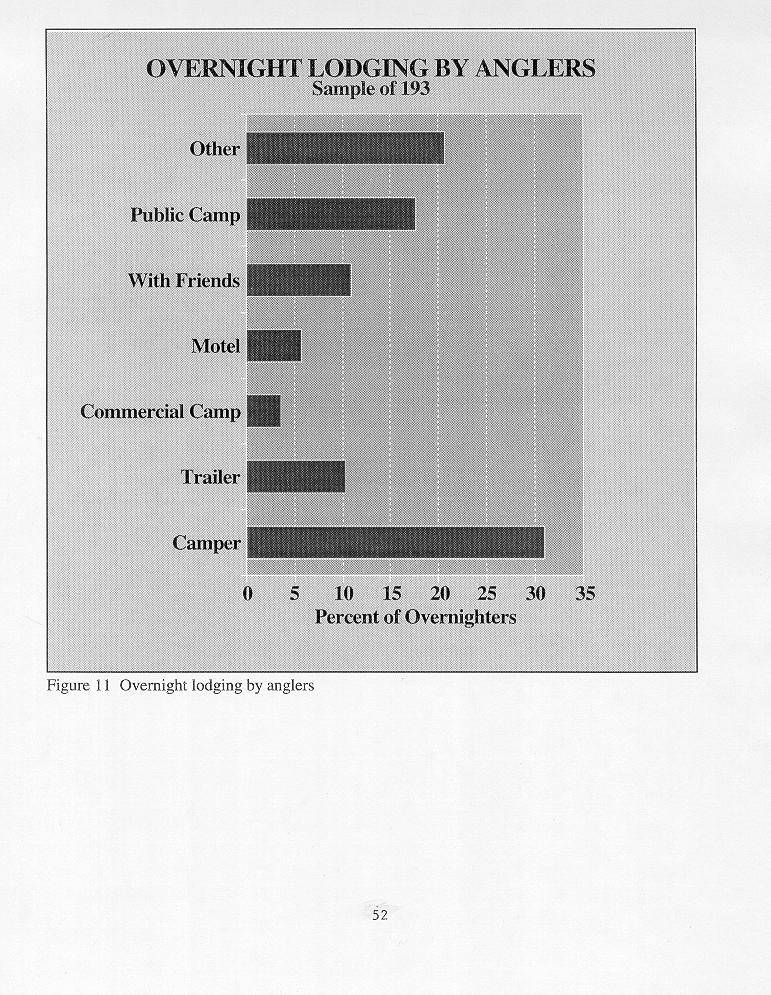
58