The seasonal variation of the upper layers of the South China Sea (SCS) circulation and the Indonesian through flow (ITF): An ocean model study

Transcription

1 The seasonal variation of the upper layers of the South China Sea (SCS) circulation and the Indonesian through flow (ITF): An ocean model study The MIT Faculty has made this article openly available. Please share how this access benefits you. Your story matters. Citation As Published Publisher Xu, Danya, and Paola Malanotte-Rizzoli. The Seasonal Variation of the Upper Layers of the South China Sea (SCS) Circulation and the Indonesian through Flow (ITF): An Ocean Model Study. Dynamics of Atmospheres and Oceans 63 (213): Elsevier Version Author's final manuscript Accessed Sun Jan 28 2:51:51 EST 218 Citable Link Terms of Use Detailed Terms Creative Commons Attribution-NonCommercial-NoDerivs License

2 1 2 The Seasonal Variation of the Upper Layers of the South China Sea (SCS) circulation and the Indonesian Throughflow (ITF): An Ocean Model Study 3 4 Danya Xu 1 and Paola Malanotte-Rizzoli Center for Environmental Sensing and Modeling (CENSAM) Singapore-MIT Alliance for Research and Technology (SMART) 1 CREATE Way, #9-3 CREATE Tower, Singapore Department of Earth, Atmospheric and Planetary Sciences Massachusetts Institute of Technology Cambridge MA 2139 USA Corresponding Author: Danya Xu danyaxu@smart.mit.edu Phone:

3 27 Abstract The upper layer of the South China Sea (SCS) circulation and the Indonesian Througflow (ITF) are simulated by using a high resolution Finite-Volume Coastal Ocean Model (FVCOM). Forced by two climatological periods of 6s and 9s which are the decadal averaged simulation results of a global circulation model MITgcm from 196 to 1969 and 199 to 1999 respectively to represent pre-warming and warming stages, the seasonal varied upper layer wind driven circulation of the SCS and ITF are successfully simulated. The seasonal variability of the circulation, thermal structure, the volume transport through the Southeast Asian maritime regions are estimated based on the model output. The model results are in good agreement with the available observational data. Numerical experiments shows the upper layer circulation of the SCS are primarily driven by the monsoon winds and reverse its directions with the alternative changing prevailing wind directions. The averaged SCS circulation in 9s is weaker than 6s due to weaker monsoonal winds. But the 9s ITF is stronger than 6s is caused by the greater Sea Surface Hight (SSH) difference between the western Pacific and the eastern Indian Ocean. The southward ITF can be blocked by South China Sea Through Flow (SCSTF) the at the Makassar Strait in upper 5m during boreal winter. Part of ITF water feed SCSTF flow into the SCS through Karimata Strait during summer. The SCSTF exports about 1.4 (2.) Sv SCS water annually into the Indonesian Seas through the Karimata (Mindoro) Strait. The SCSTF play an important role in regulating the volume transport and water property of the ITF western branch. The annual averaged volume transport of the ITF inflow (flow through Makassar and Lifamatola straits) is about 15 Sv which is very close to the long-term observations. The ITF outflow (flow through Lombok, Ombai and Timor stratis) is about 2 Sv greater than ITF inflow due to the uncertainty of the water passage of the eastern branch of the ITF inflow through Lifamatola 2

4 Strait. Both the Simple Ocean Data Assimilation (SODA) reanalysis data and model indicate the difference of the sea surface temperature (SST) and thermal structure of shallow shelf region of the SCS between 9s and 6s showing apparent warming signal, this is agree with global upper ocean heat content warming trend (Levitus et al, 29). The difference of decadal averaged NCEP net heat flux between warming stage (9s) and pre-warming stage (6s) shows the ocean obtain less heat both at the upper stream of the SCSTF (2N where Pacific water enters through Luzon Strait) and the downstream of the SCSTF (Karimata Strait) during 9s, which demonstrate that the warming of the SCS is local and not due to conduit of warmer waters from the Pacific Keywords: The South China Sea, Indonesian Through Flow, Circulation, Volume Transport, Thermal Structure. 63 3

5 63 1. Introduction The Southeast Asia Maritime Continent comprises the South China Sea (SCS), the Indonesian Seas (IS) and the complex system of currents known as the Indonesia Through Flow (ITF). The geometry of the region and the bathymetry are shown in Fig. 1a. An extensive number of investigations have been devoted to the ITF, one of the most important pathways in the water exchange between different ocean basins and the major conduit of equatorial Pacific waters into the Indian ocean, of the order of 1-15 Sv ( 1 Sverdrup = 1 6 m 3 /sec). The ITF has since long been recognized as playing an important role in the world s climate (Gordon and Fine, 1996). It transmits the El Nino-Southern Oscillation (ENSO) signal from the Pacific to the Indian Ocean via changes in the internal energy transport (Tillinger and Gordon et al, 21) and affects the Indian monsoon (Gordon, 25). Extensive observational studies have been focused on the ITF in the last decade, in particular during the International Nusantara Stratification and Transport (INSTANT) program, showing that 8% of the flow from the Pacific to the Indian Ocean occurs in the Makassar strait (Gordon et al, 28, 21). The Makassar strait (sill depth ~ 68 m.) together with the deep Lifamatola passage (sill depth ~ 2m.) are the entrance points of the ITF from the Pacific. The exit points into the Indian ocean are the Lombok, Ombai Timor and Torres straits (Fig. 1a and 1b) Many studies have been focused on the South China Sea (Fig 1a), one of the largest semienclosed marginal sea in the world. It is connected in the North to the western Pacific through the Luzon strait, deep ( ~ 2,7m. ) and wide ( ~ 3 Km.), and also to the East China Sea through the shallow Taiwan strait ( < 1m. ).The SCS in the south connects to the Sulu and 4

6 84 85 Java seas through the Mindoro ( ~ 4m.) and Karimata ( < 5 m. ) straits. All the straits are marked in Fig.1a and 1b Recently however the SCS has been shown to play a major role in the volume and heat exchanges among the various Indonesian seas, crucially affecting the ITF itself. On the basin average, the SCS absorbs heat from the atmosphere in the range from 2 to 5 Watts/m 2 ( Qu et al, 29). It is also a recipient of heavy rainfall with an annual mean value of.2-3 Sv ( Qu et al., 29). For the long term average distribution of properties, the heat and fresh water gains can only be balanced by horizontal advection. The SCS transforms the cold, salty water of northwest Pacific origin inflowing through the northern Luzon strait into warm fresh water out-flowing through the Mindoro and the shallow southern Karimata straits (Qu et al., 2, 29; Fang et al., 29; Du and Qu, 21). This circulation is called the South China Sea Through Flow (STSTF) and has been shown to actually oppose the ITF in the surface layer of the Makassar strait during winter. The circulation here is the superposition of the southward-flowing ITF in the thermocline layer and the northward-flowing SCSTF at the surface. For an excellent review of the phenomenology, major properties and importance of the SCS for climate see Qu et al (29) The SCS circulation and seasonal variations were first interpreted as the response to the forcing of the seasonal Asian monsoon in the pioneering study by Wyrtki (1961). Successive studies (Shaw and Chao, 1994; Qu, 2; Xue et al., 24; Gan et al., 26; Fang et al., 29) confirmed this explanation emphasizing also the importance of Kuroshio intrusions into the sea through the Luzon strait. Wyrtki again (1961,1987) first explained the existence of the ITF as due to the pressure difference between the Pacific and Indian oceans. Contrary to Wyrtki s pressure gradient theory, Mayer et al. (21), Mayer and Damm (212) using nested numerical 5

7 model simulated the 4 year variation of ITF, numerical simulations showed the ITF to exist even when the pressure gradient heads from the Indian to the Pacific ocean, they also suggest that Makassar strait throughflow is a distinct current which is an extension of west boundary current. Modeling studies of the South East Asia region fall within two categories, global and regional ones. In the pioneering investigation of Metzger and Hurlburt (1996), a reduced-gravity version of the global Navy layer model was used to study the coupled dynamics of the SCS, the Sulu sea and Pacific ocean. Tozuka et al. (27) studied the seasonal and interannual variations of the ITF by comparing two numerical simulations with and without the SCS, again with a global model. They showed the volume and heat transports of the ITF to increase significantly when closing completely the SCS, thus demonstrating the crucial importance of the latter one for the dynamics and balance of properties in the Indonesian seas. Regional, high resolution modeling studies (Shaw and Chao, 1994; Xue et al., 24; Gan et al., 26) on the other side focused on the SCS alone The global modeling studies suffer from the serious limitation of having relatively coarse resolution ( > ½ degree ) and a very smooth topography. They cannot therefore resolve adequately the numerous, narrow and often very shallow straits connecting the different seas. Hence, they cannot simulate sufficiently realistic ITF and SCSTF transports. The regional modeling studies, even though endowed with high resolution, focusing on the SCS alone, cannot reproduce the crucial interactions between the SCSTF and the ITF. In this study we aim to overcome both limitations. We have at our disposal the global MIT climate model, comprising an ocean and atmospheric components among others. A five decades-long simulation is available to us for the period We have embedded in the global MIT OGCM a regional, very high resolution model, the Finite Volume Coastal Ocean Model (FVCOM). The FVCOM 6

8 variable grid covers an extensive region in both the western Pacific and eastern Indian oceans, the entire SCS and ITF system with all the straits interconnecting them finely resolved. The resolution changes from ~ 1 Km at the open Pacific and Indian boundaries to ~ 5 Km. in the straits and over the steep continental slopes, as shown in Fig. 1b. The open boundary conditions and surface forcing functions are provided to FVCOM by the MIT global ocean and atmosphere GCM output. 135 We have three major objectives in the present study ) We want to reconstruct the wind-driven circulation of the SCS and IS and its seasonality induced by the dominant monsoon system. Focusing on both the SCSTF and ITF, we want to provide quantitative evaluations of the transports through all the straits interconnecting them, hence of their interactions. Whenever possible, we compare these transports to the available observations thus assessing the realism of the simulations. 2) We want to reconstruct the horizontal thermal structure of the SCS, its seasonal evolution and the properties of the stratification especially on the shallow southern Sunda shelf. We assess the modeled thermal structure against the reanalysis of the SODA dataset (Carton et al., 2). 3) Having five decades of global simulation from the MIT ogcm, we want to follow the evolution of both the wind-driven circulation and thermal structure of the SCS from the 6s to the 9s. We therefore choose the two decades and simulating the climatology of the two decades, comparing them and again comparing the modeled thermal structure with the SODA climatologies for the two decades. 7

9 To the best of our knowledge, objectives 2 and 3 have not been previously addressed. The paper is organized as follows Section 2 presents the model used in this study: the MIT global climate model and the regional FVCOM. The model configurations are discussed and details are given of the approximations and parameterizations used. The overall construction of the numerical experiments is presented. Section 3 focuses on the wind-driven circulation, exchanges between the different sub-basins through the interconnecting straits, evaluation of the straits transports and comparison with the available observations. The differences between the wind-driven circulations of the 6s and 9s are also explored. Section 4 is devoted to the evaluation of the horizontal thermal structure and vertical stratification of the shallow shelf of the SCS, its seasonal evolution and the changes between the 6s and 9s assessed against the analogous changes in the SODA reanalysis. Finally, in section 5 we summarize the major findings, deficiencies in the results obtained and prospects to correct them in future research Model Configuration and Experimental Set-up We use two models in the simulations, a global OGCM with course horizontal resolution and a regional model covering the domain of Fig. 1b in which the horizontal resolution can be increased in the narrow straits and over steep continental slopes that require a more accurate representation of vertical dynamical processes The global model is part of the MIT Integrated Earth System Model, specifically the component designed to simulate climate processes. It comprises the ocean GCM, a primitive equation, three-dimensional, hydrostatic, z-level model with the resolution of 2.5 o x 2 o in 8

10 longitude and latitude respectively and 22 vertical levels (layer thicknesses ranging from 1 to 765 m.). It includes a prognostic carbon model. The atmosphere is represented by a statisticaldynamical two-dimensional model (zonally-averaged over land, ocean and sea ice) with a 4 o resolution and 11 vertical levels. Land, sea ice and active chemistry models are also included. The wind stresses used in the global simulations are not provided by the atmospheric model but by the NCEP reanalysis ( Kalnay et al., 1996) for the simulation period The heat and moisture fluxes, on the other side, are provided by the two-dimensional atmosphere. Being zonally averaged, the longitudinal dependence of the fluxes is reconstructed through a spreading technique in which the total heat flux Q(y) is modified by adding to it the term dq/dt*δt(x,y) where ΔT is the difference between the local temperature and the zonal mean. Like most ocean/atmosphere coupled models, the ocean SST suffer from the well known climate drift problem, i.e. when forced by the atmospheric fluxes alone they drift away from the present climate. A flux correction is therefore applied to the surface temperatures and salinities by restoring them to the Levitus climatology through a nudging term. The complex spin-up procedure of the MIT gcm can be found in Embedded in the global MITgcm with one-way coupling is the regional FVCOM developed by Chen et al.(23,26b). FVCOM is an unstructured grid, finite-volume, threedimensional, free-surface primitive equation model. FVCOM solves the momentum and thermodynamic equations using a second-order, finite-volume flux scheme that ensures mass conservation on the individual control volume as well as the entire computational domain ( Chen et al, 26 a,b).the Mellor-Yamada level 2.5 turbulent closure scheme is used for vertical eddy viscodity and diffusivity ( Mellor and Yamada, 1982). The Smagorinsky turbulence closure is 9

11 used for horizontal diffusivity ( Smagorinski, 1963). For details see FVCOM has been widely used in many different coastal oceanic simulations. FVCOM configured for the SCS model grid shown in Fig. 1b. As evident, the model domain covers the entire SCS and Indonesian archipelago, including large sections of the western Pacific and eastern Indian oceans. The open eastern and western boundaries have purposely been chosen to be in the two oceans interior, far away from the SCS and Indonesian Through Flow, object of the present simulations. The domain covers all the ITF pathways, with its inflow and outflow straits marked in Fig.1b. The straits are well resolved by the variable mesh of the grid. The horizontal resolution varies from ~ 5 Km. in the straits and over the continental slopes; to 18 Km. in the shallow regions such as the SCS southern Sunda shelf, increasing to ~ 15 Km. at the open boundaries. The model is configured with 31 vertical sigma levels with higher resolution at the surface and coarser at depth, providing a vertical resolution of < 1 m. in the surface boundary layer on the shelves and ~ 1 m. in the open ocean. The real topography of ETOPO5 is interpolated to the model mesh with the maximum depth of ~8, m. in the Philippine trench, as shown in Fig. 1a. The minimum water depth is set at 1 m Ocean-only simulations also suffer from the climate drift problem, in which the simulated SST drifts away from the present climatology. As in the MIT ogcm, a flux correction is applied restoring the SST to the observed climatology as in Ezer and Mellor (1997) and, more recently, in Gan, (26). In fact the MIT heat fluxes, reconstructed through the spreading technique, are not only very coarse resolution, needing to be further interpolated to the grid of 1

12 Fig. 1b, but also incompatible with the SST simulations of FVCOM as proved by the SST drift. Again, we correct the fluxes through a nudging term: 216 τ h (T*-T) Appended to the prognostic temperature equation, where T*(x, y) is the monthlyaveraged surface temperature provided by the SODA reanalysis (Carton et al, 2). Differently from Ezer and Mellor (1997), the nudging coefficient τ h is not constant but depth-dependent. τ h linearly decreases from.2 in the shallow regions to.1 when the depth (D) reaches 3,m. and remains fixed to.1 for D> 3, m. With this formulation in the deep ocean the nudging term is negligible and the SST is determined by the atmospheric heat fluxes and horizontal/vertical dynamical processes. In the shallow regions, where the surface heat flux are most important for the heat budget, the SST, is basically determined by the SODA dataset. Also, as in Gan ( 26), we include only temperature in the simulations. Our focus is on the winddriven circulation of the SCSTF/ITF and on the thermal structure of the upper ocean averaged over a decade, specifically the two decades of the 6s and 9s separately. Over this short time scale, the long-term, centennial evolution of temperature and salinity necessary to balance through horizontal advection the surface heat (warming) and moisture (freshening) fluxes cannot be simulated. Also, on the decadal time scale, temperature is the more dynamically important variable while salinity behaves more like a passive tracer. As a further remark, decadal simulations cannot reconstruct the more-than-centennial evolution of the deep thermal structure and of the associated thermohaline circulation. The deep stratification is hence determined by the initial condition provided by the MIT OGCM. The differences in the average climatologies of the 6s and 9s reconstructed by the regional simulations are therefore due to the differences 11

13 between the two decades in the surface forcing functions, wind stresses and heat fluxes over the shallow regions only. As over the shallow regions the SST are strongly constrained by the SODA reanalysis, their differences will correspond to the SST-SODA differences between the 6s and the 9s. The subsurface thermal structure in the shallow regions will be determined by vertical diffusion in the surface layer For the two decades of the 6s and 9s, the input from the MIT OGCM to the regional domain is constituted by the decadal weekly averages of i) sea level; ( T,S) and (u,v) at all levels at the open boundaries ii) solar radiation and net heat flux at the surface iii) NCEP weekly averaged wind stresses We spin up the regional domain with the perpetual year of the average 6s and 9s. After a 14 year spin-up, the wind-driven circulation has equilibrated as evident from the evolution of the total kinetic energy (spin-up time ~three years, not shown). The thermal structure in the upper layer, above 1 m., also reaches equilibrium in roughly the same time as evident from the temperature evolution at the sigma-levels (not shown). The initial condition for spin-up is the first week in January of the two decades. Circulation and thermal structure properties are diagnosed and quantified in the one-year after spin-up. Particular attention had to be given to the pressure gradient determined by the sea level distribution at the two open boundaries in the Pacific and Indian oceans respectively. The very coarse horizontal resolution of the MIT OGCM sea surface heights (SSH) provide unrealistic geostrophic currents and unrealistic transports at the open boundaries, especially crucial along the eastern Pacific side with the inflows/ outflows of the tropical Pacific currents, such as the North Equatorial Counter Current (NECC), the North 12

14 Equatorial Current (NEC) and the northernmost Kuroshio. These boundary pressure gradients compete with the monsoon driven circulation in the interior of the regional domain, and can actually reverse it. An extensive sensitivity study, which we do not report in detail, was therefore carried out adjusting the boundaries SSH to reproduce realistic values of the tropical Pacific currents transports and of their patterns. The Indian boundaries SSH did not prove crucial as they mostly constitute exit points of the interior ITF flow Finally, tidal forcing is not included either in the MIT OGCM or in FVCOM. Tides are not simulated in global circulation models, devoted to study the ocean circulation and in fact tidal models are rather different form OGCM (see for instance Zu et al., 28). Tides, being periodic phenomena, are dynamically irrelevant for the general circulation. Their only effect is mixing and energy dissipation over the shelves, effect which is parameterized through bottom and lateral friction The SCS Wind Driven Circulation Monsoonal Wind Stress The SCS and Indonesian Seas are under the control of the fairly complex monsoon wind system. Figure 2. shows the decadal averages of the National Centers for Environmental Prediction (NCEP) winter/summer wind stress (N/m 2 ) of the 6s, Fig.2a and 2b, 9s, Fig.2c and 2d, and their difference (9s-6s), Fig.2e and f respectively. In the winter season (DJF), the Northeast (NE) monsoon wind dominates over the SCS and its magnitude reaches the maximum value (>.2 N/ m 2 ) along the northeast-southwest diagonal axis of the SCS basin. The wind stress magnitude gradually decreases from the SCS interior to the land-coasts and changes direction 13

15 over the ITF system, becoming mostly zonal and eastward. The NE Indian monsoon has a weaker magnitude (~.5 N/ m 2 ) and converges with the Southwest (SW) Australian monsoon over the eastern Indian Ocean equatorial region. The Malaysian-Australian monsoon is eastward from the Java sea to the western Australian coast. During Summer (JJA), the Australian monsoon keeps a northwestward direction and intensifies in magnitude reaching ~.15 N/ m 2. Both the Asian and Indian monsoons reverse from NE to SW. The magnitude of the Asian monsoon over the SCS is weaker (.5 to.8 N/ m 2 ) compared with the Indian and the Australian monsoons (~.15N/m 2 ). The Malaysian-Australian monsoon reverses with a magnitude of ~.2N/m 2 greater than its winter counterpart. The Spring (MAM) and Fall (SON) are the monsoon transient seasons with relative small wind speed (not shown) Compared to the 6s, (Fig.2 a & b), the wind stress field of the 9s (Fig.2 c & d) shows a very similar pattern, but there are noticeable differences between the two as shown in Fig. 2 e-f. Overall, the differences (9s-6s) both in Winter and Summer are opposite to the general wind direction in that season (NE in Winter and SW in Summer), indicating that the 6s winds are stronger than the 9s.This is particularly clear for Summer, Fig. 2f, with the greatest difference reaching a maximum of ~.5 N/m 2 over the SCS interior and NE Indian ocean. The Winter difference, Fig. 2e, is more complex, showing a small cyclonic gyre in the southern half of the SCS, indicating a stronger cyclonic tendency in the 9s. In the northern SCS the 6s Winter wind stress is again stronger than in the 9s This picture is confirmed by the wind stress curl evaluated for the two seasons and the two decades. Fig 3 shows the Winter/Summer curls for the 6s, Fig 3a and 3b, and for the 9s, Fig 3c and 3d, respectively. All the patterns show the line of zero wind-stress curl crossing the 14

16 SCS along its longest diagonal axis in northeast to southwest direction. The curl consists of two lobes of opposite sign on either side of the zero line. In the Winter season a cyclonic ( positive) curl is present over the eastern side and an anticyclonic ( negative) one on the western side. The pattern is reversed in Summer, with the eastern side now characterized by a negative curl and the western side by a positive one. The two regions of opposite curl show the presence of various centers of high intensity. In Winter 6s two strong centers of ~ 2.5 x 1-7 N/m 3 are present in the northern and southern SCS separated by a third, weaker cyclonic center. In Winter 9s the southern center is more intense reaching a maximum of 3 x 1-7 N/m 3 and the northern one weakens to 1.5 x 1-7 N/m 3, confirming the patterns of Fig.2e indicative of a stronger southern cyclonic tendency. The western, anticyclonic region has a weaker negative curl in the 9s than in the 6s The reversed Summer pattern shows consistently weaker curls in the 9s than in the 6s, both in the cyclonic and anticyclonic regions. The difference in the centers intensity however does not exceed +1 x 1-7 and -.5 x 1-7 N/m 3, of the same order as the Winter ones. The NCEP curl patterns of Fig 3 are very similar, both in shape and intensity, to the curl patterns of Qu (2) for the Hellermann and Rosestein (1983) climatology; and to the patterns of Liu et al (21); Xue et al (24) for the COADS climatology. This similarity indicates that the differences between the two decades in the NCEP winds do not reflect long-term average trends but are rather a manifestation of interdecadal variability around a stable climatology. We therefore expect to find similar wind-driven circulations in both decades, with minor differences due to decadal variability SCS Seasonal Circulation 15

17 Two competing forces drive the circulation in the upper layers of the Southeast Asia Maritime Continent, the wind stress and the pressure gradients determined by the SSH distribution at the open boundaries. The crucial boundary is the one in the eastern Pacific where the ITF inflow is generated. In the SCS the dominant driving force is the wind stress and the surface circulation reflects the seasonality of the monsoon system. The circulation reverses from Winter to Summer, with a net cyclonic tendency in Winter and an anticyclonic one in Summer, reflecting the corresponding seasonal wind curls of Fig.3. This is evident in Fig.4, showing the Winter surface currents, Fig. 4a, and the Summer ones, Fig. 4b, for the 6s. These circulation patterns are consistent with previous modeling results ( Metger and Hurlburt, 1996; Xue et al., 24; Gan et al., 26; Fang et al., 29) In Winter, Fig.4a, western Pacific water enters the SCS through the northern Luzon strait, merges with the coastal water of the northern shelf and turns southward when reaching the eastern Vietnam coast. This western boundary current bypasses the southern Vietnam coast splitting into two branches. A small branch turns northwestward and flows into the Gulf of Thailand. The major current flows southward out of the SCS through the Karimata strait, thus becoming part of the Pacific to Indian throughflow. In the Karimata strait the current reaches a maximum speed of.7 m/sec. This SCSTF in Winter proceeds eastward in the Java sea blocking the southward flow of the ITF in the Makassar strait. The surface circulation reverses in Summer, Fig.4b. After entering the SCS through the Karimata strait, a small part of the SCSTF turns northwestward into the Malacca strait, while the major SCSTF branch turns eastward to form an anticyclonic gyre in the southern part of the basin. The northern limb of this gyre forms a broad eastward current detaching from the Vietnam coast. In the northern SCS the current flows northeastward out of the SCS through the Luzon and Taiwan 16

18 straits into the Pacific ocean. Due to the weaker wind speed, (Fig. 2), the Summer surface currents are also generally weaker than the winter ones We do not show the corresponding circulation patterns for the decade of the 9s as they are extremely similar to those of the 6s and no differences are apparent upon a simple visual inspection. Rather, figs. (4c,d) give explicitly the difference in currents between the 9s and the 6s. It is evident that the circulation differences are highly correlated with the wind differences between the two decades, Fig 2e, f. In Winter, Fig.4c, the difference (9s-6s) shows a broad cyclonic gyre in the southern SCS, reflecting the stronger cyclonic tendency in the 9s winds. The current difference in this gyre is about.1 m/sec. The differences in the remainder of the SCS are very small (<.1m/sec), indicating an overall stable climatology of the surface Winter circulation In Summer, Fig.4d, the Karimata strait surface velocity difference is southward and reaches.1 m/sec, indicating that the 9s Summer northward current is smaller than in the 6s. The (9s-6s) differences in the surface circulation are overall reversed with respect to the Summer current directions, reflecting the weaker currents of the 9s. The surface circulation patterns of the two decades and their differences are reproduced in the patterns at 5 and 1 m. depths. We therefore present only the results for the 6s as they are representative of a stable wind-driven circulation in the SCS with only minor differences due to decadal variability The currents at 5 m. depth are presented in Figs.5a,b. Due to the shallowness of the Karimata strait ( < 5m. ), the SCS circulation is closed in the basin interior at this and at deeper depths. Therefore below 5 m. the SCSTF and ITF do not interact any longer. The overall mass balance in the SCS can only be through inflows/outflows in different vertical layers in the Luzon 17

19 and Mindoro straits. The major difference in the 5m. patterns is that in Winter, Fig. 5a, a branch of the Kuroshio intrudes into the SCS through the Luzon strait forming a loop flow. This Kuroshio intrusion proceeds westward at a speed of ~.15 m/sec along the northern continental slope. Combined with the northern part of the recirculation gyre, it intensifies at the western coast flowing subsequently southward along Taiwan and reaching the southwestern corner of the SCS, with a maximum speed of.2 m/sec at the northern Sunda shelf. Two cyclonic gyres are located in the northern and southern basins, with an anticyclonic, weaker one between them. In Summer instead, Fig. 5b, the Kuroshio bypasses the Luzon strait and flows northeastward. There is a cyclonic gyre over the northern half of the SCS and an anticyclonic one in the southern half, the southern boundary of the latter located over the Sunda shelf. The anticyclonic eddy located at the eastern shallow shelf off Malaysia Peninsula seems confirmed by the monthly mean TOPEX/Poseidon SSH anomaly data by recent numerical simulations (Tangang et al., 211) The circulation at 1m. depth for the 6s is shown in Fig. 6a,b., and is consistent with the pattern at 5 m. but confined to a smaller basin. It is also consistent with the results of Gan et al. (26). In Winter, Fig. 6a, most of the Kuroshio water returns to the Pacific ocean at northern part of Luzon strait, part of Kuroshio water still present as a western boundary current inside the SCS. Also present is the northern cyclonic eddy west of Luzon, consistently with Qu s climatological observations (Qu, 2). Wang et al (28) s numerical model suggested that the winter mesoscale eddies in the eastern SCS can only be resolved in high resolution local wind forcing. Driven by NCEP wind data without orographic wind jets resolved in Luzon area, the mesoscale eddies still present in our simulation. The mechanisms of winter eddy genesis in the eastern SCS need further investigation. In Summer, the semi-enclosed SCS circulation consists again of the two opposite gyres observed at 5 m., albeit smaller and weaker, Fig. 6b. A 18

20 northeastward jet (7-8 cm/sec) veers off central Vietnam and separates the northern cyclone from the southern anicyclone, which are consistent with the ADCP observations of Li and Wu (26). The life cycle and forming mechanism of this summer dipole circulation structure off central Vietnam coast was studied by Wang et al (26) using an idealized model. Numerical experiments indicated that the offshore wind jet determined the magnitudes and the core positions of these two eddies ITF Seasonal Circulation The local wind system over the maritime continent is more complicated compare with the SCS which not only include the Asian Monsoon but also Malaysian-Australian Monsoon and Western Australian Monsoon (Fig.2 and 3). Driven by this complex monsoon wind system, the winter and summer surface circulation in both 6s (Fig.4 a-b) and 9s (not shown) in the Indonesian seas show the same flow pattern: reverse its direction but this phenomenon only confined in the surface layers. In winter, south Pacific surface water enters the Sulawesi Sea then continually flows into the Makassar Strait, this western branch of the ITF is converged with the northward SCSTF at south end of the Makassar strait. The eastern branch of the ITF enters the Malucca sea flow through the Lifamatola strait. Both of these two branches of the ITF are blocked by the eastward SCSTF and no apparent pacific water enters Indian Ocean at the surface. In summer (Fig.4b), the surface flow of Makassar strait turns to northward. Driven by westward wind, the surface Indonesian seas flow drift to northwest, Flores sea and Banda sea water transport to the Indian Ocean through the ITF outflow passages: Lombok, Ombai and Timor straits. Part of the water from southern end of the Makassar Strait turn southwest and join into the westward inflow of the SCSTF. The complete pathway of the ITF is hard to be identified due 19

21 to strong surface wind driven circulation. This seasonal alternative changed pattern of the surface Indonesian maritime flow is consistent with Gordon s (25) review and INSTANT observations Below the surface (5m and 1m, Fig5-6), the ITF is a relative consistent flow sourced from the tropical Pacific Ocean bypass the complex water passages of the Indonesian Seas and flow into the Eastern Indian Ocean with less seasonal variation and keep the same flow direction. At western Pacific low latitude region (7-12 o N), the westward NEC split into northward Kuroshio and southward Mindanao Current (MC) when reaching Philippine east coast. The southward MC and some SCS water from the Mindoro strait are the origin of the ITF. The western branch of the ITF forms a steady southward jet stream with a maximum speed over.5m/s at 5m due to the funnel shape of the Markassar strait. The velocity profiles of the INSTANT observation (Gordon et al, 28) also demonstrate this character of the subsurface current intensification of the ITF in Makassar strait. A minor part of ITF flow through the Markassar Strait directly enters Indian Ocean through the Lombok Strait. In the winter, part of the ITF outflow at Lombok is from the SCSTF water. This is consistent with Gordon s (25) conclusion from the water property analysis. In general, the speed of the southward flow at the Lombok Strait can reach.15m/s, about two third of the summer outflow velocity (Fig.5b, 6b). The major part of western branch of ITF from the Makassar Strait turns eastward, crosses the Flores Sea and flows all the way to the Banda Sea, then turns sharply southwestward at eastern Timor, flows into the eastern Indian Ocean through the Ombai Strait and the Timor Strait. Once enters the East Indian Ocean, the current flow toward west hugging tightly the southern Java coast. The ITF pathway can be clearly distinguished from the subsurface layer of the velocity field (Fig5-6). Especially during summer, even the wind (Fig.2) and the surface current at Flores Sea (Fig.4) is westward, but the subsurface current flow against the wind direction to form the 2

22 ITF flow jet. Open boundary of sea level difference between two ocean basins determined this flow. The flow pattern of the main stream of the ITF at 1m (Fig 6 a-b) and 5m (Fig 5 a-b) are quite similar and the current speed of ITF maintains around.3m/s The circulation differences of 9s and 6s around ITF region shows the eastward currents from the Flores sea to the Banda sea are apparently intensified in 9s from surface (Fig 4c-d) to 1m (not shown). This intensified current reinforces the ITF outflow transport through Ombai and Timor straits during 9s. The current speed difference can reach.15m/s at the surface and.5m/s at 5m and 1m. Even the overall monsoon wind during the 9s is weaker than 6s, but stronger ITF current during 9s is a result of a greater seal level difference between Pacific Ocean and Indian Ocean in 9s than in 6s (not shown) The modeled flow pattern of the ITF region agrees rather well with the deduced conceptual ITF routes based on long-term observation (Wyrtki, 1961, 1987; Gordon and McClean, 1999; Gordon et al, 21; Sprintall et al, 29). The model simulation indicated that unlike the SCSTF, the overall circulation of the ITF around the Indonesian Seas (Fig.4-6) is primarily controlled by the open boundary rather than the monsoon winds. The sea level difference between the Pacific and Indian Ocean generated by the pressure gradients of the open boundary is the major driving force of the ITF (Wyrtik, 1987). However, the monsoon winds can influence the surface circulation of the ITF significantly Volume Transports and Comparison with Observations In order to quantify the interocean transports and evaluate the interaction between the SCSTF and the ITF, the volume transports through the water passages are calculated from 21

23 456 F v =! V da (1) A n The total transport through each transect is the sum of the product of the velocity component perpendicular to the transect (V n ) and the area element da on the transect. Since the model grid is an unstructured triangle mesh, we interpolate all variables on the line transect crossing the considered strait. The transects of the SCSTF and the ITF passages are labeled in Fig1b Figure 7 shows the annual, summer (JJA)/winter (DJF) mean transports and the evolution of the monthly averaged volume transport through the SCSTF passages (Luzon and Karimata Strait, fig 7a and 7b, Mindoro and Sibutu Strait, fig 7c and 7d), the ITF inflow (Makassar and Lifamatola Strait, fig7e and 7f) and the ITF outflow (Lombok, Ombai, Timor and Torres straits, fig 7g-i) for both 6s and 9s. There is an obvious relationship between the Luzon strait transport (Fig 7a) and the prevailing monsoon. Westward Ekman transport (negative) apparently enhances the Kuroshio intrusion during Winter. The intrusion of the Kuroshio through the Luzon Strait is the upstream end of the SCSTF and the Luzon transport can increase from 4.6 Sv (x 1 6 m 3 /s) in Summer time to ~ 7. Sv during Winter giving an annual average value ~ 5.6 Sv. This value is in very good agreement with Tian et al (26) s hydrographic observation (6±3 Sv). Because of the lack of synoptic observations, the existing estimates of the Luzon transport are based on the upper layer dynamic calculation (Wyrtki, 1961; Qu et al, 2) and numerical models (Metzger and Hurlburt, 1996; Xue et al, 24; Qu et al, 26; Tozuka et al, 27; Fang et al, 29). The estimated Luzon annual transport varies from.1 to 8. Sv with great uncertainty (Fang et al, 29). Our numerical simulation is very close to the mean of these estimates (~ 4.5 Sv). The 6s and 9s Luzon transports basically the same. 22

24 In the 6s, about 1.4 Sv annual net SCSTF transport leaves the SCS through the Karimata Strait and enters the Java Sea, in which the outflow (inflow) occurs during Winter (Summer) at about 3.6 (1.1) Sv. Compared with most of the previous numerical estimates, the net yearly transport through the Karimata Strait is larger. For instance, the annual mean transport is.6 Sv in Metzger et al (21) s simulation. Recently, however, Fang et al (21) deployed 2 velocity moorings in Karimata from 27 to 28. They found that the Winter maximum surface current can reach 7cm/s, with the bottom velocities not less than 2cm/s. They estimated the Winter transport to be of 3.7 Sv. In our simulation the Winter outflow from Karimata is ~ 3.6 Sv., in excellent agreement with the measured value. Unfortunately, Fang et al. did not retrieve data during Summer. The time series of the Karimata transport (Fig 7b) shows the Summer inflow to be smaller than the Winter outflow which is consistent with the Summer monsoon being weaker than Winter one. As the Karimata strait is very shallow, its transport is controlled by the wind. Consistently, as the Summer monsoon in the 9s is weaker than in the 6s, the 9s Karimata Summer inflow is about half that of the 6s. Overall, our model estimates of the SCSTF inflow through Luzon and outflow through Karimata are in very good agreement with the best available observational estimates Besides Karimata, Mindoro strait is another important passage for the SCSTF to export Pacific origin water into Indonesian Seas. This branch of the SCSTF combined with westward Pacific water through Philippine islands flow southward through Sibutu strait and finally feed into the upstream of the ITF. For both 6s and 9s, about 2. Sv SCS water enter Sulu Sea through Mindoro Strait (Fig 7c), at the same time, about 2.9 Sv water flow southward pass through Sibutu Strait and integrated into ITF (Fig 7d). These volume transport values are very close to Qu and Song (29) s estimations from satellite data (Mindoro transport is 2.4 Sv and 23

25 Sibutu transport is 2.8 Sv). The modeled seasonal variation of the volume transports of these two straits are nearly in phase: The minimum transport occurred during early spring (March), then gradually increased and reach its maximum in autumn (October). The patterns of the transport seasonal variations are consistent with Qu and Song (29). Interestingly, this seasonal variation is opposite to the ITF seasonal transport variation phase. Since these two straits contribute significant water to ITF upstream, our model indicates that the transport through Mindoro and Sibutu can regulate the seasonal variation of the ITF. Gordon et al (212) analyzed the variation of the ITF through Makassar Strait based on observation and HYCOM model simulation, they suggest the weaker Makassar Strait transport during El Nino year may due to stronger SCSTF through Mindoro Strait block the Pacific water westward supply As the circulation (Fig 4-6) shows, the basic pattern of the total ITF transport and the monthly variation of these two decades are the same but the overall ITF transport of the 9s is greater than the 6s. The modeled total ITF inflow transport is the sum of the Makassar and Lifamatola strait transport with significant seasonal variations (Fig.7e-f). The Makassar Strait is the main route of the ITF and the annual averaged transport is about 9.6 and 1.3 Sv in the 6s and 9s respectively. Tillinger and Gordon (29, 21) analyzed Makassar transport from 1948 to 27 total 5-yr variation of the SODA data and they found the averaged 6s ITF transport is smaller than 9s. From the time series of the transport (Fig 7e) a double peak seasonal variation can be observed. The southward transport gradually increases from Winter (DJF) reaching the maximum value of 11.4 Sv ( 6s) and 12.2 Sv (9s) in March, then decreases to 8.6 Sv ( 9.6 Sv) from April to June, then increases again and reaches the second peak of 11.9 Sv ( 12.1 Sv) in August. Afterwards, the transport decreases to its minimum ~ 6 Sv ( 6.5 Sv) in October and November. The smaller Makassar transport during the Winter season may be due to the strong 24

26 eastward SCSTF that blocks the southward ITF at the southern entrance of the Makassar strait in the surface layer (upper 5m). On the other side, in Summer part of the ITF turns westward to feed into the reversed SCSTF flow and into the SCS. The interaction between the SCSTF and the ITF manifests itself through this alternating blocking and feeding mechanism that regulates the ITF transport and water property exchanges. The recent published synoptic observations of the INSTANT program shows the 3-year mean Makassar strait transport to be nearly 11.6±3.3 Sv with a double peak pattern. The maximum transport occurs towards the end of the northwest (March) and southeast monsoons (August), with the minimum transport during the monsoon transition seasons (May and November) (Gordon et al, 28). Our modeled Makassar transport seasonal cycle agrees well with the INSTANT observations even though the model annual averaged transport is 1-2 Sv smaller. Numerical experiments of long term integrations of the high resolution model (Shinoda et al, 212) found that the wind is the key factor in controlling the seasonal variation of the ITF at Makassar Strait. The INSTANT observations also show the eastern routine of the ITF through the Lifamotala strait to be about 3 Sv of which 2.5 Sv is the contribution from the deep flow (125m to bottom) as upper layer observations are not available ( van Aken et al, 29). The modeled Lifamatola Strait transport is about 5.5 Sv in the 6s and 6.3 Sv in the 9s of which about half is from the surface to 125m and the other half is from the deeper flow (125m to bottom). A detailed comparison between modeled and observed values is not possible because of the lack of upper layer measurements. Combined with the Makassar transport, the modeled total ITF inflow is 15.1 and 16.6 Sv in the 6s and 9s respectively (Table 1), close to the INSTANT observation (13 Sv) and within the uncertainty range Figure 7g-i is the modeled volume transport of the ITF outflow passages (Lomok, Ombai, Timor and Torres Straits). Unlike the other two, the Lombok transport (Fig 7g) shows less 25

27 seasonal variations. Compared with the Ombai and the Timor straits, the Lombok strait is the shallowest with the sill depth at about 3m, and the narrowest width of ~ 35 km, both of which limit the transport. The 9s transport is.7-.2 Sv greater than the 6s during January to March, the remaining months being almost the same (Fig 7g). The Winter average transport is ~ 3.4 Sv and the Summer one is ~ 4.1 Sv in the 6s. Even if the annual average ITF inflow increases by 1.5 Sv from the 6s to the 9s, the Lombok transport remains the same in the two decades. The model annual average Lombok transport (3.7 Sv) is about 1.1 Sv greater than the INSTANT 3 year average value of 2.6 Sv (Springtall et al, 29). The Ombai strait is a narrow (~35 km) but deep (325m) channel connecting the Banda and Savu seas. The annual average Ombai transport (Fig. 7h) of the 9s is.6 Sv greater than the 6s. The maximum transport occurs during the monsoon seasons with the Winter (DJF) transport greater than the Summer one (JJA). This seasonal variation is consistent with the INSTANT record and the model overestimates the annual average transport by Sv (Springtall et al, 29). The largest transport difference between the two decades is in the Timor strait (Fig. 7i) with 7.8 Sv in the 9s and 6.4Sv in the 6s. The 9s transport is very close to the INSTANT observation (-7.5 Sv). The time series of the Timor transport is in phase with the Makassar one, indicating that the Timor strait is the main outflow path of the ITF. The Torres Strait is the only water channel connecting the Arafura Sea and the South Pacific Ocean. But the transport (Fig. 7j) is negligible because of the shallow water depth. The westward (eastward) flows during Summer (Winter) are less than.25 Sv and the annual average of.1 is the same in both decades. This value is very close to Metzger et al (21) s estimate of.2 Sv Overall, the modeled annual averaged total ITF outflow is nearly 16.8 Sv in the 6s and 18.9 Sv in the 9s (Table 1), with the outflow greater than the inflow by ~ 1.7 Sv and 2.3 Sv 26

28 respectively. There is a 2 Sv difference between the ITF outflow and inflow in the INSTANT observations (Gordon et al, 21). This difference can be attributed mostly to the uncertainty of the Lifamatola Passage transport estimate. Overall, considering the scarcity of observations, the model transport estimates of the total ITF inflow/outflow are in good agreement with the values shown in Table Thermal structure As stated in the introduction, one of the major objectives of this work is to reconstruct the interior thermal structure of the SCS and its evolution during four decades. To our knowledge, no previous study has focused on the SCS thermal properties. As we did for the wind-driven circulation, we contrast the two decades of the 6s ( average) and 9s ( average) having at our disposal five decades of global simulation from the MITgcm The motivation for this investigation stems from the Levitus et al. (2, 21, 25, 29). Levitus et al. (2) reported that the heat content of the world ocean from the surface through 3 m depth increased by ~ 2x1 23 Joules between the mid-5s and mid-9s representing a volume mean warming of.6 C o. This trend was attributed to the increase in greenhouse gases in the earth s atmosphere in Levitus et al. (21). More recently, these estimates have been updated for the upper 7 m. of the world ocean and discarded the unreliable XBT data for the period giving a linear increasing trend of.32x1 22 Joules/yr starting in 1969 and for the period ( Levitus et al, 29, Fig. S9). We are therefore interested in investigating if the upper layers of the SCS, and especially its southern shallow Sunda shelf, has also undergone a similar warming. According to the global average heat content of the upper 7 m. given by Levitus et al.(29), the decade belongs to the 27

29 pre-warming phase, while the decade is in the full warming phase. The two decades therefore should represent two different climatological regimes Our reference dataset for the two decades is the SODA reanalysis (Carton et al, 2) which we examine first to establish thermal trends in our domain. Figure 8 shows the temperature differences between 9s and 6s (9s minus 6s) of the SODA decadal averages during Winter, Summer and over the entire year at the surface, 15m. and 5m. in the SCS and Indonesian seas. It is clear that the 9s yearly averaged temperatures in the SCS are overall warmer than the 6s at all these three levels (Fig 8c, 8f and 8i). The highest temperature differences occur during Summer (JJA) (Fig 8b, 8e and 8h) and the warmest region is in the western part of the SCS, with the 9s ~ 1-2 o C warmer from the surface to 5m. In Winter (DJF), the temperature differences are smaller (<.5 o C), and even cooler in the northern shelf and western Luzon island (Fig 8a, 8b and 8c). The ITF region and southern Java coast actually show cooling between the 9s and 6s, especially at 5m. depth. From the SODA data, there is clear warming in the upper layer of the SCS, consistently with the global estimates of Levitus et al (29) As already discussed in section 2, we use the surface forcing and open boundary conditions from the global MITogcm multi-decadal simulation. We integrate the two climatological periods for 15 years each and examine the thermal structure of the last year of the two simulations. The modeled temperature differences between the 9s and 6s during Winter, Summer and yearly average at the surface, 15m. and 5m. are shown in Figure 9. Even with a very weak nudging coefficient, the modeled sea surface temperature differences (9s- 6s) (Fig.9a-c) are extremely similar to the corresponding SODA temperature differences (Fig.8a-c). 28

30 The warming signal is very strong in Summer (Fig.9b) and weaker in Winter (Fig. 9a) in the SCS region. At 15m, the warming trend is still detectable but the magnitude is smaller than in the SODA dataset. The warmest regions again appears in the western part of the SCS and is only 1 to 1.5 o C higher in Summer ( Fig. 9e). The 5 m. temperature difference on the other side show an overall cooling over most of the SCS even in Summer, with only a small warmer region in the western SCS with a magnitude of about.7 o C. The ITF region shows a significant cooling at 5 m. depth similar to what observed in SODA. As a conclusion, the warming trend in the SCS is well reproduced at the surface and 15 m depth but is rather weak at 5 m We focus more thoroughly on the thermal structure evolution on the shallow Sunda shelf of the SCS which should be the region mostly affected by the warming trend due to its shallowness. Two shallow sites at midway of the SCSTF are chosen to analyze the vertical temperature profile variations throughout the year. Figure 1 gives the comparison of the SODA data and the modeled monthly average temperature profiles at site T1 (red circle on Fig.1b) and T2 (red star on Fig.1b) for the 6s. The SODA data shows that both sites are well mixed from the surface to the bottom in most months of the year (Fig.1 a & b). Site T1 is located at the entrance of the Gulf of Thailand with a depth of 72m (SODA smoothed topography is 58m deep ). The coldest SST is in February with a temperature of 26.8 o C, afterwards the SST gradually increases to 29.5 o C in May. There is a weak stratification during spring (MAM), with a thermocline at ~ 2m. The bottom temperature variation is from 25 o C (May) to 27.4 o C (September). Site T2 is located at the entrance of the Karimata Strait with a depth of ~53m (SODA smoothed topography 25m ). The water column is always well mixed and no stratification is presented from January to December due to the shallow water depth. SST varies from a minimum of 27.7 o C in December to a maximum of 29.4 o C in May. The narrower temperature excursion of SST at 29

31 site T2 is due to its location closer to the equator (~.4N) with a more invariant solar radiation during the year. Figures 11 a,b show the same temperature profiles from SODA at sites T1 and T2 for the 9s. Compared to the 6s, the maximum SST of the 9s at both sites increases to 3 o C. Therefore the warming signal can also be detected at single points in the shallow shelf of the SCS The FVCOM simulated temperature profiles ( Figs 1 c,d and 11 c,d) at these two sites agree rather well with the SODA data. They also show that the 9s are warmer than the 6s. At site T1, as in SODA, a weak thermocline forms at ~ 2 m. during Spring (MAM) and the water column is well mixed during the rest of the year in both decades. The bottom temperature varies from 24.5 C o in May to 27 C o in September in the 6s and similarly from 24.6 C o in May to 27 C o in September in the 9s. At site T2, even though the real topography is more than twice greater than in SODA, the simulated temperature profile ( Fig. 1 d and 11 d) show that heat is mixed down to 5 m. during the entire year. The model simulation reproduces rather well the SODA temperature profiles in shallow water, which show considerable vertical homogeneity throughout the water column Conclusion In this paper we investigate the wind-driven circulation and the thermal structure of the Maritime Continent which comprises the South China Sea (SCS), the Indonesian Seas (IS) and the complex system of islands and straits which determine the Indonesian Throughflow (ITF), the most important conduit of tropical Pacific waters into the Indian Ocean. We use the FVCOM model in the regional configuration of Figs 1a,b embedded in the global MITgcm which provides surface forcing and lateral boundary conditions at the Pacific and Indian open boundaries. 3

32 Previous modeling studies were of two types. The global simulations suffered from the serious limitation of coarse resolution. The regional simulations, even though endowed with high resolution, focused mostly on the SCS alone, thus not including the crucial interactions between the ITF and the SCSTF. The latter one profoundly affects the ITF and even reverses the ITF in the surface layer during the Winter monsoon. In this study we overcome both limitations We have at our disposal five decades of a global simulation from the MITgcm, from 1958 to 28. From the work of Levitus, and his most recent global data analysis ( Levitus et al., 29) the global average heat content of the upper 7 m. show a linear increasing trend starting in 1969 over the entire period The decade belongs to the pre-warming phase, while the decade lies in the full warming phase. We choose therefore to simulate and contrast these two decades which represent two different climatological regimes The decadal averaged NCEP net heat flux (summation of sensible heat, latent heat, short and long wave radiation) difference between 9s and 6s (Fig. 12) shows about 2-3 W/m 2 heat gained more in the central SCS in 9s. But the ocean gain less heat both at the upper stream of the SCSTF (2N where Pacific water enters through Luzon Strait) and the downstream of the SCSTF (Karimata Strait) during 9s, this means that the warming of the SCS is local and not due to conduit of warmer waters from the Pacific and it does not reflect the large scale circulation. We have three major objectives in this study. First, we want to reconstruct the wind-driven circulation of the SCS and IS and its seasonality induced by the dominant monsoon wind system. We want to provide quantitative estimates of the transports through the straits of the SCSTF and ITF and assess them against the available observations. Second, we want to reconstruct the thermal structure of the basin and the properties of the stratification in the shallow southern 31

33 Sunda shelf of the SCS where warming trends may be more apparent. We assess the simulated thermal structure against the SODA reanalysis (Carton et al., 2). Finally, we want to compare the climatology of the two decades, the 6s and the 9s, and determine whether significant changes have occurred in both the wind-driven circulation and the average decadal stratification. To the best of our knowledge, no previous study has addressed these last two objectives Two major competing forces drive the circulation of the basin, the wind stress and the pressure gradients determined by the SST distribution at the two open boundaries of the Pacific and Indian ocean, specifically the difference in sea level between the two oceans. In the SCS the dominant driving force is the wind stress and the surface circulation reflects the seasonality of the monsoon system, reversing from Winter to Summer, with a net cyclonic tendency in Winter and anticyclonic in Summer. In the deeper layers the circulation show great spatial variability determined by baroclinicity and topographic effects, with mesoscale eddies embedded in the basin-wide circulation. Features such as the western Luzon Eddy, summer dipole off Vietnam are well reproduced in the simulation. Overall, the circulation patterns and eddy features are in good agreement with the observations and previous numerical modeling studies. The SCS circulation differences between the 9s and 6s are highly correlated with the wind stress differences between the two decades. In Winter, the (9s-6s) circulation difference reflects the stronger cyclonic tendency in the 9s wind stress curl. In Summer, the (9s-6s) difference shows weaker currents in the 9s, reflecting the weaker monsoon forcing. However, overall both the wind curls and the circulation patterns are rather similar in the two decades. This similarity indicates that the decadal differences of the wind-driven circulation do not reflect a long-term trend but are rather a manifestation of interdecadal variability around a stable climatology. 32

34 The wind system over the ITF is more complex, comprising different monsoon systems. These are also characterized by the seasonal reversal from Winter to Summer which is reflected in the circulation of the surface layer. Furthermore, in the upper 5 m. the interaction of the SCSTF and ITF is very important. During Winter the strong southward SCSTF flows out of the Karimata strait and then eastward into the Banda sea blocking the southwestward ITF. In Summer instead the latter one reinforces the reversed SCSTF entering the SCS through Karimata Below the surface layer however the ITF is consistently southward, indicating that its major driving force is the sea level difference between the Pacific and Indian oceans and the resulting boundary pressure gradients. Even though the overall monsoon system is weaker in the 9s, differently from the SCS circulation the ITF current is stronger in the 9s, evidence of a greater sea level difference in the 9s between the two oceans The interocean volume transports through the main water passages are estimated from the model simulation. On the annual average, there are ~ 5.6 Sv of western Pacific water entering into the SCS through the Luzon Strait and ~ 1.4 Sv exiting from the Karimata Strait into the Java Sea. The main component of the ITF inflow from the Pacific is the westward branch through the Makassar Strait which may comprise over 62% of the total ITF inflow transport. The eastern route of the ITF through the Lifamatola Strait also contributes significantly (~38%) to the total ITF inflow. The monthly variations of the ITF transport show a double peak pattern through the year. The maximum transport occurs during March and August, the minimum transport during the monsoon transition seasons (May and October). The outflow of the ITF through the Lombok, Ombai and Timor straits has an annual net transport of 3.7 (3.8) Sv, 6.7 (7.3) Sv and 6.4 (7.8) Sv in the 6s (9s) respectively. The model transport estimates through the Luzon, Mindoro and 33

35 Karimata straits ( inflow/ouflow of the SCSTF) are in very good agreement with the best observational estimates. Also the model transport estimates of the total ITF inflow/outflow are in good agreement with the recent in situ observations, especially for the 9s Regarding the thermal structure of the basin, the SODA reanalysis dataset clearly shows that the yearly average temperatures of the 9s at different depths in the SCS are overall warmer than those of the 6s, with the warmest region in the western part of the SCS. The ITF region and southern Java basin instead show cooling from the 6s to the 9s. In the model simulation the warming trend from the 6s to the 9s in the SCS is well reproduced at the surface and also at 15 m. depth, even though with a smaller magnitude at the latter level than in the SODA data. In contrast to SODA, however, the 5 m. depth temperature difference (9s-6s) shows an overall cooling over most of the SCS, with only limited exceptions in some areas of the southern shallow shelf. Focusing on the latter one, we choose two shallow sites at midway of the SCSTF to analyze the vertical temperature profile variation throughout the year. The model simulated temperature profiles at these two sites agree rather well with the analogous profiles from SODA, both showing considerable vertical homogeneity throughout the year. In spite of this local agreement, the warming trend observed in SODA in the intermediate/deep layers of the SCS from the 6s to the 9s is not reproduced in the simulation, which instead shows significant cooling from 5 m. downward. We attribute this failure to the parameterization of the vertical diffusion of heat The vertical mixing parameterization used in this study is the Mellor-Yamada (M-Y) turbulence closure scheme, with the background turbulence value of 1-4 m 2 /s. The vertical Prandtl number is set at 1, giving the same value for the vertical momentum eddy viscosity and 34

36 the vertical heat diffusivity. With the short wave radiation and the net heat flux used as surface thermal forcing, the M-Y turbulence model mixes heat downward producing the seasonal temperature variation in the mixed layer and the change in the mixed layer depth. Evidently, in the present simulation the M-Y scheme fails to diffuse heat downward from the surface sufficiently to reproduce the observed deep warming. It has been recognized for a long time that the simulated mixed layer is too shallow in large scale wind driven simulations when using the M-Y scheme (Kantha and Clayson, 1994). Ezer (2) found that high temporal resolution forcing with 6h variable winds and related shortwave radiation can produce sufficient mixing to break the stratification in a north Atlantic simulation. For this climatological study, higher temporal resolution wind data are not available. A number of experiments with different background turbulence value and different Prandtl number were carried out. When vertical mixing was increased, heat was indeed diffused into the deeper layers but also momentum was more strongly diffused producing very unrealistic circulation patterns. We are presently exploring alternative mixing parameterizations such as the recently developed General Ocean Turbulence Model (GOTM, Burchard, 22) to overcome this deficiency of the simulation

37 762 Table 1: Annual averaged volume transport (Sv) of ITF (Negative is westward/ southward) ITF inflow ITF outflow Makassar Lifamatola Lombok Ombai Timor Total ITF inflow Total ITF outflow Outflow- inflow 6s s INSTANT Figure Captions Figure 1a: The South China Sea and the Indonesian Seas geography and bathymetry. The contour lines with labels represent 5m, 2m, 1m, 2m, 3m and 4m isobaths Figure 1b. High resolution numerical model Finite Volume Coastal Ocean Model (FVCOM) unstructured triangle mesh of the simulation domain. Red lines labeled with capital letters from A to H represent the main pathways of the South China Sea Through Flow (SCSTF) and the Indonesian Through Flow (ITF), the volume transports are calculated along these transects. A is the Luzon Strait, B is the Karimata Strait, C is the Mindoro Strait, D is the Sibutu Strait, E is the Makassar Strait, F is the Lifamatola Strait, G is the Lombok Strait, H is the Ombai Strait, I is the Timor Strait and J is the Torres Strait. The red circle and the red cross represent shallow shelf site T1 and T2 respectively. Arab number 1-9 represent the Sulu Sea, Sulaweisi Sea, Molucca Sea, Halmahera Sea, Ceram Sea, Banda Sea, Savu Sea, Flores Sea and Java Sea respectively. Open boundaries on Pacific side are the line 36

38 segment a-b and arc segment c-d. Open boundary on Indian Ocean side is the arc segment e-f Figure 2. Decadal averaged NECP seasonal wind stress vector and magnitude (N/m 2 ). a) 6s ( ) winter (DJF). b) 6s ( ) summer (JJA). c) 9s ( ) winter (DJF). d) 9s ( ) summer (JJA) Figure 3. Wind stress curl (x1-7 Nm -3 ) from the NECP data a) 6s winter, b) 6s summer, c) 9s winter and d) 9s summer. Contour interval is.5 x 1-7 Nm -3, dash lines are the negative wind stress curl Figure 4. Modeled seasonal mean current fields. a) 6s at surface in Winter (DJF). b) 6s at surface in Summer (JJA). c) difference of 9s-6s at surface in Winter (DJF). d) difference of 9s-6s in Summer (JJA) Figure 5. Modeled seasonal mean current fields. a) 6s at 5m in Winter (DJF). b) 6s at 5m in Summer (JJA). 791 Figure 6. same as Figure 5 but at 1m Figure 7. The annual mean, Summer (JJA) and Winter (DJF) mean transport (bar plot on the left panel) and the monthly variation of the volume transport (line plot on right panel) through a) Luzon strait, b) Karimata strait, c) Mindoro strait, d) Sibutu strait, e) Makassar strait, f) Lifamatola strait, g) Lombok strait, h) Ombai strait, i) Timor strait and j) Torres strait. In the bar plot (left panel), the first set bar is 6s and the second is 9s, the solid line bar is the annual averaged volume transport, the wide red bar is the Summer (JJA) averaged and the narrow blue bar is the Winter (DJF) averaged. In the 37

39 line plot (right panel), the 6s volume transport monthly variation is represented by blue line with star marks and the 9s is represented by red line with circle marks. All Y axis with a unit of Sv ( x 1 6 m 3 /s). Negative/ positive value represents Westward (Southward) / Eastward (Northward) transport Figure 8. Decadal averaged temperature difference between 9s and 6s (9s-6s) of SODA reanalysis data. a) Winter (DJF) at surface, b) Summer (JJA) at surface, c) yearly averaged at surface, d) Winter (DJF) at 15m, e) Summer (JJA) at 15m, f) yearly averaged at 15m, g) Winter (DJF) at 5m, h) Summer (JJA) at 5m and i) yearly averaged at 5m. 88 Figure 9. Same as Figure 8. but for modeled Figure 1. Comparison of the monthly averaged temperature vertical profile at shallow shelf of the SCS in 6s. a) SODA 6s ( ) at site T1. b) SODA 6s ( ) at site T2. c) modeled 6s ( ) at site T1.d) modeled 6s ( ) at site T2. Site T1 is the red circle and T2 is the red star on the figure 1b. 813 Figure 11. Same as figure 1 but for 9s Figure 12. NCEP reanalysis net heat flux difference of the decadal averaged 9s and 6s, positive means ocean gain heat and negative represents ocean lose heat to atmosphere Acknowledgements 38

40 This study was supported by the grant from the Singapore National Research Foundation (NRF) to Center of Environment Sensing and Modeling (CENSAM), Singapore MIT Alliance for Research and Technology (SMART) (No.xxxx-xxx). Dr. Jun Wei (PKU) provided the model original unstructured mesh and the depth-dependent SST nudging coefficient. We thank Dr. Changsheng Chen and FVCOM team (University of Massachusetts, Dartmouth) for sharing the FVCOM source code. We also thank Dr. Jeffery Scott (MIT) for providing the MITgcm global model output which was used as initial conditions, open boundary and surface forcing of this simulation. Dr. Pengfei Xue (MIT) provided valuable discussions and suggestions on model vertical mixing scheme. This numerical integration was accomplished on the high performance computational Linux cluster Davinci at SMART center References Buchard, H., 22. Applied turbulence modeling in the marine waters, Springer, 215 pp. Carton, J.A., Chepurin,G., Cao, X., Giese, B.S., 2. A Simple Ocean Data Assimilation analysis of the global upper ocean , Part 1: methodology, J. Phys. Oceanogr., 3, Chen, C., Liu, H., Beardsley, R.C., 23. An unstructured grid, finite-volume coastal three dimensional, primitive equations ocean model: Application to coastal ocean and estuaries, J. Atm. & Ocean Tech., 2,

41 Chen, C., Beardsley, R.C., Cowles, G., 26a. An unstructured grid, finite-volume coastal ocean model: FVCOM User Manual, Second Edition. SMAST/UMASSD Technical Report-6-62, pp Chen, C, Beardsley, R. C., Cowles, G., 26b. An unstructured grid, finite-volume coastal ocean model (FVCOM) system. Special Issue entitled Advance in Computational Oceanography, Oceanography, vol. 19, No. 1, Du, Y., Qu, T., 21. Three inflow pathways of the Indonesian throughflow as seen from the Simple Ocean Data Assimilation. Dyn. Atmos. Oceans, 5, Ezer, T., Mellor,G. L., Simulations of the Atlantic Ocean with a free surface sigma coordinate ocean model, J. Geophys. Res., 12, 15,647-15,657. Ezer, T., 2. On the seasonal mixed layer simulated by a basin-scale ocean model and the Mellor-Yamada turbulence scheme, J. Geophys. Res., 15, 16,843-16,855. Fang, G., Wang, Y., Wei, Z., Fang, Y., Qiao, F., Hu, X., 29. Interocean circulation and heat and freshwater budgets of the South China Sea based on a numerical model, Dyn. Atmos. Oceans, 47, Fang, G., Susanto, R.D., Wirasantosa, S., Qiao, F., Supangat, A., Fan, B., Wei, Z., Sulistiyo, B., Li, S., 21. Volume, heat and freshwater transports form the South China Sea to Indonesian seas in the boreal winter of 27-28,, J. Geophys. Res., 115, C122, dio:1.129/21jc

42 Gan, J., Li, H., Curchitser, E. N., Haidvogel, D. B., 26. Modeling South China Sea Circulation: Response to seasonal forcing regimes, J. Geophys. Res., 111, C634, dio:1.129/25jc Gordon, A. L., Fine,R.A.,1996. Pathways of water between the Pacific and Indian Oceans in the Indonesian Seas, Nature, 279, Gordon, A. L., McClean, J. L., Thermohaline stratification of the Indonesian Seas: Model and observations, J. Phys. Oceanogr., 29, Gordon, A.L., 25. Oceanography of the Indonesian Seas and their throughflow, Oceanography, 18, Gordon, A. L., Susanto, R.D., Ffield, A., Huber, B.A., Pranowo,W., Wirasantosa, S., 28. Makassar Strait throughflow, 24 to 26, Geophys. Res. Lett. 35, L2465, doi:1.129/28gl Gordon, A. L., Sprintall, J.,Van Aken, H.M., Susanto, D., Wijffels, S., Molcard, R., Ffield, A., Pranowo, W., Wirasantosa, S., 21. The Indonesian throughflow during as observed by the INSTANT program, Dyn. Atmos. Oceans, 5, Gordon, A. L., Huber, B. A., Metzger, E. J., Susanto, R. D., Hurlburt H. E., and Adi T. R., 212. South China Sea throughflow impact on the Indonesian throughflow, Geophys. Res. Lett., 39, L1162, doi:1.129/212gl Hellerman, S., Rosenstein, M., Mormal monthly wind stress over the world ocean with error estimates, J. Phys. Oceanogr., 13, 1,93-1,14. 41

43 Kalnay et al., The NCEP/NCAR 4-year reanalysis project, Bull. Amer. Meteor. Soc., 77, Kantha, L. H., Clayson, C. A., An improved mixed layer model for geophysical applications, J. Geophys. Res., 99, 25,235-25,266. Levitus, S., Antonov, J. I., Boyer, T. P., Stephens, C., 2. Warming the world ocean, Science, 287, 2,225-2,229. Levitus, S., Antonov, J.I., Wang, J., Delworth, T. L., Dixon, K. W., Broccoli, A. J., 21. Anthropogenic warming of earth's climate system. Science, 292, Levitus, S., Antonov, J. I., Boyer, T. P., 25. Warming of the World Ocean, Geophys. Res. Lett., 32, L264, doi:1.129gl Levitus, S., Antonov, J. I., Boyer, T. P., Locarnini, R. A., Garcia, H. E., Mishonov, A. V., 29. Global ocean heat content in light of recently reveled instrumentation problems, Geophys. Res. Lett., 36, L768, doi:1.129/28gl Li, L., Wu, R., 26. Comment on Circulation in the South China Sea during summer 2 as obtained from observations and a generalized topography-following ocean model by H. Wang et al., J. Geophys. Res., 111, C37, doi:1.129/24jc2751. Liu, Z., Yang, H., Liu, Q., 21. Regional dynamics of seasonal variability in the South China Sea J. Geophys. Res.,, 31, Mayer, B., Damma, P. E., Pohlmanna, T., Rizal, S., 21. What is driving the ITF? An illumination of the Indonesian throughflow with a numerical nested model system, Dyn. Atmos. Oceans,5,

44 Mayer, B. and Damm, P. E., 212. The Makassar Strait throughflow and its jet, J. Geophys. Res., 117, C72, doi:1.129/211jc Mellor, G. L., Yamada, T., Development of a turbulence closure model for geophysical fluid problem. Rev. Geophys. Space. Phys., 2, Metzger, E.J.,. Hurlburt, H. E., Coupled dynamics of the South China Sea, the Sulu Sea, and the Pacific Ocean, J. Geophys. Res., 11, 12,331-12,352. Metzger, E.J., Hurlburt, H.E., Xu, X., Shriver, J. F., Gordon, A.L., Sprintall, J., Susanto, R.D., van Aken, H.M., 21. Simulated and observed circulation in the Indonesian Seas: 1/12. global HYCOM and the INSTANT observations, Dyn. Atmos. Oceans, 5, Qu, T., 2. Upper-layer circulation in the South China Sea, J. Phys. Oceanogr., 3, 1,45-1,46. Qu, T., Mitsudera, H., Yamagata, T., 2. Intrusion of the North Pacific waters into the South China Sea, J. Geophys. Res., 15, C3, 6,415-6,424. Qu, T., Du, Y., Sasaki, H., 26. South China Sea throughflow: a heat and freshwater conveyor. Geophys. Res. Lett. 33, L23617, doi:1.129/26gl2835. Qu, T., Song, Y. T., Yamagata, T., 29. An introduction to the South China Sea throughflow : its dynamics, variability, and application for climate, Dyn. Atmos. Oceans, 47, Shaw, P. T., Chao, S. Y.,1994. Surface circulation in the South China Sea, Deep-Sea Res. Part I, 41, 1,663-1,1683, doi:1.116/ (94) Shinoda T., Han, W., Metzger E. J., and Hurlburt H.E., 212. Seasonal Variation of the Indonesian Throughflow in Makassar Strait. J. Phys. Oceanogr., 42,

45 Smagorinsky, J., General circulation experiments with the primitive equations, I. The basic experiment, Mon. Weather Rev., 91, , doi:1.1175/ (1963)91<99:gcewtp>2.3.co;2. Sprintall, J., Wijffels, S., Molcard, R., Jaya, I., 29. Direct estimates of the Indonesian throughflow entering the Indian Ocean: 24-26, J. Geophys. Res., 114, doi:1.129/28jc5257. Tangang F. T., Xia, C., Qiao,F., Juneng, L., Shan, F., 211. Seasonal circulations in the Malay Peninsula Eastern continental shelf from a wave tide circulation coupled model, Ocean Dynmc., 61: , DOI 1.17/s Tian, J.,Yang, Q., Liang, X., Xie, L., Hu, D., Wang, F., Qu, T., 26. Observation of Luzon Strait transport, Geophys. Res. Lett., 33, L1967, doi:1.129/26gl Tillinger, D., Gordon A. L., 29. Fifty Years of the Indonesian Throughflow, Jouranl of Climate, vol. 22,23, ,, DOI: /29JCLI Tillinger, D., Gordon, A. L., 21. Transport weighted temperature and internal energy transport of the Indonesian throughflow, Dyn. Atmos. Oceans, 5, Tozuka, T., Qu, T., Yamagata, T., 27. Dramatic impact of the South China Sea on the Indonesian Throughflow, Geophy. Res. Letters, 34, L12612, doi:1.129/27gl342. Van Aken, H.M., Brodjonegoro, I. S., Jaya, I., 29. The deep-water motion through the Lifamatola Passage and its contribution to the Indonesian throughflow, Deep-Sea Res. Part I, 56, 8, 1,23-1,216. Wang.G, Chen, D. and Su, J., 28. Winter Eddy Genesis in the eastern South China Sea due to Orographic Wind Jets, J. Phys. Oceanogr, 38,

46 Wang.G., Chen, D. and Su, J., 26. Generation and life cycle of the dipole in the South China Sea summer circulation, J. Geophys. Res, 111, c62,doi:1.129/25jc Wyrtki, K., Physical oceanography of the southeast Asian waters, Scientific results of marine investigations of the South China Sea and the Gulf of Thailand, NAGA Report., No.2, 195pp., Scripps Inst. of Oceanogr., La Jolla, Calif Wyrtki, K.,1987. Indonesian Throughflow and the associated pressure gradient, J. Geophys. Res., 92, 12,941-12,946. Xue, H., Chai, F., Pettigrew, N., Xu, D., Shi, M., Xu, J.,24. Kuroshio intrusion and the circulation in the South China Sea, J. Geophys. Res., 19, C217, doi:1.129/22jc1724. Zu, T., Gan, J., Erofeeva, S.Y., 28. Numerical study of the tide and tidal dynamics in the South China Sea, Deep-Sea Res. I, 1.116/j.dsr

47 24 o N 16 o N 8 o N o 8 o S 5 China Hainan Is Taiwan Luzon Str. L V South u Tailand i 1 z e M o t n n a 5 m P al a w a n i Pacific China nd Ocean Andaman Gulf of o Sea Tailand 2 Sea B a Sulu ro lab M 5 a Sea c M 1 S r al a ala tr. a S Lifamatola c Sulawesi ca y tr sia 5 Sea c ca Passage a he S S t K M. um r. a Borneo a o lu e a a lm e a rim k MS H S a a Ceram tra a Sea Indian s ta s Ocean Java S Sea a Banda Sea Flores Sea Java t r r. Str. Ombai Str. S Savu Lombok Tim o r Arafura t Sea Str. Sea r. 5 Australia N. G. Torres Str o E 1 o E 11 o E 12 o E 13 o E 14 o E Figure 1a. The South China Sea and the Indonesian Seas geography and bathymetry. The thick lines with labels represent 5m, 2 and 4m isobaths, 1m, 2m and 3m isobaths are shown as thin lines

48 3N 2N 1: Sulu Sea 2: Sulawesi Sea 3: Molucca Sea 4: Halmahera Sea 5: Ceram Sea 6: Banda Sea 7: Savu Sea 8: Flores Sea 9: Java Sea dia In e e d 1N u t i t a L China T W A V ie tn a m L u z o n C 1 D M a la y 1S d 2 Borneo S u B m a tr a A: Luzon B: Karimata C: Mindoro D: Sibutu E: Makassar F: Lifamatola G: Lombok H: Ombai I: Timor J: Torres 3 F E 9 Java 8E N. G. 6 G 8 J H 7 Australia f 9E 1E 11E Longitude 12E 13E 14E Figure 1b. High resolution numerical model Finite Volume Coastal Ocean Model (FVCOM) unstructured triangle mesh of the simulation domain. Red lines labeled with capital letters from A to H represent the main pathways of the South China Sea Through Flow (SCSTF) and the Indonesian Through Flow (ITF), the volume transports are calculated along these transects. A is the Luzon Strait, B is the Karimata Strait, C is the Mindoro Strait, D is the Sibutu Strait, E is the Makassar Strait, F is the Lifamatola Strait, G is the Lombok Strait, H is the Ombai Strait, I is the Timor Strait and J is the Torres Strait. The red circle and the red cross represent shallow shelf site T1 and T2 respectively. Arab number 1-9 represent the Sulu Sea, Sulaweisi Sea, Molucca Sea, Halmahera Sea, Ceram Sea, Banda Sea, Savu Sea, Flores Sea and Java Sea respectively. Open boundaries on Pacific side are the line segment a-b and arc segment c-d. Open boundary on Indian Ocean side is the arc segment e-f c b a i 2S 958 4

49 Figure 2. Decadal averaged NECP seasonal wind stress vector and magnitude (N/m 2 ). a) 6s ( ) winter (DJF). b) 6s ( ) summer (JJA). c) 9s ( ) winter (DJF). d) 9s ( ) summer (JJA)

50 Figure 3. Wind stress curl (x1-7 Nm -3 ) from the NECP data a) 6s winter, b) 6s summer, c) 9s winter and d) 9s summer. Contour interval is.5 x 1-7 Nm -3, dash lines are the negative wind stress curl

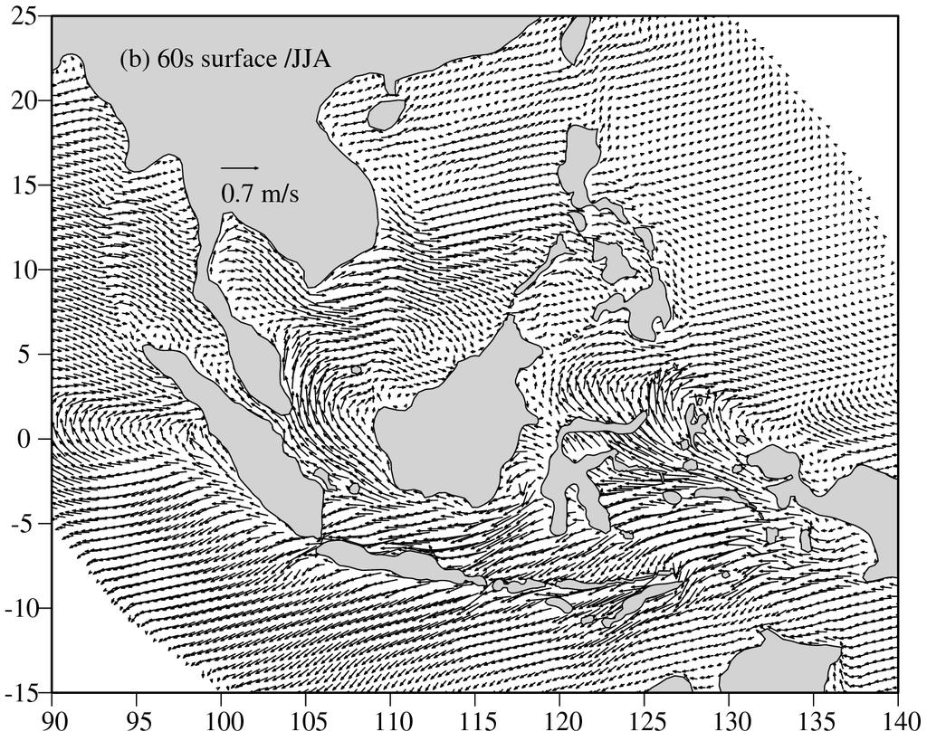
51

52 Figure 4. Modeled seasonal mean current fields. a) 6s at surface in Winter (DJF). b) 6s at surface in Summer (JJA). c) difference of 9s-6s at surface in Winter (DJF). d) difference of 9s-6s in Summer (JJA). 51

53 Figure 5. Modeled seasonal mean current fields. a) 6s at 5m in Winter (DJF). b) 6s at 991 5m in Summer (JJA). 52

54 Figure 6. same as Figure 5 but at 1m 53

55 a) Luzon 6s c) Mindoro 6s e) Makassar 6s g) Lombok 6s i) Timor 6s -2-4 a) Luzon 6s 9s Luzon 9s J F M A M J J A S O N D Mindoro 9s -4-6 e) Makassar Makassar 9s J F M A M J J A S O N D g) Lombok Lombok 9s J F M A M J J A S O N D -3 c) Mindoro J F M A M J J A S O N D i) Timor Timor 9s J F M A M J J A S O N D b) -4 Karimata 6s d) -4 Sibutu 6s f) -8 Lifamatola 6s h) j) Ombai 6s b) Karimata -2-4 Karimata 9s J F M A M J J A S O N D Sibutu 9s Torres 6s Torres 9s f) Lifamatola 6s 9s -1 Lifamatola 9s J F M A M J J A S O N D h) Ombai 6s 9s -12 Ombai 9s J F M A M J J A S O N D.3 annual ave Summer(JJA) Winter(DJF).2.1 d) Sibutu 9s J F M A M J J A S O N D j) Torres 6s 9s 6s J F M A M J J A S O N D Figure 7. The annual mean, Summer (JJA) and Winter (DJF) mean transport (bar plot on the left panel) and the monthly variation of the volume transport (line plot on right panel) through a) Luzon strait, b) Karimata strait, c) Mindoro strait, d) Sibutu strait, e) Makassar strait, f) Lifamatola strait, g) Lombok strait, h) Ombai strait, i) Timor strait and j) Torres strait. In the bar plot (left panel), the first set bar is 6s and the second is 9s, the solid line empty bar is the annual averaged volume transport, the narrow red bar is the Summer (JJA) averaged and the wider blue bar is the Winter (DJF) averaged. In the line plot (right panel), the 6s volume transport monthly variation is represented by blue line with star marks and the 9s is represented by red line with circle marks. All Y axis with a unit of Sv ( x 1 6 m 3 /s). Negative/positive value represents Westward (Southward) / Eastward (Northward) transport. 54

56 17 18 C Figure 8. Decadal averaged temperature difference between 9s and 6s (9s-6s) of SODA reanalysis data. a) Winter (DJF) at surface, b) Summer (JJA) at surface, c) yearly averaged at surface, d) Winter (DJF) at 15m, e) Summer (JJA) at 15m, f) yearly averaged at 15m, g) Winter (DJF) at 5m, h) Summer (JJA) at 5m and i) yearly averaged at 5m

57 C 116 Figure 9. Same as Figure 8. but for modeled