Developments of the offshore wind turbine wake model Fuga

Transcription

1 Downloaded from orbit.dtu.dk on: Mar 06, 2018 Developments of the offshore wind turbine wake model Fuga Ott, Søren; Nielsen, Morten Publication date: 2014 Document Version Publisher's PDF, also known as Version of record Link back to DTU Orbit Citation (APA): Ott, S., & Nielsen, M. (2014). Developments of the offshore wind turbine wake model Fuga. DTU Wind Energy. (DTU Wind Energy E; No. 0046). General rights Copyright and moral rights for the publications made accessible in the public portal are retained by the authors and/or other copyright owners and it is a condition of accessing publications that users recognise and abide by the legal requirements associated with these rights. Users may download and print one copy of any publication from the public portal for the purpose of private study or research. You may not further distribute the material or use it for any profit-making activity or commercial gain You may freely distribute the URL identifying the publication in the public portal If you believe that this document breaches copyright please contact us providing details, and we will remove access to the work immediately and investigate your claim.

2 Developments of the offshore wind turbine wake model Fuga Department of Wind Energy E Report 2014 Søren Ott and Morten Nielsen DTU Wind Energy E-0046 January 2014

3 Abstract This is the final report of the project entitled Risø DTU Modelling Services carried out by DTU Wind Energy (formerly known as Risø National Laboratory) as part of the Carbon Trust s Offshore Wind Accelerator Stage 2 under a contract with Carbon Trust. The project is a follow up to a Carbon Trust s Offshore Wind Accelerator Stage 1 project called Linearized CFD Wake models. The earlier project resulted in the development, implementation and validation of the Fuga model. Fuga is a linearized CFD model that can predict wake effects for offshore wind farms. The main purpose of Stage 2 is to add more features to Fuga and turn it into a useful tool for offshore wind farm developers. The new features consist in Flexibility. Including the ability to cope with several types of turbines in the same project, thus making it possible to predict inter farm interactions. The graphical user interface has been greatly improved and a number of input/output facilities have been added. Stability effects. The effect of stability has been added through a modification of the eddy viscosity based on Monin Obukhov theory. The numerical solver developed in Stage 1 has been generalized in order to make it deal with the modified equations. Meandering. Meandering has been included in the form of a post processing of the model results that bend and twist the wake centreline. The meandering centrelines are calculated using a Gaussian process developed on the basis of measured spectra. An analysis of meteorological data from Horns Rev has been made in order to quantify the impact of non stationarity of the wind direction. The results are generalized so as to account for the uncertainties imposed by a ten minute mean value trend as well as by the distance between turbines and the met mast. The old model has been validated against a number of data sets. Some of these tests have been repeated in order to demonstrate and validate the new model features. Production data from Horns Rev 1 have been re analysed using well defined selection criteria for which the developed uncertainty models apply, and a comparison with data is made. Even if the model predictions fall within estimated error bars, the model seems to over predict the measured efficiencies by a few percent. The model works best for unstable, neutral and light stable conditions whereas the results for stable and very stable conditions are questionable. We suspect this is caused by a failure of the numerical solver that becomes progressively more severe as the stability increases. Approved by: Hans E. Jørgensen Checked by: Morten Nielsen In no event will the Technical University of Denmark (DTU) be liable for any damage, including any lost profits, lost savings, or other incidental or consequential damages arising out of the use or inability to use the results presented in this report, even if DTU has been advised of the possibility of such damage, or for any claim by any other party.

4 Contents 1 Introduction 5 2 Flexibility 6 3 Atmospheric stability modelling Theory Model equations Numerical methods 11 4 Wake meandering Data interpretation Turbulent scales Wake meandering modelling 19 5 Rotor averaging 23 6 Validation Repeats of old tests New Horns Rev 1 test 27 7 Guidelines Stability input to Fuga Roter averaging How to make a climatology with stability Fuga user interface 35 References 41 8 Appendix A: The Fuga help system 42 DTU Wind Energy E

5

6 1 Introduction This is the final report of the project entitled Risø DTU Modelling Services carried out by DTU Wind Energy (formerly known as Risø National Laboratory) as part of the Carbon Trust s Offshore Wind Accelerator Stage 2 under a contract with Carbon Trust. The project is a follow up to a Carbon Trust s Offshore Wind Accelerator Stage 1 project called Linearized CFD Wake models. The main outcome of this earlier project was the Fuga wake model, which is based on a linearized CFD model using the simple closure. The model is described in Ott (2011), the final report of the first stage of the project. 1. The present project aims at extending and refining Fuga and turn it into useful tool for the quantification of wake effects in wind farms and between wind farms. The report constitutes Deliverables 3 and 9 under Task 5 (cfr. Trust 2011). There are thus three purposes: 1. Technical documentation of added model features 2. Evaluation against measurements 3. User guidelines. The main objective of the present project is to make the Fuga model a more useful tool by adding some new features. The objectives fall into three categories: Flexibility. Stability effects. Meandering. Before describing the developments in more detail we briefly recapitulate the status of the old model. The old Fuga model (i.e. version 1.4) was validated as part of the Linearized CFD project in Carbon Trust s Offshore Wind Accelerator Stage 1, cfr. Ott (2011) and Ott et al. (2011). Actually three different versions of the model based on three different closures were evaluated. For each closure model predictions were compared to production data from Horns Rev 1, Nysted and Nibe wind farms. Gribben, de Villiers, Hui, Balcombe, Harrington, Peace, Mallins, Housley, Kristensen and Bech (2011) made a similar analysis of data from the North Hoyle wind farm. Furthermore, results from the simple version of the model were compared with wake deficits measurements taken at met masts located 2 and 6 km in the lee of Horns Rev 1. The following points summarize the results of the model: The simple closure was clearly better than the two other, more elaborate, and thus supposedly better, closures. Rather large discrepancies were found for data for narrow wind direction bins. This was partly explained by inaccurate wind direction data. The wind vane was out of order and one of the turbines was used as anemometer (inferring the wind direction from the yaw angle). Meandering was the second, more fundamental explanation. When data were collected in large enough wind direction bins, the effect of data being misplaced in the wrong bin becomes negligible, and the comparison becomes more benign towards the model. For relatively wide bins the comparison with data strongly favors the simple closure. In fact this version of the model leaves very little room for improvements. Model predictions (using the simple closure) of wake deficits show excellent agreement with data measured at the met mast M6, located 2km behind the last row, and M7, located 7km behind the last row. It should be noted that we have attempted to make the simplest possible (and still meaningful) adjustments of the model. 1 A publicly available version is found in Ott, Berg and Nielsen (2011) DTU Wind Energy E

7 2 Flexibility A certain lack of flexibility characterizes the old model. Most noticeable is the fact that it only works for one type of turbines at a time. This excludes calculations of farm to farm interactions unless they are assumed to be equipped with the same type of turbine. The new model is capable of working with WAsP project files. Thus WAsP is used to define turbine types and locations and the workspace generated by WAsP is used as input to Fuga. One implication of this is that the turbines can be split into groups (and even sub group) each with their own turbine type. Another implication is that a different wind climate can be assigned to the individual turbines or to turbine groups. In this way the model can take spatial variations of the wind climate into account. Fuga handles this by making a separate calculation for each wind climate to produce the results the turbines associated with it. Thus Fuga still only uses one wind climate at a time to calculate wake effects. This is permissible because the largest wake effects are due to neighbouring turbines. The old model only used the velocity at the hub height plane to estimate the thrust assuming that the trust scales with U 2 (z hub ), the free stream velocity at hub height. With several turbine types the flow field has to be calculated at several different heights, and the availability of the whole 3D flow field can be used also to make a (supposedly) more accurate estimate of the thrust by replacing U 2 (z hub ) with a numerical averaging of U 2 over the rotor plane. These changes have resulted in a major revision of data structure and functionality of the graphical user interface. Numerous changes have been made to expand and improve the functionality of the graphical user interface (GUI). The built in help system documenting the changes that were made is included as Appendix A. 6 DTU Wind Energy E-0046

8 3 Atmospheric stability modelling The old model did not incorporate effects of stability. In the verification data were not split up according to stability, hence the comparison could be misleading, and it would perhaps have been better to pick only near neutral data. However, the inclusion of stable and unstable data may not actually make much difference in terms of predictions of net annual energy production. Long range, farm to farm interactions could, on the other hand, depend more strongly on stability. The new model is based on the simple closure, but with a stability dependent eddy viscosity as explained below. 3.1 Theory In the new model atmospheric stability is represented as a change of the eddy viscosity profile of the approach flow. The eddy viscosity K determines the velocity profile through the relation K(z) du dz = u2 (1) Following the simple philosophy we assume that the eddy viscosity is unaffected by the presence of a wake. Measurements in wakes show increased levels of turbulence, but the length scale is decreased at the same time so that the effect on K seems to be limited. The buoyancy term in the momentum equation is ignored. This eliminates the need for a (potential) temperature equation. A temperature equation coupled with the momentum equation via a buoyancy term would produce solutions that exhibit gravity waves. It is likely that gravity waves can have interesting effects under very stable conditions, e.g. when the turbines excite standing waves in the farm. This has been observed in the lee of islands with a small mountains on them, where it causes the wind to speed up instead of slow down. It would not have been very difficult to include such buoyancy effects, but since they are not likely to be of much importance, except perhaps for some very rare cases, we choose to keep things as simple as possible and neglect the coupling via buoyancy. Buoyancy is therefore only modelled indirectly through the eddy viscosity K. In the old model the eddy viscosity, K, was set equal to κu z, which is its value in a flat, homogeneous terrain (such as an open sea) under neutral, barotropic conditions. For non neutral conditions we will use the eddy viscosity dictated by Monin Obukhov (M O) similiarity theory, Monin and Obukhov (1954) (see also Monin and Yaglom 1975). M O theory introduces the Monin Obukhov length scale L defined as T u3 L = κg wθ = T u2 (2) κgθ where T is the absolute temperature at the surface, u = w u is the friction velocity, g is the acceleration of gravity and θ is the potential temperature and θ = wθ /u. L/u is a corresponding time scale and θ is a temperature scale. When these scales are used to write the equations in non dimensional form a small miracle happens: the equations are the same no matter what L is! It should be noted that the equations are the Navier-Stokes equations in the Boussinesq buoyancy approximation and without the Coriolis force. The use of the eddy viscosity concept is sometimes also called the Bousinnesq approximation, but that assumption is not necessary to derive the theory, nor do we need to postulate any closure. We are, in other words, talking about equations that have fully realistic turbulent solutions. In flat terrain it gets even better because the boundary conditions for the mean fields become independent of L too. As a result the mean velocity profile must have the form U(z) = u (f(z/l) f(z 0 /L)) (3) where f is a universal function that can be determined from measurements. It turns out DTU Wind Energy E

9 that f(ζ) has logarithmic pole at ζ = 0 so that it can be written as f(ζ) = 1 κ (log ζ ψ m(ζ)) (4) where ψ m is more well behaved. The constant in front is the inverse von Karman constant. Using ψ (3) becomes U(z) = u κ (log z/z 0 ψ(z/l) + ψ(z 0 /L)) (5) This is Monin Obukhov similiarity theory in a nutshell. If we assume that there is such a thing as an eddy viscosity then (1) yields K = u κz (6) φ m (z/l) where The mean potential temperature profile has a similar form 2 φ m (ζ) = 1 ζ ψ m(ζ) (7) θ(z) = T + θ κ θ (log z/z 0 ψ h (z/l) + ψ h (z 0 /L)) (8) There is a simple relation between temperature and potential temperature: θ(z) = T (z) + g/c p z (9) where T (z) is the absolute temperature at height z and C p is the specific heat of air at constant pressure. In M O theory stability varies with height. Near the ground the profiles are dominated by logarithm and close to neutral while the ψ functions become more an more important as the non dimensional height ζ z/l increases. In this respect M O theory differs from the once very popular Pasquill (1974) stability class system, where stability is independent of height. For wind turbines z hub /L would be a relevant stability measure, but since the hub height does no vary very much for offshore turbines we follow Gryning, Batchvarova, Brummer, Jørgensen and Larsen (2007) and use 1/L to define stability classes (see table 2 in this report). In the new mode the look up tables have three entries: kz 0, β and ζ 0 z 0 /L. The old model had only two (kz 0 and β, see Ott et al. 2011). The extra dimension of the tables make them considerably more voluminous. M O theory assumes equilibrium with constant fluxes that do not vary with height. For offshore wind farms there could be a problem because non neutral situations often corresponds to situations that are created by a temperature difference between sea and land. If the wind blows from land to sea and the land is warmer than the sea then the sea will cool the air and create a stable layer with a capping inversion that grows very slowly with the distance from shore (the fetch). While the stable layer cools it approaches a neutral layer, and the assumption of equilibrium could be violated. Lange, Larsen, Højstrup and Barthelmie (2004) argue that this seems to be the case for the Nysted wind farm. Cold air on a warm sea will of course create an unstable layer that also decays to a neutral layer. The stability over open sea thus tends to be neutral, although sea temperature differences over long distances can make stability deviate from neutral and radiative cooling from clouds can create convection. Sathe, Gryning and Peña (2011) analysed met data from Horns Rev and found that unstable conditions are much more common for NW winds than for SW and explains it as caused by the general N S gradient of the sea temperature. Stability generated in this way should be similar to stability over a land surface, whereas stability generated by temperature differences between land and sea is probably more complex. A further investigation of this is needed, but this falls outside the scope of the present project. 2 ψ h (z 0 /L) is usually small and the term is often neglected. 8 DTU Wind Energy E-0046

10 Theory says that ψ m and ψ h are universal functions of ζ in the equilibrium surface layer under perfect, barotropic conditions. In practice these requirements are only met approximately and plots of ψ = Uκ/u log(z/z 0 ) against z/l always a great deal of scatter. There are therefore many different bids on what the ψ functions should look like. It is conventional to use the functional form φ(ζ) = (1 + a ζ) n (10) with two different sets of constants a and n for ζ > 0 (stable) and ζ < 0 (unstable). With two ψ functions we end up with 4 sets of constants. We have chosen the following functions which are consistent with the data analysis of Högström (1988): φ m (ζ) = { ( ζ) for ζ > 0 ( ζ) 0.25 for ζ < 0 (11) φ h (ζ) = { ( ζ) for ζ > 0 (1 12 ζ) 0.5 for ζ < 0 The uncertainty of these profiles is considerable, especially for strong stability where not much is known for values of z/l larger than about 1. We are therefore in trouble when z hub > L > 0. Very stable conditions with L less than about 100m are therefore out of Fuga s reach. It should be noted that the boundary layer depth generally decreases with L and for extreme stability the boundary layer may not even reach up to the turbine rotors, and the surface layer will be even more shallow. In such situations the shape of the wind profile will depend on many factors such as the sea land effects mentioned above, effects of baroclinity, the presence of a low level jet etc. It therefore becomes more and more impossible to maintain the assumption of a universal and predictable behaviour as stability increases. The fluxes of momentum and heat that go into the definition of L can be measured directly with a sonic anemometer. In case sonic anemometer data are not available L can be estimated from wind and temperature profiles. Over a sea surface stability is driven by the air to water temperature difference. It is therefore important to have measurements of temperature in the water as well as in the air. In principle two air temperatures taken at different heights could also work, but the difference is so small that it easily becomes very inaccurate. It is therefore essential that offshore met masts include water temperature measurements. L can be estimated from ten minutes values of air and water temperatures, a wind speed, current and an estimate of the surface roughness. We will assume that the current is negligible and obtain the surface roughness from Charnock s (1955) relation: (12) z 0 = A c u 2 /g + B c ν u (13) where A c is the Charnock constant (following Peña and Gryning (2008) we use A c = 0.012), ν is the molecular viscosity, and B c = 0.12, Grachev and Fairall (1996). A second term has been added in order to accounts for the limit of laminar flow at very low wind speeds. Using M O profiles we then have enough equations to determine L. In general the equations must be solved numerically, but for near neutral conditions there are simplifications. From observations of wind speed U taken at height z u, air temperature t a taken at height z t and sea surface temperature t s we can form a so called bulk Richardson number R b : R b = gz ref(θ(z t ) T s ) T s U 2 (14) where z ref is a reference height of our choice - its only purpose is to make R b non dimensional. Inserting profile functions into (48) we find the following relation z ref /L = R b (log z u /z 0 ψ m (z u /L)) 2 log z t /z 0 ψ h (z t /L) For near neutral conditions we have z t /L z u /L 0 so that we are allowing us to drop ψ m and ψ h. Using a good guess for the surface roughness, say z0 = 0.1 mm, we then arrive at DTU Wind Energy E (15)

11 the estimate 1 L R b z ref (log z u /z 0 ) 2 log z t /z 0 (16) This relation does not require any knowledge of the universal functions. Evaluating R b from data is straight forward and (16) gives good estimates for z/l < 0.1. Thus equation (16) suggests an approximate relation between z ref /L and R b even if an exact relation does not exist within M O theory. Grachev and Fairall (1996) derived such an empirical relation, which is widely used. However, it is only valid for the special case z ref = z u = z t = 10meter, and it is not obvious how to generalize it to other heights. Consequently many different methods are in use. In order to put an end to this confusion we have made a tool called AMOK that solves the equations numerically and yields L from t s, t a and U measures at any heights. The numerical solution starts with (16) to obtain a first guess on 1/L. This is then used to evaluate ψ m and ψ h so that U and θ can be evaluated from (5) and (8) and z 0 is calculated from (13). The next iteration is the same except that it starts with (48) rather than 16. The scheme is very robust and seems always to converge to a solution provided one exists. It converges rather slowly, however, and an alternative scheme is used to converge down to machine precision. The second scheme is a 2D Newton-Ralphson iteration for the two variables U and θ with z 0 eliminated by means of (13). The combined scheme is fairly robust and efficient except for rare cases with a combinations of extremely stable conditions, low wind speed and large difference of z u and z t. In the data studied so far cases with no solution are extremely rare, and only occur below the cut in speed for most wind turbines. 3.2 Model equations The governing equations are basically the same as was used in Ott et al. (2011) for the simple closure. They are formulated in a mixed spectral setting, where the wind field (u, v, w) and the pressure p have been Fourier transformed along the two horizontal directions x and y. The fields are therefore functions of two wave numbers k 1 k 2 and z. The equations read u 0 ik 1 u 1 + w 1 u0 z ik 1 u 1 + ik 2 v 1 + w1 z = k 2 K u 1 + z K u1 z + K z ik 1 w 1 ik 1 p 1 + f 1 1 (17) u 0 ik 1 v 1 = k 2 K v 1 + z K v1 z + K z ik 2 w 1 ik 2 p 1 (18) u 0 ik 1 w 1 = k 2 K w 1 + z K w1 z + K z w 1 z p1 z (19) = 0 (20) where k 2 = k 2 1 +k 2 2. The difference is that K now depends on stability as described in section 3.1. The boundary conditions are: u(k 1, k 2, z 0 ) = 0 v(k 1, k 2, z 0 ) = 0 w(k 1, k 2, z 0 ) = 0 u(k 1, k 2, z i ) = u 0 (z i ) v(k 1, k 2, z i ) = 0 w(k 1, k 2, z i ) = 0 (21) 10 DTU Wind Energy E-0046

12 3.3 Numerical methods The friction velocity is eliminated from the equations by scaling the velocity components u, and pressure and rotor forcing with u 2 as described in Ott (2011). In the mixed spectral formulation there is only one independent variable, z, since k 1 = k cos β and k 2 = k sin β merely act as constants. Using the variable kz instead of z eliminates k, but we still have β, and kz 0 from the boundary conditions (and from u 0 ). We also have ζ which we write as ζ = z L = kz(z 0/L) kz 0 = kζ 0 kz 0 (22) where we have defined ζ 0 = z 0 (23) L In the old model the look up tables had two entries: kz 0 and β. Now we have three: kz 0, β and ζ 0 The solution method described in Ott et al. (2011) was applied with a modification that takes the changed definition of K into account. In the original procedure the variable z was replaced with the variable t = log z/z 0 in the lowest part up to kz = 1, while s = kz was used in the upper layer. In the new model we generalize the definition to t = log z/z 0 ψ(z/l) + ψ(z 0 /L) = log s/kz 0 ψ(s/kz 0 ζ 0 ) + ψ(ζ 0 ) (24) We are, in other words, essentially using the unperturbed velocity to indicate the height above the ground. The second identity show that t can be expressed in terms of s and the two parameters kz 0 and ζ 0. The following identity can be used to change the equations to the new variable t = K κu z The numerical solution to the linearized equations is the Achilles heel of the model. It was only with great difficulty we managed to solve the equations for the neutral case, and from start there was no guarantee that it would work for all stabilities. The problem is that the equations have particular solutions that increase or decrease extremely fast, and finding the well behaved linear combination that solves the problem is like finding a needle in a haystack. The problem becomes less severe when K is large. This happens on the unstable side which is therefore quite benign. On the stable side, however, K gets smaller and smaller as the stability increases. It was therefore expected that the numerical solution would break down at some point, but hopefully only at very strong and rare stabilities. The first expectation came true, but unfortunately the solutions seem to misbehave even at quite moderate stabilities. It was not the intention to develop new numerical solution methods in the present project, but a few ideas were tried none of which lead to an improvement. This problem is something that needs to be looked at in the future. (25) DTU Wind Energy E

13 4 Wake meandering 4.1 Data interpretation Before we proceed to the description of the wake meandering model, we need to discuss the interpretation of meteorological data in terms of input to flow models. Real world 4D fields Weather Predictions Measurements Met mast SCADA Model world Idealized flow Homogeneous Stationary The diagram illustrates the various ingredients that go into the validation of a wake model. We have the real world with its complex fields (velocity, temperature etc.) and complicated interactions. We don t have full access to the real world, but have to be make do with measurements such as met mast data and SCADA data. These are essentially point measurements and we have to make some kind of interpretation in order to fill the gaps and create an idealized model world which our wake model can work with. In the model world the fields have to be statistically stationary because otherwise we cannot make a Reynolds decomposition and therefore we cannot apply a RANS model. Horizontal homogeneity is also a necessary assumption in our case. Once we have decided how to interpret the data we can make model predictions which finally can compared to data. Strictly speaking, you cannot be compare directly to the real world which remains a bit on the sideline in the diagram. If the comparison is good there are two possibilities: either the data interpretation and the model are both correct or they are both wrong. Two wrongs can make a right, and this may if fact occur if the data interpretation is incorrect and the model is tuned to make a good comparison. It is therefore necessary to discuss data interpretation. In order to do this in a simple way we will make two different interpretations and work out the consequences for the data comparison. We will also focus on the wind direction because wake effects are very sensitive to this parameter. Similar considerations can be given to other parameters such as wind speed and stability measures, but the wind direction has the largest impact. The traditional interpretation of met data is to regard each ten minutes period as belonging to a statistically stationary time series with (abstract) mean values equal to the corresponding ten minutes averages. In figure 1 this corresponds to the black, piecewise constant curve. The implication is that a single mean value of the wind direction is assigned 12 DTU Wind Energy E-0046

14 Figure 1. Green: wind direction time series. Black: mean value, traditional interpretation. Red: mean value, alternative interpretation. every ten minutes and used as input to the model. This of course does not make the average wind direction equal to the true mean wind. We could shift the ten minutes periods by e few minutes and get different mean values with the same data. We will therefore investigate the implications of making a more realistic, alternative interpretation. The alternative interpretation is illustrated by the red curve. Here the mean value is changing continuously in time in a piecewise linear manner connecting the ten minutes averages. This mean that each ten minutes period corresponds to a range of mean values depending on the slopes of the linear pieces. Instead of feeding the model with one wind direction for each period, we should feed the model with a range of values distributed around the observed average value. In other words, we are still treating the model world flow as statistically stationary, but allow more variation of the wind direction input than in the traditional approach. Figure 2 shows a histogram of measurements of θ, the difference between consecutive ten minutes averaged of the wind direction. The red dots show a fit to an exponential distribution: P θ (x) = β/2 e β x (26) Further data analysis has shown that the parameter β depends on both wind speed and stability, and the following expression has been fitted; β = a 1ζ 0 + b 1 u (27) 1 + a 2 ζ 0 + b 2 u The values of the fitting constants are listed in Table 1. These values are default values in Fuga. They could be used tentatively for other locations than Horns Rev, even if site specific values based on local measurements are to be preferred. Table 1. Constants to be used in (27). Stability a 1 [-] a 2 [-] b 1 [s/m] b 2 [s/m] Stable Unstable We need the distribution P δθ of the variable δθ θ θ where θ is the wind directions to be used as model input and θ is the observed ten minutes average wind direction. In figure 1 δθ represents the difference between the red line and the black line. Each linear piece of the red line corresponds to an interval of mean values with θ /2 < δθ < θ /2 (28) Thus all the flow cases corresponding to the column around θ in the histogram in figure 2 should be distributed evenly on this interval. In terms of probability this can be expressed as DTU Wind Energy E

15 fhdql Figure 2. Histogram of θ, the difference between successive ten minutes averaged of the wind direction. Data were from met mast M7 located to the east of Horns Rev 1. The red dots is a fit to an exponential distribution. P θ ( θ) d θ for θ /2 < δθ < θ /2 θ dp δθ (δθ) = 0 otherwise (29) Integrating this we find P δθ (x) = 2 x where we have used (26) and P θ (x ) x dx P + θ (x ) 2 x x dx = β Γ(0, 2β x ) (30) Γ(k, x) = x t k 1 e t dt (31) is the incomplete gamma function. The way to apply the alternative interpretation is to convolute the distribution of observed average directions (which could be a rectangular distribution on a bin) with P δθ. This is best done in the Fourier domain, where it is just a matter of multiplying with a filter φ δθ given by φ δθ (k) = P δθ (x) e ikx dx = 2β k Arctan k 2β The width of the filter P δθ, determined as the square root of the second central moment, is equal to 1/(β 3). Figure 3 shows results from a wake model test made in the EERA-DTOC project. The graphs show normalized power deficits in the crosswind rows of Horns Rev 1 for Fuga and 7 other wake model. A narrow, 5 degree wide, wind direction bin centrered around a wind direction that runs parallel with the turbine rows has been chosen. For the narrow bib all the models predict larger deficits than was measured. This test is based on the conventional data interpretation. The red curve is the Fuga results when we use the alternative representation. For historical reasons a 5 degree wide square filter was used instead of (30). The width based on the second central moment is therefore 5/ 12 degrees. Equating this to 1/( 3β) we get β = 0.40 which is exactly what (27) assuming neutral conditions and U=8m/s. The improvement of the comparison with data using the alternative interpretaion is quite evidently. It is worth noting that the interpretation does nothing to the model itself, it is only the way model results are binned before comparison with data which is affected. The same kind of tests were made by Barthelmie, Hansen, Frandsen, Rathmann, Schepers, Schlecz, Philips, Rados, Zervos, Politis and Chaviaropoulos (2009) in the UpWind project (32) 14 DTU Wind Energy E-0046

16 where bins as narrow as ±1 degree were used. The intension is to test the ability of wake models to handle multiple wakes (wakes in wakes), but it is not possible to determine the cause of the wake deficits being larger than observed. It could be caused by the models wakes being too narrow or too strong or it could be caused by the wind direction being uncertain. The present analysis does not solve this dilemma, but it shows that the uncertainty of the wind direction should not be neglected. Using this kind of test for model tuning is therefore highly problematic. Data issues and problems with establishing flow cases has been discussed before. Barthelmie et al. (2009) list a number of issues, but largely see it as problems that the models should be able to deal with. Here we see it more as a measurement issue, which can be dealt with by further analysis of met data, preferably from the site in question. Fuga + 5deg filter Technical University of Denmark Figure 3. A slide showing wake model results averaged over a narrow wind direction bin. The stationarity analysis can be extended to include effect of inhomogeneity in a simple way. The wind direction measured on a met mast is likely to differ from the wind direction at a turbine placed far away from it. If the met mast is located directly upwind with respect to the turbine, there will be a delay X/U before the air that pass by the mast will pass by the turbine. By Taylor s hypothesis we assume that the wind field is frozen and just slides downwind with velocity U without changing. This assumption is of course not perfect, but it is correct in an average sense. Vincent, Larsén, Larsen and Srensen (2013) investigated the correlation between wind speed measurements taken at a pair of offshore met masts and the spatial and temporal decay of the correlation. This study confirms that the signals are best correlated when a time delay equal to the travel time X/U is applied. It also shows that only the low frequency parts of the signals are correlated and that the decay the Fourier component corresponding to frequency f goes like e af X /U, where a is a constant that depends on the angle between the wind direction and the line connecting the two masts (or mast and turbine). In the downwind case a = 4.1 while a = 7.7 in the crosswind case. Travel DTU Wind Energy E

17 times of several minutes are common in offshore wind farms and hence eddies corresponding to time scales 4 to 8 times longer than the travel time will be correlated. These eddies are found in the second group marked drift in figure 6. We therefore assume that the trend in the ten minutes average wind direction persists during the travel from the mast to the turbine. In other words, we simply extrapolate the red segment in figure 1 by the delay in order to predict the most likely behaviour at the turbine. The corresponding segment is illustrated as the blue segment in figure 4. Finally we assume that this procedure can be followed even in situations where the turbine is not directly downwind of the mast. It is a crude model, but it should give some of the right tendencies. Figure 4. The blue line corresponds to the assumed wind direction interval seen at distance X from the mast. In terms of math we simply replace (29) by P θ ( θ) d θ for ( t T ( 2) 1 θ < δθ < θ ) t T θ dp δθ (δθ) = 0 otherwise where t = X/U and T is the averaging time (e.g. ten minutes). Inserting (26) into (33) and integrating yields P δθ (x) = β 2 β 2 { } 2β x Γ(0, 2t/T +1 ) + Γ(0, 2β x 1 2t/T ) { } 2β x Γ(0, 2t/T +1 ) Γ(0, 2β x 2t/T 1 ) for t < T/2 for t > T/2 Again the Fourier transform is relatively simple: φ δθ (k) = P δθ (x) e ikx dx = β ( ) k(1 + 2t/T ) k(1 2t/T ) Arctan + Arctan k 2β 2β Figure 5 shows how a 5 degree wide bin with observed average wind directions at M7 translates to a wider distribution of observations at M6. The red line is the model, the convolution of (34) with a 5 degree wide rectangular filter. The observed distribution is a bit wider than the model distribution, but it is not completely far out. This could perhaps be expected since we did not take decay of eddies into account. 4.2 Turbulent scales Before we describe the meandering model we need to elaborate on the various time and length scales that are involved and explain in more detail the assumptions that have been made about the physical processes that govern the wake behaviour. Figure 6 shows an old spectrum taken from Courtney and Troen (1990), where we have identified five different regimes. The spectrum is made from one full year of wind data and thus covers a wide range of time scales. Note that areas below the graph are proportional to the corresponding turbulent 16 DTU Wind Energy E-0046 (33) (34) (35)

18 Figure 5. Green line: pdf of average wind directions observed at M7 with bin centre shifted to zero. Dots: pdf of the corresponding average wind direction observed at M6. Red line: model prediction of the pdf at M7. kinetic energy. The high peak at around 10 6 Hz is due to diurnal variations and is part of a big mountain of low frequencies. Although these slow fluctuations represent almost all the kinetic energy, they effectively just determine the mean wind speed and direction in any given ten minutes period, and we would not normally refer to this as turbulence. At slightly higher frequencies we have the fluctuations that can make the wind direction change over 10 minutes, which were discussed and analysed in section 4.1. These variations are caused mainly by mesoscale mechanisms such as the passage of weather systems, convection cells, gravity waves or clouds. Near the surface this mainly affects horizontal motion are mainly horizontal even if the flow as such is not two dimensional. Lindborg (1999) analysed long range spatial velocity correlation data derived from airplane flights and saw two ranges. For low wave numbers k < 2π/500km) the spectrum varies as k 3 which is due to an enstrophy cascade that represents true 2D behaviour. For larger k in the range 2π/30km 2π/500km the spectrum varies as k 5/3, which could in principle be caused by a 2D energy cascade, but Lindborg argues against this and prefers to interpret it as 3D behaviour caused e.g. by gravity waves which can also produce such a range. When in figure 6 the local maximum at 10 2 Hz is taken to divide 2D from 3D behaviour, the 2D should be taken with a grain of salt. Even if the motion is mainly horizontal the flow a mixture between 2D and 3D behaviour. The next blob marked meandering represents motion that takes place on top of the drifting mean wind. In figure 1 it is contained in the excursion of the green curve from the red curves. These scales are responsible for the distortions of the wake centrelines that are referred to as meandering. We could characterize the meandering eddies as large enough to move a cross section of the wake as a whole, yet small enough the make the centreline wiggly waggly. Still smaller scales (larger frequencies) represent 3D eddies that are comparable in size with the wake cross section but too small to contain it. This regime is marked scrambling because it represents eddies that make a lot of mess by moving around parts of the wake. Modelling the effects of this is, to say the least, not straight forward, and today it can only really be done with large eddy simulations. Finally, we have the eddies that are much smaller than the wake cross section. They only stir the wake locally and cause momentum to spread in diffusive manner. In this way they tend to smooth out the mess created by the slightly larger eddies, but they never really succeed in doing so. It is only the effect of the smallest eddies that can truly be represented by an eddy viscosity. The main features of the spectrum shown in figure 6 are common to datasets from mid latitudes. The Australian dataset studied by Ayotte, Davy and Coppin (2001) shows similar trends. In general the high frequency, 3D part is more site specific than the low frequency 2D part. The 3D turbulence is mainly created by surface friction and the turbulent kinetic energy is proportional to u 2. The level therefore depends on the the wind speed (at 10m, say), but also on terrain since u increases with increasing roughness (for a fixed U). Therefore DTU Wind Energy E

19 imes 2D 3D n 2011 enmark Courtney & Troen 1990 Figure 6. Spectral regimes - see text for an explanation. The spectrum is from Courtney & Troen (1990). there is generally more turbulence in this part of the spectrum for onshore sites than for offshore sites. Larsén, Vincent and Larsen (2012) found that the low frequency mesoscale part, is very similar from site to site, even from onshore to offshore sites. Moreover, the low frequency part of the spectrum does not seem to depend on stability nor on the average wind speed. This makes sense if we think of phenomena such gravity waves, clouds or convection cells which can be transported around by the main wind without being dynamically coupled to it. Eddy viscosity can only truly represent the smallest eddies, but for a realistic RANS model the eddy viscosity must represent a larger part of the turbulence. It could be argued that the result of the action of scrambling eddies work a bit like viscose diffusion when a time averaging is applied. As we go to larger scales, the eddy viscosity becomes less and less realistic and we can ask ourselves whether we should consider the larger scales as described by the model. If we go to the limit and include all scales, we end up with a model describing something like one year averaged wakes. Depending on the wind rose, the wakes would spread out from the turbines in all directions and the model would not be able to handle shadow effects at all. We are therefore forced to exclude too large eddies from the model world. This means that we can only predict what would happen if the large eddies were not there. Comparison with data from the real world then becomes complicated by the fact that large eddies do exist in the real world. It is also difficult to say exactly where we should draw the line between large and small eddies. We could perhaps answer such questions if we 18 DTU Wind Energy E-0046

20 had a stringent derivation of the model equations from first principles, and if we had a deep understanding of the interactions between different scales of turbulence. But unfortunately we are very far from such an understanding. We therefore have to make interpretations and guesses when we relate model results to the real world. The Fuga model is based on the following interpretation of the situation. We will assume that eddy viscosity is able to describe the effects of the smallest and the scrambling, eddies, but not the larger ones. The main reason is that a RANS model does not know about large eddies, unless the explicit mechanisms that create them are included in the model. Thus if gravity waves create meandering eddies, the model should be able to deal with gravity waves before we can assume that these eddies are incorporated in the model results. A time resolved model would be needed for that, and RANS models are not (should not be) time resolved. It would take an extremely complex model to reproduce weather on large scale and the local effects if it on small scales, but in principle this can be done by nesting models of progressively finer resolution. The demands for computing power for such a model would be exorbitant. The finest level would probably have to be a LES model, and the next level should be sophisticated enough to provide realistic boundary conditions for the LES model that can reflect the effect of mesoscale eddies. A LES model alone is not enough because it only transforms boundary conditions to bulk behaviour. In other words, even if the LES model exhibit a great deal of physical realism, the results are no better than the eddies we feed to it. We are looking for a much simpler solution. In our case we use the simplest possible RANS model which certainly does not include any mesoscale behaviour, and consequently we interpret the model results as representing the behaviour of wakes in an idealized world where mesoscale eddies do not exist. They do exist in the real world, but, to the extend it makes sense, our interpretation allows us to add mesoscale effects as a kind of post processing, and we can add them without double counting. We should of course make sure that the CFD model was not tuned to reproduce data that include mesoscale effects, but that is not the case for the simple closure we use because it does not have any adjustable parameters. 4.3 Wake meandering modelling So far we have argued that meandering is an aspect of real wake behaviour that present day models cannot cope with in a fully realistic manner. The old model is no exception. In the new model meandering is to a large degree put in by hand as a simple post processing of model results. In section 4.1 we discussed the effect of slow variations of the wind direction and showed how this and the effect of distance to the met mast could be treated by applying a appropriate filter. This takes care of the variations shown as the red line in figure 1. We still need to consider the meandering scales in figure 4.2 which are represented by the difference between the green and the red lines in figure 1. The following analysis is based on wind data from sonic anemometers sampled at 20Hz. The data was divided onto ten minutes long time series each of which were de trended by subtracting a best fit straight line variation. Ideally the red lines in figure 1 should have been used for the detrending, but we have checked on a few examples that the two methods give the same results for all practical purposes. The original plan was to install the machinery of the DWM model ( Larsen, Madsen, Thomsen and Larsen 2008) into Fuga, but this proved more problematic than we had anticipated. In the DWM model wake trajectories are generated by following passive fluid particles in a simulated, frozen turbulent velocity field which is convected downwind with an appropriate, uniform velocity. In order to simplify things further, the downwind component is replaced by the constant advection speed, so that the fluid particle always stays within the same cross wind 2D slab of the frozen velocity field. The main problem is that the wake trajectories generated in this way stop meandering after a while. They look nice and wiggly waggly at the start, but eventually they all become straight lines. This does not happen right away, but only after a distance somewhat longer than the typical distance between the turbines. The DWM model is intended for estimation of wake effects from tur- DTU Wind Energy E

21 bines located immediately upwind at a relatively short distance, where the trajectories are still meandering. Used in this way the model results are not seriously affected, but when it is used for larger distances, comparable to the overall size of a wind farm, the spurious behaviour becomes a problem. The intention here was to model wake effects across wind farms and even between wind farms, and therefore something had to be done. The basic idea in the DWM model, and in Fuga, is that the momentum deficit in a wake can be treated as if it were a passive tracer. In other words, the wake behaviour is similar to a passive plume. In the near part of a wake, where the velocity in the wake centre is much reduced compared to the surroundings, this is a crude assumption. However, further downwind, where the wake is just a small perturbation, the assumption can be expected to hold. The justification for treating the wake as a passive tracer is therefore similar to the justification for the use of a linearised model, which we know works surprisingly well. We have found that the cause of the odd behaviour is that the 2D flow field in the slab containing the fluid particle is compressible. The simulated 3D flow is compressible so that v y + w z = u x For the 2D flow, where u is taken to be constant, the right side will act as a source term. In areas where it acts as a sink, the points where v = w = 0 will be attractors. The fluid particle in the 2D flow therefore stops moving when it hits an attractor. After having realized this, it was decided to use the full 3D incompressible flow to generate trajectories. This eliminates the problem. Meandering is implemented in the model using the kinematic simulation technique by Mann (1998). The kinematic simulation is based on rapid distortion theory (cfr. Mann 1994) which takes the effect of shear into account. The method has lately been modified by Peña, Gryning and Mann (2010) to incorporate modifications due to stability, and the modified model was validated against data from the Hovsore test station. The result is a machinery that can generate flow field examples which possess many of the statistical properties observed in real, atmospheric turbulence. (36) 0.6 fvhu*tl * Figure 7. Dots: normalized autocorrelation function of v obtained from simulated wind fields. Red line: fit. This simulation technique works well, but it uses much computer resources both in terms memory and cpu time. It is therefore usually run on a cluster. but Fuga is supposed to run 20 DTU Wind Energy E-0046

22 on a single PC, so something had to be done in order to speed things up. The cure was to approximate the trajectories with a Gaussian stochastic process, which is much easier to simulate - making a model of a model so to speak. The simulated trajectories are non Gaussian, even if the simulated fields are Gaussian, but a Gaussian approximation can reproduce the Lagrangian velocity autocorrelation function and therefore it will also get the second moment of the crosswind deviation of the trajectory right ( Taylor 1921). A large number of simulations were made for different stabilities (different values of 1/L) and velocity auto correlation functions were made separately for each of the two cross wind components. The simulated velocities were scaled with σ u. If time is replaced with the variable σ u t then σ u disappears from the problem and the autocorrelation functions can be expressed as v(t) v(t + τ) = σ 2 u f v (σ u τ) (37) w(t) w(t + τ) = σ 2 u f w (σ u τ) (38) where f w and f w depend on L but not on the wind speed. The functions behave similarly and a typical example is shown in figure 7. The uncertainty of f w is small for small time lags, and increases as the time lag increases. The tail would therefore probably have approached 0 in a nicer way if more simulations were used, and the undershooting (negative values) in this example is just noise. The red line is a fit of the form f v (s) = µ 2 (1 + λ s )e λ s (39) The expression fits all the data with values of µ and λ depending on stability. It is computationally inexpensive to generate a Gaussian process ˆv(s) with this autocorrelation function and obtain the deviation ŷ(s) = A formal solution that gives (39) can be written as where N is δ correlated Gaussian white noise, i.e 0 ˆv(s ) ds (40) ˆv(s) = 2µλ 3/2 s e λs N(s s ) ds (41) 0 N(s) N(s ) = δ(s s ) (42) Note that (43) is a solution to the equation ( λ + s) 2 ˆv(s) = 2µλ 3/2 N(s s ) (43) One can integrate this equation numerically or solve it using a Fourier transform (which transforms white noise into white noise), but there is an even faster method that generates ŷ(s) directly for a discrete set of s values. The simulation is therefore just a matter of putting some random numbers into analytical expressions. The derivation is rather lengthy and is therefore skipped. Some simplifications were made: ˆv and ŵ are taken to be independent and we do not include a û so that the fluid point moves downwind with constant velocity. This is convenient because the time delay before the wake from one turbine hits the rotor of another turbine is deterministic rather than stochastic. We are using the same constants for the spectra as is used in the DWM model. They are normalized with σ u because the experimental spectra were normalized in this way. For our purpose it would have been better if they were normalized with u, but σ u was preferred because it is much more robust to measure than u. According to Monin Obukhov theory σ u /u should be a function of ζ, but in reality it does not work. According to Panofsky and Dutton (1984) it is better expressed as a function of z i /L for the unstable cases, σ u /u 2.4 for neutral and moderately stable cases while for strong stability the value becomes quite large and unpredictable. Hicks (1981) presents experimental data and draws a curve that DTU Wind Energy E

23 indicates that σ u /u saturates at a value of 3.0 for very unstable conditions. However, this behaviour is not really supported by the scattered data. The value σ u /u = 2.4 for neutral conditions is, on the other hand, supported by a large number of experiments (see Panofsky and Dutton 1984), and because of the uncertainty for non neutral conditions we have chosen the value σ u /u 2.4 to account for all stabilities Figure 8. The µ parameter as function of the inverse Monin Obukhov length. Blue is for the v component and green is for the w component D Figure 9. The λ parameter as function of the inverse Monin Obukhov length. Blue is for the v component and green is for the w component 22 DTU Wind Energy E-0046

24 5 Rotor averaging Figure 10. The seven points used in the seven point method The thrust is usually evaluated from the simple formula T/ρ = 1/2 C T πr 2 U 2 hub (44) This is valid in a constant wind profile without shear. In blade element theory the thrust is calculated separately for blade elements using the local wind velocity. This indicates that we might (but see below) get a slightly better approximation if we integrate over the rotor disk: T/ρ = 1/2 C T U 2 da (45) disk The integral can be performed numerically to any desired accuracy, and Uhub 2 πr2 can be regarded as the first approximation: R 0 dr 2π 0 dθ F (r, θ) πr 2 F (0, 0) (46) A more accurate can be improved by using the following seven point method instead of a one point method: R 2π dr dθ F (r, θ) πr F (0, 0) F ( 2/3R, jπ/3) (47) The formula is valid if F is a polynomial in y = r cos θ and z = r sin θ with degree less than 5. It is most practical to arrange the seven points in three different heights: z hub and z hub ± 2/3R. The output from the model is restricted to certain levels that jump about 10% from level to level. An interpolation is made when evaluating U at the three desired heights, which spoils some of the accuracy, but the method is still definitely better than the one point method. Thrust curves are normally calculated assuming a logarithmic profile or measured indirectly by strain gauges placed on the tower. The thrust coefficient is then obtained using the DTU Wind Energy E j=0

25 one point approximation. When the seven point method is used the resulting effective hub height velocity tends to be larger than the actual hub height velocity, so that the estimated power production increases. In order to stay on the measured (or calculated) thrust curve, we therefore scale the results so that the seven point method gives the same results as the one point method for the free flow profile. In this way the production from an unobstructed turbine does not depend on which method is used. The rotor average velocity used for the thrust is also used for the production. Ideally we should come from the rotor average of U 3, but the error introduced is negligible. The seven point method is optional in the Fuga GUI. It should be noted, however, that (45) we cannot simply use the C T values from an official thrust curve unless the blades are individually pitch controlled. When the blades do not have individual control, the angle of attack will change as a result of the shear as the blade completed a circle. When the turbine operates below rated power, the angle of attack is optimized and any change from the optimum value will decrease the performance. In that situation an increase of the wind speed will in fact result in a decrease thrust and a decrease of production. Therefore it is likely that the overall performance drops because of shear rather than increases. We therefore emphasize that the seven point method should not be used for turbines without individual pitch control. 24 DTU Wind Energy E-0046

26 6 Validation Model evaluation addresses the question of justifying the correctness of a model. This could be divided into three aspects: 1. Model tuning. Empirical basis for simplifications including justification of model constants. 2. Model validation. Comparison of model predictions with measured data (different from those used for 1). 3. Code verification. Checks that can justify that computer code is performing the tasks it is supposed to do and that this is actually leading to a proper solution of the problem. This report mainly describes how we will deal with model tuning and model performance. In this project code verification has been informal consisting in various cross checks that can be made along the way as the programs were developed. This can involve comparison with known, analytical solutions to special or limiting cases, the making of a mirror program on a different platform (e.g. Mathematica) and debugging in general. By now Fuga has into a complex application as more and more features have been added, and the resources necessary for debugging have been much larger than anticipated. In this section we compare model results with experimental data. The original plan was that Carbon Trust should provide test data, but no data was delivered. It is our impression that various Carbon Trust partners have tested the model against data from a number of offshore wind farms, but the results of these tests have not been shared with us. The validation is therefore less complete than it could have been. 6.1 Repeats of old tests The old model has been successfully validated against data from several offshore wind farms and the new model was run for the same cases. As for the old model neutral stability was assumed even if data was not necessarily sorted by stability. The new model generally reproduces the results of the old model. Due to changes of numerical procedures the results are not exactly the same. Figure 11 show a repetition of the validation against Horns Rev 1 production data using the new model. No filters were applied and the same input were used as to the old model: U = 10m/s, ζ 0 = 0 and z 0 = 0.1mm. The same qualitative behaviour is seen with an under prediction of the efficiency for the narrowest bin. For the wider bins there is an excellent agreement between the old model and data while the new model over predicts a few percent for the higher row numbers. In figure 11c both meandering, trend and spatial filters are included. This clearly improves the agreement with data, especially for the narrow ±2.5 degree bin, where the raw results vastly under predict the data. This changes when meandering and the filters are applied. Of these the spatial de correlation filter has the largest impact. The results change from under prediction to a slight over prediction. This could be caused by the way data were screened. The data represent ten minute periods where the averages of the preceding period fall into the same wind speed and direction bins. The idea was to select as clean cases as possible, but even if the screening might have some of that effect, the model results suggest that a large degree of uncertainty remain. A separate analysis of the met data to adjust to this particular screening procedure has not been made, but the result would have been a narrower filter that would bring model results and data closer together. DTU Wind Energy E

27 Normalized prod Fuga Fuga Fuga Data Data Data 0.50 a Row number Normalized prod Fuga Fuga Fuga Fuga Data Data Data Data 0.5 b Row number Normalized prod Fuga Fuga Fuga Fuga Data Data Data Data 0.5 c Row number Figure 11. Comparison of Fuga results with data from the Horns Rev I wind farm. U=10m/s, z 0 =0.1mm, a: the old model. b: new model without meandering or filter. c: new model with meandering and filter. 26 DTU Wind Energy E-0046

28 6.2 New Horns Rev 1 test Table 2. Stability classes used for the test and input used for the 9±1m/s bin. Description Class L interval 1/L 1 data z 0 ζ 0 Very unstable m< L <-50m -72m m Unstable m< L <-100m -137m m Near neutral unstable m< L <-200m -285m m Neutral 0 L >-500m -9257m m Near neutral stable 1 200m< L <500m 291m m Stable 2 50m< L <200m 88m m Very stable 3 10m< L <50m A new test was prepared for the Horns Rev 1 data set. AMOK was used to extract stability information from met mast M7 data together with SCADA data for turbine production. The wind direction was measured by a wind vane (z = 60m) and the velocity was measured by a cup anemometer (z = 70m) both on the met mast. M7 is located 6km to the east of the farm, which is further away from the farm than both M2 and M6, but the data from M7 are more reliable. Data was binned according to wind speed (2m/s bins), wind direction (5 degree bins) and inverse Monin Obukhov length binned in the classes defined in Gryning et al. (2007), see Table 2. The table also contains the bin averages used for model input. Data for U = 9 ± 1 m/s were selected for evaluation. The very stable cases were omitted. Only wind directions where the met mast was clear of the wake from the farm were used. Wind directions between N and NE are very rare, hence useable wind directions are limited to bins between 45 degrees and 240 degrees. Production data were selected for each turbine and data were rejected unless all upwind turbines were running. The average turbine production was therefore based on different data for each turbine since down wind turbines were allowed not be running. The production efficiency was calculated using the average production of all the running, unobstructed turbines as reference. For some wind direction bins there were little data or none at all. For an individual turbine the spread of the production data in a bin is about 30% 3. With between 10 add 100 realizations the error of the mean value is on the order of 3 10%. The error on the production efficiency is dominated by the estimate of the undisturbed production, which consists of an average over 8 18 turbines depending on the wind direction. The uncertainty of this average is lower that for a single turbine, but it is difficult to say how much lower because the productions from the individual turbines are correlated. There are also systematic errors such as spatial and temporal changes of wind speed and stability and coastal effects making the climate inhomogeneous. This suggests an accuracy of the data of perhaps 5%. The model was run for all the stability classes except class +3, where the criterion that z/l < 1 is violated. Three different settings were used: 1) raw results without meandering and filtering, 2) with meandering turned on and 3) with both meandering and trend and spatial filtering. The one point method was used in all cases. Figure 12 shows results for Class 0 (neutral). The effect of the stochastic meandering can be seen, but it is not large. This wold perhaps change if the measured σ u was used as input (the model uses the relation σ u /u = 2.4). The trend and spatial de correlation filter has more impact, perhaps a little bit too much in this case. The overall agreement with data is fair even if the model over predicts the efficiency by about 3%. Figure 13 shows results with both meandering and filtering for all stability classes (except very stable). The general picture is again that the model over predicts by 2 5%. Table 3 shows the mean value of the relative production for those wind direction bins where enough data exists to allow an estimate of the total production to be made. The 3 All percentages in this section are relative to the undisturbed reference production DTU Wind Energy E

29 model results and data in table 3 are therefore within the error bars and the discrepancy could therefore possibly be due to data uncertainty. However, the consequent over prediction could also very well be for real. The numbers cannot be compared between stability classes because the amount of available data differs slightly. In order to compare we have therefore also computed the predicted efficiency averaged over all directions for all seven stability classes. For class +3 (very stable) we have used L = 37m corresponding to ζ 0 = The value z hub /L 2 is beyond the range where the M O theory is valid, but we have tried to run the model anyway. Figure 14 shows the somewhat discouraging results. Something is happening in the stable (class +2) and very stable (class +3) the makes the efficiency increase with stability. We cannot prove it, but we believe that this odd behaviour is caused by the numerical problems that were mentioned in section 3.3. It should be noted, that these tests are not controlled experiments because we are testing two things at the same time. On the one hand we have the model of the uncertainty or imprecision of the measured mean values, and on the other hand we have the wake model. Discrepancies between model and data can likewise have more than one explanation. The width and depth of the dip of the efficiency around a direction where turbine columns are aligned with the wind, depend both on the predicted wake width and on the uncertainty we assigned to the wind direction measurement. If the dip is too narrow, say, then it could be because the model predicts a wake that is too narrow, but it could also be because we have underestimated the uncertainty of the wind direction. A more controlled experiment, where a discrepancy only has one explanation, should involve direct measurements of the wake. Table 3. Mean farm efficiency over the sector degrees where data exist for all turbines. Class Modelled efficiency 87.2% 86.3% 85.3% 83.1% 81.3% 80.7% Observed efficiency 83.7% 82.4% 80.8% 79.9% 79.0% 76.0% difference 3.5% 3.9% 4.5% 3.2% 2.3% 4.7% 28 DTU Wind Energy E-0046

30 a Farm Efficiency b Farm Efficiency c Farm Efficiency d Farm Efficiency Figure 12. Red dots: observed total farm efficiency for Horns Rev 1. Neutral (C=0) and U = 9 ± 1m/s. Blue line: model predictions. a: without filters. b: meandering filter. c: meandering and trend filter. d: meandering and trend and spatial filter DTU Wind Energy E

31 Farm Efficiency Class Farm Efficiency Class Farm Efficiency Class Farm Efficiency Class Farm Efficiency Class Farm Efficiency q 0. Class +2 Figure 13. Red dots: observed total farm efficiency for Horns Rev 1 with ±2.5 wind direction bins. Blue line: model predictions for U = 9 ± 1m/s with 4 meandering repeats per direction, ±2.5 degree rectangular filter and filter for trend and spatial de correlation. Stability class ranges from -3 (upper) to +2 (lower) 30 DTU Wind Energy E-0046

32 o mean efficiency Figure 14. Relative production averaged over 360 degree for the seven stability classes. DTU Wind Energy E

33 7 Guidelines 7.1 Stability input to Fuga We mentioned earlier that ζ z/l is a local measure of stability, while the local inverse Monin Obukhov length 1/L can be regarded as a global measure for the whole (surface) layer. In Fuga the basic inputs are: wind speed U at hub height, wind direction, boundary layer depth z i, roughness z 0 and the new parameter ζ 0 z 0 /L. We recommend always to use z i 400m, which leaves us with two parameters: z 0 and the ζ 0. On land the roughness is usually regarded as a constant independent of L and often also independent of U, but the roughness of a sea surface depends on wind speed. More precisely, z 0 depends on u because the momentum flux at the surface is responsible for the excitation of the waves that make the surface rough. Using (2) and (13) (with B c = 0 for simplicity) we find ζ 0 = A c κ θ /T (48) In other words, ζ 0 is essentially a measure of θ, the temperature scale of the layer. This is an indicator of stability, but a different one from e.g. 1/L, which is sometimes used. For model evaluations and Annual Energy Production (AEP) estimates it is important to enter the right ζ 0. The AMOK tool can be used to convert met mast measurements to estimates of z 0, L and ζ 0. Monin Obukhov theory is not reliable for extremely stable conditions where profiles essentially become unpredictable, and the diabatic functions φ m and φ h are ill-determined for values of ζ larger than 1. We recommend not to use trust results for cases where L is smaller than the hub height, because the underlying theory is not valid. The shadowing is generally more severe in stable conditions and less severe in unstable conditions compared to neutral, and things tend to even out when the AEP is estimated, However, even a small difference could be decisive for the choice of the location of a wind farm. Unfortunately, the numerical solutions break down for too stable cases and yields results that we are far too optimistic with respect to wake losses. The present solver 4 is not reliable for ζ This corresponds to L 130m or z hub /L Roter averaging Rotor averaging using a one point and a seven point method was explained in section 5. We recommend to use the one point method and only use the seven point method if the blades are individually pitch controlled. 7.3 How to make a climatology with stability Lack of local met data is often a problem, and it only becomes worse when an extra dimension is added to the wind climate. When stability is not taken into account, the data are usually binned along two dimensions: wind speed and wind direction. With about 100 bins and data points (corresponding to about two years of ten minutes averaged data) the typical bin will contain about 1000 counts which gives an uncertainty of about 1/ %. Adding a stability dimension we may end up with 1000 bins containing about 100 counts each now with an uncertainty of 1/ %, which may or may not be acceptable. For model evaluations the situation gets even worse because many data points have to be rejected due to turbines not running, bad data quality etc. One could also be tempted to use small wind direction bins in order to try to catch the sensitivity to this parameter. 5 degree bins are often used corresponding to 72 bins along the wind direction dimension alone. As a result we may end up with a lot of half empty bins unless several years 4 Preludium-T 16/09/ :47 32 DTU Wind Energy E-0046

34 of meteorology and production data are available. Reanalysis data from mesoscale models could be a means of filling the data gap. This has proved useful for wind speed and direction climatology (see Hahmann, Lange, Pena and Hasager 2012) and it might be possible to add the stability dimension this way. The data sets from the met masts at Horns Rev are large enough to make a climatology analysis. We will use data from mast M7 located to the East of Horns Rev 1 to illustrate how a climatology can be made. First the data is divided into three groups: calm, stable and unstable data. The calm data are all data with wind speeds less than 3m/s. Even if the meteorology at low wind speeds could be interesting, 3m/s is below the cut in speed of the turbines, so no turbines are running. It is natural to split the rest into stable and unstable cases even it means that the neutral part is split in two. Stable and unstable cases are treated separately and the exercise consists in estimating a (conditional) probability density function (pdf) which is a function of three variables: The wind direction α and two parameters somehow representing wind speed and stability. The two parameters should be chosen so that they determine the velocity and temperature profiles. In other words, we should be able to work out the values of u, θ, z 0 and L from them, but otherwise we can do as we please. The traditional choice is U at some height and 1/L. However, U and 1/L are strongly correlated which makes it difficult to divide the (U,1/L) plane into bins each containing about the same amount of data. We will choose u and ζ 0, because they are close to being statistically independent. It is also straight forward to use (13) to generate the Fuga input z 0. The general problem is to estimate mean values like F (u, ζ 0, α) = du dζ 0 dα P (u, ζ 0, α)f (u, ζ 0, α) (49) where P (u, ζ 0, α) is the joint pdf of u, ζ 0 and α (the wind direction), and F (u, ζ 0, α) is a function such as the energy production. The conventional method is to divide the approximate (u, ζ 0, α) space into bins and approximate F by a function which is constant over each bin so that F (u, ζ 0, α) du dζ 0 dα P (u, ζ 0, α) bins F bin Ξ bin (u, ζ 0, α) = bins F bin ξ bin (u, ζ 0, α) (50) where {ξ bin } is the set of characteristic functions for the bins. The method works fine as long as we have enough bins to give a decent representation of F. In our case we need to make quite large bins in order to avoid that they become half empty, and the approximation could become inaccurate. We will therefore try to improve the approximation by the use of chapeau functions. It is best to illustrate the idea with a 1D distribution instead of a 3D. A chapeau function is a piecewise linear function of the form 0 for x < a x a for a < x < b (x) = b a b x c b for b < x < c 0 for c < x We divide the x axis into segments by a set of points {x i } and define chapeau functions i using (51) with (a, b, c) = (x i 1, x i, x i+1 ). We can use the chapeau functions to approximate a function F (x) by a continuous, piecewise linear function, viz. (51) F (x) i F (x i ) i (x) (52) Since i (x j ) = δ ij, the right hand side attains the right values for x = x i and is linear in between. This is a slightly better than the piecewise constant approximation. For the mean value we get DTU Wind Energy E

35 F (x) dx P (x) i F (x i ) i (x) = i F (x i ) i (x) (53) The 3D case is similar. We use chapeau functions for the variables u and ζ 0, divide the two axes at points {u i } and {ζ 0j } and define 2D chapeau functions as the product of two 1D chapeau functions: ij (u, ζ 0 ) i (u ) j (ζ 0 ) (54) It is natural to use Fourier modes for the wind direction and write F as F (u, ζ 0, α) = C k (u, ζ 0 ) e ikα (55) k= with α expressed in radians. We then use the approximation F (u, ζ 0, α) i j k= ij (u, ζ 0 )C k (u, ζ 0 ) e ikα φ k (56) where φ k is a filter that cuts off the infinity sum over k and helps blurring the data. Using this approximation for F we get F (u, ζ 0, α) ij C k (u i, ζ 0j ) k ij (u, ζ 0 ) e ikα φ k (57) The analysis outlined above was carried out for data from the years The dataset contains about records of ten minutes averages. Wind speed at 20m, temperature at 16m, water temperature 1m below sea level, and wind direction at 68m were used to find 1/L, z 0, θ, and u. Figure 15 is a sanity check where the wind speed at 70m was estimated using (5) and compared to measurements. The values of the ratio U70 est /U70 est scatter nicely around 1.0 with only a small bias of about 2 percent. It is typical that the scatter if largest in the stable region with ζ = 70m/L > 0.5. Figure 15. The windspeed extrapolated from 20m to 70m compared to the measured wind speed at 70m. The green line is the average. 34 DTU Wind Energy E-0046

36 7.4 Fuga user interface The software consists of updated versions of the programs described in Ott et al. (2011). The linearized CFD model, implemented in the Preludium-T program, stores solutions in compact look-up tables. The Trafalgar program extracts normalized velocity deficits behind a single turbine. The Fuga program aggregates single-wake solutions to wind-farm wakes and displays result tables and plots in a graphical user interface. Fugabatch is similar to Fuga, except that it is called from command line and scripts and has no graphical user interface. The file structure containing look-up tables and Trafalgar output is nearly unchanged, except that we now have an extra dimension of atmospheric stability. As before, we have lookup-tables specific for each turbine type (*.lut files) and more general pre-lookup tables (*.pre files). File names are extended with a reference to the stability parameter ζ 0. Previously, a set of general look-up tables for neutral atmospheric stability was calculated once and for all in the first Fuga session. This basic calculation is now repeated each time a case with a new stability parameter is specified. Figure 16. Turbine site selection in Fuga with a) all sites included, b) only sites in the last wind farm included, and c) all sites included except the first wind farm and phase 2 of the last wind farm. The wind-farm layout is specified by a WAsP project file, which includes turbine positions and heights, site-specific wind climates, and power curves with associated thrust-coefficient DTU Wind Energy E

37 curves. Turbine sites can be organised in nested site groups with different turbine types associated. Figure 16 shows a wind-farm cluster combining three wind farms with individual turbine types. The display in Fuga is similar to that of WAsP, except that three objects names are emphasized with bold characters. These selected objects indicate 1) a group of turbines chosen for analysis, 2) a reference site for specifying wind conditions, and 3) a turbine type selected for single-wake displays. You modify this selection by clicking on the object tree. Figure 16b shows a situation where the turbine site selection in is reduced to only one wind farm. You can also temporarily deactivate turbine sites and site groups by right-clicking them the object hierarchy, as shown in Figure 16c. These editing methods enable the user to calculate the production of a wind farm power with and without the effect of wakes from neighbouring wind farms. The reference site is a position where you specify the wind speed and direction. This could be a met mast and anemometer height or a turbine site and hub height. The free wind speed at a turbine site will differ from that of the reference site if the height differ. Furthermore, the distance between a turbines and reference site will affect the spatial averaging filter on the directional variation of the power production, since the correlation between wind directions at two sites decreases with spatial separation. Figure 17. Screen dump of the Fuga user interface. Figure 17 shows the user interface with the atmospheric boundary layer defined in the lower-left area. The wind speed and direction specified here applies to the selected reference site. The case list refers to existing linearized CFD solutions, and you may either select one of these or specify a new combination of z 0, z i and ζ 0. You can use the separate AMOK program to derive these parameters from wind speed, air temperature and sea temperature. Methods for directional averaging are chosen in the top-right area of the user-interface window. Some of these have parameters, like the number of repetitions for wake meander simulations or the spread of a Gaussian averaging filter. Options for modelling effects of shifting 10-min averaged wind directions and spatial de-correlation between the wind direction at reference site and turbine sites are always available for the wake meander method. The simple box averaging and Gaussian averaging filters are available when calculating annual energy production. 36 DTU Wind Energy E-0046

38 The area under the averaging options has differnt pages. The first page called file overview gives a survey of existing look-up tables and wake velocity fields. It also includes a frame showing output of the preludium and Trafalgar programs, from where you can follow calculation progress and inspect log files from previous calculations. It is a good idea to check these log files in case Fuga fail to load wake data. The second page called turbine site list provides turbine powers for a given wind situation and directional averaging method. Aggregated powers for wind turbine groups are shown at the end of this list. These results include wake effect of neighbouring wind farms unless these are deactivated from the object hierarchy as shown in Figure 16. The third page called production shows a similar list of annual energy production calculated with the turbine-site specific wind climates imported with the WAsP project. As an approximation you may calculate this for a boundary-layer case with a typical combination of surface roughness, inversion height and stability. A better way is to use a probabilityweighted mixture of cases with statistical variation of atmospheric stability and with surface roughness depending on wind speed and stability. You may specify such a variation for Fuga, but we have not yet developed a method for linking it to a climatology of the form F (u, ζ 0, α) or optimizing the number of cases needed for reliable production estimates. Figure 18. Wake behind a single turbine The fourth page, shown in Figure 18, illustrates the wake behind a single turbine. The coloured plot at the top shows horizontal velocity fields and the chart below shows wind speed along crosswind, downwind or vertical transect lines defined by the user. Use this plot type to check linearized CFD solutions or compare solutions for different atmospheric stability. The fifth page in Figure 19 displays the combined wake of all turbines with a windspeed profiles along a user-defined transect line. In the shown situation, we have chosen a wind direction aligned with a row of turbines and defined a transect line passing through the turbine positions. For the wake aggregation the program sorts the turbines after the projected distance along the wind direction and starts by finding the thrust of the most upwind turbine. This thrust and the single-wake solution is then used to find the reduced DTU Wind Energy E

39 Figure 19. The combined wake of multiple turbines. wind speed at the next turbine position. The algorithm progresses in the downwind direction until the thrust is known at all turbines, and then it is possible to lookup the reduced velocity at any position. Lateral turbine displacements, wake centre-line displacement due to wake meandering, rotor averaging, variable hub heights, and variable thrust-coefficient curves are taken into account in this calculation. Figure 20. Wake velocity profiles under unstable (L=100m), neutral and unstable (L=-100m) atmospheric stability. The lower panel can also display 2D profiles of wind speed or velocity deficit. The plots in Figure 20 are combined of three such plots for variable atmospheric stability with a wind direction only transect line only passing a single turbine. The eddy diffusivity increases with height and especially in the unstable case we see that the wake is mainly depleted from the top, so the height of the maximum velocity deficit decreases with distance. The downwind 38 DTU Wind Energy E-0046

40 wake development is very slow in the stable case. Figure 21. Normalized power production of the Horns Rev I wind farm at 9 m/s as function of direction with a) no directional averaging, b) wake meandering, trend in wind speed and spatial de-correlation of wind direction relative to the centre of the farm, and c) wake meandering, trend and de-correlation relative to the M7 mast 6 km east of the farm. Figure 21 shows a polar plot of aggregated power of the Horns Rev I wind farm at a wind speed of 9 m/s normalized with a hypothetical production without wake effects. The directions with minimal production efficiency are the ones where the wind blows along rows of turbines. The three plots show the importance of directional filtering and the distance to the reference site. All tables and plots shown in Fuga may be saved to file or copied to the Windows clipboard via the Fuga file menu. Tables are copied in tab-delimited text format, which is easy to paste into Excel notebooks. It is also possible to invoke the result table menu and create flexible tables of wake-reduced wind speeds or power as a function of wind speed and direction with optional rotor averaging, directional averaging and wake meander simulation. Results are calculated for individual turbine sites and for wind turbine groups. The FugaBatch program is a non-visual tool, which do the same calculations as Fuga and exports these to file. It is useful for sensitivity studies with systematic variation of model input. The scripting syntax is explained in the Fuga help file and a collection of sample scripts demonstrate typical uses. DTU Wind Energy E

41 References Ayotte, K. W., Davy, R. J. and Coppin, P. A.: 2001, A simple temporal and spatial analysis of flow in complex terrain in the context of wind energy, Boundary Layer Meteorology 98, Barthelmie, R., Hansen, K. S., Frandsen, S. T., Rathmann, O., Schepers, J. G., Schlecz, W., Philips, J., Rados, K., Zervos, A., Politis, E. S. and Chaviaropoulos, P.: 2009, Modelling and measuring flow and wind turbine wakes in large wind farms offshore, Winf Energygy 12, Charnock, H.: 1955, Wind stress on a water surface, QJRMS 81, Courtney, M. S. and Troen, I.: 1990, Wind speed spectrum from one year of continuous 8 hz measurements, Ninth Symposium on Turbulence and Diffusion, April 30 May 3, Risoe, Roskilde, Denmark, American Meteorological Society, pp Grachev, A. A. and Fairall, C. W.: 1996, Dependence of the monin-obukhov stability parameter on the bulk richardson number over the ocean, Journal of Applied Meteorology 36, Gribben, B., de Villiers, P., Hui, S.-Y., Balcombe, C., Harrington, G., Peace, C., Mallins, D., Housley, P., Kristensen and Bech, K.: 2011, Wake effects developments in the offshore wind accelerator, EWEA Wind Resource Assessment Technology Workshop,10 11 May, Brussels, Belgium, EWEA. Gryning, S.-E., Batchvarova, E., Brummer, B., Jørgensen, H. and Larsen, S.: 2007, On the extension of the wind profile over homogeneous terrain beyond the surface layer, Boundary-Layer Meteorology 124, Hahmann, A. N., Lange, J., Pena, A. and Hasager, C. B.: 2012, The norsewind numerical wind atlas for the south baltic, Technical Report Report I-0011, DTU Wind Energy. Hicks, B. B.: 1981, An examination of turbulence statistics in the surface boundary layer, Boundary-Layer Meteorol. 21, Högström, U.: 1988, Non dimensional wind and temperature profiles in the atmospheric surface layer: A re evaluation, Boundary-Layer Meteorology 42, Lange, B., Larsen, S., Højstrup, J. and Barthelmie, R.: 2004, The influence of thermal effects on thewind speed profile of the coastalmarine boundary layer, Boundary-Layer Meteorology 112, Larsen, G. C., Madsen, H. A., Thomsen, K. and Larsen, T. J.: 2008, Wake meandering: A pragmatic approach., Wind Energy 11, Larsén, X. G., Vincent, C. and Larsen, S.: 2012, Spectral structure of mesoscale winds over the water, Q. J. R. Meteorol. Soc. 139, Lindborg, E.: 1999, Can the atmospheric kinetic energy spectrum be explained by twodimensional turbulence?, J. Fluid Mech Mann, J.: 1994, The spatial structure of neutral atmospheric surface-layer turbulence, J. Fluid Mech. 273, Mann, J.: 1998, Wind field simulation, Prob. Engng. Mech. 13(4), Monin, A. S. and Obukhov, A. M.: 1954, Basic laws of turbulent mixing in the atmosphere near the ground, Tr. Akad. Nauk. SSR 151, Monin, A. S. and Yaglom, A. M.: 1975, Statistical Fluid Mechanics, Vol. 2, The MIT Press. 40 DTU Wind Energy E-0046

42 Ott, S.: 2011, Linearized cfd, Technical Report Risø I 3093(EN), Risø-DTU. Ott, S., Berg, J. and Nielsen, M.: 2011, Linearized cfd models for wakes, Technical Report Risø R 1772(EN), Risø-DTU. Panofsky, H. A. and Dutton, J. A.: 1984, Atmospheric Turbulence, John Wiley & Sons, New York. Pasquill, F.: 1974, Atmospheric diffusion, Ellis Horwood Limited. Peña, A. and Gryning, S.-E.: 2008, Charnock s roughness length model and non-dimensional wind profiles over the sea, Boundary-Layer Meteorology 128, Peña, A., Gryning, S.-E. and Mann, J.: 2010, On the length-scale of the wind profile, Quarterly Journal of the Royal Meteorological Society 136, Sathe, A., Gryning, S.-E. and Peña, A.: 2011, Comparison of the atmospheric stability and wind profile climatology at two wind farm sites over the north sea, Wind Energy. doi: /we.456. Taylor, G. I.: 1921, Diffusion by continuous movements, Proc. Roy. Soc. A224, 487. Trust, C.: Scope of Work according to the contract. Vincent, C. L., Larsén, X. G., Larsen, S. E. and Srensen, P.: 2013, Cross-spectra over the sea from observations and mesoscale modelling, Boundary Layer Meteorology 146, DOI: /s DTU Wind Energy E

43 8 Appendix A: The Fuga help system The following pages contain a printout of the Fuga help system. 42 DTU Wind Energy E-0046

44 Welcome to Fuga 2 The purpose of Fuga.exe is to demonstrate the method of linearized wake computations by lookup tables (LUTs). Fuga calls the programs preludium.exe to generate preluts and LUTs and trafalgar.exe to calculate single-wake profiles. In addition Fuga calculates the combined wake from all turbines in a wind farm and estimates the annual power production by a method similar to WAsP, however, with wake losses calculated by the Fuga wake model. Setting up calculations in Fuga 2 Result views Further information New in Fuga 2.5 Bug fix: Parameters in the wake-meander simulation model were not applied with the correct stability dependence. The filtering of the wind-direction dependence of the power output is now calculated as the last step. This corrects a previous method where power was calculated from a filtered wind speed. The correction affects the 'wind direction trend' and 'spatial de-correlation' filters, but not the 'simple average' or 'Gaussian average' filters. New features: Improved control over wind direction filters modelling sampling effects of power statistics. The filter is provided in two versions - one for trends in the wind direction signal during sample periods and one for trend plus statistical de-correlation due to spatial separation between reference mast and turbine sites. The filters are not only available for the meander-model results but also for the top-hat and Gaussian averaging filters. FFT-based filters are also available from the 'Files save results result table' dialogue. Import of WAsP 11 workspaces. New in Fuga 2.4 Bug fix: AEP calculations sometimes went wrong for projects using turbines with multiple power curves inside the WAsP workspace, e.g. intended for different air densities. By mistake earlier versions of Fuga always used the first power curve regardless of the WAsP workspace choice. Yet another correction for projects with turbines of different heights. A previous error, corrected in Fuga 2.2, was incorrect reference velocity at the upwind turbine. The additional error, corrected in Fuga 2.4, was that the velocity deficit at the downwind turbine sometimes was evaluated at the height of the wrong turbine. New features: Wake meander effects Thrust and power optionally evaluated by a rotor-averaged inflow velocity Rotor averaging, variable wind direction, and wake meander now also affects AEP calculations and efficiency for direction plot. Earlier versions only used directional averaging when calculating power performance for a selected wind case. See how to set averaging options in Fuga GUI and in FugaBatch Alternative win64 versions of Fuga and Fugabatch allows Windows 7 users to use more RAM memory. New in Fuga 2.3 New features: Single-turbine and windfarm wake effects also for boundary layers of non-neutral atmospheric stability Annual Energy Productions for a specified distribution of atmospheric stabilities Graphical display of specified stability statistics See how to specify non-neutral stability in Fuga GUI and in FugaBatch New in Fuga 2.2 Bug fix: Corrected AEP calculation for projects with turbines of different height. This problem existed in versions of both main Fuga and FugaBacth - but only with AEP calculations, not calculations for specific wind

45 cases. Corrected selection of tables in wind turbine generator files (*.wtg) with multiple performance tables or equivalent multi-table turbine data in workspace files (*.wwh). The first table in the file was always selected erroneously ignoring user preferences. New features: Result table may also be calculated by FugaBatch Adjustable colour schemes for single-wake and windfarm wake plots Graphical display of turbine-specific wake losses Output from preludium.exe and trafalgar.exe redirected to log files New in Fuga 2.1 Bug fix: Corrected spreading in Gaussian filter used for directional averaging New features: Speed optimizations in GUI - mainly by avoiding repeated calculations and interrupting time-consuming plotting Optional speed and length scales plus coastline in the windfarm view Optional deactivation of sites or turbine groups by right-clicking objects in the workspace hierarchy Screening of incorrect far-field flow results due to lack of single-wake data Optional coarse-resolution plotting in wind-farm view (which is faster) Optional redirection of FugaBatch output to log file New in Fuga 2.0 New features: Support for complex projects with multiple turbine types and variable turbine heights Import of WAsP workspace files, also in scripts Aggregated results for all turbine groups including nested subgroups Zoom in single-wake plot New in Fuga 1.5 Bug fix: Data scanning routine might attempt to access PreLUT information before available. This was probably only a problem when manually moving content of LUTs folders and thereby changing the Windows file order. New features: Support for 3D wakes, however only in projects with a single turbine type Display of vertical wind profiles New in Fuga 1.4 Bug fix: Resolutions of AEP calculations are now identical in Fuga and FugaBatch New features: FugaBatch input is slightly simplified. There is no need to specify wake *.par and *.dat files as these are now detected automatically. Possible to control the resolution for the AEP integral via parameters in fuga.ini New in Fuga 1.3 Bug fix: Arrows next to wind direction and speed input boxes now results in a new calculation New features: New versions of the preludium and trafalgar programs with minor modification to input files. Results are now produced at the exact hub height. Now possible to average the calculated power and wind speed over a range of wind directions. A new data export facility is included. FugaBatch - a non-interactive mode for scripting of Fuga calculations

46 New in Fuga 1.2 Bug fixes: Improved response to change of wind direction Improved data export Improved wake modelling by much better versions of the preludium and trafalgar programs New features: Precise positioning of transects in single-wake view Wind profile along transect in windfarm-wake view Zoom and pan in windfarm-wake view New in Fuga 1.1 New features: First version with a help file Import from WAsP windfarm file (including local wind climates)

47 Setting up calculations in Fuga 2 Fuga 2 needs Wind farm layout and site-specific wind climate from a WAsP workspace file A boundary layer description. Available data are presented in drop-down list on the left-hand side of the program window. In the first session these lists will be empty and the user must click the Add new item at the top of each list or in the main menu. This is also the way to introduce new wind farms and new boundary layer descriptions. Previously, in Fuga 1, you selected the wind farm layout and turbine type independently. To allow for complex wind farms this information is now read from the WAsP workspace file. Fugabatch is still able to read Fuga 1 styled input, but then the calculations are limited to wind farms with one turbine type only. Read more on differences between Fuga 2 and Fuga 1 Results in the site-list and wind-farm-wake views depend on a reference wind

48 Workspace data Wind farm information is stored in WAsP workspace files. Click the Add new item at the top of the list to add file or select one of the previously load workspaces stored in the fuga subdirectory 'WAsP workspaces'. A workspace can hold several wind farms, which can be organised as nested groups or adjacent independent projects. Select a turbine group, turbine type and reference site by mouse clicks. Selected objects will be marked by bold text. It is possible to temporarily deactivate a turbine site or site group by right-clicking on the object in the workspace hierarchy. The turbine group called 'Nysted Windfarm' is deactivated in the above image to the right. With only two groups in the project, a similar selection could have been made by clicking on the 'Rødsand' turbine group. How to prepare a WAsP workspace

49 Atmospheric boundary layer data Select previously calculated wake data or choose Add new in the case drop-down list. The names reflect the surface roughness Z0, inversion height Zi and stability parameter Zeta0, which is surface roughness length divided by the Monin-Obukhov parameter L. A new dialog box will pop up if you choosed 'Add new' in the initial drop-down list. In that dialog you select a combination of surface roughness Z0, inversion height Zi and stability parameter Zeta0, which defines that boundary layer. The parameter defines LUT files, which will be calculated by l preludium.exefor all turbines in the current project. You can further limit the range of levels, where wake deficit (DAT files) are calculated by trafalgar.exe. Section roughness and stability parameters suggests for surface roughness and stability. Typical inversion heights for neutral atmospheric stability over the North and are something like 400 m. Inversion heights for stable conditions may be much lower, but bear in mind that Fuga needs a inversion heights higher than the upper tip height of the tallest turbine in a project. The stability parameter Zeta is specified by selecting a value from yet another drop-down list, also included an 'Add new' option. The values in the list corresponds to existing prelut directories.

50 Selecting 'Add new' from the list of stability parameters will invoke a second pop-up menu. This includes a table showing the categorization of Ameya et al. (2011) Wind Energy, Vol. 14, p You should not select Zeta0 values outside this range.

51 Reference wind The flow field is defined by a speed and direction at the height of the selected reference site which you select by a click on the object hierarchy. This can be a turbine site or you could add a reference mast with a different height, say 10-m in the WAsP workspace. Wind at other turbine sites will be corrected by the vertical wind profile only.

52 Atmospheric boundary layer statistics single-wake, windfam-wake and other results for a specific wind are calculated for the selected case. The annual energy production may,optionally, be calculated by a specific boundary layer case applicable at all times or by a statistically weighted average of multiple boundary-layer cases. When the 'production' tab is activated you will see this option. Pressing 'define statistical variation ' will open a file prompt. The present file format is like this but may change in future version. Having defined a statistical variation you inspect it by selecting 'ABL case Plot' in the 'Production' view.

53 Result views Result lists and plots may be exported from the main menu. Fuga display results in tabulated views on the right-hand side of the program window. File overview Turbine site list Production Single wake Windfarm wake A view will be empty if necessary input is missing.

54 File overview The files view provides an overview of the data structure. When the structure grows too large it is recommended to reduce the system by deleting unused subdirectories in the LUTs directory. It is possible to display input parameters by clicking on turbine and cases. Starting from version 2.2 it is also possible to display log files containing redirected output whcih in earlier versions was displayed in pop-up DOS windows.

55 Site list view The turbine site list displays site location, local wind speed with and without wake effects, electrical power, turbine efficiency and turbine type. The local wind speed is based on an assumption of a logarithmic wind profile, effects of orographic or non-uniform surface roughness are ignored in the wake modelling. The power corresponds to the local wind speed corrected for wake effects. Turbine efficiency is defined as the ratio of actual power and the power corresponding to free wind speed. Before wake calculations the turbine sites are sorted after the wind direction and upwind sites are evaluated before downwind sites. In this way it is possible to use corrected wind speeds for looking up thrust coefficients at individual turbine sites. The steady uniform wind direction assumed in the model is rare in nature. Fuga can average the results over a range of directions or use its wake meander model. Set a mark in the checkbox above the list to display current averaging options. By default the sub-group results include effects of all turbines. Select an individual group in the object hierarchy to exclude wakes from other turbines.

56 Production view This list shows net annual power productions, i.e. the expected production in a typical year corrected for wake losses. Efficiencies are defined by ratios of net productions and ideal productions without wake effects. Accumulated results are shown at the bottom of the list, both for all turbines and for sub groups. It is possible to show results for individual sectors and to compare with the WAsP workspace results. The Fuga AEP calculation is based on probability-weighted integrals of power productions for all wind speeds and directions using local wind climates calculated by. Effects of orographic speed up and internal boundary layers are included in the WAsP generated wind climates. It is just the wake corrections which ignore effects of variable terrain. This approach is also used in similar WAsP AEP calculations. By default the sub-group results include effects of all turbines in the set up. Select an individual group in the object hierarchy to exclude wakes from other turbines. Single-turbine wake loss plot A mark in the 'wake loss plot' check box makes Fuga display an overview of the loss of power production due to wake at individual turbine sites. The colours in this plot indicates percentiles shown in the below report. Use the dropdown list below the report to select results for all or fo individual wind sectors. Turbine ID and wake loss will be written on the status bar at the bottom of the Fuga window when the mouse is moved over a turbine position.

57 ABL case distribution plot When the production is calculated by a variation of boundary-layer cases, this distribution can be displayed. This is shown as stacked bars, for variable wind speed or wind direction. Use the radio buttons to the left hand side to select all directions or certain sub-sectors.

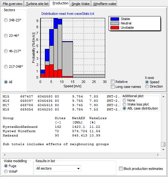
58

59 Single wake view The single wake window shows the wake of a single wake at the selected wind speed. Local wind speeds are shown at the status bar at the bottom of the program window when the mouse cursor is moved over the wake display. Clicking on the wake field will change the position of the below cross profile, which is also indicated by a dotted line in the wake field display. A more precise positioning of the profile is done by the edit boxes left of the profile view. You can zoom closer to the turbine position and optionally interpolate the results. When an edit boxes is focused, the profile position may also controlled by keyboard arrow keys combined with the shift or ctrl key. Clicking on the radio buttons to the left will change the direction of the chosen transect profile. Use the list below to select a level for horizontal profiles. The check boxes at the lower-left corner controls whether to normalise distances in the X-Y plot and whether to plot the wind profile or the wake velocity deficit. Automatic plot scaling is controlled with the plot options.

60 The plot scaling is automatic by default. You may also specify axes minima and maxima, this is useful when comparing cross profiles at different downwind positions.

61 Windfarm wake view. The wind farm wake window shows the wind field in the entire wind farm at the selected wind speed and direction. The averaging options, displayed by a mark en the checkbox at the top, will only affect the efficiency for direction plot. Zoom and pan It is possible to zoom in or out with the spin edit box above the plot. The zoom factor is calculated as 2 i/5 where i is the value in the spin edit box. Sometimes it is best to edit this number directly as it takes a while to calculate the plot and this is done each time the zoom factor change. An alternative zoom method is to press the ctrl key while scrolling the mouse wheel. Dragging the mouse with the ctrl and left mouse keys pressed will pan the wind-farm view. Speed up options Plotting the combined wind field of a big wind farm can be slow. The 'WF plot by FFT' option, i.e. acceleration by fast Fourier transforms, will speed up the plotting of a big project but not of a small one. It should not be used it in

62 combination with positive zoom, as wakes from turbines outside the view becomes invisible. Use the 'Block WF plot' option to temporarily prevent any wind-farm plotting. Adjust the view The size of the plot depends on the main window size. Plotting is time consuming because the flow has to be evaluated everywhere. Adjusting the resolution, shown in number of pixels, will speed up the process. Setting a resolution of zero will imply that Fuga interpolate in the single-wake results even for plotting - this makes most sense with a high zoom factor Checkboxes are used to add speed- and length scales plus coastline to the plot. It is also possible to adjust the colour scheme. 'New defaults' are recommended for projector displays and 'X-ray' is best for B&W printer output. Measure a distance The approximate distance and direction between two sites can be measured by dragging with the left mouse-key pressed. Press shift on the keyboard while releasing the mouse key to keep the measure on the screen. Select group, turbine site or wind profile reference point There are two ways to select a turbine site group or individual site 1. by selecting a site in the drop-down list in the 'efficiency for direction' pane 2. by clicking on the map above. Setting a checkmark at 'snap to turbine position' will move the reference point to the nearby turbine site Use the drop-down list in the top-left corner to select the height above the surface. Click the button called 'accurate position' to gain full control of the reference point, e.g. to select a point directly downwind a specific turbine Efficiency plot

63 The chart below the main plot shows the power efficiency or local speed reduction as function of wind direction. These values are normalized by the undisturbed wind speed and production of a turbine without wake effects. The direction is indicated to the left of the plot when the cursor is moved over the plot. Horizontal wind profile The wind profile along a transect - with downwind, crosswind or skew alignment - can be viewed in a separate chart. The centre position is selected by clicking on the wind-farm wake plot. Use the checkbox above the main plot to snap to a nearby turbine position. Having selected a centre position you select the alignment of the transect with the radio buttons left of the chart and adjust the extend of the transect with the spin edit buttons. Further options are Normalised distance - scale the distance with the rotor diameter 1D profile - show the profile along the transect at the select level as a curve 2D profile - show the 2D profile in a vertical plane along the transect as a coloured map Deficit only - show the wake velocity deficit instead of the corrected wind speed

64 Vertical wind profile This pane shows the vertical wind profile corrected for the combined wake effect at a position selected by a click on the map or more in the 'accurate position' dialog.

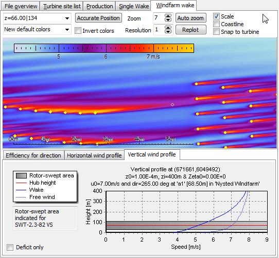
65

66 Further information File structure Fuga operations at program start up Differences between Fuga 2 and Fuga 1 Averaging options How to prepare a WAsP workspace How to prepare a WAsP windfarm file Case statistics file Roughness and stability parameters How to select a new turbine site group Data export Result table Main menu Fuga scripting Fuga speed and memory usage Software updates References

67 File structure The system is installed by unzipping the distribution file. The root directory contains: The Fuga directory includes fuga.exe and associated files plus subdirectories with WAsP data. The LUTs directory including lookup tables in the structure explained in a previous memo. Initially this directory is empty, but it will gradually expand as new cases are added. It is safe to remove part of the LUT file structure from the disc when cases are no longer needed. Fuga will direct single-wake results (*.dat files) generated by Trafalgar.exe and the associated *.par option files to the LUTs subdirectories. TIP: You can change the LUT directory path by editing the fuga.ini file in the Fuga directory, e.g. to a part of your harddisk with no backup. These voluminous files can be reconstructed at any time. The Preludium directory includes preludium.exe, trafalgar.exe and associated files. The input file for generating the prelut table, i.e. script1.txt, is not modified by Fuga, but input files for setting up a new turbines and boundary-layer cases, i.e. script2fuga.txt and script3fuga.txt, are redefined according to the Fuga user choices. Extended file structure with data for variable atmospheric stability Starting from Fuga 2.3 we need to store data for variable atmospheric stability. The stability parameter is zeta0, which is the surface roughness diveded by Monin- Obukhov length. This parameter is built into the LUT and prelut file names. We generally have more than one prelut table and more LUT tables than previously.

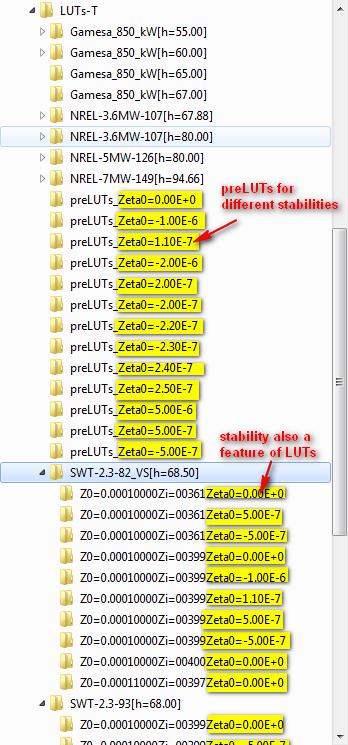
68

69 Fuga operations at program start up At the beginning of each session Fuga will scan existing LUTs directories and present available information in dropdown list on the left-hand side of the program window. It also reads the fuga.ini file in order to recover settings of the previous session. (This *.ini file is dispensable at any time). At the very first session fuga will not detect any data and therefore start to calculate the prelut table. This operation will take about 3 min, but fortunately it is only needed once.

70 Differences between Fuga 2 and Fuga 1 Fuga 1 Fuga 1 was designed for homogeneous wind farms with uniform hub heights and identical turbines at all turbine sites. A system of single-wake velocity fields and look-up tables were stored in a folder structure convenient for the Preludium and Trafalgar programs. These solutions depend on turbine hub dimension, surface roughness and boundary layer height. Input turbine power- and thrust coefficient curves were read from a WAsP wind turbine generator file (*.pow;*.wtg). The wind-farm layout was defined by a WAsP wind farm file (*.wwf), which includes turbine positions and local wind climates needed for accurate annual energy production estimates. Fuga 1 assumed all turbine hub heights to be identical, so the user had to avoid variable heights in the WAsP project generating the wind farm file. Fuga 2 Fuga 2 is designed for complex wind farms and wind-farm clusters with mixtures of turbine types. The Preludium/Trafalgar data structure is maintained, although we sometimes apply multiple folders for a single turbine if LUTs and wake data are needed for several hub heights and atmospheric stabilities. The complex wind farm layout is read from the WAsP workspace file (*.wwh). With this file format it is possible to organize turbine sites into multiple site groups nested into as many sub groups as needed. Each group, and even the individual turbine site, can have a specific turbine generator and hub height. Results are aggregated for each turbine group. Effects of turbines in neighbouring groups are included by default, but you can also model a turbine group without wake effects from neighbouring groups.

71 Averaging options Averaging options affects calculations in exported result tables turbine site list production table (new in Fuga 2.4) windfarm-wake 'efficiency for direction' plot (new in Fuga 2.4) Averaging options does not affects calculations in single-wake results windfarm-wake main plot windfarm-wake horizontal profile windfarm-wake vertical profile One reason for these limitations is that the speed-optimized wake meander model only simulates wake displacements near downwind turbine positions. The detailed wake trajectory is unknown. The averaging options appear at the top of the window when applicable. Rotor-averaged wind speed means that the inflow velocity is evaluated at seven points on the rotor and a weighted average is used for evaluating thrust and power. Without this option the inflow is evaluated at the rotor centre only. The option can be used in combination with either directional averaging method. Directional averaging Fixed wind direction is the basic and fastest method. It may however overestimate the wake centre-line velocity deficit and underestimate the width of the wake-affected region. The simple average and Gaussian average methods apply filters on the wind direction, which reduces the wake velocity deficit and increases the width of individual wakes. The width or standard deviation of these filters is specified in the input box appearing to the right of the filer-type option. Fuga actually implements two versions of these methods. The first one is based on the average of repeated calculations with wind directions distributed around a mean wind direction. The second version is based on wind directions covering the full 360 horizon, and here the filtering is done in Fourier space after FFT transforming of the raw results. The first version is used for analysing specific wind situations and the second one is used in context of AEP estimates, where winds from all directions are always available. Exported results from the result table dialogue can be calculated by either version. The final method invokes meander simulation. This is based on a stochastic model and results will differ after each simulation. To improve the uncertainty of the estimates you can repeat the simulation and use mean results. The optimum number of repeats depends on the size of the windfarm, as random variations from multiple turbines tend to cancel each other. The results for a single turbine will depend on the number of upwind turbines, so uncertainties for individual turbines will typically vary with wind direction. The same is often true for an wind farm covering an elongated area. Use the drop-down list at the top to select which simulation to display in tables and efficiency plot. The button to the right of the repeat number selector can be used to repeat the simulations.

72 A checkmark at wind direction trend will activate an additional directional averaging filter, which models the effects of variable wind direction during the sample period. The option should be set when comparing Fuga model predictions to observed turbine performance binned after an observed wind direction. In most cases this wind direction is measured at a reference mast and not at the individual turbine sites, and in this case it will be relevant also to select the spatial decorrelation option modelling the lack of correlation in concurrent wind directions at reference mast and individual turbine sites. The averaging effect decreases with wind speed and increases with distance between individual turbine sites and reference site. A project met mast will be an appropriate reference site. Open the workspace in WAsP to insert a project reference mast and select it by a click in Fuga object hierarchy. The wind direction trend and spatial decorrelation options are implemented in Fourier space. They are unavailable in the specific-wind situation but may be calculated from the 'result-table' data export.

73 How to prepare a WAsP workspace The work flow is 1. set up a WAsP project, including groups of turbines sites, a wind atlas, and wind turbine generators 2. right-click on a project object and select the do all feasible calculations or press F9 3. check that the WAsP calculations were successful, i.e. the wind farm icon in the WAsP object hierarchy should not include a warning signs 4. export the workspace file but look like this There is much more detailed information in the WAsP help file, both regarding user interface, modelling and file formats. The section called 'quick start tutorial' is recommended. Here is a list of basic operations: Modify a turbine power- and trust-coefficient curve There are two file formats for this. The old *.pow format is easiest to edit with an ASCII editor. The *.wtg format can be edited with the WAsP turbine editor. The latter file format may contain several performance tables applicable for different air density. Specify a turbine type You may (but do not have to) specify a turbine type for each turbine site. WAsP will look for a turbine assigned to the turbine group if site information is missing. If this information is missing too, then WAsP will search for a turbine type assigned to its parent group or project. The principle is to look for local information before global one. Modify a turbine height A turbine hub height in WAsP may differ from its default value in the power-curve file. Right-click on a site or turbine group and specify the real-world hub height. Add or modify turbine positions The interactive way is to right-click on an existing site to edit its coordinates or right-click on a turbine site group to add more sites. To edit lots of positions it is more convenient to import a site list which can be prepared by an ASCII editor. The format is described in the WAsP help file. Tip: Export a list from an existing group and use this as a template. Add a reference mast You can insert a reference mast for a turbine site group. In WAsP it is used as a reference for a windfarm power curve. In Fuga you can use it as a reference point for specifying wind condition at a height different from the turbine hub height(s). Reorganize turbine site groups You can insert new turbine site groups in a project and add nested sub groups. You can drag turbine sites from one site group to another. Add wind climate information Climate information is either added as a wind atlas file representative for the region or as locally observed wind statistics. Observed wind statistics are read from a file, which can be generated from time series with a tool called WAsP Climate Analyst. It is also possible to write a *.tab file which has a relatively simple format, see WAsP help file. WAsP observed wind file is assigned to a met station which specifies the met mast position and the station is assigned to a wind atlas. Wind atlas information are cleansed for local effects. The number of wind sectors used in both WAsP and Fuga depends on the number of sectors in the input wind climate. The default is to use 12 sectors. Go back to the WAsP Climate Analyst if you need to change this. Prepare terrain data This is normally done with the WAsP Map Editor. For offshore projects the roughness change at the coast line is often much more significant than terrain elevation on nearby land.

74 How to prepare a WAsP windfarm file Fuga 1 needed data in the WAsP windfarm file (*.wwf). Fuga 2 uses the more complex workspace file (*.wwh) but you can still do Fugabatch calculations based on wind farm files for simple projects with identical turbines. This wind farm file is prepared in the following way: 1. set up a WAsP project, including a group of turbines sites, a wind atlas, and a wind turbine generator 2. right-click on the site group and select the do all feasible calculations option from the popup menu 3. check that the WAsP calculations were successful, i.e. the wind farm icon in the WAsP object hierarchy should not include a warning signs but look like this 4. right-click on the site group again and select export wind farm to file from the popup menu The WAsP wind farm file contains turbine locations and, with successful WAsP calculations, also the local wind climates and annual power production estimates. Fuga version 1.0 used the even simpler WAsP site location *.txt or *.wsg file format. This file type was, however, abandoned in version 1.1, because it lacks information on wind climate and power production.

75 Case statistics file The influence of variable statistics is simplified to a statistical weighting of a selection of specific cases. Each case is specified by surface roughness z0, inversion height zi and stability parameter zeta0 and may be assigned a text identifier. The statistical frequency of occurrence for each case is given in sectors and wind-speed bins. The sectors are defined by their dividing directions, e.g , 23-46, , , in the below example. Wind-speed bins are defined by their maxima, e.g. 0-2 m/s, 2-4 m/s, 4-6 m/s, 6-8 m/s, 8-10 m/s, m/s, m/s in the below example. Example The following sample file 'casestats.txt' is included is found in the Fuga directory.

76 Roughness and stability parameters The tables provides surface roughness and stability parameters for Fuga. They describe an equilibrium offshore surfaces layer with surface roughness estimated by Charnock's equation. The wind speed U [m/s] is defined at a reference height of 70 m. The inverse Monin-Obukhov length 1/L values [m -1 ]correspond to Sathe-Gryning-Peña class limits and midpoints. 1/L very unstable unstable Table 1: Z [mm] as function of wind speed and stability. 0 near-neutral unstable neutral near-neutral stable U /L very unstable Table 2: 10 6 Zeta as function of wind speed and stability. 0 unstable near-neutral unstable neutral near-neutral stable U stable stable

77

78 How to select a new turbine site group Aggregated results shown for subgroups of turbine sites normally includes wake effects of turbines in neighbouring groups. If you want to see the performance of a group without the effects of neighbouring groups you can select the group of interest in the object hierarchy. Working with projects with three or more turbine site groups you may want to include all but one or some of these groups. This can be done by first selecting the combined set of turbines and then temporarily deactivating subgroups. You do this by right-clicking on a group.

79 Data export Data export to file or clipboard are found in the 'file' menu. Clicking on one of the 'Save...' menu items will invoke a Windows save-file dialogue. The default names are shown below but it is also possible to specify other names. Most of the results are identical to the ones shown in the user interface, but the result table has a more flexible layout. The 'Zip all' option will collect all results in a single file. The 'Copy...' options will copy results to the Windows clipboard.

80 Result table The layout of exported result tables can be modified in various ways Result type -chose whether to export wind speeds at turbine locations, with wake effects from neighbour turbines, or the corresponding power read from the WAsP power curve file. Turbine site - select data from a single site, from all sites, or the average or total from the entire windfarm Wind direction - select a range of wind directions and a increment. Choose output for each direction of just the average Wind speed - select a range of wind speeds and a increment. The results will be modelled with current averaging options.

81 Main menu You can new projects and case data form the File menu. It is possible to export results and plots to file and clipboard. The about box under the help menu provides version information for the Preludium, Trafalgar and Fuga programs.