Monsoons: Processes, predictability, and the prospects for prediction

Transcription

1 Monsoons: Processes, predictability, and the prospects for prediction P. J. Webster 1, V. O. Magana 2, T. N. Palmer 3, J. Shukla 4, R. A. Tomas 1, M. Yanai 5, and T. Yasunari 6 Journal of Geophysical Research, Volume 103, C7, June 28, 1998, 14, ,510 1 Program in Atmospheric and oceanic Sciences, University Colorado, Boulder. 2 Center for Atmospheric Sciences, National Autonomous University of Mexico, Mexico City. 3 European Center for Medium-Range Weather Forecasts, Reading, England, United Kingdom. 4 Center for Ocean-Land-Atmopshere Studies, Calverton, Maryland. 5 Department of Atmospheric Sciences, University of California, Los Angeles. 6 Institute of Geosciences, University of Tsukuba, Tsukuba, Japan. The Tropical Ocean-Global Atmosphere (TOGA) program sought to determine the predictability of the coupled ocean-atmosphere system. The World Climate Research Programme's (WCRP) Global Ocean-Atmosphere-Land System (GOALS) program seeks to explore predictability of the global climate system through investigation of the major planetary heat sources and sinks, and interactions between them. The Asian-Australian monsoon system, which undergoes aperiodic and high amplitude variations on intraseasonal, annual, biennial and interannual timescales is a major focus of GOALS. Empirical seasonal forecasts of the monsoon have been made with moderate success for over 100 years. More recent modeling efforts have not been successful. Even simulation of the mean structure of the Asian monsoon has proven elusive and the observed ENSO-monsoon relationships has been difficult to replicate. Divergence in simulation skill occurs between integrations by different models or between members of ensembles of the same model. This degree of spread is surprising given the relative success of empirical forecast techniques. Two possible explanations are presented: difficulty in modeling the monsoon regions and nonlinear error growth due to regional hydrodynamical instabilities. It is argued that the reconciliation of these explanations is imperative for prediction of the monsoon to be improved. To this end, a thorough description of observed monsoon variability and the physical processes that are thought to be important is presented. Prospects of improving prediction and some strategies that may help achieve improvement are discussed.

2 Back to the previous section Forward to the next section 2. Description of the Monsoons Ramage [1971] provided a rather strict definition of a monsoon and identified the African, Asian, and Australian regions as satisfying both a wind reversal and seasonal precipitation criterion. However, the Americas qualify as monsoon regions at least in terms of precipitation. In the following sections the various monsoon circulations will be described The Annual Cycle of the Monsoon Figure 6a. Mean upper tropospheric ( mbar) temperature (degrees Celsius) for the boreal summer (JJA), and boreal winter (DJF), averaged between 1979 and The boreal summer plot is based on calculations first made by Li and Yanai [1996]. Mean columnar temperatures warmer than --25C are shaded. In Figure 6a the horizontal distribution of the mbar layer mean temperature is plotted for boreal summer (Figure 6a left) and winter (Figure 6a right). The shaded region shows a mean temperature warmer than --26C. During summer a planetary-scale warm air mass is centered on south Asia with the maximum average layer temperature ( > --22C) over the southern Tibetan Plateau, resulting in strong temperature gradients in both the north-south and east-west directions. A warm temperature ridge exists over the North American continent, and a deep temperature trough stretches from the west coast of North America to the central Pacific. A similar trough lies over the Atlantic Ocean. The upper tropospheric flow pattern during summer identifies clearly the thermal contrast between continents and oceans [e.g., Krishnamurti, 1971a, b]. The boreal winter presents a very different structure. A much smaller section of the globe (northeast of Australia) is warmer than --26C. A

3 warm temperature ridge lies over South America, and aslightly weaker ridge covers Australia. Figure 6b. Longitude-time sections showing the annual cycle of the upper tropospheric ( mbar) temperature anomaly at 30N, 5N, 15S, and 30S. Plots are extensions of initial calculations first made by Li and Yanai [1996]. The anomalies were calculated by subtracting the annual cycle harmonic at a particular latitude from the mean columnar temperature. Figure 6b shows the longitudinal structure of the annual cycle of the upper tropospheric ( mbar)

4 temperature anomaly for the entire year along 30N, 5N, 15S, and 30S. The anomaly is calculated by subtracting out the mean zonally averaged annual cycle of the columnar mbar mean temperature along the particular line of latitude. The 30N section cuts through the temperature maximum over the Tibetan Plateau. Temperature anomalies begin to change from negative to positive in April near E. The temperature increases over Eurasia during summer are much larger than those over North America. The maximum temperature anomaly (9C) occurs in the region of the Tibetan Plateau (between 60 and 105E). Smaller maxima of mean temperature anomalies occur over North America and west Africa. In contrast, there is no appreciable change in the upper tropospheric temperature along 5N (Figure 6a top right), which is mostly over the oceans. The southern hemisphere sections at 15 and 30S are weak counterparts of the 30 N section. Compared to the > 9C anomaly found over the Tibetan Plateau, anomalies have magnitudes of only 3C at 30S. The longitude-time sections of the difference of the mean upper tropospheric ( mbar) temperature between 30 and 5N, (upper panel), 30 and 5S (center panel) and between 30N and 30S are plotted in Figure 6c. All temperature differences >6C are shaded. The reversal of the meridional temperature gradient occurs first on the south side of the Tibetan Plateau (near E) and then expands over a large area extending from Africa to the western Pacific. The temperature difference reaches maximum values (> 6 K) in July and becomes negative between September and October. Li and Yanai [1996] found that the onset of the Asian summer monsoon is concurrent with the reversal of meridional temperature gradient in the upper troposphere south of the Tibetan Plateau, as originally suggested by Flohn [1957] and later by Flohn [1968]. A small region of reversed temperature gradient may also be seen over North America. Figure 6c. Longitude-time sections showing the 5--day upper tropospheric ( mb) temperature differences between 30and 5N (left), 30 and 5S (middle) and 30N and 30S (right). Areas of differences > 6C are shaded. Northern hemisphere analysis based on initial calculations by Li and Yanai [1996]. The temperature gradients in the southern hemisphere never reverse. That is, at all times the mean temperature at 30S is cooler than at 5S because of the strongest heating occurring very close to the equator. Although Australia is a large continent, the heating is not elevated as it is over the Himalayas. Thus the major heating remains close to the north coast of the continent and close to the equator. Geostrophic adjustment is extremely rapid at very low latitudes, and it is difficult for a local temperature

5 maximum to be maintained. On the other hand, geostrophic adjustment to the elevated heating over the Himalayas is sufficiently slow to allow the development of a substantial pressure field and a warm core. However, the monsoon should be viewed in a cross-equatorial context. Figure 6c (right) shows that there are still strong cross-equatorial pressure gradients that drive the boreal winter monsoon. These gradients, not as large as those occurring in the boreal summer, are the result of the intense radiational cooling over north Asia during winter. Figure 7. Mean vertical velocity sections through the major monsoonal regions of the globe. (a) the south Asian sector (60 to 85E) during July, 1992, (b) the Australian sector (120 to 140E) during February, 1992, (c) the Americas sector (110 to 130W) during July 1992, and (d) the African sector (30 to 50W) during July Units mbar s-1. The shaded area shows upward motion. The thick line is the zero absolute vorticity contour. Data is from European Center for Medium-Range Weather Forecasts (ECMWF) initialized analyses. Based on the calculations of Tomas and Webster [1997]. Figure 7 plots the mean latitude-height cross section of the vertical velocity (upward motion is shaded) through the major monsoon areas for the months of February and July 1992 [from Tomas and Webster, 1997]. In all cases, there is very strong ascending air concentrated on the summer hemisphere side of the zero absolute vorticity contour (thick line). However, the ascending air over the Asian section during summer is of a much broader character and extends from just north of the equator to the interior of the

6 Asian continent. This wider region of ascending motion is the result of intraseasonal changes in the location of the ascending motion which "oscillates" between the low-pressure trough near or south of the equator and the south Asian continent. The vertical velocity structure of the other monsoon areas possesses patterns that are similar to oceanic Intertropical Convergence Zones (ITCZ). Figure 8. Surface pressure (solid contours) and 925--mbar horizontal wind (vectors) for (a) July and (b) February 1992 over the eastern hemisphere. The area shown is roughly the same as the monsoon region defined by Ramage [1971]. The darker shaded regions denote convection (OLR < 200 W m-2). The thick contour shows the zero absolute vorticity contour (i. e.,). The three major monsoon regions of the eastern hemisphere are easy to identify. In the boreal summer, strong clockwise flow circulates through the Indian Ocean, converging into the monsoon trough of south Asian. A weaker confluence occurs north of the equator over Africa. In the austral summer, relatively weaker confluence zones are evident over north Australia and equatorial south Africa. The thick dashed lines denote the near-equatorial troughs and the monsoon troughs farther poleward. Collectively, the system is referred to as the Asian-Australian-African monsoon system. Charts constructed using ECMWF analyses. Figure 8 provides a description of the mean boreal summer and winter monsoon circulations in the

7 eastern hemisphere. Surface isobars and 950--mbar circulation (vectors) are plotted with the mean outgoing longwave radiation (OLR) (darker shaded areas) measured from satellite superimposed to indicate the regions of mean convection. Surface isobars are also plotted with the locations of the mean surface troughs indicated by thick dashed lines. There are four major regions of convection: over south Asia and equatorial north Africa during the boreal summer and in a band extending across the Indian Ocean and north Australia during the boreal winter. During the boreal winter, there is a convective maximum in equatorial southern Africa. These convective centers define the pluvial regions of the Asian-Australian and African monsoon systems. Convection over Asia is located farther poleward than its southern hemisphere counterpart, and the circulations are not symmetrical between the seasons. Also, the circulation associated with the Asian summer monsoon is much stronger than its wintertime counterpart and possesses a concentrated cross-equatorial flow in the western Indian Ocean compared to the broader but weaker cross- equatorial flow during the boreal winter. During the summer the monsoon trough (thick dashed line) stretches across the deserts of north Africa to south Asia. A secondary and weaker trough exists near the equator in the Indian Ocean [Ramage, 1971; Hastenrath, 1994]. In the western Pacific Ocean, there is only one trough, which is closer to the equator. Similar associations are found in the austral summer, although the trough (except in the western Indian Ocean) is located closer to the equator. Troughs, in general, are associated with regions of maximum surface heating over land or with maxima in the SST over the ocean. In both seasons, though, in regions of strong cross-equatorial pressure gradients, convection lies on the equatorward side of the trough. This rule is fairly general and consistent with inertial instability processes involving cross-equatorial flow [Tomas and Webster, 1997]. However, in south Asia, deep convection appears to lie in the vicinity of the monsoon trough as well. These collocations are made up of strong intraseasonal contributions. Figure 9. Synthesis of the summer and winter monsoon divergent wind circulations. Three major components are identified: the transverse monsoon, the lateral monsoon and the Walker Circulation. The lower tropospheric mass flux and the latent and radiative heating gradients associated with each circulation are given in Table 1 in units

8 of Gkg and W m km-1, respectively. Figure 9 provides a synthesis of the divergent flow associated with the summer and winter Asian- Australian monsoon system with thick arrows denoting the major divergent circulations of the system. In the summer, there are three principal circulations: the lateral and transverse monsoons and the Walker Circulation. Most descriptions of the monsoon [e.g., Ramage, 1971; Das, 1986; Fein and Stephens, 1987] emphasize the cross-equatorial circulation of the monsoon (here referred to as the lateral monsoon component). However, there are also strong transverse components driven by longitudinal heating gradients. The first transverse circulation flows between the arid regions of north Africa and the Near East and south Asia [Webster, 1987a; Yang et al., 1992; Rodwell and Hoskins, 1996]. The second transverse circulation, the Walker Circulation, extends across the Pacific Ocean. In the summer hemisphere the ascending regions of the transverse, lateral monsoon circulations and the Walker Circulation are collocated over south Asia. During the boreal winter the same three circulations dominate but with their orientation producing common ascent over southern Indonesia, north Australia, and the western Pacific Ocean. Table 1 lists the major heating gradients associated with the component circulations shown in Figure 9 [from Webster, 1994]. The estimates of the radiational and latent heating gradients are consistent with those of Luo and Yanai [1983, 1984], Nitta [1983], and Li and Yanai [1996]. Latent heat release only takes place where there is precipitation. However, some 70% of Pacific Ocean warm pool clouds are nonprecipitating at any one time (G. Liu and J. Curry, personal communication, 1997) so that cloud enhanced radiative heating of a column can occur over broader regions than precipitation [Ramanathan, 1987; Webster, 1994]. In effect, cloudy columns tend to heat anomalously relative to clear regions by radiation alone in nonprecipitating systems or by radiation and latent heat release in precipitating systems. Thus, in the monsoon regions, the clear subsident regions in the winter hemisphere or in the eastern Pacific Ocean form strong radiational heating gradients with the more cloudy zones over the land or the warm pools. The radiative cooling is exaggerated over the arid regions to the west of south Asia during the summer (crosshatched areas of Figure 2) because of the very effective cooling to space due to the dryness of the atmospheric column. The strong contrast in radiative and latent heating between north Africa and outh Asia is the major reason for the transverse monsoon. Overall, the radiative heating gradient is about half as large as the latent heating gradient in the lateral monsoon and the Walker Circulation, although somewhat larger in the transverse monsoon.

9 The three major circulations of Figure 9 constitute the majority of the lower tropospheric divergent mass flux. Table 1 also lists the mass fluxes associated of the component circulations. The mass flux is calculated from the average lower-tropospheric divergent wind speed in the layer mbar and across a km sector through the center of the circulation stream. To gain an appreciation of the divergent wind flux, it is useful to compare the values with oceanic transports. In the ocean, a 1--m s-1 current in a 100--km wide by 0.5--km deep layer (roughly the scale and magnitude of the Somalia Current) provides a mass flux of 50 Sv (50*106 m3 s-1) or 50 Gkg s-1. The atmospheric equivalent to this mass flux would be produced by a divergent wind speed of 10 m s-1 flowing through the km atmospheric section defined above. Figure 10. Annual cycle SST (degree Celsius) as a function of time of year along (a) 12.5N, (b) the equator, and (c) 15S across the Indian Ocean. Dark shaded regions indicate the location of land masses in the sections relative to the map at the bottom of the panels. The dashed lines across the maps denote the latitude along which the longitude-time sections were constructed. The strongest divergent atmospheric flux appears to be associated with the transverse and lateral monsoon circulations of the boreal summer. Using mean summer atmospheric data for the Indian Ocean gives a divergent flux of 2.5*104 Sv or 25 Gkg s-1. This divergent flux is about one third of the total

10 cross-equatorial flux of the Findlater Jet [Findlater, 1969b]. The remainder of the mass flux is associated with the rotational part of the wind field. Thus the mass flux associated with the Somalia Current in the ocean and the total mass flux of the atmospheric Findlater Jet are roughly equivalent. In the boreal summer the divergent longitudinal flow of the Walker Circulation is about half as large as either of the monsoon components. However, during the boreal winter the divergent mass flux of the Walker Circulation is of a comparable magnitude. Throughout the annual cycle the SST in the Indian Ocean undergoes an interesting progression. Figure 10 shows three longitude-time sections across the Indian Ocean for the year In the most general sense the SST maxima should lag behind the annual cycle of solar heating by about 2 months. However, a closer scrutiny of Figure 10 shows that this is not the case. The northern Indian Ocean (Figure 10a) remains warm throughout most of the winter, slowly increasing to a maximum of 30C in late June. Substantial cooling occurs in the vicinity of Somalia commencing in June at the equator and during July in the Arabian Sea. The cooling is associated with both upwelling and evaporation accompanying the freshening winds of the southwest monsoon [Knox, 1987]. The southern Indian Ocean appears to undergo a more regular annual cycle. However, the SST maximum occurs some 5 months after the southern hemisphere summer solstice. Furthermore, the maximum SST in the boreal winter actually occurs even farther south near 15S in the vicinity of 60E, where, during February, temperatures exceed 30C. However, during this season and at these longitudes, maximum convection occurs equatorward of the maximum SST because of dynamical constraints [e.g., Walliser and Somerville, 1994; Tomas and Webster, 1997]. Figure 11a.(a) Orography and the south Asian summer monsoon. Orographic structure of the eastern hemisphere (units are 102 m). The Indian Ocean is surrounded by the East African Highlands to the west and the Himalayan Mountains to the north. Australia, on the other hand, is devoid of major orography. Orography with elevations >1 km are shaded.. Figure 11a displays the major orographic features of the eastern hemisphere. The Indian Ocean is bordered to the west by the East African Highlands and to the north by the Himalayas and the Tibetan

11 Plateau. Australia is effectively devoid of major orographic features. Figure 11b provides firm evidence that the Himalayas and the Tibetan Plateau play an important role in the evolution of the boreal summer monsoon [e.g., Yanai et al., 1992; Flohn, 1957]. Using data from the First Global Atmospheric Research Program (GARP) Global Experiment (FGGE) and data collected from the Qinghai-Xizang Plateau (Tibetan Plateau) Meteorology Experiment (QXPMEX), Yanai et al. [1992] studied the seasonal changes in the large-scale circulation, thermal and moisture distributions over the Tibetan Plateau and surrounding areas. Figure 11b plots the seasonal change of the large-scale vertical circulation along the 90E meridian for the 9-month period from December 1978 to August The shaded area denotes upward motion. In general, air above the Tibetan Plateau is always warmer than the air at the same levels in the surrounding areas at the same latitudes. During the winter and early spring the flow is strongly subsident to the south of the Plateau. Later in the spring, there is relatively weak upward motion to the south of and adjacent to the Plateau. Ascent becomes stronger and extends longitudinal from 5 to 45N. Yanai et al. [1992] also calculated the circulations in the height-longitude plane along 32.5N. Whereas the circulation over the Plateau is quite similar to that shown in Figure 11b, the lateral extent of the circulation is somewhat larger. Until June the regions to the east of the Plateau are dominated by strong subsidence, which Yanai et al. [1992] relate directly to the elevated heat source. After June, ascent becomes more general expanding both to the east and the west of the mountains. Compared to the Asian-Australian monsoon, the African monsoon is relatively weak. Figure 8 indicates onshore flow into west Africa during the boreal summer and a return flow during winter. Over equatorial Africa, there are two distinct rainy seasons. Perhaps the greatest difference between the African monsoon system (and the monsoons of the Americas) and the Asian summer monsoon is the lack of elevated heating associated with terrain as large and extensive as the Himalayas.

12 Figure 11b. (b) Orography and the south Asian summer monsoon. Mean monthly latitude-height sections along 90E from December 1978 through August Arrows show the streamlines in the meridional-height plane. Black region indicates the Himalayas. Shaded region denotes upward motion. From Yanai et al. [1992].. In Figure 6b, there appear to be only two reversals of the latitudinal temperature gradient. These occur between south Asia during the boreal summer and, with a substantially reduced magnitude, over North America. Although only smaller in extent and in height, the Rockies provide an elevated heating similar to the Tibetan pattern. As a result, there exists a monsoon circulation in North America. Figure 12 shows the 925--mbar wind field, mean sea level pressure, and the OLR for July 1992 and January During the boreal summer, there is a strong southerly flow into Mexico and the United States from the Gulf of Mexico. The flow differs from classical monsoon patterns in that the flow is not cross-equatorial. Two pressure troughs exist: one near the equator associated with the ITCZ and a second over northern Mexico and the southwestern United States.

13 Figure 12. Surface pressure and 925 mbar horizontal wind for (a) July and (b) January 1992, for the Americas. The darker shaded regions denote convection (OLR<200 W m- 2). The thick contour denotes the zero absolute vorticity contour (i.e., ). Though somewhat weaker than Asian-Australian, the North and South American monsoons are discernible as the reversing currents flowing into Mexico during July and into central South America during January. The thick dashed lines indicate near-equatorial troughs and monsoon troughs farther poleward. Charts were constructed using ECMWF analyses.. The rainy season over northwestern Mexico and the southwestern United States is characterized by a maximum in precipitation during the months of July, August, and September, which accounts for 60--

14 80% of the annual precipitation. The circulation that leads to the establishment of the summer rainy season exhibits a monsoonal character, with a reversal in the surface and midtropospheric winds. The term "Mexican monsoon" has been used to describe the seasonal cycle of temperature and precipitation in analogy with the best-known Asian monsoon. The shift in the midtropospheric winds from westerly to easterly led Sellers and Hill [1974] to think that the moisture source for the Mexican monsoon was the Gulf of Mexico. However, Douglas et al. [1993] and several others argue that the Gulf of California and the eastern Pacific act as the main moisture sources for deep convection during summer. The higher precipitation over the western Sierra Madre, compared with the eastern side, appears to confirm this. Recent scientific field experiments show that the Sierra Madre over western Mexico, particularly important in the formation of the mesoscale convective systems and the generation of summer precipitation, is a region where moist air converges [Reyes et al., 1994]. Various studies have attempted to link the annual cycle of the eastern Pacific Ocean warm pool SST (off the coast of southern Mexico) with the Mexican monsoon [Mitchell and Brown, 1996]. Warm SSTs spread up along the western coast of Mexico from May through July when humidity in the region reaches peak values. This humid air may be drawn inland by surface winds and low pressure, where it results in intense convective activity related to orography. The onset of the North American monsoon is related to a major change in the wind field and the quasisimultaneous initiation of the rainy season. The onset occurs along with a transition from warm and dry to cool and moist conditions. Convective activity over the Gulf of California and northwestern Mexican region exhibits fluctuations related to intensification in the low-level jet. The wind over this region shows large departures from a uniform southerly flow known as "gulf surges," whose origin is as uncertain as the origin of the active and break periods of the Indian monsoon. The flow over South America during the austral summer is marked by a strong cross-equatorial flow from the western Atlantic Ocean that flows toward a monsoon trough located between 25 and 30S. To a large degree, the flow is reminiscent of the south Asian summer monsoon. Although the flow is not as strong as the south Asian case, it is cross-equatorial in contrast to the North American monsoon. The warm season corresponds to a well-defined rainy period associated with continental-scale vertical motion. During this season the upper troposphere "Bolivian high" develops [Virji, 1981], similar to the Tibetan high, maintained by the latent heating. As in the Tibetan Plateau case, the surface sensible heating over the central Andes plays a predominant role in warming up the midtroposphere during the premonsoon period. Although there is not a complete reversal of flow in the South American continent, a seasonal shift in the inflow of the eastern side is observed. This includes a reversal in the cross-equatorial flow over the northern part of the Amazon basin and the merging of the subtropical and the midlatitude upper troposphere jets during the summer season. 2.2.Variability of the Monsoon Besides possessing the largest annual amplitude of any subtropical and tropical climate feature, the monsoons also possess considerable variability on a wide range of timescales. Within the annual cycle there are large-scale and high-amplitude variations of the monsoon. On timescales longer than the annual cycle the monsoon varies with biennial, interannual, and interdecadal rhythms. In the following sections an attempt is made to describe these variations Intraseasonal variability.

15 Figure 13a. Climatological times of the onset of the south Asian summer monsoon. Constructed using data from data in Ramage [1971], Das [1986], and Hastenrath [1994].. Perhaps the most important subseasonal phenomenon of the monsoon is the onset of the monsoon rains. Forecasting the timing of the onset is critical as it defines the ploughing and planting times in agrarian societies in the monsoon regions. Figure 13a shows isopleths of the average dates of the commencement of the monsoon rains [Ramage, 1971]. The first rains of the monsoon occur over Burma and Thailand in middle May and then progress generally to the northwest, so that by middle June, rains have advanced over all of India and Pakistan. However, during any one monsoon season the dates of the commencement of the monsoon in a particular location are quite variable. Furthermore, the onset can be very rapid.

16 Figure 13b. Space and time distributions of the intraseasonal variability of the monsoon for the year (left) Longitude-time sections of the 850--mbar meridional velocity component (V) along 0--90E averaged between 5N and 5S. Dark contour denotes zero speed. (middle) 850 mb zonal velocity component (U) along averaged between 5 and 10N. Dark contour denotes zero speed. Darker shading shows westerly winds (U > 0) (right) 850--mbar zonal velocity component (u) along averaged between 5S and 10S. Note the rapid onset of the monsoon almost concurrently in the eastern Indian Ocean and over south Asia. During both summer and winter there are periods of strong westerly winds. In the boreal summer these westerlies extend almost to the date line. National Center for Environmental Prediction (NCEP)-National Center for Atmospheric Research (NCAR) reanalyzed data was used in the analyses. All data are 5--day running means with units of ms-1.. Figure 13b shows the mean longitude-time sections of the cross-equatorial meridional flow between 0 and 90E and the zonal flow averaged between 5--15N and 5--15S from 0 to 180E, respectively. The longitudinal structure of the 850--mbar meridional flow (Figure 13b, left) shows a distinctive geographical structure. Strong winds occur east of 40E, which is the longitude of the East African Highlands. The strong southerlies correspond to the Findlater Jet mentioned previously. The onset of the summer monsoon can be recognized by the rapid acceleration of southerly winds in the western Indian Ocean in early June. Winds accelerate from weak northerlies to strong southerlies (>9 m s-1) within a week. The onset over the north Indian Ocean is manifested by an equally rapid acceleration of the zonal

17 flow (Figure 13b). In the first few days of June, strong westerlies establish themselves between 45and 100E. Following the onset, westerly winds dominate the region until October. During this period the westerlies are far from steady. In mid-june, mid-july, and early September, winds accelerate to strengths >10 m s- 1 for periods of days to weeks. The westerlies extend eastward into the northwestern Pacific Ocean to E. These extensions are made up of active periods of the south Asian monsoon. The westerlies decrease steadily through October. Although the winds in the longitudinal span become easterly, there are a number of westerly surges even in November. The onset of the Australian summer monsoon occurs as suddenly as the Asian monsoon. In December, weak westerlies (Figure 13b, right) are replaced by broad and strong westerlies extending from the central Indian Ocean to the date line. The Australian monsoon, too, is characterized by spasmodic westerlies that extend to the date line with distinct lulls in between. The surges of the Australian monsoon correspond to major westerly wind bursts in the western Pacific Ocean [McBride et al., 1995], which have considerable influence on the structure of the Pacific warm pool [Lukas and Lindstrom, 1991]. Figure 14. Time sections of the 850--mb wind from November 1992 to April 1993 for certain key areas in the monsoon regions. (a) Locations of the time sections. (b) Zonal wind component for the Australian sector (10S to the equator and 120 to 150E) and the

18 Asian sector (10 to 30N and 60 to 120E) for the period November, 1991 through March, Active periods are clearly defined as peaks in the monsoon westerlies. Breaks are the minima in the monsoon westerlies. (c) Zonal wind component in the African monsoon region (5-15N and 0 to 40E) and the meridional wind component in the Somalia section (10S to 20N and 40 to 55E). NCEP-NCAR reanalyzed data were used in the analyses. All data are 5--day running means with units of ms-1.. Figure 14 shows a time sequence of the areal average of the 850--mbar zonal wind component over representative areas (Figure 14a) in the summer monsoons of south Asia (0--20N, E), Australia (0--15S, E), and equatorial north Africa (5-15N, 0--40E). In addition, the 850--mbar meridional wind component for the Somalia-western Indian Ocean region (10S-20N, 40-50E) is plotted. The Australian sector is the same as used by McBride et al. [1995]. The Australian and Asian regions exhibit broad areas of westerlies during the respective summers. In each region the westerlies show considerable variability with distinct lulls in intensity lasting a number of days to weeks. The lulls correspond to the breaks in the monsoon flow, while the peaks are the active periods of the monsoon. Within each summer monsoon regime, there are three or four active and break sequences. The major difference between the two monsoon regions is the degree of variability. The south Asian monsoon shows variations that are 3 m s-1 on a background flow of about 8 m s-1. On the other hand, the north Australian monsoon variations of the basic flow are about 5 m s-1 on a mean of 5 m s-1. The meridional flow in the western part of the Indian Ocean has variations in form that are similar to the Asian sector westerlies. Associated with the accelerations of the westerlies are pulses in southerly cross-equatorial flow. The African summer westerlies are weaker than both the Australian and Asian flow. Figure 15. Latitude-time sections of satellite microwave sounding unit (MSU) rainfall for (a) 1992 and (b) 1993 boreal summer seasons along 60E (Figures 15a and 15b, top) and 90E (Figures 15a and 15b, bottom). Data is a combined product from MSU data

19 and surface precipitation data (D. Lawrence, Program in Atmospheric and Oceanic Sciences: University of Colorado, Boulder, unpublished analyses). Shaded areas denote the periods shown in Figure 17.. Figure 15 plots latitude time sections of microwave sensing unit (MSU) precipitation for 1992 and 1993 along 60E (Figures 15a and 15b, top) and 90E (Figures 15a and 15b, bottom, Bay of Bengal) from April to November between 40N and 30S. The evolution and intensity of the precipitation events are very different between the eastern and western Indian Oceans. In the eastern section, there are two primary locations of precipitation. The first is to the south of the equator, and the second is farther north in the central Arabian Sea. There is some evidence of migration between these two locations. In the west, on the other hand, the convection appears to have the same two major locations and two forms of migrations. Precipitation occurs near the equator and moves northward to a location over the northern Bay of Bengal, where it exhibits variability on day timescales. With the northward propagations are propagations into the southern hemisphere. These are characterized by "Y" patterns emanating from the equator. The southward propagations which appear in both 1992 and 1993 are responsible for the secondary precipitation maximum to the south of the equator in the eastern Indian Ocean. Figure 15 shows data for 2 years which exhibit considerable differences, especially in the western Indian Ocean. In 1993, following the onset of the monsoon, major precipitation stays close to the equator. In the eastern Indian Ocean the distributions are quite similar between the years with Y patterns occurring in both. The different loci of the convection and the northward migrations were first noted by Keshavamurty et al., [1980] and Sikka and Gadgil [1980] and were discussed in a number of studies [e.g., Webster and Chou, 1980a, b; Webster, 1983a; Goswami and Shukla, 1984; Srinivasan et al., 1993]. Sikka and Gadgil [1980] and Gadgil and Asha [1992] noted that the migrations were longitudinally coherent from one side of the Indian Ocean to the other. However, all of these analyses concentrated on the northern hemisphere and did not encounter the southward propagations from the equator in the east. Whereas all of the analyses indicate that there are migrations or oscillations in the location of convection, none of them noted the great differences that occur from one side of the Indian Ocean to the other. Clearly, the intraseasonal variability of the monsoon in the Indian ocean is very complex. In the simplest sense, there are three intraseasonal monsoon phenomena that occur in Figure 15. These are the "onset" of the summer monsoon and active and break periods within the season. The onset of the monsoon appears to have many definitions, varying from a gradual increase in humidity and the commencement of precipitation [Das, 1986] to the sudden establishment of a "monsoon vortex" [Krishnamurti et al., 1990] in the northern Indian Ocean. The circulation changes do have considerable interannual variability with sustained rains commencing in different parts of south Asia at different times. During 1992, however, convection rapidly progressed northward in May or early June at 60and 90E. The active and break periods of the monsoon are characterized by precipitation maxima and minima over south Asia or northern Australia, depending on the season. These periods are thought be associated with shifts in the location of the monsoon trough. During the monsoon break the monsoon trough moves northward to the foot of the Himalayas, resulting in decreases of rainfall over much of India but enhanced rainfall in the far north and south [e.g., Ramanadham et al., 1973]. These anomalies are large scale and extend across the entirety of south Asia. Breaks and active periods vary in duration and may last between a few days and weeks. Active and break periods of the north Australian summer monsoon appear to have a different signature

20 from those of the northern hemisphere summer. Rather than exhibiting north-south oscillations, the convection appears to propagate more zonally [McBride, 1983]. However, the space scales and timescales of the events are quite similar. The active periods in the north Australian monsoon possess a similar longitudinal spread to their boreal summer counterparts. However, the austral summer active periods often extend to the mid-pacific Ocean, where they are termed major westerly wind bursts [McBride et al., 1995; Davidson et al., 1983; Fasullo and Webster, 1998]. Hendon and Zhang [1997] note that there are large differences in the frequency of active and break periods from year to year. Similar interannual differences have been noted in the Asian summer monsoon. The time sections of Figure 15 define large-scale and coherent structures of the active and break periods. To isolate the different atmospheric circulations that occur during these events, composites of active and break periods that occurred between 1980 and 1993 were created (Figure 16). The criteria used to define the active and break periods and the dates of the periods themselves are shown in the appendix. Three to four active periods were identified each boreal summer. Figure 16 shows the differences between active and break periods in the rotational part of the flow at 850 mbar (Figure 16a), the divergent part of the flow at 850 mbar (Figure 16b), and the precipitation (Figure 16c). The composites show that during an active period the cross-equatorial monsoon vortex is far stronger than during a break period. There is also enhanced convergence in a band extending from the Arabian Sea to the South China Sea. Within this band, there is enhanced convection. To the north and south of the enhanced precipitation, there are bands of reduced rainfall. In terms of the components identified in Figure 9 both the transverse and lateral components of the monsoons accelerate during active periods. During breaks these circulations are diminished.

21 Figure 16. Composites of active and break periods of the summer south Asian monsoon. (a) The 850--mbar rotational wind component (m s-1) and (b) the 850--mb divergent wind component (m s-1). Thick dashed line indicates line of maximum anomaly convergence. (c) The precipitation (mm d-1) between active and break periods of the summer Asian monsoon for the period Active periods are accompanied by a strong cross-equatorial flow in the eastern Indian ocean, stronger westerlies, increased convergence, and greater precipitation in the north Indian Ocean. During break monsoon periods there is a secondary precipitation maximum just north of the equator. Wind data are from ECMWF operational analyses for the period Active and break periods are defined in the appendix. Precipitation data is a combined product from MSU data and surface precipitation data (D. Lawrence: Program in Atmospheric and Oceanic Sciences, University of Colorado; Boulder. Unpublished analysis.).

22 The composites of Figure 16 suggest a rather simple set of distributions of the fields of dynamics and precipitation in active and break periods of the south Asian monsoon. Composites of the transitions between the active and break periods [e.g., Fasullo and Webster, 1998] show an orderly transition. However, individual active and break periods and the transition in between are much more complex. To illustrate this complexity, Figures 17a and 17b show a sequence of 850--mbar wind flow and precipitation charts for an active and break period, respectively.

23 Figure 17. Detailed analyses of 850--mbar velocity (vectors) and precipitation (shaded areas) for two sequences during the summer of 1992 from late July to early August within the dashed rectangles of Figure 15. (a) Four days of an active period (b) four days of a break period. The thick black contour shows the zero absolute vorticity at 850--mbar. See appendix for definition and the timing of the active and break periods. Note the complexity of the individual active and break periods in sharp contrast to the composite reconstructions shown in Figure 16.. The MSU precipitation is shown as the shaded regions. The contours are isotachs, and the thick line is the zero absolute vorticity contour at 950 mbar. The period during which the two sequences were made is shown in Figure 15. The active period (Figure 17a) shows widespread precipitation over the eastern Arabian Sea and the Bay of Bengal. Throughout the 4 day period, winds in excess of 20 m s-1 spread across the north Indian Ocean. In the southern hemisphere, strong southerly winds extend across the entire Indian Ocean. During the break period (Figure 17b) the winds are much weaker, especially in the Bay of Bengal. Precipitation extends across south Asia and into the northwestern Pacific Ocean. Furthermore, the cross-equatorial flow is concentrated in the western Indian Ocean. although considerably weaker. The precipitation is generally located farther equatorward, weaker and less widespread than during the active period. However, the day-by-day patterns are much more complicated than the composite analyses. The association of active and break periods of the monsoon with the day Madden Julian Oscillation (MJO) [Madden and Julian, 1972, 1994] is unclear. The MJO can be defined as a day oscillation in the large-scale circulation cells that move eastward from at least the Indian Ocean to the central Pacific Ocean. As discussed above, there is abundant evidence of frequency peaks in south Asian rainfall and wind in the same period band as the MJO [Murakami, 1976; Yasunari, 1979, 1980, 1981; Sikka and Gadgil, 1980; Wang and Rui, 1990; Julian and Madden, 1981;

24 Madden and Julian, 1972, 1994]. However, climatologically, the most active period of the MJO (at least in its equatorial manifestation) is in the boreal fall and winter (November through March). Oscillations of similar timescales in the summer monsoon often occur as northward migrations of convection [e.g., Murakami, 1976; Sikka and Gadgil, 1980; Hartmann and Michelson, 1993; Wang and Rui, 1990] or as a combination of northward and southward loci following an initial eastward migration [Wang and Rui, 1990]. Examples of these latter migrations were shown in Figures 15 and 17a and 17b. The association in the Australian monsoon appears to be more straightforward. McBride [1983], Hendon and Liebmann [1990a, b], and McBride et al. [1995] show close associations between the MJO and the active and break periods of the Australian monsoon. In the absence of a physical explanation for the MJO [Madden and Julian, 1994] it is equally fair to state that the MJO is a result of an inherent instability of the coupled ocean-atmosphere monsoon flow than to say that the active and break periods of the monsoon are the result of the MJO Longer-term variability. The wavelet analyses of Figure 3 suggest the existence of interannual variability in the monsoon and also relationships with other major features of the coupled ocean-atmosphere system. The monsoon exhibits variability in three major frequency bands longer than the annual cycle. These are the biennial period (first discussed by Yasunari [1987, 1991] Rasmusson et al. [1990], and Barnett [1991], the multiyear ENSO frequency (originally discovered by Walker [1923], and interdecadal variability Biennial variability and the monsoon year. The interannual variability of monsoon rainfall over India and the Indonesian-Australian region shows a biennial variability during certain periods of the data record (Figure 3b). It is sufficiently strong and spatially pervasive during these periods to show prominent peaks in the 2-3--year period range, constituting a biennial oscillation in the rainfall of Indonesia [Yasunari and Suppiah, 1988] and east Asia [Tian and Yasunari, 1992; Shen and Lau, 1995] as well as in Indian rainfall [Mooley and Parthasarathy, 1984]. Thus the biennial oscillation, referred to as the tropospheric biennial oscillation (TBO) in order to avoid confusion with the stratospheric quasi-biennial oscillation (QBO) (initially discovered by Reed et al. [1961] and Veryard and Ebdon [1961]) appears to be a fundamental characteristic of Asian/Australian monsoon rainfall. Yasunari [1989] has suggested that the TBO and the stratospheric QBO may have a coherent link. However, the significance or the form of the link is yet to be fully understood. The rainfall TBO appears as part of the coupled ocean-atmosphere system of the monsoon regions, increasing rainfall in one summer and decreasing it in the next. The TBO also possesses a characteristic spatial structure and seasonality as well. Meehl [1987, 1994a] stratified ocean and atmospheric data relative to strong and weak Asian monsoons. He found specific spatial patterns of the TBO with a distinct seasonal sequencing. Anomalies in convection and SST migrate from south Asia toward the southeast into the western Pacific of the southern hemisphere following the seasons.

25 Figure 18. Biennial coherence between the SST in the central Pacific (equator and 170E) and the zonal wind component over the global oceans represented by harmonic dial vectors. The maximum biennial SST-zonal wind correlation (0.7) is at the base point. The downward (upward) pointing arrows signify in phase (1 year out-of-phase) relationships. From Ropelewski et al., [1992].. Figure 18 [Ropelewski et al., 1992] shows that the lower-tropospheric wind field associated with the TBO in the SST fields possesses an out-of-phase relation between the Indian Ocean and the Pacific Ocean basins. An eastward phase propagation from the Indian Ocean toward the Pacific Ocean is suggested [Yasunari, 1985; Kutsuwada, 1988; Rasmusson et al., 1990; Ropelewski et al., 1992; Shen and Lau, 1995], which links monsoon variability with low-frequency processes in the Pacific Ocean [Yasunari and Seki, 1992]. While anomalies associated with the TBO move and develop continuously from the boreal summer to the following austral summer season, they become stationary and decay between the boreal winter and the following boreal summer Yasunari [1996]. This temporal asymmetry of the TBO is evident in the time series of the Indian monsoon rainfall anomaly (Figure 19a) during the boreal summer and the equatorial western Pacific SST in the subsequent winter (January) [Yasunari, 1990]. Figure 19b [Yasunari, 1990] presents a systematic display relation of lag correlations between the Indian monsoon rainfall and SST in the equatorial western and eastern Pacific. Y(0) denotes the reference year while Y(-1) and Y(+1) refer to the year before and after. The lag correlation gradually increases after the summer monsoon season and reaches its maximum in the following northern winter in the period between Y(0) and Y(+1) both in the western and the eastern Pacific but with opposite signs. A similar feature of lag correlation relationships can also be found for the east Asian monsoon rainfall [Shen and Lau, 1995] suggesting that the Asian summer plays a significant role in forming the anomalous state of the ocean-atmosphere system in the Pacific Ocean. That is, a strong (weak) summer monsoon tends to lead a La Nina (El Nino) in the equatorial Pacific in the later seasons of the year. These diagnostic studies are corroborated by the modeling studies of Matsumoto and Yamagata [1991], Webster [1995], and Wainer and Webster [1996].

26 Figure 19a. Time series of the Indian monsoon rainfall (thick gray line) and the upper ocean temperature at 20 m (dashed line) and 100 m (thin line) averaged along 137E between 2 and 10N in the following January. From Yasunari [1990].. Figure 19b. Lagged correlations between the Indian monsoon rainfall anomaly and the SST anomaly in the western Pacific Ocean (0-8N, E; solid curve) and the

27 eastern Pacific Ocean (0--8N, W; dashed curve). Y(0) denotes the reference year, and Y(-1) and Y(+1) refer to the year before and after the reference year. From Yasunari [1990].. Another significant feature of Figure 19b is the near-zero correlation between the boreal spring and early summer during which there is a change in the sign of correlation. The same persistence and tendency of lag correlations in the seasonal cycle is also apparent in other indices of the ocean--atmosphere system (e.g., SST, SOI, etc.) as noted by Yasunari [1990] and Webster and Yang [1992]. The implication of the changes in correlation is that an anomalous state of the ocean-atmosphere system in the equatorial Pacific Ocean basin tends to decay in the boreal spring and another state with opposite sign tends to develop at the time of the next summer Asian monsoon onset. Webster and Yang [1992], Webster [1995], and Torrence and Webster [1998] refer to this prominent feature of boreal spring as the predictability barrier of climate system in the tropics. In other words, the biennial oscillation in the ENSO-monsoon system is an oscillation which tends to have a strong seasonality with the maximumamplitude phase in boreal winter and the node phase in boreal spring to early summer. Yasunari [1991] used the changes in the persistence of atmospheric character during the boreal spring to define a unit year which starts from the boreal spring and ends at the following boreal spring. This was termed the "monsoon year" and provides a clear demarkation of the character of annual variability. It also appears to have a very wide geographical extent. Thus the concept appears useful not only for the Asian- Australian monsoon region but also for tropical regions extending from Australia to the Americas and Africa [Yasunari, 1991]. Yasunari's [1990, 1991] study of the decoupling of the annual cycle during the boreal spring is based on data from the last two decades. If the study is enlarged to longer periods [e.g., Balmaseda et al., 1995; Torrence and Webster, 1998], there are periods where the boreal spring change in autocorrelation either does not occur, is weaker or occurs at a different time of the year. Yasunari's [1990, 1991] transitions tend to match the periods of strong ENSO variance prior to 1918 and between 1965 and 1990 (compare figure 3). Explanations for the TBO in the Asian-Pacific monsoon coupled system fall into two main groups. The first group sees the TBO as resulting from feedbacks in the seasonal cycle of the atmosphere-ocean interaction in the warm water pool region. The second group of hypotheses refers to the impact of land surface processes, especially snow cover over Eurasia during the previous winter and spring. Nicholls [1983] noted a seasonal change in the feedback between the wind field and surface pressure. In the monsoon westerly (wet) season the wind speed anomaly is negatively correlated to the pressure anomaly, while in the easterly (dry) season it is positively correlated. The wind speed anomaly, on the other hand, is negatively correlated to the SST change throughout the year through physical processes such as evaporation and mixing of the surface ocean layer. Nicholls suggested that a simple combination of these two feedbacks in the course of the seasonal cycle induces an anomalous biennial oscillation. Meehl [1987, 1989, 1994a] substantiated Nicholls' hypothesis but focused on the memory of oceanic mixed layer. That is, when large-scale convection over the warm water pool region, associated with seasonal migration of ITCZ and the monsoon, is stronger (weaker), the SST will eventually become anomalously low (high) through the coupling processes listed above. The anomalous state of the SST, thus produced, may be maintained through the following dry season and even to the next wet season. In turn, the SST anomaly produces weaker (stronger) convection. In this class of hypotheses the ocean-- atmosphere interaction over the warm water pool appears to be of paramount importance. However, some important aspects of interannual variability of the monsoon coupled system (e.g., asymmetric

28 seasonal evolution of anomalies from boreal summer to winter and winter to spring as shown in Figure 19b) are not specifically explained Interannual variability and monsoon-ensorelationships: It is clear from the statistical analyses shown in section 1 that the monsoon, together with the coupled ocean-atmosphere system of the Pacific Ocean, undergoes oscillations on interannual (3--7 years) timescales. Specifically, when the Pacific Ocean SST is anomalously warm, the Indian rainfall is often diminished in the subsequent year. The correlation of the AIRI and the SOI over the entire period is while relationship with the SST in the eastcentral Pacific Ocean is slightly greater at [Torrence and Webster, 1998]. Shukla and Paolina [1983] were able to show that there was a significant relationship between drought and ENSO. Table 2 summarizes the relationships between the Asian- Australian monsoon rainfall and the state of ENSO in the equatorial Pacific Ocean and updates the Shukla and Paolina [1983] relationships. In fact, all El Nino years in the Pacific Ocean were followed by drought years in the Indian region. Not all drought years were El Nino years, but out of the total of 22 El Nino years between 1870 and 1991, only two were associated with above average rainfall. La Nina events (i.e., the opposite phase of the SOI) were only associated with abundant rainy seasons, and only two were associated with a monsoon with deficient rainfall. A large number of wet years were not associated with cold events, just as many drought years were not associated with warm events. Although the relationship is far from perfect, it is clear that the monsoon and ENSO are related in some fundamental manner. Very similar relationships occur between the north Australian rainfall and ENSO. Webster and Yang [1992] used a dynamic criterion to differentiate between strong and weak monsoons. A monsoon-wide precipitation criterion would be ideal, but precipitation data is inhomogeneous and is notoriously subject to local effects and compilations of long-term precipitation data which is only available over Indian and north Australia. The aim was to provide a monsoon index that was representative over the scale of the monsoon and that had a solid dynamic basis. Such a quantity is the vertical shear in the monsoon regions, which is assumed to have a fundamental relationship with the total heating in the atmospheric column. M is a measure of the area-and time-averaged vertical shear given by

29 where U i is the monthly (or seasonal) value of the zonal velocity component at a point and at pressure level i and U i bar is the long-term average monthly zonal velocity component at the same point and level. The overbrace indicates an areal average.

30

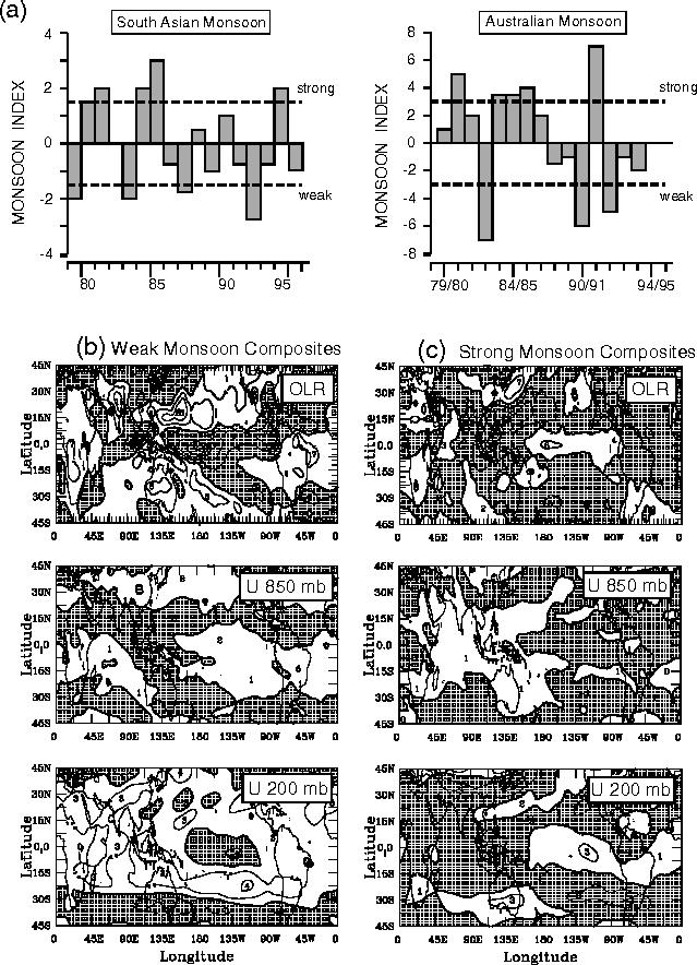
31 Figure 20. (a) Mean seasonal monsoon index (M) calculated in the south Asian and the north Australia sectors defined in Figure 14. The index is the difference between the zonal flows at 850 mb and 200 mb. (b) Composite anomaly fields calculated in the manner of Webster and Yang [1992] for the "weak" south Asian monsoon years defined in Figure 20a. (c) Same as Figure 20b but for the "strong" monsoon years. The anomaly fields show the composite differences from the long-term June-July-August average. The OLR is in anomaly (W m-2). Shaded regions denote negative anomalies. Data are from NCEP/NCAR reanalyses.. Figure 20a shows seasonal M values for the summer monsoons of south Asia and north Australia. The areas over which the index is calculated are shown in Figure 14a. Large differences are apparent in the strength of the circulations in the two regions. Strong and weak monsoon seasons are said to exist when the shear index is outside the limits < M < 1.5 for the Asian monsoon and --3 < M < 3 for the Australian monsoon. To date, detailed analyses of anomalous monsoon years are restricted to the current period of National Centers for Environmental Prediction (NCEP) reanalysis, Eventually, when the NCEP reanalysis is complete, it will be possible to compare monsoon circulations for the period of 1952 through the current year using data from the same model. Goswami, et al. [1997] have tried to identify the scale of the Indian monsoon variability using analyzed precipitation [Xie and Arkin,1996] for the period 1979 to 1995 and showed that on interannual time scale, the precipitation tends to vary simultaneously over a region larger than the Indian continent. They defined an extended Indian monsoon precipitation (EIMR) index as precipitation averaged over the region between E and 10-30N. They also showed that this index of Indian monsoon correlates well with a measure of the monsoon Hadley circulation (MH index) defined as anomalous meridional shear between 850--mbar and 200--mbar, averaged over the same region as the EIMR. After Webster and Yang [1992], the work of Goswami et al. [1997] represents the possibility of new advances in the attempt to define the broader scale aspect of the Indian summer monsoon. Figures 20b and 20c show composites of anomaly fields for the "weak" and "strong" monsoon years. Summer OLR, U850, and U200 fields are shown in the tropical strip between 45N and 45S averaged over the years 1979, 1983, 1987, and 1992 for the "weak" years and averaged over 1980, 1981, 1984, 1985, and 1994 for the "strong" years. The monsoon intensity composites show coherent patterns which extend globally and which are not constrained just to the monsoon or the Pacific Ocean region. The data used in the original composites of strong and weak monsoons by Webster and Yang [1992] was the European Centre for Medium-Range Weather Forecasts (ECMWF) initialized data archived at the National Center for Atmospheric Research (NCAR) following Webster and Yang [1992]. In this study the National Oceanic and Atmospheric Administration (NOAA) NCEP reanalyzed data were also used to calculate the anomaly fields as they provide a homogeneous long-period data set. The reanalyzed data, though, reduce the differences shown in Figures 19a and 19b by a factor of Comparisons of the NCEP data with the ECMWF reanalyzed fields indicate that the NCEP divergent fields are relatively weak. In the weak monsoon composites (Figure 20b), positive OLR anomalies extend over much of south Asia, Indonesia, and the eastern Pacific Ocean. With negative anomalies in the central Pacific Ocean, the pattern is very characteristic of a warm episode in the Pacific Ocean. As mentioned previously, three of the years (1983, 1987, and 1992) were El Nino years, although 1979 was not. However, the OLR patterns for this non-el Nino year bear the same signatures as 1983, 1987, and Clearly, the weak monsoon OLR and the warm event or El Nino patterns have many common characteristics, but the signature is not a unique function of the SOI. Large-scale coherent wind fields

32 are also associated with the weak monsoon category. U200 is strongly positive over the equatorial Indian Ocean, indicating a weakened upper tropospheric easterly jet stream in a location consistent with the weakened heating over south Asia. Elsewhere, the flow shows generally weak westerlies especially over the central Pacific Ocean. Perturbations extend poleward from the central Pacific, with maximum values in the winter hemisphere [e.g., Webster, 1981]. Over the monsoon regions, U850 is almost a mirror image of the 200--mbar distribution. Weakened lower tropospheric monsoonal flow (easterly anomalies of > 5 m s-1) matches the weaker upper level monsoon easterlies. Elsewhere, the match between the upper and lower troposphere is less evident. But of particular relevance for this study is that during the weak years, the 850--mbar winds are anomalously westerly (2 m s-1) over almost all of the tropical Pacific Ocean basin. That is, weakened trade winds are associated with the weak monsoon year, which appear as a coherent signal on the Pacific Ocean basin scale. The strong monsoon year composites (Figure 20c) are in complete contrast to the weak years. Negative OLR anomalies lie over most of the Indian and Pacific Oceans and Asia except for a positive "tongue" in the central and western Pacific Ocean, which extends across the equator. Maximum negative values (i.e., enhanced convection) occur over southeast Asia and Indonesia. These patterns are consistent with a La Nina pattern. However, as only one of the 6 strong years was a La Nina year, the OLR pattern is not unique to the La Nina. The strong monsoon 200--mbar Ufield is negative over almost the entire eastern hemisphere and positive along the equator over the central and eastern Pacific. From the latter region, anomalies appear to radiate poleward, exhibiting a familiar Pacific-North America teleconnection pattern [e.g., Wallace and Gutzler, 1981]. The 850--mbar field shows a much stronger monsoon with an anomalous westerly monsoon in excess of 5 m s-1. Over the entire Pacific basin the 850--mbar flow is anomalously easterly (-- 2 m s-1), indicating that a stronger trade wind regime is associated with strong monsoon years. It is interesting to look at the rainfall patterns associated with very wet and drought years in the monsoon regions. A long time series of reliable data for large contiguous spatial domains is not available except for India and north Australia. These data are used to look at the scale and persistence of rainfall patterns in anomalous years.

33 Figure 21. The first four empirical orthogonal functions (EOFs) of the seasonal rainfall anomaly for the Indian rainfall subdivisions for the period Note that the first EOF explains 31.5% of the variance and is homogenous in sign across India. From Shukla [1995].. Figure 21 [from Shukla, 1987a] shows the four empirical orthogonal functions (EOFs) of seasonal rainfall anomaly for Indian subdivisions for 70 years ( ). An EOF distribution indicates the spatial pattern of the centers of variability, while the principal components give the time dependence of the spatial pattern. The first EOF, which explains 32% of total variance, has the same sign for nearly the

34 entire Indian region with the opposite sign over the small northeastern region. The second EOF (11.7% of the variance) shows a dipole distribution of anomalies with negative values in the south and negative values in the north. More complicated distribution exists for the third and fourth EOFs.

35 Table 3a shows the monthly rainfall anomalies for heavy and deficient rainfall seasons over India but expanded for the period 1870 to Again, it is seen that the drought years are characterized by persistent monthly mean anomalies during the entire monsoon season. Heavy rainfall years, on the other hand, show greater variability from one month to the other during the rainy season. High frequency (daily or 5 day mean) rainfall data will be required to determine the nature of variability within a month. In general, however, Figure 21 and Table 3a suggest that major drought years over India persist for the entire monsoon season and extend over most of the Indian region. Table 3b displays similar relationships for north Australia using rainfall data compiled by Lavery et al. [1997], and very similar patterns are found. Similar relationships have been found for the north Australian monsoon by Holland [1986]. In summary, extreme seasonal rainfall anomalies in the Asian-Australasian monsoon tend to be persistent throughout the season. That is, heavy rainfall or drought years are not normally the result of one anomalous month but rather of same-signed contributions from all months. When do anomalously strong and weak monsoon seasons emerge? Are they merely anomalous patterns which appear stochastically in the summer, or are they part of a longer period and broadscale circulation patterns? To seek answers to the questions, the mean monthly OLR and circulation fields were composited for the weak and strong years. The upper and lower tropospheric zonal wind fields in the south Asian sector for the composite annual cycle of the strong and weak monsoons are shown in Figure 22.

36 Figure 22. Variation of the anomalous 850--mbar and 200--mbar zonal wind components relative to strong and weak monsoon composites defined at month zero (July) of a monsoon year. The composites are made over the south Asia region shown in Figure 14. The curves indicate a different circulation structure in the Indian Ocean region prior to strong and weak summer monsoons up to two seasons ahead. AfterWebster and Yang [1992].. At the time of the summer monsoon both the low-level westerlies and the upper level easterlies are considerably stronger during strong monsoon years than during weak years. But what is very striking is that the anomalous signal of upper level easterlies during strong years extends back until the previous winter. During the previous winter the 200--mbar wind field is about 5--6 m s-1 less westerly during strong years. However, in the lower troposphere the difference between strong and weak years occurs only in the late spring and summer. Thus there is a suggestion that the anomalies signify external influences from a broader scale into the monsoon system. This surmise is supported by what is known about tropical convective regions. Generally, enhanced upper tropospheric winds will be accompanied by enhanced lower tropospheric flow of the opposite sign. But this is clearly not the case prior to the strong monsoon, suggesting that the modulation of the upper troposphere probably results from remote influences.

37 The statistical significance of anomalous monsoon circulations and difference fields should be considered. Given the length of the data set ( ), it is difficult to determine formally whether or not the anomaly and difference fields are statistically significant. Despite this difficulty, some support can be added regarding their authenticity by noting a number of features about the fields. For example, the circulation fields are dynamically consistent with the heating fields inferred from the independent OLR fields. Furthermore, the anomaly and difference fields are spatially coherent over very large spatial domains. Together, these checks suggest that strong and weak monsoons are associated with characteristic circulation patterns. Perhaps the most important observation is that the signal associated with the strong and weak monsoons extends backward some seasons before an anomalous monsoon Interdecadal variability: The wavelet analysis (Figure 3) indicated that there has been a changing relationship between the SOI and the Indian summer rainfall during the last 100 years. Figure 23. (a) Comparison of the Nino--3 SST anomaly for the seven warm events ( , , , , , , ) occurring during the period; and, (b) the three warm events ( , , ) during period. The all-india rainfall index (AIRI) normalized by the standard deviation for years before and after the peak warming is shown in the boxes. The SST anomaly is the departure from the mean. The thick line denotes the mean. Note the differences between the Pacific warm events during the two periods [Shukla, 1995].. Figure 23a [Shukla, 1995] compares the Nino 3 SST anomaly for the seven warm events ( , , , , , , and ) occurring during Figure 23b shows the three warm events ( , , and ) during the period. The monsoon rainfall (divided by its standard deviation) over India for all years before and after the peak warming is shown in the boxes. The SST anomaly is the departure from the

38 mean. It is evident that the seven events during have generally the same evolution of growth and decay. However, the life cycle of ENSO, especially the decay (and the occurrence of a negative SST anomaly), is quite different for the events during the period. This cannot be readily explained by a gradual warming trend. Thus the relationship between El Nino and the Indian monsoon (below normal rainfall for the monsoon season preceding the peak warming and above normal rainfall for the monsoon season following the peak warming) does not hold during the most recent decade [e.g., Parthasarathy et al., 1988, 1992, 1994]. The diminishing relationship can be seen in the cross-wavelet modulus of Figure 3c. It should also be noted that in contradiction to a well-established ENSO-monsoon relation from the observed cases before 1980, the summer monsoon rainfall during 1994 was far above normal. Furthermore, it is not clear if the precursor anomaly circulations associated with subsequent anomalous monsoons are characteristics that extend backward through the century or are only a signal appearing in the last few decades.

39 The annual cycle of the monsoon systems has led the inhabitants of monsoon regions to divide their lives, customs, and economies into two distinct phases: the "wet" and the "dry." The wet phase refers to the rainy season during which warm, moist, and very disturbed winds blow inland from the warm tropical oceans. The dry phase refers to the other half of the year when winds bring cool and dry air from the winter continents. This distinct variation of the annual cycle occurs over Asia, Australia, west Africa, and in the Americas. In some locations (e.g., in the Asia-Australia sector) the dry winter air flows across the equator toward the summer continents, picking up moisture from the warm tropical oceans to become the wet monsoon of the summer continent. In this manner, the dry of the winter monsoon is tied to the wet of the summer monsoon and vice versa. In contrast, regions closer to the equator possess two rainy seasons. For example, in equatorial east Africa, the two rainy seasons occur in March to May and September to December and fall between the two African monsoon circulations. These are referred to as the "long" and "short" rains, respectively. Agrarian-based societies have developed in the monsoon regions because of abundant solar radiation and precipitation, two essential ingredients for successful agriculture. Agricultural practices have traditionally been tied strictly to the annual cycle. Whereas the regularity of the warm and moist and cool and dry phases of the monsoon would seem to be ideal for agricultural societies, their very regularity makes agriculture susceptible to small changes in the annual cycle. Small variations in the timing and quantity of rainfall have the potential for significant societal consequences. A weak monsoon year (i.e., significantly less total rainfall than normal) generally corresponds to low crop yields. A strong monsoon usually produces abundant crops, although too much rainfall may produce devastating floods. In addition to the importance of the strength of the overall monsoon in a particular year, forecasting the onset of the subseasonal variability (e.g., the active periods and the lulls or breaks in between) is of particular importance. A late or early onset of the monsoon or an ill-timed lull in the monsoon rains may have devastating effects on agriculture even if the mean annual rainfall is normal. As a result, forecasting monsoon variability on timescales ranging from weeks to years is an issue of considerable urgency.

40

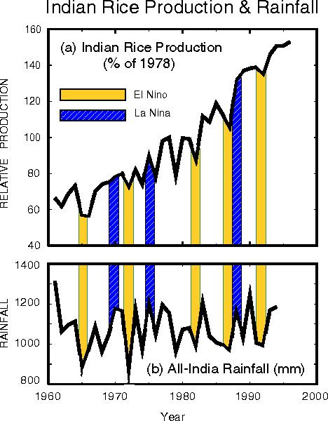
41 Figure 1. Example of the impact of large scale climate controls on the agriculture of a monsoon region. (a) Annual Indian rice production from 1960 through 1996 relative to 1978 (100 units). The shaded and dashed bars refer to Pacific Ocean El Nino and La Nina years, respectively. Rice shows a steady growth through the period but is marked by year-to-year deviations between %. (b) All-India Rainfall Index (AIRI) (in millimeters) defined by Mooley and Parthasarathy [1984] for the same period. Note that the variations in AIRI match the levels of rice production. (c) Detrended Indian rice production versus AIRI in terms of deviations from the mean. A moderately strong relationship (correlation 0.61) exists between the two indices, with El Nino seasons (solid triangles) corresponding to low yield and low rainfall. La Nina years (solid squares), on the other hand, are generally associated with high yield and high rainfall. (d) Relationship between the Southern Oscillation Index during the previous winter and the rainfall over India during the following summer. In general, Pacific Ocean warm events are associated with decreased precipitation over India while cold events are associated with enhanced rainfall. The variation of Indian rice production in time illustrates the points made in the last paragraph. Figure 1a plots the rice production in India between 1960 and Figure 1b plots the all-india rainfall index (AIR) (adapted from Mooley and Parthasarathy [1984]). The AIRI is a measure of the total summer rainfall over India. The relationship between crop yield and the AIRI was first noted by Parthasarathy et al. [1988] and extended by Gadgil [1996]. Figures 1a and 1b provide an updated version of this relationship. In general, rice production has increased linearly during the last few decades. Superimposed on this trend are variations in crop production of the order of %. Some periods of production deficit are associated with El Nino years in the Pacific Ocean (shaded bars) while some abundant years are associated with La Nina, or "cold" events in the Pacific (diagonal bars). Figure 1c is a scatterplot of the AIRI and crop production as functions of their percent deviations from the mean. The correlation between the two time series is All El Nino years (solid triangles) fall in the negative quadrant while all La Nina years (solid squares) lie in the positive quadrant. Finally, the relationship

42 between the preceding winter Southern Oscillation index (SOI) (the pressure difference between Tahiti and Darwin, e.g., Trenberth, [1975]) and the AIRI is plotted in Figure 1d. Generally, warm events in the tropics are associated with deficient rainfall while cold events appear related to abundant rainfall. The relationship between the state of El Nino-Southern Oscillation (ENSO) and the Indian rice yield suggest a number of questions. 1.Although the relationship between ENSO and Indian rice yield is not perfect, there is a tantalizing connection suggesting that the macroscale variations in the climate system influence variability on the scale of India and south Asia. How is this connection manifested in the physical system? 2.Does the relative vagueness of the ENSO and crop production relationship indicate that the intraseasonal variability of the rainfall within a particular summer relative to ploughing, planting, and harvesting (e.g., the timing of the onset of the monsoon and when the first break in the monsoon occurs) also has influence on the total crop yield? 3.Does the less than perfect relationship between the SOI and the AIRI suggest an inherent limitation to their linkage? If this is the case, what is the reason for this limitation? In the preceding discussion, Indian crop production has been used as an example of the importance of determining how climate variability on the macroscale influences the local scale. The questions raised above are common for the monsoon regions of Australia, Africa, and the Americas. 1.1.TOGA and Monsoons The Tropical Ocean-Global Atmosphere (TOGA) program was based on the assumption that the major climatic memory on the timescales of months to years is located in the tropical oceans. TOGA had the following very specific goals and scientific objectives World Climate Research Program (WCRP), [1985]: (1) gain a description of the tropical oceans and the global atmosphere as a time-dependent system in order to determine the extent to which the system is predictable on timescales of months to years and to understand the mechanisms and processes underlying its predictability; (2) study the feasibility of modeling the coupled ocean-atmosphere system for the purpose of predicting its variations on timescales of months to years; and (3) provide the scientific background for designing an observing and data transmission system for operational prediction, if this capability is demonstrated, by coupled ocean-atmosphere models. The extent to which these goals have been realized is discussed in National Research Council (NRC) [1996] To a large degree, emphasis within TOGA has been directed toward the physical processes occurring within the Pacific Ocean basin, a focus which has led to the identification of basic processes which control the longer-term aspects of the ENSO. Theories of ENSO fall into two basic classes: (1) the coupled system is a lagged oscillator [e.g., Anderson and McCreary, 1985, Schopf and Suarez, 1988; Cane and Zebiak, 1985; Battisti, 1988; McCreary and Anderson, 1991] or (2) the modulation is the result of unstable modes [e.g., Neelin, 1988; Battisti and Hirst, 1989]. The extent of our understanding of ENSO is illustrated by the moderately successful forecasts of the coupled ocean-atmosphere system in the Pacific Ocean [e.g., Zebiak and Cane, 1987; Cane et al., 1986; Latif and Graham, 1991]. So far, the models used in these endeavors have been relatively simple, and their success has allowed Cane [1991, p. 363] to make the following claim: The degree of forecasting skill obtained despite the crudeness of the model is telling. It suggests that the mechanism responsible for the generation of El Nino events and, by extension, the entire ENSO cycle, is large-scale, robust and simple: if it were complex, delicate or dependent on small scale details, this

43 model would not succeed. Many coupled ocean-atmosphere models show ENSO-like variations and support rational theories involving the joint interaction of the ocean and the atmosphere. There can be little doubt that the models do take into account fundamental physical processes. Figure 2. Annual cycle of outgoing longwave radiation (OLR) measured by satellite. Shaded and cross hatched regions indicate OLR < 220 and > 300 W m-2, respectively. OLR minima are surrogates for persistent deep convection and latent and radiative heat sources within the troposphere. Regions of maximum OLR, on the other hand, indicate radiative loss to space and hence are heat sinks. Figure 2 indicates an annual migration of the major atmospheric heat sources and sinks of the tropics and

44 subtropics. AfterWebster [1995]. Despite the importance of the ENSO phenomenon in climate variability on seasonal-to-interannual timescales, ENSO does not explain all of the variance. Furthermore, the forecasts of ENSO appear to have a distinct seasonality, such that error growth has a specific annual cycle [e.g., Webster and Yang, 1992; Webster, 1995; Balmaseda et al., 1995; Torrence and Webster, 1998]. Such variability may be caused by climatic features external to the Pacific basin. Although the heat source associated with the western Pacific warm pool is a critical element of the global climate and has a distinct influence on the global climate [e.g., Palmer and Mansfield, 1984], it is not the only region of intense atmospheric heating. This may be seen from Figure 2, which shows the annual cycle of outgoing longwave radiation (OLR) as determined from satellite. The shaded areas show OLR < 220 W m-2, which is considered to indicate convection and precipitation in the tropics [Arkin and Meisner, 1987]. There is a distinct migration of heating over south Asia during the spring and early summer. The heating variability is asymmetric with respect to the seasons with deeper convection extending considerably northward during the northern summer. During the southern summer the convection remains fairly close to the equator. This locus of heating is associated with the Asian-Australian monsoon system. Figure 2 also shows another interesting feature. OLR maxima (cross hatched regions) represent net radiative sinks. These heat sinks, principally associated with the deserts and the subtropical ocean regions, retain their geographic positions throughout the year. Since motions are driven by gradients of heating (i.e., the horizontal differences of heating between the heat sources and sinks) and not the absolute magnitudes of the sources and sinks themselves, the heat sinks are integral parts of the monsoon system. While the scientific objectives of TOGA have been partially accomplished by consideration of only the Pacific basin, it is clear that a thorough understanding of seasonal-to-interannual climate variability must take into account the monsoons. Earlier international field programs such as the Indian Ocean Expedition (INDEX) ( ) of the International Geophysical Year and the Monsoon Experiment (MONEX) ( ) [e.g., Krishnamurti, 1985] had made extensive measurements of the Indian ocean but not to the level of the TOGA investigation in the Pacific Ocean. These measurements were made against the knowledge that the monsoon also possesses interannual variability, some of which is linked to El Nino, although there seems to be inherent variance of the monsoon system itself or, at least, associated with other parts of the climate system. The picture that has emerged is a system that is global and interactive. Thus compartmentalization of the global system (i.e., the consideration of the ENSO and monsoon systems separately) is probably not very productive [Webster, 1995]. Most models used for experimental forecasting of seasonal-to- interannual variability [e.g., Cane, 1991] are essentially Pacific Ocean basin models. The models are "spun up" using observed Pacific Ocean wind distributions before the atmospheric model takes over and provides feedbacks to the ocean. Often, an annual cycle is added analytically to the system. However, the models appear to be very sensitive to any system or process that disturbs the wind strength over the Pacific Ocean of the model. For example, Barnett et al. [1989] found that weak trade winds, when imposed on an ocean model, produced a weak El Nino system. The weak trade winds introduced into the model were associated with a heavy winter snowfall regime and the subsequent weak summer monsoon. Matsumoto and Yamagata [1991], Webster [1995], Wainer [1991], and Wainer and Webster [1996], using models that include an Indian Ocean and an Asian landmass as well as a Pacific Ocean, found that variations in the intensity of the summer monsoon system affected the period of ENSO. Weak monsoons (and, consequently, weak Pacific trade winds) produced shorter period warm events. On the other hand, strong monsoons created longer-period ENSO cycles. Thus there appears to be some evidence that the coupled ocean-atmosphere response in

45 the Pacific Ocean is coupled strongly with events occurring outside the Pacific basin. Building on the foundations laid during TOGA, it is hoped to extend climate prediction from the Pacific basin to the global domain. It is planned to accomplish this extension under the auspices of a new program, Global Ocean-Atmosphere-Land System (GOALS) program [NRC, 1994; WCRP, 1995]. The aim is to expand the network of long-term observations and process studies to the other tropical oceans in order to encompass the major heat sources and sinks of the ocean-atmosphere-land system and investigate predictable elements that have been shown to exist in these regions. It is planned to follow the predictable elements found in the tropical coupled climate system to higher latitudes and, at the same time, seek predictable elements of the higher-latitude climate, if they exist. If there is inherent predictability at higher latitudes, it will most certainly be associated with oceanic dynamics or continental surface hydrological processes. Clearly, the GOALS endeavor will be a coupled oceanatmosphere enterprise but with the addition of land surface and ice processes all considered on a global domain. An important tool for GOALS is the global coupled ocean- atmosphere-land model. However, to date, there has not been universal success in simulating either the phase or the magnitude of the annual cycle with these models [Mechoso et al., 1995]. Perhaps part of the reason for these problems is the inability to simulate adequately even the mean state of the monsoon, which is a major component of the annual cycle even with stand-alone atmospheric general circulation models with imposed sea surface temperatures (SSTs) [Sperber and Palmer, 1996]. 1.2.Foundations Early studies considered the monsoon to be a regional physical entity, and attempts to understand its structure and variability focused naturally on local effects. As observations from farther afield became more readily available to researchers, indications emerged that the monsoon was a macroscale phenomenon which was intertwined and interactive with other global-scale circulations (see work by Kutzbach [1987] for a historical account of the south Asian monsoon). In recent decades, with the advent of a more homogeneous data set from satellites and a more substantial conventional database, there has been little to contradict this global view of the monsoon. Over 100 years ago, scientists attempted for the first time to forecast the seasonal and interannual variations of the mean monsoon patterns. The incentive to produce forecasts of Indian rainfall came after the great Indian drought and the resulting famine of As noted by Jagannathan [1960, p. 5], the charge from the Government Famine Commission to the director general of the Indian Meteorological Service, H. R. Blanford, was "so far as it may become possible, with the advance of knowledge, to form a forecast in the future, such aids should be made use of, though with due caution." In a first attempt to foreshadow the monsoon, Blanford [1884] considered the impact of local forcing functions such as the snow cover over the Himalayas during the previous winter. These efforts were eventually replaced by more global associations. Sir Gilbert Walker showed that the global atmosphere possesses coherent patterns of low-frequency variability (Walker [1923, 1924, 1928], Walker and Bliss [1932], corroborated by Troup [1965], Berlage [1966], and many others). Walker's [1923] work followed from the findings of a strong positive correlation between Russia and India by Blanford, [1880, 1884] and an equally negative relationship between Sydney and Buenos Aires [Hildebrandson, 1891]. Of the many planetary-scale interrelated patterns found by Walker [1924], the Southern Oscillation (SO) was thought to be of particular relevance to the monsoon and was described as "a swaying of pressure on a big scale backwards and forwards between the Pacific Ocean and the Indian Ocean." This definition was extended by Walker and Bliss [1932, p. 5] to include the seasonality of the oscillation: In general terms, when the

46 pressure is high in the Pacific Ocean, it tends to be low in the Indian Ocean from Africa to Australia; these conditions are associated with low temperatures in both these areas, and rainfall varies in the opposite direction to pressure. Conditions are related differently in winter and summer, and it is necessary to examine separately the seasons December to February and June to August. With the aid of such slowly varying circulations, there was hope that the variability of the Indian monsoon could be "foreshadowed" through relationships with other aspects of the general circulation, which Walker [1923, p. 320] termed "strategic points of world weather." Indeed, Walker's slow rhythms, most notably the SO, adumbrated the possibility of forecasting climate variations, which would be of singular importance to the agrarian society of India. Yet the ability to predict the future course of these rhythms was severely hampered by a vagueness in the observational relationships and by the failure to identify underlying physical processes which might have allowed the relationships to become unraveled. To make use of the observations of large-scale coherent rhythms for predicting the intensity of the subsequent monsoon, Walker would have had to satisfy four basic criteria [Webster and Yang, 1992]: (1) the precursor circulation (the SO) should possess a spatial scale which encompasses the circulation or the phenomenon (the monsoon) that is to be predicted; (2) the precursor should possess a timescale that is very much longer than that which is being predicted in order to provide sufficient lead time for the prediction to be useful; (3) the precursor circulation should be the "active" circulation and the circulation to be forecasted should be "passive." That is, an obvious cause and effect relationship should be apparent; and (4) the statistical relationships would need to be both stationary and significant.

47 Figure 3. Wavelet modulus analyses of climate time series in the Pacific ocean and the Indian Ocean. (a) Pacific Ocean sea surface temperature (SST) ( ) in the Nino 3 region (see Figure 14 for location), (b) The all-india rainfall index (AIRI) ( ), and (c) the cross-wavelet modulus between the AIRI and the SST. Contours indicate the percent of total variance at a particular frequency explained at a particular time in the data record. Thick black contours on each modulus indicate that the amplitude within is significant at the 95% level. The dashed areas on the right and left of the moduli distributions indicate the limitations of the data to define variance of a particular period at a particular time of the data record. Below each wavelet modulus is the data record, with a gray curve that represents the percent of the total variance explained at all frequencies at a particular time. The black curve below the crosswavelet modulus represents the covariance of the AIRI and the Nino 3 SST in the year-period band. On the right-hand side of each modulus are periodograms computed in two different ways. The gray curves represent the fast-fourier Transform of the

48 entire data series. The black curves represent the summed wavelet modulus. The 95% confidence curve is also plotted on the periodograms. After Torrence and Webster [1997] and Torrence and Compo [1997]. Figure 3 depicts relationships between the Nino 3 SST data (Figure 3a), the AIRI (Figure 3b) in the form of a wavelet analysis. Figure 3c shows the cross-wavelet modulus of the AIRI and the Nino 3 SST [Torrence and Webster, 1998]. A wavelet modulus provides a history of when in the data record certain periodicities are dominant and may be thought of as an evolving periodogram with time. Lau and Weng [1995] and Torrence and Compo [1998] provide excellent summaries of the use of wavelet analyses. The latter study is particularly useful as it provides a method of calculating significance levels of wavelet moduli. Significance levels at the 95% level are shown as the thick black contours. A crosswavelet analysis shows when certain periodicities were common to both data sets. Below each wavelet analysis is a plot of the time series (gray curve). The black curve represents the percentage of the total variance through the period of the analysis explained by the power at a particular time. On the righthand side of each wavelet analysis is a fast Fourier transform (FTT), or periodogram, of the data time series and the average wavelet modulus as a function of period. The FFT and the average wavelet modulus are very similar. The FFT provides the total power in a particular frequency band averaged over the entire data record. However, there is extra information in a wavelet analysis. If, during the data record, there was just one very large amplitude event at a particular frequency, the FFT may indicate large power but not disclose that it was the result of one event. The wavelet analysis, on the other hand, would localize the power in time and show that it was not a reoccurring phenomenon [Lau and Weng, 1995; Torrence and Compo, 1998]. With these thoughts in mind, the following conclusions can be drawn from the wavelet analysis. 1.The time series of SST in the western Pacific Ocean and the AIRI are not statistically stationary. There are at least three distinct regimes in which there were distinct and different periodic character to the series. Before 1920, there was considerable variance in the AIRI and the SOI, and correlations were near to between the AIRI and the SST compared to an average over the 120--year period of These high correlations early in the data period were the relationships that excited Walker and his colleagues. Between 1920 and 1960, there was little interannual variability in either the Pacific data or the Indian rainfall, and the correlation decreased to < Systematic analyses of the nonstationarity of the SOI was undertaken by Treloar and Grant [1953] and Grant [1953] for the Australian region and Troup [1965] for the globe. Correlations between Darwin surface pressure (a proxy for the SOI, see Trenberth [1984]) and also surface pressures in Hawaii with southern Australian rainfall anomalies decreased from roughly in the period to about between 1929 and Treloar and Grant [1953, p. 428] conclude that the secular reduction of correlations throws considerable doubt on the direct use of correlation relationships in forecasting.... Improvement in the performance of forecast formulae cannot be expected until there is a more satisfactory method of selecting indicators, requiring in turn a better understanding of the nature of weather processes. 2.The decrease in the correlations that occurred in the period between 1920 and 1960 has been replaced by an extended period of high variance in the SOI and correlations that match the period and a return of much higher correlations. These earlier studies were unaware that the ENSO signal possessed a large interdecadal signal. Both the SST and the AIRI moduli as well as the cross modulus show strong signals in the year period. Given the length of the data set, though, the conclusion should be viewed with some scepticism. However, recent coral core data from the Nino 3 region, which extents

49 back in time to 1600, exhibits similar variability in this period band (J. Cole, University of Colorado, personal communication, 1997). 3.Throughout the data period (except between 1920 and 1950), there is strong biennial monsoonal variance. A number of studies [e.g., Yasunari 1987, 1991; Rasmusson et al., 1990; Barnett, 1991] have commented on a biennial periodicity in tropical circulations, especially the monsoons. The periodograms indicate that the biennial variability is particularly strong in the monsoon regions, although with less magnitude in the SST fields. However, the cross modulus indicates substantial covariance in the year-period band. 4.The AIRI wavelet analysis shows substantial variance at intraseasonal timescales as well as clear interannual variability. Figure 4. Spatial distribution and seasonal cycle of the Darwin surface pressure for the period (a) Global distribution of the zero-lag correlation of surface pressure variations with the Darwin surface pressure. The distribution defines the Southern Oscillation index (SOI). The thick black contour denotes zero correlation, (b) Departure of the surface pressures (tenths of millibars) from the long-term boreal

50 summer mean value when the SOI is at 1 standard deviation (June-August). The thick black contour denotes the zero departure of Darwin pressure. (c) Boreal winter surface pressure departure when the SOI is at 1 standard deviation (December-February). Based on calculations bytroup [1965]. For the opposite extreme of the SOI, the sign of the pressure anomalies would be reversed. The thick black contour denotes the zero departure of Darwin pressure. Figure 4a depicts the spatial distribution of the zero--lag correlation of the Darwin surface pressure with surface pressure elsewhere [Trenberth, 1984]. It is now possible to return to the basic criteria (listed above) that Walker's [1923] indices would have to satisfy. The first two criteria are met. The pattern resembles a dipole with the extrema spanning the Indian and the Pacific Oceans. Furthermore, the general year period of ENSO is far greater than the intrinsic annual period of the monsoon. That is, the spatial and temporal scales of the SO easily encompass the scales of the monsoon. The third criterion proves much more difficult to satisfy. Walker [1923] found that Indian summer rainfall, while weakly correlated with pressure variations some months earlier in locations as far away as South America, was more strongly correlated with subsequent events. In discussing Walker's overall work Normand [1953, p. 469] summarized the following: To my mind, the most remarkable of Walker's results was his discovery of the control that the Southern Oscillation seemingly exerted upon subsequent events and in particular of the fact that the index of the Southern Oscillation as a whole for the summer quarter June-August, had a correlation coefficient of with the same index for the following winter quarter, though of only with the previous winter quarter. Thus Normand [1953, p. 469] could conclude with regard to the Indian summer monsoon that: It is quite in keeping with this that the Indian monsoon rainfall has its connections with later rather than earlier events.... Unfortunately for India, the Southern Oscillation in June-August, at the height of the monsoon, has many significant correlations with later events and relatively few with earlier events... The Indian monsoon therefore stands out as an active, not a passive feature in world weather, more efficient as a broadcasting tool than an event to be forecast.... On the whole, Walker's worldwide survey ended offering promise for the prediction of events in other regions rather than in India. There are numerous corollaries to Normand's conclusions. Contemporaneous relationships appear to exist between the AIRI and ENSO (see Figures 1 and 3), but a prior knowledge of the SOI in the previous winter or spring does not seem to help in forecasting the strength of the following summer monsoon. This is because of the lack of persistence of the SOI through the boreal spring. This persistence dip has been subsequently referred to as the "predictability barrier" by Webster and Yang [1992]. However, the persistence of the SOI for the 6-- to 9--month period following the boreal summer suggests that the winter monsoon and precipitation in Indonesia and north Australia is more highly predictable. Finally, the fourth criterion, the necessity for statistical stationarity of the SOI time series and its relationships with other indices, is questionable as first indicated by Troup [1965]. Troup [1965] described graphically why there are not clearer relationships between the SOI and Indian summer monsoon precipitation. Walker's [1923] correlations were reexamined by stratifying the deviations of surface pressure at the extremes of the Southern Oscillation from the long-term means by season. Planetary-scale regions of negative and positive sea level pressure are clearly evident in both

51 summer (Figure 4b) and winter (Figure 4c). However, in the boreal summer the zero anomaly line passes very close to the Indian subcontinent. That is, at the time of maximum precipitation in the annual cycle, India is located near a node in the pressure pattern and well away from the regions of anomaly extrema. While Troup's diagrams provide an explanation for the contemporaneous correlations of Indian rainfall and the SOI, they present a consistent picture of the vagueness of the relationship and why forecasting variations of the monsoon using just the SOI may be difficult. Small displacements of the node would place India in either a weak positive or weak negative pressure regime relative to the longterm summer average. Thus, even with a perfect forecast of the SOI, a discriminating foreshadowing of the summer monsoon over India would be rather difficult. On the other hand, the major precipitating regions of the winter monsoon occur well away from the nodes and near the extrema of the anomalies. Therefore, a priori, one may expect that forecasting the variability of the winter monsoon using the SOI might be more successful simply because the wintertime precipitation regions are located within a broad extremum of surface pressure and not near a node in the anomalous surface pressure field. Whereas research has concentrated on simultaneous relationships between the SOI and Indian summer rainfall [e.g., Angell, 1981; Rasmusson and Carpenter, 1983; Ropelewski and Halpert, 1987, 1989], many studies have persisted in attempting to use the SOI as a base predictor for monsoon variability, despite the conclusions reached by Normand [1953] and Troup[1965]. For example, Shukla and Paolino [1983] have suggested that the trend of the SOI in the preceding spring appears to be more important as an indicator of Indian monsoon precipitation than the absolute value of the SOI itself. However, lagged correlations between the trend in the SOI and the subsequent mean June to August (JJA) SOI are very weak and led Shukla [1987b, p. 540] to note that "the largest negative correlations are found in November following the monsoon season. This suggests a possible role of monsoon rainfall fluctuations.... in affecting the subsequent global circulation" tending to support the conclusions of Normand. Shukla and Mooley [1987] extended their analysis by configuring a regression equation comprised of the January to April Darwin pressure trend and the latitude of the 500--mbar ridge over the Indian subcontinent. In most studies the emphasis has been on the relationship of the Indian summer rainfall with gross-scale rhythms such as ENSO. Although there are critical socioeconomic concerns that have driven the regional emphasis, India represents only a moderate fraction of the monsoon area of Asia. It is not clear what the relationship is between rainfall on the Indian subcontinent and elsewhere in Asia, casting concern regarding the extent of the relationship between the gross external rhythms and the broad-scale monsoon. Thus it is important that some measure of the broad-scale monsoon intensity be defined. Besides relating monsoon variability with physical systems outside the monsoon regions, other relationships have been suggested. Noting that the monsoon anomalies appeared to run in multiple years (i.e., droughts tended to last for multiple years), it was suggested that sunspots determined monsoon variability. Blanford [1884], and later Lockyer [1904] found weak associations, but further scrutiny suggested phase problems. In the end it was concluded that sunspots merely enhanced the variability that was caused by other factors. Since then, however, interest has waned in the importance of sunspots in determining monsoon variability. As mentioned above, Blanford [1884] was the first to suggest that the intensity of the monsoon was governed by the extent of the previous winter snowfall over Eurasia. Early successes were replaced by failure [Kutzbach, 1987]. Hahn and Shukla [1976] suggested that Blanford's failure may have been a result of unreliable data and showed stronger relationships between snow extent and monsoon rain. Using more recent data, it was suggested that limited snowfall during the winter is associated with a stronger than average monsoon in the following summer. Excessive snowfall, on the other hand, was related to a weak monsoon. Dickson [1984] with a more extensive data set confirmed the analysis. Barnett [1984, 1985] and Barnett et al. [1989] noted that variability in the monsoons and the ENSO appeared to be related. A large-scale propagating surface pressure signal was observed to move through the Indian Ocean region into the Pacific Ocean with timescales greater than 2 years. The signal appeared to form in Asia, and Barnett [1985] suggested that it was associated with

52 Blanford's winter snowfall mechanism. With respect to gross-scale rhythms, Bjerknes [1969] made a key deduction which allowed a physical interpretation of the SO. Interannual variability, Bjerknes reasoned, was the result of interactive processes occurring between the tropical ocean and the atmosphere. Bjerknes was able to relate the quasi-periodic warmings of the Pacific Ocean (the El Nino) and Walker's [1923] SO, creating the concept of the ENSO phenomenon. Armed with Bjerknes's vital clue and with the realization that the long "memory" of the ocean might allow a predictive capability of the joint system, the international scientific community launched the TOGA monitoring and modeling program with the scientific objectives and goals listed previously Questions The discussion above may be summarized as a list of scientific questions relating to the structure of the monsoon itself, the relationship of the monsoon with other fundamental circulation features (such as ENSO), and the degree to which its low-frequency behavior can be predicted. The questions that will be tackled in this paper are the following. 1.What are the space and time characteristics of the monsoon system, and how do they relate to each other? The strongest signal of the monsoon is the annual cycle. Within the annual cycle there are active periods interspersed by lulls or breaks. What is the spatial scale of these intraseasonal events? Are they restricted to the south Asian monsoon, or do they occur in other monsoon regions as well? Monsoon seasons significantly different from the norm occur occasionally constituting strong and weak monsoons years. Is there a relationship between the number of active and break periods and the strength of the monsoon? Do the number of strong and weak monsoon years change from decade to decade? 2.What physical processes determine the structure and variability of the coupled ocean-atmosphere-land monsoon system? The physical processes that govern the coupled and variable ocean-atmosphere-land system are very complex. The monsoon may be thought of as the circulation responding to the annual cycle of solar heating in an interactive ocean-atmosphere-land system. Besides the interactive elements of the monsoon, there are influences from other climate systems such as ENSO and the extratropical regime. Figure 5. Possible relationships between the monsoon, ENSO, and other climate factors in terms of the complexity of interactions. In a "simple" system, changes in one system (e.g., ENSO; E) impart changes to another system (e.g., the Monsoon: M). Relative to the growth of internal errors (D) the influence is linear and the system highly predictable. In a "complex" system the relationship between the monsoon and ENSO is

53 complicated by interactions with other systems (C) which feed back onto ENSO, for example. The system is nonlinear, and the degree of determinism may be reduced depending upon the dominance of the link M to E (or vice versa). In a "tangled" hierarchial regime, determinism is lost. M, E and C may be unstable chaotic systems, and it is difficult to deconvolute linkages between the elements. Predictability of such a system would be entirely probabilistic. However, even with the tangled system, the degree of determinism would increase if one of the linkages were dominant. 3.What is the degree of complexity of the monsoon? A critical step toward determining a strategy for forecasting of the monsoon is to decipher its degree of complexity. Figure 5 shows three hierarchies of complexity following the concepts of Hofstader [1980]. The lowest form of complexity is a simple hierarchy, which states that the variability in a system (e.g., the monsoon, M) is forced by a variation in some other factor of the climate (e.g., ENSO, E). A second and higher form of complexity is a complex hierarchy where the two systems M and E are linked through other systems (Cn) such as middle latitude affects or Eurasian snowfall, for example. In turn, each connection may be influenced by nonlinear error growth (D). Within the complex hierarchy the monsoon may feed back on the ENSO system through the third system or vice versa. The highest level of complexity is a tangled hierarchy. At this level each system interacts with the other, and the routing of the interaction is difficult to decipher. It might be expected that there is considerable determinism in the simple hierarchy, although to a lesser degree in the complex hierarchy. In either of these complexities a particular precursor may lead to a specific conclusion, albeit blurred by nonlinear error growth in the system. However, determining the precursors and their order may be difficult in a multicomponent system. On the other hand, determinism would not be expected in the tangled hierarchy. The system would be highly nonlinear and chaotic, and predictability would be probabilistic. The principal purpose of this study is to provide a first step in producing a logical framework for determining the physical processes which control the seasonal-tointerannual variability of the coupled monsoon system and to provide a basis for future studies with coupled ocean-atmosphere-land models. This study attempts to form a bridge between TOGA, which gravitated to a Pacific Ocean basin focus, to the wider realm of the World Climate Research Program's (WCRP) GOALS project, which aims at seasonal-to-interannual prediction on a global scale. In the last two decades, there have been a number of reviews of the monsoon system [e.g., Ramage, 1971; Das, 1986; Fein and Stephens, 1987; Hastenrath, 1994]. This review differs by emphasizing the monsoon as a coupled system and, in the spirit of the Tropical Ocean Global Atmosphere (TOGA) program, emphasizes the predictability of the monsoon and its prediction. In the second section a thorough description of the monsoons is attempted. The processes that produce the monsoons are addressed in section 3. Modeling studies are discussed in section 4, and predictability and prediction of monsoon variability are discussed in section 5. Section 6 lists the main conclusions and discusses the transition of TOGA to GOALS.

54 3. Processes in the Monsoon Coupled System There are three fundamental driving mechanisms of the planetary-scale monsoon. These are (1) the differential heating of the land and the ocean and the resulting pressure gradient force between the differentially heated regions; (2) the impact of the rotation of the planet, relative to the orographic form of the lower boundary and the distribution of differential heating, which determines the character of the monsoon flow in both the atmosphere and the ocean; and (3) moist processes (in conjunction with rotational dynamics) that determine the strength, vigor, and the location of the major monsoon precipitation by storing, redistributing, and selectively releasing, in the vicinity of the summer hemisphere continents, the solar energy arriving over most of the tropics and subtropics. Although they are stated in simple form, each of these points represents an extremely complicated set of coupled processes existing between the atmosphere and the ocean and the atmosphere and the land. The complications arise because of the nature of the coupled system and render individual processes difficult to consider independently. To understand the monsoon system, it is necessary to deduce how the atmosphere, land, and ocean systems communicate. Communication occurs through the interfacial fluxes of heat, moisture, and momentum between the ocean, atmosphere, and land and the loss of heat to outer space. Modifications of the communications occur because of the impact orography has on the atmospheric circulation and coastline variations on oceanic dynamics Ocean-Atmosphere Interface It is apparent from Figure 10 that the SST in the warm pool region in the vicinity of south Asia and north Australia remain between C over most of the year. The warm pools are integral components of the El Nino-Southern Oscillation (ENSO) system and the planetary-scale monsoon systems of Asia, Africa, and Australia both in their mean form and in their interannual variability [Webster, 1987b]. Furthermore, small changes in the temperature of the warm pool have been shown to have major consequences on global climate [Palmer and Mansfield, 1984, 1986] and, as discussed in section 2, have a role in monsoon variability. For these reasons it is important to determine what controls the SST in the warm pools adjacent to the monsoon regions. There are three main oceanic regions that potentially influence the monsoon circulation. The first region is the warm pool of the western Pacific Ocean. In section 2, clear evidence of influences and connections between the strength of the Asian-Australian monsoon and the interannual variability of the tropical Pacific was established. The second region is the Indian Ocean. The Indian Ocean possesses a very strong annual cycle and an interannual variability which is somewhat smaller and usually in phase with the Pacific Ocean. The third oceanic region is the northwestern Pacific Ocean. Ju and Slingo [1995] have suggested that SST anomalies in the western and northwestern equatorial Pacific Ocean may be important in influencing the strength of the Asian summer monsoon. On occasion, these anomalies may be independent of ENSO. In the following paragraphs an attempt is made to understand the factors that control the SST in these three regions. The energy balance for a column of the tropical ocean mixed layer of temp

55 [e.g., Stevenson and Niiler, 1983] The net radiation R is made up of the net solar and longwave radiation (Snet+Inet) reaching the surface. Ft represents the sensible and latent heat fluxes out of the ocean through turbulent processes, and Fd represents the net export of heat out of the column by dynamic advection and entrainment through the sides and bottom of the ocean column. In addition, Fd takes into account the flux of radiant energy through the base of the mixed layer, which, under certain circumstances, can be important [Lewis et al., 1990]. H is the mixed layer depth, and Cw is the heat capacity of water. If the upper ocean is assumed to be well mixed, then its temperature T is a good approximation of the daily-averaged bulk SST. However, on the right-hand side, shortwave radiational heating generally varies only with cloudiness, as the surface albedo of the ocean is fairly constant. Longwave heating is more complex. The longwave radiational loss to the atmosphere increases with SST. The downwelling longwave radiation of the atmospheric boundary layer increases as well because of enhanced atmospheric water vapor loading and changes in atmospheric temperature. However, the changes in net longwave radiation in the tropical warm pools are quite small because of radiative saturation in the atmosphere near the ocean surface [Stephens and Webster, 1981; Ramanathan and Collins, 1991]. There are two components to the turbulent latent heat flux. For a given wind speed the latent heat flux, or evaporative cooling, increases with SST as the surface saturated vapor pressure is a function of SST only. On the other hand, the warm pools are generally regions of low wind speeds, so that the turbulent mixing tends to be minimized. It has been argued that the decreasing winds over the warm pools are the reason for the local latent heat flux minimum [Zhang et al., 1996]. Figure 24. Schematic of basic combinations of processes considered dominant in SST regulation. Balance 1 describes a local heat balance through thermodynamical factors. Balance 2 uses heat transports by the atmosphere in addition to local thermodynamical factors. Balance 3 utilizes ocean transports in concert (or independently with processes used in 1 and 2). Figure 24 shows a schematic of the basic combination of processes used in the studies of SST regulation

56 [e.g., McCreary et al., 1993; Godfrey et al., 1995; Loschnigg and Webster, 1996]. The first set is regulation through local thermodynamic adjustment. Such a state was defined by Ramanathan and Collins [1991] as the "natural thermostat" in which an SST warming produces cloud, which, in turn, reduces surface solar radiation flux and thus regulates SST. This is described in Figure 24 as "balance 1." The second set is regulation by a combination of atmospheric dynamics and transports in addition to negative radiational feedbacks. The invigorated atmospheric circulation responding to increased SST gradients enhances evaporative cooling of the ocean surface [Fu et al., 1992; Stephens and Slingo, 1992; Wallace, 1992; Hartmann and Michelson, 1993] (balances 2 and 1 in Figure 24). The third set is horizontal or vertical advection of heat or changes in the storage of heat by oceanic dynamics in addition to the first two sets. In this scheme the transport of heat by the ocean becomes iincreasing important (balances 1 through 3 in Figure 24). Determining the heat balances in the tropical oceans is difficult, and large differences may occur. Godfrey et al. [1995, p. 19] note that differences in estimates "should not be surprising as they are estimated as a relatively small sum of four quite large terms from empirical rules, and some of these rules are not very accurate." With some confidence, though, as a result of TOGA COARE, the surface heat flux into the western Pacific Ocean warm pool is estimated to be between 10 and 20 W m-2. However, this closure resulted from a major effort in the TOGA Coupled Ocean-Atmosphere Response Experiment (TOGA COARE) [Webster and Lukas, 1992; TOGA COARE, 1994]. Unfortunately, the heat balance is less well known in the Indian Ocean. Hastenrath and Lamb [1978], Hsiung et al. [1989], Oberhuber [1988], and Hastenrath and Greischar [1993] used climatological data to obtain estimates of net annual heat flux into the northern Indian Ocean between 50 and 70 W m--2. Despite uncertainties, it is clear that over the year there is a much stronger flux of heat into the north Indian Ocean than into the western Pacific Ocean. Furthermore, there is a far larger seasonality in this flux than in the western Pacific Ocean. The flux has maximum values in spring and early summer. Table 4 provides estimates of meteorological and upper ocean parameters for the north Indian Ocean and the western Pacific warm pool during the boreal spring and early summer using data from Oberhuber [1988] and TOGA COARE [1994], respectively. Both are light wind regions but with striking differences in the intensity of the solar radiation received at the ocean surface. The daily mean solar radiation into the north Indian Ocean is of order 250 W m--2 during the spring months compared to 150 W m--2 for the western Pacific, which accounts for the W m-2 imbalance in the north Indian Ocean. The main difference between the Pacific Ocean and the north Indian Ocean is that during spring and early summer the latter basin is devoid of highly reflective cloud, probably resulting from the very strong atmospheric subsidence. The subsidence arises from the proximity of desert regions which

57 surround the northern basin and the very strong convection occurring to the south of the equator. The very stable lower troposphere is not conducive to the formation of convection. Table 5 provides further details of the surface conditions over the north Indian Ocean (specifically the central Arabian Sea; 15N, 65E, and the central Bay of Bengal; 15N, 90E) before and during the established monsoon. The monsoon quickens later in the Arabian Sea than in the Bay of Bengal, which can be seen from the changes in the net radiation (high before the onset) and wind stress. In both locations the net heat flux into the ocean is strongly positive before the onset and negative after the onset. During the boreal spring and early summer the north Indian Ocean warms at a rate of just over 1C month from 27 to 30C. To test whether or not this warming is consistent with the net heating at the surface, a sophisticated one-dimensional mixed layer model [Kantha and Clayson, 1994] was forced by values listed in Table 4 for both the western Pacific and the Indian Oceans [Webster, 1994]. Estimates of the SST trends calculated from the model are shown in Table 4 and compared with observations. For the Pacific Ocean values the model suggests a small warming of about 0.5C month, which is more or less that which is observed during the boreal spring. However, north Indian Ocean values provide a warming of an isolated oceanic column of 3C month, which is a factor of 3 larger than observed. That is, if no other processes are taken into account, the north Indian Ocean should warm by between 9 and 12 C before the monsoon onset in May-June. Three immediate questions arise. 1. Why does the Indian Ocean warm at a rate that is much smaller than would be anticipated given the net heat flux into the ocean? The net flux of 100 W m--2 translates into a net heat gain of a petawatt (PW) over the north Indian Ocean basin. 2. What processes regulate SST in the Indian Ocean? Are they ostensibly different from other warm pool ocean regions? 3. How does the Indian Ocean transport its heat? It is clear that the hypothesis of Ramanathan and Collins [1991] cannot regulate the SST in the Indian Ocean. The warmest SSTs on the planet during spring and early summer are not associated with convection. Thus there is no cloud shielding to mitigate the solar radiation flux at the surface. In fact, the relationships between convection and SST are entirely different between the two ocean basins (Figure 25). Furthermore, the second class of theories for regulation of the SST in the Pacific Ocean [Fu et al., 1992; Stephens and Slingo, 1992; Wallace, 1992; Hartmann and Michelson, 1993] also cannot solve the

58 problem; winds remain light during the boreal spring and early summer, and evaporation is relatively low. Figure 25. Comparison of the OLR (W m-2, inverted scale) and SST (degrees Celsius) relationship between (a) the Indian Ocean and (b) the Pacific Ocean. OLR-SST pairs were computed from mean monthly data over the 11--year period ( ) in 2 by 2 longitude-latitude squares in the shaded regions shown in the maps below each panel. In the Pacific Ocean, there is a general increase in the height of convection (indicated by the reduced values of OLR) with increasing SST. At the warmest temperatures (> C), occurring mainly in the western Pacific Ocean there is a breakdown of this relationship. In the Indian Ocean, there is a sharply different distribution. No relationship appears to exist between SST and OLR at all. This lack of correlation suggests that deep convection results from other processes besides warm SST. Thus convection in the Indian Ocean may be more strongly tied to atmospheric dynamics than in the Pacific Ocean. There exists a common solution to all three questions. As summarized by Godfrey et al. [1995, p. 12]: on an annual average there is positive heat flux into the Indian Ocean, nearly everywhere north of 15S. The integral of the net heat influx into the Indian Ocean over the area north of 15S ranges between x 1015 W, depending on the climatology. Thus, on the annual mean, there must be a net inflow of cold water [into the North Indian Ocean], and a corresponding removal of warmed water, to carry this heat influx southward, out of the tropical Indian Ocean. That is, the SST is probably regulated by ocean dynamics. At the same time, the fact that SST and OLR are uncorrelated in the Indian Ocean suggests that convection is determined by processes other than ocean-atmosphere interaction in warm SST

59 regimes. One way to interpret the Indian Ocean OLR-SST relationship in Figure. 25 is that convection is determined principally by atmospheric dynamical processes or instabilities. To determine the importance of dynamical transports by the ocean, Loschnigg and Webster [1996] used the McCreary et al. [1993] dynamic upperocean model, which incorporates full upper ocean dynamics and thermodynamics. Although there is little subsurface data in the Indian Ocean, the model has been shown to replicate the surface structure of the Indian Ocean as well as its annual cycle [McCreary et al., 1993] when the ocean model is run in stand-alone mode with prescribed atmospheric forcing.

60 Figure 26. Results of the heat balance of the north Indian Ocean using themccreary et al. [1993] ocean model. (a) Time evolution of the oceanic heat flux across the equator into the north Indian Ocean. The transport refers to the heat flux across the equator (positive northward). Transport and storage values are the total of both model layers. (b) Seasonally averaged heat balance of the Indian Ocean basin north of the equator. Transport arrows indicate relative strength in each layer. Values given in Petawatts (1PW = 1015 W). After Loschnigg and Webster [1996]. Results are consistent with studies discussed in Godfrey et al. [1995]. Figure 26 shows the heat transport and heat storage changes in the Indian Ocean throughout the year. The instantaneous northward heat flux between two positions along a line of constant latitude is defined

61 as where Hi, Ti, and vi are the depth, temperature, and meridional velocity component of the ith layer of the model. The storage in a volume is defined by The major components of heat flow in this region are between the transport and storage terms. A very strong southward flux of heat is evident during the spring and early summer, and a reverse flux is evident during the winter, when the north Indian Ocean is losing considerable amounts of heat by evaporation and strong vertical wind mixing, which entrains colder water from below the thermocline. The net heat flux across the equator is made up of opposing flows in the upper and lower layer of the model and may be thought of as a seasonally reversing meridional ocean circulation [McCreary et al., 1993]. The magnitude of the net southward flux across the equator during the spring and summer months more than makes up for the excess surface flux into the north Indian Ocean, with peak summer magnitudes of meridional heat transport reaching values of PW. Whereas the changes in heat storage had been anticipated by earlier studies [e.g., Vonder Haar and Oort, 1973], the strong role of advection was not considered. The circulation found in the McCreary et al. [1993] model that accomplishes the cross-equatorial transport appears to have two major components: coastal upwelling along the coasts of the western Indian Ocean and Ekman transports. Wacongne and Pacanowski [1996] describe a process where the upwelled water within the western boundary currents are transported across the equator via the action of Ekman transports. Levitus [1987] was the first to note that meridional Ekman transports are southward in the Indian Ocean on both sides of the equator and in both the boreal summer and the annual mean. From the calculations above, it is clear that without ocean transport across the equator and changes in the heat storage of the north Indian Ocean, the cross-equatorial buoyancy gradient during early summer would be very large. Yet the processes that accomplish the cross-equatorial transport of heat in the ocean are essentially wind driven [Mohanty et al., 1996; McCreary et al., 1993; Godfrey et al., 1995]. In turn, the atmospheric circulation is driven by surface fluxes and heating gradients associated with the buoyancy gradient and atmosphere-land interaction. Therefore the annual cycle in the Indian Ocean is a coupled phenomenon resulting from ocean-land-atmosphere interactions and balanced, to a large extent, by cross-equatorial oceanic transports. While local heat balances and atmospheric heat balances are probably dominant in the western Pacific Ocean (i.e., balances 1 and 2 in Figure 24), dynamic transports of heat are still important [Sun and Liu, 1996]. However, the maintenance of SST anomalies in the northwestern tropical Pacific Ocean may be more strongly tied to ocean dynamics. For example, R. Lukas (University of Hawaii: personal communication, 1996) has noted that the Mindanao Current possesses interannual variability associated with the phases of ENSO. The Mindanao Current also appears to be tied to the strong flow from the Pacific and the Indian Ocean through the narrow channels between Borneo and New Guinea. This flow is termed the Indonesian throughflow [Gordon, 1986].

62 What is the role of the Indonesian throughflow in the annual heat balance of the Indian Ocean? Current measurements show [Fieux et al., 1996; Meyers, 1996] that the throughflow varies in magnitude on ENSO timescales between about 2 and 15 Sv. An assessment of the importance of the throughflow is given by Godfrey et al. [1995]. The water flux is from the western Pacific Ocean to the Indian Ocean. The Pacific warm pool thermocline is the deepest on the planet, so that the average temperature of the transported water into the Indian Ocean is about 18C. Topographic constraints suggest that this must return to the Pacific Ocean south of Australia [Hirst and Godfrey, 1993, 1995] but at a temperature of 6- -8C, so that, assuming a mean transport of 10 Sv, the throughflow provides about 0.5 PW to the Indian Ocean. From Figure 26 this number is comparable to the net surface flux over the northern Indian Ocean and a substantial fraction of the heat flux into the western Pacific warm pool. If these numbers are correct, it would appear that the Throughflow is an integral part of the heat balances of both the Pacific and Indian Oceans. Furthermore, as the variability of the Indonesian throughflow appears to be determined by the wind fields in the Pacific Ocean as they are modulated by ENSO, the export between the two basins would appear as an oceanic teleconnection on interannual timescales. From the discussion above, a further list of questions emerges: 1. Model results (see section 4) suggest that during periods of high ENSO variance (e.g., during the 1970s and 1980s) the SST anomalies in the Pacific Ocean are more important in perturbing the tropics than anomalies in the other ocean basins. The Indian Ocean anomalies appear to have less effect on the macroscale tropics. But do these SST anomalies play a role in the "fine structure" of the monsoon such as the timing of the onset or the frequency and occurrence of active and monsoon breaks? Also, what is the role of the Indian Ocean during periods when ENSO variance is small such as in the period ? At these times do the relatively small variations in Indian Ocean SST have a larger impact? 2. Does the Indian Ocean possess coupled ocean-atmosphere dynamics similar to the Pacific Ocean? El Nino like events have been observed in the Atlantic Ocean [e.g., Tomczak and Godfrey, 1994]. Do similar events appear in the Indian Ocean? There only appears to one report of a warm event in the Indian Ocean [Kapala et al., 1994] and with it anomalous rainfall in east Africa. During the summer of 1961 the seasonal ocean cooling in the western Indian Ocean was less than normal. At the same time, the SST in the eastern Indian Ocean was anomalously warm. Furthermore, there were anomalous surface easterly winds in the eastern Indian Ocean. There appears to be only two major impacts to these anomalous conditions in the Indian Ocean. The summer of 1961 was a heavy rain year for the Indian monsoon (see Table 3a). Also, the precipitation over east Africa for the period September-December was 4 standard deviations higher than normal. In terms of ENSO, 1961 was not an anomalous year. Whether or not ENSO-like events in the Indian Ocean have occurred at other times or whether the 1961 event was unique is not known. 3. The SST anomalies in the Indian and Pacific Oceans are generally in phase on interannual timescales. That is, during a Pacific Ocean warm event the north Indian Ocean also tends to be warmer than average. However, maximum transports via the throughflow occur during a cool event, so that if the throughflow is an important component of the Indian Ocean heat balance, there must be a lag. How is this lag manifested, and does it provide feedbacks which affect long-term ENSO variability? 3.2. Land-Atmosphere Interface In section 2 it was underscored that the monsoon cannot be understood in terms of the local thermodynamical processes associated with the precipitating areas of the monsoon. A fuller understanding comes from consideration of the heating gradients. Figure 9 showed that the monsoon consisted of both lateral and transverse monsoon circulations in addition to the Walker Circulation which must also be considered an integral component of the monsoon. Each of these branches is

63 associated with gradients of total heating with strong radiational and latent components. Furthermore, the rising parts of the circulations occur over the land surfaces of the pluvial regions of the monsoon (e.g., south Asia during summer) or the adjacent warm pools of the tropical oceans. The descending regions of the circulations occur over the ocean (see lateral monsoon component of Figure 9) or over the deserts (transverse component) and, in the early spring and summer in the north Indian Ocean, over very warm ocean surfaces Desert regions and the monsoon. The most permanent radiative sink to space is over north Africa throughout the year and over south Asia for all months except during the winter (Figure 2). Similar radiative sinks occur over the subtropical high-pressure regions. The persistence of the radiative loss and the existence of deserts are the results of a dynamic-radiational feedback process. Assuming that the atmosphere over a desert is dry, the heating of the surface radiates to space and is only minimally absorbed in the atmospheric column, and the downwelling infrared flux to the surface is thus reduced. Either the atmospheric column continually cools, or the heat deficit is made up of advection of heat from the surrounding regions or by subsidence. As the timescales of the change of the temperature structure of north Africa and the Middle East is roughly seasonal (i.e., determined by annual cycle of seasonal heating) and the radiative heat loss to space is of the order of 2--4C d--1 [Smith et al., 1982; Stephens and Webster, 1979, 1981], the heat loss must be balanced by the dynamic entrainment of heat [e.g., Webster, 1983b, 1987a, 1994; Ackerman and Cox, 1982; Blake et al., 1983; Rodwell and Hoskins, 1996]. This is manifested as strong subsidence over the desert region. The subsidence has two roles. First, the adiabatic warming of the subsiding air locally balances the diabatic heat loss. However, the descending air must be balanced by ascent somewhere else. Second, the subsiding air over the desert regions precludes the development of clouds by creating a stable environment and thus the reduction of radiative heat loss to space. This feedback renders the desert system climatically stable. This stability led Otterman [1974] and Charney [1975] to propose that the arid regions were self-perpetuating and that denudation of vegetation by overgrazing led to the extension of arid lands [see also Sud and Fennessy, 1982, 1984]. Figure 27. Schematic of the circulations between (a) the desert regions of north Africa and the Near East; and, (b) the subtropical ocean regions and the precipitating (pluvial) part of the monsoon circulation, respectively. The components of the monsoon match the transverse and lateral monsoon components shown in Figure 9. The dominant heating or cooling terms are shown in the boxes. "SH" and "LH" refer to sensible and latent heating. "RAD" and "EVAP" refer to radiational heating and evaporation, respectively. The pluses and minuses represent the signs of the processes and their relative intensity.

64 Figures 27a and 27 b show schematics of the circulations between the deserts and the subtropical oceans and the precipitating region of the monsoons. Also shown are the major heat sources and sinks associated with the components. Figure 27a is, in effect, a depiction of the processes involved in the transverse monsoon and the Walker Circulation of Figure 9. Figure 27b represents the lateral monsoon. The oceanic regions of radiative heat loss are collocated with the subtropical high pressure regions throughout the year. Maximum pressures occur in the high pressure regions of the winter hemisphere, however. On the other hand, with the advance of summer, the desert regions change from relatively high-pressure zones to local low-pressure regimes. Thus, the development of "heat lows" over the deserts seems to suggest that different processes are at play. The differences are due in part to the character of the surface fluxes that occur at the desert-atmosphere and ocean-atmosphere interfaces. Over the relatively cloudless desert regions, solar radiation heats the surface. This heat is dispersed in two ways: efficient radiation to space unimpeded by absorption by water vapor or cloud in the atmospheric column, and turbulent transfer of sensible heat to the atmosphere. However, Smith et al. [1982] point out that enhanced longwave warming takes place in the dusty region below the inversion. Thus the lower part of the atmosphere is heated by a strong diurnal component of sensible heating, plus absorption by dust, while the atmosphere above the dust layer cools to space. Turbulent transfer of heat upward may extend to 500 mbar at the height of summer. The result of the boundary layer heating is reduction of the mass in the column developing the heat low. The interception of the descending air from the large-scale inflow causes a very strong lower to middle tropospheric inversion. Over the ocean the radiative loss to space in the subtropics is less than over the desert regions because the SST is at a lower temperature than the continental surface and the boundary layer is moister. Sensible heat is relatively small, and the majority of the solar radiation is either mixed into the ocean or is used in the surface evaporation. This means that both the turbulent mixing and the local lower tropospheric heating is less over the ocean than over the desert. Furthermore, the mass of the column is diminished less, and the surface pressure remains as a relative maximum. The heat attained by the atmosphere from the ocean is in latent form and is not released locally but rather in the ITCZ region or over the continents. In this context the oceans may be thought of as a solar collector for remote regions where dynamical or mechanical constraints invoke vertical motion and the release of latent heat. During the winter the desert regions remain as net radiative sinks of the atmospheric column. However, the sensible heat flux to the atmosphere is less as solar radiation diminishes. The circulation becomes more similar to the oceanic case (Figure 27b) with the pressure increasing to become a relative maximum. The subsidence in the north Indian Ocean during spring and early summer appears to be a combined effect of the two sets of processes noted in Figures 27a and 27 b. The semi-enclosed ocean is surrounded by desert regions and may come under the influence of generally descending air as the continental regions heat. On the other hand, extremely strong convection occurs to the south of the equator [Tomas and Webster, 1997], and the north Indian Ocean may be under the influence of its subsidence as well. Further investigations will be required to test these hypotheses. A major conclusion that arises from this simple depiction is that the monsoons are integrated circulation systems which are indelibly tied to remote continental regions as well as the oceans. In the next section it will be argued that the local continental surface is also extremely important in determined the nature of the monsoon.

65 Moist land surfaces. In general, over the tropical and subtropical oceans, the Bowen ratio (the ration of sensible heat to latent heat flux) is very small. Latent heat fluxes are of the order of order 100 to 150 W m-2 compared to sensible heat fluxes of order 5 to 10 W m-2, giving a Bowen Ratio of between 0.1 to 0.05 [Hastenrath, 1987, 1994; Webster and Lukas, 1992; Webster, 1994]. Over desert regions the Bowen ratio may climb to 100 during the summer at the time of peak solar radiation. However, with the onset of the monsoon and with precipitation over land, the Bowen ratio in the continental regions may acquire values very similar to those over the ocean as latent heat fluxes increase. Thus local sources of water vapor are available over land as well as over the ocean and the sensible heat flux decreases with the lowering of the surface temperature of the wet land. Besides altering the ratio of sensible to latent heat, the albedo of the wet land decreases to values similar to those of the ocean surface. In addition, accompanying precipitation are changes in cloudiness and consequent alterations to the surface and columnar heat budgets. Overall, the moistening of the continental surface adds more degrees of freedom to the coupled structure of the monsoon. Prior to the onset of the monsoon, the system can be considered as principally an ocean-atmosphere system relative to a heated (and noninteractive) continent. Once precipitation occurs over land, the moist land surface processes require that the system be considered as a coupled ocean-atmosphere-land aggregation. Unlike the ocean, the supply of water over land is finite and depends on precipitation from the monsoon system. As the land dries out, the Bowen ratio as well as the disposition of radiation changes. Thus hydrological processes may impart a further intraseasonal variability on the monsoon system Snow cover. Many studies have found a statistical relationship between Eurasian snow cover in winter and Indian monsoon rainfall in the following summer [e.g., Hahn and Shukla, 1976; Dickson, 1984; Kripalani et al., 1996]. As Shukla [1987a] noted, an inverse relationship between Eurasian snow cover and the summer monsoon is not implausible because large and persistent winter snow cover over Eurasia can delay and weaken the spring and summer heating of the land masses that is necessary for the establishment of the large-scale monsoon flow. Persistence of snow also modulates surface albedo. During the spring and summer seasons following winters with excessive snow, solar energy which would be available to heat the surface is used for melting the snow or evaporating water from the wet soil. Yanai and Li [1994a, b, 1996] showed that there are three distinct peaks, near 36 and 2.25 years and 15 months in the power spectra of the monsoon intensity index defined by Webster and Yang [1992], the equatorial SST and the Eurasian snow cover. The quasi-biennial appearance of tropical variables such as sea level pressure (SLP), SST, and precipitation has been shown by many studies [e.g., Trenberth, 1975; Trenberth and Shea, 1987; Lau and Sheu, 1988; Rasmusson et al., 1990]. Barnett [1991] investigated the spatial distribution and evolution of variability of SST and SLP in the quasi-biennial and 37--year lowfrequency period ranges. The biennial tendency of the northern hemisphere snow cover has been pointed out by Iwasaki [1991]. The 15-month peak in the equatorial Pacific SST has been noted by Jiang et al. [1995]. Yanai and Li [1994b] investigated the phase relationship between the monsoon index, mean SST of various parts of the equatorial oceans, and Eurasian snow cover for the 36--year and quasi-biennial period ranges. For the quasi-biennial range the snow cover leads both SST and monsoon index. The phase relations for the 36--year period range are more complicated and suggestive of two-way interactions. More recently, Yang [1996] has suggested the existence of the inverse relationship between Eurasian winter snow cover and rainfall over India during the subsequent monsoon season. However, a precursor signal for Eurasian snowfall was found in the SOI, and evidence was found that the inverse relationship tends to break down during certain periods of ENSO. It was concluded that ENSO has a direct link on

66 the Eurasian winter snow cover. Within this scenario the snowfall over Eurasia is seen only as a link. Therefore the ultimate relationship exists between ENSO and the monsoon rather than between the snow cover and the monsoon. 3.3 Mechanical and Thermal Impacts of Orography The Asian-Australian region contains two orographic barriers that appear to have significant influence on the structure of atmospheric flow. These major barriers are the Himalayas-Tibetan Plateau complex and the east African mountains (Figure 11a). Both barriers appear to act as barriers to flow. There are also local mountain ranges such as the Ghats and the Burma (Myanmar) mountain range that cause major local variations to the monsoon. Although not evident in Figure 11a because of their spatial scale, the highlands of Indonesia and New Guinea are of considerable importance to the large-scale circulation of the tropics Himalayas and the Tibetan Plateau. The Tibetan Plateau extends over the latitude-longitude domain of E, N, with a mean elevation of more than 4000 m above sea level. Surface elevations change rapidly across the boundaries of the Plateau, especially the southern boundary. Strong contrast exists between the eastern and western parts of the Plateau in both landcover features and meteorological characteristics [e.g., Ye et al., 1979; Smith and Shi, 1995]. At these altitudes the mass of the atmosphere over the surface is only 60% that of sea level. Because of the lower atmospheric densities, various radiative processes over the Plateau, particularly in the boundary layer, are quite distinct and dominant compared to those over lower elevated regions [e.g., Liou and Zhou, 1987; Smith and Shi, 1992; Shi and Smith, 1992]. The importance of the Tibetan Plateau as an elevated heat source for the establishment and maintenance of the Asian summer monsoon circulation has been discussed by many authors (see, e.g., Ye et al. [1979], Gao et al., 1981; Murakami [1987a, b], He et al. [1987] and Yanai et al. [1992], for reviews). Flohn [1957] was first to suggest that the seasonal heating of the elevated surface of the Tibetan Plateau and the consequent reversal of the meridional temperature and pressure gradients south of the Plateau trigger the large-scale change of the general circulation over east Asia and the monsoon onset burst over the Indian subcontinent. To isolate the heating processes during the periods without appreciable rainfall and during periods affected by precipitation, Yanai and Li [1994a] examined the time series of the daily-averaged and vertically integrated heat source and moisture sink and the daily precipitation rate P for central and eastern regions of the Tibetan Plateau. The calculations for the two regions indicated that there were vast differences in the magnitude and timing of processes from one part of the Plateau to another. In the central Plateau, large values of appearing in May and early June were accompanied by insignificant values of and very little precipitation. In this region, significant amounts of precipitation occurred only after late June. Before the onset of the monsoon rains, large values of were noted. After the onset of rains the values of generally decreased, but the timing of peaks in the and series corresponded well to each other as well as to those in precipitation indicating contributions from the released latent heat of condensation. In the eastern Plateau, appreciable precipitation had occurred already in May. However, the values of were mostly negative in May, suggesting large evaporation exceeding precipitation. From June and onward, copious rains fell in this region, and the values and time variations of became similar to those of, showing that the release of latent heat of condensation was the dominant mechanism of heating over the eastern Plateau. During the winter (see Murakami [1987a] for a detailed review), the Himalayas-Tibetan Plateau complex acts as a major mechanical barrier to the extratropical westerlies producing strong stationary eddies in the seasonally averaged flow [e.g., Peixoto and Oort, 1992]. The mountains also modify the subseasonal timescale. To the east of the Himalayas, the steep terrain acts as

67 a natural duct for edge waves. These cold surges are dynamic manifestations of the outpourings of cold air from northeastern Asia as a combination of Kelvin and atmospheric shelf waves [Tilley, 1990; Compo et al., 1997]. Without the existence of the mountains the influx of cold air into the tropics would not penetrate as far south, would be farther to the east, and would be more modified by oceanic processes [Tilley, 1990]. Therefore during winter it is equally important to model the mountains with care and precision. This is underscored by Reynolds et al. [1994], who showed that the south Asia mountain ranges are a major source of internal error in numerical models. The dominating role of the Himalayas can be seen most simply by a comparison of summer monsoons of south Asia and north Australia. In the absence of a mountain range the precipitation over north Australia decreases linearly toward the center of Australia. Furthermore, the temperature anomaly over the Australian continent is far smaller than that associated with the summer monsoon (see Figure 6). Absent is the broad maximum of precipitation found over south Asia. Although it is difficult to compare the two monsoon systems (the sizes of the continents are different, and Australia is located nearer to the equator than south Asia), the similarity of the latitudinal precipitation distribution to that found by Hahn and Manabe [1975] in their nonmountain case is compelling. Although substantial progress has been made in understanding the role of the Tibetan Plateau in the Asian summer monsoon and the heating mechanism over the Plateau, many questions remain. 1. The relative significance of the sensible heat flux and the radiative flux [e.g., Smith and Shi, 1992, 1995; Shi and Smith, 1992] needs to be examined further. To understand fully the mechanism that carries sensible heat to the deep tropospheric layer during the dry pre-onset period will require direct measurements of convective elements in the boundary layer by remote sensing techniques. 2. Fu and Fletcher [1985] showed that the interannual variability of Indian monsoon rainfall was highly correlated with that of the thermal contrast between the Tibetan Plateau and the equatorial Pacific Ocean. Li and Yanai [1996] demonstrated that the timing and longitudinal extent of the reversal of the meridional temperature gradient south of the Tibetan Plateau vary year by year perhaps because of SST variations in the western Pacific Ocean [Fu and Fletcher, 1985]. However, the role played by the interannual variations of the surface and tropospheric temperatures over the Tibetan plateau in the variation of the Asian monsoon has not been studied systematically. 3.Although the strong diurnal variability of the moisture and heat fluxes must rectify to produce longerterm variability such as seen in Figure 3, the manner in which this rectification takes place is not clear. A detailed knowledge of these processes is important in determining how the diurnal variations is best parameterized in models The East African Highlands. The Findlater Jet (see Figs. 8 and 14) is an integral feature of the coupled ocean-atmosphere monsoon system. Besides being a critical element in driving the Somali Current [Knox, 1987] and thus being a key element in cross-equatorial ocean transports, the Findlater Jet is responsible for a large part of the atmospheric transport of water vapor across the equator. The jet is also an important component of the winter circulation, although at this time of year it is not as intense as during summer. The jet also exhibits variability on many timescales and is a keen reflector of the variability of the interhemispheric monsoon vortex and the active and break periods of the monsoon [e.g., Krishnamurti and Bhalme, 1976]. The strength of the Findlater Jet should have strong impacts on the ocean. A weak jet, for example, would be expected to alter the SST distribution of the north Indian Ocean by reducing upwelling, Ekman transport, and evaporation.

68 The early Findlater studies [Findlater, 1969a, b] were supplemented during the WCRP Summer Monsoon Experiment (MONEX, 1979). The location of the jet can be inferred from Figure 8 although the coarse scale of the contouring does not indicate its real intensity. The jet is centered around 1. 5 km and maximum core speeds of m s--1 extending from the northern tip of Madagascar to the central Arabian Sea. There have been many studies attempting to understand the physical processes that determine the location and structure of the Findlater Jet [Anderson, 1976; Hart, 1977; Bannon, 1979a, b; Krishnamurti and Wong, 1979]. The first four papers are theoretical studies that liken the jet stream to oceanic western boundary currents with the East African Highlands as the western boundary. Krishnamurti and Wong [1979] and Krishnamurti et al. [1990] modeled the baroclinic boundary layer of the western Indian Ocean driving a cross-equatorial flow against the model western boundary by an imposed vertically varying pressure gradient force. In each of the studies the structure of the jet stream is modeled fairly well. Perhaps the most important result of these studies is the setting of model vertical and horizontal resolution requirements for the adequate representation of cross-equatorial flow. If the scales are not fine enough, the cross-equatorial flow will not be concentrated in the western Indian Ocean but may spread across Africa and effectively disperse. Such was the case in early low-resolution general circulation experiments [e.g., Washington and Dagupatty, 1975]. In coupled ocean-atmosphere experiments a diminished Findlater Jet would be a critical omission as it would drive an inadequate Somalia Current and would probably lead to major changes in the heat balance of the north Indian Ocean. 3.4 Locations of Monsoon Convection The necessary but not sufficient rule of Riehl [1979] was that organized convection only takes place in the tropics when the SST is >27C. While the rule is generally true, Figures 8, 12, 15, and 25 indicate that the distribution of convection, especially in the monsoon regions, is far more complicated. However, it is possible to make some observations regarding where convection does occur and from this make a first attempt at determining processes. 1. The SST must be sufficiently warm (i.e., >27C) and the atmospheric structure so configured that the atmosphere is conditionally unstable. Thus very warm SSTs, such as those found in the north Indian Ocean, are not sufficient to produce convection because of the stabilizing effect of the large-scale subsidence. 2. In regions where there is a small or negligible cross-equatorial pressure gradient (e.g., the central Pacific during July in Figure 8) and where observation 1 is met, equatorial convection is found in the regions of warmest SST. In these regions the convection, warmest SST, and the low-level pressure trough are collocated. Such regions are the western Pacific Ocean in the boreal summer and the eastern Pacific Ocean in austral summer. 3. In regions where there exists a strong cross-equatorial pressure gradient such as in the African and American monsoon regions in the boreal summer, and the Indian Ocean in the boreal winter and the south Indian Ocean during the boreal winter and observation 1 is met, the organized convection is located in the summer hemisphere some from the equator (depending on the magnitude of the pressure gradient), usually on the equatorward side of the minimum sea level pressure and the maximum SST. 4. In regions of extremely strong cross-equatorial pressure gradient such as the Indian Ocean during the boreal summer, a hybrid state appears to exist. Observations 1--3 are evident, but low-frequency

69 variations of convection occur on the timescales of active and break periods and not on the shorter time scales noted in the regions with smaller cross-equatorial pressure gradients. Convection appears to locate near the equatorial trough or over the monsoon trough. Relative to observation 3, Tomas and Webster [1997] found signatures of inertial (symmetric) instability in the cross-equatorial flow, which were consistent with the ideas of Kuettner and Unninayer [1981] and Walliser and Somerville [1994]. The divergent component of the flow was a maximum at the line of zero potential vorticity (demarked as the thick contour in Figure 8). In regions of strong cross-equatorial pressure gradient the zero potential vorticity line lies some 3--7 poleward of the equator in the summer hemisphere. Divergence lies on the equatorial side of the zero line with convergence on the poleward side. Convection is collocated with the convergence. Furthermore, the rotational wind is a maximum to the north of the zero potential vorticity contour. Tomas and Webster [1997] argue that all of these features are consistent with inertial or symmetric instability. In regions of moderate cross-equatorial pressure gradient the convection appears constrained to one latitude belt. However, in the Indian Ocean in summer the convection appears to have two major locations and occasionally undergoes propagation poleward into each hemisphere. It is clear that the simple inertial instability arguments explain the disposition of convection during the Asian summer monsoon. Quite possibly, some type of hybrid dynamical instability exists in this complex state.

70 4. Monsoon Process Studies With Models Atmospheric general circulation models (GCMs) are well suited for the investigation of processes that determine the character of the monsoon. As the quality of GCMs improve, they are increasingly able to address the question of how regional climate, such as would be associated with monsoon rainfall and circulation anomalies, responds to imposed SST anomalies. At the same time, simpler mechanistic models and theoretical studies, especially used in tandem with GCMs, data analysis, and empirical and diagnostic studies, allow thoughtful investigations of particular processes and the testing of hypotheses. In the following paragraphs, examples of monsoon problems that have been successfully investigated using a broad range of models will be discussed Influence of SST Anomalies on the Monsoon Studying the impact of prescribed SST anomalies on the monsoon climate through coordinated atmospheric GCM integrations was one of the principal tasks of the TOGA Monsoon Numerical Experimentation Group (MONEG). As a focus of study, MONEG chose to investigate the monsoon seasons of June-July-August 1987 and As discussed in Krishnamurti et al. [1989a, b] these years were of particular interest for their contrasting behavior. On the one hand, 1987 was a severe drought year over both India and the African Sahel. On the other hand, 1988 was an above average monsoon season for India, while rains over the Sahel were close to their long-term climatological mean. In the first phase of coordinated experimentation, 17 atmospheric modeling groups ran 90-day integrations using the prescribed observed global SST fields for 1987 and 1988 as boundary forcing and atmospheric fields from operational numerical weather prediction analyses from June 1, 1987, and June 1, 1988, as initial conditions. These are referred to as the MONEG integrations; full results from these integrations are discussed WCRP [1992]. One of the major disruptions to the global climate during these years was associated with ENSO, which abruptly swung from a warm phase in the summer of 1987 to a cold event in The difference in SST between the summers of the El Nino year of 1987 and the La Nina year of 1988 provided 4C maxima in the eastern equatorial Pacific flanked by --1C values north and south of the equator. Other differences in SST are apparent around the globe, although they are much smaller in the Indian Ocean, which tends to be in phase with interannual variations in the central Pacific at least in the past few decades. The ability to simulate the basic monsoon climatology in a GCM is not a trivial matter, and many of the models contributing to the MONEG coordinated experimentation showed significant climate drift, often resulting in rather weak monsoon rainfall over some land areas (such as India).

71 Figure 28. June-August 200--mbar difference fields for (a, b) ECMWF analyses: (c, d) Monsoon Experimentation Group (MONEG) integrations (using ECMWF model with observed SSTs and observed initial states for 1988 and 1987: and (e, f) MONEG integrations with identical SSTs and initial conditions 1 day apart. Figures 28a, 28c, and 28e show velocity potential (contour interval 1x106 m2 s-1). Figures 28b, 28d, and 28f show stream function (contour interval 3x106 m2 s-1). From Palmer et al. [1992].

72 Figure 29. June-August 200--mbar differences between 90-day integration with observed SSTs from 1987 in specified region, climatological SSTs elsewhere, and 90-day control integration with climatological SSTs everywhere. The specified regions are (a, b) tropical Pacific, (c, d), Indian Ocean, (e, f) tropical Atlantic, and (g, h) extratropics. Diagnostics and contour interval are the same as Figure 28. FromPalmer et al. [1992]. Figures 28 and 29 show a fairly typical set of results from the set of MONEG-coordinated integrations using the ECMWF model [Palmer et al., 1992]. In Figures 28 and 29 the atmospheric circulation fields are shown in terms of 200 mbar velocity potential and stream function. These diagnostics give a "coarsegrained" measure of monsoon activity, and compared with more fine-scale structure over individual countries affected by the monsoons, most models in the MONEG set showed some skill in simulating to a large degree the observed interannual variability in these fields for 1987 and Figures 28a and 28b show the difference in velocity potential and stream function between 1988 and 1987 from ECMWF operational analyses. Figures 28c and 28d show the model-simulated fields. The pattern of enhanced upper divergence in 1988 over the Indian Ocean area (and reduced divergence over the Pacific) is fairly well simulated in the model, as is the reduction of upper tropospheric westerlies, particularly over South America, the Atlantic, and Africa. There are some discrepancies with the analyses, for example, in the stream function fields over the western Pacific. Whether these are associated with model errors or analysis errors is not known at present. Figures. 28e and 28f indicate, that, in terms of these coarse-grained diagnostics the atmosphere is not particularly sensitive to

73 atmospheric initial conditions. In particular, it shows that difference fields (based on coarse-grain diagnostics) between two integrations run with the same SSTs, but with different initial conditions (1 day apart), are very much smaller than the difference fields in Figures 28c and 28d. much smaller than the difference fields in Figures 28c and 28d. Overall, this model, typical of many within the MONEG experimentation set, was able to reproduce much of the observed coarse-grained interannual variability in the monsoon areas for 1987 and 1988, and the experimentation indicated that the level of skill was obtained through the underlying SST anomalies, rather than through the atmospheric initial conditions. This result is entirely consistent with the Charney and Shukla [1981] hypothesis that most macroscale variability in the tropics is determined by variations in the state of the boundary. It is important to assess which of the world's oceans contributed most to the simulated coarse-grained response (compare Figures 29c and 29d). Figure 29 shows the 200 mbar velocity potential and stream function difference between runs with observed SSTs (for 1987) in specified oceanic regions and climatological SSTs elsewhere and a run with climatological SST everywhere (the "control" integration). In Figures 29a and 29b the specified region where observed SSTs are used is the tropical Pacific Ocean; in Figure. 29c and 29d it is the tropical Indian Ocean; in Figures 29e and 29f it is the tropical Atlantic; and in Figures 29g and 29h it is the extratropical oceans. The results indicate that, overwhelmingly, the response shown in Figures 29c and 29d is associated with the observed SST differences in the tropical Pacific Ocean. Figure 29 does, in fact, show that the observed SST anomalies in the Indian and Atlantic Ocean do have some impact on the atmosphere over the Indian and Atlantic Oceans, respectively. However, it should be noted that the SST anomalies in these ocean basins have a substantial interdecadal component (i.e., the Indian and Atlantic Ocean SST anomalies in both 1987 and 1988 are not dissimilar to one another). On the basis of the results in work by Palmer et al. [1992], the response of the ECMWF model to Indian and Atlantic Ocean SST difference fields (between 1987 and 1988) was much weaker than the response forced by the Pacific Ocean SST anomalies. The role of interannual variability in the Indian Ocean on the Asian monsoon remains to be completely elucidated. However, the MONEG experimentation indicated that it is likely to be weaker than the remote effect of Pacific Ocean SSTs, at least during ENSO years and at least during the particular phase of the interdecadal variability of the period. Since the MONEG integrations were completed, Ju and Slingo [1995] have studied the role of Pacific Ocean SST anomalies on the Asian summer monsoon in more detail. These authors conclude that during La Nina years, warm SST anomalies in the tropical northwest Pacific may be of more direct importance in influencing the Asian summer monsoon than cold equatorial SST anomalies in the central and eastern Pacific. These results leave unanswered two basic questions: 1.What impact do the oceans have on the monsoon during other years in which ENSO is either absent or has a character different from the episode? 2.What is the impact of SST anomalies on more regional diagnostics such as country-wide seasonal mean rainfall. From a practical forecasting point of view these latter fine-grain monsoon diagnostics are obviously of more importance than upper tropospheric velocity potential Annual Cycle of Solar Heating of the Land and the Ocean The annual cycle of the solar forcing and the associated heating of the landmasses is generally considered to be the most important driving mechanism for the monsoon system. However, observations show that with the progression of the seasons, the regions of warmest SST in the Indian and Pacific

74 Oceans also advance northward. Does the annual march of SST also have a role in the establishment of the monsoon? To study this question, Shukla and Fennessy [1994] performed experiments with a GCM in which the solar forcing of the land and the ocean were incorporated separately. Three integrations were carried out, all of which were integrated through the boreal summer, ending on September 1. The control integration was initialized on January 1, 1987, and uses prescribed seasonally varying climatological SST and seasonally varying solar forcing. The fixed Sun (the "S" experiment) integration was initialized on March 1, 1987, and uses prescribed seasonally varying climatological SST, but the solar forcing was fixed at March 21 values throughout the course of the integration. The fixed SST ("SST") integration was initialized on March 1, 1987, and uses normal seasonally varying solar forcing, but the SST was fixed at March 1 climatological values through the course of the integration. Figure 30. Boreal summer (June-August) precipitation anomaly for (a) fixed Sun (S) and (b) fixed SST (SST) experiments. Contours are 1, 2, 4, 8, and 16 mm day-1. Dashed contours are negative, and areas below --2 mm d-1 are shaded. Integrations are made using the Center for Ocean-Land-Atmosphere Studies (COLA) model. From Shukla and Fennessy [1994]. The simulated anomalies (relative to the control integration) of the S and SST integrations were analyzed for the boreal summer period. The JJA mean precipitation anomaly for the S integration is

75 shown in Figure 30a, and the JJA mean precipitation anomaly for the SST integration is shown in Figure 30b. In both integrations, there is a dramatic reduction in the monsoon rainfall over the Arabian Sea, India, the Bay of Bengal, and southeast Asia. This reduction reaches a magnitude of 16 mm d-1 over Bangladesh in both integrations. There is also a nearly complete collapse of the monsoon flow and the Somali Jet for both the S and SST integrations (not shown). These results show clearly that the annual cycle of SST is crucially important for the establishment of the monsoon circulation and rainfall. This is particularly relevant for the modeling of the couple climate system. If a coupled ocean-atmosphere model is not capable of simulating the observed annual cycle of SST, the simulated monsoon circulation could be highly deficient Land Surface Processes There are two classes of candidate processes that have been proposed to explain why there are breaks in the monsoon. The first relates to influences from other locations on the monsoon region [e.g., Krishnamurti and Bhalme, 1976; Krishnamurti and Ardanuy, 1980; Yasunari, 1987]. The second set of theories [Webster, 1983a; Goswami and Shukla, 1984; and Srinivasan et al., 1993] describe the activebreak sequences as being internal oscillations of the monsoon system itself Moist processes. The impacts of the state of the continental surface have been studied through the use of GCMs. Many of these studies have concentrated on the west African Sahel following Charney [1975]. The impact of changes in albedo on precipitation was considered by Chervin [1979] and Sud and Fennessy [1982]. Their results tended to support Charney's hypothesis of an inverse correlation between albedo and rainfall. The impacts of soil moisture and vegetation have been investigated in a number of modeling studies [Walker and Rowntree, 1977; Shukla and Mintz, 1982; Sud and Fennessy, 1984; Xue and Shukla, 1993]. Xue et al. [1994] considered the impact of ground moisture on the state of the Indian monsoon. These studies draw one common conclusion. The surface characteristics of the continental landmasses were of great importance in determining the structure of the monsoons, and there was particular sensitivity to soil moisture. That is, soil moisture is an active component in the evolution of the monsoon system and a component that requires careful modeling. Webster and Chou [1980b] suggested that moist land-surface processes could introduce feedbacks resulting in intraseasonal monsoon variability. Models simpler than GCMs were used to study complex processes involved in the interplay between moist surface hydrological processes and the monsoon circulation. For example, Webster [1983a], Srinivasan et al. [1993], and Dixit [1994] used a simple zonally symmetric atmospheric model coupled to a mixed layer ocean and a simple surface hydrological system. The hypothesis originally tested by Webster [1983a] was that the interplay between ground hydrology and the atmospheric circulation did not allow the system to reach an equilibrium and that the northward propagations of convection of the order of day period noted in Figure 15 were the result of this instability. Similar results were found by Nanjundiah et al., [1992], using the same model. The reason for propagation of convective zones with interactive surface hydrology may be seen rather simply by considering the first law of thermodynamics

76 where T is the temperature, w is the vertical velocity (dp/dt), S is a measure of the static stability, and Q dot is the diabatic heating rate in the column. If the system is in steady state then the diabatic heating or cooling must be balanced at all locations by adiabatic processes (i.e., ws = Qdot ). Such would be the case if the system were simply driven by the release of latent heat in the column. The location of the vertical motion maximum will be a function of the variation of solar heating unless dynamics (e.g., instabilities) or surface characteristics do not feed back to force Q dot and the vertical velocity field to become out of phase. Thus, over the ocean, where the thermal inertia is large, the location of convection should be slowly varying. Over land, where surface characteristics may vary more quickly than over the ocean, equally rapid changes in the surface heat fluxes can occur with ensuing changes in convection. The heat balance at the continental surface is made up by a combination of net radiative heating and the turbulent fluxes of sensible and latent heat. Before convection occurs, solar radiative heating dominates, and the Bowen ration is large. Once convection commences (e.g., near the coast), precipitation produces changes in the moisture balance at the surface. The Bowen ratio, initially very high, drops appreciably in the vicinity of convection. Likewise, the solar radiation reaching the surface decreases as well (because of associated cloudiness increases), decreasing the surface heating and the sensible heat flux into the column. To the north, the solar heating remains large, and the sensible heating of the atmosphere continues. That is, poleward of the convection, the Bowen ratio continues to be high. As a result of the heating and the vertical velocity becoming out of phase, the region of continental convection will move northward. In summary, these changes in the continental surface heat budget were used to explain the northward propagation of convection first noted by Sikka and Gadgil [1980]. The basic timescales of the propagations of the convection are set by the surface recovery time [Webster, 1983; Goswami and Shukla, 1984; Srinivasan et al., 1993] Influence of snow cover. Anomalous land surface conditions (e.g., snow cover and soil moisture) appear to influence the seasonal land-ocean differential heating, and possibly influence the Asian summer monsoon system (e.g., Hahn and Shukla [1976], Dickson, [1984], and many others). Modeling studies [Barnett et al., 1989; Yasunari et al., 1991; Vernekar et al., 1995] demonstrated that albedo and hydrological effects of snow cover may be responsible for the anomalous seasonal heating of the atmosphere. Barnett et al. [1989] suggested that the anomalous excessive snow cover over Eurasia may trigger ENSO-like conditions in the equatorial Pacific by means of a weakened summer monsoon and intensified equatorial westerlies. The SST field in the model developed a weak El Nino structure in the equatorial Pacific. Their results demonstrate the importance of land processes in global climate dynamics and their possible role as one of the factors that could trigger ENSO events. Yasunari and Seki [1992] found significant time-lag relations between Eurasian snow cover in boreal spring (April), the Indian summer monsoon rainfall, and the SSTs in the equatorial western Pacific in the succeeding winter. The seasonal hemispheric circulation anomalies composited for strong (weak) Indian monsoon years show anomalous stationary wave patterns in the extratropics that may be forced by the anomalous coupled monsoon system in autumn to winter. This, in turn, may feed back to produce a more (less) extensive snow cover anomaly over Eurasia leading to the weak (strong) monsoon for the following summer. Webster and Yang [1992] found large-scale circulation patterns that were precursors to strong and weak monsoons. These patterns, which persisted through the winter prior to the anomalous monsoon, may be consistent with the circulation patterns of Yasunari and Seki [1992]. Using results from a 70--year integration of coupled ocean-atmosphere general circulation model experiments, Meehl [1994b] demonstrated a very similar biennial cycle of the coupled monsoon system in concert with the extratropical flow regimes. In this biennial cycle the combined effect of anomalous

77 convection over the Asian monsoon and African monsoon is stressed as important for producing the circulation anomalies in the extratropics (Figure 31). Meehl [1994b] also suggested that cold air advection (and the subsequently cooled surface) prevailing over the Eurasian continent in winter may be more important than the effect of anomalous snow cover itself for producing anomalous monsoon and convection in later seasons. Figure 31. Schematic evolution of the biennial component of the monsoon circulation from (a) the winter before a strong Asian monsoon through (b) the strong monsoon season to (c) the northern winter after the strong monsoon before a weak monsoon, to (d) the following weak monsoon. FromMeehl [1994]. Yasunari [1989] noted a role for the east Asian winter monsoon in the global-scale TBO through strong negative correlation between the Indian summer monsoon and the following SST anomaly in the South China Sea. They argue that the SST anomaly is indicative of strength of the east Asian winter monsoon surge. That is, a stronger south Asian summer monsoon is likely to produce a stronger east Asian winter monsoon and vice versa, presumably through some form of atmospheric teleconnections [Yasunari and Seki, 1992] and associated land surface processes (e.g., snow cover) over the Eurasian continent. The SST anomaly in the south China Sea thus produced in winter, and persisting through the following spring and early summer, may initiate reversed anomalies of convective activity in the equatorial western Pacific. This surmise is corroborated by Matsumoto and Yamagata [1991], who found that the windstress associated with surges in the winter monsoon is consistent with changes in the western Pacific SST between winter and the following boreal summer.

78 4.4. Monsoon and Orography Several numerical [e.g., Hahn and Manabe, 1975; Kuo and Qian, 1981, 1982; Chen and Dell'Osso, 1986; Kitoh and Tokioka, 1987; WCRP, 1992] as well as laboratory experiments (Ye et al., 1974; Chen and Li, 1982) were performed to clarify the thermal and orographic effects of the Tibetan Plateau in determining the characteristics of the monsoon. The overall importance of the orography on the monsoon has been demonstrated by Fennessy et al. [1994] who found that replacement of an enhanced silhouette orography by a mean orography was more representative of actual barrier heights. This formulation of orography produced a more realistic simulation of monsoon rainfall. In addition, a series of numerical experiments in which large-scale uplifts of the Tibetan Plateau were linked to the climatic changes on the geological timescale elucidated the effects of the Plateau on the planetary-scale circulations [Kutzbach et al., 1989; Manabe and Broccoli, 1990]. Beyond isolating important physical processes and illustrating the role of the Himalayas-Tibetan Plateau as a major modifier of the northern summer monsoon system, Hahn and Manabe [1975] and others established that general circulation and prediction models must contain a careful configuration of orography. With the advent of coupled models, the configuration will have to be even more precise. The Himalayas are also the source regions of the major river systems of south Asia, which are, in turn, responsible for the flux of fresh water into the north Indian Ocean [e.g., Knox, 1987; Tomczak and Godfrey, 1994] and the stabilization of the upper ocean, particularly in the Bay of Bengal. The modeling of the mountain ranges, their influence on the water balance, and the subsequent role in the salt budget of the oceans is a major challenge for the future. 4.5.Influence of the Monsoon on ENSO, Numerous studies have been used to test the conclusion of Normand [1953] that anomalies in the monsoon influence the amplitude and phase of ENSO. To date, these experiments have been performed using simple models in contrast to the reverse experiments (the influence of ENSO on the monsoon), which have utilized full atmosphere GCMs. The latter experiments were described in section 4.1. Matsumato and Yamagata [1991] modeled the origin of ENSO in the Pacific Ocean and the role of monsoon forcing on ENSO. Webster [1995] and Wainer and Webster [1996] used a simple coupled ocean-atmosphere model with a Pacific Ocean and an Indian Ocean surrounded by an "African" and an "Asian" continent. The Pacific Ocean and the Indian Ocean were separated by a thin impermeable wall (Figure 32a). The model, driven only by the annual cycle of the Sun, exhibited interannual variability which with standard parameters exhibited a period of about 4 years. The amplitude of the monsoon heating was parameterized so that it was possible to alter its phase and magnitude. The model ENSO proved to be very sensitive to the strength of the monsoon forcing. Values chosen for the experiment matched estimates of monsoonal heating determined from observations [Wainer and Webster, 1996].

79 Figure 32. Coupled ocean-atmosphere model indicating that the monsoon can alter the period of warm events in the Pacific Ocean. (a) The model domain which consist of an Indian Ocean, separated from a Pacific Ocean and surrounded by an Asian and African Continent. The ocean model is themccreary and Anderson [1991] 1 1/2 layer model and the atmosphere is a free surface barotropic model. The coupled system is driven by an annual cycle of heating. (b) The response of the model Nino 3 region for strong, standard and weak monsoon heating over land during years 30 through 60 of the integration. As the amplitude of the monsoonal heating increases, the period of the ENSO cycle increases. (c) The response of the model Nino 3 region to stochastic forcing

80 of the monsoon. The SST response shows a more chaotic structure. Results are from Wainer and Webster [1996]. Figure 32b shows that as the monsoon forcing becomes stronger, the period of ENSO becomes longer. On the other hand, relative to weak monsoon forcing, the ENSO period shortened. Finally, a stochastic forcing was developed with characteristics that matched the observed variability of the monsoon. Figure 32c shows the impact of the stochastic period. The model ENSO possesses an average period similar to that with the unperturbed monsoon forcing. However, the response is also chaotic with periods in between warm events as short as 4 years and as long as 10 years. Within the context of an extremely simple surrogate of the natural system, it would appear that the strength of the monsoon plays an important role in ENSO, at least as a perturbing factor. It should be borne in mind, however, that the full cycle of interaction was not allowed in these integrations, and the modified ENSO cycle in the model did not feed back to alter the monsoonal heating Modeling Issues The ability of a model to investigate processes depends very much on the ability of the model to simulate realistically the mean climatology. The old quasi-linear paradigm was that the simulation of a mean climatology was largely irrelevant as model errors were systematic and would be subtracted out when anomaly fields (i.e., difference between perturbed states and the control integrations) were computed. However, in the calculation of the difference between 1987 and 1988, two seasons of great differences in rainfall over India and extremes in the SOI, Shukla and Fennessy [1994] amply demonstrated that the state of the basic model was of paramount importance. The current Center for Ocean, Land and Atmosphere (COLA) GCM was used to test the Charney and Shukla [1981] hypothesis (subsequently supported by Palmer et al. [1992] and Mo [1992]) that the state of the lower boundary condition strongly influenced the monsoon. Even with the observed SST with the El Nino in 1987 and an La Nina in 1988, the old model was not able to simulate two of the largest extreme years of Indian rainfall. Furthermore, the difference of the two simulations did not bear close resemblance to the observed precipitation differences. Thus, either the hypothesis failed, or the base model was inadequate. With an updated version of the model, which included better representation of orography and changes in the handling of soil wetness, vegetation, and cloudiness, both the simulations of the individual seasons and the differences of the seasons were well simulated. Similar improvements in the ability of the ECMWF model to simulate monsoonal and tropical rainfall occurred with changes in the latent heating algorithm [Miller et al., 1992]. The second phase of the MONEG project involved the analysis of monsoon activity in the set of 10-year integrations that constitute the Atmospheric Model Intercomparison Project (AMIP) [Gates, 1992]. These models were integrated with identical SSTs (derived from observations over the decade ). Under the TOGA MONEG project a monsoon diagnostic component of AMIP was established. The results from this component are summarized below. A more extensive analysis is given by Sperber and Palmer [1996]. As was found from the earlier 90-day coordinated MONEG integrations, the ability of GCMs to simulate satisfactorily the observed correlation between interannual monsoon and SST variability was associated with the skill in simulating the mean monsoon. In these integrations none of the models were able to reproduce the observed empirical relationship between ENSO and the south Asian monsoon.

81 In the AMIP analysis both coarse- and fine-grained measures of monsoon activity were diagnosed. One coarse-grained measure was the wind shear index of Webster and Yang [1992], which can broadly be thought of as corresponding to the scale of variation discussed above for the velocity potential and stream function maps in Figs. 28 and 29. Rainfall variations on the national-scale regions were taken as measures of fine-grain monsoon activity. The AMIP integrations were used to measure skill in simulating fine-grain structure of the monsoon. The measure calculated was the evolving AIRI during the integration period. Extremely large scatter was found between the 33 AMIP models (see Figure 32). Even when the models were quality controlled by eliminating those models that failed to model adequately the long-term mean Indian rainfall distribution, the spread was still very large. An important question arises; what is the origin of the spread between the models? For example, if a single model were integrated from different initial conditions, would the same level of intraensemble spread be apparent, or does the level of spread reflect model-formulation differences only. After all, the Indian Ocean region is extremely complex (see Figure 11a), and large- scale orography has been shown to be a major source of internal error [Reynolds et al., 1994]. To quantify this question, the ECMWF model was run in ensemble mode and six realizations of AIRI computed (Figure 32c). The spread between the realizations was less than the spread between the "quality- controlled" models. Thus some part of the spread in the AMIP integrations is due to model formulation differences. However, it remains to be determined with several state-of-the-art GCMs, whether the intraensemble spread between the members is comparable to the signal arising from the SSTs. This suggests that there is an intrinsically unpredictable component to the seasonal AIRI predictability associated with sensitivity to initial conditions.

82 Figure 33.Atmospheric Model Intercomparison Project (AMIP) integrations for the Indian region. (a) The Indian rainfall simulations of the 32 AMIP models to identical SST variations over a 10-year period. Figure 33a (bottom) shows the response of an ensemble of ECMWF model integrations with perturbed initial conditions. (b) The same as Figure 33a, except for the Sahel region. The ECMWF ensemble shows greater coherence in the Sahel integrations than the ensemble for the Indian case. On the other hand, the reproducibility of the AIRI in the AMIP integrations should be contrasted with that of coarse-grained measures of monsoon activity. For example, for the ECMWF model, the reproducibility of the Webster and Yang [1992] windshear index is well over 3 times larger than it is for the AIRI. In some sense it could be argued that it is inevitable that smaller reproducibility will be associated with small-scale features. However, this is not entirely straightforward. According to results by Sperber and Palmer [1996] the reproducibility for the March to May Brazilian Nordeste, the Sahel, and over the tropical Pacific warm pool rainfall was much smaller (Figure 33) Thus the AMIP results suggest that there is something intrinsically less predictable about aspects of the regional seasonal-mean rainfall associated with the Asian summer monsoon than the regional seasonal- mean rainfall in other parts of the world which is not associated simply with spatial scale. It could be argued that the differential spread of the ensemble members can be explained through the hypothesis that the dynamics of intraseasonal variability in the Asian monsoon area is intrinsically chaotic and that nonlinear coupling between the intraseasonal and interannual timescales makes the fine-grain seasonal-mean monsoon

83 diagnostics only partially predictable. These ideas will be weighed against other possibilities and critically evaluated in the next section.

84 5. Predictability and Prediction of the Monsoon Hastenrath [1994] listed five main approaches in climate prediction: (1) the extrapolation of presumed periodicities existing within a data record, (2) the assessment of statistical relationships between local phenomena of interest (e.g., rainfall, pressure) and data at some distant phenomenon, (3) the relationship of the local precipitation prior to the rainy season with precipitation at the peak of the rainy season, (4) comprehensive diagnostic and empirical studies of climate and circulation anomalies combined with statistical analysis, and (5) numerical modeling. In this section we review the current understanding of the predictability of the space-time averaged monsoon circulation on seasonal-to-interannual timescales with particular emphasis on approaches (4) and (5). At the same time, speculations will be made on emerging ideas of monsoon predictability that were mentioned in section The Basic Question of the Predictability of Monsoons In a review article on the interannual variability of the Indian monsoon, Shukla [1987a] posed two questions. Even though they pertain to one region within a much larger-scale phenomenon, they are of enough importance be repeated here 1.Is the behavior of the seasonal mean monsoon primarily determined by a statistical average of a variety of independent short-period fluctuations that are not related to any seasonal or other lowfrequency forcing? 2. Are there global- and planetary-scale "forcing functions" (either due to slowly varying boundary conditions at the Earth's surface or due to very low frequency changes like the Southern Oscillation) that determine the interannual behavior of the seasonal mean monsoon circulation and rainfall, and is the interannual variability of the short period fluctuations controlled by such large-scale low-frequency forcing? To these two questions a third may be added 3.Are there low-frequency hydrodynamical instabilities of the monsoon circulations themselves that, on the one hand, exert control on the short-term fluctuations described in question 1 and are, in turn, modified by the large-scale planetary controls described in question 2? These questions are important as they define the basic essence of the predictability of monsoon variability The degree to which monsoons are predictable depends upon the space scale and timescale for which predictability is being sought. The day-to- day changes in rainfall at any place are determined by the life cycle of synoptic scale disturbances (lows, depressions, monsoon trough, etc.) at or around the place of consideration. Thus predictability of day-to-day weather at a point in the monsoon region is in no way different from that of any other point on the globe and is limited to a few day

85 the monsoon was controlled by processes described in question 1, then there would be no greater predictability for the monsoons than would be expected for the extratropics. On the other hand, if the monsoon were controlled solely by large-scale evolving processes as discussed in question 2, one would expect that the limits of monsoon prediction would be given by the limits of predictability of the planetary-scale forcing functions. However, if there were large-scale and low-frequency instabilities of the monsoon which might, for example, determine the intraseasonal active and break periods of the monsoon, then one may expect hybrid limitations to predictability existing somewhere between question 1 and question 2. These concepts are discussed in the following paragraphs. There is some disagreement about the degree of predictability of the monsoons or whether they are predictable at all. There are, in fact, two vastly differing schools of thought. One hypothesis is that the variations of low latitude phenomena including the monsoons are the results of influences from slowly varying boundary conditions. For example, Charney and Shukla, [1981, p. 107] state there is : evidence from numerical experiments and from observations that natural fluctuations of short period [less than seasonal] are adequate to account for most of the observed variability at midlatitudes, but are not capable of explaining the variability at low latitudes, say below 30N. In addition... numerical and simulation experiments and statistical analyses of observations that anomalies in sea-surface temperature and in ground albedo are capable of producing large variances. Since these anomalies are usually of long duration, the possibility arises that mean monthly conditions at low latitudes, such as monsoon rainfall, may be predictable with some accuracy.... Thus we suggest that the synoptic-scale flow instabilities which limit prediction so drastically at midlatitudes have less influence at low latitudes and therefore leave room for longer-period and more predictable signals to make themselves felt. The basis of this thesis is that since the large-scale tropical atmosphere is not as generically hydrodynamically unstable as is the extratropics, then the response of the large-scale tropical circulation to underlying lower-boundary anomalies should, compared with the extratropics, be more reproducible and hence predictable. This central concept expressed in Charney and Shukla, [1981] formed the basis for TOGA. At the other end of the spectrum are those who believe that the monsoon system is chaotic and that generalities about the monsoon, upon which prediction would depend, cannot be made. For example, Ramage [1971, pp ] states that from the earliest days of monsoon research in Asia, meteorologists have constantly tried to find order in what is only superficially a very orderly phenomenon. They have written papers purporting to identify singularities in annual variation of rainfall and many more claiming that particular meteorological events can be used accurately to forecast onset or cessation of monsoon rain.... Order has not been summoned forth.... As data have accumulated, so the systematists' quest has flagged despite the voracious appetite of the meteorological consumer for more.... Each major, often sudden, circulation and weather change accompanying the march of the seasons seldom recurs about the same date nor are the same precursory signs regularly followed. Here is rather extreme viewpoint that almost anything not tied directly "to the annual march of the seasons." is not predictable Ramage [1971, p152]. By extension, as interannual variability is a rectification of high-frequency events about the seasonal cycle, the long-term behavior of the monsoon is not predictable either. These arguments have been extended to include ENSO. For example, Ramage [1986] concluded that an El Nino is spawned by unpredictable high-frequency events (in this case northwest Pacific typhoons). As he believes that the high-frequency variability of the tropics is not forecastable before their development, then ENSO is unpredictable as well. Ramage's [1971] view is in contrast to that of those who note indications of monsoon predictability that have been found using empirical techniques such as described by Bhalme et al. [1986, 1987], Gowariker et al. [1989], Shukla and Paolina [1983], Shukla [1987a, b], Hastenrath [1987, 1988], and many others, which use aspects of the upper air flow, heat low development over south Asia, and the Southern Oscillation as precursory indicators of the forthcoming monsoon. Complete randomness of the

86 variability of the monsoon system is also in contrast to the ideas of Charney and Shukla [1981]. Ramage's opinion, though, is supported by the fact that the relationships between strong and weak monsoons are not universal. As discussed earlier, most failures of Indian summer rainfall accompany warm events in the Pacific Ocean (i.e., El Ninos). But there are many droughts that appear to be completely independent of interannual variability of the tropical warm pools. Yet, at the same time, the association between ENSO and the monsoon is seductive. Table 2 illustrated that El Ninos and La Ninas were associated with 55% and 44% of droughts and very wet years over India, respectively. Examples such as these show that there is a significant correlation between slowly varying boundary conditions and space-time averaged monsoon rainfall. In climate and weather prediction, two different types of prediction can be distinguished. Predictions of the first kind are initial value problems, exemplified by conventional weather forecast practice. Predictability of the first kind is therefore a measure of how uncertainties or errors in initial conditions amplify during the forecast period. By contrast, for predictions of the second kind, an attempt is made to forecast how a system will respond to a prescribed change in one of its determining parameters. The response of climate to a doubling of carbon dioxide is an important example. Short- and medium- range monsoon forecasts are manifestly predictions of the first kind and are now made routinely by a number of groups around the world using state-of-the-art numerical weather prediction models [e.g., Mohanty et al., 1994]. There are some parallels with extratropical short- and medium-range forecasting. For example, when there is a basic change in weather type (e.g., associated with the monsoon onset or the transition from a monsoon active to break period, or vice versa), then medium-range monsoon prediction becomes more problematic. On the basis of this discussion it might appear that the issues of monsoon predictability of the first and second kinds (i.e., on intraseasonal and interannual timescales, respectively) are quite independent of one another. This would be the case if the intraseasonal fluctuations in monsoon activity (associated with the transitions between active and break monsoon regimes) could be thought of as modes of linear oscillation superimposed on the seasonal mean flow. However, if the active and break phases of the monsoon are manifestations of regimes of a nonlinear dynamical system, then the two types of predictability become more intimately linked. The following questions arise: (1) Are the variations of the monsoon circulations and rainfall predictable? and (2) Are the limitations to the predictability of the monsoon determined by first kind or by second kind considerations or is the monsoon a hybrid system of a further kind? Relative to these questions, there are four somewhat ambiguous observations

87 Figure 34. Distributions of the predictability factorr defined in (4) using the ensemble integrations compiled in the Prediction of Climate Variations on Seasonal-to- Interannual timescales (PROVOST) data set for (a) the 850--mbar zonal velocity component and (b) the 200--mbar zonal velocity component. Contours of Rare 0.1 and are shown for values 0.3. Note the decrease in R in the Indian Ocean-south Asian region in both velocity fields. Values range from 0.3 to 0.5 over the Indian ocean compared to 0.6 to 0.8 over the Pacific warm pool. From X-. W. Quan (Program in Atmospheric and Oceanic Sciences, University of Colorado, personal communication, 1997).

88 1.The AMIP integrations show significant degradation in the south Asian region at a level higher than elsewhere in the tropics (Figure 34). Perturbed ensemble members of the same model also show enhanced divergence in the south Asian region during summer. 2.There is a moderately good relationship between the SOI and rainfall over south Asia (Figure 1d, Table 2), but it is imperfect. While there are droughts that occur over India that are associated with El Nino many others are not. As well, there are many heavy rain seasons that are associated with La Nina, but other anomalously wet seasons appear independent of the SOI. 3.Seasonal monsoon predictions by the India Meteorological Department, now made for over 100 years using models based on empirical relationships between monsoon and worldwide climate predictors, are manifestly skillful [Gowariker et al., 1989]. The success of the empirical forecasts would tend to support the theoretical basis that long-term predictability of the monsoon exists whereby slowly evolving boundary forcing (e.g., the SST in the Pacific Ocean, Eurasian snow cover) imposes a large-scale control on the monsoon [Charney and Shukla, 1981]. Empirical forecasting of the monsoon is discussed in section Anomalously wet or dry monsoon seasons in both the Asian and Australian summer monsoons (Tables 3a and b) are season-long events. That is, most wet or dry seasons consist of months that are anomalously wet or dry. Thus, whatever the reasons for the anomaly in the rainfall they are persistent throughout the summer season. Recent results (J. Shukla, personal communication, 1997) suggest that the monthly consistency of rainfall during anomalous seasons extends to shorter timescales. They found that the correlation between daily and seasonal rainfall remains positive for nearly the whole monsoon season Empirical Prediction of the Monsoon Empirical forecasting of climate anomalies has been used in many regions of the globe ranging from the extratropics (see reviews by Livezey, [1990]) to the tropics [e.g., Hastenrath [1986a, 1986b, 1994] for the tropics, in general, and Shukla [1987b], Hastenrath [1987, 1988], Das [1986, 1987], Gowariker et al. [1989] for India, in particular]. Whereas empirical forecasting has shown only limited success in the extratropics, expectation should be greater in the tropics [Charney and Shukla, 1981]. Hastenrath [1994] defined a scheme for empirical climate prediction based on general circulation diagnostics and statistics. The scheme suggested the archiving of a quality data set to define the general circulation of the atmosphere. This is followed by careful diagnosis of the data and identification of "predictor candidates" for the particular phenomenon to be forecast. These predictors are then used to produce a "regression model", which, in turn, is used to make a prediction. A critical part of the scheme is the evaluation of the prediction using independent data. In the following paragraphs a brief description is provided on the use of empirical techniques in the monsoon regions of India, south Asia, and Indonesia-north Australia. Figure 1 showed a moderately strong relationship between rice production in India and the total rainfall over India. In view of this relationship it is not surprising that the emphasis has been on forecasting total Indian rainfall with as great a lead time as possible rather than attempting to forecast the higher frequency and resolution filigree. Additional support for the consideration of these gross rainfall statistics is given by the apparent uniformity of rainfall anomalies over India (see Table 3 and Figure 21). With one major exception, empirical forecasting of monsoon rainfall currently uses almost the same

89 following parameters as earlier studies: (1) the SOI and trends in observations at remote locations, (2) heat-low development over southeast Asia and (3) the snowfall over Eurasia during the previous winter. The additional information is (4) upper air data which was not available to earlier researchers. Shukla and Mooley [1987] have extended the relationship between the SOI and monsoon rains by considering the trend of the SOI between January and April. Hastenrath [1987, 1988] has used the fall temperature at certain Indian stations together with the May meridional wind in the western Indian Ocean to form regression equations. Wu [1984] and Kung and Sharif [1980, 1982] used a combination of parameters including upper air data to develop a forecasting scheme. The use of upper air data has improved empirical forecasting considerably. Banerjee et al. [1978] were first to note that the position of the 500--mbar trough along 75E during April foreshadowed Indian rainfall. In fact, Hastenrath [1994] considers the position of the trough the most powerful predictor used. Bhalme et al. [1987] and Gowariker et al. [1989] have added stratospheric zonal winds as predictors. Reddy [1977] had noted that the 50 mbar wind over Singapore in May provided information about the onset of the monsoon. If the winds were anomalously westerly, the onset of the monsoon over India would be early. If they were easterly, the onset would be late. Yasunari [1989] suggests that there is a strong link between the QBO, the TBO, and thus the strength of the summer monsoon. The springtime position of the 500--mbar trough is consistent with the anomalous zonal wind over the Indian Ocean found by Webster and Yang [1992] through compositing of strong and weak monsoon seasons (Figure 22). However, the anomalous winds of Webster and Yang [1992] were statistically different two seasons ahead of an anomalous monsoon. The following multiple regression equations used by the Indian Meteorological Department encompass the empirical relationships discussed in the previous paragraphs [Shukla, 1987a; Das, 1987]. 1. For the prediction of the onset date of the monsoon at the tip of India where D is the departure in days of the normal date of the onset of the monsoon in south India. 2. For the prediction of the rainfall precipitation anomaly over Peninsular India where RP is the departure of the seasonal rainfall in inches. 3. For the prediction of the rainfall precipitation anomaly over north India

90 where RN is the departure of the seasonal rainfall in inches. In (6)-(8) the elements of the regressions are defined as X1: Mean 300--mbar wind direction (degrees) preceding January over Delhi; X2: Mean 200--mbar wind direction preceding January over Darwin; X3: 200--mbar wind direction difference preceding February between Trivandrum and Madras; X4: Mean 200--mbar meridional wind speed (m s-1) preceding December over Calcutta; Y1: Mean surface pressure departure (millimeters) preceding April-May for Buenos Aires, Cordoba and Santiago; Y2: Mean latitude (degrees) of 500--mbar ridge preceding April along 75E; Y3: Mean minimum temperature (degrees Celsius) preceding March for Jaisalmer, Jaipur and Calcutta (India); Z1: Mean surface pressure (millimeters) preceding April-May for Buenos Aires, Cordoba, and Santiago; Z2: Equatorial pressure departure (inches of mercury) preceding January-May for Seychelles, Jakarta, and Darwin; Z3: Mean April temperature (degrees Celsius) at Ludhiana (north India). More recently, other predictors have been added [see Kung and Sharif, 1980, 1982] producing some improvement in the predictions. In summary, % of the variability of the total seasonal monsoon rainfall can be predicted from information available in the preceding May using empirical techniques [Hastenrath, 1994]. Much of this skill comes from a knowledge of the structure of the middle and upper troposphere in the late spring. In addition, the sign and tendency of the SOI adds further information, although it is difficult to determine whether or not the SOI and the position of the 500--mbar trough are independent pieces of information. Forecasting of the intraseasonal variability of monsoon rainfall appears to be more problematic. Cadet and Daniel [1988] have attempted to forecast active and break periods of the monsoon a month in advance using statistics of cloudiness and pressure in the day band in the east Indian Ocean. Some potential is shown in forecasting these anomalies within a week or so of their commencement. Given the proximity of Indonesia and north Australia to the extrema of the global zero-lag correlation of the mean sea level pressure (see Figure 4) it is not surprising that the Southern Oscillation (or a surrogate such as the Darwin sea level pressure) is used extensively in empirical forecasting [e.g., Nicholls, 1983; Hastenrath, 1987]. However, a strong annual cycle in prediction was also found. Hastenrath [1987] noticed that the surface persistence is strongest in the period June-November but

91 weakest in the December-May period [see also Balmaseda et al., 1995; Torrence and Webster, 1998]. Correlations between pressure and subsequent rainfall showed a similar annual cycle. When the SOI is positive, the near-equatorial trough tends to shift toward the Indian Ocean bringing heavy precipitation to the south China Sea-Indonesian region. In contrast, when the SOI is negative, there is below average rainfall over the outh China Sea. In summary, successfully forecasting the evolution of the SOI would appear to be a powerful tool in foreshadowing precipitation in south Asia during the winter and over Indonesia and Australia in the austral summer. Thus ENSO forecasting is of direct relevance to monsoon prediction. Attempts at using empirical techniques for forecasting El Nino and the SO began with Quinn and Burt [1972], who used pressure data at Darwin and pressure differences between Easter Island and Darwin to infer heavy precipitation (El Nino) in the eastern Pacific. Barnett [1984] suggested that the use of wind fields over the Pacific Ocean could allow SST anomalies over the Pacific Ocean to be predicted a year ahead of time. These efforts have been extended through the development of statistical models [e.g., Graham et al., 1987; Barnett et al., 1989]. During the TOGA decade the emphasis has shifted to numerical prediction of ENSO [e.g., Cane, 1991; Palmer and Anderson, 1994] Emerging Ideas Regarding the Predictability of the Monsoon During the last few years, there have been a number of new ideas that have emerged regarding the predictability of monsoon variability. Whereas they are somewhat speculative at this stage and require considerable more research in order for their evaluation, they are of sufficient importance for discussion Nonlinearity and monsoon predictability. In the results from the MONEG and AMIP studies, it was shown that while interannual fluctuations in the coarse-grain monsoon activity is highly predictable, there appeared to be significant sensitivity to atmospheric initial conditions associated with fine-grain monsoon statistics such as the AIRI. There are two major possibilities for this sensitivity 1.The south Asian region is extremely difficult to model. The region is marked by very high terrain and complex hydrological processes over land. Within such a domain it is probable that the models would differ most and that there would be great sensitivity among the models to differing parameterizations. 2.Hydrodynamical instabilities exist in the monsoon regions. If this is the case, the monsoon regions would be intrinsically chaotic. It would be possible to understand the physics of the instabilities and describe their evolution, but the transitions between states would be unpredictable. It is clear that models can be improved. Indeed, few models appear to be able to simulate properly the long-term mean south Asian monsoon. However, when individual models are run in ensemble mode, a similar regionally specific spread between the members of the ensemble appears. Figure 34 (X-W. Quan, Program in Atmospheric and Oceanic Sciences, University of Colorado, Boulder, personal communication, 1997) shows global distributions of a measure of predictability R given by

92 where R1 and R2 are the internal and external variance of the model [see Reynolds et al., 1994]. Fields of R are shown for the zonal velocity components at 850 mbar and 200 mbar for the boreal summer. Figure 34 was constructed from the ECMWF model using the Prediction of Climate Variations on Seasonal-to-Interannual Timescales (PROVOST) data set. PROVOST is an outgrowth of the Brankovic and Palmer [1997] series of ensemble runs using the T63L19 ECMWF model. The integrations were made using observed specified SSTs from a 5--year period ( ). Ensemble integrations were carried out for each season. In the ECMWF PROVOST data set, there were nine ensemble members and data was averaged into 10--day blocks. For each field, R shows a minimum in the south Asian region compared to the rest of the tropics. The regionality of R may be indicative of regional chaotic dynamics. What could be the origin of such chaotic processes? One possibility is extratropical-tropical interaction as suggested by Meehl [19934a], as shown in Figure 31, or more recently by Rodwell [1998]. Such stochastic influences cannot be ruled out, though it is noted above that other small-scale regions of the tropics, such as the western Pacific Ocean warm pool, appear to be much more predictable (e.g., Figure 34). Since midlatitude chaotic processes are active at all longitudes, it is not immediately clear why one longitudinal zone in the tropics should be so much more strongly influenced by such extratropical effects than any another region. Another possibility is that some dynamic processes in the monsoon area are intrinsically chaotic. One candidate is intraseasonal variability associated with the migration or oscillation of convective zones associated with active and break periods of the monsoon where the multiple locations of monsoon convection are associated with instabilities of the monsoon gyre [e.g., Tomas and Webster, 1997] and/or the monsoon trough associated with the heated landmass farther poleward [e.g., Webster, 1983a; Srinivasan et al., 1993]. In this scenario each state could be observed at one time or the other during the monsoon season, but the transitions between the two states would be inherently unpredictable. From a physical point of view the possibility of chaotic fluctuations between the break and active monsoon phases suggests a dynamic tension between the two quasi-equilibrium positions of the tropical convergence zone. Small imbalances in simulating this dynamic tension can lead to significant systematic error. For example, one very common systematic error in GCMs is an excessive precipitation band across the Indian Ocean, south of the Indian subcontinent [see WCRP, 1992]. Such an error corresponds to an excessive stabilization of the oceanic tropical convergence zone mode in the GCM. Note that this dynamic tension between oceanically positioned and continentally positioned convergence zones is absent over the highly reproducible area of the Brazilian Nordeste.

93 Figure 35. Time series of the vertical velocity in an intermediate coupled monsoon model. Years 6 and 7 of integration are shown for three sets of small perturbations introduced after year 3 of integration. The sensitivity to initial conditions indicates chaotic qualities of the model. FromDixit et al. [1997]. The fact that intraseasonal monsoon fluctuations are not periodic was shown by Webster [1983a], Goswami and Shukla [1984], and Srinivasan et al. [1993]. The possibility that such fluctuations may be intrinsically chaotic was discussed by Palmer [1994]. However, the evidence was not conclusive. In particular, it is not possible to rule out unambiguously the influence of extratropical dynamics in GCM analyses. More compelling evidence has more recently been found by S. Dixit et al. (Are monsoons chaotic? Implications for the predictability of intraseasonal monsoon variance, with T. N. Palmer and P. J. Webster, submitted to Journal of Climate, 1997). (hereafter referred to as Dixit et al., submitted manuscript, 1997) who have studied the growth of small perturbations in the intermediate zonally symmetric dynamical model of Webster and Chou [1980b], in which chaotic midlatitude influences are absent. Moist processes are included through an active hydrology cycle which includes land and sea-ice models. The annual cycle of radiative forcing combined with model-determined soil moisture content results in realistic intraseasonal oscillations in the summer season [Webster, 1983b; Srinivasan et. al., 1993]. These intraseasonal oscillations are nonlinear and vary from one year to the next. The sensitivity to initial conditions is shown in Figure 35. The model, forced only by the annual cycle of solar heating, was perturbed randomly in the second year of integration. Although the annual cycle of the vertical velocity is similar, the intraseasonal variability between the experiments is very different. In Figure 36 the probability distribution function (PDF) of the first principal component for a control run is shown, and a second run in which an additional forcing has been applied is shown. In the control run, there is a strong hint of a possible bimodal distribution, but where the state vector has a strong preference for the

94 regime with positive principal component (i.e., this regime has a much stronger probability of being realized at any one time, compared with a second regime with negative principal component). In the second run, however, bimodality is much more apparent. In this run the remote effect of El Nino in reducing the tropical easterly jet has been represented by adding a linear drag term in the upper layer of the model. The overall effect is to dramatically increase the probability of finding the system state vector in the regime with negative principal component. The positions of the two modes of this bimodal distribution correspond to the favored oceanic and continental latitudes for the tropical convergence zone, consistent with the observational and theoretical studies cited above. Figure 36. Probability density functions (PDFs) of the vertical velocity structure of the intermediate coupled monsoon model for the control (gray curve) and for a case where a remote climatological forcing was introduced (dashed curve). Different structures result from the external influence. From Dixit et al. [1997]. The existence of a bimodal PDF with chaotic dynamics is reminiscent of the Lorenz [1963] model discussed in the context of long term climate variability by Palmer [1993, 1994]. In particular, consider Figure 37, which shows a time series from the forced Lorenz [1963] model, which is used as a tool of a chaotic system undergoing variable external influences. The model is described by as discussed by Palmer [1993, 1994]. The values of the constants are = 10, r = 28, and b = 8/3. Figures 37a-37d have values of f = 0, 2, 3, and 4, respectively. All time series are chaotic, yet the larger the value of f, the higher the probability that at any instant in time the state vector resides in the regime with

95 positive X. Note that the position of the regime mode does not itself translate to larger values of X as f increases. On the basis of the results of Dixit et al. [1997] the two regimes apparent in Figure 37 can be thought of as corresponding to the active and break regimes of the model and of f as representing an external monsoon forcing, which is at most slowly varying over a monsoon season. On the basis of the results of the MONEG and AMIP experimentation, f could represent the coarse-grain forcing on the large-scale tropical circulation over the monsoon regions associated with ENSO. Figure 37. Solutions to (6) and (7) for values off = 0, 2, 3, and 4. All of the timeseries are chaotic. As f increases, so does the probability that the state vector will reside in a positive regime. It is now possible to reconcile the partial predictability results from the AMIP intercomparison studies with the Charney and Shukla [1981] hypothesis on the predictability of the monsoons. In this picture the intraseasonal and interannual fluctuations become intrinsically dynamically linked through nonlinear dynamical processes. Imagine that f varies on timescales much longer than a typical intraseasonal monsoon regime residence time (i.e., on interannual and longer timescales for the real atmosphere). Then at any instant in time one can say that the probability of the system being in, for instance, the positive X regime is determined by f. Hence in this sense, there is a deterministic and predictable link between the external forcing f and the PDF of the "monsoon" state vector. However, this does not imply a deterministic and predictable link between f and the actual realization of the state vector. For example, if an ensemble of integrations is made with the same external forcing f and if the PDF of the state vector being in the positive X regime is 70%, then by definition, 3 out of 10 members of the ensemble will, on the average, have state vectors residing in the negative X regime.

96 Figure 38. Dominant EOF of 850--mbar relative vorticity (March-September) over the Indian Ocean, summer Asian monsoon area, using data from ECMWF AMIP integrations. (a) On the basis of interannual variability only and (b) on the basis of intraseasonal variability only The annual and semiannual cycles have been removed from the from data. FromFerranti et al. [1997]. As mentioned above, one cannot assert unambiguously from the AMIP results that the lack of complete monsoon predictability is due to intrinsically chaotic monsoon processes. However, there are indirect methods to support the picture put forward above, based on more detailed analyses of the MONEG AMIP integrations. For example, according to the paradigm outlined above, the spatial patterns of intraseasonal and interannual variability should be strongly correlated. For example, Shukla and

97 Fennessy [1994] showed that the spatial patterns of composite precipitation difference fields between active and break spells in the COLA GCM were quite similar to the interannual difference fields between their 1987 and 1988 MONEG simulations. From this point of view, Shukla and Fennessy [1994] noted that their 1987 MONEG integrations could be interpreted as being in a quasi-persistent break regime phase. More generally, Ferranti et al. [1997] have studied the relations between interannual and intraseasonal monsoon variability as diagnosed from the ECMWF AMIP integration. Figure 38a shows the dominant EOF of May-to-September average 850--mbar relative vorticity based on the five ECMWF AMIP integrations. By comparison, Figure 38b shows the dominant EOF of May-to- September intraseasonal variability (detrended to remove fluctuations associated with the annual cycle) from the principal ECMWF AMIP integration (for which daily fields were available). It can be seen that the spatial patterns of the intraseasonal and interannual modes of variability are highly correlated. Ferranti et al. [1997] have also showed evidence that these modes have a bimodal PDF in a manner similar to Figure 36. The model results are bolstered by Keshavamurty [1994] who examined the observational patterns of intraseasonal and interannual monsoon variability over India and also found strong spatial correlations. The results discussed above appear to support the nonlinear paradigm, which blurs somewhat the distinction between monsoon and extratropical predictability. Certainly, monsoons can be expected to be more predictable than extratropical circulation anomalies on seasonal timescales. However, the analysis put forward here suggests that the differences are matters of degree rather than matters of principle. From a practical point of view these results highlight the need for ensemble prediction techniques to be applied to seasonal prediction of monsoon anomalies using operational dynamical models. The range of predictions provided by the ensemble defines an estimate of the appropriate probability distribution. Examples of practical probability forecasts of monsoon rainfall are given by Brankovic and Palmer [1997] Interdecadal variability of monsoon predictability. During the last few years it has become clear that there is strong interdecadal variability in the ENSO cycle and the monsoon (see Figure 3 and the discussion in section ). Balmaseda et al. [1995] and Torrence and Webster [1998] discussed this issue relative to the variation in persistence of the SOI and implications for the predictability of ENSO. During the decades between 1920 and 1960, there was less variance in both ENSO and south Asian monsoon summer precipitation. Furthermore, correlations between the SOI and rainfall dropped off precipitously, even though they were initially strong at earlier times [e.g., Treloar and Grant, 1953; Grant, 1953; Troup, 1965]. Thus, if the state of the Pacific Ocean affects the variability of the monsoon, then one would expect this influence to vary interdecadally as well. Kripalani and Ashwini [1997] have noted that there is interdecadal variability in Indian rainfall and that the period of low variance seen in Figure 3 is also a period of below normal rainfall. Relative to the long-term mean, above average rainfall occurs in the period and Below average precipitation occurs between and To test whether or not the ENSO cycle was responsible for the decadal variability of the Indian rainfall, they removed the years associated with El Nino and La Nina. Essentially the same interdecadal variation of precipitation remained. They concluded that the interdecadal variability of Indian precipitation is not forced in a fundamental sense by the varying frequency of El Nino and La Nina through the last century. Kripalani and Ashwini [1997] then asked whether the impact of ENSO events on Indian monsoon rainfall was the same during epochs of above and below average rainfall. On the basis of the rather limited data record that is available for interdecadal investigations they concluded that the impact of warm events in the Pacific Ocean is most effective in regulating monsoon rainfall when the Indian

98 rainfall is in a negative epoch. That is, warm events in the Pacific emphasize the longer period drought phases of the monsoon. They used this observation to explain why there was not drought in India during the early 1990s despite the persistent El Nino, noting that the rainfall in the 1990s appears to be generally above average. If the Kripalani and Ashwini [1997] observations hold up to further scrutiny, they may go a long way to explaining why the relationship between ENSO and the monsoon is less than perfect. Understanding secular differences in empirical relationships is important, especially if one can determine within which epoch the system currently resides. 6. Conclusions and Future Work During the TOGA decade, there has been a significant advancement in understanding the basic physical processes that determine the structure of the monsoon and those external processes that influence it. However, it is also true that during the TOGA period, forecasting the variability of the monsoon has not improved. Forecasts still depend on empirical techniques which have been developed decades before and which continue to be used with moderate success. However, the authors believe that the field is well poised to make significant advances in quantitative prediction in the near future. This confidence is based on a number of factors 1.The advancement of global data sets from the numerical weather prediction centers of the world now allows an unprecedented view of the global monsoon system. With ongoing reanalysis projects, this view will be extended back at least 35 years. The compilation of the COADS data set has been a major accomplishment, allowing surface characteristics of the monsoon to be studied on the decadal timescale and, in certain regions, for over 100 years with some confidence. Both the COADS data sets, the initialized data from the numerical centers, and the reanalysis product have allowed the special tropical and monsoon data sets compiled in field experiments to be viewed in a wider context. And there are many such experiments, including the Indian Ocean experiments of the 1950s through the 1970s, the Tibetan Plateau experiments, FGGE/MONEX, TOGA, TOGA COARE, the Equatorial Mesoscale Experiment (EMEX), and the Australian Monsoon Experiment (AMEX); the latter two were conducted in north Australia during the Australian summer monsoon. 2.Collectively, the data sets have allowed a rather unambiguous assessment of the variability of the monsoon system to be assessed for the first time. Even though various early studies have hinted there may be monsoon variability on a multitude of timescales, it is now possible to quantify that variability. Out of these analyses has come evidence of variability with biennial, ENSO, and decadal timescales and a feeling for when these various time scales are in their ascendancy and when they fade. 3.There has been some progress in determining the interaction of the monsoon with other climate features such as ENSO. Previously, the aim has been to find precursors of one element in the history of another. However, this one-way interaction has not captured all of the variance or character of the monsoon. Either the monsoon system is part of an evolving and systematic series of feedbacks and processes, or it is part of a complex hierarchy of circulations and processes where relationships between them periodically wax and wane. It would seem that the emerging view is one where the monsoon is seen as a coupled ocean-land-atmosphere system, where the monsoon interacts with ENSO and eventually ENSO feeds back on the monsoon. 4.Within the interactive system described in factor 3, there are two classes of possible mechanisms in which ENSO SST anomalies (and other boundary conditions such as snow cover, etc.) could affect seasonal mean monsoon circulations and rainfall. These two mechanisms are as follows. (1) Direct

99 dynamical impacts of circulation anomalies on the monsoon regions by macro scale circulation changes the first mechanism. Boundary anomalies, such produced by ENSO, produce a temporally persistent and spatially large-scale descent over the monsoon region reducing rainfall either by reducing the intensity and life cycle of the monsoon disturbances or by producing a displacement of the seasonal mean rainfall patterns. (2) The influence of the macro scale circulation anomalies associated with ENSO, for example, on a basically chaotic regime is the second mechanism. In this scenario the chaotic component of the low-frequency flow would arise from the existence of basically unstable modes and the existence of multiple solutions of the coupled monsoon system during the boreal summer. Thus the south Asian monsoon region during the boreal summer would be a source of internal error growth but under the large-scale influence of the slow variation of the interannual modes of the climate system such as ENSO. In this argument the ENSO SST anomalies would tend to nudge the monsoon intraseasonal variability toward one state (e.g., monsoon break periods) or another (e.g., monsoon active periods). That is, if there is a strong warm episode in the Pacific Ocean, it is probable that the Asian summer monsoon will be weak. But the chaotic character of the intraseasonal component does not make this a certainty. 5.In support of the nonlinear view of the monsoon is the regionality of the ability of the AMIP models to reproduce the structure of the tropical circulations. Whether or not other summer monsoon circulations (e.g., north Australia, Africa, or the Americas) are more or less deterministic would remain to be determined. However, the greater ability of the AMIP models to simulate more closely other aspects of the tropical circulation would perhaps suggest that the south Asian monsoon possesses unique properties. 6.In opposition to the second mechanism in factor 2 it was suggested that the regionality of the model dispersion was due to model inadequacies rather than the existence of chaotic dynamics. It was argued that the complexity of the south Asian region taxes the model formulations and parameterizations. For example, current GCMs are not able to reproduce with great clarity the relatively well-known relationships between ENSO, snow cover, and the strength of the monsoon. However, models are continually being improved, and organizational efforts continue to intercompare model output. Thus, in the near future, the reason for simulation difficulties, model failure, or regional internal error growth will be determined. 7.Irrespective of the causes of the modeling problems in the south Asian region, it is clear that to forecast the seasonal and interannual nature of the monsoon ensemble, Monte Carlo techniques will have to be employed. The following process may be envisioned. Coupled ocean-atmosphere climate models could provide assessments of the Pacific Ocean SST distribution at a future time. Relative to this distribution, ensembles of predictions using global atmospheric models would be run. It would seem at the present time that the Pacific Ocean SSTs influence the monsoon the most. However, there appear to have been periods during which the variability of the monsoon and the Pacific Ocean SST were relatively unrelated. It is unclear whether or not the other oceans increased their influence at those times. However, what is clear is that the prediction of the monsoon will have to be accomplished through the multiple integrations of fully coupled, global ocean and atmospheric models. There are further reasons for optimism that many of the problems described in this review will be solved. During the TOGA decade, significant progress was made in understanding processes involved in the interannual variability of the Pacific Ocean basin. A new program, the Global Ocean-Atmosphere Land System program (GOALS) [NRC, 1994; WCRP, 1995] under the auspices of the international Climate Variability and Predictability program (CLIVAR) [WCRP, 1995], plans to take the successes of TOGA to the global domain. The strategy is to extend the observational and modeling focus from the tropical Pacific Ocean longitudinally to the other tropical oceans in order to encompass the major heat sources and sinks of the coupled ocean-atmosphere system and to encompass the interactions between

100 the heat sources and sinks. It is then planned to extend these efforts to higher latitudes to seek signals of predictability emanating from the tropics and, at the same time, seek predictable elements inherent in the higher latitudes. If the latter do exist, they would be part of the ocean dynamics or land surface processes. These plans will be accomplished by the extension of long-term monitoring of the coupled system into the other tropical oceans and through the execution of process studies. The modeling program developed under TOGA will be continued. What is particularly interesting for monsoon studies is that a primary focus of the GOALS program will be the monsoon systems of Asia, Africa, and the Americas as they constitute the largest heat sources outside of the Pacific Ocean warm pool. To coordinate monsoon-related activities, a CLIVAR Monsoon Panel has been created. A detailed study of the American monsoon and its relationship to the eastern Pacific Ocean is underway with the U. S. Pan American Climate Studies program (PACS) and the international Variability of the American Monsoons System (VAMOS) program. In addition, the international Global Energy and Water Cycle Experiment (GEWEX) [WCRP, 1995] has a major focus on surface hydrological processes, especially through the GEWEX Asian Monsoon Experiments (GAME) [Yasunari, 1994], which are a series of process studies in the Asian region. One of the major elements of the GOALS program is applications and human dimensions aspect of seasonal to interannual predictability. The aim is to develop an "end-to-end" prediction system that brings together the physical scientists, who make predictions, social scientists, and the user community. These efforts would seem particularly useful in the monsoon regions, given the dependency of the local societies on the vagaries of the monsoon. Appendix: Definition of Active and Break Periods During South Asian Summer Monsoon The Indian Meteorological Department defines a "break in the monsoon" as a general cessation of precipitation over most of India with exception of the very south of Peninsular India and the foothills of the Himalayas. This rainfall pattern is accompanied by a rise in surface pressure of 2--3 mbar over central India as the monsoon trough moves northward. However, it has been noted that the breaks in the monsoon and also the enhancement of the monsoon flow in between the breaks (the active periods of the monsoon) are on a scale much larger than India or even south Asia. Thus active and break periods of the monsoon are defined a posteriori. In this study the definition of Magana and Webster [1996] has been adopted. The definitions are shown in Table 6. The dates on which these criteria were satisfied (in Julian days) during the 12--year period from 1980 to 1991 are shown in Table 7.