Tutorial Petrophysics Module

Transcription

1 Tutorial Petrophysics Module

2 CONTENTS Part 1 - Log analysis and processing functions Log analysis and processing in CycloLog Using CycloLog s analysis functions Log calculations Log filters Using the Erode and Deposit functions Part 2 - Log spectral analysis functions Log spectral analysis in CycloLog Introduction to CycloLog s spectral analysis functions Using spectral analysis in CycloLog Interpretation of Milankovitch cycles Using the MESA menu Part 3 - Advanced log processing functions Advanced processing functions in CycloLog Generating synthetic seismograms Using CycloLog s Math Studio Markov Chain Analysis in CycloLog Part 4 - Basic petrophysical functions Petrophysical functions in CycloLog Porosity calculation Porosity calculation from a density log Porosity calculation from density and neutron logs Porosity calculation from a sonic log Porosity calibration Permeability calculation Water saturation calculation Water resistivity calculation Generate petrophysical report Version September 2016 ENRES International Page 1

3 Part 5 - Total Organic Carbon (TOC) TOC calculation method in CycloLog TOC workflow in CycloLog Copyright 2016 ENRES International BV. All rights reserved No part of this document may be reproduced or transmitted in any form or by any means, electronic or mechanical, for any purpose, without written consent of ENRES International. Under the law, reproducing includes translating into another language or format. As between the Parties, ENRES International retains title to, and ownership of, all proprietary rights with respect to the software contained within its products. The software is protected by copyright laws. Therefore, you must treat the software like any other copyrighted material (e.g., a book or sound recording). Every effort has been made to ensure that the information in this user guide is accurate. ENRES International is not responsible for printing or clerical errors. Information in this document is subject to change without notice. CycloLog is a registered trademark of ENRES Energy Resources International BV INPEFA is a registered trademark of ENRES Energy Resources International BV ENRES is a registered trademark of ENRES Energy Resources International BV Version September 2016 ENRES International Page 2

4 Part 1 - Log analysis and processing functions 1.1 Log analysis and processing in CycloLog CycloLog contains a wide range of functions for analysing and processing log data. Here we describe how to use the more basic functions; the use of some of the more advanced functions is described in the parts that follow. 1.2 Using CycloLog s analysis functions Under the right-click menu of the log data pane, the following three functions in the Analysis menu are found: Accumulated thickness Log statistics Histogram The Histogram function is not discussed here. Refer to the Tutorial Clustering and Lithology, part 2. The Accumulated thickness function is used to calculate the total thickness of a section where the log value lies in a user-specified range. This function can be used for calculations of, for example, net-to-gross. In the example on the next pages, the user is interested in the cumulative thickness of sand in the interval between the two markers and The user has decided to take a cut-off value of 60 API. The task, then, is to calculate the depth interval for which the value of the GR log is less than 60. To do this: Open the log to be analysed (in this case, the GR log). Place the cursor on the log, open the right-click menu and select Analysis Accumulated thickness. Version September 2016 ENRES International Page 3

5 The following dialog box opens: The default depth interval is the entire log: to change this, enter the Top and Bottom depths of the interval to be analysed. Enter the Cut-off log value (60 in this example). The Minimum and Maximum log values (here set to 0 and 150) allow the user to exclude any unwanted outlying values. Click Recalculate. The Analysis results box gives the cumulative thickness of the intervals for which the log value is below (interval 1) and above (interval 2) the cut-off value. The results are given both in depth units, and as percentages. If one or more sets of breaks (see Tutorial Base Module, part 5) have been defined, it may be easier to specify the interval to be analysed in terms of defined breaks, as follows: Open the log to be analysed (in this case, the GR log). Place the cursor on the log, open the right-click menu and select Analysis Accumulated thickness. At the top of the Accumulated Thickness dialog box, click the Break button. For the breaks that define the Top and Bottom depths of the interval to be analysed, select the break set and break, as in the example below: Version September 2016 ENRES International Page 4

6 Click Recalculate, and read the results as described above. The Log statistics function calculates from the minimum and maximum log data values the average, root mean square (RMS), and standard deviation in a user-defined depth interval. Open the log to be analysed (in this case, the GR log). Place the cursor on the log, open the right-click menu and select Analysis Log Statistics. Enter the Top and Bottom Depth intervals (default = whole log). Click Recalculate. The statistic results will be Note that the calculated values cannot be saved. Version September 2016 ENRES International Page 5

7 1.3 Log calculations A number of basic mathematical functions are available in Log Calculations. Mathematical operations can be performed for each log Data Pane. The basic mathematical operations available appear in the log data pane right-click menu; select Processing Log Calculations: All Log Calculation operations can be undone (and redone) using any of the following actions: Edit Undo (Redo); the menu shows the name of the last action Undo (Redo) icon on the Standard toolbar ALT + backspace Several successive actions can be undone/redone (the number is more or less unlimited), and CycloLog maintains a separate record of actions for each log data pane. This information is retained, both when you save the project, and also if you close and then re-open the data pane without saving the project. Normalize Log - Using this option, logs can be normalized as a preparation for e.g., Clustering. Version September 2016 ENRES International Page 6

8 In the Normalize GR menu above, Minimum and Maximum log values are shown. These are the minimum and maximum measured values of a certain property (e.g., GR) that were measured within the depth interval specified further down the menu. Even though different values for the Minimum and Maximum can be entered, these manual entries are not applied in any calculations. The depth interval that you want to use for normalisation can be specified by: Providing depth values for the top and bottom of the interval, or Specifying a complete interval (Reservoir) at once. To provide depth values, check the button Depth Values. To specify the top of the interval you want to use for normalisation, either select Use depth or Use break from the drop-down menu. When Use break is selected, an interval can be selected that is added above the break. To specify the bottom of the interval, follow the same workflow as for specifying its top. When you click OK, the normalised log will be saved to the workspace as norm <name log>. Version September 2016 ENRES International Page 7

9 To use a reservoir interval for normalisation, select the button Interval and specify a reservoir you defined earlier (see Tutorial Base Module, part 6). It is optional to add an interval above and below the specified reservoir. The log value at the Top depth will be used as the minimum for normalisation, the log value at the Bottom will be used as the maximum for normalisation. Next to normalisation, CycloLog can perform some basic binary mathematical operations on log data. These are launched from the Processing dialog, which is accessed from the log display. Add Logs (add one log to another). Subtract Logs (subtract one log from another). Multiply Logs (multiply one log by another). Divide Logs (divide one log by another). Integral (calculate the integral of a log curve). Derivative (calculate the derivative of a log curve). Logarithm (calculate the logarithm of all data values in a log). Exponent (calculate the inverse logarithm of all data values). These functions are straightforward in their use in CycloLog analysis and will not be further discussed here. They are all launched from the Processing menu, which is accessed from the log display rightclick menu. In the CycloLog Help manual you can find more details of these functions. Version September 2016 ENRES International Page 8

10 1.4 Log filters Filtering of log data has a variety of applications, such as smoothing the logs, and enhancing certain wavelengths in the data. Filtering may also be useful in conjunction with frequency analysis (see part 2). To use log filters, you should first make a duplicate of the log to be processed, in order to keep a copy of the original data. Right-click over the name of the log in the workspace. Click Duplicate. (To move the new log up the list, drag it to the required place in the list.) A copy of the log is added to the list in the workspace; double-click on the log to open it. Right-click over the log data pane, and select Processing Log Filters. Select the type of filter to be used: in the illustrated example, the Median Filter was used. In the dialog box, enter the length of the window of analysis to be used (5 was used in the example; the default is 3), and click OK. In the processed log, each log value is now replaced with (in this case) the median of the 5 values in a window centred at that depth. All log processing operations, including filtering, can be undone: click the Undo button on the Standard toolbar. The Undo operation will apply to the currently active log display pane. If you plan to keep the result, rename the processed log: right-click over its name in the workspace, select Rename, type the new name, and press the Enter key. Version September 2016 ENRES International Page 9

11 1.5 Using the Erode and Deposit functions The Erode and Deposit functions respectively remove section from a log, and add synthetic section to a log. They can be useful for comparing logs from wells in which the succession is similar, but part of the section in one of the wells is missing (because of faulting, say, or non-deposition). To erode section from a log: In case you want to keep both a copy of the original and the newly created log, make a duplicate of the original log. Open the duplicate log. Right-click over the log data pane, and select Processing Erode Window. In the dialog box, enter the Top and Bottom depths of the interval to be removed (3472 to 3492 in the illustrated example). Click OK. To undo the erode operations, click the Undo button on the Standard toolbar. The Undo operation will apply to the currently active log display pane. The result is shown below: the shaley interval below 3472m has been removed, and the lower part of the log has been moved up to close the gap. Version September 2016 ENRES International Page 10

12 To deposit section within a log: In case you want to keep both a copy of the original and the newly created log, make a duplicate of the original log. Open the duplicate log. Right-click over the log data pane, and select Processing Deposit. In the dialog box, enter the depth at which section is to be added, and the thickness of the section to be added. Click OK. To undo the erode operations, click the Undo button on the Standard toolbar. The Undo operation will apply to the currently active log display pane. In the example below, 20m of section has been interpolated into the log at a depth of 3472m. Note that this adds 20m to the depths of all data-points below this point. Version September 2016 ENRES International Page 11

13 Part 2 - Log spectral analysis functions 2.1 Log spectral analysis in CycloLog CycloLog s unique contributions to well log analysis lie in its spectral functions. Spectral analysis exploits methods that are commonly referred to as time-series analysis. Time-series (waveform) data have properties of wavelength (or frequency), amplitude and phase. (Frequency is the inverse of wavelength.) A well log, treated as a composite waveform, has properties of wavelength, amplitude and phase that can be analysed through the methods of spectral analysis. This approach also underlies the calculation of the PEFA and INPEFA curves, as described in the Tutorial Base Module, part 3. Indeed, the Prediction Error Filter exploited by PEFA and INPEFA is directly related to the power spectrum calculated using the Maximum Entropy method, as outlined below. The main purpose of spectral analysis of well log data is the search for stratigraphic cyclicity. In favourable circumstances, stratigraphy may respond to climatic change. An important driver of climate change is the periodic changes in insolation caused by predictable changes in Earth s orbit the so-called Milankovitch cyclicity. CycloLog has special tools to assist the detection of such cyclicity in log data. 2.2 Introduction to CycloLog s spectral analysis functions Spectral analysis decomposes a composite waveform into a set of simple sine and cosine waves. Because the spectral properties of geological data are not constant throughout a well, it is appropriate to use a sliding-window approach. This means that the analysis is performed repeatedly for successive, and usually overlapping, windows of the data. The length of the window is typically a few tens of meters (the default value in CycloLog is 40m, though this can be changed by the user). Starting from the bottom, the analysis is performed on the lowest (say) 40m of the data, then the window is moved up (by, say, 1m) and the analysis is repeated, all the way up to the top of the data. The oldest and most familiar spectral analysis method is Fourier Analysis. The methods available are in CycloLog are: Fourier Transform Maximum Entropy Wavelet (Gabor) Wavelet (Modified) Walsh Transform Version September 2016 ENRES International Page 12

14 The Fourier Transform of a waveform is its exact equivalent in the frequency domain. Fourier analysis is appropriate for data such as radio waves that can be expected to conform to continuous sine and cosine waves. The Maximum Entropy approach is different and is often referred to as spectral estimation. (The entropy of a dataset is related to its information content.) However, the results can be expressed in the form of a power spectrum, in exactly the same way as the results of a Fourier analysis. Thus, the difference of approach need not concern the average user of CycloLog. The Maximum Entropy approach is more appropriate to stratigraphic data, (which is much less likely to conform to regular sines and cosines) and we recommend its use in most cases. The method is also called MESA (for Maximum Entropy Spectral Analysis). Wavelet approaches to spectral analysis attempt to model the power spectrum at a single point. In practice this is not possible, but the concept is obviously relevant to stratigraphic data, in which the properties can be expected to change abruptly, at hiatuses and boundaries for example. CycloLog includes two different wavelet methods, the details of which (and the differences between them) are not likely to be important to the average user. The Walsh Transform treats the data-series as the composite of a number of square waves, which is a rather different approach to the other methods, and its use is too specialized to be described in detail here. However, the resulting Walsh power spectra are similar to the power spectra from the other methods, and there is no reason why the interested user should not experiment with the method. 2.3 Using spectral analysis in CycloLog The use of spectral methods in CycloLog is illustrated here with the Maximum Entropy method, which is the one recommended for general use. While some of the details are different for the other methods, most of the following applies equally to all methods. To launch any of the spectral methods, go to the main menu bar and select Analysis Frequency Analysis. This opens the Frequency Analysis dialog box: Version September 2016 ENRES International Page 13

15 In the Method tab, check that the correct well and log are selected from the drop-down lists, and select Maximum Entropy from the list of Methods. In the Parameters tab, you have to set some important parameters for the analysis: Version September 2016 ENRES International Page 14

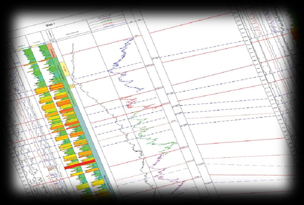
16 It will be necessary to experiment with the parameters; the following guidelines may help: Window is the length of the analysis window in depth units: start by using the default value (40m). (Note: when your data is in feet, use 120ft). The default Start and End depths include the entire log: change the depths if you wish to analyse only a part of the data. The Step size is the amount (in depth units) by which the window is moved at each step in the calculation. Start with the default value (1m). (Note: when your data is in feet, use 3ft). The Autocorrelation length should be set to approximately a quarter of the window length. (The default value for window length 40m is 9m.) (Note: when your data is in feet, use 27ft). The values of Minimum and Maximum Wavelength define the range of values shown on the horizontal scale of the finished power spectrum. Start with the defaults and adjust to different values if the results are not satisfactory. Vertical scaling is best kept to the default value of 1. In many cases, the power of the smaller wavelengths will be swamped by the large ones: in such cases check the Enhance small wavelengths box to correct for this effect. When all parameters are set, click OK in the Frequency Analysis dialog box. CycloLog runs the spectral analysis, and adds the result to the list of logs in the workspace. The name of the new log will be, for example, GR MESA. If you run a second analysis, its name will be GR MESA (2). To open the MESA results, double-click on its name in the workspace. The example below shows the result of a MESA analysis (Right pane) on the GR log displayed in the left pane. The vertical axis of the MESA display is depth, and the display scrolls with other logs from the same well. Version September 2016 ENRES International Page 15

17 To interpret the results, remember that the method uses a moving window of analysis. The power spectra resulting from analysis of each window are stacked up, such that the peaks in successive spectra line up to form ridges in the stack. The peaks are coloured to represent their relative height (i.e. amplitude), so that higher spectral ridges appear as brightly coloured streaks on the display. The horizontal scale of the display represents wavelength, decreasing logarithmically from left to right. (Longer wavelengths on the left; shorter wavelengths towards the right.) A vertical streak of bright colour indicates a wavelength that is persistently present through that interval of the log data. Although no horizontal scale is shown on the display, the wavelength of any peak at any depth can be found by using the cursor, as follows: To view the power spectrum at a single depth, move the cursor over the MESA log pane. The cursor changes into a horizontal line with five tick marks: Version September 2016 ENRES International Page 16

18 The second tick mark from the left is different from the others: it shows a cross. Position this cross mark over a spectral peak, and at a certain depth. The wavelength (Lambda) appears in the status bar at the bottom of the CycloLog screen. In the example above, the tick mark is set at Depth 3480m and the associated prominent wavelength, indicated as Lambda, has a frequency of 5.30m. To view the complete power spectrum at any depth, right-click over the GR - MESA data pane, to open a special context menu: Version September 2016 ENRES International Page 17

19 From this menu, select Toggle Average Spectrum. The Average Spectrum window opens. This window shows the Average Amplitude Spectrum, or power spectrum, at a single depth point (in the image above, at depth m); the spectrum changes as the cursor is moved up and down the GR - MESA data pane. The Amplitude is scaled vertically; the Wavelength (m) is shown on the horizontal axis, where it is plotted logarithmically, from higher values on the left, to lower values at the right. Version September 2016 ENRES International Page 18

20 2.4 Interpretation of Milankovitch cycles The result of a spectral analysis is a breakdown of the data into a set of simple (sine/cosine) waves. Deciding whether or not these have any geological and/or climatic significance is a matter of interpretation. E1 E2 O P1 P2 When the cursor is over the MESA display, it takes the form of a horizontal line with five tick marks, as in the above figure. The relative positions of the ticks represent (in terms of wavelength) the ratios among the principal predicted Milankovitch frequencies. From left to right along the cursor, these are: E1, long orbital eccentricity cycle: E2, short eccentricity cycle: O, axial obliquity cycle: P1, precession cycle: P2, precession cycle: 413ka 100ka 41ka 23ka 21ka Note that the logarithmic scale makes the 413ka and 100ka tick marks appear closer together than the 32ka and 19ka ticks! Note also that the relative positions of the predicted Milankovitch periods are also shown on the Average Amplitude Spectrum display: see the figure above in part 3.2. Version September 2016 ENRES International Page 19

21 By default, the 100ka tick is selected as the dominant frequency: it is distinguished from the others, by having a cross line through it. To change the dominant frequency, see further below. The Status Bar displays the frequency (Dom. freq.) and amplitude (Magn.) of the power spectrum at the point under the dominant tick mark. The Status Bar also provides two statistics designed to help in the identification of Milankovitch periods: Sedimentation rate: this is the net accumulation rate implied by the wavelength position corresponding to the position of the dominant frequency tick mark on the Milankovitch cursor (N = m/ka on the figure above). This assumes, of course, that deposition was continuous and at an unchanging rate, so must be used with care. MilaSum ( Mila on the Status Bar) is an arbitrary measure of the quality of the match between the predicted Milankovitch period ratios, and the ratios between the observed peaks, for the current position of the Milankovitch cursor. This statistic should also be used with care, but it may help with choosing between different interpretations. If a full suite of Milankovitch periods is perfectly represented in the stratigraphy, then the corresponding peaks in the MESA spectrum should all lie under one of the ticks on the Milankovitch cursor. Moving the cursor ticks with the mouse should indicate whether or not this is likely. Bear in mind that any interpretation in terms of Milankovitch cycle periods must be consistent with available evidence for the total duration of the succession. It is very rarely the case that all Milankovitch periods are represented. The user will therefore have to decide, (a) whether any of the spectral wavelengths are likely to represent Milankovitch periods, and, if so, (b) which wavelengths correspond to which of the predicted cycle periods. Version September 2016 ENRES International Page 20

22 2.5 Using the MESA menu Place the cursor over the GR - MESA data pane and right-click with the mouse to open a menu that contains a number of special functions. Analysis parameters shows a record of the parameters used to generate the MESA display. Toggle Average Spectrum was explained above; it can be toggled on/off. Geological Period (illustrated below). The ratios between the Milankovitch periodicities change through geological time; select the period most appropriate to the data being analysed. (See CycloLog Help for further information.) M-P Manager (on the Geological Period menu). Use this dialog box to change the periodicity selected as dominant (default 100ka). Version September 2016 ENRES International Page 21

23 Part 3 - Advanced log processing functions 3.1 Advanced processing functions in CycloLog CycloLog has a number of additional/advanced calculation and analysis functions. Introductory instructions for some of these functions are given in this section of the tutorial; others are explained in CycloLog Help. The functions covered here are: Synthetic seismogram generating simple seismic traces from logs Math Studio defining arithmetical combinations of logs Markov Chain Analysis analysing patterns of upward change 3.2 Generating synthetic seismograms Synthetic seismic traces can be generated in CycloLog, either automatically or manually. The automatic method is described here; the manual method is described in CycloLog Help. Go to the man menu bar and select Calculations Synthetic Seismogram. The following dialog window opens: Select the Well you wish to calculate a synthetic seismogram. Check the Domain. From the Sonic and Density drop-down lists, select the sonic and density logs that you wish to use in the calculation. Version September 2016 ENRES International Page 22

24 Select a Wavelet see below for information. Define the Wavelength (default = 10m). Click OK. The Synthetic Seismogram is generated, and added to the workspace. The above figure shows the synthetic seismogram displayed alongside the sonic and density curves from which it was generated. The display initially shows only a single trace, without toning. This is converted to a multiple trace display (as shown above) as follows: Make sure the synthetic seismogram pane is open and the active pane. Open the properties pane. Under Log appearance, set the Display mode to Pseudo section. Under Toning, set Use toning to True and set the Toning side, Tone color and Cutoff value. Note: Wavelet types available in the Synthetics Seismogram dialog are: Minimum Phase Wavelet Ricker Wavelet Type 1 (the standard Ricker wavelet) Ricker Wavelet types 2, 3 and 4 (Ricker wavelets with a more ringing character) Version September 2016 ENRES International Page 23

25 3.3 Using Math Studio The Math Studio consists of a range of calculations that can be performed on logs. Several basic calculations can be performed without using the Math Studio. Their use was described in part 1.3 of this tutorial, and they are: Add Logs (add one log to another) Subtract Logs (subtract one log from another) Multiply Logs (multiply one log by another) Divide Logs (divide one log by another) Integral (calculate the integral of a log curve) Derivative (calculate the derivative of a log curve) Logarithm (calculate the logarithm of all data values in a log) Exponent (calculate the inverse logarithm of all data values) For the above calculations, open the log that is to be the subject of the calculation (suggestion: use a copy of the log), right-click over the opened log pane and select Processing Log Calculations and then select the required operation. For more advanced calculations, use the Math Studio, as follows: From the main menu bar select Tools Math Studio. The Math Studio dialog box opens. It a number of tabs and other features, briefly explained in the following figure below. The Math Studio is used to set up formulas that will be applied to every depth point in a specified interval. The formulas can be set up by selecting the logs, the arithmetical operators, various available functions, and a selection of constants, from standard lists. Version September 2016 ENRES International Page 24

26 The Equations tab is where you will set up a formula, as in the example described below. The Logs tab has a list of all the logs of the selected well in the workspace, including logs that you have created such as cluster logs or synthetic seismograms. The Constants tab lists four basic constants (DZ, PI, ZMAX, and ZMIN). The Operators tab lists ten basic arithmetical operators (add, subtract etc.). The Functions tab lists twenty-six more advanced functions, including trigonometrical functions (sine, cosine, etc.), logarithms (natural and base 10), and exponentiation. Version September 2016 ENRES International Page 25

27 To demonstrate how to set up an equation, the following example calculates shale separation from the neutron and density curves, using the formula: 100*NPHI/0.6 + RHOB (This formula assumes that NPHI is expressed as a ratio; where NPHI is a percentage, the formula is NPHI/0.6 + RHOB - 2.7). Go to the Equations tab. Click in the Equation field, at the bottom of the dialog box. The following sequence of operations will construct the equation: Type 100. Go to the Operators tab and double-click on the multiply operator (*). Note that this operator is added to the Equation field. Go to the Logs tab and double-click on the NPHI log. Go to the Operators tab and double-click on the add operator (+). Go to the Logs tab and double-click on the RHOB log. Go to the Operators tab and double-click on the subtract operator (-). Type 2.7. The full formula now appears in the Equation field, as: 100*"NPHI"+"RHOB"-2.7 To save this formula: Click the Add button to open the Save Equation Dialog box. Type a name for the formula, and click OK. The formula has been saved for future use; it will now appear on the Equations tab every time you open the Math Studio. Version September 2016 ENRES International Page 26

28 To apply the formula: Check that the correct Well is selected at the top of the dialog box. Check that the equation is listed in Equation field (if not double-click on Shale separation in the equation list. Change the depth Interval if you do not want the formula applied to the entire data set. Click Calculate. CycloLog runs the calculation, and adds the results to the workspace as a new log with the name of the formula (in this case, the new log is called Shale Separation ). To save the formula for importing to another CycloLog project: Select the formula in the list on the Equations tab. Click Export and give the file a name (e.g., ShaleSeparation). The file will be saved as (for example) ShaleSeparation.equ. Version September 2016 ENRES International Page 27

29 3.4 Markov Chain Analysis in CycloLog Markov Chain Analysis in general looks for relationships between the current state of a process and its previous state. In stratigraphy, it is used for testing the relationships between adjacent lithologies in a stratigraphic succession: is the succession of lithologies purely random, or is there some order to the way in which lithologies succeed each other? No single log has a direct relationship with lithology; it is therefore necessary to start by defining the lithologies that the Markov Chain Analysis will work with. There are several ways to do this, but a good starting point is a Cluster Analysis, as described in Tutorial Clustering and Lithology, part 1. The following description of a Markov Chain Analysis in CycloLog is based on the result of the cluster analysis that was used as an example in the Tutorial Clustering and Lithology, part 1. The native clustering was based on the combination of the GR, sonic, neutron and density logs; it defined seven clusters. From the main menu bar select Analysis Markov Chain Analysis. On the General tab of the dialog box, select the Well and the Log on which the analysis will be based; in the example, this is the Cluster Log. Define the Top and Bottom depth interval for the analysis. Define the Step size; this is the size of the intervals into which the data will be divided into lithologies (1 meter in the example). Version September 2016 ENRES International Page 28

30 Now open the Lithology tab. Accept the default method: Automatic. See below concerning the other methods (Predefined model, and Manual). For the log on which the analysis is to be based, identify the Minimum and Maximum values of the log in the interval to be analysed. (In the example, the clusters are numbered from 0 to 7, so the minimum is 0 and the maximum is 7.) Define the Number of Intervals (i.e. lithologies ) into which the data are to be divided (7 in the example). Click OK. The analysis runs, and a Markov Chain Log is added to the list in the workspace. (This depicts the lithologies into which the chosen log has been subdivided for the analysis.) Version September 2016 ENRES International Page 29

31 The figure above shows the Cluster log (middle pane) which was used as the basis for subdivision into lithologies. In the Markov Chain Log (right hand pane), 7 lithologies (based on the clusters) are defined in 1m steps. The Markov Chain Analysis categorizes every upward transition, at every 1m step, and counts the resulting transitions. To view the results of the analysis: Open the new Markov Chain Log. Right-click over the opened Markov Chain Log pane and select Analysis Results. The following Markov Chain Analysis Results dialog box opens: Version September 2016 ENRES International Page 30

32 The analysis categorises and counts every upward transition from one lithology to the next. Note that, because all steps are the same size (1m in the example), many of the upward transitions will be self-transitions, at which the lithology stays the same. Based on these counts, the probability of every possible upward transition is calculated; if the data are not random, then some upward transitions will be more likely than others. The results box presents this information in three parts, two on the Matrix tab and one on the Significance tab. On the Matrix tab, the table of Observed transition probabilities shows the relative probabilities of every possible upward transition. (See the data on the Significance tab for the details of these results.) The table should be read from row to column. A few of these results are now discussed, to suggest how the results might be interpreted. In the example, lithology 1 is succeeded by itself with a high probability of Lithology 1 has the characteristics of a fine-grained sandstone; the high probability of an upward selftransition means that such sandstones are likely to occur in units greater than 1m in thickness. Lithologies 3 and 4 have lower probabilities of self-transition, so are more likely to occur in thinner beds. Version September 2016 ENRES International Page 31

33 Lithology 5 has a high probability (0.382) of upward transition to lithology 3, but zero probability of upward transition to lithology 1. Lithology 4 is quite likely (0.350) to be succeeded by lithology 2, but lithology 2 is much less likely (0.085) to be followed by lithology 4. Based on these transition probabilities, the Markov chains box on the Matrix tab shows the possible upward chains of lithological states, in decreasing order of their probability. Each such chain is a cycle in that it starts and finishes with the same lithology. In the example, there is a large number of possible chains, indicating that there is no one dominant cyclic or repetitive pattern. Looking at the first few in the example, and taking the Cluster Matrix of the Cluster Log analysis results into account (see below): The chain 3 > 1 > 3 occurs with the highest probability. Lithologies 1 and 3 both have low GR values (mean 33 and 52 API, respectively), so this chain expresses the moderate probability of switching between sandstones with slightly higher and slightly lower GR values. The next three chains are 3 > 2 > 3 with probability 0.171; and 5 > 3 > 2 > 5 (0.146). They represent variations on transitions among lithologies with mid- to high-range GR values. The following two chains contain rather more abrupt transitions: 5 > 2 > 5 (0.146); and 5 > 4 > 2 > 5 (0.146). Lithologies 2 and 5 are considerably more different in their GR values (mean 41 and 98 API, respectively). Clearly, the interpretation of the transition probabilities, whether pairwise or in chains, is highly dependent on an understanding of the lithofacies of the succession. Version September 2016 ENRES International Page 32

34 Part 4 - Basic petrophysical functions 4.1 Petrophysical functions in CycloLog CycloLog includes a number of basic petrophysical functions. Introductory instructions for these are given in this section of the tutorial. Functions covered here are: Porosity calculation Porosity calibration using core measurements Permeability calculation Water saturation calculation Water resistivity calculation Creating a petrophysical summary report 4.2 Porosity calculation In CycloLog, there are three different ways for calculting porosity estimations, starting from the following logs: Density log Sonic log Density and neutron logs You may wish to use more than one of these methods, depending on which logs are available, and to compare the results. All three options are selected from the Porosity menu: Go to the main menu bar and select: Petrophysics Porosity. Move the cursor to the Porosity item you wish to use. Select the required method. Version September 2016 ENRES International Page 33

35 4.3 Porosity calculation from a density log Calculation of porosity (φ density) from a density log uses the following formula: φ density = (ρ matrix ρ bulk) / (ρ matrix ρ fluid) where, ρ matrix ρ bulk ρ fluid = matrix (or grain) density = bulk density as measured by the logging tool = density of fluid So, as long as we can provide numbers for the matrix density (ρ matrix) and the fluid density (ρ fluid), this formula will give the porosity (in fraction between 0.0 and 1.0) from the density log (ρ bulk). If the lithology of the matrix is known, use the following standard density values (in g/cm 3 ): Sandstone (quartz) Limestone (calcite) Dolomite Gypsum Anhydrite Halite For the fluid density, use 1.0 g/cm 3 for freshwater, and 1.1 g/cm 3 for brine. Alternatively, the matrix density can be obtained directly from the log data, as explained below. To start the calculation: From the main menu bar, select: Petrophysics Porosity; Then select Use Density Log. The following dialog box opens: Version September 2016 ENRES International Page 34

36 Check that the correct Well is selected. Select the required density log from the drop-down list. Specify the Top and Bottom depth interval over which the porosity is to be calculated. Enter the Fluid density (in g/cm 3 ). See above. EITHER enter the Matrix density (if known). OR average the Matrix density from the data as follows: o Click on the Histogram icon next to the Matrix density box. o Hold the cursor over the value regarded as representing the appropriate density value, and click once with the left mouse button o A vertical red line marks the currently selected value. Version September 2016 ENRES International Page 35

37 o Click OK to enter this value into the Matrix density box in the Calculate porosity dialog box. Click OK to run the porosity calculation. CycloLog runs the calculation and creates a new log called Porosity <logname> (here: RHOB) that is saved to the workspace. Version September 2016 ENRES International Page 36

38 4.4 Porosity calculation from density and neutron logs The second method available in CycloLog calculates porosity (in %) from a combination of a density and a neutron log. The combined porosity (φ N - D) is calculated as the root-mean-square of the porosities from the density and neutron logs separately: φ N - D = ((φ N 2 + φ D2 ) / 2) 1/2 If the lithology of the matrix is known, use the following standard density values (in g/cm 3 ): Sandstone (quartz) Limestone (calcite) Dolomite Gypsum Anhydrite Halite For the fluid density, use 1.0 g/cm 3 for freshwater, and 1.1 g/cm 3 for brine. Alternatively, the matrix density can be obtained directly from the log data, as explained below. To start the calculation: From the main menu bar, select: Petrophysics Porosity. Then select Use Density and Neutron Log. The following dialog box opens: Version September 2016 ENRES International Page 37

39 Check that the correct Well is selected. Select the required Density log from the drop-down list. Select the required Neutron log from the drop-down list. Specify the Top and Bottom depth interval over which the porosity is to be calculated. Enter the Fluid density (in g/cm 3 ). EITHER enter the Matrix density (if known). OR average the Matrix density from the data as follows: o Click on the Histogram icon next to the Matrix density box. o o o Hold the cursor over the value regarded as representing the appropriate density value, and click once with the left mouse button. A vertical red line marks the currently selected value. Click OK to enter this value into the Matrix density box in the Calculate porosity dialogue box. Click OK to run the porosity calculation. CycloLog runs the calculation and creates a new log called Porosity <logname> (here: RHOB-NPHI). This log is added to the workspace tree. Version September 2016 ENRES International Page 38

40 4.5 Porosity calculation from a sonic log Porosity (φ sonic) may also be calculated from a sonic log if no density log is available, although the results may be less reliable. The calculation is based on the following formula: φ sonic = (Δt log Δt matrix) / (Δt fluid Δt matrix) where, Δt log Δt matrix Δt fluid = sonic log value (interval transit time) = interval transit time for the matrix = interval transit time for the fluid Given values for the interval transit time in the matrix and the pore fluid, this formula allows us to calculate sonic porosity from the values of the sonic log. If the lithology of the matrix is known, you may be able to use one of the following standard values (in μs/ft) for Δt matrix: Sandstones (quartz) Limestone (calcite) Dolomite 43.5 Gypsum Anhydrite 50 Halite 67.0 For the fluid interval transit time, use 189 μs/ft for freshwater-based mud, or 185 μs/ft for saltwaterbased mud. Alternatively, the matrix interval transit time can be obtained directly from the log data, as explained below. To start the calculation: From the main menu bar, select: Petrophysics Porosity. Then select Use Sonic Log. The following dialog box opens: Version September 2016 ENRES International Page 39

41 Check that the correct Well is selected. Select the required Sonic log from the drop-down list. Specify the Top and Bottom depth interval over which the porosity is to be calculated. Enter the Fluid interval transit time (in μs/ft); EITHER enter the Matrix interval transit time (if known). OR average the Matrix interval transit time from the data as follows: o o o o Click on the Histogram icon next to the Matrix interval transit time box. Hold the cursor over the peak regarded as representing the appropriate sonic value, and click once with the left mouse button. A vertical red line marks the currently selected value. Click OK to enter this value into the Matrix interval transit time box in the Calculate porosity dialog box; Click OK to run the porosity calculation. Version September 2016 ENRES International Page 40

42 CycloLog runs the calculation and creates a new log called Porosity <logname> (here: DT). This log is shown in the following illustration beside the original sonic (DT) log: Version September 2016 ENRES International Page 41

43 4.6 Porosity calibration If direct porosity measurements are available (from core samples, for example), these can be used to calibrate a log-derived porosity curve. Suppose that the following porosities have been measured on a core of the selected well, at the given depths: Depth Porosity 3372m m m m From the main menu bar, select Petrophysics Calibrate Porosity. In the dialog box that opens, select Well and Porosity log to be calibrated. Click Next. The Calibration with Core Plug Porosities dialog box opens: Enter the Depths and core porosity measurements (Por. Core) in the first and second columns. (Alternatively, if you have the values in a table like the one above, copy it to the clipboard, and click the Import button to paste the values into the dialog box). Version September 2016 ENRES International Page 42

44 Click Calculate, and CycloLog enters the porosity values from the selected log. (You can choose either to Interpolate between the values at the nearest depths, or Shift to nearest, to use the log value at the nearest available depth). Click Next. A graph of Core Porosity against Log Porosity opens, in which the black line represents a reference line when no calibration is needed, and the red line shows the relationship as calibrated with the core porosity measurements. The regression equation for the calibrated relationship is shown. Use the Print and Export buttons to print the graph, or to export it as an image file. If the graph is acceptable, click Finish to apply the calibration to all the points in the porosity log. The calibrated log is saved in the workspace as (for example) Porosity RHOB-NPHI-calibrated. Version September 2016 ENRES International Page 43

45 4.7 Permeability calculation Calculation of permeability in CycloLog requires (1) a porosity log, and (2) some core permeability measurements. The steps are the same as for Calibrate Porosity, above. That is: From the main menu bar, select Petrophysics Permeability. In the Calculate Permeability dialog, select the porosity log to be used (and the Top and Bottom depth interval, if relevant). Click Next. In the Permeability dialog box, enter the Depth and Permeability values for each available core permeability measurement. Click Calculate to find the corresponding log porosity values. Click Next. The graph and regression equation show the resulting relationship between core permeability and log porosity: if this is acceptable, click Finish. CycloLog applies the equation to all log values (in the specified depth interval) and creates a new log called, for example, Permeability from Porosity RHOB-NPHI. Version September 2016 ENRES International Page 44

46 4.8 Water saturation calculation Calculation of water saturation in CycloLog requires (1) a porosity log, and (2) the formation resistivity curve (or a deep resistivity log). To run a water saturation calculation: From the main menu bar, select Petrophysics Water Saturation Water Saturation. The Calculate Water Saturation dialog box opens: The box shows the formula used to calculate water saturation. Under Input logs, select the Well, its Domain, the Formation resistivity log and the Porosity log to be used. Under Interval, enter the Top and Bottom depths of the interval of calculation. Add a non-zero value for the Water resistivity. Either accept the default values for the Tortuosity factor, Cementation exponent, and Saturation exponent, or enter your preferred values. Click OK. CycloLog calculates the new log, and saves it in the workspace as Water Saturation Curve. Version September 2016 ENRES International Page 45

47 4.9 Water resistivity calculation Calculation of water resistivity in CycloLog requires (1) a porosity log, and (2) the formation resistivity curve (or a deep resistivity log). To run a water saturation calculation: From the main menu bar, select Petrophysics Water Saturation Water Resistivity Curve. The Water Resistivity Curve dialog box opens: Under Input logs, select the Well, its Domain, the Formation resistivity log and the Porosity log to be used. Under Interval, enter the Top and Bottom depths of the interval of calculation. Either accept the default values for the Tortuosity factor, and Cementation exponent, or enter your preferred values. Click OK; CycloLog calculates the new log and saves it in the workspace as Water Resistivity Curve. Version September 2016 ENRES International Page 46

48 4.10 Generate petrophysical report The Petrophysical Report function in CycloLog can be used to generate a simple N/G report, or other similar types of report. The report can be generated for a total interval, or the total interval can be subdivided, the subdivisions being based on a pre-defined set of either Breaks (see Tutorial Base Module, part 5), or Reservoirs (see Tutorial Base Module, part 6). To generate a Petrophysical Report: Go to the main menu bar and select: Analysis Report. The Generate Report dialog box opens: In the example above, the analysis will look for all depths in the Porosity RHOB-NPHI log for which the value is greater than or equal to 15. Specify the Top and Bottom depth interval for the analysis. Version September 2016 ENRES International Page 47

49 Click a row under the column Log, to reveal a drop-down list. Select the log you wish to analyse. Click under Operator and select the operator to be used (>=, meaning greater-than-or-equalto, in the example illustrated). Under Value, enter the target value (15 in the example). Click Report. The following window opens: This shows the results of the analysis: for the specified depth interval, the criterion Porosity 15 is satisfied in 76.2m out of the total of 340m, with an average N/G of in the net interval. Click Save to save these results to a file, then Click Close to close the report window. The Generate Report dialog also offers a Generate Log button. This generates a simple log in which the value 1 indicates that the condition (e.g., Porosity 15) is satisfied at that depth, and 0 indicates that it is not satisfied. The log is added to the workspace, and is called Report Log. This log can be used, for example, to colour a GR log to show the intervals in which the porosity is greater than 15%. (Open the GR log, open the properties pane, under Log Fill select Fill with. Select Log and then select the Report Log in the dropdown menu). Version September 2016 ENRES International Page 48

50 Part 5 - Total Organic Carbon (TOC) 5.1 TOC calculation method in CycloLog The Total Organic Carbon (TOC) curve is calculated in CycloLog based on the method as described in Passey et al. (2009). This method, the Δ log R technique, applies the overlaying of a porosity log on a resistivity curve. In their paper, a combination of the transit-time curve (sonic, in µsec/ft) and resistivity curve (in ohm) is used. The following log combinations can be used in CycloLog: resistivity sonic resistivity neutron resistivity density Note that each log must be specified in the following units: Log Resistivity Sonic Units ohmm µsec/ft Neutron V/V (0 100) Density g/cm3 Version September 2016 ENRES International Page 49

51 5.2 TOC workflow in CycloLog In this workflow, the resistivity and the sonic curves are used to calculate the TOC content in a well. The curves will be overlain and baselined in a fine-grained, non-source, rock interval. With the baseline established, organic-rich intervals can be recognised by separation of the two curves, which is the Δ log R. The Δ log R is linearly related to TOC and is a function of maturity. Therefore, the maturity (in level of organic metamorphism units, LOM) is needed. If the LOM value is not known, it can be derived from measured vitrinite reflectance values (Hood et al., 1975). The well should be subdivided into several intervals, if multiple (and different) levels of maturity are present. To determine TOC, start with displaying the resistivity and the sonic curve in an overlay pane: In the main menu bar, select View Log Overlay. Select from the Log Overlay View dialogue box the logs to be displayed: the resistivity and sonic logs. Right-click over the overlay pane and select Analysis Total Organic Carbon. The Total Organic Carbon dialog window appears, showing four input fields. In the Identify logs, select the logs as used in the overlay pane: in the topmost input field select the Resistivity curve. In the lower left hand input field select one of the three log families (Sonic, Density, or Neutron), in this example the Sonic log, then select the corresponding curve in the right hand input field. Version September 2016 ENRES International Page 50

52 Click on the Activate button. In the Analysis Interval field, click on each of the edit buttons next to the Top and Bottom input fields. The Select Depth dialog window appears. In this dialog window, three options for selecting the depth interval are available: Version September 2016 ENRES International Page 51

53 o o o In the Manual option, enter a Depth or click on the Top or Bottom button. The Break option allows you to select a depth interval delineated by breaks. When a Break set is selected, all breaks within the set are listed in the menu below. Choose the desired Break. The Reservoir option allows you to select the top or bottom of a reservoir interval. When a Reservoir set is selected, all reservoirs within the set are listed in the menu below. Choose the desired Reservoir. In the Top/Bottom selection field, choose the Reservoir top or bottom for the desired depth interval. After you have finished with the depth interval selection, click on the OK button. Prior to the Scaling, go to the Level Of Maturity field and a value in the Select LOM field. In the Scaling field, you can calculate the TOC curve. This can be done in two ways: The first way uses a calibration interval from the two overlay curves. In an interval where the two curves overlay, it is assumed that this is a non-organic clay rich interval, and is used to calibrate the TOC calculation: o Use the green arrow buttons to shift the two curves over each other. In the Overlay log pane you can see how the curves are being shifted. o Click the log R button, the separation between the two curves is calculated and added to the workspace. o Click the TOC button, the level of maturity is used to convert the separation between the two curves into a TOC curve which is added to the workspace. Version September 2016 ENRES International Page 52

54 The second way uses TOC measurements for calibrating the TOC curve: o o o o o o Click on the Calibrate button. The Calibrate window appears where you can import the measured TOC data points. Click the Calculate button in the Calibrate window. The scaling value for the resistivity curve is calculated. Close the window. Back in the Scaling box in the Total Organic Carbon window, determine an average resistivity scaling value and fill this value in the Resistivity max field. Click on the Set button. The scaling of the curves in the overlay pane is adjusted according to your settings. Click the log R button, the separation between the two curves is calculated and added to the workspace. Click the TOC button, the selected level of maturity is used to convert the separation between the two curves into a TOC curve. References Hood, A., Gutjahr, C. C. M., and Heacock, R. l., Organic metamorphism and the generation of petroleum: AAPG Bulletin. V. 59, No. 6, P Passey, O. R., Creaney, S., Kulla, J. B., Moretti, F. J., and Stroud, J. D., A practical model for organic richness from porosity and resistivity logs: AAPG Bulletin. V. 74, No. 12, P Version September 2016 ENRES International Page 53