Gas-liquid mass transfer in an external airlift loop reactor for syngas fermentation

Transcription

1 Retrospective Theses and Dissertations 2007 Gas-liquid mass transfer in an external airlift loop reactor for syngas fermentation Samuel T. Jones Iowa State University Follow this and additional works at: Part of the Chemical Engineering Commons, and the Mechanical Engineering Commons Recommended Citation Jones, Samuel T., "Gas-liquid mass transfer in an external airlift loop reactor for syngas fermentation" (2007). Retrospective Theses and Dissertations This Dissertation is brought to you for free and open access by Iowa State University Digital Repository. It has been accepted for inclusion in Retrospective Theses and Dissertations by an authorized administrator of Iowa State University Digital Repository. For more information, please contact

2 Gas-liquid mass transfer in an external airlift loop reactor for syngas fermentation by Samuel T. Jones A dissertation submitted to the graduate faculty in partial fulfillment of the requirements for the degree of DOCTOR OF PHILOSOPHY Co-majors: Mechanical Engineering; Biorenewable Resources and Technology Program of Study Committee: Theodore J. Heindel, Major Professor Robert C. Brown Gerald M. Colver Alan A. Dispirito Jacqueline V. Shanks Iowa State University Ames, Iowa 2007 Copyright Samuel T. Jones, All rights reserved.

3 UMI Number: UMI Microform Copyright 2007 by ProQuest Information and Learning Company. All rights reserved. This microform edition is protected against unauthorized copying under Title 17, United States Code. ProQuest Information and Learning Company 300 North Zeeb Road P.O. Box 1346 Ann Arbor, MI

4 ii TABLE OF CONTENTS List of Figures... vi List of Tables...xiii Nomenclature... xiv Abstract... xix Acknowledgements... xxi Chapter 1: Introduction Motivation Objectives... 2 Chapter 2: Literature Review Bioreactors Applications Types Selection Airlift Reactor Fundamentals Superficial Gas Velocity Gas Holdup Slip Velocity Mixing Time Superficial Liquid Velocity Flow Regimes Area Ratio Overall Gas-Liquid Mass Transfer Coefficient Airlift Reactor Performance Height Gas Separator Area Ratio Gas Sparger Internals Liquid Phase Properties and Hydrodynamics Liquid Phase Properties and Mass Transfer Solid Particles Performance Summary... 54

5 iii 2.4 Dissolved Oxygen Measurement Techniques Chemical Method Volumetric Method Tubing Method Optode Method Electrochemical Electrode Method Dissolved Carbon Monoxide Measurement Determining k L a Gas Balance Method Dynamic Method Chemical Sorption Methods Summary Chapter 3: Equipment and Experimental Methods External Airlift Loop Reactor Setup Data Acquisition System Working Fluid/Water Quality Aerator Plates Superficial Gas Velocity Reactor Modes of Operation Visual Flow Observations Visual Flow Observation Experimental Setup Visual Flow Observation Method Gas Holdup Measurement Riser Gas Holdup (ε r ) Downcomer Gas Holdup (ε d ) Superficial Liquid Velocity Measurement Test Equipment Test Reagents Linear Velocity Measurement Superficial Liquid Velocity Calculations Dynamic Gassing Out Method Basic Dynamic Gassing Out Method Expanded Dynamic Gassing Out Method Dynamic Gassing Out Method Step Time Dissolved Oxygen Measurement Experimental Equipment Electrode Preparation Gas Flow Rates

6 iv Dissolved Oxygen Concentration Measurement Dissolved Carbon Monoxide Measurement Safety Equipment and Reagents Liquid Samples Collection Reagent Preparation Bioassay Measuring Absorbance Spectrums Bioassay Spectral Fitting Volumetric Mass Transfer Coefficient (k L a) Determination Measurement Uncertainty Summary Chapter 4: Results Visual Observations Upper Connector Region Visual Observations Visual Observations Bottom of the Downcomer Gas Holdup Tap Water Gas Holdup Deionized Water Gas Holdup KCl Solution and Nitrosomonas Solution Gas Holdup Gas Holdup Correlations Liquid Velocity Tap Water Liquid Velocity Deionized Water, KCl Solution, and Nitrosomonas Solution Liquid Velocity Tap Water Liquid Velocity Correlations Gas-Liquid Mass Transfer Oxygen Gas-Liquid Mass Transfer Carbon Monoxide Gas-Liquid Mass Transfer Oxygen and Carbon Monoxide Gas-Liquid Mass Transfer Comparison Gas-Liquid Mass Transfer Correlations Chapter 5: Conclusions and Recommendations Conclusions Recommendations References Appendix A: Pressure Transducer Determination of Fractional Gas Holdup. 211

7 v Appendix B: Digital Images Collected for Visual Observations Appendix C: Hydrodynamic Data Appendix D: Gas-Liquid Mass Transfer Data

8 vi LIST OF FIGURES Figure 2.1: Basic sparged reactor types commonly used for industrial and biochemical applications... 7 Figure 2.2: Figure 2.3: Figure 2.4: Figure 2.5: Figure 2.6: Internal and external loop reactor configurations common encountered in the literature External airlift loop reactor schematic showing the four basic reactor sections Possible operating conditions for BCRs and ALRs, adopted from Merchuk [22] Typical hydrodynamic flow regime encountered in ALRs, adopted from Chisti and Moo-Young [18] Mass transfer resistances encountered in gas-liquid dispersions containing active cells, adapted from Chisti [2] Figure 2.7: Gas separators commonly encounter in external airlift loop reactors Figure 2.8: Figure 2.9: Figure 2.10: Figure 2.11: Figure 2.12: Figure 2.13: Dynamic gas spargers commonly used in pneumatic gas-liquid reactors, adopted from van Dam-Mieras et al. [51] Static spargers commonly encounter in pneumatic gas-liquid reactors, adapted from van Dam-Mieras et al. [51] Fluid flow patterns observed in external airlift loop reactors for two reactor base styles, adopted from Chisti [2] Diagram showing the relationship between design and operating variables and their effect on airlift loop reactor performance, compiled from the literature [2, 6, 19, 82, 83] Schematics showing the typically construction of polarographic and galvanic electrodes, adopted from Linek [94] Typical polarographic electrode polarogram, adopted from Lee and Tsao [95]... 64

9 vii Figure 2.14: The typical oxygen transport path encountered at an electrode tip Figure 2.15: Figure 2.16: Figure 2.17: One and three layer electrode models used to estimate electrode time constants, adopted from Linek [94] Typical dissolved oxygen concentration variation with time for the biological dynamic method, adopted from Blanch and Clark [127] Typical dissolved oxygen concentration variation with time for the nonbiological dynamic method, adapted from Blanch and Clark [127] Figure 3.1: External airlift loop reactor used in this study Figure 3.2: Figure 3.3: Schematic representation of the external airlift loop reactor showing the key components Close up view of the external loop airlift reactor riser showing the layout of the sample ports on the riser Figure 3.4: Experimental instrumentation panel Figure 3.5: Aerator plates used in the external airlift loop reactor Figure 3.6: Figure 3.7: Schematic representation of the external airlift loop reactor illustrating the three possible operational modes; open vent mode, closed vent mode, and bubble column mode Salt solution injector used to measure the linear velocity in the downcomer Figure 3.8: Microelectrode, Inc. miniature conductivity electrodes Figure 3.9: Typical conductivity electrode responses used to find the linear velocity Figure 3.10: Generic dissolved oxygen concentration as a function of time for the basic and the extended gassing out methods Figure 3.11: Diamond General Development Corp. dissolved oxygen electrode

10 viii Figure 3.12: Electrode chlorider, o-ring applicator, membranes, and o-rings used to maintain the oxygen electrode Figure 3.13: Installing a new membrane with the o-ring applicator Figure 3.14: Cole Parmer oxygen meter Figure 3.15: Schematic showing how the chloride layer is applied to the oxygen electrode Figure 3.16: Apparatus used to determine the electrode time constant Figure 3.17: Ocean Optics USB2000 spectrophotometer Figure 3.18: Syringes and cuvette used in the bioassay Figure 3.19: Sample syringes inserted in the external airlift loop reactor for liquid sample collection Figure 3.20: Reference absorbance spectrums Figure 3.21: Figure 3.22: Figure 3.23: Figure 3.24: Figure 3.25: Absorbance spectra progression from carbon monoxide free state to a carbon monoxide saturated state An illustration of how Equations (3.10) and (3.11) fit the experimental data when τ e << 1/k L a An illustration of how Equations (3.10) and (3.11) fit the experimental data when the difference between τ e and1/k L a is about one order of magnitude An illustration of how Equations (3.10) and (3.11) fit the experimental data when the difference between τ e and1/k L a is less than one order of magnitude Typical dissolved carbon monoxide data and the corresponding k L a value found using a nonlinear fitting routine to Equation (3.10)

11 ix Figure 3.26: Figure 4.1: Figure 4.2: Figure 4.3: Figure 4.4: Figure 4.5: Figure 4.6: Figure 4.7: Figure 4.8: Figure 4.9: Figure 4.10: Figure 4.11: Figure 4.12: Typical dissolved oxygen data and the corresponding k L a value found using a nonlinear fitting routine to Equation (3.11) External airlift loop reactor flow behavior at the upper connector for open vent mode and U G = 0.5 cm/s External airlift loop reactor flow behavior at the upper connector for open vent mode and U G = 3.5 cm/s External airlift loop reactor flow behavior at the upper connector for open vent mode and U G = 10.0 cm/s External airlift loop reactor flow behavior at the upper connector for open vent mode and U G = 20.0 cm/s External airlift loop reactor flow behavior at the upper connector for closed vent mode and U G = 0.5 cm/s External airlift loop reactor flow behavior at the upper connector for closed vent mode and U G = 7.0 cm/s External airlift loop reactor flow behavior at the upper connector for closed vent mode and U G = 20.0 cm/s External loop reactor flow behavior and gas holdup in the bottom of the downcomer for open vent mode External loop reactor flow behavior and gas holdup in the bottom of the downcomer for closed vent mode Gas holdup using different aeration plates when the external airlift loop reactor is operated in bubble column mode Effect of external airlift loop reactor operation mode on gas holdup for A = 0.62% Aerator plate open area ratio effect on gas holdup for open vent mode external airlift loop reactor operation

12 x Figure 4.13: Figure 4.14: Figure 4.15: Figure 4.16: Figure 4.17: Figure 4.18: Figure 4.19: Figure 4.20: Figure 4.21: Figure 4.22: Figure 4.23: Gas holdup as a function of superficial liquid velocity and external airlift loop reactor operation using deionized water when A = 0.62% Gas holdup as a function of superficial liquid velocity and aerator plate open area using deionized water for the OV mode of external airlift loop reactor operation Gas holdup as a function of superficial liquid velocity and fluid type for the OV mode external airlift loop reactor where A = 0.62% Variation in riser gas holdup correlations used to predict gas holdup in an external airlift loop reactor. See Table 4.1 for correlation legend Parity plot of the tap water riser gas holdup correlation expressed by Equation (4.1) using the coefficients and exponents shown in Table Aerator plate open area ratio and mode of operation effects on riser superficial liquid velocity Relationship between driving force (ε r ε d ) and superficial liquid velocity as a function of aerator plate open area ratio for the open vent mode external airlift loop reactor operation Relationship between driving force (ε r ε d ) and superficial liquid velocity as a function of aerator plate open area ratio for the closed vent mode external airlift loop reactor operation Aerator plate open area ratio and mode of operation effects on riser superficial liquid velocity for deionized water Liquid medium and mode of operation effects on riser superficial liquid velocities for A = 0.62% Riser superficial liquid velocity in external airlift loop reactors as a function of superficial gas velocity for reactors with similar geometric configurations and downcomer to riser cross sectional area ratios that range from 0.04 to Figure 4.24: Parity plot of the U Lr correlation expressed by Equations (4.2) and (4.3)

13 xi Figure 4.25: Figure 4.26: Figure 4.27: Figure 4.28: Figure 4.29: Figure 4.30: Figure 4.31: Figure 4.32: Figure 4.33: Figure 4.34: Oxygen volumetric mass transfer coefficient shown as a function of U G and external airlift loop reactor mode of operation for A = 0.62% and deionized water Oxygen volumetric mass transfer coefficient shown as a function of U G and aerator plate open area ratio for external airlift loop reactor open vent mode of operation and deionized water Oxygen volumetric mass transfer coefficient shown as a function of U G and fluid type for A = 0.62% and external airlift loop reactor open vent mode of operation External airlift loop reactor volumetric oxygen mass transfer rate as a function of superficial gas velocity and mode of operation for A = 0.62% Carbon monoxide volumetric mass transfer coefficient shown as a function of U G and external airlift loop reactor mode of operation for A = 0.62% and deionized water Carbon monoxide volumetric mass transfer coefficient shown as a function of U G and aerator plate open area ratio for external airlift loop reactor open vent mode of operation and deionized water Carbon monoxide volumetric mass transfer coefficient shown as a function of U G and fluid type for A = 0.62% and external airlift loop reactor open vent mode of operation The theoretical relationship between oxygen and carbon monoxide mass transfer coefficients based upon the mass transfer models presented in Section A comparison of carbon monoxide and oxygen gas-liquid mass transfer data for the open vent mode of external loop airlift reactor using deionized water showing how Equation (4.4) fits the data when n = A comparison of carbon monoxide and oxygen gas-liquid mass transfer data for A = 0.62% using deionized water showing how Equation (4.4) fits the data when n =

14 xii Figure 4.35: Figure 4.36: Figure 4.37: Figure 4.38: A comparison of carbon monoxide and oxygen gas-liquid mass transfer data for A = 0.62% using the KCl and nitrosomonas solutions showing how Equation (4.4) fits the data when n = A comparison of carbon monoxide and oxygen gas-liquid mass transfer data for A = 0.62% using the deionized water with a surfactant showing how Equation (4.4) fits the data when n = A comparison of carbon monoxide and oxygen gas-liquid mass transfer data showing how Equation (4.4) fits the data when n = Mass transfer coefficients plotted as a function of riser gas holdup for all test conditions expect for those containing the surfactant Figure 4.39: Mass transfer coefficients predicted by Equation (4.5)

15 xiii LIST OF TABLES Table 3.1: The aerator plate open area ratios and corresponding 1 mm orifice count used in the external airlift loop reactor Table 3.2: The superficial gas velocities used this work Table 3.3 Number of samples taken to determine downcomer gas holdup Table 4.1: Table 4.2: Table 4.3: Summary of the correlations selected from the literature relating gas holdup to superficial gas velocity and external airlift loop reactor geometries and used in Figure Tap water riser gas holdup correlation coefficients and exponents for Equation (4.1) shown in Figure Riser superficial liquid velocity correlation coefficients and exponents for Equations (4.2) and (4.3) shown in Figure

16 xiv NOMENCLATURE Abbreviations ALR Airlift loop reactor BC BCR Bubble column Bubble column reactor CSTR Continuous stirred tank reactor CV Closed vent EALR External airlift loop reactor OV KCl Open vent Potassium chloride Roman Symbols a L Gas-liquid interfacial area per unit liquid volume (cm -1 ) A Aerator plate open area ratio (%) Abs Absorption value (-) A d Downcomer cross-sectional area (cm 2 ) AR Reactor downcomer to riser cross-sectional area ratio (-) A r Riser cross-sectional area (cm 2 ) Av Camera f-stop (-) C Molar concentration (μm) C * Gas-Liquid interface equilibrium molar concentration (μm)

17 xv C E Uncorrected molar concentration from the oxygen electrode (μm) C G Gas phase molar concentration (μm) C Gi Gas phase interface molar concentration (μm) C L Liquid phase molar concentration (μm) C Li Liquid phase interface molar concentration (μm) C Lss Steady state liquid phase molar concentration (μm) C o Steady state concentration at t = 0 (μm) C p Myoglobin concentration (μm) ΔC Molar concentration gradient (μm) d e Distance between the conductivity electrodes (cm) d m Oxygen electrode membrane thickness (mm) D Diffusivity (cm 2 s -1 ) D L Liquid film diffusivity (cm 2 s -1 ) D m Oxygen electrode membrane diffusivity (cm 2 s -1 ) DR Dilution ratio (-) E D Eddy diffusivity F Volumetric flow rate (cm 3 s -1 ) G G Volumetric gas flow rate (cm 3 s -1 ) GTR Molar gas mass transfer rate (μm s -1 ) Δh d Distance between the manometer ports on the reactor (cm) Δh m Manometer liquid height change (cm)

18 xvi H Height above the aerator plate (cm) H v Unaerated liquid height above the aerator plate (cm) H Henry s Constant (-) J A Molar flux (kmoles cm -2 s -1 ) k Mass transfer coefficient (cm s -1 ) k G Gas film mass transfer coefficient (cm s -1 ) k L Liquid film mass transfer coefficient (cm s -1 ) k L a Overall volumetric mass transfer coefficient based on liquid film (s -1 ) K Conductivity electrode constant (-) K L Overall mass transfer coefficient based on liquid film (cm s -1 ) M Molarity (moles L -1 ) n Exponent (-) ΔP Pressure gradient (cm H 2 O) ΔP o Liquid hydrostatic head when U G = 0 (cm H 2 O) qx Microbial gas conversion rate (kmoles cm -3 s -1 ) s Surface renewal rate (s) SS Percent of saturated carbon monoxide spectrum (%) t time (s) t c Circulation time (s) t e Exposure time (s) t p Time between the conductivity electrode signal peaks (s)

19 xvii Tv Camera shutter speed (s) U G Superficial gas velocity (cm s -1 ) U L Superficial liquid velocity (cm s -1 ) U Ld Downcomer superficial liquid velocity (cm s -1 ) U Lr Riser superficial liquid velocity (cm s -1 ) V L Interstitial liquid velocity (linear velocity) (cm s -1 ) V Ld Downcomer interstitial liquid velocity (linear velocity) (cm s -1 ) V Lr Riser interstitial liquid velocity (linear velocity) (cm s -1 ) Vol G Total reactor dispersed gas volume (cm 3 ) Vol L Total reactor unaerated liquid volume (cm 3 ) Vol S Sample volume in cuvette (μl) Vol T Total liquid volume in cuvettes (ml) x c Circulation path length (cm) Δx Film thickness (cm) Greek Symbols ε Overall gas holdup (-) ε d Downcomer gas holdup (-) ε m Protein extinction coefficient (μm -1 cm -1 ) ε r Riser gas holdup (-) π pi (-)

20 xviii ρ G Gas phase density (kg cm -3 ) ρ L Liquid phase density (kg cm -3 ) τ d Oxygen electrode lag time (s) τ d Reactor gas phase residence time (s) τ e Oxygen electrode time constant (s)

21 xix ABSTRACT Converting biomass to useful products through synthesis gas (syngas) fermentation has the potential to replace petroleum based products with biobased ones; however, these process are limited in their application. One of the most significant limiting steps in syngas fermentations is the gas-liquid mass transfer in the bioreactor due to the low solubilities of the major syngas components, CO and H 2. Hence, to explore possible solutions for over coming the gas-liquid mass transfer barrier, a non-traditional external airlift loop reactor is considered. This study evaluates the hydrodynamics and gas-liquid mass transfer rates in an external airlift loop reactor with an area ratio of 1:16 operating under different conditions. Two downcomer configurations are investigated consisting of the downcomer vent open or closed to the atmosphere. Experiments for these two configurations are carried out over a range of superficial gas velocities (U G ) from U G = 0.5 to 20 cm/s using three aeration plates with open area ratios of 0.66, 0.99 and 2.22%. These results are compared to a bubble column operating under similar conditions. Water quality variations are also investigated over the same range of U G with the downcomer open to the atmosphere. Experimental results show that the gas holdup in the riser does not vary significantly with a change in the downcomer configuration or bubble column operation, while a considerable variation is observed in the downcomer gas holdup. Gas holdup in both the riser and downcomer are found to increase with increasing superficial gas velocity. Test results also show that the maximum gas holdup for the three aeration plates is similar, but that the gas holdup trends are different. The superficial liquid velocity is found to vary considerably for the two

22 xx downcomer configurations. However, for both cases, the superficial liquid velocity is a function of the superficial gas velocity and/or the flow condition in the downcomer. These observed variations are independent of the aerator plate open area ratio. Gas-liquid mass transfer results indicate that mass transfer rates do vary for oxygen and carbon monoxide gas species. Gas-liquid mass transfer rates are observed to increase linearly with U G in the presence of a surfactant and to increase similarly to riser gas holdup with U G for deionized water and ionic solutions. The gas-liquid mass transfer rates are relatively unaffected by the reactor configuration. The results also show that the addition of a surfactant or ionic compounds has a significant effect on mass transfer, where the surfactant restricts gas-liquid mass transfer and the ionic compounds enhance gas-liquid mass transfer.

23 xxi ACKNOWLEDGEMENTS This material is based upon work supported by the Natural Resources Conservation Service, U.S. Department of Agriculture, under Agreement No. NRCS Any opinions, findings, conclusions, or recommendations expressed herein are those of the authors and do not necessarily reflect the views of the USDA. The author acknowledges all the members of his program of study committee, especially Dr. Theodore Heindel for his valuable insight, support, patience, and friendship that have been generously given over the past several years. The author also wishes to acknowledge Dr. Mark Hargrove and the undergraduate students who have assisted with this project. Finally, thanks must be given to my wife and family for their love, encouragement, patience, and sacrifice.

24 1 CHAPTER 1: INTRODUCTION 1.1 Motivation Materials and energy derived from biomass offer an alternative to conventional petroleum sources that would support national economic growth, national security, and reduce national dependence on imported petroleum sources. Currently, the popular method for converting biomass to energy, specifically ethanol, is the sugar to ethanol process. Another method that may be used to convert biomass to energy and other useful compounds is the thermochemical process. The thermochemical process relies on gasifying biomass to create synthesis gas (syngas) which is primarily a mixture of gaseous hydrogen, carbon monoxide, and carbon dioxide. Syngas may be converted biologically or chemically to compounds that can be used to displace traditional petroleum based compounds. The biological approach to converting syngas to useful products relies on using microorganisms to metabolize the carbon monoxide and hydrogen to compounds that can be used as a feedstock for biopolymers. However, because of the very low aqueous solubilities of carbon monoxide and hydrogen, syngas fermentations are limited by the low gas-liquid mass transfer rates. Hence, if the gas-liquid mass transfer road block can be removed, syngas fermentations could become the preferred method for converting biomass to petroleum substitutes. The use of mechanically agitated reactors in biological applications have been extensively studied over the past several decades and are widely used in some industrial

25 2 settings. However, these bioreactors have been found to have mixing characteristics that may adversely affect cell growth [1-6]. Thus, there is great interest in using pneumatically agitated bioreactors for processes such as syngas fermentation. Like mechanically agitated bioreactors, pneumatically agitated bioreactors have been studied over the last several decades; however, these bioreactors have not received as much attention and are not used as extensively in commercial applications. The design of pneumatically agitated bioreactors, unlike their mechanically agitated counter parts, varies widely and, as a result, the hydrodynamic and mass transfer characteristics of these bioreactors are often system dependent, hindering their wide spread implementation. To facilitate their use, a better understanding of reactor hydrodynamics and gas-liquid mass transfer characteristics is needed. 1.2 Objectives This research will focus on investigating transport phenomena in an external airlift loop reactor related to oxygen and carbon monoxide uptake in liquid media. This will be accomplished by completion of the following objectives: Objective 1: Review the literature related to transport phenomena in airlift loop reactors to understand hydrodynamic and gas-liquid mass transfer fundamentals for this reactor type. Objective 2: Measure gas holdup and liquid velocity to explore the hydrodynamics in an external airlift loop reactor with a downcomer to riser area ratio of 1:16.

26 3 2a: Study how reactor hydrodynamics vary with volumetric flow rate by altering the operational mode of the external airlift loop reactor. 2b: Assess the affect of aerator plate open area ratio on fluid dynamics for the operating conditions studied in 2a above. 2c: Evaluate the influence of water quality on hydrodynamics for the conditions considered in 2a and 2b above. Objective 3: Simplify the bioassay method used to quantify dissolved carbon monoxide concentration. Objective 4: Measure and compare the gas-liquid volumetric mass transfer rates for an external airlift loop reactor using the dynamic gassing out method for oxygen (with a dissolved oxygen electrode) and carbon monoxide (with a bioassay). 4a: Quantify how the gas-liquid volumetric mass transfer rate varies with the operational mode of the external airlift loop reactor. 4b: Determine the affect of aerator plate open area ratio on gas-liquid mass transfer for the operating conditions in 4a above. 4c: Consider the impact of water quality on gas-liquid mass transfer rates by studying and quantify how water quality impacts mass transfer for the conditions studied in 4a and 4b above. Objective 5: Compare the gas-liquid mass transfer data for oxygen and carbon monoxide and verify methods used to estimate one from the other.

27 4 The remainder of this dissertation expands on the above objectives. Chapter 2 reviews airlift loop reactor hydrodynamics, the factors known to affect hydrodynamics, the methods used to measure gas-liquid mass transfer, and the factors known to impact gas-liquid mass transfer with an emphasis being placed on the external airlift loop reactors. Chapter 3 addresses the methods and equipment used to quantify reactor hydrodynamics and gas-liquid mass transfer rates. Chapter 4 presents and discusses selected gas holdup, superficial liquid velocity, and gas-liquid mass transfer results. Chapter 5 briefly summarizes the trends and conclusions presented in Chapter 4 and well as presents some suggestions for future work.

28 5 CHAPTER 2: LITERATURE REVIEW This chapter is composed of four major sections. The first section reviews bioreactor applications and types with a focus on external airlift loop reactors. The second section presents the fundamental terminology related to airlift loop reactors. The third section discusses airlift loop reactor performance. The fourth section reviews methods used to measure gas-liquid mass transfer rates. 2.1 Bioreactors A reactor in the most general form is simply defined as a vat or tank for chemical reaction. Reactors used in modern industrial settings vary from simple tanks, where two or more chemicals are allowed to react, to more complex systems with agitators, baffles, static mixers, heat coils, cooling jackets, etc. to facilitate the production of a desired product. The term bioreactor has been coined to describe a special class of reactors used in biological processes. Like reactors, bioreactors vary in shape, size, and complexity depending on the requirements of the application. For example, bioreactors may be as simple as an ensilaging bag used to ferment and store biomass, to as complex as a chemostat used to culture artificial tissues and organs. Regardless of the design and application, most bioreactors fall into one of three general categories: (i) a simple tank reactor, (ii) an agitated tank reactor, and (iii) a flow reactor. The focus of this work deals with the agitated reactor.

29 Applications Bioreactors are used in many industrial applications around the world and thus it is not feasible here to discuss all the possible applications. Suffice it to say that these applications vary from simple sugar fermentations to very complex processes that cultivate human tissue. As the world continues to move toward to a bioeconomy, bioreactor applications will continue to increase. Of particular interest in this work is the use of bioreactors to convert biomass to energy and other useful commodities that will eventually replace petroleum based products through a process called syngas fermentation Types While the sparged stirred tank reactor is still the most common industrial reactor, it is not always the best reactor for microbial cultivation [2]. Hence, there is a large array of bioreactors currently in use. Rather than try to describe all the various sparged reactor designs that may exist, only the three basic sparged reactor types will be discussed here: continuous stirred tank, bubble column, and airlift loop reactors (Figure 2.1).

30 7 Baffles Impeller Gas Gas Gas Gas Aerator Figure 2.1: (a) Stir Tank Reactor (b) Bubble Column Reactor (c) Internal Airlift Loop Reactor (d) External Airlift Loop Reactor Basic sparged reactor types commonly used for industrial and biochemical applications Continuous Stirred Tank Reactor (CSTR) The continuous stirred tank reactor (CSTR) is defined as an agitated vessel with the continuous addition and removal of mass and energy [7]. The main virtues of a CSTR are that they are highly flexible, have high overall mass transfer rates, are easily scaled up, and can be treated as ideal systems [4]. Due to these virtues, CSTRs have been widely studied and are commonly used in industrial applications. A schematic of a CSTR is shown in Figure 2.1a. Most CSTRs are cylindrical with a height to diameter ratio greater than or equal to 2:1 [4, 5]. Although some CSTRs do have multiple agitators to enhance mixing, the typical CSTR is equipped with a single mechanical agitator located near the bottom of the reactor. To prevent solid body rotation of the contents

31 8 in the reactor, CSTRs are fitted with baffles. A gas sparger is placed below the impeller for aeration. Sparger design in CSTRs is usually not considered critical as long as the sparger diameter is less than the impeller diameter as the agitator speed largely determines gas bubble size and dispersion. Some CSTRs are also fitted with either cooling coils or a heating jacket for temperature sensitive processes. While CSTRs are widely used, they do have intrinsic limitations that make them unsuitable for many microbial applications. First, sparger flooding limits the gas throughput. Second, the degree of agitation required to provide sufficient gas-liquid mass transfer for microbial growth may cause damage to the microorganisms passing through the high shear impeller zone [2]. Third, the mechanical energy needed to achieve the desired mixing and mass transfer rate is high, resulting in low power efficiencies as well as the need for a heat sink to remove heat due to mechanical energy dissipation [2, 8]. Fourth, the sterility of the CSTR is hard to maintain over long periods due to the complex mechanical seals needed for the impeller shaft. Fifth, the aeration zone is confined to the impeller region when the media is highly viscous, which is commonly encountered in microbial fermentations [2, 8]. Finally, due the complexity of CSTRs, they are more expensive and less robust than bubble columns and airlift loop reactors. Due to these shortcomings, much attention has been on and continues to be given to, finding more suitable bioreactor designs.

32 Bubble Column Reactor (BCR) The bubble column reactor (BCR) in its simplest form is a vertical column that is pneumatically agitated. Pneumatic agitation produces ascending bubbles that cause random mixing within the BCR. The degree of mixing and the resulting fluid flow regime encountered in a BCR are mainly determined by pneumatic sparging and only slightly affected by reactor design. BCR designs vary greatly in shape, height, diameter, and sparger configuration. BCRs may also be fitted with internals to alter mixing and mass transfer rates. The main advantages associated with BCRs are that they are suitable for low viscosity media, are energy efficient, may provide a low shear mixing environment, and do not have a mechanical agitator. Due to their simple design and low cost, BCRs are widely used in the chemical industry. Figure 2.1b shows a simple schematic of a BCR. Most BCRs are cylindrical in shape and built with a height to diameter ratio greater than 2:1; however, square and other unusual shaped BCRs do exist [4]. Typically, BCRs have a single sparger located near the bottom of the reactor. Exact sparger design may vary from a single orifice to a series of equally space orifices to a porous plate depending on the application. Some specific applications also employ the use of internal diffusers to aide in the reduction of bubble coalescence. Even though BCRs are simple and inexpensive to build, their application in microbial fermentations is limited. First, due to their lack of flexibility, BCR design is application specific and only works over a narrow range of gas flow rates because of bubble coalescence and broth foaming problems [8]. Second, BCRs may have recirculation zones that provide

33 10 inadequate mass transfer to sustain microbial growth and result in microbial activity reduction or death [2]. Third, the narrow range of possible gas flow rates limit BCR mixing and mass transfer rates. Consequently, during the last several decades, much attention has been given to BCR modifications [3]. One such modification is the airlift loop reactor Airlift Loop Reactor (ALR) The airlift loop reactor (ALR) is a modified BCR that covers a wide range of pneumatic contacting devices characterized by a defined fluid circulation path within the ALR [6, 9-11]. Like BCRs, ALRs are pneumatically agitated by compressed gas and have numerous designs. Unlike BCRs, the major liquid flow patterns in ALRs are defined by the reactor design. Typically, ALRs consist of a fluid pool divided into two individual zones, one of which is sparged by gas, resulting in gassed and ungassed zones that have different bulk densities [2]. This difference in bulk density causes the fluid circulation pattern typical of ALRs. The main advantages of ALRs over BCR are improved mixing, higher mass transfer rates (in some instances), a broader range of gas flow rates, a defined fluid flow pattern, and the ability to handle more viscous fluids. ALRs are divided into two major classes based upon their structure: (1) the internal ALR (Figure 2.1c); and (2) the external ALR (Figure 2.1d) [2, 4, 6, 8, 12]. The internal ALR resembles a BCR with the addition of a draught tube or a baffle. The external ALR (Figure 2.1d), on the other hand, consists of two pipes connected at the top and bottom to form a loop. The design for both types of ALRs can be further modified allowing for variations in

34 11 liquid flow, mixing, mass transfer rates, bubble coalescence, and bubble disengagement. Some of the geometric modifications are schematically shown in Figure 2.2. Figure 2.2: Gas Gas Gas Gas (a) Draught Tube Internal ALR (b) Multiple Draught Tube Internal ALR (c) Baffle Internal ALR (d) External Airlift Loop Reactor Internal and external loop reactor configurations common encountered in the literature. Weiland and Onken [9] indicated that of the ALRs shown in Figure 2.2, the external loop reactors and the internal loop reactors with concentric draft tubes were most often used for single cell protein production. While the remaining internal loop split shaft and thin channel reactors were often used for wastewater treatment. ALRs offer several advantages over conventional bioreactors [13]. First, the ALR design is simple (similar to a BCR) and has no moving mechanical parts. Second, the energy required for agitation enters the system with the gas. Third, the shear stresses imposed by turbulent mixing are low, which is important for cells that are shear sensitive. Fourth, scale up from pilot-plant data is relatively simple.

35 12 Regardless of the basic configuration, all ALRs are comprised of four distinct sections (Figure 2.3) [2, 6, 14, 15]: Riser: The riser is the main component of the ALR and is the section that defines the overall mixing and gas-liquid mass transfer rates of the ALR. The gas sparger is usually located at the bottom of this section, and the flow of gas, liquid, and solids (if present) is predominantly an upward co-current multiphase flow. This section has the lowest fluid bulk density and is where most of the gas-liquid mass transfer takes place. Downcomer: The downcomer section runs parallel to the riser and is connected to it at both the top and bottom. The fluid bulk density in the downcomer is higher than the bulk density in the riser. Flow in the downcomer is in the opposite direction of the riser flow; a result of the density difference that exists between these sections. The gas holdup (volumetric gas fraction) in this section is related to the riser gas holdup and is mostly a function of the ALR design. Base: The base is the section that connects the bottom of the riser to the downcomer and in most cases contains the sparger. Most ALR designs employ a very simple connection zone between the riser and downcomer where the primary goal is promoting fluid circulation. The gas sparger is typically located in the base, either just below the lower connector as a plate sparger of some type, or just above the lower connector as a single orifice nozzle, a multiple orifice ring sparger, or a multiple orifice spider sparger. Little attention has been given to how the design of the base affects the overall reactor behavior in the literature. Most consider the base design to be of little influence on ALR

36 13 performance; however, some of the more recent work indicate this philosophy may be flawed [6]. Gas Separator: The gas separator section connects the top of the riser to the downcomer and allows for liquid circulation and gas disengagement. Fluid residence time in the gas separator varies with gas separator design and influences the gas holdup in both the downcomer and riser. The gas separator design has been widely studied and is considered one of the key ALR components [14]. Figure 2.3: External airlift loop reactor schematic showing the four basic reactor sections.

37 14 Although ALRs are thought to be an improvement over BCRs, they still have limitations. First, the ALR, like the BCR, is not suitable for highly viscous fluids. Second, all ALRs have a minimum volume that must be maintained to ensure consistent fluid circulation within the reactor. Third, ALR design is usually reactor and application specific, limiting individual ALR usefulness to processes with minimal changes in the operating parameters because after the initial geometric parameters are set at design time, the gas velocity is the only remaining adjustable parameter [15]. ALRs do offer several advantages over CSTRs and BCRs, [2, 4, 5]. First, when compared to CSTRs, their simple construction is a distinct advantage. Since there are usually no moving mechanical parts, these reactors have no need for seals and bearings, thus reducing the danger of contamination. Second, the dual functioning injection gas provides both aeration and agitation, promoting energy efficiency. Third, when compared to BCRs, ALRs have the advantage of having a fixed circulation path which provides an increased capacity for heat and mass transfer and longer gas-liquid contact times. Fourth, the ALR is superior to BCRs and CSTRs as it provides a lower shear stress environment due to the directionality of the liquid flow. Fifth, depending on the geometric configuration, the ALR may allow for much higher gas throughputs when compared to BCRs and CSTRs Selection All three bioreactor types have been successfully used for a variety of applications. To help in reactor selection for a particular application, the following rules of thumb have

38 15 been suggested to assist in the selection of the appropriate bioreactor and are based on specific reactor advantages and disadvantages [4]: For media with a viscosity greater than 0.1 N s m -2, a CSTR is recommended. A CSTR is recommended in pilot plant operations that require flexibility in viscosity and mass transfer rates because BCRs and ALRs do not offer enough operational flexibility. For large scale ( m 3 ) low viscosity fermentations, BCRs are recommended because they are the cheapest to build and operate. For very large scale (200-10,000 m 3 ) low viscosity fermentations, ALRs are recommended because they permit local and controlled substrate addition. For shear-sensitive cultures of low viscosity, BCRs or ALRs are recommended as pneumatic agitation can provide the low fluid shear. For large scale (>500 m 3 ) high viscosity fermentations, it was indicated that there are no good reactors because CSTRs have mechanical problems at this size and pneumatically agitated reactors do not function properly with highly viscous media. The discussion presented hereafter will focus on using an ALR for syngas fermentation. The decision to select an ALR for this work was not based solely upon the above listed criteria, but more so with the intent to understand the baseline mixing and mass transfer rates associated with this particular ALR and to identify characteristic mixing and mass transfer rate properties for future enhancement work.

39 Airlift Reactor Fundamentals The analysis and description of the hydrodynamic and gas-liquid mass transfer behavior for ALRs usually involve the use of parameters such as gas velocity, gas holdup, superficial liquid velocity, and mixing [16]. These parameters were reported by Weiland [17] to be determined by complex interactions between buoyancy, inertia, friction, and hydrostatic pressure. Due to the large degree of interaction between these parameters, the definition of ALR behavior is often quite complex. Chisti and Moo-Young [18] described the hydrodynamics of multiphase systems as being the controlling influence on heat and mass transfer, and thus, a thorough understanding of how these parameters affect ALR operation is a necessity. This section will address the definition of these and other parameters as they relate to ALRs Superficial Gas Velocity Superficial gas velocity (U G ) as defined in the literature is dependent upon the cross sectional area of the riser and the volumetric inlet gas flow rate according to: U G G A G = (2.1) r where G G is the volumetric gas flow rate and A r is the riser cross sectional area. However, other definitions of U G are used when comparing U G for internal ALRs and BCRs where A r may be replaced with the overall reactor cross sectional area.

40 Gas Holdup The volumetric gas fraction in a multiphase dispersion is known as gas holdup or gas void fraction [2, 5, 19]. The overall gas holdup (ε) is given by: VolG ε= Vol + Vol G L (2.2) where Vol G is the gas dispersion volume and Vol L is the liquid/slurry volume. Individual riser and downcomer gas holdups, ε r and ε d, respectively, are commonly reported and can be algebraically related to the overall gas holdup via [2]: A ε= ε + A A + A r r d d r d ε (2.3) where A d is the downcomer cross sectional area. The importance of gas holdup is multifaceted. Gas holdup determines the gas phase residence time in the liquid phase, and in conjunction with bubble size, it helps determine the gas-liquid mass transfer rate [1, 13]. Gas holdup is also important as the total reactor volume must be large enough to accommodate the aerated liquid volume for the range of desired operating conditions [18]. Though mainly dependant upon fluid properties and gas velocity. Gas holdup has a very complex relationship with superficial liquid velocity in ALRs, were the two are often functions of one another. Onken and Weiland [10] showed that gas holdup was strongly dependent on superficial liquid velocity. When the superficial liquid velocity was low, as in a BCR, gas holdup values were observed to be the highest. When the superficial liquid velocity increased, gas holdup decreased. They attributed the decrease in gas holdup to an

41 18 acceleration of the gas phase by the moving liquid phase. Gavrilescu and Tudose [11], Bello et al. [20], Russell [16], Choi and Lee [21], and Merchuk [22], as well as many others, reported a similar effect of superficial liquid velocity on gas holdup. Wang et al. [23] demonstrated that the relationship between gas holdup and superficial liquid velocity exists regardless of reactor size, where they compared a mini ALR (~16 ml) to large-scale ALRs (6.5 to 60 L). Bello et al. [24] in a comparison of similar sized internal and external ALRs and a BCR, discussed how gas holdup varied between the three. It was observed that the riser gas holdup for the BCR and internal the ALR were very similar, but the gas holdup for external ALR was significantly lower and depended upon the reactor downcomer to riser area ratio. The downcomer gas holdup for the internal and external ALRs was significantly different, ranging between 0 to 50% and 80 to 95% of the riser gas holdup, respectively. The large difference in gas holdup was attributed to geometric variations. Changes in fluid properties, such as viscosity, surface tension and ionic strength were reported to have a slight effect on gas holdup [2]. Note, however, that Gavrilescu and Tudose [11] indicated that liquid property variations had a stronger influence on gas holdup in smaller systems Slip Velocity The gas bubble velocity relative to the liquid velocity through which it is moving is called the slip velocity. The slip velocity is one of the main parameters that determine the

42 19 gas volume in the system. However, the slip velocity is seldom discussed in the literature in regard to ALRs; instead, more attention is given to the superficial liquid velocity and gas holdup, which are functions of the slip velocity Mixing Time Mixing time is defined as the time required to achieve a specified quality of mixing after the addition of some feed [13, 25]. An understanding of this parameter is very important in fermentation processes as there is a risk that cell damage may occur if local additive concentrations exceed permissible levels. In continuous reactors the mixing time is commonly expressed as the residence time and used extensively as a key parameter in ALR modeling Superficial Liquid Velocity The liquid circulation in an ALR for a given reactor geometry, fluid type, and superficial gas velocity is determined by the difference in riser and downcomer gas holdup. The difference in riser and downcomer gas holdup creates a hydrostatic pressure difference between the bottom of the riser and the bottom of the downcomer, which in turn acts as the driving force for liquid circulation. A mean circulation velocity U Lc is defined as [1]: U Lc x t c = (2.4) c where x c is the circulation path length and t c is the average circulation time for one complete circulation.

43 20 However, liquid circulation is not commonly used as a characteristic parameter for gas-liquid contactors. The superficial liquid velocity in the riser (U Lr ) or downcomer (U Ld ) are more commonly used as they are more meaningful and allow for direct comparison of liquid circulation rates in vessels of varying sizes. The superficial liquid velocity is different from the true linear velocity because the liquid flow occupies only a portion of the flow channel. The riser and downcomer linear velocity (V L ) and superficial velocity (U L ) are related as follows [2]: V Lr ULr = 1 ε r (2.5) and V Ld ULd = 1 ε d (2.6) While the superficial liquid velocity is a function of riser and downcomer gas holdup, it also influences these holdups. In order to change the superficial liquid velocity in an ALR, the geometry of the reactor must be altered or the gas velocity must be changed. In some cases, a throttling device may be installed somewhere in the reactor loop to regulate the superficial liquid velocity, independent of the superficial gas velocity [26]. The superficial liquid velocity has been shown to be a distinct function of the superficial gas velocity [27]. In addition, it has been shown that the superficial liquid velocity rate of growth with superficial gas velocity was very rapid at low superficial gas velocities, but eventually the superficial liquid velocity reached an asymptotic value. The

44 21 relationship between these two velocities is affected by the area ratio, where smaller downcomer areas cause the asymptotic value to be reached at a lower superficial gas velocity. This suggests that the airlift effect is significantly reduced as the downcomer area is reduced. From an operational stand point, the superficial liquid velocity is what sets an ALR apart from a BCR. For example, BCRs typically have only a low fixed local superficial liquid velocity as shown in Figure 2.4, while ALRs may have an overall superficial liquid velocity over an order of magnitude higher. In fact, if the superficial liquid velocity becomes too high, it may adversely affect overall mass transfer rates as gas residence times become too short [14, 28]. The superficial liquid velocity has been shown to influence most of the other hydrodynamic and mass transfer parameters, including the mean gas phase residence time, bubble size, overall mass transfer rates, and mixing time [25]. Accordingly, the superficial liquid velocity is reported as one of the key parameters in ALR design and scaleup [13].

45 22 UL [m/s] Figure 2.4: Possible operating conditions for BCRs and ALRs, adopted from Merchuk [22] Flow Regimes The multiphase flow hydrodynamics in gas-liquid contactors have a controlling influence on both the interphase and bulk transport phenomena. Typically, the hydrodynamics in ALRs are characterized by four flow regimes identified in Figure 2.5 [3, 18, 29, 30]: Homogeneous (Bubbly) flow: At low gas inputs, gas bubbles rise nearly vertically with little interaction. This is known as the unhindered bubble, homogeneous, or bubbly flow regime. This regime is also characterized by a nearly uniform radial distribution of equally size bubbles [30]. Transitional flow: As the gas flow increases, bubbles begin to interact and may eventually coalesce. This forms the transitional flow regime that bridges the homogeneous and turbulent flow regimes.

46 23 Heterogeneous (Turbulent) flow: Heterogeneous flow occurs when bubble-bubble interactions become common, leading to large bubble formation. Large bubble formation in this flow regime is typically very random in which bubble size varies widely. This regime is also known as the turbulent or churn-turbulent flow regime. Slug flow: Slug flow, an extreme heterogeneous flow regime condition, occurs at very high gas velocities with large bubble formation. The size and frequency of the large bubbles in this regime increase with gas flow. The large bubbles may have diameters approaching the tube diameter in small diameter columns. Figure 2.5: Typical hydrodynamic flow regime encountered in ALRs, adopted from Chisti and Moo-Young [18]. The volumetric gas flow rate range for a particular flow regime largely depends upon the reactor riser diameter, area ratio, effective reactor height, sparger design, superficial liquid velocity, and fluid properties [3, 18]. Identification of these flow regimes is very important for biological applications, as it is most desirable to operate in the homogeneous condition to prevent regions of high shear, which can be detrimental in some biological fermentations [31]. Also, from a gas-liquid mass transfer stand point, is it desirable to

47 24 operate in the homogeneous and transitional flow regimes to prevent slugging, where large bubbles reduce gas-liquid contact time and contact area, creating a poor gas-liquid mass transfer environment Area Ratio One of several defining characteristics for ALRs is the ratio of riser and downcomer cross sectional areas. The area ratio for a specific ALR is typically defined as follows: A Downcomer Cross Sectional Area = = (2.7) d AR A r Riser Cross Sectional Area The area ratio (AR) is significant for many reasons. AR is used as a key dimensionless parameter for ALR comparison and scale-up. It is also used for modeling purposes to predict gas holdup, superficial liquid velocity, and mass transfer, as well as being used in calculations to relate superficial liquid velocity and gas holdup in the riser and downcomer Overall Gas-Liquid Mass Transfer Coefficient The transfer of gas from the gas phase to a microorganism suspended in a multiphase medium must take place along a certain pathway. Figure 2.6 schematically describes the general transport route. As shown in Figure 2.6, eight resistances to gas mass transfer may exist [32]: (1) in the gas film inside the bubble (2) at the gas-liquid interface

48 25 (3) in the liquid film at the gas-liquid interface (4) in the bulk liquid (5) in the liquid film surrounding the cell (6) at the liquid-cell interface (7) the internal resistance (8) at the site of the biochemical reaction Liquid Film Gas-Liquid Interface Biochemical Reaction Gas Film Gas Bubble Bulk Liquid Liquid Film Cell-Liquid Interface Cell Internal Cell Resistance Figure 2.6: Mass transfer resistances encountered in gas-liquid dispersions containing active cells, adapted from Chisti [2]. It should be noted that all resistances are purely physical except for the last one and that not all mass transfer resistances may be significant for a given system. Many of the resistances may be neglected in most bioreactors except for those around the gas-liquid

49 26 interface [2, 32]. Thus, the transport problem is greatly simplified to a gas-liquid interfacial mass transfer problem. To further simplify the transport problem, the two-film theory developed in 1923 by Whitman is commonly used as a starting point for understanding mass transfer across a phase boundary [2, 33-35]. According to the two-film model, the mass transfer resistance across the gas-liquid interface can be characterized by two thin films, one for each of the phases in contact with the interface, which itself is assumed to offer no resistance to mass transfer. Fluid motion in each of the thin films is assumed stagnant, which, if true, means that transport in the films occurs solely by molecular diffusion. Thus, at steady state, a linear concentration gradient exists allowing the molar flux (J A ), to be related to the molar concentration gradient (ΔC), in the respective film and the film thickness (Δx), using Fick s First Law: J A D = ΔC Δx (2.8) where D is the molecular diffusion in the film. The ratio of D/Δx is known as the overall mass transfer coefficient, k. Equation (2.8) may be rewritten for the gas and liquid films as follows: ( ) J = k C C (2.9) A G G Gi ( ) = k C C (2.10) L Li L where k G and k L are the gas and liquid film mass transfer coefficients, respectively, and C G, C Gi, C Li, and C L are the molar concentrations in the gas phase, gas phase interface, liquid

50 27 phase interface, and the liquid phase concentrations, respectively. This pair of equations can be further reduced as the interfacial concentrations are assumed to be in equilibrium. The resulting mass flux equation may be expressed in terms of the overall concentration driving force as follows: * ( ) J = K C C (2.11) A L L where K L is the overall mass transfer coefficient based on the liquid film and C * is the equilibrium gas concentration in the liquid. C * is related to C G using Henry s law [36]: CG * = HC (2.12) where H is Henry s constant. It can also be shown that [2] = + (2.13) K k Hk L L G Equation (2.13) may be further reduced as well. For sparingly soluble gases such as oxygen, carbon monoxide, and hydrogen, H is much greater than unity. Furthermore, k G is typically much greater than k L [2] and the gas film thickness is much smaller than the liquid film thickness. For these conditions, the second term on the right of Equation (2.13) becomes negligible leaving: 1 1 (2.14) K k L L This implies that nearly all the resistance to mass transfer for a sparingly soluble gas occurs in the liquid side film at the gas-liquid interface. In other words, mass transfer is liquid-film controlled.

51 28 For gas-liquid systems, the assumption that mass transfer in the liquid film is only by diffusion is not always representative of actual conditions because turbulent eddies can penetrate this film. Additionally, the assumption that mass transfer is constant with time may not be applicable to gas-liquid systems involving transient conditions. Thus, other mass transfer models may be more appropriate for mobile gas-liquid interfaces. These include the penetration theory developed by Higbie, the surface renewal and random surface renewal theories of Danckwarts, the film-penetration theory of Toore and Marchello, and boundary layer theory [2, 33-35]. Detailed reviews of these theories may be found in texts detailing mass transfer across a phase boundary [33-35]. All of these models can be used to relate transport flux to a concentration difference and an overall mass transfer coefficient. The liquid side mass transfer coefficient can be estimated using each of the models as follows: k L D x L = (two-film theory) (2.15) Δ k L = 4D πt L e (penetration theory) (2.16) k L = D s (surface renewal theory) (2.17) L 2 2 D i L = ( il )/Dt ( L e) kl = 1+ 2 e πt i= 1 e (film-penetration theory) (2.18) k L (DL + E D) (boundary layer theory) (2.19) In bioreactors the fluid properties and operating temperature more or less fix the gas diffusivity through a liquid (D L ). Hence any change to k L must be accomplished by changing the liquid film thickness (Δx), the exposure time (t e ), the surface renewal rate (s), or the eddy

52 29 diffusivity (E D ), all of which are functions of the reactor hydrodynamics. However, the direct calculation of k L using Equations (2.15) - (2.19) is nearly impossible due to the inability to accurately quantify film thickness, exposure time, surface renewal rates, and eddy diffusivity in a bioreactor. Although k L may not be directly calculated using one of the above equations, it is generally proportional to (D L ) m where m may vary from ½ to 1 depending on the mechanism of mass transfer that dominates for the given physical and hydrodynamic conditions [2, 33-35]. The mass transfer rate and molar flux are related by: dc dt L = a J (2.20) L A where a L is the interfacial area per unit liquid volume. By combining Equations (2.11), (2.14), and (2.20), the gas-liquid mass transfer rate may be written as: dc dt L * ( ) = k a C C (2.21) L L L In practice, a L = a and k L a L is lumped together to form as a single term (k L a) due to the complexities involved in calculating either term individually. The overall volumetric mass transfer coefficient (k L a) is typically determined experimentally using Equation (2.21) and gas concentration verses time data for a given bioreactor. A discussion of the methods used to experimentally measure gas concentration with respect to time for transient conditions is presented later in Section Once an experimental value for k L a has been determined for a specific gas in a gasliquid contactor, it may be used to determine the k L a for another gas species in a similar

53 30 system. The estimation of k L a for a gas species based upon data for another gas species must be done using the proper transformation techniques based upon the best available mass transfer theory for a given system. The equation used to transform k L a from species A to species B is [2, 33]: ( k a) ( k a) L D LB = B L A DLA n (2.22) where n ranges from ½ to 1 depending on the mass transfer theory used. Typically, for the two-film theory n = 1, for the penetration, surface renewal, and film-penetration theories n = ½, and for the boundary layer theory n = ⅔. In applying this transformation, care must be taken to ensure that all factors such as fluid type, temperature, flow rate, location, depth, pressure, and so on remain constant for species B if the transformation is to be even remotely accurate. Note that Equation (2.22) is based upon theoretical relationships that may or may not represent the system under consideration. In fact, the use of Equation (2.22) has been observed to lead to large discrepancies [2]. Finally, the k L a as shown in Equation (2.21) is a scalar and should therefore be independent of the direction of the concentration driving force, meaning that k L a for desorption and adsorption should be equal for similar conditions. 2.3 Airlift Reactor Performance Investigators have reported that the performance of ALRs depend on geometric parameters as well as operational conditions [21, 26, 37]. Siegel and Robinson [15] suggested that geometric factors such as reactor height, aspect ratio, downcomer to riser area

54 31 ratio, base diameter, and gas separator define ALR operation and influence pressure drop around the reactor loop. Likewise, Bentifraouine et al. [38, 39] identified seven similar parameters that when changed, modify ALR performance: (i) the gas and liquid physical properties, (ii) the downcomer to riser area ratio, (iii) the top and bottom horizontal connector geometries, (iv) the gas separator design, (v) the non-aerated liquid height, (vi) the reactor height, and (vii) the gas sparger design. As all of these parameters have been found to affect ALR operation in some fashion, they will be discussed in one of the following sections on height, area ratio, gas separator, gas sparger, internals, and fluid property effects Height When considering ALR height effects, two heights are usually considered. The first is the effective reactor height which refers to the distance from the base to the gas separator. The second is the unaerated liquid height in the reactor which refers to the distance from the base to the top of the liquid in the riser. Bentifraouine et al. [39] used an external ALR to study changes in the effective reactor height. In this work the effective reactor height varied between 1 to 1.6 meters. As the height increased, the superficial liquid velocity was observed to significantly increase. The increase in superficial liquid velocity was attributed to an increase in the hydrostatic pressure difference between the riser and downcomer. As the superficial liquid velocity increased, the gas phase residence time was reported to decrease, resulting in a reduction in

55 32 gas holdup. Chisti [2] and Russell et al. [16] reported the same trend in similar studies with an internal ALR. In contrast, Snape et al. [40] found that as the effective reactor height was increased, the gas holdup increased. This change in behavior from that reported earlier was attributed to dissimilar hydrodynamic conditions in the reactors studied. Although gas holdup was shown to change with the effective reactor height, the superficial liquid velocity remained unchanged for the effective reactor heights studied by Snape et al. [40]. Bentifraouine et al. [38, 39] also considered how changing the unaerated liquid height affected overall gas holdup and superficial liquid velocity while maintaining a constant effective reactor height. When the unaerated liquid height was less than the effective reactor height, the superficial liquid velocity increased and the gas holdup decreased as the unaerated liquid height increased. On the other hand, when the unaerated liquid height was equal to or greater than the effective reactor height, gas holdup and superficial liquid velocity were independent of unaerated liquid height. Snape et al. [40] also studied the relationship between unaerated liquid and effective reactor height and reported that liquid height changes did not affect ALR operation; however, the unaerated liquid height was always greater than the effective reactor height in their study. In a review of previously published research, Siegel and Merchuk [28] discussed how ALR height influenced overall mass transfer coefficients. The overall mass transfer coefficient was reported to increase as the effective reactor height increased. The increase in

56 33 the overall mass transfer coefficient was thought to be due to the longer gas phase residence time in the reactor. Nakanoh and Yoshida [41] reported a similar trend Gas Separator The importance of the gas separator has been neglected by many, while it is claimed by some to be one of the most important geometric factors influencing ALR operation [14]. The degree of bubble disengagement in the gas separator was shown to be a key consideration as the gas separator directly affects the superficial liquid velocity and gas holdup in an ALR. The three most common gas separators considered in the literature are shown in Figure 2.7. The tank separator is commonly used for both internal and external ALRs and has been extensively studied, while the tube and vented tube gas separators are used exclusively in external ALRs. Figure 2.7: (a) Tube Separator (b) Vented Tube Separator (c) Tank Separator Gas separators commonly encounter in external airlift loop reactors.

57 Tank Separator Seigel et al. [42] compared many tank gas separator configurations and showed that decreasing the fluid residence time in the gas separator increased downcomer gas holdup and reduced superficial liquid velocity. In that study, the fluid residence time in the gas separator was altered by changing the size of the separator and by changing the unaerated liquid height. They concluded that, until a critical fluid volume in the gas separator was reached, the liquid level played a predominant role in controlling gas recirculation and superficial liquid velocity. Once the critical fluid volume in the gas separator was reached, the separator size no longer dominated flow characteristics. Therefore, increasing the gas separator volume can decrease k L a, but an increase in aerated liquid volume creates a balancing effect that can be used to optimize a reactor performance. Using a different tank gas separator, Al-Masry [43] studied the effect of changing the fluid volume in the gas separator. The fluid volume in the separator was increased from 0 to 37% of the total reactor volume to determine its influence on gas holdup and superficial liquid velocity. Gas holdup and superficial liquid velocity were found to only be affected by the separator fluid volume when it was in the range of 0 to 11% of the total reactor volume. Further increases in the fluid volume had little, if any, influence on gas holdup and superficial gas velocity. Similarly, Choi [44] found that varying the unaerated liquid height in the tank separator had the same effect. As the unaerated liquid height was varied from 0 to 8 cm, gas holdup and superficial liquid velocity were observed to change as noted by Al- Masry [43], after which any further increases in the liquid height did not result in any

58 35 significant gas holdup or superficial liquid velocity changes. Al-Masry [45] reported similar results in a subsequent study using a smaller ALR. However, in this new study, the volume in the liquid separator was found to affect gas holdup and superficial liquid velocity as the volume ranged from 0 to 30% of the total reactor volume. Thus, the reactor volume and ALR area ratio were found to influence how the gas holdup and superficial liquid velocity reacted to gas separator effects. Experiments by Merchuk et al. [46] revealed that the design of the gas separator was an important factor affecting mass transfer rates. Their study revealed that as the gas separator volume increased, the overall mass transfer coefficient decreased. This trend was not observed at low superficial gas velocities, but became pronounced as superficial gas velocity increased. As discussed earlier, superficial liquid velocity was shown to increase as the gas separator volume grew; thus, this decreased the gas-liquid contact and reduced the overall mass transfer coefficient as the gas separator volume increased. These studies indicate that the fluid residence time in the gas separator can be manipulated to control gas recirculation, superficial liquid velocity, gas holdup, and overall mass transfer coefficients Tube Separators Bentifraouine et al. [38] modified a tube gas separator by adding vents to it and exploring how this affected ALR operation. They reported that when the vents were closed, perfect gas separation was not achieved and gas buildup occurred in the horizontal connector

59 36 creating a resistance to liquid flow. For this case, they also saw that beyond a critical value of superficial gas velocity, the superficial liquid velocity peaked and then decreased. Choi [47] and Siegel et al. [28] reported for similar reactor configurations that superficial liquid velocity was restricted in tube gas separators without a vent. The decrease in superficial liquid velocity reported by both authors was due to the air buildup in the tube connector that reduced the open cross-sectional area of the tube connector; thus, changing the effective downcomer to riser area ratio. Additionally, these authors observed that the size of the gas buildup in the horizontal connector grew rapidly and then collapsed, causing the superficial liquid velocity to surge in a periodic fashion. When the tube connector was vented however, Bentifraouine et al. [38] reported a drastic change in the tube gas separator performance. In this case, the superficial liquid velocity continued to increase as the superficial gas velocity increased and a local maximum was not observed. Likewise, Choi [47] reported that for identical conditions, the superficial liquid velocity was higher in an ALR with a vented tube gas separator than in an unvented one. Both studies also reported that gas holdup was lower for the ALR with the vented tube separator. Increasing the horizontal connector length in a tube separator was observed to have two competing effects [21]. As the horizontal connecter length was increased, the fluid residence time in the gas separator increased and the downcomer gas holdup decreased causing an increase in the superficial liquid velocity. The frictional losses were also observed to increase causing a decrease in the superficial liquid velocity. In general, the

60 37 decrease in superficial liquid velocity due to frictional losses was smaller than the increase caused by changes in the downcomer gas holdup. Hence, an overall increase in the superficial liquid velocity in the ALR was observed as the horizontal connector length was extended. It is plausible, however; that at some point, an increase in connector length will cause the frictional losses to dominate, resulting in a superficial liquid velocity reduction. Moreover, the riser and downcomer gas holdups and the overall mass transfer coefficient were found to decrease as the connector length was extended [47] Area Ratio The downcomer to riser area ratio has been reported to be the geometric parameter having the most influence on liquid flow patterns in ALRs [11, 37, 48]. Weiland [17] studied the effect of downcomer to riser area ratio using internal ALRs and found that changing the downcomer to riser area ratio affected gas holdup, liquid circulation velocity, mass transfer, and mixing time. They reported that no optimal area ratio existed and that the area ratio influence was process specific. Subsequently, it was suggested that restriction valves be placed in the downcomer to provide operational flexibility. The downcomer to riser area ratio was shown to influence the hydrodynamics of an external ALR in two ways [48]. For a given superficial gas velocity and riser area, increasing the downcomer area lowered the resistance to flow in the downcomer, leading to an increase in superficial liquid velocity with no change in the hydrodynamic driving force. The downcomer to riser ratio also influenced the overall friction factor in the ALR, and

61 38 changes in riser and downcomer diameters were observed to directly affect the hydrodynamic driving force and liquid circulation. An increase in the downcomer to riser area ratio resulted in a higher superficial liquid velocity. Merchuk [27], Bello et al. [24], and Choi and Lee [21] observed that as the downcomer area was increased, the superficial liquid velocity increased too. Popovi and Robison [26] reported a similar trend where a change in the downcomer to riser area ratio from 0.11 to 0.44 resulted in a four-fold increase in superficial liquid velocity. Bendjaballah et al. [49] illustrated the effect of changing the area ratio in a study that utilized a restriction valve in the downcomer where the flow field was changed from completely unobstructed to completed blocked in incremental steps. Results of this work showed that gas holdup varied only slightly as the valve was closed from 100% open to 40% open, but a significant change was observed as the valve was closed further. In addition, the superficial liquid velocity was shown to decrease as the valve was closed. The overall mass transfer coefficient in ALRs was observed to increase as the downcomer to riser area ratio decreased [11, 21, 24, 43, 50]; this increase was attributed to a superficial liquid velocity decrease and gas holdup increase. In another study, Choi [47] observed the same trend; however, the decrease in the overall mass transfer coefficient was small Gas Sparger In general, the influence of sparger type is rather complex and is mostly a function of fluid properties. The sparger plays a role in the resulting ALR bubble size and gas holdup,

62 39 which can be influenced by fluid coalescence. Thus, sparger design may play an important role in overall reactor design depending on the specific fluid properties. As reported in the literature, bubble formation in an ALR can be accomplished by means of a variety of gas spargers, typically classified as either static or dynamic [18]. Dynamic spargers consist of injector nozzles and venturies that rely on the kinetic energy of a liquid jet to disperse the gas. Figure 2.8 shows some typical dynamic spargers use in BCRs and ALRs [2, 51]. Dynamic spargers are complex in design, require the use of a pumping device, and have areas of high shear. Because of this, they are not commonly used in bioreactors. Static spargers, on the other hand, consist of perforated plates on tubes that are cheap to make and operate. Most static spargers reported in the literature can be divided in to four main categories (Figure 2.9): single orifice nozzles, perforated plates, perforated rings/pipes, and porous plates. Single orifice nozzles and perforated plates and pipes have been reported to be the least expensive to install and operate, while porous plates have been reported to be more expensive, prone to blockage, and have higher operating costs [18]. Of the static sparger types, the perforated plate is normally used in bioreactor applications, although the porous plate has been used [19].

63 40 Liquid Liquid Liquid Liquid Figure 2.8: Gas Ejector Gas Ejector Gas Ejector Gas Ejector Dynamic gas spargers commonly used in pneumatic gas-liquid reactors, adopted from van Dam-Mieras et al. [51]. Figure 2.9: Gas Gas Gas Gas (a) Porous Plate (b) Perforated Plate (c) Single Orifice (d) Perforated Ring Static spargers commonly encounter in pneumatic gas-liquid reactors, adapted from van Dam-Mieras et al. [51]. Two important elements of sparger design are orifice size and open area ratio [27]. These are reported to be significant as they determine the initial size and number of bubbles in the reactor. Nonetheless, the significance of sparger design for coalescing fluids is often disputed in the literature. Sparger orifice size and number have been reported by some to significantly influence ALR hydrodynamics [27, 40, 52]. However, there are others that

64 41 insist that the number and size of orifices does not affect ALR hydrodynamics [2, 22, 31, 53], claiming that the effect of sparger design on ALR hydrodynamics was tied to other design considerations. For non-coalescing fluids, however, there seems to be a consensus in the literature that sparger design is important because the initial ALR bubble size is preserved as the bubbles rise up the reactor [18]. In addition to orifice size and open area ratio, Merchuk et al. [46] indicated that the ability of a sparger to evenly distribute gas through all the orifices was a key consideration in sparger design. They suggested that a Weber number (based on orifice diameter) greater than two guarantees the sparger s ability to evenly distribute gas. If the Weber number was less than two, they indicated that care must be taken to ensure that weeping does not occur at inactive orifices. In a study that compared ten single orifice nozzles and perforated plates, it was found that reactor hydrodynamics were only slightly affected at low superficial gas velocities [53]. Onken and Weiland [10] also reported that gas sparger type had little influence on ALR gas holdup. However, Merchuk [27] and Bendjaballah et al. [49] compared a single orifice sparger to a perforated plate and showed a significant difference in gas holdup. They found that gas holdup increased differently with superficial gas velocity for single and multiple orifice spargers, and that the magnitude of superficial liquid velocity only varied with superficial gas velocity. Snape et al. [40] also observed that gas holdup was a function of gas sparger design for gas spargers having an equal open area ratio with different orifice

65 42 diameters. Variations in gas holdup were ascribed to the flow regime transition point happening at different superficial gas velocities due to initial bubble size. For a fixed orifice diameter, Vasconcelos et al. [54] found gas holdup to be dependent on the superficial gas velocity. However, as the orifice diameter was increased from 0.5 to 3 mm for a constant superficial gas velocity, gas holdup decreased due to the generation of larger bubbles, which resulted in a higher terminal bubble rise velocity and a shorter residence time in the riser. Siegel and Merchuk [28] found that, for coalescing fluids, porous plate spargers performed much better than orifice type spargers at low gas rates, but that as the gas flow rate increased, the performance dropped off due to increased bubble coalescence at the plate surface. In a comparison of porous and perforated plates at low superficial gas velocities, Lin et al. [52] reported that porous plates provided a more uniform radial bubble distribution than perforated plates. Chisti and Moo-Young [18] evaluated the effected of sparger location on ALR hydrodynamics and found that when the sparger was located at the base of the riser, as is typically done in BCRs, the recirculating fluid flow from the downcomer caused an uneven gas distribution and resulted in a higher concentration of gas bubbles along the opposite side of the riser (Figure 2.10a). To improve the bubble distribution in the reactor base, they proposed that the gas sparger be located just inside the riser and that the base be filled with inert material to prevent dead zones (Figure 2.10b). Merchuk et al. [46] also reported that the

66 43 size and shape of the base connector played an important role in ALR behavior, where if the base connector was small in size, it restricted liquid flow and increased gas holdup. Figure 2.10: Fluid flow patterns observed in external airlift loop reactors for two reactor base styles, adopted from Chisti [2]. Siegel et al. [42] studied sparger location effects and considered the effect of moving the sparger further up the riser. They found that raising the level of the gas sparger above a critical point decreased riser gas holdup. Most of the gas holdup change, however, was attributed to the unaerated region below the sparger and not to flow changes above the sparger. On the other hand, when the sparger was below the critical point, there was no reported affect on gas holdup. Furthermore, they reported that sparger configuration and orifice size did not influence gas holdup or superficial liquid velocity. Some researchers have considered the addition of a second sparger to the downcomer as a method of providing additional control over ALR flow characteristics and increasing overall mass transfer rates [42]. In this type of system, fresh gas was also introduced near the downcomer entrance to decrease the time that the fermentation process was gas starved in the

67 44 downcomer. As a result, the superficial liquid velocity was sharply reduced throughout the reactor causing a subsequent increase in gas holdup, even though the gas throughput in the reactor was not increased. However, the use of an additional sparger in the downcomer also presented some operational challenges because if the difference between the liquid and gas velocities in the downcomer were too small, an unstable flow condition was created where the direction of fluid flow oscillated. To overcome the oscillation, higher liquid velocities had to be maintained. Miyahara et al. [53] also compared the overall mass transfer coefficients for multiple sparger designs. Although they reported that ALR hydrodynamics did not vary for their experimental conditions, the overall mass transfer rates varied significantly. A perforated plate, which had the smallest orifice diameter, exhibited a much higher overall mass transfer coefficient when compared to a single orifice nozzle for similar operating conditions. The difference in overall mass transfer coefficients for the various gas spargers was noted to be more pronounced at lower superficial gas velocities Internals Auxiliary internals such as impellers [1], projecting baffles [55-57] and static mixers [58, 59] have been the subject of some study, with the intent to improve mixing and mass transfer while limiting bubble coalescence. In general, it has been shown that these devices can enhance gas holdup and mass transfer while either reducing or enhancing mixing, depending on the internal [18]. The introduction of static mixers has two important roles in

68 45 mass transfer enhancement: (i) bubble redispersion and (ii) increased interfacial turbulence during bubble coalescence and redispersion [60]. Partitioning plates and baffles have been reported to improve mass transfer, increase gas holdup, and decrease liquid circulation [55-57]. Much of the improvement in mass transfer was the result of smaller bubble sizes and uniform gas holdup throughout the system. The overall mass transfer coefficient also increased with the number of partitioning plates [55]. Nikakhtari and Hill [58, 59] modified an ALR by adding a section of structured packing. The addition of packing increased gas holdup by up to 37% and decreased the superficial liquid velocity by nearly 53%. The lower superficial liquid velocity and higher gas holdup increased mass transfer by nearly a factor of four when compared to a similar ALR without packing. They also reported there was no significant change in operating costs for the packed bed ALR relative to the unpacked ALR. Chisti et al. [61] likewise studied mass transfer enhancement in different liquids using static mixers. They also reported that the overall mass transfer rate was higher when an internal packing was used. A mechanically agitated internal ALR was used by Chisti and Jauregui-Haza [62] to evaluate the effect of additional mixing. The mechanical agitator was found to increase gas holdup and mass transfer as the impeller speed increased. In view of the improvements to gas holdup and mass transfer, the use of impellers did come at a cost to the overall energy efficiency of the system. Hence, the mechanically agitated ALRs may be well suited only for certain applications where low energy efficiency is acceptable.

69 Liquid Phase Properties and Hydrodynamics Liquid phase properties such as ionic strength, surface tension, and viscosity have been reported by many to have a significant affect on ALR operation [9, 40, 63]. However, the degree to which liquid phase properties influence ALR operation varies widely depending on operating conditions and reactor geometry. Onken and Weiland [63], as well as others [20, 64], showed that while physical properties greatly influence BCR operation, ALR operation was not affected to the same degree. Weiland and Onken [25] reported that experiments with different electrolytes without liquid circulation showed that the gas holdup increased with electrolyte concentrations until a critical ionic strength was achieved. At which point, the maximum inhibition of bubble coalescence was reached. Zahradnik et al. [65] also investigated the addition of various salt solutions to the liquid phase in a BCR. The effect of adding salt solutions on gas holdup depended upon reactor flow regime. For heterogeneous flow regimes, gas holdup was only slightly affected, but for the homogeneous flow regime, significant variations in gas holdup were observed. Weiland and Onken [25] reported a maximum change in gas holdup at a critical salt concentration. In a study of electrolyte concentration on bubble coalescence, Prince and Blanch [66] indicated that salts inhibit bubble coalescence by retarding the thinning of the bubble film making the bubble film more rigid. Consequently, gas holdup increased with the addition of electrolytes to pure media. Onken and Weiland [63] also studied the affect of liquid properties on gas holdup in an ALR by adding sugar, 2-propanol, or sodium chloride to the liquid phase in the following

70 47 percentages: sugar at 34.7 wt% and 51.8 wt%; 2-propanol at 1.65 vol% and 4.90 vol%; and sodium chloride at 0.1M and 0.4M. Gas holdup as a function of superficial gas velocity was then observed to be nearly identical for pure water and water containing sodium chloride, while gas holdup varied between pure water and water containing sugar and 2-propanol. The gas holdup for water with sugar and 2-propanol was slightly higher than pure water, with the largest difference noted at low superficial gas velocities. In a comparison between BCR and ALR reactors using pure water and a sodium chloride solution, Bello et al. [20] reported a similar trend in which the gas holdup data was generally about 10% higher for the 0.15M sodium chloride solution. McManamey et al. [64] observed slight changes in gas holdup with electrolyte concentration in an external ALR. Nicol and Davidson [67] investigated the effect of n-octanol and bovine serum albumen addition to the fluid phase and reported a change in bubble size due to a suppression of bubble coalescence. However, they reported no change in overall gas holdup when these surfactants were added. Snape et al. [40] used saccharose and various salts to evaluate how different additives changed the fluid phase behavior. The saccharose solutions had little affect on gas holdup at the lowest gas flow rates, while exhibiting a slight affect at higher gas flow rates. Unlike gas holdup, superficial liquid velocity varied significantly with saccharose concentration for all considered flow rates. The addition of saccharose solutions also altered the superficial liquid velocity trends with an increasing gas flow rate. As the gas flow rate increased, the superficial liquid velocity increased faster and exhibited a local maximum under some

71 48 operating conditions. The experimental data for the various salt solutions again showed that gas holdup only increased slightly with the addition of salt up to a critical salt concentration, at which point no further affect was reported. The one exception was at high electrolyte concentrations, where the addition of salt had a tendency to reduce gas holdup. Gas holdup was also reported to be independent of ionic strength and type of electrolyte for ALRs containing electrolyte solutions. Finally, salt addition was reported to dampen the sparger design influence on gas holdup for a given gas flow rate. In an earlier study by Snape et al. [68], various sugar solutions were used to study gas holdup and superficial liquid velocity changes as a function of gas flow rate. For low gas flow rates, the effect of sugar concentration on gas holdup was negligible. At high gas flow rates, low sugar concentrations increased gas holdup and higher sugar concentrations lowered gas holdup. The superficial liquid velocity, however, was found to be influenced by sugar concentration at low gas flow rates where as the sugar concentration was increased, the superficial liquid velocity increased slightly until a local maximum was observed, after which the superficial liquid velocity decreased with further increases in the sugar concentration Liquid Phase Properties and Mass Transfer The addition of surface active agents to pure water systems may enhance or reduce overall mass transfer coefficients and complicate gas-liquid mass transfer [69]. Surface active agents (surfactants) are believed to accumulate at the gas-liquid interface lowering

72 49 surface tension, reducing interfacial renewal, and reducing gas diffusion in the liquid [70]. This effect causes bubbles to behave like solid particles resulting in much lower transport rates [71]. The addition of small amounts of organic additives is believed to retard the expansion and compression of the bubble surface reducing the interfacial overall mass transfer coefficient. Organic additives may also prevent bubble coalescence, increase the number of bubbles, and in turn increase the overall mass transfer coefficient [69]. In general, the mass transfer rate may increase or decrease in the presence of organic additives while it always decreases in the presence of antifoam agents [54, 69, 72-74]. In an attempt to explain the effect of surfactants on gas-liquid systems, Russo et al. [70] reported the following trends: (1) For a given contaminant concentration, gas-liquid interfaces with high renewal rates have higher overall mass transfer rates. (2) For a given flow regime, higher contaminant concentrations result in lower mass transfer rates. (3) At higher renewal rates, the variation due to different contaminant concentration was smaller than the variation at lower renewal rates, indicating that more turbulent flow regimes can offset contaminant concentration effects Organic Additives and Electrolytes Sarding et al. [75] evaluated surfactant effects on mass transfer in a bubble column reactor using three surfactants types: cationic, non-ionic, and anionic. Their results showed

73 50 that the surfactant type and concentration had a direct affect on mass transfer. The magnitude of the overall mass transfer coefficients obtained from their work is summarized as follows: cationic (lowest), non-ionic, anionic, and pure water (highest). The addition of sugar to water was shown to drastically reduce the overall mass transfer coefficient as the sugar concentration increased [63]. However, in the same study, the addition of sodium chloride and 2-propanol to water caused a significant increase in the overall mass transfer coefficient. 2-propanol provided more mass transfer enhancement than sodium chloride. The change in mass transfer with respect to 2-propanol concentration was small, while increasing the sodium chloride concentration resulted in a larger change in overall mass transfer coefficient. Likewise, Bello et al. [20], in a comparison between pure water and a sodium chloride solution, reported that the overall mass transfer coefficient was about 10% higher in a 0.15M sodium chloride solution. The effect of adding propanol, benzoic acid, isoamyl alcohol, and carboxymethylcellulose was evaluated by Muthukumar [69]. At all concentrations, the propanol and benzoic acid had the effect of increasing mass transfer, while isoamyl alcohol and carboxymethylcellulose reduced mass transfer. The increase in mass transfer for propanol and benzoic acid was thought to be a result of bubble coalescence inhibition resulting in a larger interfacial area due to the addition of these additives. The reduction in mass transfer by the addition of isoamyl alcohol was thought to be a result of isoamyl alcohol not spreading evenly in the bubble surface causing interfacial blockage. The observed reduction in mass transfer for carboxymethylcellulose was attributed to the increased fluid

74 51 phase viscosity. Muthukumar concluded that the behavior of additives was rather complex because different trends were observed with different additives Antifoam Agents Al-Masry [74] showed that the addition of antifoam agents to a pure water reduced gas holdup at all concentrations studied (0 to 100 ppm). The most severe reduction occurred at relatively low concentrations, whereas further increases in the antifoam concentration lead to gas holdup values approaching pure water values. It was also noticed that the bubbles produced in the presence of antifoam were larger than those found in pure water due to enhanced bubble coalescence. The liquid circulation velocity appeared to be unaffected by the addition of antifoam; however, the overall mass transfer coefficient, like gas holdup, was severely affected. For all antifoam concentrations considered, the overall mass transfer coefficient was nearly 50% lower than that of pure water. In another study, the addition of antifoam agents was shown to have a strong affect on mass transfer [54]. As the antifoam concentration was increased from 0 to 10 ppm, the overall mass transfer coefficient abruptly dropped to less than half its original value. Further increases in the antifoam agent had little, if any, effect on the overall mass transfer coefficient. Vasconcelos et al. [54] attributed this behavior to the assumption that material accumulated at the bubble interface causing the bubble interface to change from mobile to rigid. In separate studies, Kawase and Moo-Young [71] and Al-Masry and Dukkan [73]

75 52 reported that the addition of antifoaming agents dramatically decreased mass transfer rates, in some cases by as much as 50% Fibers Chisti and Moo-Young [18] evaluated the effect of adding Solka Floc cellulose fiber in low concentrations to the liquid phase of an ALR. As the cellulose concentration varied from 0 to 3 wt%, the resulting overall mass transfer coefficient declined dramatically. Cellulose addition was also noted to significantly affect how the overall mass transfer coefficient responded to changes in the superficial gas velocity Solid Particles Hwang and Lu [76] evaluated the effect of adding small solid particles to a gas-liquid system. The addition of 2.4 mm polystyrene particles significantly affected mass transfer rates in an internal ALR. The overall mass transfer coefficient decreased dramatically as the solid concentration increased and was attributed to a lower gas holdup and a change in the degree of mixing caused by the addition of solid particles. Similarly, Muthukumar [69] saw the same trend in an external ALR when 3.5 mm polystyrene and nylon particles were added to a pure water system. Muthukumar concluded that the decrease in overall mass transfer coefficient with increasing solids loading was due to the reduction in interfacial area. Gourich et al. [77] considered the effect of adding 750 μm polystyrene particles to a gas-liquid system. They found that the addition of solid particles showed an initial 25%

76 53 reduction in mass transfer. Solid loading beyond 5 wt% had a negligible affect on the mass transfer rate. Conversely, they noted that the addition of solid particles had a slight influence on gas holdup. The riser gas holdup initially increased and then decreased slightly as the solid loading increased. Dhaouadi et al. [78] observed that gas holdup in an external ALR with 90 μm glass beads was about the same as that of a similar system without glass beads. However, the superficial liquid velocity was observed to decrease significantly with the addition of the glass beads. In a similar study using 12 nm solid particles, Wen et al. [79] discovered that gas holdup in the riser decreased with an increase in solid loading. The authors speculated that the gas holdup reduction was due to the solid particles restricting the effective flow area for the gas and liquid phases, causing a reduction in the gas residence time. Likewise, the overall mass transfer coefficient decreased as the solid concentration increased, and this effect was attributed to the possibility that solid particles increase bubble coalescence. Conversely, Kluytmans et al. [80] found that the overall mass transfer coefficient increased with the addition of 30 μm carbon particles in a bubble column. The overall mass transfer coefficient for pure water was reported the be nearly the same as when the particles were added for gas velocities up to 6 cm/s, at which point the overall mass transfer coefficient for pure water began to be noticeably lower. The authors of this work attributed the increase in mass transfer for this system to the possibility that the carbon particles increased turbulence. Kluytmans et al. [81] reported that the addition of carbon particles also resulted in an increase in gas holdup much like when electrolytes are added to pure gas-liquid

77 54 systems. The results of these works are in direct contrast to what has been reported in airlift reactors for mass transfer, indicating that the significant differences may exist depending upon the type of solid additive. Dhaouadi et al. [78] listed the following mechanisms as possible explanations for the variation in hydrodynamics due to the addition of solid particles: (1) Solid particles may increase bubble coalescence producing larger bubbles that move faster. (2) Particulate systems may be more turbulent, generating smaller bubbles with lower rise velocities. (3) Particles may act to increase fluid viscosity and density, causing an increase in the superficial liquid velocity and a decrease in the bubble rise velocity. (4) Solid particles in the bubble wake stabilize the bubble flow allowing for faster bubble rise velocities and loading to a reduced gas holdup Performance Summary Mass transfer data in the literature for ALR varies a great deal and is sometimes contradictory. This is due to the wide range of reactors studied and the techniques used to study them. Merchuk [14]; however, reported that most researchers are in agreement on the following points: (1) The physical and chemical properties of the liquid phase have a small, but significant affect on mass transfer rates in ALRs, especially when compared to BCR.

78 55 (2) The overall mass transfer rate generally increases with increasing superficial gas velocity. (3) For a given superficial gas velocity, an increase in superficial liquid velocity generally results in a lower mass transfer rate. (4) Taller ALRs tend to have a higher mass transfer rate than shorter ones. (5) Cocurrent gas flow in the downcomer tends to have a higher mass transfer rate than stagnant or no gas flow in the downcomer. (6) The aeration efficiency of ALRs remains relatively constant for increasing mass transfer rate and superficial gas velocity compared to BCRs and CSTRs, which typically show a decrease in aeration efficiency as mass transfer rate and superficial gas velocity increase. (7) A change from homogeneous to heterogeneous flow in ALRs typically leads to a decrease in mass transfer rate. As discussed above, factors influencing gas-liquid mass transfer are often related and quite complex. Benyahia et al. [82], Merchuk and Gluz [6], Merchuk et al. [83], Heijen and Van t Riet [19], and Chisti [2] suggested how these factors might be related. Figure 2.11 is a compilation of how the suggested operating and design variables influence transport parameters. Figure 2.11 also illustrates how complex the relationships are for factors affecting gas-liquid mass transfer.

79 56 Figure 2.11: Diagram showing the relationship between design and operating variables and their effect on airlift loop reactor performance, compiled from the literature [2, 6, 19, 82, 83]. Onken and Weiland [10] reported that like gas holdup, mass transfer rates in ALRs are lower than those observed in similar BCRs due to the effect of superficial liquid velocity on the gas phase residence time. The addition of compounds which reduced bubble coalescence may increase overall mass transfer coefficients by a factor of two when compared to pure water; however, the increase in overall mass transfer coefficients was much smaller than those observed in BCRs, which were reported to be nearly six-fold for similar

80 57 conditions. The lower overall mass transfer coefficients for ALRs were still acceptable because ALRs can be operated at much higher gas velocities than BCRs, allowing them to operate over a wide range of gas flow rates to achieve much higher overall mass transfer coefficients. 2.4 Dissolved Oxygen Measurement Techniques There are several techniques used to determine the dissolved oxygen content of a fluid. In practice, five general methods exist: chemical, volumetric, tubing, optodes, and the electrochemical electrode [51, 84]. This section will discuss these methods and some of their limitations and uses. The majority of this section, however, will focus on electrochemical electrodes as they are the most common Chemical Method In the chemical method, a sample is taken from the reactor and the dissolved oxygen concentration is determined off line using a titrimetric method. The use of chemical methods for systems that have rapidly changing dissolved oxygen content is limited because these methods are laborious, slow, and prone to error if done incorrectly. The most widely used chemical method is the Winkler method (iodometric method) developed by Lajos Winkler in 1888 [85]. The Winkler method is considered to be the most reliable and precise titrimetric procedure for dissolved oxygen analysis.

81 58 This method involves several steps which include: First, adding a divalent manganese solution followed by a strong alkali to a sample in a gas tight container; this causes the dissolved oxygen to oxidize an equivalent amount of manganese ions to hydroxide. Second, an acid is added to convert the hydroxide to iodine. Third, the solution is titrated with a thiosulfate solution in the presence of a starch indicator to determine the number of iodine molecules in solution. The number of measured iodine molecules is proportional to the number of dissolved oxygen molecules in the original sample as shown by: 1 mole of O2 4 moles of Mn(OH) 3 2 moles of I2 (2.23) As with any analytical method, the success of the Winkler method is highly dependent upon how the sample is collected and prepared. Care must be taken during all steps of the analysis to ensure that oxygen is neither introduced nor lost from the sample. Furthermore, care must be taken to ensure that the sample is free of contaminants because they may oxidize the iodide or reduce the iodine, problems commonly encountered with fermentation broths. Wilkin et al. [86] stated that the Winkler method is the most accurate and precise of all methods for determining dissolved oxygen concentrations, but that it is also the most challenging technique to master and the most time consuming. Other chemical methods such as the NADH oxidation and phenylhydrazine oxidation have been employed to determine dissolved oxygen content [51], but are limited in use.

82 Volumetric Method The volumetric method is simple and robust in principle, but rather inaccurate in practice. This method relies on the conversion of dissolved oxygen to carbon dioxide which is then driven out of solution. As the carbon dioxide is driven out of solution, it is collected and its volume determined at a known pressure and temperature. Then using the ideal gas law and an elemental balance for the oxygen to carbon dioxide reaction, the oxygen concentration is determined. While simple in theory and nearly unaffected by other compounds that might be in the sample, this method, like the chemical method, is slow and lacks the sensitivity needed for dynamic biological applications [51] Tubing Method The tubing method consists of using a very small diameter thin walled tube of semipermeable material that is immersed in a fermentation broth [51, 87]. A slow stream of oxygen free carrier gas is pumped through the immersed tube, and allowed to absorb oxygen from the fermentation broth by diffusion. The concentration of oxygen in the exit gas stream is then measured using a gas analyzer or electrode. This method is strongly influenced by the tubing type, length, diameter, carrier gas flow rate, wall thickness, temperature, and the mixing characteristics within the reactor vessel. Due to the many factors that may influence the operation of this method, extensive calibration is required. The tubing method has been shown to have response times of two to ten minutes [87]. However, despite the long

83 60 response times and the need for extensive calibration, this method can be very accurate, robust, and withstand repeated sterilization cycles Optode Method A recent development for the measurement of gaseous and dissolved oxygen has been the introduction of the photometric transducer or optode [88]. Many types of optodes exist, of these the fluorescence quenching optode is the most widely used for oxygen measurements [87]. Optodes for oxygen sensing are constructed using an immobilized flurophore (a special dye) attached directly to the end of an optic fiber. When excited by a reference light wave, the flurophore will emit another light wave having a different wavelength with an intensity that depends on the quencher concentration. Thus when the quencher is oxygen, the intensity of the emitted light is proportional to the dissolved oxygen concentration. These relatively new sensors show great promise as they can be used in very harsh environments, do not consume oxygen, are very small, are very sensitive to oxygen concentration changes, and are not prone to time response issues common to other methods [87-92]. However, a few drawbacks like ambient light interactions and photo bleaching are currently preventing their widespread use.

84 Electrochemical Electrode Method In 1950, Leland Clark developed the membrane coated dissolved oxygen electrodes that have become one of the most important process instruments for aerobic fermentations. Normally, the membrane used with these electrodes is only gas permeable and impermeable to most ions such as those used in the electrolyte solution, thus these electrodes do not disturb the biological process. For this reason, and the fact that dissolved oxygen electrodes are relatively easy to use, they are very popular and widely used in industry. Today most all oxygen electrodes can be classified as either polarographic or galvanic. Both of these electrodes are based on the reduction of oxygen at the cathode, which is negatively polarized with respect to the anode. While these electrodes are similar in construction and operation, the main difference between the two is the source of the needed polarization voltage. Polarographic electrodes are typically charged with a negative voltage of 0.75 volts by an external source, while galvanic electrodes utilize a negative 0.75 volt potential created by the use of dissimilar metals. It is important to note that both the polarographic and galvanic electrodes measure the oxygen tension of the medium in which they are placed [5]. So when an electrode is placed in a liquid, it does not measure dissolved oxygen, but rather the dissolved oxygen partial pressure, which is proportional to oxygen tension in the fluid. It is necessary to know the oxygen solubility, pressure, and temperature of the fluid medium in order to determine the exact dissolved oxygen concentration.

85 Polarographic Electrodes Polarographic electrodes usually contain a platinum or gold cathode, a silver/silver chloride anode, and a potassium chloride electrolyte. Figure 2.12a shows a schematic representation of a polarographic electrode. When the anode of the electrode is polarize by an external power supply, the following reactions take place at the surface of the electrode [51, 87, 93]: cathode: O + 2H O + e H O + 2OH H O + 2e 2OH 2 2 anode: Ag + Cl AgCl + e - overall: 4Ag + O + 2H O + 4Cl 4AgCl + 4OH 2 2 (2.24) Anode (silver-silver chloride Electrolyte Solution Cathode (platinum) O-ring Membrane Membrane Lead Anode Collar Silver Cathode (a) Polarographic Electrode (b) Galvanic Electrode Figure 2.12: Schematics showing the typically construction of polarographic and galvanic electrodes, adopted from Linek [94].

86 63 The potassium chloride electrolyte solution between the membrane and probe tip provides the chloride ion needed for the above reactions. Since chloride ions are consumed over time with this type of probe, it is necessary to periodically replace the electrolyte solution. Due to the reactions that take place at the electrode surface, a voltage dependant current is created that can be related to the oxygen partial pressure as shown in the polarogram (current vs. voltage diagram) in Figure The rate at which the current producing reaction takes place at the electrode surface in the plateau region shown in Figure 2.13 is limited by the diffusion rate of dissolved oxygen through the membrane and electrolyte, Figure 2.14 [51, 93, 94]. Since these reactions are very quick, the diffusion rate is a function of the bulk fluid oxygen concentration. As shown in Figure 2.13, when the correct polarization voltage is selected for a particular electrode, the current output is linear with respect to dissolved oxygen concentration. Care must be taken to ensure that the voltage is not too high to prevent the formation of hydrogen peroxide due to water electrolysis as this will increase the current generation. On the other hand, if the voltage is too low, the current response will be nonlinear. Care must also be taken to ensure that the reaction at the electrode is sufficiently fast to prevent the built up of hydrogen peroxide that may promote hydrogen peroxide diffusion from the electrode tip. If hydrogen peroxide diffuses away, the electrode reaction stoichiometry will be altered. Likewise, it has been shown that the accumulation of OH ions also retards the probe reaction rates [93]. Thus, it can be concluded that a careful balance must be achieved to ensure proper electrode

87 64 operation, however, on a positive note, this balance is relatively easy to achieve and maintain in practice. 21% Relative Current Output 17% 12% 7% 1.5% Bias Voltage = -0.7 V Bias Voltage % Oxygen Figure 2.13: Typical polarographic electrode polarogram, adopted from Lee and Tsao [95]. Cathode Electrolyte Solution Membrane Liquid Film Bulk Liquid Figure 2.14: The typical oxygen transport path encountered at an electrode tip Galvanic Probes In contrast to the polarographic electrode, a galvanic probe utilizes an anode of zinc, lead, or cadmium and a cathode of silver or gold, where a silver cathode and lead anode are the most common [93]. Figure 2.12b shows a schematic representation of a typical galvanic probe. The electrochemical reactions that take place at the probe surface are [51, 87, 93]:

88 65 cathode: O + 2H O + 4e 4OH anode: Pb Pb + 2e overall: 2Pb + O + 2H O 2Pb(OH) (2.25) Like the polarographic probe, the galvanic probe is constrained by the rate limiting step of oxygen diffusion across the probe membrane. Thus, the current output of the probe is linearly related to the dissolved oxygen concentration in the bulk fluid Electrochemical Electrode Time Constant Despite their fundamental differences, both electrochemical electrodes presented above operate on the same basic principles, where the electrode behavior can be predicted using a simplified electrode model with the following assumptions [95]: (1) The cathode is well polished and the membrane is placed over the cathode surface to minimize the thickness of the electrolyte layer, allowing the electrolyte layer to be neglected in the mathematical model. (2) The liquid around the probe is well mixed so that the oxygen partial pressure at the membrane surface is the same as in the bulk fluid. (3) The electrochemical reaction at the surface of the electrode is much faster than oxygen diffusion through the membrane. (4) Oxygen diffusion occurs only in one direction, perpendicular to the probe. These assumptions lead to the development of the so called one layer model [95, 96]. A schematic representation of the one layer model is shown in Figure 2.15a where oxygen diffusion to the electrode surface is only a function of the membrane layer. Under steady

89 66 state conditions for the above simplifications, Fick s First Law describes oxygen diffusion from the bulk fluid to the membrane surface, showing that the electrode current output is linearly related to bulk fluid oxygen partial pressure. However, in application, the above over simplifications can rarely be used. Electrolyte Electrolyte Membrane Liquid Membrane Liquid Cathode Cathode X=dm X X=de X=dm X=dL X (a) One Layer Electrode Model (b) Three Layer Electrode Model Figure 2.15: One and three layer electrode models used to estimate electrode time constants, adopted from Linek [94]. Although the one layer model is an over simplification of actual conditions, its application to the case where the oxygen partial pressure is allowed to change with time illustrates how electrode properties affect transient dissolved oxygen measurements. Fick s Second Law is needed to describe the unsteady state diffusion in the membrane, and shows that the diffusion coefficient of the membrane directly determines how fast an electrode will respond to a step change in the oxygen partial pressure [95-97]. Lee and Tsao [95] showed mathematically that the electrode time response, for the one layer model, depends on the electrode time constant defined as:

90 67 2 π Dm e 2 dm τ = (2.26) where D m is the membrane diffusion constant and d m is the membrane thickness. A large τ e results in a fast probe response, which means that the membrane is either very thin or it has a high D m. On the other hand, a small τ e indicates that the membrane is impermeable to oxygen or that the membrane is too thick. Since electrode stability relies on membrane controlled diffusion, a compromise between electrode response and stability is required. As stated earlier, the one layer model is an over simplification of actual conditions typically observed and hence, a three layer model is typically employed. This model accounts for the effects of the electrolyte and the stagnant boundary layer as shown in Figure 2.15b [95-97]. While the three layer model is more suited to quantifying the electrode response to transient conditions, it only provides the foundation for determining the electrode response constant due to the many factors listed in the literature that may affect it. Electrode design aspects like membrane type, membrane thickness, cathode surface area, electrolyte, and electrode style all profoundly affect the behavior of the electrode response to oxygen partial pressure. Likewise, bulk fluid properties such as fluid type, viscosity, temperature, total pressure, oxygen partial pressure, fluid velocity, and solid loading can also affect electrode dynamics Electrochemical Electrode Response Time (τ e ) Due to the complexity involved in estimating the probe time constant, most investigators opt to measure the electrode response time to a step change in the oxygen

91 68 partial pressure. Typically, the electrode response time is defined as the time it takes the electrode to indicate 63% of the total change in dissolved oxygen concentration [5, 97-99]. There are several experimental procedures described in the literature for obtaining the τ e to stepwise concentration changes [93]. Procedure 1: The electrode is placed at the output of a three way valve and the interchange of fluids having different oxygen concentrations takes place when the valve is turned. Procedure 2: The electrode is placed in a tube and the concentration change is produced by starting and stopping the flow of liquid saturated with air. While the flow of liquid is stopped, the concentration of oxygen in the liquid near the electrode decreases due to the chemical reaction at the electrode. The decrease in concentration will continue until nearly all the oxygen near the electrode is consumed. When this near steady state condition is reached, liquid flow is restarted causing a jump in the oxygen concentration near the electrode surface. This method is limited for use with electrodes that have a large cathode, i.e., ones that consume oxygen rapidly. Procedure 3: The electrode is transferred between two vessels having liquids of different oxygen concentrations that are well mixed and thermostatically controlled. Procedure 4: The electrode is transferred from air to a sulfite solution by inclining a vessel such that the probe, initially in air, is immersed in the sulfite solution. Procedure 5: The electrode is rapidly transferred from a pure nitrogen environment to a vessel containing a liquid saturated with air. The liquid and hydrodynamic conditions in

92 69 the test vessel should be the same as those in which the electrode will be used after calibration. Procedure 6: The electrode is placed in a closed vessel containing a liquid saturated with oxygen and a stirrer. The stepwise concentration change is then facilitated by introducing a compound that immediately consumes all of the dissolved oxygen. Regardless of the procedure used to find τ e, care must be taken to ensure that the hydrodynamic conditions around the electrode during the time response test closely resemble those of the process in which the probe will be used, and that the step change is as rapid as possible. To achieve reasonably accurate overall mass transfer values, a τ e much smaller than 1/k L a is recommended [4, 98] as problems occur when this is not the case. Thus, in practice there are three conditions of interest [100]. (1) τ e << 1/k L a: In this range, the response time of the electrode is much smaller than the dynamic oxygen concentration change in the reactor and the electrode is suitable for monitoring changes in oxygen concentration with small error. (2) τ e 1/k L a: In this range, the response time is of the same order of magnitude as the reactor response time and considerable errors may be encounter when calculating overall mass transfer coefficients. However, since this case is commonly encountered, models have been developed that account for this error. (3) τ e >> 1/k L a: In this range, the response time is much larger than that of the reactor and the use of electrodes to monitor changes in oxygen concentration is not suitable.

93 Electrochemical Electrode Response Models Most oxygen measuring electrodes used in biological processes have response times that range from 3 to 100 seconds [4, 100], which may result in the need to correct oxygen concentration data depending on the reactor dynamics. Many models have been developed to correct for τ e and are discussed in great detail in the literature [2, 4, 93-95, ]. Lee and Luk [110] and Sobotka et al. [97] provide a good review of these model corrections. A selection of these models is presented below starting with the simplest and finishing with a few of the more popular complex models Models that Neglect the Electrode Dynamic Response Van t Riet [114] and Gaddis [100] suggest that if τ e is less than three seconds, the overall mass transfer coefficient can be accurately measured without model correction. Hence, assuming ideal mixing and insignificant gas phase concentration changes, the overall mass transfer coefficient may be calculated from: C C * * C C L o ( k a t) = exp L (2.27) However, Van t Riet [114] also cautioned that considerable corrections have to be made to coefficients calculated using this method if the gas residence time in the reactor is much greater than 1/k L a. These corrections were reported to greatly reduce the accuracy of Equation (2.27). Linek et al. [106, 115] also reported that the use of this model to relate experimental data to overall mass transfer coefficients would lead to an under estimation of k L a for air systems in which nitrogen transport is neglected, and that this model is really only

94 71 sufficient for steady state signals and marginally acceptable in the extreme case when oxygen concentration changes are much slower than τ e Models Considering Membrane Diffusion The following model has been used when assuming that the electrode response is a first order lag function, the liquid and gas phases are perfectly mixed, there is negligible nitrogen diffusion, and the interfacial area and oxygen concentration in the gas phase are constant [2, 112, 116, 117]: C C * * C C L o = kat L t/ τ L e e (e k a τ e ) (1 k a τ ) L e (2.28) In general τ e represents all the diffusional properties of the measurement system in the model [97]. As with the previous model, the adequacy of this model depends on the ratio of τ e and 1/k L a. When τ e is much less than 1/k L a, Equation (2.28) reduces to Equation (2.27) and the resulting error associated with neglecting τ e has been reported to be small [41, 100, 118]. This model is again subject to the same errors and limitations as the previous one, especially if nitrogen transport is neglected. Linek et al. [93], however, suggested a different approach using a very sophisticated model in which the electrode time constant plays a major role. Rather than solve the model explicitly to determine k L a, they suggested that since the electrode signal is most distorted during the initial response, one could find k L a by removing the distorted portion of the signal

95 72 and using the remaining response and Equation (2.27) to find k L a. The proper application of this technique is discussed in detail in the literature [93, 119]. If the system being studied can be assumed to have a perfectly mixed liquid phase and a constant oxygen concentration in the gas phase, Tobajas and Garcia-Calvo [101] suggested that the following model be used to determine k L a: C C 1 m t t C * L = 1 exp m 1 exp * C0 1 m τe τe (2.29) where m is defined as kla τ m = 1 ε e (2.30) and ε is the gas holdup Models Considering Membrane Diffusion and Time Delay Lopez et al. [103] and Vardar [99] suggested that, when the electrode dynamic response was first order with a time delay, the following model be used to correct the dissolved oxygen concentration data: C (t ) C (t) dc (t) dt E L τ d = E +τ e (2.31) where C E is the recorded electrode concentration and τ d is dead time. The dead time, τ d, represents the time from the beginning of the concentration step change to the beginning of the change in the electrode signal. Once the concentration data is corrected for the electrode dynamic response, Equation (2.27) was used to determine k L a.

96 73 Sobotka et al. [97], on the other hand, suggested that the following relationship be used to find k L a using the electrode data: * 2 C CL 1 1 kla τe = * exp( kla t) exp( t / τ e) + C Co 1 kla τe 1 kla τd te td 2 1 kla τ e ( 1 kla τe) + exp( t / τd) 1 kla τd τe τd (2.32) When τ d << τ e, Equation (2.32) reduces to Equation (2.28), and when τ d << τ e << 1/k L a, Equation (2.32) reduces to Equation (2.27) Models Considering Membrane and Liquid Film Diffusion These models are quite complex as they are second order in nature and the solution to these models require numerical analysis or a method of moments due to their complexity [97]. Linek et al. [93], Ruchti et al. [102], and Dang et al. [120] suggested that while these models are more complex and involved, their solutions are much superior to any first order model. However, due to there complexity, they are typically not used and the reader is referred to the literature for more information concerning these models Models Considering a Membrane Diffusion Model Sobotka et al. [97] claimed that the empirical time delay models previously described do not properly consider the physical nature of the electrode response. Instead, they insisted that models based upon Fick s Second Law are superior and encouraged their use to more

97 74 accurately model system dynamics. In their review, they presented many of the different diffusional models that have been developed and discussed their usefulness. As has been shown by a review of just a few of the models presented in the literature, the use of electrochemical electrodes to accurately determine k L a can be complicated due to internal instrument dynamics as well as system dynamics. Hence, as implied by Tribe et al. [98] and others [93, 95, 97, 110, 121], the proper selection of an electrode and method for evaluating its signal will greatly impact the accuracy of the experimental results. 2.5 Dissolved Carbon Monoxide Measurement This section will review the bioassay technique employed by Riggs [122], Kapic [123], and Ungerman [124] to measure dissolved carbon monoxide concentrations in a bioreactor. Note that, unlike dissolved oxygen measurements where electrodes are available, no dissolved carbon monoxide electrodes are currently on the market. In the bioassay, a sample is taken from the reactor and the dissolved carbon monoxide concentration is determined off line using a protein binding method. The use of the bioassay is limited, much like the chemical methods for determining dissolved oxygen concentrations, because this method is laborious, slow, and prone to error if done incorrectly. The method involves several steps which include: First, preparing a myoglobin protein solution that is free of dissolved oxygen and carbon monoxide. Second, the myoglobin protein solution is added to a sample in a gas tight container; this causes the dissolved carbon monoxide to bind to the myoglobin. Third, the change in the absorbance

98 75 spectrum (400 to 700 nm) of the sample after the protein solution is measured. The change in the absorbance spectrum is proportional to the number of dissolved carbon monoxide molecules in the original sample. As with any analytical method, the success of the bioassay is highly dependent upon how the samples are collected and prepared. Care must be taken during all of the steps of the analysis to ensure that oxygen is not allowed to bind with myoglobin and that all measurements are carried out very carefully [122]. Furthermore, care must be taken to ensure that small gas bubbles are not entrained in the samples when they are collected as this leads to errors [123]. Although difficult to use, the bioassay technique, once mastered, may be successfully used to accurately measure dissolved carbon monoxide concentrations. 2.6 Determining k L a For two phase gas-liquid systems, it has been shown that the gas mass transfer rate (GTR) can be described by: * ( ) dc = = = (2.33) dt L GTR kla C CL a JA where C * and C L are the equilibrium gas concentration at the gas-liquid interface and the dissolved gas concentration in the liquid phase, respectively. In bioreactors, dc L /dt, C*, and C L can all be measured directly. However, as stated earlier, k L and a are not so easily measured, so it is common to report the product of k L a. This product is commonly called the overall volumetric mass transfer coefficient and has units of s -1.

99 76 The most widely used methods for determining k L a in bioreactors will be presented next [2, 4, 97, 125]. Prior to presenting these methods, it is important to realize that Equation (2.33) was derived using the assumptions of having well mixed gas and liquid phases, so that k L a can be assumed constant over the entire gas-liquid system. These assumptions, however, are not always applicable to the system being evaluated and further modeling of the gasliquid system may be needed Gas Balance Method The gas balance method can only be used in a gas consuming system. Typically, this method is applied to a fermentation run where all the variables except k L a are measured. The gas concentration and the entering and exiting gas stream flow rates are monitored using a gas analyzer and mass flow rate meters. Using this information, the GTR can be calculated from [4]: GTR F C F C V i i o o = (2.34) L where F is the respective gas flow rate, C is the respective gas concentration, and V L the liquid volume. Once the GTR is known using Equation (2.33), k L a can be calculated. The gas balance method is claimed by Doran [5, 126] to be the most reliable method for determining k L a. However, this method requires the precise measurement of the gas inlet and outlet concentrations and flow rates. Since the difference between inlet and outlet conditions is typically very small, the accuracy of this method is determined in large part by

100 77 the accuracy of the instrumentation [51, 126]. The instrumentation cost for this method is often high and usually only justified in situations where expensive gas monitoring equipment is also needed for process control. This method is also limited by the underlying assumption that the gas phase is constant throughout the bioreactor. For large systems where the gas concentration may vary widely from inlet to outlet, gas phase modeling is required to accurately estimate GTR and k L a [4] Dynamic Method The dynamic method involves measuring the dissolved gas concentration as a function of time for a step change in the inlet gas concentration. Like the gas balance method, this method can be applied to an actual fermentation or it can be applied to systems containing no microorganisms. Due to its versatility and ease of use, this method is widely used and discussed in the literature [2, 4, 5, 51, 97, 127]. As a result, many variations of this method exist of which a select few are discussed in more detail below Biological Dynamic Method The biological dynamic method is applied to actual fermentations using a step change in inlet gas concentration, where the change in dissolved gas concentration in the bulk fluid is recorded. The step change is initiated in one of several ways that will be discussed in more detail below. This method consists of three primary steps. First, the system is brought to an

101 78 initial steady state condition. Second, the inlet gas step change is initiated and the change in dissolved gas concentration is recorded. Typically, the dissolved gas concentration is reduced to a point just above the critical gas concentration needed to prevent cell death and/or an irreversible change in cell behavior [127]. Third, after a period of time the inlet gas concentration is returned to its original state and the change in gas concentration is recorded as the system moves back to the original steady state condition. Figure 2.16 illustrates the typical dissolved gas concentration profile obtained using the dynamic method. C O 2 Gas Off qx crit C O 2 Gas On Time Figure 2.16: Typical dissolved oxygen concentration variation with time for the biological dynamic method, adopted from Blanch and Clark [127]. The system mass balance for the dynamic method is as follows: dc dt L L * ( L) = k a C C qx (2.35) where qx is the microbial gas consumption rate. If the gas phase disengages quickly from the liquid, then the transport term disappears in the above relationship and it reduces to: dc L = qx (2.36) dt

102 79 This equation can be used to find qx assuming the microbial uptake of the gas is unaffected by stopping aeration. k L a is calculated using the overall system mass balance and does not require previous knowledge of qx, as qx can be replaced in equation (2.35) with the following expression [5]: L * ( Lss) qx = k a C C (2.37) where C Lss is the dissolved gas concentration at steady state. Equation (2.35) then reduces to the following equation and can be directly solved for k L a: dc dt L ( C ) = k a C (2.38) L Lss L The instruments used in obtaining the liquid gas concentration data for this method depend on the gas required for the fermentation. For processes that utilize oxygen, typically an oxygen electrode is used, although in rare situations another dissolved oxygen measuring technique may be used. If an oxygen electrode is used, care must be taken to properly account for the probe dynamics as discussed earlier in Section [2, 4]. For processes that utilize other gasses such as hydrogen or carbon monoxide, specialized measuring instruments or techniques must be employed. For example, dissolved carbon monoxide concentration data can be obtained using the bioassay presented earlier in Section 2.5. Blanch [127] reported that the biological dynamic method is commonly used in both large and small scale equipment, primarily due to the fact that sterilizable oxygen probes permit the finding of k L a during a fermentation without significantly upsetting the system.

103 Non-Biological Dynamic Method This method is similar to the biological dynamic method in that it employs the use of an inlet gas concentration step change, though it differs from the previous method as the system either has microorganisms that have been killed, had cell respiration blocked, or does not have any microorganisms present [51]. Commonly, this method is used for systems that contain no microorganisms at all [30, 97, 114]. The non-biological dynamic method begins by first removing the dissolved gas being studied from the vessel by (i) aerating the system with an inert gas such as nitrogen, (ii) using a vacuum to cause the dissolved gas to come out of solution, or (iii) adding a chemical compound to consume the dissolved gas. Once the dissolved gas has been removed, the system is then aerated and the change in gas concentration is recorded until steady state is reached. Without cell respiration, the overall mass balance for the biological dynamic method simplifies from Equation (2.35) to Equation (2.33). k L a is then evaluated by integrating this relationship and plotting ln[(c*-c L )/(C*-C o ) vs. t, where k L a is the slope of the resulting line or by curve fitting the data with a non-linear regression software package. This method is reported to offer accurate results if the system being studied does not vary significantly from the actual system containing respiring microorganisms [51]. However, the accuracy of the results obtained using this method were reported to depend on the procedure used to initiate the concentration step change and electrode dynamics (if a dissolved oxygen electrode is used) [4, 109, 115, 128, 129].

104 Variations of the Inlet Step Change While variations for each of the dynamic methods have been reported in the literature, the variation of greatest importance seems to be in how to initiate the change in the dissolved gas concentration. The remainder of this section will review the most popular techniques used to instigate a step change in the inlet gas concentration Gas Off/On or Startup The gas off/on technique is used primarily for fermentations that have actively respiring cells. In such fermentation systems, the dynamic method is applied by turning the gas flow off and allowing the cells to deplete the dissolved gas until the critical gas concentration is reached and then the gas is turned back on (Figure 2.16). One of the main advantages of using this technique is that the gas-liquid mass transfer is not affected by alternating the gas species, which has been reported to affect the calculation of k L a values [130]. Another advantage is the low cost associated with this technique as it requires no additional equipment. However, this method has a couple of limitations that must also be realized. First, this method must be done quite rapidly and with extreme care to ensure that cell respiration is not affect by the change in dissolved gas concentration. Second, when the gas is turned off and then on again, the system hydrodynamics are altered. Consideration must also be given to the time needed to once again reach steady state hydrodynamic behavior because if the startup time nears or exceeds the length of the experiment, then the method can not be used for calculating k L a [125]. For

105 82 example, in the extreme case when vessels are very large or have a height greater than one meter, the time to reestablish steady state gas holdup conditions may be larger than the characteristic k L a, resulting in inaccurate k L a estimates that are not representative of normal operation [4] Gassing Out or Gassing In Since dynamic methods are usually quite sensitive to the starting conditions of the experiment, a gas switching technique is used to eliminate hydrodynamic changes. The gassing out technique is one of the most widely used techniques for the dynamic method when a simulated fermentation broth is used. This technique, as the name implies, begins by aerating with one gas and then switching at t = 0 to a second gas. For example, in an airwater system, the system may first be aerated with air until the water is completely saturated, and then aerated with nitrogen to replace the oxygen in solution (Figure 2.17). A wide variety of gas pairs have been used in the application of this technique in the literature, though air-nitrogen is the most common gas pair.

106 83 C O 2 Gas w/ Nitrogen o C O 2 Gas w/ Air Time Figure 2.17: Typical dissolved oxygen concentration variation with time for the nonbiological dynamic method, adapted from Blanch and Clark [127]. Van t Riet [4] reported that when deoxygenation with nitrogen was followed by an aeration switch, the average gas phase residence time (τ g ) must be considered as the gas phase concentration was no longer constant over the entire test. Van t Riet defined τ g as: H ε v τ g = UG 1 ε (2.39) where H v is the unaerated liquid height in the vessel, U G is the superficial gas velocity, and ε is the gas holdup. If τ g is the same order of magnitude as 1/k L a, then the assumption of a constant gas phase concentration used to derive Equation (2.35) is no longer valid [97]. Models to correct for this behavior have been proposed by Dunn and Einsele [131] and Dang et al. [120]. These models have been reported to be only useful over a narrow range of conditions [4]. Linek et al. [130] reported that interphase nitrogen transport may significantly influence k L a estimations. Linek et al. [128] indicated that errors in k L a estimation due to nitrogen transport can be as high as 25% for large k L a. However, they also indicated that for low k L a values commonly encountered, the error due to nitrogen transport

107 84 may be negligible. Stenberg and Andersson [132] found that the change from nitrogen to air had a small, but significant, affect on k L a measurement, but this error was smaller than other observed experimental errors. Lopez et al. [103] and Chang et al. [113] suggested that a gas pair of air and oxygenenriched air be used to improve this technique by eliminating the need for pure nitrogen. Lopez et al. showed that k L a values measured with this technique closely matched those obtained for the gas off/on technique. Kim and Chang [111] indicated that the difference in inlet oxygen concentrations for this technique must be at least 20% in order to minimize errors Pressure Step Another widely used form of the dynamic method is the pressure step technique where the gas concentration is changed by suddenly increasing or decreasing the system pressure. The system pressure is typically changed by a small amount, for example from 15 to 20 kpa, by the addition of gas into the reactor head space. The sudden pressure change is believed to instantaneously change the gas concentration in the gas phase throughout the vessel independently of system hydrodynamics. The use of the pressure step technique was found by Blazej et al. [116] and Linek et al. [106] to be more accurate (by up to 60% for systems with noncoalescing liquids) in determining k L a values than the more popular gassing out technique. This increase in accuracy was attributed to model short comings related to the washing out of one gas by

108 85 another for systems with noncoalescing liquids. The k L a values for the gassing out and pressure step methods where found to be similar under some operating conditions. Linek et al. [109, 133] also reported that there was no difference in k L a values when gassing with air or pure oxygen, indicating that nitrogen transport was not a factor. They also reported that experimental results for this technique only match those from the gas off/on method for small values of k L a Non-Ideal Pressure Step The non-ideal pressure step technique is slightly different from the pressure step technique. The difference in the two is that in the pressure step technique, the pressure change is considered instantaneous or ideal. In the non-ideal pressure step technique, however, the pressure step is actually achieved by throttling the exit gas stream to cause a pressure buildup, where the time lag for the pressure step depends on the gas flow rate and the vessel size. Linek et al. [128] compared this technique to the pressure step technique and reported that results from the two techniques agreed very well Concentration Step The concentration step technique is a rarely used technique that deoxygenates the liquid phase by the addition of a small amount of a chemical compound like sulfite without interrupting aeration. This technique should not be confused with the chemical sorption methods as only a small amount of the compound is added with the intent of causing a

109 86 dissolved gas concentration step change. For this method to work properly, the system must be well mixed to ensure uniform dissolved gas concentrations. Also, care must be taken to ensure that the chemical compound being added does not alter the hydrodynamics or enhance mass transfer rates Dynamic Method Drawbacks The dynamic methods are significantly affected by several factors: (1) These methods assume that both the gas and liquid phases are well mixed. However, if either one of these phases is anything other than well mixed, which is often the case, especially for large or tall vessels, k L a accuracy decreases [127]. (2) Since air is commonly used for experimental purposes, the effect of simultaneous oxygen and nitrogen transport may affect the accuracy of experimentally determined k L a values [125, 128, 130, 132]. (3) Changing from one steady state to another, where the gas phase residence times are significant, will cause the k L a estimate to be inaccurate. This is especially true when the time to move from steady state conditions is of the same magnitude as 1/k L a [114, 125]. (4) The rapid change in dissolved oxygen concentrations with time may lead to oxygen electrode outputs that are not directly related to the instantaneous oxygen concentration unless the output is conditioned to adjust for electrode dynamics [114]. Tribe et al. [98] showed that neglecting electrode probe response time, while using

110 87 any of the dynamic measurement methods, would cause errors in k L a estimates, regardless of how much smaller τ e is compared to 1/k L a. They indicated that proper accounting for the electrode dynamics is needed for reliable measurements. A comparison of methods done by Poughon et al. [126] concluded, without explanation, that the use of the dynamic method always results in an under prediction of k L a when compared to other methods, such as the gas balance and chemical sorption methods Chemical Sorption Methods These methods are based on a chemical reaction between the absorbed gas and a chemical that is added to the liquid phase. Four of these methods will be presented here, although many others exist. The sulfite oxidation, hydrazine, and peroxide methods are applicable to systems studying oxygen transport, while the carbon dioxide absorption method, like its name implies, is for measuring dissolved carbon dioxide Sulfite Oxidation Method The sulfite oxidation method is based on the oxidation of sulfite to sulfate in the presence of a catalyst, where dissolved oxygen is consumed by the reaction: 1 catalyst Na SO + O Na SO (2.40) Thus, to make this method work, the bulk fluid has to have a high concentration of sulfite and catalyst prior to aeration. Once aeration begins, any oxygen that dissolves into the fluid phase is immediately consumed by the sulfite reaction and the rate of sulfite oxidation

111 88 is proportional to k L a. Since the bulk fluid oxygen concentration remains at zero, k L a is given by: dc dt sulfite * kla C (2.41) The sulfite concentration in the bulk fluid is followed by taking liquid samples over a given time interval. The samples are then quenched with excess iodine and back titrated with thiosulfate to determine the residual iodine concentration and, subsequently, the sample sulfite concentration [97]. Then knowing the sulfite concentration change with time, Equation (2.41) can be used to determine k L a. Chisti [2] and Blanch [127] reported that this technique had severe limitations. First, there is a need for expensive high purity chemicals. Second, the chemical reaction produces a highly ionic fluid that is non-coalescing. Third, sample analysis is often slow and tedious [97]. Fourth, the sulfite oxidation rate is very sensitive to fluid properties and impurities, thus the reaction rate depends on the type of catalyst used, its concentration, trace metals, temperature, and fluid ph. Hence, k L a determination requires that the reaction conditions be carefully controlled, the sulfite concentration kept sufficiently high, and excess of catalyst must be present in the bulk fluid to ensure that oxidation occurs in the bulk fluid and not at the gas-liquid interface [2]. Gogate and Pandit [125] indicated that this method is not suitable for use in systems using pure oxygen because bubble size in the system changes dramatically by the high chemical reaction rate. Van t Riet [114] also reported that the reaction rate constant can vary in unknown ways and that this method should be avoided.

112 The Hydrazine Method The steady state hydrazine (N 2 H 4 ) method makes use of the following reaction [2]: NH O2 N2 + HO 2 (2.42) This method uses a steady flow of hydrazine into an aerated reactor. The dissolved oxygen concentration is then followed by an oxygen electrode. The intent of this method is to introduce hydrazine into the system at a rate equal to k L a which, when accomplished, keeps the electrode signal at a constant level. The rate at which hydrazine is consumed is equal to k L a. The reaction in Equation (2.42) does not form ionic species, therefore the system hydrodynamics are not affected during the course of the test, unlike the sulfite oxidation method. [2] Peroxide Method The peroxide method is based on the following chemical reaction where oxygen is produced in the reactor liquid: catalase H O 2H O + O (2.43) The oxygen is transferred to a carrier gas that is used to transport the oxygen out of the system. Under steady state conditions, the oxygen production is equal to the oxygen transfer rate. To calculate the oxygen transfer rate, only the peroxide inlet flow rate and concentration, liquid volume, carrier gas flow rate, and dissolved oxygen concentrations are needed at steady state conditions. This method uses catalase enzymes that are known to

113 90 enhance foam formation and alter the gas bubble diameter which is a severe limitation when considering the use of the method [125] Carbon Dioxide Absorption Method Another commonly employed chemical technique is the absorption of carbon dioxide into a mild alkaline or an appropriately buffered solution [134]. The carbon dioxide method is similar in principle and procedure to the sulfite oxidation method. Chisti [2] indicated that the limitations for this method where similar to those of the sulfite oxidation method. 2.7 Summary Hydrodynamics of EALRs have been extensively studied in the last three decades. This has led to improvements in EALR design and created a knowledge base useful in understanding how design and operating parameters may influence EALR operation (e.g., Figure 2.11). However, there remains a need to further understand these relationships because each EALR has unique characteristics that affect gas-liquid mass transfer and system hydrodynamics. Additionally, a significant effort has been put into understanding how to accurately measure oxygen gas-liquid mass transfer rates. While much has been suggested on this subject, most of which is contradictory, past work provides useful information about the pros and cons of the most common methods used to determine oxygen gas-liquid mass transfer that can be used in developing an appropriate measurement technique for any given situation. Furthermore, it was found that very little work has been completed to develop

114 91 techniques for measuring gas-liquid mass transfer rates for gas species other than oxygen. The goal of this work is to build upon the existing knowledge base and to further develop the understanding of EALR transport theory needed to promote the future use of EALRs in bioprocessing applications.

115 92 CHAPTER 3: EQUIPMENT AND EXPERIMENTAL METHODS This chapter describes the experimental equipment and methods used in this research. It is divided into nine sections: external airlift loop reactor setup, visual flow observations, gas holdup measurement, superficial liquid velocity measurement, dynamic gassing method, dissolved oxygen measurement, dissolved carbon monoxide measurement, k L a determination, and measurement uncertainty. 3.1 External Airlift Loop Reactor Setup The bioreactor used in this research (Figure 3.1) is a custom made external airlift loop reactor (EALR). A schematic representation of this reactor is shown in Figure 3.2. The EALR consists of two main parts, a 2.4 m cast acrylic riser with a 10.2 cm ID, and a 2.4 m cast acrylic downcomer with a 2.5 cm ID, giving the EALR an aspect ratio (AR) of 1:16. The downcomer and riser sections are connected with two 13.3 cm cast acrylic tubes with 2.5 cm ID located at H = 5 and H = 127 cm, where H is the height above the aerator plate. The location of the top connector tube fixes the EALRs effective reactor height at H e = 127 cm (12.5 column diameters).

116 93 Figure 3.1: External airlift loop reactor used in this study.

117 94 Vent Ball Valve Reactor Vent Upper Connector Sample Ports Upper Riser Sample Ports Downcomer Gate Valve Riser Figure 3.2: Downcomer Sample Ports Lower Connector Gas Inlet & Reactor Drain Lower Riser Sample Ports Aerator Plate Gas Plenum Not to Scale Schematic representation of the external airlift loop reactor showing the key components. A gas plenum is located beneath the aerator plate and filled with large glass beads (i.e., marbles) to promote uniform gas distribution through the aerator plate into the riser. The top of the riser and downcomer sections are joined together with a ball valve as they enter the reactor vent; this allows for the possibility of gas flow out of the downcomer. A gate valve is installed in the middle of the downcomer section so that when closed, the EALR approximates a semi-batch BCR. The EALR is fitted with 14 sample ports of which eight are in the riser and six are in the downcomer. The sample ports in the riser are located at H = 10.2 and cm with 4 ports at each height, one each on the front, back and side of the EALR with the last port

118 95 located between the front and side port (Figure 3.3). The front ports are 2.5 cm in diameter and used for dissolved carbon monoxide samples. The side and back ports are 1.1 cm in diameter and are used for measuring temperature and pressure. The ports located between the front and side ports are 0.1 cm in diameter and used for measuring the dissolved oxygen partial pressure. The sample ports on the downcomer are located at H = 5.0, 67.2, 97.8, 108, and cm with 2 ports at 67.2 cm. These ports are 1.1 cm in diameter and are used for measuring conductivity (H = 98.7 and 67.2 cm), pressure (H = 5.0 and 67.2 cm), and injecting salt tracers (H = 108 cm). The EALR is also fitted with three other ports, one on the bottom of the downcomer and two on the bottom of the riser that are used for filling and draining the EALR with water and for introducing aeration gas. Figure 3.3: Close up view of the external loop airlift reactor riser showing the layout of the sample ports on the riser. The EALR is aerated with compressed gas from one of several sources depending on the test. Compressed air is supplied by the Iowa State University physical plant. Prior to

119 96 use, the air is filtered to remove moisture, oil, and debris. Ninety-nine percent pure compressed nitrogen and carbon monoxide are purchased in 255 cubic feet cylinders from the Iowa State University Chemistry Stores and connected to the gas delivery system using the appropriate gas cylinder regulators. The compressed gas lines are connected to the EALR gas plenum via a pressure regulator, two gas mass flow meters, and a needle valve (Figure 3.4). The pressure regulator is used to maintain a constant working pressure of ~22 psi across the mass flow meters. The first gas mass flow meter is an Aalborg model GFM37S meter with a flow range of 0 to 30 L/min and the second is an Aalborg model GFM471S meter with a flow range of 0 to 100 L/min. These meters are connected to the pressure regulator and needle valve with ball valves such that the small and large meters can be used to measure low (0 to 30 L/min) and high (30 to 100 L/min) inlet gas velocities, respectively. The needle valve is used to adjust the inlet volumetric gas flow rate from 0 to 100 L/min, which corresponds to a superficial gas velocity range of 0 to 20 cm/sec.

120 97 Figure 3.4: Experimental instrumentation panel Data Acquisition System The data acquisition system is composed of a personal computer, a National Instruments 6030E E series multifunction data acquisition card, National Instruments SCB- 68 shielded connector block, National Instruments LabView 7.0 data acquisition software, several 24 VDC power supplies, a temperature amplifier, and various other electrical components.

121 98 The data acquisition system is used to monitor and record EALR parameters such as temperature, riser pressures, conductivity, volumetric gas flow rates, and dissolved oxygen partial pressure. The system is also used to control the salt tracer injector and to provide test timing. At the heart of the data acquisition system are several software programs written with LabView 7.0. These programs are used to automate the data collection process to reduce test taking time and to improve data repeatability Working Fluid/Water Quality Water is the primary working fluid used in the reactor. The water used in this work includes unconditioned tap water, deionized tap water, and treated deionized tap water. The unconditioned tap water is used in the initial tests to observe visual fluid flow patterns and reactor hydrodynamics. The deionized and treated deionized tap is used to study gas-liquid mass transfer and reactor hydrodynamics, and is maintained at 20 C. The pure deionized water is studied to eliminate ionic compounds that were shown in Sections and to significantly affect gas-liquid mass transfer rates and hydrodynamics. The treated deionized water is then studied to understand how mass transfer and hydrodynamics are affected by inorganic compounds and surfactants. The deionized water treatments include (i) adding 5.11 gm of potassium chloride (KCl) per liter of water to create a 0.07 M KCl solution, (ii) adding 1.34 gm dibasic sodium phosphate (Na 2 HPO 4 ), 0.77 gm monobasic potassium phosphate (KH 2 PO 4 ), 0.5 gm sodium bicarbonate (NaHCO 3 ), and 2.5 gm ammonium sulfate ([NH 4 ] 2 SO 4 ) per liter water to create a 0.04 M nitrosomonas solution (typical inorganic

122 99 fermentation media), and (iii) adding an unknown surfactant species and concentration. (Note: the addition of the surfactant was unknown at the time of testing and therefore little is known about the surfactant concentration or composition; however, the results for tests using this media justify their inclusion.) The reactor is filled to a liquid height of cm (14 column diameters) for all tests preformed as part of this work Aerator Plates Gas is injected at the riser base through the gas plenum using one of three 11.4 cm circular stainless steel aerator plates having open area ratios A = 0.62, 0.92, 2.22% (Figure 3.5). Each plate has 1 mm diameter holes that are uniformly distributed over the entire plate area, where the change in open area is accomplished by changing the number of uniformly distributed holes (Table 3.1). Figure 3.5: Aerator plates used in the external airlift loop reactor.

123 100 Table 3.1: The aerator plate open area ratios and corresponding 1 mm orifice count used in the external airlift loop reactor. Open Area Ratio Orifice Diameter Number of Orifices Plate #1 0.62% 1 mm 62 Plate #2 0.92% 1 mm 95 Plate #3 2.22% 1 mm Superficial Gas Velocity The EALR is operated using a superficial gas velocity (U G ) that ranges between 0.5 to 20 cm/s. Table 3.2 shows which U G were used in the different experiments performed as part of this work. Table 3.2: The superficial gas velocities used this work. U G (cm/s) Tap Water Deionized and Treated Water a Treated Water b Visual Observations Hydrodynamic Hydrodynamic Oxygen Mass Tranfer Carbon Monoxide Mass Transfer Oxygen Mass Tranfer Carbon Monoxide Mass Transfer 0.5 X X X X X X 1.0 X X 1.5 X X 2.0 X X X X X X X 2.5 X X 3.0 X X 3.5 X X 4.0 X X X X X X 4.5 X X 5.0 X X 6.0 X X X X X X X 7.0 X X 8.0 X X X X X X 9.0 X X 10.0 X X X X X 11.0 X X 12.0 X X X X X X 13.0 X X 14.0 X X X X X 15.0 X X 16.0 X X X X X X 17.0 X X 18.0 X X X X 19.0 X X 20.0 X X X X X X a b The treated water in these tests includes the 0.07 M KCl and 0.04 M Nitrosomonas solutions. The water in this test is the deionized water containing a surfactant.

124 Reactor Modes of Operation The EALR is operated in one of three operational modes (open vent mode, closed vent mode, and bubble column mode) set by closing and opening the gate valve in the downcomer and the ball valve in the reactor vent (Figure 3.1 and Figure 3.2). The open vent mode (OV mode) is set by opening the gate valve in the downcomer and the ball valve in the reactor vent (Figure 3.6a) allowing the aeration gas to exit the reactor via both the riser and downcomer vents. The closed vent mode (CV mode) is set by opening the downcomer gate valve and closing the ball valve in the reactor vent (Figure 3.6b) only allowing the aeration gas to exit the reactor through the riser vent. The bubble column mode (BC mode) is achieved by closing both the gate valve in the downcomer and the ball valve in the reactor vent (Figure 3.6c) allowing the aeration gas to exit only through the riser vent and further restricting the system hydrodynamics by removing the fixed fluid circulation path through the downcomer.

125 102 Inactive Reactor Area Vent Valve Downcomer Valve Gas Flow (a) Open Vent Mode - Both Valves Open (b) Closed Vent Mode - Vent Valve Closed - Downcomer Valve Open (c) Bubble Column Mode - Both Valves Closed Figure 3.6: Schematic representation of the external airlift loop reactor illustrating the three possible operational modes; open vent mode, closed vent mode, and bubble column mode. 3.2 Visual Flow Observations Changes in operation mode and inlet superficial gas velocity alter the observable flow patterns in the EALR. The changes in observed flow patterns are quantified using high speed digital photography.

126 Visual Flow Observation Experimental Setup A Nikon digital SLR camera (D50) equipped with a Tamron zoom lens (AF18-200mm F/ XR Di II) is used to capture still images of the fluid flow patterns. The camera is placed ~60 cm in front of the upper or lower tube connector. Attached to the camera is a remote flash unit (Minolta 132PX) that is synced with the camera shutter. The flash is used to provide back lighting for the picture using a light diffuser made from vellum and acrylic. The diffuser is placed directly behind the upper or lower tube connecter and the remote flash is located at the upper edge of the diffuser. Additional fore lighting is provided by a 250 watt halogen work light placed ~90 cm below the camera. In order to freeze the moving gas bubbles in the EALR, the camera is set to operate at its quickest shutter speed (Tv = 1/4000 sec) with the f-stop set nearly wide open (Av = 20) Visual Flow Observation Method To collect the desired pictures to document the liquid flow behavior in the upper and lower tube connector, the flowing method is used. With the camera and equipment setup and ready to go, the EALR is filled with water to H = cm. The aeration gas is turned on and set to the desired inlet superficial gas velocity. Flow conditions in the EALR are allowed to reach steady state by letting the EALR operate for two minutes, and then three pictures are taken at 30 second intervals. This procedure is then repeated for the next operating condition.

127 104 Photographs documenting the fluid flow behavior in the upper and lower tube connectors are taken for all three modes of operation and for inlet superficial gas velocities as shown in Table 3.2 for a total 432 photographs. The water used for this test is unconditioned tap water. 3.3 Gas Holdup Measurement Gas holdup in the riser and downcomer are two of three hydrodynamic parameters tracked during this research. Gas holdup is related to the pressure drop in the reactor by assuming that the acceleration effects are negligible [2]. Thus the total pressure drop in the reactor corresponds to the hydrostatic head Riser Gas Holdup (ε r ) Gas holdup in the riser section (ε r ) is measured between the upper and lower ports on the riser (H = 10.2 and cm) using one of two methods. For the tap water tests, two pressure transducers are used to measure the local pressure head at the upper and lower ports (Dwyer Instruments, Inc. models and 673-3). These transducers provide a 4 to 20 ma output signal that is proportional to hydrostatic head (cm H 2 O) when excited by a 24 VDC power supply. The output signal of the transducers is followed by the data acquisition system. Average riser pressures are computed from measurements taken over a two second interval at a sampling frequency of 1000 Hz. For each operating condition 100 average riser

128 105 pressures are collected and stored to a data file. Following each experimental test the pressure data is used to calculate the overall average riser pressure difference (ΔP). ε r is then calculated using the following relationship derived in Appendix A: 1 ΔP ε r = Δ Po (3.1) where ΔP o is the liquid hydrostatic head when U G = 0 cm/s. For all other tests, a single differential pressure transducer (Cole-Parmer model U ) is used to measure the differential pressure between the lower and upper ports on the riser. This transducer likewise provides a 4 to 20 ma output signal that is proportional to the differential hydrostatic head when excited by a 24 VDC power supply. The output of the transducer is followed by the data acquisition system. The average riser differential pressure is computed from measurements taken over a 0.1 second interval at a sampling frequency of 1000 Hz. For each operating condition at least 1200 average riser differential pressures are collected and stored to a data file. Following each experimental test the differential pressure data is used to calculate the overall average riser differential pressure difference (dp r ). ε r is then calculated using the following relationship derived in Appendix A: dp r ε r = Δh r (3.2) where Δh r is the distance between the riser ports used by the differential pressure transducer.

129 Downcomer Gas Holdup (ε d ) Gas holdup in the downcomer section (ε d ) is measured using one of two methods. For the tap water tests an inclined U-tube manometer is used while for all other tests a differential pressure transducer identical to the one on the riser is used to determine downcomer gas holdup. The inclined U-tube manometer is connected to the downcomer at H = 5.0 and 67.2 cm or at H = 5.0 and 97.8 cm for CV and OV mode, respectively. The change in height of the water columns in the manometer is recorded by hand. For each operating condition the number of collected samples varied depending on U G and the mode of operation as shown in Table 3.3 (due to the magnitude of the water column vibration in the manometers). At the conclusion of each test, the average height change (Δh m ) is calculated and used to determine ε d using the following relationship: ρ Δh L m ε d = ρ L ρ G Δ hd (3.3) where ρ L is the liquid density, ρ G is the gas density, and Δh d is the distance between the downcomer ports used by the manometer. Table 3.3 Number of samples taken to determine downcomer gas holdup. Operation Mode U G (cm/s) # Samples Open Vent Mode Open Vent Mode Open Vent Mode Closed Vent Mode Bubble Column Mode N/A N/A

130 107 The downcomer differential pressure transducer is connected in place of the inclined U-tube manometer and connected to the downcomer at H = 5.0 and 67.2 cm. Data collection and processing to determine the downcomer gas holdup using the differential pressure transducer uses the same method outlined in Section for riser gas holdup where Δh r in Equation (3.2) is replaced with Δh d. 3.4 Superficial Liquid Velocity Measurement The superficial liquid velocity (U L ) is the remaining hydrodynamic parameter tracked in this research. Since U L can not be directly measured, it is determined from a knowledge of the linear liquid velocity (V L ) and gas holdup. Like gas holdup, U L and V L have both riser and downcomer components, yet the riser superficial liquid velocity (U Lr ) is the parameter of greatest interest and the one commonly reported in the literature. The determination of riser and downcomer U L is often accomplished using a tracer technique or specially calibrated flow meters and mathematical relationships to convert the measurable V L to U L (see Section 3.4.4). The tracer techniques commonly used to determine V L are based on determining the time it takes for a given tracer to travel a set distance. For this work, a potassium chloride salt tracer was selected and conductivity electrodes are used to measure the time it takes an injection of the salt solution to travel past two fixed locations [2, 4, 37, 48, 135, 136].

131 Test Equipment To employ the tracer method in this research, the following equipment is used: (i) a salt solution injector, (ii) two conductivity electrodes, (iii) a function generator, and (iv) the data acquisition system. The salt solution injector shown in Figure 3.7 consists of two 10 ml syringes, an air solenoid, four one-way valves, and a salt solution reservoir (not shown). The injector is powered by an air cylinder with a 1.3 cm maximum stoke that is capable of instantaneously injecting the salt solution into the EALR. The air cylinder is activated by an air solenoid valve controlled via the data acquisition system. The syringes in the injector serve two functions. One of the syringes is used to deliver ~2 ml of the salt solution to the injection port on the EALR and the other syringe is used to remove an equivalent volume of liquid from the riser of the EALR. The action of these two syringes is simultaneous and prevents any change in the overall liquid volume in the EALR during velocity measurement. Figure 3.7: Salt solution injector used to measure the linear velocity in the downcomer.

132 109 The conductivity electrodes (Figure 3.8) are supplied by Microelectrodes, Inc. These electrodes are custom built to have similar response properties and dimensions compatible with the EALR. The conductivity electrodes both have a 0.6 cm outside diameter and equal electrode constants (K = 1.0). The output of the electrodes is proportional to the ability of the ions in the liquid to conduct an electric current. Therefore, an increase in the concentration of conducting ions will result in an increase in the electrode output signal. A BK Precision function generator (model 4011A 5Mz function generator) provides the AC current needed to power the electrodes (a 5 khz square wave). The output signal of the electrodes is followed by the data acquisition system. Figure 3.8: Microelectrode, Inc. miniature conductivity electrodes Test Reagents The salt solution used as the chemical tracer in this method is a 0.34 M potassium chloride solution. The salt used in this test is a 99.9% pure potassium chloride obtained from Fisher Scientific. The salt solution is prepared by adding 100 g potassium chloride to four

133 110 liters of deionized water. The salt and water are mixed and stored in the salt solution reservoir Linear Velocity Measurement The experimental method to determine the average linear liquid velocity in the downcomer (V Ld ) is as follows. Before an experiment is initiated, the salt solution reservoir is filled. The EALR is filled to H = cm. The gas is turned on and the gas flow rate is set to the desired operating point and run for approximately two minutes to ensure steady state conditions. Once steady flow is achieved, data collection is initiated. Data is collected by first injecting two milliliters of the salt solution into the downcomer at the injector port and simultaneously withdrawing two milliliters of liquid at the base of the riser using the injector. Second, the concentration response at each of the conductivity electrodes is then followed for 10 seconds using the data acquisition system set to sample the electrode outputs at 50 khz (Figure 3.9). Third, the time interval between the conductivity peaks (t p ) is determined using LabView 7.0 (National Instruments data acquisition software). To obtain t p, the steady state and peak conductivities are estimated for both electrode responses using signal processing functions built into LabView. The steady state and peak conductivities are then used to identify a 10% of steady state conductivity threshold for each electrode response. t p is then found as the time between the points where the rising electrode responses cross the conductivity thresholds (Figure 3.9). The sampling frequency used to follow the electrode signal allows t p to be resolved with an accuracy of ± seconds. Using the

134 111 measured t p and the known distance between the conductivity electrodes (d e ), V Ld is determined by: V Ld d e = (3.4) tp Figure 3.9: Typical conductivity electrode responses used to find the linear velocity. The use of two identical conductivity electrodes eliminates the need to consider the response time of the electrodes [2, 137]. The data collection steps are repeated 50 times. At the completion of the 50 injections, the EALR is drained, rinsed, and refilled with fresh water. The data collection process is repeated three times for each gas velocity of interest using a randomly generated testing sequence.

135 Superficial Liquid Velocity Calculations The superficial liquid velocity in the downcomer (U Ld ) and riser (U Lr ) are calculated from the following analytical relationships [2]: U = (1 ε )V (3.5) Ld d Ld U Lr = AR U (3.6) Ld where V Ld is the average of 50 V Ld data points taken for the gas velocity of interest and ε d is the corresponding downcomer gas holdup. 3.5 Dynamic Gassing Out Method In order to determine gas-liquid mass transfer rates, there has to be a change in the steady state gas concentration, which in turn causes the dissolved gas concentration to change. The change in dissolved gas concentration then is used to determine mass transfer rates. To accomplish a step change in the EALR gas concentration, one of the many methods presented earlier in the literature review may be used. This work uses the dynamic gassing out method to provide the needed gas concentration step change. Two variations of this method are used depending on the gas species being studied Basic Dynamic Gassing Out Method The basic dynamic gassing out method utilizes two gas species, air and pure nitrogen (realizing that air is technically a mixture of several gas species). The application of this method involves using one or more repetitions of the following five step cycle.

136 113 (1) The system is brought to a steady state operating condition where air is used as the sparging gas species. (2) Once the air steady state condition has been obtained and maintained for several minutes, the sparging gas is switched to nitrogen and the system is allowed to progress to a nitrogen steady state condition. (3) The system is allowed to reach the new steady state condition and is kept at this state for a several minutes. (4) Next the sparging gas is changed back to air and the system allowed to return to its initial steady state condition. (5) After steady state is once again achieved, it is maintained for several minutes. Figure 3.10 shows the dissolved gas concentration in the liquid phase and denotes the basic dynamic gassing out method.

137 114 C sat Sparging with Nitrogen Sparging with Carbon Monoxide Dissolved Oxygen Concentration C o Sparging with Air Sparging with Air Sparging with Air Time Basic Gassing Out Method Expanded Gassing Out Method Figure 3.10: Generic dissolved oxygen concentration as a function of time for the basic and the extended gassing out methods Expanded Dynamic Gassing Out Method The extended dynamic gassing out method is similar to the basic dynamic gassing out method with the addition of another gas species, pure carbon monoxide. The application of this method involves adding four steps to the end of the five step cycle used in the basic dynamic gassing method. First, the basic dynamic gassing out method is completed as described above using air and nitrogen. After the 2 nd air steady state has been maintained for a short length of time, the sparging gas is switched to pure carbon monoxide and the system is allowed to shift to a new steady state condition. This steady state condition is maintained for several minutes, and then the sparging gas is once again switched back to air. The system

138 115 is now allowed to shift back to the air steady state condition where it is once again held for several minutes. Figure 3.10 also depicts the dissolved gas concentration in the liquid phase for the expanded dynamic gassing out method Dynamic Gassing Out Method Step Time The length of time associated with each of the steps in the two dynamic gassing out methods varies with the inlet superficial gas velocity and is experimentally determined to ensure that steady state conditions are achieved. Typically, 10 minutes is required to reach steady state for U G = 0.5 cm/s while only 1.5 minutes is needed when U G = 20 cm/s. 3.6 Dissolved Oxygen Measurement The dynamic gassing out method is employed to measure the dissolved oxygen as a function of time. A review of this method may be found in Section Experimental Equipment Dissolved oxygen concentrations are measured using a Diamond General Development Corp. 730 mini Clark-style oxygen electrode (Figure 3.11). The mini oxygen electrode measures 3.2 cm long by 3.2 mm in diameter. The cathode is an exposed section of 0.1 mm pure platinum wire in a fused glass seal and the anode is the silver electrode body coated with a chloride layer. The electrode has a polyethylene membrane that is sealed with an o-ring over a drop of electrolyte solution on the electrode tip. The oxygen electrode is connected to a Cole Parmer benchtop dissolved oxygen meter (model ) that supplies

139 116 the polarization voltage and measures the electrode output current. The electrode current, which is proportional to the dissolved oxygen partial pressure, is converted to a percent of saturation by the meter and output as a 4 to 20 ma signal. The oxygen meter output is followed with the data acquisition system. Figure 3.11: Diamond General Development Corp. dissolved oxygen electrode Electrode Preparation The oxygen electrode output current depends on the electrolyte layer thickness, electrolyte purity, the electrode tip condition, the polarizing voltage, the oxygen permeability of the membrane, and the oxygen partial pressure in the bulk fluid. As all but the last one of these factors is related to electrode physical condition, the condition and setup of the oxygen electrode is of great importance.

140 Electrode Electrolyte The electrolyte solution used with this oxygen electrode is a ~50% saturated potassium chloride solution. The electrolyte solution is prepared using 100 ml of deionized water and 15 g of pure potassium chloride. Since purity is more critical than concentration, a new electrolyte solution is prepared on a weekly basis and stored in an air tight container Electrode Maintenance Electrode maintenance of some sort is performed on a daily basis, using the equipment shown in Figure The type of maintenance performed depends on a visual inspection of the electrode and the behavior of the output signal. Each day the electrode tip is inspected to ensure that the electrode tip is a dull gray/brown color which indicates that the chloride layer is still intact. If the electrode tip is another color, typically white, the electrode must be cleaned and reconditioned, see Section for more details. Usually the tip color is the proper color and only requires reconditioning about every two weeks depending on the amount of use. The electrode is also visually inspected to see if the membrane has any visible tears or if air bubbles exist within the electrolyte solution. If a tear or air bubble exists, the membrane and electrolyte are replaced. Also, if the output of the electrode for a known steady state condition is noticed to be inconsistent with expected results, or if the signal is observed to drift significantly over a short time period, the electrode membrane and electrolyte are replaced.

141 118 Figure 3.12: Electrode chlorider, o-ring applicator, membranes, and o-rings used to maintain the oxygen electrode. Assuming that the chloride layer is intact, the electrode is prepared for service using the following steps. First, the electrode is disconnected from the meter and the existing o- ring and membrane removed. Second, the electrode is cleaned using deionized water, inspected, and dried. Third, the tip of the electrode is dipped into the electrolyte solution and a drop of solution is allowed to form on the tip. Fourth, using the o-ring installation tool, a new membrane is placed over the drop of electrolyte solution and sealed in place with an o- ring (Figure 3.13). Fifth, the newly installed membrane and electrolyte are checked for tears and air bubbles, if either are present, this procedure must be repeated. Finally, the electrode

142 119 is reconnected to the meter and allowed to polarize. Once the output signal has stabilized, indicating that the electrode is properly polarized, it is ready for use. O-ring Applicator O-ring Membrane Oxygen Electrode Figure 3.13: Installing a new membrane with the o-ring applicator Electrode Meter Setup The Cole Parmer oxygen meter (Figure 3.14) provides the negative 0.75 V polarizing voltage necessary to use the oxygen electrode. The meter is also used to measure and scale the electrode output current. The output signal of the electrode is scaled using a two point method where meter readings of 0 and 6.0 ppm are set to represent steady state conditions for liquid saturated with nitrogen and air, respectively. The data acquisition system is then used to normalize the meter output so that the recorded data represents oxygen concentrations ranging from 0 to 100 percent. Figure 3.14: Cole Parmer oxygen meter.

143 Electrode Reconditioning Reconditioning of the electrode tip is periodically needed to restore the chloride layer on the anode of the electrode. The electrode is reconditioned using the Diamond General Development Corp chlorider/maintenance kit (Figure 3.12). First, the electrode is unplugged from the oxygen meter. Second, the o-ring and membrane are removed from the electrode and the electrode is cleaned with ammonia to remove the remaining chloride layer and other impurities until the electrode tip is a shiny silver color. Occasionally, a Scotch- Brite pad is used to remove stubborn spots. Third, the electrode tip is inspected to ensure that the face of the electrode is flat. If the tip is not flat, emery polishing paper is used to flatten the tip. Fourth, the electrode is cleaned with deionized water. Fifth, using the 3004 chlorider with a four molar potassium chloride solution, a new chloride layer is applied to the tip as shown in Figure 3.15.

144 VDC - Oxygen Electrode Saturated KCL Solution Chloridizer Figure 3.15: Schematic showing how the chloride layer is applied to the oxygen electrode Electrode Time Constant The time constant of this electrode depends on the time required to establish the various oxygen gradients in the electrolyte. This depends primarily on the permeability of the membrane, the mobility of oxygen in the bulk fluid, and the electrolyte layer. To increase the electrode response time, a thin membrane with a high oxygen diffusion constant is needed; however, under these conditions stirring artifacts will be exaggerated. Therefore, it is preferable to use a mm thick polyethylene membrane as this is a reasonable compromise between signal strength, time constant, and stirring artifacts, as well as being readily available in the form of sandwich bags. The thickness of the electrolyte behind the membrane is important to the electrode response time and is affected by two factors: (i) the flatness of the electrode surface near the cathode and (ii) proper membrane installation to

145 122 ensure that there are no creases in the membrane, no air bubble under the membrane, and minimal membrane stretching. The membrane manufacturer indicated that if these considerations are observed, the electrode time constant should be about four seconds. Experimental determination of the electrode time constant is completed at the beginning and end of each day and recorded for later use in determining mass transfer coefficients. The water used to find the time constant is the same as the water used in the mass transfer tests. The water is put into two clean containers that are both well stirred and sparged with air or nitrogen (Figure 3.16). The water in each of the containers is sparged for several minutes prior to use to ensure that steady state gas concentrations exist in each. With steady state established, the oxygen electrode is placed in the first container, the one sparged with nitrogen, until the electrode output has stabilized at a zero percent oxygen concentration. The electrode is then rapidly moved to the other container, the one sparged with air, and the electrode response with time recorded. Once the electrode output stabilizes at 100% oxygen, it is rapidly moved back to the previous container and the electrode response recorded again. This procedure is repeated three times. Using the collected data, the electrode time constant is then calculated as the time it takes the output signal to move from 0 to 63 or 100 to 37 percent oxygen concentration depending on if the electrode is moved from a container being sparging with nitrogen to one sparged with air or vise versa.

146 123 Figure 3.16: Apparatus used to determine the electrode time constant Gas Flow Rates Prior to the use of either one of the dynamic gassing methods, the pressure regulators for each sparging gas are adjusted to ensure that volumetric flow rates for each gas are identical. First, the air flow rate is set by adjusting the pressure regulator to ~22 psi and the needle valve (Figure 3.4) to the desired flow rate. Next, using the gas selector valves, the gas species is changed to nitrogen (Figure 3.4). The nitrogen flow rate is set to match the air flow rate by adjusting the pressure regulator on the nitrogen cylinder. Next the carbon monoxide flow rate is set following the same procedure used for the nitrogen. Once the follow rates are set all the gases are turned off.

147 Dissolved Oxygen Concentration Measurement Determining the dissolved oxygen concentration as a function of time for various operating conditions is initiated by filling the EALR to a height of H = cm with water that has been conditioned as outlined in Section 3.1.2, and setting the inlet gas flow rate to the desired setting as specified in Section Then, using either the basic or the expanded dynamic gassing out method and the oxygen electrode, the dissolved oxygen concentration change with time is recorded. The data acquisition system used to collect the data is set to gather oxygen concentration data at a rate of one kilohertz and to calculate the average oxygen concentration every tenth of a second. Measurements are taken three times for each condition listed in Table Dissolved Carbon Monoxide Measurement This section describes the technique for measuring pure dissolved carbon monoxide in water to calculate k L a values. Like the dissolved oxygen measurements, carbon monoxide concentration changes in the liquid phase are initiated by filling the EALR to a height of H = cm with preconditioned water using the expanded dynamic gassing out method. However, a dissolved carbon monoxide electrode, like a dissolved oxygen electrode, does not exist. Therefore, dissolved carbon monoxide concentrations are determined using a bioassay that is performed with liquid samples withdrawn from the EALR.

148 Safety Since carbon monoxide is odorless and lethal in high doses, extreme care is taken to prevent carbon monoxide poisoning. The compressed carbon monoxide gas cylinders are stored in a special cabinet that is vented to outside of the building. The vent of the EALR is also connected to the same exhaust system to prevent carbon monoxide buildup in the lab. The lab space is also equipped with two Nigthhawk (model KN-COPP-3) and one Crowson Gasmater (TXgard-IS+) carbon monoxide sensors that have alarms set to go off if a leak is detected. In addition, the EALR and piping are periodically checked with a hand held sensor to ensure that there are no gas leaks Equipment and Reagents Dissolved carbon monoxide concentration measurements are made using an Ocean Optics ChemUSB2-VIS-NIR spectrophotometer (Figure 3.17). The spectrophotometer measures light absorption in the 350 to 1000 nm wavelength range and has an optical resolution of approximately one nanometer.

149 126 Figure 3.17: Ocean Optics USB2000 spectrophotometer. Samples are prepared and scanned in 1.5 ml polystyrene disposable cuvettes (Figure 3.18) that have a 10 mm path length. These cuvettes are usable for wavelengths ranging from 340 to 800 nm. The cuvettes also have polystyrene caps to reduce contamination.

150 127 Figure 3.18: Syringes and cuvette used in the bioassay. Syringes used for liquid sample collection are gastight high performance 10 ml syringes (Figure 3.18) from Hamilton (model 1701). The needles are cemented into this type of syringe. Several other syringes (Figure 3.18) are used for bioassay solution preparation. The test solution is prepared in a 50 ml glass syringe from Popper & Sons, Inc (model micromate 5059). This syringe is capped with a rubber septum from Sigma-Aldrich (model Z100722) to limit solution contamination. A gastight high performance 250 ml syringe from Hamilton (model 1725) is used to meter the protein solution. Test samples are prepared

151 128 using a Drummond Scientific Company 1 ml fixed volume microdispenser (model ). This microdispenser has a replaceable bore and plunger and is fitted with a disposable 23 gauge needle. Myoglobin used in the dissolved carbon monoxide concentration measurements is purchased from Sigma-Aldrich (product number M1882) and derived from horse heart. The myoglobin comes as an essentially salt free lyophilized powder at least 90% pure that must be stored at minus 20 degrees Celsius. The buffer solution used to dilute the protein solution is prepared from common lab chemicals obtained from Iowa State University Chemistry Stores. Since these chemical are common and easy to obtain, their specifics are not presented Liquid Samples Collection Before collecting the liquid samples, 19 ten microliter syringes are numbered from 0 to 15 and SS1 to SS3 and cleaned with deionized water. The syringes are all inserted into the upper carbon monoxide sampling port as shown in Figure Syringe tip location is set by making sure that the bottom of the syringe barrel is flush with the outer edge of the sampling port. This allows for a consistent sampling location. Prior to introducing carbon monoxide into the EALR, a single sample is taken with syringe #0 to measure the carbon monoxide concentration at time, t = 0. Transient samples are then withdrawn every five or ten seconds, depending on the operating conditions, after carbon monoxide is introduced into the EALR.

152 129 Three additional samples are taken after the system has reached steady state prior to switching the sparging gas from carbon monoxide to air. Figure 3.19: Sample syringes inserted in the external airlift loop reactor for liquid sample collection Reagent Preparation The bioassay used to determine the dissolved carbon monoxide concentration uses three solutions. The procedure for preparing these three solutions will be presented in the next three sections Buffer Solution Preparation The buffer solution used to prepare all of the other solutions is a 0.1 M potassium phosphate ph 7.0 buffer. This solution is prepared by adding 3.3 g of dibasic potassium phosphate powder and 11.0 g of monobasic potassium phosphate powder to 1 L of deionized

153 130 water. The ph of the solution is adjusted with either potassium hydroxide or o-phosphoric acid to set the ph at Myoglobin Solution Preparation The myoglobin solution is prepared from the myoglobin powder purchased from Sigma-Aldrich. One gram of myoglobin powder is dissolved in approximately 25 ml of the buffer solution. To increase the shelf life of the myoglobin solution, the solution is run through a dialysis separation process for 24 hours and then spun down in a centrifuge to remove impurities. The solution is separated into 1 ml containers and frozen until needed Identifying the Concentrated Myoglobin Solution Concentration Prior to testing, the myoglobin solution is thawed and the myoglobin concentration determined to aid in preparing the test solution. The goal in preparing the test solution is to obtain a peak absorption value near Abs = 1.5 for the saturated oxygen sample (Figure 3.20). This peak occurs at 409 nm for myoglobin.

154 Absorbance Saturated Carbon Monoxide Peak Saturated Oxygen Peak Oxygen and Carbon Monoxide Free Peak Wavelength (nm) Figure 3.20: Reference absorbance spectrums. The concentration is determined by putting 1 ml the buffer solution into a cuvette and adding 1 μl of protein. The absorbance is measured and more protein is added in 1 μl increments until the peak absorbance is near 1.5 (Figure 3.20). Once the peak absorbance reaches Abs 1.5, the myoglobin concentration (C p ) and the dilution ratio (DR) are determined from: Abs C p = λ ε m (3.7) microliters of myoglobin solution DR = (3.8) milliliters of buffer solution where Abs is the absorption value, λ is the path length of the cuvette, and ε m is the extinction coefficient. For horse heart myoglobin, ε m is reported to be 188 μm -1 cm -1 [138].

155 Test Solution Preparation The test solution used to analyze the liquid samples is prepared just prior to use as the myoglobin solution is temperature sensitive and its exposure to room temperatures must be minimized. The test solution is prepared by pipetting 1 ml of buffer solution for every sample being analyzed into the 50 ml syringe. A typical test uses 20 ml of buffer solution. Then, using the previously calculated dilution ratio, an appropriate amount of myoglobin solution is added to the test solution using the 250 μl syringe. The mixture is gently mixed and a 1 ml is set aside to determine the oxy spectrum, see Section Finally, a small amount of sodium dithionite (N a 2SO 4 ) is added to neutralize all the dissolved oxygen and the oxygen bonded to the myoglobin Bioassay Measuring Absorbance Spectrums All measurements are carried out in 1 ml of test solution in the 1.5 ml cuvettes. The sample set aside during test solution preparation is placed in the spectrophotometer and scanned. The measured spectrum is recorded and saved as the oxy spectrum. Likewise, the deoxy spectrum is determined by scanning a cuvette containing only test solution, this spectrum corresponds to a sample containing no carbon monoxide. In a similar fashion, the saturated CO spectrum is found by saturating the solution in a cuvette with an excess amount of carbon monoxide to ensure that all the myoglobin is bound to a carbon monoxide molecule. The resulting spectrum corresponds to the maximum amount of dissolved carbon

156 133 monoxide that can be detected without increasing the protein concentration in the test solution. The liquid samples are analyzed after the three reference spectrums have been determined. After the test solution has been placed in the cuvette, a 10 μl liquid sample is injected into the cuvette and the cuvette capped. The cuvette is gently mixed by inverting the cuvette several times and then scanned. This process is repeated for each of the acquired liquid samples. The resulting spectra will follow the trend shown in Figure 3.21, where an increase in the amount of dissolved carbon monoxide results in the peaks of the spectra initially shifting down and to the left and then up and to the left. Errors may occur in these measurements because of gas bubbles becoming entrained in the liquid sample when it is drawn; thus, care must be taken to ensure that the syringes are clean and properly located in the sample port. Absorbance Saturated Carbon Monoxide Peak Steady State Carbon Monoxide Peak Time Zero and Carbon Monoxide Free Peaks Wavelength (nm) Figure 3.21: Absorbance spectra progression from carbon monoxide free state to a carbon monoxide saturated state.

157 Bioassay Spectral Fitting Quantification of the spectra is achieved by loading the spectra data files into JMP 6.0 to fit the liquid sample spectra between the deoxy and saturated spectra. The software package uses a least squares fitting routine that outputs a percent similarity to each of the reference spectra. This output data is then used to determine the carbon monoxide concentration (C CO ) with time as a percent of the steady state concentration using the following relationship: Vol T = ( p )( ) CCO C SS Vol S (3.9) where C p is the myoglobin concentration in the test solution, SS is the percentage of the steady state concentration exported from JMP 6.0, Vol T is the total liquid volume in the cuvette, and Vol S is the dissolve carbon monoxide liquid sample volume. 3.8 Volumetric Mass Transfer Coefficient (k L a) Determination In order to determine k L a using the concentration versus time data, several assumptions are made about the system dynamics, the gas and liquid concentrations, and the electrode dynamics. The simplest model assumes: (1) the reactor is modeled as a batch reactor (no liquid flow into or out of the EALR), (2) the liquid phase is well mixed, (3) the liquid phase gas concentration change is first order, (4) the gas phase mole concentrations are constant (no startup effects), and (5) the electrode dynamics are negligible (τ e << 1/k L a).

158 135 These assumptions allow for the use of the following model as discussed Section : ( o) ( L ) * * C(t) = C C C exp k a t (3.10) where C(t) is the gas concentration as a function of time, C * is the equilibrium gas concentration in the liquid, and C o is the initial dissolved gas concentration in the liquid. However, the application of this model is usually limited by the fifth assumption, as electrode dynamics are not always negligible. Thus, the following model is typically used [2, 112, 116, 117] which accounts for electrode dynamics across a wider range of operating conditions: ( ) ( kat ) L t/ τe exp kla τe exp o * * C(t) = C C C ( 1 k a τ ) L e (3.11) where τ e is the electrode time constant. When τ e is much smaller than 1/k L a, τ e in Equation (3.11) goes to zero resulting in Equation (3.10) and the electrode dynamics may be neglected, as is the case in Figure 3.22 where τ e and 1/k L a equal 2.3 and seconds, respectively. As illustrated in Figure 3.22, both Equations (3.10) and (3.11) fit the experimental data very well. If the difference between τ e and 1/k L a becomes small, then τ e can no longer be neglected as shown in Figure In this case τ e has approached the same order of magnitude as 1/k L a, causing Equation (3.10), which neglects τ e, to under predict k L a and to not fit the experimental data any more (Figure 3.23). Equation (3.11), on the other hand, when fit to the experimental data still provides an adequate fit. Likewise, if the difference between τ e and 1/k L a continues to

159 136 decrease as shown in Figure 3.24, the under estimation of k L a and the error in predicting the experimental data using Equation (3.10) increases. Similarly, the use of Equation (3.11) to estimate k L a for conditions represented in Figure 3.24, where τ e and 1/k L a are the same order of magnitude, begins to show signs that Equation (3.11) is initially under estimating the dissolved oxygen concentration and then slightly overestimating the dissolved oxygen concentration, indicating that Equation (3.11) has a limited ability to correctly account for electrode dynamics. Since the data in Figure 3.24 represents conditions in the EALR having the highest observed k L a, it is felt that Equation (3.11) adequately accounts for electrode dynamics for the range of conditions expected in this work; therefore, it will be used to estimate the oxygen gas-liquid mass transfer rates from the collected dissolved oxygen concentration data. The dissolved carbon monoxide concentration data, on the other hand, does not need to be adjusted for electrode dynamics so Equation (3.10) will be used to calculate carbon monoxide k L a. It is worth noting that if oxygen k L a are much higher than those reported in this work, then either another method of accounting for electrode dynamics or an electrode with a faster time constant would be required.

160 137 Dissolved Oxygen Concentration (% Sat) τ e =2.3s 1/k L a = s Time (s) Data Equation (3.10) Equation (3.11) Figure 3.22: An illustration of how Equations (3.10) and (3.11) fit the experimental data when τ e << 1/k L a. Dissolved Oxygen Concentration (% Sat) τ e =2.3s 1/k L a=9.5s Time (s) Data Equation (3.10) Equation (3.11) Figure 3.23: An illustration of how Equations (3.10) and (3.11) fit the experimental data when the difference between τ e and1/k L a is about one order of magnitude.

161 138 Dissolved Oxygen Concentration (% Sat) τ e =2.3s 1/k L a=5.8s Time (s) Data Equation (3.10) Equation (3.11) Figure 3.24: An illustration of how Equations (3.10) and (3.11) fit the experimental data when the difference between τ e and1/k L a is less than one order of magnitude. A statistical software package, JMP 6.0 (SAS Institute Inc.), equipped with a nonlinear fitting routine is used to determine k L a using the carbon monoxide and oxygen concentration data and Equations (3.10) and (3.11), respectively. The resulting k L a values found using this fitting software are best fit values where initial values for C o and C * are not specified. Figure 3.25 and Figure 3.26 illustrate the results of the fitting equations (3.10) and (3.11) to the experimental data for carbon monoxide and oxygen, respectively. (Note that C o is less than zero for the carbon monoxide test as the carbon monoxide data is not normalized to account for the reactor response lag time.

162 139 Dissolved CO Concentration (% Sat) OV Mode A = 0.62% U G =2cm/s Time (s) Experimental Data JMP Model Figure 3.25: Typical dissolved carbon monoxide data and the corresponding k L a value found using a nonlinear fitting routine to Equation (3.10). Dissolved Oxygen Concentration (% Sat) OV Mode A = 0.62% U G =2cm/s Time (s) Experimental Data JMP Model Figure 3.26: Typical dissolved oxygen data and the corresponding k L a value found using a nonlinear fitting routine to Equation (3.11).

163 Measurement Uncertainty Measurement uncertainties are estimated following the methods provided by Figliola and Beasley [139]. The typical uncertainties associated with U G and V d are ±1 to 5% and ±1 to 8%, respectively, with the larger uncertainties corresponding to the lowest velocity measurements. The absolute gas holdup uncertainty is estimated to approximately ±0.001 to The uncertainty associated with riser superficial liquid velocity is estimated to be about ±1.5 to 3.1%. The uncertainty associated with the gas-liquid mass transfer coefficients is more ambiguous than the other measures due to measurement uncertainties and uncertainties introduced when using JMP to statistically determine k L a values for the collected data. Thus, it is estimated that the oxygen k L a values have uncertainty of ±3 to 10%, where the lowest uncertainties are associated with lower k L a values. The uncertainty associated with the carbon monoxide k L a values is estimated to be ±5 to 10% depending on the operating conditions Summary The equipment and methods described in this chapter were used to evaluate the EALR hydrodynamic and gas-liquid mass transfer characteristics, the results of which are in the next chapter.

164 141 CHAPTER 4: RESULTS This chapter presents and discusses the experimental results collected as part of this work, and is divided into four sections: visual observations, gas holdup, liquid velocity, and gas-liquid mass transfer results. Note: The lines connecting data points in the figures presented in this chapter are to aid in data presentation and do not represent trends unless otherwise noted. 4.1 Visual Observations This section discusses the visual flow observations completed with the methods outlined in Section 3.2. This presentation is divided into two subsections and presents only a sampling of the data to illustrate the observed trends. A complete presentation of the photographs acquired for the visual observations is included in Appendix B. Some of the photographs presented in this section are accompanied with hand generated sketches to assist in illustrating the observations being made. The flow conditions in the EALR are observed for OV and CV modes using an aerator plate open area ratio of A = 0.62% as the superficial gas velocity is increased from 0 to 20 cm/s using the U G listed for this experiment in Table 3.2. The working fluid for these tests is unconditioned tap water Upper Connector Region Visual Observations The fluid flow pattern in the EALR is very simple for the OV mode at U G = 0.5 cm/s, Figure 4.1. The gas bubble distribution in the riser appears to indicate that at this condition

165 142 the EALR is operating in the homogeneous flow regime. Also, at this condition a small amount of gas is seen to enter the upper connector and exit the reactor through the top of the downcomer. The remainder of the downcomer is gas free at this operating condition. Figure 4.1: External airlift loop reactor flow behavior at the upper connector for open vent mode and U G = 0.5 cm/s. As the superficial gas velocity is increased from U G = 0.5 to 3.5 cm/s, the conditions in the reactor resemble those shown in Figure 4.1 with the exception that the bubble density in the riser increases and gas holdup in the downcomer is no longer absent, Figure 4.2. The liquid momentum in the reactor increases as U G increases and is responsible for carrying gas bubbles down into the downcomer.

166 143 Figure 4.2: External airlift loop reactor flow behavior at the upper connector for open vent mode and U G = 3.5 cm/s. At U G 3.5 cm/s, as shown in Figure 4.2, a stationary gas bubble begins to form at the point where the downcomer and upper connector meet. The formation of this stationary gas bubble occurs because of the increase in liquid momentum causing the fluid to separate from the downcomer wall as it travels around the elbow. When U G is further increased from 3.5 ~< U G ~< 10.0 cm/s, the diameter and length of the stationary gas bubble is observed to grow, the apparent bubble density in the riser increases, and the flow regime is noted to progress from the homogeneous regime through the transition regime to the heterogeneous regime; these observations are shown in Figure 4.3. Also in this range, the gas pulled into the downcomer is separated from the liquid phase as it moves around the stationary gas bubble and then is re-entrained into the liquid phase in the entrainment region just below the gas bubble (see Figure 4.3 and Figure 4.4).

167 144 Figure 4.3: External airlift loop reactor flow behavior at the upper connector for open vent mode and U G = 10.0 cm/s. Figure 4.4: External airlift loop reactor flow behavior at the upper connector for open vent mode and U G = 20.0 cm/s.

168 145 As U G is further increased to 20 cm/s, the mean length and diameter of the stationary gas bubble appears to be independent of U G. Although, the mean length of the stationary gas bubble does not noticeably change, the length is observed to rapidly oscillate around the mean. The cause of this rapid oscillation in size is thought to be due in part to the rate of gas entrainment below the stationary gas bubble and the periodic escape of gas up the downcomer. As shown in Figure 4.5, when the EALR is operated in the CV mode, a large gas pocket forms in the upper connector as soon as gas is sparged into the reactor at U G = 0.5 cm/s, the lowest U G considered. This gas pocket is relatively small at U G = 0.5 cm/s, but grows very quickly to its maximum size with only a slight increase in U G. Once the maximum gas pocket size is obtained, no sustainable size change is observed over the remaining U G range. A stationary gas bubble also forms just below the upper connector in the downcomer (Figure 4.5); however, unlike the OV mode, the stationary gas bubble forms at U G = 0.5 cm/s. As U G increases, the stationary gas bubble diameter grows until it is nearly equal to the inside diameter of the downcomer. Once the stationary gas bubble growth ceases, the bubble length increases as U G increases to U G 7.0 cm/s, Figure 4.6. For U G ~> 7.0 cm/s the bubble length appears to be independent of U G ; this is revealed by comparing the bubble lengths in Figure 4.6 (U G = 7.0 cm/s) and Figure 4.7 (U G = 20.0 cm/s), which are very similar.

169 146 Figure 4.5: External airlift loop reactor flow behavior at the upper connector for closed vent mode and U G = 0.5 cm/s. Figure 4.6: External airlift loop reactor flow behavior at the upper connector for closed vent mode and U G = 7.0 cm/s.

170 147 Figure 4.7: External airlift loop reactor flow behavior at the upper connector for closed vent mode and U G = 20.0 cm/s. Visual observations also indicate that the liquid below the gas pocket is free of entrained gas as it enters the downcomer over the entire U G range, indicating that gas separation occurs as the gas-liquid mixture moves through the horizontal connector, similar trends have been reported by others [21, 28]. In the entrainment region below the gas bubble, surface aeration is noted, and is observed to increase as U G increases. The surface aeration at this location causes some of the gas in the gas bubble to be entrained into the liquid; however, the degree of gas entrainment is small. Most of the small bubbles entrained at this point stay close to the entrainment region while some very small bubbles (estimated to be < 0.5 mm in diameter) are found throughout the downcomer. At U G ~< 3.5 cm/s, very few, if any gas bubbles are present in the downcomer. When U G ~> 3.5 cm/s, the number and size of

171 148 small bubbles in the downcomer does increase; although, the average gas holdup in the downcomer is not measurable using pressure measurements for the U G studied Visual Observations Bottom of the Downcomer The fluid flow in the lower region of the downcomer is remarkably different from that seen in the upper connector and corresponds very well with the gas holdup data. The fluid flow in this region is always downward, and the bubbles (when present) are carried by the fluid from the top of the downcomer through the imaging region to the base of the EALR. When the EALR is operated in the OV mode, the flow in the lower downcomer is noted to be single phase for U G ~< 2.0 cm/s (Figure 4.8a). Once U G ~> 2.0 cm/s, the flow begins to transition from single phase flow to two phase flow (Figure 4.8b). As shown in Figure 4.8b through Figure 4.8d when U G is further increased, the fluid flow remains two phase where the bubble density changes significantly for 2.0 ~< U G ~< 8.0 cm/s. When U G ~> 8.0 cm/s, the bubble density increases slightly, if at all. The visual observations in the downcomer for the CV mode are significantly different from those found for the OV mode. As shown in Figure 4.9, the relative bubble size for all U G is very small when compared to similar conditions for the OV mode. The bubble density appears to change linearly with U G ; however, the overall gas holdup for this operating mode, as will be discussed in Section 4.2, is so small that it can not be measured with the given equipment to verify this trend.

172 149 Figure 4.8: External loop reactor flow behavior and gas holdup in the bottom of the downcomer for open vent mode. Figure 4.9: External loop reactor flow behavior and gas holdup in the bottom of the downcomer for closed vent mode. 4.2 Gas Holdup This section presents and discusses the gas holdup data collected for the EALR. The gas holdup data will be presented using four sub-sections: (i) tap water gas holdup, (ii)

173 150 deionized water gas holdup, (iii) KCl solution and nitrosomonas solution gas holdup, and (iv) tap water gas holdup correlations. The data presented in this section is a portion of the gas holdup data collected and chosen to illustrate the general trends observed. All of the gas holdup data is presented for each condition in Appendix C Tap Water Gas Holdup The effect of aeration plate open area ratio on gas holdup is shown in Figure 4.10 when the EALR is operated as a bubble column (BC mode). The open area ratio has a negligible effect on gas holdup at low U G (U G ~< 5.0 cm/s) where the corresponding bubble column flow regime is homogeneous. At medium U G (5.0 cm/s ~< U G ~< 12.0 cm/s), where the bubble column flow is in the transition regime, gas holdup behavior is found to deviate among the three plates. In the transition regime, when A < 1%, gas holdup increases with increasing gas flow until a local maxima is achieved, decreases slightly, and then begins to converge as U G continues to increase into the heterogeneous flow regime. In the case when A = 2.22%, the gas holdup trend deviates from that with A < 1% in the transition and heterogeneous flow regimes and continually increases with increasing U G. Similar trends have also been reported for a 15.2 cm ID semi-batch bubble column using similar aerator plates [140].

174 BC Mode Tap Water Gas Holdup (-) Superficial Gas Velocity (cm/s) A = 0.62% A = 0.99% A = 2.22% Figure 4.10: Gas holdup using different aeration plates when the external airlift loop reactor is operated in bubble column mode. To further study the effect of U G on gas holdup in the EALR, the reactor is operated in the OV and CV modes and compared to the BC mode. The effect of EALR operational mode on gas holdup is shown in Figure 4.11 for A = 0.62%. When U G ~< 3.5 cm/s, the operational mode has a negligible effect on riser gas holdup, ε r. When U G ~> 3.5 cm/s, there appear to be slight differences in ε r, but this variation is small, and in some cases, the degree of variation is not more than the expected measurement error. It is apparent that aside from minor variations in magnitude, ε r is, at most, a weak function of EALR operational mode for the given reactor geometry. Similar results are observed for A = 0.99 and 2.22%.

175 A = 0.62% Tap Water Gas Holdup (-) Riser Downcomer Superficial Gas Velocity (cm/s) OV Mode CV Mode BC Mode OV Mode Downcomer Figure 4.11: Effect of external airlift loop reactor operation mode on gas holdup for A = 0.62%. Note that the downcomer gas holdup, ε d, is only shown for the OV mode in Figure 4.11 because ε d is negligible when the EALR is operated in the CV mode and nonexistent for the BC mode. For U G < 2 cm/s, ε d 0, which agrees with visual observations made at these operating conditions. When 2 ~< U G ~< 10 cm/s, ε d increases sharply with increasing U G. Further increases in U G result in no change in ε d. Note that for most cases, ε d is approximately three times smaller than ε r for the OV mode and ε d 0 for the CV mode. Figure 4.12 shows the effect of aeration plate open area ratio on gas holdup for the OV mode of operation. The ε r trends between aeration plates for the OV mode are similar to the variations observed when the EALR is operated in BC mode. Figure 4.12 also shows no significant variation in ε d for the different aeration plates considered in this study.

176 OV Mode Tap Water Gas Holdup (-) Riser Downcomer Riser (A = 0.62%) Riser (A = 0.99%) Riser (A = 2.22%) Downcomer (A = 0.62%) Downcomer (A = 0.99%) Downcomer (A = 2.22%) Superficial Gas Velocity (cm/s) Figure 4.12: Aerator plate open area ratio effect on gas holdup for open vent mode external airlift loop reactor operation Deionized Water Gas Holdup The effect of EALR mode of operation and aerator plate open area ratio on gas holdup is shown Figure 4.13 and Figure 4.14 when deionized water is used as the working fluid. The change in ε r with U G for the deionized water (Figure 4.13) closely resembles the trends observed for tap water with a few slight differences. First, it appears that ε r for the CV mode of operation more closely resembles the BC mode of operation for deionized water than it did for tap water. Second, the locations of the local ε r maximum and minimum appear to occur at higher U G for deionized water versus tap water, indicating that the onset of slugging in the heterogeneous flow regime in the riser is delayed from U G 10 cm/s for tap water to U G 12 cm/s for deionized water. Third, the OV mode ε d response to increasing U G

177 154 resembles more closely the ε r response for the deionized water than it did for the tap water, where there is a more pronounced local ε d maximum at U G 10 cm/s and a greater decline in ε d for U G > 14 cm/s. Likewise when the gas holdup responses in Figure 4.14 are compared to those in Figure 4.12, most of the observed differences are small. The one exception is a notable difference in the ε d response to U G when A = 2.22% where ε d for the deionized water case is shown to be completely independent of U G for U G > 8 cm/s, a trend that is not seen for any other operating conditions. The gas holdup results for tap water and deionized water show that, albeit minor, differences in both riser and downcomer gas holdup do not appear to be significantly affected by removing compounds from the tap water when it is deionized. This suggests that from a hydrodynamic stand point, there is little benefit associated with using deionized water over tap water.

178 A=0.62% DI Water Gas Holdup (-) Riser Downcomer OV Mode Riser CV Mode Riser BC Mode Riser OV Mode Downcomer Superficial Gas Velocity (cm/s) Figure 4.13: Gas holdup as a function of superficial liquid velocity and external airlift loop reactor operation using deionized water when A = 0.62%. 0.3 OV Mode DI Water Riser Gas Holdup (-) A=0.62Riser A=0.99Riser A=2.22Riser A=0.62Downcomer A=0.99Downcomer A=2.22Downcomer Downcomer Superficial Gas Velocity (cm/s) Figure 4.14: Gas holdup as a function of superficial liquid velocity and aerator plate open area using deionized water for the OV mode of external airlift loop reactor operation.

179 KCl Solution and Nitrosomonas Solution Gas Holdup Water containing salt and inorganic compounds are known to influence riser and downcomer gas holdup in EALRs, see Section To determine how gas holdup is affected by these types of compounds, riser and downcomer gas holdup is measured in the EALR using a 0.07 M KCl solution and a 0.04 M nitrosomonas solution and compared to tap and deionized water gas holdup results (Figure 4.15). 0.3 A = 0.62% OV Mode X X X X X X X 0.2 X Gas Holdup (-) 0.1 X X X X X X X X X X X X X X Superficial Gas Velocity (cm/s) X X Tap Water (Riser) DI Water (Riser) KCl Soln (Riser) Nitrosomanus Soln (Riser) Tap Water (Downcomer) DI Water (Downcomer) KCl Soln (Downcomer) Nitrosomanus Soln (Downcomer) Figure 4.15: Gas holdup as a function of superficial liquid velocity and fluid type for the OV mode external airlift loop reactor where A = 0.62%.

180 157 Figure 4.15 shows that the riser and downcomer gas holdup for the KCl and nitrosomonas solutions are nearly identical for all U G studied. The observed riser gas holdup response with increasing U G for these two solutions is similar to that observed for both tap and deionized water, with the exception that the riser gas holdup values were higher and that the onset of heterogeneous flows appears to occur later at U G 14 cm/s. While the riser gas holdup mostly differs in magnitude, the downcomer gas holdup includes the increase in magnitude as well as increasing differently with U G. The downcomer gas holdup local maxima for the KCl and nitrosomonas solutions are more pronounced than those observed for tap and deionized water. Visual observations noted during these two tests also indicate that ε d significantly increases with the addition of the ionic compounds. The gas bubble size in the riser appears to be smaller also, suggesting that bubble coalescence is reduced by the addition of the ionic compounds. Similar trends have been observed by others [9, 20, 25, 40, 65-67, 81, 141] (see Section 2.3.6) Gas Holdup Correlations Sections through present gas holdup data for all three reactor flow regimes; however, the literature related to EALRs, unlike BCRs, typically only consider gas holdup data in the homogeneous and transitional flow regimes. Therefore only the gas holdup collected for superficial gas velocities less than U G 10 cm/s will be used to show how this reactor compares to other EALRs having different downcomer to riser cross-

181 158 sectional areas (AR), as flow conditions greater than U G = 10 cm/s are typically heterogeneous in this EALR. The gas holdup data collected for this particular EALR is compared with literature correlations and plotted in Figure The selected correlations, listed in Table 4.1, were developed for varying EALR configurations having ARs that ranged from 0.11 to 1.0, and were reported by the corresponding authors to fit their data with correlation coefficients greater than The predicted ε r corresponds to predictions using the respective correlations from the literature and the measured ε r corresponds to the tap water ε r data from this study. If the correlation correctly predicted the experimental data, the symbols in Figure 4.16 would fall on the x = y line. Figure 4.16 shows that correlations #5 through #7 represent the data very well for gas holdup values above ε r 0.07 while correlations #1 to #4 exhibit up to a 20% disparity for the same range of ε r values. There is at least a 20% disparity at lower gas holdups for correlations #1 to #7 and the disparity between the data and correlation #8 is never less than ~30%. The fact that most of the correlations presented here for other EALRs do not fit the current data very well reinforces the idea that most empirical scale up equations for EALRs are not generally applicable to other EALRs, especially if there are significant geometric or operating differences. However, it is evident from these correlations that the data can be characterized by: ε =α (4.1) r U β G

182 159 where α and β are empirically determined for specific EALR configurations. In fact, many of the correlations shown in Table 4.1 are in this form, where α is a combination of empirically determined geometric parameters and constants; however, it is evident from the many differing correlations that α has yet to be sufficiently identified in terms of physical parameters, suggesting that Equation (4.1) is sufficient at this time for predicting ε r. Figure 4.17 shows how well the measured ε r was predicted using Equation (4.1). In the homogeneous flow regime (0.5 ~< U G ~< 5 cm/s) the values for α and β are and 1.17, respectively, and in the transitional flow regime (5 ~< U G ~< 10 cm/s) α and β were found to equal and 0.58, respectively (Table 4.2). While the determined values are slightly different from those proposed by Chisti [2] and Merchuk [22], these new coefficients, when used with Equation (4.1), fit the data within ±15%.

183 Measured ε r (-) % -20% Corr. #1 Corr. #2 Corr. #3 Corr. #4 Corr. #5 Corr. #6 Corr. #7 Corr. # Predicted ε r (-) Figure 4.16: Variation in riser gas holdup correlations used to predict gas holdup in an external airlift loop reactor. See Table 4.1 for correlation legend.

184 161 Table 4.1: Summary of the correlations selected from the literature relating gas holdup to superficial gas velocity and external airlift loop reactor geometries and used in Figure U G 5.0 cm/s +15% -15% Measured ε r (-) 10-1 U G 5.0 cm/s Predicted ε r (-) Figure 4.17: Parity plot of the tap water riser gas holdup correlation expressed by Equation (4.1) using the coefficients and exponents shown in Table 4.2.

185 162 Table 4.2: Tap water riser gas holdup correlation coefficients and exponents for Equation (4.1) shown in Figure Liquid Velocity This section presents the results of the liquid velocity tests. Like gas holdup, the liquid velocity is measured for unconditioned tap water, deionized tap water, a KCl solution, and a nitrosomonas solution. This section is divided into three sub-sections covering (i) tap water liquid velocity, (ii) deionized water, KCl solution, and nitrosomonas solution liquid velocity, and (iii) tap water liquid velocity correlations. The first sub-section about the tap water data includes an in depth look at liquid velocity, its dependence on gas holdup, and its relationship to operating conditions, while the second sub-section compares and contrasts the tap water liquid velocity data with the deionized water, KCl solution, and nitrosomonas solution data. All of the liquid velocity data is presented for each condition in Appendix C Tap Water Liquid Velocity The bulk density difference of the two vertical columns in an EALR provides the driving force for liquid circulation (i.e., U Lr and U Ld ). At steady state conditions, the driving force is balanced by reactor flow losses due to fluid friction and changes in reactor geometry [2, 21, 137, 142, 143]. Thus, as the difference between ε r and ε d increases with increasing U G, the driving force must also increase due to bulk density changes associated with

186 163 changing gas holdup, creating a potential for U Lr to increase. However, in practice, U Lr may increase or decrease with U G depending on how the reactor flow losses change with U G. Hence, U Lr can be considered largely a function of U G and reactor geometry. The effect of U G on U Lr, as a function of aerator plate open area ratio and mode of operation, is shown in Figure The aerator plate open area ratio has a minimal effect on U Lr for both modes of operation. When the EALR is operated in the OV mode, U Lr increases to a local maximum and then decreases sharply as U G increases, and eventually becomes independent of U G. Therefore, three liquid flow regimes are identified for the OV mode of operation: (i) unrestricted flow, (ii) restricted flow, and (iii) fully restricted flow. Riser Superficial Liquid Velocity (cm/s) Tap Water Riser Downcomer OV Mode (A = 0.62%) OV Mode (A = 0.99%) OV Mode (A = 2.22%) CV Mode (A = 0.62%) CV Mode (A = 0.99%) CV Mode (A = 2.22%) Superficial Gas Velocity (cm/s) Figure 4.18: Aerator plate open area ratio and mode of operation effects on riser superficial liquid velocity.

187 164 In the unrestricted flow regime, U Lr increases sharply with increasing U G. This initial increase in U Lr corresponds to the rapid rise in ε r and a much smaller rise in ε d (Figure 4.12). Hence, when U G ~< 3.5 cm/s, U Lr is primarily a function of the bulk density difference; this observation agrees with the experimental results presented by others [18, 21, 24, 48, 144]. When the bulk density difference (ε r - ε d ) is plotted as a function of U Lr (Figure 4.19), the relationship between the driving force and liquid circulation becomes evident. As a result, Figure 4.19 is useful in identifying the liquid flow regimes and their transition points. Figure 4.19 shows that the shift from the unrestricted flow regime to the restricted flow regime occurs at U Lr 3.7 cm/s, which roughly corresponds to the point where bubble formation is observed in the downcomer. As noted earlier, stationary gas bubble formation in the top of the downcomer begins at U G 3.5 cm/s.

188 Tap Water OV Mode (A = 0.62%) OV Mode (A = 0.99%) OV Mode (A = 2.22%) Fully Restricted Flow Regime ε r - ε d (-) 0.1 Restricted Flow Regime Unrestricted Flow Regime Riser Superficial Liquid Velocity (cm/s) Figure 4.19: Relationship between driving force (ε r ε d ) and superficial liquid velocity as a function of aerator plate open area ratio for the open vent mode external airlift loop reactor operation. Increasing U G in the restricted flow regime results in a decrease in U Lr. Figure 4.19 also shows that U Lr decreases in this regime as the bulk density difference increases, which is contrary to the observations made for the unrestricted flow regime. Hence, when U Lr is a function of the flow losses, geometry, and driving force, the flow losses are considered to dominate in this flow regime. The dominance of the flow losses in this regime is attributed to stationary gas bubble growth in the downcomer, which causes the flow losses to increase rapidly with increasing in U G. Initially, as the stationary gas bubble begins to grow (3.5 ~< U G ~< 5 cm/s), the effective AR decreases, creating a choked flow condition in the downcomer that corresponds to the U Lr local maximum shown in Figure Furthermore, as U G continues to increase (5 cm/s ~< U G ~< 10 cm/s), the bubble length increases until it

189 166 reaches a maximum length at U G 10 cm/s. Stationary gas bubble length change in this regime is a result of an increase in the bulk density difference and the initial flow restriction in the downcomer due to liquid separation from the downcomer wall. Hence, even though the driving force increases, the flow losses increase faster with U G causing U Lr to decrease. Essentially, the downcomer flow has become choked. As shown in Figure 4.18, U Lr continues to decrease with increasing U G due to stationary gas bubble development and growth until a maximum stationary gas bubble size is reached. This transition is easily identified in Figure 4.19 and occurs when the driving force becomes independent of U Lr ( 2.3 cm/s), which corresponds to roughly U G = 10 cm/s. Under these conditions, the liquid flow in the downcomer is fully choked and the EALR hydrodynamics are similar to those of a bubble column. When the EALR is operated in the CV mode, the U Lr trends as a function of U G are limited to the later two flow regimes discussed for the OV mode operation (Figure 4.20). As discussed in the hydrodynamic observations, a gas pocket forms immediately in the horizontal connection for the lowest U G and a stationary gas bubble forms in the downcomer soon after as U G is increased, causing the EALR to operate in the restricted flow regime. It is worth noting that even though ε d exists for this mode of operation, the magnitude is so small that it can not be measured with any degree of accuracy, and thus is considered negligible. The driving force for the CV mode of operation becomes solely a function of ε r, unlike the OV mode where the driving force is a function of the difference between ε r and ε d.

190 Tap Water Fully Restricted Flow Regime 0.2 ε r - ε d (-) Increasing Restricted Flow Regime 0.1 Decreasing Restricted Flow Regime CV Mode (A = 0.62%) CV Mode (A = 0.99%) CV Mode (A = 2.22%) Riser Superficial Liquid Velocity (cm/s) Figure 4.20: Relationship between driving force (ε r ε d ) and superficial liquid velocity as a function of aerator plate open area ratio for the closed vent mode external airlift loop reactor operation. For the CV mode of operation shown in Figure 4.20, the restricted flow regime is separated into a decreasing and increasing restricted flow regimes. Initially, as U G increases, the fluid flow is characterized as decreasing restricted flow where, as shown in Figure 4.18, U Lr decreases with increasing U G. This decrease in U Lr continues until a local minimum is reached at U G 7 cm/s, which corresponds to ε r 0.18 (Figure 4.11). The decrease in U Lr in this regime is again attributed to the development and growth of the stationary gas bubble in the downcomer. Once the minimum U Lr is reached, U Lr begins to increase with increasing U G, switching the flow regime to the increasing restricted flow regime. In this flow regime, U Lr continues to increase with U G and ε r until U G 14 cm/s and ε r It is important to note that the stationary gas bubble growth is observed to be relatively constant as U G

191 168 increases through both restricted flow regimes, indicating that for the decreasing restricted flow regime, flow losses initially exceed the increase in the driving force. This effect then reverses as the flow regime changes to increasing restricted flow, indicating that in this regime, the driving force is larger than the flow losses. As shown in Figure 4.18, U Lr is independent of aerator plate open area ratio; however, the onset of the fully restricted flow regime for the CV mode is influenced by the aerator plate open area ratio. The shift from the increasing restricted flow regime to the fully restricted flow regime occurs at U G 13 cm/s for A < 1%. For A = 2.22%, the transition into the fully restricted flow regime occurs at U G 19 cm/s, but more data with U G > 20 cm/s is needed to fully understand the transition location for the CV mode of operation when A = 2.22%. As discussed for the open vent mode of operation, U Lr in the fully restricted flow regime is independent of U G Deionized Water, KCl Solution, and Nitrosomonas Solution Liquid Velocity The riser superficial liquid velocity as a function of aerator open area ratio and U G when deionized water is used in place of tap water is shown in Figure Figure 4.21 shows that the U Lr change with increasing U G is similar to that shown in Figure 4.18 for tap water. As with tap water, U Lr is dependent on EALR mode of operation and not a function of aerator plate open area ratio. When U Lr data for tap water and deionized water are direct compared as shown in Figure 4.22, it is seen that there is no significant difference in U Lr for

192 169 U G < 8.0 cm/s; however, for U G > 8.0 cm/s differences in U Lr are noted where U Lr is higher for deionized water. The increase in U Lr when U G > 8.0 cm/s is attributed to the shift in the local ε r maximum and the lower ε d for deionized water compared to tap water. 4 Superficial Liquid Velocity (cm/s) DI Water OV Mode (A = 0.62%) OV Mode (A = 0.99%) OV Mode (A = 2.22%) CV Mode (A = 0.62%) Superficial Gas Velocity (cm/s) Figure 4.21: Aerator plate open area ratio and mode of operation effects on riser superficial liquid velocity for deionized water. Figure 4.22 also shows that U Lr for the KCl and nitrosomonas solutions changes with U G much like U Lr did for tap water, however, the response is somewhat different. For U G < 2.0 cm/s, there is no observable difference in U Lr for any of the liquid media considered. As U G increases from 2 cm/s to 10 cm/s, a considerable difference in U Lr is noted. For the nitrosomonas solution U Lr initial behaves like tap and deionized water, but then dramatically drops to a local minimum at U G 10 cm/s and then converges back to U Lr values observed for tap water. Similarly, U Lr for the KCl solution also declines dramatically

193 170 like that seen for the nitrosomonas solution; however, the local maximum at U G 4 cm/s is much lower for the KCl solution than for all of the other media types. Otherwise the KCl solution U Lr behaves much like the nitrosomonas solution U Lr where the slight difference in behaviors that occur between 10 ~< U G ~< 16 cm/s are due to magnifications of the minor differences in ε d that get magnified when U Lr is calculated using Equations (3.5) and (3.6). 4 A = 0.62% X Superficial Liquid Velocity (cm/s) X X X X X X X X X X Superficial Gas Velocity (cm/s) X OV Mode (Tap Water) OV Mode (DI Water) OV Mode (KCl Soln) OV Mode (Nitrosomanus Soln) CV Mode (Tap Water) CV Mode (DI Water) Figure 4.22: Liquid medium and mode of operation effects on riser superficial liquid velocities for A = 0.62%. Figure 4.22 shows that there is no significant change in U Lr due to liquid phase properties for the CV mode of operation. This similarity in the U Lr response does not follow

194 171 the trends observed for the OV mode of operation where U Lr changed with changes in ε r and ε d. The lack of a change in the CV mode U Lr with fluid types indicates that this mode of operation is dominated by flow restrictions in the upper horizontal connector and downcomer. Since the tap water and deionized water results showed no real change, the CV mode of operation tests were not completed using the KCl and nitrosomonas solutions as no significant change in U Lr is expected Tap Water Liquid Velocity Correlations Figure 4.23 compares the tap water U Lr data for this work to the U Lr values reported in the literature for EALRs with similar geometries and ARs that vary from 0.04 to 1.0 [11, 21, 22, 37]. The magnitude of U Lr for the current study is similar to that reported in these works for EALRs with an A d /A r ratio smaller than 0.11; however, the response of U Lr with increasing U G is much different due to the unique flow conditions observed in this EALR. Therefore, any attempt to predict U Lr for this reactor using the published correlations failed due to the changing liquid flow regimes in this reactor (Section 4.3.1). However, as suggested by Gavrilescu and Tudose [11] the U Lr data for the current study is a function of U G with a power-law dependence in the form: U Lr =α (4.2) U β G where, as explained by Gavrilescu and Tudose [11], α and β are not constant for the entire range of U G. The exponent β was reported to be dependent on U G while α depends on the reactor geometry. Thus, for this EALR α is best described by:

195 172 ( ) r d γ α=ϕ ε ε (4.3) where (ε r ε d ) accounts for the driving force within the EALR which is a function of the flow restriction in the downcomer. Using the empirically determined coefficients listed in Table 4.3, the predicted U Lr values are compared to the measured U Lr data points in Figure The proposed correlation as shown in Figure 4.24 predicts the experimental data with an error of less than 10% U Lr (cm/s) X X X X X X X X X U G (cm/s) X Choi & Lee 1993 (A d /A r =0.11) Choi & Lee 1993 (A d /A r =0.28) Choi & Lee 1993 (A d /A r =0.53) Merchuk 1986 (A d /A r =?) Gavrilescu & Tudose 1996 (A d /A r = 0.04) Gavrilescu & Tudose 1996 (A d /A r = 0.11) Gavrilescu & Tudose 1996 (A d /A r = 0.28) Gavrilescu & Tudose 1996 (A d /A r = 0.53) Gavrilescu & Tudose 1996 (A d /A r =1) This Study - OV Mode (A d /A r = 0.06) This Study - CV Mode (A d /A r = 0.06) Figure 4.23: Riser superficial liquid velocity in external airlift loop reactors as a function of superficial gas velocity for reactors with similar geometric configurations and downcomer to riser cross sectional area ratios that range from 0.04 to 1.0.

196 Tap Water +10% 3-10% Measured U Lr (cm/s) 2 1 OV Mode CV Mode Predicted U Lr (cm/s) Figure 4.24: Parity plot of the U Lr correlation expressed by Equations (4.2) and (4.3). Table 4.3: Riser superficial liquid velocity correlation coefficients and exponents for Equations (4.2) and (4.3) shown in Figure Gas-Liquid Mass Transfer This section presents the gas-liquid mass transfer results for the EALR. This section will be presented in three sub-sections (i) oxygen gas-liquid mass transfer, (ii) carbon monoxide gas-liquid mass transfer, and (iii) gas-liquid mass transfer correlations. The data presented in this section are tabulated in Appendix D.

197 Oxygen Gas-Liquid Mass Transfer Figure 4.25 shows the oxygen k L a as both a function of U G and EALR mode of operation for A = 0.62% and deionized water. The oxygen k L a for all three modes increases with U G nearly the same way as ε r did for similar operating conditions (Figure 4.11). The oxygen k L a for all three modes of operation shown in Figure 4.25 initially increases with U G until the flow regime in the reactor approaches the heterogeneous flow regime at about U G 10 cm/s, at which point a local maximum in oxygen mass transfer is observed. For U G > 10 cm/s, the oxygen mass transfer begins to decline with increasing U G until a local minimum is reached somewhere between 14 ~< U G ~< 16 cm/s, at which point oxygen k L a begins to slightly increase with U G. This decrease and then slight increase in k L a for U G > 10 cm/s is believed to be a result of gas slugging within the EALR that significantly reduces the gas bubble interfacial surface area available for gas-liquid mass transfer.

198 A = 0.62% DI Water Oxygen Mass Transfer Coefficient, k L a 0.1 OV Mode CV Mode BC Mode Superficial Gas Velocity (cm/s) Figure 4.25: Oxygen volumetric mass transfer coefficient shown as a function of U G and external airlift loop reactor mode of operation for A = 0.62% and deionized water. Just as with ε r, there appears to be little difference in the measured oxygen k L a values for the BC and CV modes of operation, and a slight difference between the measured oxygen k L a values for the OV mode of operation and the other two modes of operation. When the observed lower k L a and ε r are compared for the OV mode of operation, it becomes apparent that k L a is significantly influenced by factors that also effect ε r. Similarly, oxygen k L a as a function of aerator plate open area ratio and U G (Figure 4.26) again behaves like ε r (Figure 4.14) for similar operating conditions where the only major difference is that the maximum oxygen k L a occurs at a lower U G.

199 OV Mode DI Water Oxygen Mass Transfer Coefficient, k L a Superficial Gas Velocity (cm/s) A = 0.62 A = 0.99 A = 2.22 Figure 4.26: Oxygen volumetric mass transfer coefficient shown as a function of U G and aerator plate open area ratio for external airlift loop reactor open vent mode of operation and deionized water. The results presented in Figure 4.25 and Figure 4.26 show that EALR mode of operation and aerator plate open area ratio in and of themselves do not impact gas-liquid mass transfer rates, but that gas-liquid mass transfer rates are most notably impacted by changes in ε r. Since gas-liquid mass transfer appears to be independent of most operating conditions and primarily a function of U G, it is concluded that gas-liquid mass transfer is primarily a function of gas holdup for deionized water. Since most biological applications do not use just deionized water, additional oxygen mass transfer tests are completed using a 0.07M KCl solution and a 0.04M nitrosomonas solution for A = 0.62% and the OV vent mode of operation. The observed k L a values for the KCl and nitrosomonas solutions are presented in Figure 4.27 and compared to those observed

200 177 for deionized water with and without a surfactant. For the KCl and nitrosomonas solutions, the oxygen k L a increases with U G for the entire range of U G considered except when U G = 16 and 18 cm/s for the nitrosomonas solutions. The measured oxygen k L a values for these two solutions are only slightly greater than those observed using deionized water for U G < 10 cm/s while being much greater for U G > 10 cm/s. The magnitude of this observed difference between the oxygen k L a values for U G < 10 cm/s is expected and is very similar to results presented in the literature [20, 63, 69, 80] and discussed in Section However, the magnitude of the observed difference in oxygen k L a values between the deionized water and KCl or nitrosomonas solutions for U G > 10 cm/s is much larger than expected and greater than anything presented in the reviewed literature in Section One possible explanation for this large discrepancy between the measured data and the results reviewed in the literature is that most of the results presented in the literature review are for conditions representing the homogeneous and transitional flow regimes in the riser, whereas this study includes k L a data in the heterogeneous flow regime (U G > 10 cm/s). Yet, this is not the primary factor influencing the observed difference in k L a values for the deionized water and the KCl and nitrosomonas solutions. In fact, the difference is believed to be largely due the hydrodynamic conditions that exist in the EALR for U G > 10 cm/s.

201 A = 0.62% OV Mode Oxygen Mass Transfer Coefficient, k L a 0.1 X DI Water X KCl Soln X Nitrosomanus Soln X X DI Water w/ Surfactant X Superficial Gas Velocity (cm/s) X X X Figure 4.27: Oxygen volumetric mass transfer coefficient shown as a function of U G and fluid type for A = 0.62% and external airlift loop reactor open vent mode of operation. When U G > 10 cm/s, ε r is noted to be independent of U G suggesting that k L a should likewise be independent of U G, assuming of course, that k L a is a function of ε r for all operating conditions. However, this supposition assumes that the bubble interfacial surface area increases proportionally with increasing ε r, which is not entirely true in the heterogeneous flow regime because large bubbles form that have diameters approaching the same order of magnitude as the riser diameter. Hence, in the heterogeneous flow regime, ε r may remain constant while the bubble interfacial surface area declines. This explains why k L a generally decreases when ε r is relatively constant for deionized water and U G > 10 cm/s. In the case of the KCl and nitrosomonas solutions, another trend is observed, where k L a continues to increase with U G even though ε r remains constant. As before, large bubbles

202 179 are present in the riser, which reduces the effective bubble interfacial surface area, but the presence of inorganic compounds for these two test conditions is believed to inhibit formation of these large bubbles to a certain extent, while aiding in the formation of very small bubbles as the large bubbles form and break up. Thus, even though there are large bubbles present, it is believed that the presence of the more numerous smaller bubbles allows the k L a values to continue to increase with U G in the heterogeneous flow regime, which is not observed when deionized water is considered. Figure 4.27 also shows oxygen k L a data collected using deionized water containing an unknown surfactant. The data collected for the deionized water having the surfactant is the result of an unexpected contaminant being introduced into the water during the first set of deionized water tests. Even though this contamination happened accidentally and the exact water quality is unknown, the results of these tests were highly repeatable as shown Figure Therefore, it is felt that the data gathered under these circumstances is not completely useless and may provide some useful insight. In fact, the oxygen k L a in this case is observed to increase in a linear fashion with U G when the surfactant is present while not varying significantly with operational mode (Figure 4.28), indicating that k L a is primarily a function of U G for this condition. As an aside, attempts to exactly reproduce the accidental conditions were unsuccessful; although, a few of the attempts using trace amounts of dish soap approached the data shown in Figure 4.28, indicating that dish soap was the probable contaminant.

203 A = 0.62% DI Water w/ Surfactant Oxygen Mass Transfer Coefficient, k L a Superficial Gas Velocity (cm/s) OV Mode CV Mode BC Mode Figure 4.28: External airlift loop reactor volumetric oxygen mass transfer rate as a function of superficial gas velocity and mode of operation for A = 0.62%. This linear relationship between k L a and U G is much different from those observed previously for the deionized water, the KCl solution, and the nitrosomonas solution (Figure 4.27) where k L a is a function of U G and ε r. The difference in the observed trends is thought, in part, to be a result of the surfactant creating a more rigid bubble surface that increases the liquid film mass transfer resistance. The addition of the surfactant is also believed to increase the bubble surface tension and leads to an increase in the initial bubble size at the aerator plate [141]. However, the exact cause of the reduction in k L a is unknown due to the fact that the exact composition of the surfactant is unidentifiable.

204 Carbon Monoxide Gas-Liquid Mass Transfer Carbon monoxide k L a data is collected simultaneously with oxygen k L a for a limited number of tests as listed in Table 3.2. The carbon monoxide k L a data is limited to U G < 14 cm/s for most of the tests due to errors associated with being unable to collect the liquid samples faster than once every three seconds. Figure 4.29 shows the carbon monoxide k L a as a function of both U G and EALR mode of operation for A = 0.62% and deionized water. The carbon monoxide k L a is found to be independent of EALR mode of operation. Like the oxygen k L a values, the carbon monoxide k L a values increase with increasing U G for U G < 10 cm/s. For U G > 10 cm/s, it appears that carbon monoxide k L a may become independent of U G ; however, due to the number of data points above U G > 10 cm/s, this trend is not verifiable. Carbon monoxide k L a also differs slightly, if at all, with aerator plate open area ratio as shown in Figure 4.30, much like the oxygen k L a in Figure 4.26, while maintaining the same general relationship with U G. Similarly, the carbon monoxide k L a shown in Figure 4.31 for the different fluid types again resembles the oxygen k L a data shown in Figure 4.27, where the measured k L a is highest for the KCl and nitrosomonas solutions and lowest for the deionized water having a surfactant. These results suggest that gas-liquid mass transfer for carbon monoxide and oxygen are influenced similarly by operating conditions in the EALR.

205 182 Carbon Monoxide Mass Transfer Coefficient, k L a A = 0.62% DI Water Superficial Liquid Velocity (cm/s) OV Mode CV Mode BC Mode Figure 4.29: Carbon monoxide volumetric mass transfer coefficient shown as a function of U G and external airlift loop reactor mode of operation for A = 0.62% and deionized water. Carbon Monoxide Mass Transfer Coefficient, k L a OV Mode DI Water A = 0.62 A = 0.99 A = Superficial Liquid Velocity (cm/s) Figure 4.30: Carbon monoxide volumetric mass transfer coefficient shown as a function of U G and aerator plate open area ratio for external airlift loop reactor open vent mode of operation and deionized water.

206 183 Carbon Monoxide Mass Transfer Coefficient, k L a A = 0.62% OV Mode X DI Water X KCl Soln X Nitrosomanus Soln X X DI Water w/ Surfactant X Superficial Liquid Velocity (cm/s) Figure 4.31: Carbon monoxide volumetric mass transfer coefficient shown as a function of U G and fluid type for A = 0.62% and external airlift loop reactor open vent mode of operation. X X X Oxygen and Carbon Monoxide Gas-Liquid Mass Transfer Comparison The theoretical relationship between oxygen and carbon monoxide k L a values shown in Figure 4.32 is based upon the discussion presented in Section where the carbon monoxide k L a is related to oxygen k L a by [2, 33]: ( kla) ( kla) CO O2 D CO = D O 2 n (4.4) where D CO and D O2 equal 2.17 and 2.35 cm 2 /s [145], respectively, and n is equal to 0.5 to 1.0 depending on the model used to represent gas-liquid mass transfer. This theoretical relationship suggests that carbon monoxide k L a should always be less than oxygen k L a and that the difference between predicted values for the mass transfer models is less than 10%.

207 184 The data collect in this study does not fully support this theoretical relationship. In fact, the observed relationships between oxygen and carbon monoxide mass transfer in this work suggest that the use of these models may be somewhat limited depending on the operating environment. Carbon Monoxide Mass Transfer Coefficient, k L a n=1/2 n=1/3 n= Oxygen Mass Transfer Coefficient, k L a Figure 4.32: The theoretical relationship between oxygen and carbon monoxide mass transfer coefficients based upon the mass transfer models presented in Section A comparison of the oxygen and carbon monoxide k L a for the OV mode of operation using deionized water is shown in Figure An empirical fit of Equation (4.4) to determine the value of n that best represents the data shown in Figure 4.33 indicates that n = 0.54 for these three test conditions. This implies that the penetration, surface renewal, or film-penetration model best describes the relationship between oxygen and carbon monoxide mass transfer for these three test conditions. However, this empirical fit only considers 12

208 185 data points; hence, it could be argued that any of the models presented in Section are appropriate. Carbon Monoxide Mass Transfer Coefficient, k L a OV Mode DI Water A = 0.62% A = 0.99% A = 2.22% n = Oxygen Mass Transfer Coefficient, k L a Figure 4.33: A comparison of carbon monoxide and oxygen gas-liquid mass transfer data for the open vent mode of external loop airlift reactor using deionized water showing how Equation (4.4) fits the data when n = When the k L a values are compared for the CV and BC modes of operation and A = 0.62% using deionized water, a slightly different trend is observed and shown in Figure For these two conditions the carbon monoxide k L a is much lower than suggested by the theoretical relationships. Again, using Equation (4.4) to characterize the data presented in Figure 4.34, n = 2.72, a value much higher than those suggested by the mass transfer models.

209 186 Carbon Monoxide Mass Transfer Coefficient, k L a A = 0.62% DI Water Oxygen Mass Transfer Coefficient, k L a CV Mode BC Mode n=1 n=2.72 Figure 4.34: A comparison of carbon monoxide and oxygen gas-liquid mass transfer data for A = 0.62% using deionized water showing how Equation (4.4) fits the data when n = Furthermore, a comparison of the k L a data collected using the KCl and nitrosomonas solutions indicate that carbon monoxide k L a are slightly higher than expected (Figure 4.35). For these two conditions, n = when Equation (4.4) is fit to the data, suggesting that the addition of inorganic compounds increases carbon monoxide mass transfer when compared to oxygen mass transfer. Likewise, Figure 4.36 shows that the addition of a surfactant to deionized water has a similar but more pronounced effect. The addition of the surfactant results in n = for the three test conditions considered. Thus, the three fluid conditions presented in Figure 4.35 and Figure 4.36 indicate that the addition of additives to deionized water may be a method to increase carbon monoxide mass transfer relative to oxygen mass transfer.

210 187 Carbon Monoxide Mass Transfer Coefficient, k L a A=0.62% OV Mode Oxygen Mass Transfer Coefficient, k L a KCl Soln Nitrosomanus Soln n=1/2 n=-0.41 Figure 4.35: A comparison of carbon monoxide and oxygen gas-liquid mass transfer data for A = 0.62% using the KCl and nitrosomonas solutions showing how Equation (4.4) fits the data when n = Carbon Monoxide Mass Transfer Coefficient, k L a A=0.62% DI Water w/ Surfactant OV Mode CV Mode BC Mode n=1/2 n= Oxygen Mass Transfer Coefficient, k L a Figure 4.36: A comparison of carbon monoxide and oxygen gas-liquid mass transfer data for A = 0.62% using the deionized water with a surfactant showing how Equation (4.4) fits the data when n =

211 188 Figure 4.33 through Figure 4.36 show that the value of n may vary depending on the operating conditions that exist in the EALR; however, if Equation (4.4) is fit to the k L a data for all of the test conditions, n = So if all of the data are considered together, it would appear as if the penetration, surface renewal, or film-penetration models accurately predict carbon monoxide gas-liquid mass transfer. However, the error associated with using Equation (4.4) with all of the data where n 0.5 is ±25% (Figure 4.37). This would imply that the data collected is either quite erroneous or that the proposed models are not properly accounting for some important parameters that are selectively influencing gas-liquid mass transfer. It is felt that the later is probably the case as all of the data included in this comparison are very repeatable. One such possible parameter that could be of considerable importance is the negative ionic charge associated of carbon monoxide molecules and its relationship with compounds residing at the liquid bubble film. Another such parameter that might be of importance is molecular size and shape of the two molecules being compared. Finally, the use of molecular diffusivities may not accurately represent the differing modes of molecular mass transfer in turbulent conditions. Whatever the case may be, it is believed that relating the diffusivities for oxygen and carbon monoxide does not sufficiently describe the actual relationship between oxygen and carbon monoxide gas-liquid mass transfer in highly turbulent conditions where mass transfer is not purely molecular diffusion.

212 189 Carbon Monoxide Mass Transfer Coefficient, k L a % -50% All Data n=1/ Oxygen Mass Transfer Coefficient, k L a Figure 4.37: A comparison of carbon monoxide and oxygen gas-liquid mass transfer data showing how Equation (4.4) fits the data when n = Gas-Liquid Mass Transfer Correlations Finally, when all of the mass transfer data as a whole are considered as a function of U G, two distinct trends are observed. First, the k L a data for all conditions, except those involving the surfactant, seem to respond to U G in a fashion similar to ε r. Second, the k L a data collected for the conditions involving the surfactant respond to U G in a linear fashion (Figure 4.28). If all of the k L a data except that involving the surfactant are plotted as a function of ε r, as shown in Figure 4.38, an interesting relationship is observed. Figure 4.38 shows that k L a and ε r are nearly linearly related; however, upon closer inspection, it is apparent that these two parameters have a power law relationship represented by:

213 190 L β r k a =αε (4.5) where α and β equal 0.95 and 1.34, respectively. The predicted k L a using Equation (4.5) are compared to the measured values in Figure The observed k L a are predicted by Equation (4.5) with an error of approximately ±10%. Now if the k L a data for the remaining test condition containing the surfactant is considered, a linear relationship relating k L a to U G of the following form is obtained: k a =α k a (4.6) L CO L O 2 where α equals Mass Transfer Coefficient, k L a Riser Gas Holdup (-) Figure 4.38: Mass transfer coefficients plotted as a function of riser gas holdup for all test conditions expect for those containing the surfactant.

214 Measured Mass Transfer Coefficient, k L a % -10% Predicted Mass Transfer Coefficient, k L a Figure 4.39: Mass transfer coefficients predicted by Equation (4.5). When considering the two different k L a responses to U G, it is easiest to consider how the liquid side mass transfer coefficient (k L ) and the interfacial surface area (a) each contribute to the overall measured k L a [71]. For the simplest condition, where the working fluid in the EALR is just deionized water, the resistance to mass transfer due to the liquid film is considered constant, implying that k L must be independent of U G. Hence, if k L a increases with increasing U G, the interfacial surface area must also be increasing with U G, which makes sense because for the deionized water condition, ε r and k L a both increase with U G in a similar fashion. This implies that the interfacial area part of k L a is dominant, indicating that mass transfer is largely a function of convective transport when only deionized water is studied.

215 192 For the more complicated conditions where the working fluid is the KCl or nitrosomonas solution, similar conclusions may be drawn. This time while k L is still independent of U G, it can not be considered equal to the k L for the deionized water, in fact the addition of inorganic substances is believed to increase the resistance to gas diffusion [70] resulting in a lower k L. Conversely though, the addition of inorganic compounds reduces bubble coalescence causing an increase in ε r and interfacial area. When these two effects are considered together, the resulting k L a may increase or decrease. In this study, the addition of the inorganic compounds results in the measured k L a and ε r values being higher than those observed with deionized water, but since the relationship between k L a and ε r is similar to that observed for deionized water (Figure 4.39), it is again concluded that the interfacial area part of k L a is dominant and that mass transfer is largely a function of convective transport. For the remaining condition involving the addition of a surfactant to the deionized water, k L once again is considered independent of U G and different from that for the deionized water. As before, k L a is observed to increase with U G, but with a linear relationship to U G instead of a power-law relationship with ε r, indicating that an increase in the interfacial area with an increase in ε r no longer has the same affect on mass transfer. Hence, it is thought that the surfactant in the deionized water causes mass transfer in this case to be diffusion limited.

216 193 CHAPTER 5: CONCLUSIONS AND RECOMMENDATIONS 5.1 Conclusions An extensive literature review was presented in Chapter 2. This review demonstrated the complexity of the relationship between geometric and operating parameters and their influence on EALR hydrodynamics and gas-liquid mass transfer, where Figure 2.11 attempted to illustrate these complex relationships. This review also presented a brief summary of the major reactor types commonly encountered in bioprocessing applications, including some rules of thumbs typically used in choosing a reactor type for a specific application. Likewise, techniques used to determine gas-liquid mass transfer were discussed along with methods used to measure dissolved gas concentrations for dynamic systems, where the pros and cons of these methods were assessed. Gas holdup and liquid superficial velocity results were presented for an external airlift loop reactor with three modes of operation (open downcomer vent, closed downcomer vent, and bubble column modes) for a range of aerator plate open areas ratios (A = 0.62, 0.99, and 2.22%) and superficial gas velocities (U G 20 cm/s) using tap water, deionized water, 0.07 M KCl solution, and 0.04 M nitrosomonas solution. Geometric changes due to flow restrictions and mode of operation significantly affected the fluid flow hydrodynamics in the EALR. Riser gas holdup was observed to be independent of aerator plate open area ratio and mode of operation. Downcomer gas holdup was only significant when the EALR was operated with an opened downcomer vent (OV mode). Both riser and downcomer gas

217 194 holdup were observed to vary with fluid type, where the highest gas hold values were observed for the KCl and nitrosomonas solutions. Three liquid flow regimes were identified from the riser superficial liquid velocities: (i) unrestricted flow, (ii) restricted flow, and (iii) fully restricted flow regimes. For open and closed vent downcomer operation (OV and CV mode), riser superficial liquid velocity was independent of aerator plate open area ratio, and strongly dependent on the mode of operation. For open and closed downcomer vent operation (OV and CV mode), riser superficial liquid velocity was a function of superficial gas velocity in the unrestricted and restricted flow regimes, and independent of superficial gas velocity in the fully restricted flow regime. Riser gas holdup and liquid velocity were correlated to the superficial liquid velocity using relationships suggested by Chisti [2]and Gavrilescu and Toduse [11], respectively. The developed correlations predicted the measured riser gas holdup and superficial liquid velocities within ±15% and ±10%, respectively. The bioassay method used to quantify dissolved carbon monoxide concentrations in CSTRs presented and used by Riggs [122], Kapic [123], and Ungerman [124] was simplified and updated in Section 3.7. Major changes to the bioassay included a new method for preparing the test solution (Section ) to reduce measurement errors and the use of JMP 6.0 (SAS Institute Inc.) to perform spectral fitting using a least squares method, and k L a estimation using a nonlinear model fitting routine. These changes, when implemented, reduced the complexity of the bioassay, making it more user friendly and reducing the time required for sample analysis; however, additional work is needed to increase the sampling

218 195 frequency from a maximum of one sample every three seconds to much faster rate such as one sample per every half second. Gas-liquid mass transfer results were presented for an external airlift loop reactor with three modes of operation for aerator plate open area ratios of A = 0.62, 0.99, and 2.22% and a range of superficial gas velocities (U G 20 cm/s) using deionized water, 0.07 M KCl solution, 0.04 M nitrosomonas solution, and deionized water with a surfactant. Changes in reactor mode of operation did not influence gas-liquid mass transfer rates. The gas-liquid mass transfer rates for the deionized water, the KCl solution, and the nitrosomonas solution were proportional to changes in gas holdup and increased with superficial gas velocity, while the gas-liquid mass transfer rates for deionized water with the surfactant were proportional to changes in U G. The gas-liquid mass transfer rates for the KCl and nitrosomonas solutions had a similar magnitude and were significantly greater than those observed for deionized water, while the gas-liquid mass transfer rates for the deionized water with surfactant were much lower than those measured for the deionized water. Attempts to estimate gas-liquid mass transfer rates for different gas species using experimental data, gas-liquid diffusivities, and gas-liquid transport theory did not agree with the experimental data collected for carbon monoxide and oxygen for all of the conditions studied. While the gas-liquid transport theory provided an approximation of the measured values, the data indicated that this theory did not properly account for all the factors that may influence gas-liquid mass transfer (Figure 4.37). It is believed that these models fail to account for differences in gas properties other than diffusivities that might enhance or reduce

219 196 the ability of a gas molecule from penetrating the bubble liquid film. It is believe that accounting for properties like molecular charge, size, shape, etc. might improve the ability of the proposed theoretical models to predict carbon monoxide gas-liquid mass transfer rates from oxygen gas-liquid mass transfer data. 5.2 Recommendations As synthesis gas is a mixture of multiple gases, a study should be conducted to assess the effect that a mixture of gases may have on gas-liquid mass transfer rates. Microbial fermentation systems not only contain water, but nutrients, salts, microorganisms, and biological byproducts. This study considered deionized water and deionized water with selected inorganic compounds; however, more work should be completed to fully understand the effects of these other solutes on gas-liquid mass transfer and system hydrodynamics. An investigation into different reactors configurations, including stirrers, different geometries, particles, and porous aerator plates, should be performed to determine the best possible configuration for maximizing the gas-liquid mass transfer rate. Additional work should be completed to understand the complex relationship between gas-liquid mass transfer rates for differing gas species so that mass transfer rates may be accurately estimated using one of the theoretical models with some sort of adaptation. The bioassay used to measure dissolved carbon monoxide concentrations should be further improved to increase its sampling rate. Additionally, an electrode of some sort,

220 197 similar to a dissolved oxygen electrochemical or optode based electrode, should be developed and used in place of the bioassay.

221 198 REFERENCES [1] Blenke, H., 1979, Loop Reactors, in Advances in Biochemical Engineering/Biotechnology, T.K. Ghose, A. Fiechter, and N. Blakebrough, Editors, Vol. 13: [2] Chisti, M.Y., 1989, Airlift Bioreactors, Elsevier Applied Biotechnology Series, Elsevier Applied Science, London. [3] Joshi, J.B., V.V. Ranade, S.D. Gharat, and S.S. Lele, 1990, Sparged Loop Reactors, The Canadian Journal of Cemical Engineering, 68(10): [4] Van't Riet, K., and J. Tramper, 1991, Basic Bioreactor Design, Marcel Dekker, Inc, New York, New York. [5] Doran, P.M., 1995, Bioprocess Engineering Principles, Academic Press, London; San Diego. [6] Merchuk, J.C., and G. Gluz, 1999, Bioreactors, Air-Lift Reactors, in Bioprocess Technology: Fermentation, Biocatalysis, and Bioseperation, M.C. Flickinger and S.W. Drew, Editors, John Wiley & Sons: New York, Vol. 1: [7] Laska, M.E., and C.L. Cooney, 1999, Bioreactors, Continuous Stirred-Tank Reactors, in Bioprocess Technology: Fermentation, Biocatalysis, Biosperation, M.C. Flickinger and S.W. Drew, Editors, John Wiley & Sons: New York, Vol. 1: [8] Shuler, M.L., and F. Kargi, 2002, Bioprocess Engineering Basic Concepts, 2 nd ed, Prentice Hall, Upper Saddle River, NJ. [9] Weiland, P., and U. Onken, 1981, Differences in the Behaviour of Bubble Columns and Airlift Loop Reactors, German Chemical Engineering, 4(3): [10] Onken, U., and P. Weiland, 1980, Hydrodynamics and Mass Transfer in an Airlift Loop Fermentor, Applied Microbiology and Biotechnology, 10(1-2): [11] Gavrilescu, M., and R.Z. Tudose, 1996, Effects of Downcomer-to-Riser Cross Sectional Area Ratio on Operation Behavior of External-Loop Airlift Bioreactors, Bioprocess Engineering, 15: [12] Atkinson, B., and F. Mavituna, 1983, Biochemical Engineering and Biotechnology Handbook, 2 nd ed, Sockton Press, New York.

222 199 [13] Merchuk, J.C., 1985, Hydrodynamics and Hold-up in Air-Lift Reactors, in Encyclopedia of Fluid Mechanics, N.P. Cheremisinoff, Editor, Gulf Publishing Company: Houston, Texas, Vol. 3 (Gas-Liquid Flows): [14] Merchuk, J.C., and M.H. Siegel, 1988, Air-Lift Reactors in Chemical and Biological Technology, Journal of Chemical Technology and Biotechnology, 41: [15] Siegel, M.H., and C.W. Robinson, 1992, Applications of Airlift Gas-Liquid-Solid Reactors in Biotechnology, Chemical Engineering Science, 47(13-14): [16] Russell, A.B., C.R. Thomas, and M.D. Lilly, 1994, Influence of Vessel Height and Top-Section Size on the Hydrodynamic Characteristics of Airlift Fermentors, Biotechnology and Bioengineering, 43(1): [17] Weiland, P., 1984, Influence of Draft Tube Diameter on Operation Behaviour of Airlift Loop Reactors, German Chemical Engineering, 7(6): [18] Chisti, M.Y., and M. Moo-Young, 1987, Airlift Reactors: Characteristics, Applications, and Design Considerations, Chemical Engineering Communication, 60: [19] Heijnen, J.J., and K. Van't Riet, 1984, Mass Transfer, Mixing and Heat Transfer Phenomena in Low Viscosity Bubble Column Reactors, Chemical Engineering Journal and the Biochemical Engineering Journal, 28(2): [20] Bello, R., Ade, C.W. Robinson, and M. Moo-Young, 1980, Mass Transfer and Liquid Mixing in External-Circulation-Loop Contactors, Advances in Biotechnology, Proceedings of the 6 th international fermentation symposium, London, Canada: Pergamon Press, pp [21] Choi, K.H., and W.K. Lee, 1993, Circulation Liquid Velocity, Gas Holdup and Volumetric Oxygen Transfer Coefficient in External-Loop Airlift Reactors, Journal of Chemical Technology and Biotechnology, 56: [22] Merchuk, J.C., 1986, Gas Hold-up and Liquid Velocity in a Two-Dimensional Air Lift Reactor, Chemical Engineering Science, 41(1): [23] Wang, S., Y. Arimatsu, K. Koumatsu, K. Furumoto, M. Yoshimoto, K. Fukunaga, and K. Nakao, 2003, Gas Holdup, Liquid Circulating Velocity and Mass Transfer Properties in a Mini-Scale External Loop Airlift Bubble Column, Chemical Engineering Science, 58(15):

223 200 [24] Bello, R., Ade, C.W. Robinson, and M. Moo-Young, 1985, Gas Holdup and Overall Volumetric Oxygen Transfer Coefficient in Airlift Contactors, Biotechnology and Bioengineering, 27: [25] Weiland, P., and U. Onken, 1981, Fluid Dynamics and Mass Transfer in an Airlift Fermenter with External Loop, German Chemical Engineering, 4(1): [26] Popovic, M., and C.W. Robinson, 1988, External-Circulation-Loop Airlift Bioreactors: Study of the Liquid Circulating Velocity in Highly Viscous Non- Newtonian Liquids, Biotechnology and Bioengineering, 32(7): [27] Merchuk, J.C., and Y. Stein, 1981, Local Hold-up and Liquid Velocity in Air-Lift Reactors, AIChE Journal, 27(3): [28] Siegel, M.H., and J.C. Merchuk, 1988, Mass Transfer in Rectangular Air-Lift Reactor: Effects of Geometry and Gas Recirculation, Biotechnology and Bioengineering, 32: [29] Nicol, R.S., and J.F. Davidson, 1988, Gas Hold-up in Circulating Bubble Columns, Chemical Engineering Research & Design, 66(2): [30] Abashar, M.E., U. Narsingh, A.E. Rouillard, and R. Judd, 1998, Hydrodynamic Flow Regimes, Gas Holdup, and Liquid Circulation in Airlift Reactors, Industrial and Engineering Chemistry Research, 37: [31] Vial, C., E. Camarasa, S. Poncin, G. Wild, N. Midoux, and J. Bouillard, 2000, Study of Hydrodynamic Behavior in Bubble Coulmns and External Loop Airlift Reactors through Analysis of Pressure Fluctuations, Chemical Engineering Science, 55: [32] Moo-Young, M., and H.W. Blanch, 1981, Design of Biochemical Reactors Mass Transfer Criteria for Simple and Complex Systems, in Advances in Biochemical Engineering, Springer Verlag, Berlin, West Germany, Vol. 19: [33] Thibodeaux, L.J., 1995, Environmental Chemodynamics, 2 nd ed, Environmental Science and Technology, John Wiley & Sons, Inc., New York. [34] Sherwood, T.K., R.L. Pigford, and C.R. Wilke, 1975, Mass Transfer, 1 st ed, Mcgraw-Hill Chemical Engineering Series, McGraw-Hill, New York. [35] Coulson, J.M., and J.F. Richardson, 1999, Coulson & Richardson's Chemical Engineering, Vol. 1, Butterworth-Heinemann, Oxford; Boston.

224 201 [36] Incropera, F.P., and D.P. DeWitt, 1996, Fundamentals of Heat and Mass Transfer, 4 th ed, Wiley, New York. [37] Bello, R.A., C.W. Robinson, and M. Moo-Young, 1984, Liquid Circulation and Mixing Characteristics of Airlift Contactors, The Canadian Journal of Chemical Engineering, 62(10): [38] Bentifraouine, C., C. Xuereb, and J.-P. Riba, 1997, Effect of Gas Liquid Separator and Liquid Height on the Global Hydrodynamic Parameters of an External Loop Airlift Contactor, Chemical Engineering Journal, 66: [39] Bentifraouine, C., C. Xuereb, and J.-P. Riba, 1997, An Experimental Study of the Hydrodynamic Characteristics of External Loop Airlift Contactors, Journal of Chemical Technology and Biotechnology, 69: [40] Snape, J.B., J. Zahradnik, M. Fialova, and N.M. Thomas, 1995, Liquid-Phase Properties and Sparger Design Effects in an External-Loop Airlift Reactor, Chemical Engineering Science, 50(20): [41] Nakanoh, M., and F. Yoshida, 1983, Transient Characteristics of Oxygen Probes and Determination of k L a, Biotechnology and Bioengineering, 25(6): [42] Siegel, M.H., J.C. Merchuk, and K. Schugerl, 1986, Air-Lift Reactor Analysis: Interrelationships between Riser, Downcomer, and Gas-Liquid Separator Behavior, Including Gas Recirculation Effects, AIChE Journal, 32(10): [43] Al-Masry, W., 1999, Effect of Liquid Volume in the Gas-Seperator on the Hydrodynamics of Airlift Reactors, Journal of Chemical Technology and Biotechnology, 74: [44] Choi, K.H., 2002, Effect of Unaerated Liquid Height on Hydrodynamic Characteristics of an External-Loop Airlift Reactor, Chemical Engineering Communications, 189(1): [45] Al-Masry, W.A., 2004, Influence of Gas Separator and Scale-up on the Hydrodynamics of External Loop Circulating Bubble Columns, Chemical Engineering Research and Design, 82(3): [46] Merchuk, J.C., N. Ladwa, A. Cameron, M. Bulmer, and A. Pickett, 1994, Concentric-Tube Airlift Reactors: Effects of Geometrical Design on Performance, AIChE Journal, 40(7):

225 202 [47] Choi, K.H., 2001, Hydrodynamic and Mass Transfer Characteristics of External- Loop Airlift Reactors without an Extension Tube above the Downcomer, Korean Journal of Chemical Engineering, 18(2): [48] Gavrilescu, M., and R.Z. Tudose, 1995, Study of the Liquid Circulation Velocity in External-Loop Airlift Bioreactors, Bioprocess Engineering, 14: [49] Bendjaballah, N., H. Dhaouadi, S.M. Poncin, N., J. Hornut, and G. Wild, 1999, Hydrodynamics and Flow Regimes in External Loop Airift Reactors, Chemical Engineering Science, 54: [50] Wongsuchoto, P., T. Charinpanitkul, and P. Pavasant, 2003, Bubble Size Distribution and Gas-Liquid Mass Transfer in Airlift Contactors, Chemical Engineering Journal, 92(1-3): [51] van Dam-Mieras, M.C.E., W.H. de Jue, J. de Vries, B.R. Currell, J.W. James, C.K. Leach, and R.A. Patmore, 1992, Operational Modes of Bioreactors. Elsevier Science & Technology Books: San Diego. [52] Lin, J., M. Han, T. Wang, T. Zhang, J. Wang, and Y. Jin, 2004, Influence of the Gas Distributor on Local Hydrodynamic Behavior of an External Loop Airlift Reactor, Chemical Engineering Science, 102: [53] Miyahara, T., H. Hamanaka, T. Umeda, and Y. Akagi, 1999, Effect of Plate Goemetry on Characterisitcs of Fluid Flow and Mass Transfer in External-Loop Airlift Bubble Column, Journal of Chemical Engineering of Japan, 32(5): [54] Vasconcelos, J.M.T., J.M.L. Rodrigues, S.C.P. Orvalho, S.S. Alves, R.L. Mendes, and A. Reis, 2003, Effect of Contaminants on Mass Transfer Coefficients in Bubble Column and Airlift Contactors, Chemical Engineering Science, 58(8): [55] Tsuge, H., S. Otatsume, K. Kobayashi, K. Terasaka, M. Hayasaki, and H. Kobayashi, 2004, Liquid Circulation and Mass Transfer in an External-Loop Airlift Reactor with Partitioning Plates, Journal of Chemical Engineering of Japan, 37(8): [56] Vorapongsathorn, T., P. Wongsuchoto, and P. Pavasant, 2001, Performance of Airlift Contactors with Baffles, Chemical Engineering Journal, 84(3): [57] Zhang, T., J. Wang, T. Wang, J. Lin, and Y. Jin, 2005, Effect of Internal on the Hydrodynamics in External-Loop Airlift Reactors, Chemical Engineering and Processing, 44:

226 203 [58] Nikakhtari, H., and G.A. Hill, 2005, Hydrodynamic and Oxygen Mass Transfer in an External Loop Airlift Bioreactor with a Packed Bed, Biochemical Engineering Journal, 27: [59] Nikakhtari, H., and G.A. Hill, 2005, Volatile Organic Chemical Mass Transfer in an External Loop Airlift Bioreactor with a Packed Bed, Industrial and Engineering Chemistry Research, 44(24): [60] Tudose, R.Z., and M. Gavrilescu, 1999, Static Mixing, in Fermentation Process, in Bioprocess Technology: Fermentation, Biocatalysis, and Bioseperation, M.C. Flickinger and S.W. Drew, Editors, John Wiley and Sons: New York, Vol. 5: [61] Chisti, Y., M. Kasper, and M. Moo-Young, 1990, Mass Transfer in External-Loop Airlift Bioreactors Using Static Mixers, Canadian Journal of Chemical Engineering, 68(1): [62] Chisti, Y., and U.J. Jauregui-Haza, 2002, Oxygen Transfer and Mixing in Mechanically Agitated Airlift Bioreactors, Biochemical Engineering Journal, 10(2): [63] Onken, U., and P. Weiland, 1980, Liquid Velocity as an Important Design Parameter for Airlift Loop-Fermentors, Advances in Biotechnology, Proceedings of the 6 th international fermentation symposium, London, Canada: Pergamon Press, pp [64] McManamey, W.J., D.A.J. Wase, S. Raymahasay, and K. Thayanithy, 1984, Influence of Gas Inlet Design on Gas Hold-up Values for Water and Various Solutions in a Loop-Type Air-Lift Fermenter, Journal of Chemical Technology and Biotechnology, Biotechnology, 34B(3): [65] Zahradnik, J., M. Fialova, F. Kastanek, K.D. Green, and N.H. Thomas, 1995, The Effect of Electrolytes on Bubble Coalescence and Gas Holdup in Bubble Column Reactors, Chemical Engineering Research & Design, Transactions of the Institute of Chemical Engineers, Part A, 73(A3): [66] Prince, M.J., and H.W. Blanch, 1990, Transition Electrolyte Concentrations for Bubble Coalescence, AIChE Journal, 36(9): [67] Nicol, R.S., and J.F. Davidson, 1988, Effect of Surfactants on the Gas Hold-up in Circulating Bubble Columns, Chemical Engineering Research & Design, 66(2):

227 204 [68] Snape, J.B., M. Fialova, J. Zahradnik, and N.H. Thomas, 1992, Hydrodynamic Studies in an External Loop Airlift Reactor Containing Aqueous Electrolyte and Sugar Solutions, Chemical Engineering Science, 47(13-14): [69] Muthukumar, K., and M. Velan, 2006, Volumetric Mass Transfer Coefficients in an Internal Loop Airlift Reactor with Low-Density Particles, Journal of Chemical Technology and Biotechnology, 81(4): [70] Rosso, D., D.L. Huo, and M.K. Stenstrom, 2006, Effects of Interfacial Surfactant Contamination on Bubble Gas Transfer, Chemical Engineering Science, 61(16): [71] Kawase, Y., and M. Moo-Young, 1990, The Effect of Antifoam Agents on Mass Transfer in Bioreactors, Bioprocess and Biosystems Engineering, 5(4): [72] Kawase, Y., 1990, Liquid Circulation in External-Loop Airlift Bioreactors, Biotechnology and Bioengineering, 35(5): [73] Al-Masry, W.A., and A.R. Dukkan, 1997, Role of Gas Disengagement and Surface Active Agents on Hydrodynamic and Mass Transfer Characteristics of Airlift Reactors, Chemical Engineering Journal, 65(3): [74] Al-Masry, W.A., 1999, Effects of Antifoam and Scale-up on Operation of Bioreactors, Chemical Engineering and Processing, 38(3): [75] Sardeing, R., P. Painmanakul, and G. Hebrard, 2006, Effect of Surfactants on Liquid-Side Mass Transfer Coefficients in Gas-Liquid Systems: A First Step to Modeling, Chemical Engineering Science, 61(19): [76] Hwang, S.-J., and W.-J. Lu, 1997, Gas-Liquid Mass Transfer in an Internal Loop Airlift Reactor with Low Density Particles, Chemical Engineering Science, 52(5): [77] Gourich, B., N. El Azher, M. Soulami Bellhaj, H. Delmas, A. Bouzidi, and M. Ziyad, 2005, Contribution to the Study of Hydrodynamics and Gas-Liquid Mass Transfer in a Two- and Three-Phase Split-Rectangular Airlift Reactor, Chemical Engineering and Processing, 44(10): [78] Dhaouadi, H., S. Poncin, J. Hornut, and G. Wild, 2006, Solid Effects on Hydrodynamics and Heat Transfer in External Loop Airlift Reactor, Chemical Engineering Science, 61:

228 205 [79] Wen, J.P., X.Q. Jia, and W. Feng, 2005, Hydrodynamic and Mass Transfer of Gas- Liquid-Solid Three-Phase Internal Loop Airlift Reactors with Nanometer Solid Particles, Chemical Engineering and Technology, 28(1): [80] Kluytmans, J.H.J., B.G.M. van Wachem, B.F.M. Kuster, and J.C. Schouten, 2003, Mass Transfer in Sparged and Stirred Reactors: Influence of Carbon Particles and Electrolyte, Chemical Engineering Science, 58(20): [81] Kluytmans, J.H.J., B.G.M. Van Wachem, B.F.M. Kuster, and J.C. Schouten, 2001, Gas Holdup in a Slurry Bubble Column: Influence of Electrolyte and Carbon Particles, Industrial and Engineering Chemistry Research, 40(23): [82] Benyahia, F., L. Jones, S. Petit, and D. Plantaz, 1996, Mass Transfer Studies in Pneumatic Reactors, Chemical Engineering & Technology, 19(5): [83] Merchuk, J.C., N. Ladwa, A. Cameron, M. Bulmer, I. Berzin, and A.M. Pickett, 1996, Liquid Flow and Mixing in Concentric Tube Air-Lift Reactors, Journal of Chemical Technology and Biotechnology, 66(2): [84] Carroll, J.J., 1991, What Is Henry's Law? Chemical Engineering Progress, 87(9): [85] Standard methods for the examination of water and wastewater 21st Ed, 2005, 4500-O Oxygen (Dissolved), New York: American Public Health Association, American Water Works Association, & Water Pollution Control Federation, [86] Wilkin, R.T., M.S. McNeil, C.J. Adair, and J.T. Wilson, 2001, Field Measurement of Dissolved Oxygen: A Comparison of Methods, Ground Water Monitoring and Remediation, 21(4): [87] Turner, A.P.F., and S.F. White, 1999, Process Monitoring, in Encyclopedia of Process Technology: Fermentation, Biocatalysis, and Bioseperation, M.C. Flickinger and S.W. Drew, Editors, John Wiley: New York, Vol. 4: [88] Koeneke, R., A. Comte, H. Juergens, O. Kohls, H. Lam, and T. Scheper, 1999, Fiber Optic Oxygen Sensors for Use in Biotechnology, Environmental, and Food Industries, Chemical Engineering and Technology, 22(8): [89] Zuber, N., and J.A. Findlay, 1965, Average Volumetric Concentration in Two Phase Flow Systems, Journal of Heat Transfer, 87:

229 206 [90] Glazer, B.T., A.G. Marsh, K. Stierhoff, and G.W. Luther III, 2004, The Dynamic Response of Optical Oxygen Sensors and Voltammetric Electrodes to Temporal Changes in Dissolved Oxygen Concentrations, Analytica Chimica Acta, 518(1-2): [91] Terasaka, K., D. Hullmann, and A. Schumpe, 1998, Mass Transfer in Bubble Columns Studied with an Oxygen Optode, Chemical Engineering Science, 53(17): [92] Kohls, O., and T. Scheper, 2000, Setup of a Fiber Optical Oxygen Multisensor- System and Its Applications in Biotechnology, Sensors and Actuators, B: Chemical, 70(1-3): [93] Linek, V., J. Sinkule, and V. Vacek, 1985, Dissolved Oxygen Probes, in Comprehensive Biotechnology, Pergamon Press, Oxford, Engl, Vol. 4: [94] Linek, V., 1988, Measurement of Oxygen by Membrane-Covered Probes: Guidelines for Applications in Chemical and Biochemical Engineering, Ellis Horwood Series in Analytical Chemistry, Halsted Press, New York. [95] Lee, Y.H., and G.T. Tsao, 1979, Dissolved Oxygen Electrodes, Advances in Biochemical Engineering, 13: [96] Aiba, S., M. Ohashi, and S.Y. Huang, 1968, Rapid Determination of Oxygen Permeability of Polymer Membranes, Industrial and Engineering Chemistry, Fundamentals, 7(3): [97] Sobotka, M., A. Prokop, I.J. Dunn, and A. Einsele, 1982, Review of Methods for the Measurement of Oxygen Transfer in Microbial Systems, Annual Reports on Fermentation Processes, 5: [98] Tribe, L.A., C.L. Briens, and A. Margaritis, 1995, Determination of the Volumetric Mass Transfer Coefficient (k L a) Using the Dynamic 'Gas out-gas in' Method: Analysis of Errors Caused by Dissolved Oxygen Probes, Biotechnology and Bioengineering, 46(4): [99] Vardar, F., and M.D. Lilly, 1982, The Measurement of Oxygen-Transfer Coefficients in Fermentors by Frequency Response Techniques, Biotechnology and Bioengineering, 24(7): [100] Gaddis, E.S., 1999, Mass Transfer in Gas-Liquid Contactors, Chemical Engineering and Processing, 38(4-6):

230 207 [101] Tobajas, M., and E. Garcia-Calvo, 2000, Comparison of Experimental Methods for Determination of the Volumetric Mass Transfer Coefficient in Fermentation Processes, Heat and Mass Transfer/Waerme- und Stoffuebertragung, 36(3): [102] Ruchti, G., I.J. Dunn, and J.R. Bourne, 1981, Comparison of Dynamic Oxygen Electrode Methods for the Measurement of k L a, Biotechnology and Bioengineering, 23(2): [103] Lopez, J.L., E.M. Rodriguez Porcel, I. Oller Alberola, M.M. Ballesteros Martin, J.A. Sanchez Perez, J.M. Fernandez Sevilla, and Y. Chisti, 2006, Simultaneous Determination of Oxygen Consumption Rate and Volumetric Aoxygen Transfer Coefficient in Pnuematically Agitated Airlift Bioreactors, Industrial and Engineering Chemistry Research, 2006: [104] Linek, V., J. Sinkule, and V. Vacek, 1981, Oxygen Electrode Dynamics: Three- Layer Model - Chemical Reaction in the Liquid Film, Biotechnology and Bioengineering, 25(5): [105] Linek, V., J. Sinkule, and P. Benes, 1992, Critical Assessment of the Dynamic Double-Response Method for Measuring k L a. Experimental Elimination of Dispersion Effects, Chemical Engineering Science, 47(15-16): [106] Linek, V., J. Sinkule, and P. Benes, 1991, Critical Assessment of Gassing-in Methods for Measuring k L a in Fermentors, Biotechnology and Bioengineering, 38(4): [107] Linek, V., P. Benes, and V. Vacek, 1979, Oxygen Probe Dynamics in Flowing Fluids, Industrial & Engineering Chemistry, Fundamentals, 18(3): [108] Linek, V., P. Benes, and V. Vacek, 1984, Experimental Study of Oxygen Probe Linearity and Transient Characteristics in the High Oxygen Concentration Range, Journal of Electroanalytical Chemistry and Interfacial Electrochemistry, 169(1-2): [109] Linek, V., P. Benes, and V. Vacek, 1989, Dynamic Pressure Method for k L a Measurement in Large-Scale Bioreactors, Biotechnology and Bioengineering, 33(11): [110] Lee, Y.H., and S. Luk, 1983, Aeration, Annual Reports on Fermentation Processes, 6:

231 208 [111] Kim, D.J., and H.N. Chang, 1989, Dynamic Measurement of k L a with Oxygen- Enriched Air During Fermentation, Journal of Chemical Technology and Biotechnology, 45(1): [112] Freitas, C., and J.A. Teixeira, 2001, Oxygen Mass Transfer in a High Solids Loading Three-Phase Internal-Loop Airlift Reactor, Chemical Engineering Journal, 84(1): [113] Chang, H.N., B. Halard, and M. Moo-Young, 1989, Measurement of k L a by a Gassing-in Method with Oxygen-Enriched Air, Biotechnology and Bioengineering, 34(9): [114] Van't Riet, K., 1979, Review of Measuring Methods and Results in Nonviscous Gas-Liquid Mass Transfer in Stirred Vessels, Industrial & Engineering Chemistry, Process Design and Development, 18(3): [115] Linek, V., V. Vacek, and P. Benes, 1987, Critical Review and Experimental Verification of the Correct Use of the Dynamic Method for the Determination of Oxygen Transfer in Aerated Agitated Vessels to Water, Electrolyte Solutions and Viscous Liquids, Chemical Engineering Journal and the Biochemical Engineering Journal, 34(1): [116] Blazej, M., J. Annus, and J. Markos, 2004, Comparison of Gassing-out and Pressure-Step Dynamic Methods for k L a Measurement in an Airlift Reactor with Internal Loop, Chemical Engineering Research and Design, 82(10): [117] Fuchs, R., D.D.Y. Ryu, and A.E. Humphrey, 1971, Effect of Surface Aeration on Scale-up Proceedures for Fermentation Process, Industrial & Engineering Chemistry Process Design and Development, 10(2): [118] Merchuk, J.C., and R. Yunger, 1990, Role of the Gas-Liquid Separator of Airlift Reactors in the Mixing Process, Chemical Engineering Science, 45(9): [119] Linek, V., 1972, Determination of Aeration Capacity of Mechanically Agitated Vessels by Fast Response Oxygen Probe, Biotechnology and Bioengineering, 14(2): [120] Dang, N.D.P., D.A. Karrer, and I.J. Dunn, 1977, Oxygen Transfer Coefficients by Dynamic Model Moment Analysis, Biotechnology and Bioengineering, 19(6): [121] Keitel, G., and U. Onken, 1981, Errors in the Determination of Mass Transfer in Gas-Liquid Dispersions, Chemical Engineering Science, 36(12):

232 209 [122] Riggs, S.S., 2004, Carbon Monoxide and Hydrogen Mass Transfer in a Stirred Tank Reactor, MS Thesis, Iowa State University, Ames, IA. [123] Kapic, A., 2005, Mass Transfer Measurements for Syngas Fermentation, MS Thesis, Iowa State University, Ames, IA. [124] Ungerman, A.J., 2006, Mass Transfer Enhancement for Syngas Fermentation, MS Thesis, Iowa State University, Ames, IA. [125] Gogate, P.R., and A.B. Pandit, 1999, Survey of Measurement Techniques for Gas- Liquid Mass Transfer Coefficient in Bioreactors, Biochemical Engineering Journal, 4(1): [126] Poughon, L., D. Duchez, J.F. Cornet, and C.G. Dussap, 2003, k L a Determination: Comparative Study for a Gas Mass Balance Method, Bioprocess and Biosystems Engineering, 25(6): [127] Blanch, H.W., and D.S. Clark, 1996, Biochemical Engineering, M. Dekker, New York. [128] Linek, V., P. Benes, J. Sinkule, and T. Moucha, 1993, Non-Ideal Pressure Step Method for k L a Measurement, Chemical Engineering Science, 48(9): [129] Linek, V., and J. Sinkule, 1990, Comments on Validity of Dynamic Measuring Methods of Oxygen Diffusion Coefficients in Fermentation Media with Polarographic Oxygen Electrodes, Biotechnology and Bioengineering, 35(10): [130] Linek, V., F. Benes, and F. Hovorka, 1981, Role of Interphase Nitrogen Transport in the Dynamic Measurement of the Overall Volumetric Mass Transfer Coefficient in Air-Sparged Systems, Biotechnology and Bioengineering, 23(2): [131] Dunn, I.J., and A. Einsele, 1975, Oxygen Transfer Coefficients by the Dynamic Method, Journal of Applied Chemistry and Biotechnology, 25(9): [132] Stenberg, O., and B. Andersson, 1988, Gas-Liquid Mass Transfer in Agitated Vessels - I. Evaluation of the Gas-Liquid Mass Transfer Coefficient from Transient-Response Measurements, Chemical Engineering Science, 43(3): [133] Linek, V., T. Moucha, M. Dousova, and J. Sinkule, 1994, Measurement of k L a by Dynamic Pressure Method in Pilot-Plant Fermentor, Biotechnology and Bioengineering, 43(6):

233 210 [134] Andre, G., M. Moo-Young, and C.W. Robinson, 1981, Improved Method for the Dynamic Measurement of Mass Transfer Coefficient for Application to Solid- Substrate Fermentation, Biotechnology and Bioengineering, 23(7): [135] Fields, P.R., and N.K.H. Slater, 1983, Tracer Dispersion in a Laboratory Air-Lift Reactor, Chemical Engineering Science, 38(4): [136] Shah, Y.T., G.J. Stiegel, and M.M. Sharma, 1978, Backmixing in Gas-Liquid Reactors, AIChE Journal, 24(3): [137] Bakker, W.A.M., J. Tramper, and C.D. Gooijer, 1993, Hydrodynamics, Mixing, and Oxygen Transfer in the Multiple Air-Lift Loop Reactor, 3rd International Conference on Bioreactor & Bioprocess Fluid Dynamics, Cambridge, UK: Mechanical Engineering Publications Limited, pp [138] Antonini, E., and M. Brunori, 1971, Hemoglobin and Myoglobin in Their Reactions with Ligands, Frontiers of Biology, ed. A. Neuberger and E.L. Tatum, Vol. 21, North-Holland Research Monographs, Amsterdam-London. [139] Figliola, R.S., and D.E. Beasley, 2000, Theory and Design for Mechanical Measurement, 3rd ed, John Wiley & Sons Inc, New York. [140] Su, X., and T.J. Heindel, 2005, Effect of Perforated Plate Open Area on Gas Holdup in Rayon Fiber Suspensions, Journal of Fluids Engineering, 127(4): [141] Jamialahmadi, M., and H. Muller-Steinhagen, 1990, Effect of Electrolyte Concentration on Bubble Size and Gas Hold-up in Bubble Columns, Chemical Engineering Research & Design, 68(2): [142] Chisti, M.Y., B. Halard, and M. Moo-Young, 1988, Liquid Circulation in Airlift Reactors, Chemical Engineering Science, 43(3): [143] Di Felice, R., 2005, Liquid Circulation Rates in Two- and Three-Phase External Airlift Reactors, Chemical Engineering Journal, 109: [144] Mercer, D.G., 1981, Flow Characteristics of Pilot-Scale Airlift Fermentor, Biotechnology and Bioengineering, 23: [145] Perry, R.H., and D.W. Green, 1998, Perry's Chemical Engineers' Handbook, 7 th Edition, 7 th ed, ed. D.W. Green and R.H. Perry, McGraw-Hill, New York.

234 211 APPENDIX A: PRESSURE TRANSDUCER DETERMINATION OF FRACTIONAL GAS HOLDUP This appendix shows how the gas holdup is determined using either a pair of pressure transducers or a single differential pressure transducer.

235 212 The pressure transducer setup is shown in Figure A.1, points 1 and 2 represent the two pressure transducers. The hydrostatic pressures (cm H 2 O) recorded by the computer at each of the pressure transducers are schematically represented by two liquid manometers in Figure A.1 (dashed lines) and describe mathematically as follows: P1 = Patm +ρlgδ h1+ρlgδ hr A.1 P2 = Patm +ρlgδ h2 A.2 ( ) Δ P= P P =ρ g Δh Δ h +Δ h A L 1 2 r where the difference between Δh 1 and Δh 2 represents the water displaced by the gas bubbles in the reactor assuming the gas in the reactor is incompressible and at P atm. Thus, when gas holdup is zero Δh 1 and Δh 2 are equal and the initial liquid hydrostatic head (ΔP o ) is defined as: Δ Po = P1o P2o =ρlgδ hr A.4 The mean gas holdup (ε) between points 1 and 2 in the reactor (Figure A.1) may be obtained as follows starting with the hydrostatic pressures measured inside the reactor: P1 = Patm +ρdgδ h+ρdgδ hr A.5 P2 = Patm +ρdgδ h A.6 Δ P= P1 P2 =ρdgδ hr A.7 where ρ d is defined by:

236 ( 1 ) ρ =ρ ε +ρ ε A.8 d L G Since ρ G << ρ L, it is neglected, allowing gas holdup to be expressed as: 213 ( ρ ρ ) ρ ε= = 1 ρ ρ L d d L L A.9 Combining equations (A.4), (A.7), and (A.9) ΔP ε= 1 A.10 Δ P which is the desired equation. o Figure A.1: The pressure transducer setup. (Note: The manometers shown are for illustrative purposes only and do not actually exist on the real system.)

237 214 The differential pressure transducer setup is shown in Figure A.2. The mean gas holdup between points 1 and 2 in the reactor (Figure A.2) may be obtained as follows: Because the pressure (ΔP r ) at the differential pressure transducer is equal to the difference between the low and high side pressures, we have: ( ) ( ) Δ P = P +ρ gδ h+ρ gδh P +ρ gδ h+ρ gδ h A.11 r atm d L r atm d d r ( ) ( ) Δ P = ρ gδh ρ gδ h A.12 r L r d r combining equations (A.9) and (A.12) gives or ΔP g h r ε= A.13 ρ Δ L dp h r r ε= A.14 Δ r which is the desired equation where dp ΔP r r = A.15 ρ Lg

238 Figure A.2: The differential pressure transducer setup. 215

239 216 APPENDIX B: DIGITAL IMAGES COLLECTED FOR VISUAL OBSERVATIONS Appendix B contains the digital images collected and used to visually quantify flow conditions in the EALR for the open and closed vent modes of operation. Images are shown for two locations along the downcomer. First, images taken at the upper horizontal connector are presented for 0.5 < U G < 20 cm/s for each aerator plate and mode of operation. Second, images taken just above the lower horizontal connector are presented for similar conditions.

240 Test Conditions: A = 0.62% Open Vent Mode Upper Horizontal Connector 217 U G = 0.5 cm/s U G = 0.5 cm/s U G = 0.5 cm/s U G = 1.0 cm/s U G = 1.0 cm/s U G = 1.0 cm/s U G = 1.5 cm/s U G = 1.5 cm/s U G = 1.5 cm/s

241 Test Conditions: A = 0.62% Open Vent Mode Upper Horizontal Connector 218 U G = 2.0 cm/s U G = 2.0 cm/s U G = 2.0 cm/s U G = 2.5 cm/s U G = 2.5 cm/s U G = 2.5 cm/s U G = 3.0 cm/s U G = 3.0 cm/s U G = 3.0 cm/s

242 Test Conditions: A = 0.62% Open Vent Mode Upper Horizontal Connector 219 U G = 3.5 cm/s U G = 3.5 cm/s U G = 3.5 cm/s U G = 4.0 cm/s U G = 4.0 cm/s U G = 4.0 cm/s U G = 4.5 cm/s U G = 4.5 cm/s U G = 4.5 cm/s

243 Test Conditions: A = 0.62% Open Vent Mode Upper Horizontal Connector 220 U G = 5.0 cm/s U G = 5.0 cm/s U G = 5.0 cm/s U G = 6.0 cm/s U G = 6.0 cm/s U G = 6.0 cm/s U G = 7.0 cm/s U G = 7.0 cm/s U G = 7.0 cm/s

244 Test Conditions: A = 0.62% Open Vent Mode Upper Horizontal Connector 221 U G = 8.0 cm/s U G = 8.0 cm/s U G = 8.0 cm/s U G = 9.0 cm/s U G = 9.0 cm/s U G = 9.0 cm/s U G = 10.0 cm/s U G = 10.0 cm/s U G = 10.0 cm/s

245 Test Conditions: A = 0.62% Open Vent Mode Upper Horizontal Connector 222 U G = 11.0 cm/s U G = 11.0 cm/s U G = 11.0 cm/s U G = 12.0 cm/s U G = 12.0 cm/s U G = 12.0 cm/s U G = 13.0 cm/s U G = 13.0 cm/s U G = 13.0 cm/s

246 Test Conditions: A = 0.62% Open Vent Mode Upper Horizontal Connector 223 U G = 14.0 cm/s U G = 14.0 cm/s U G = 14.0 cm/s U G = 15.0 cm/s U G = 15.0 cm/s U G = 15.0 cm/s U G = 16.0 cm/s U G = 16.0 cm/s U G = 16.0 cm/s

247 Test Conditions: A = 0.62% Open Vent Mode Upper Horizontal Connector 224 U G = 17.0 cm/s U G = 17.0 cm/s U G = 17.0 cm/s U G = 18.0 cm/s U G = 18.0 cm/s U G = 18.0 cm/s U G = 19.0 cm/s U G = 19.0 cm/s U G = 19.0 cm/s

248 Test Conditions: A = 0.62% Open Vent Mode Upper Horizontal Connector 225 U G = 20.0 cm/s U G = 20.0 cm/s U G = 20.0 cm/s

249 Test Conditions: A = 0.62% Closed Vent Mode Upper Horizontal Connector 226 U G = 0.5 cm/s U G = 0.5 cm/s U G = 0.5 cm/s U G = 1.0 cm/s U G = 1.0 cm/s U G = 1.0 cm/s U G = 1.5 cm/s U G = 1.5 cm/s U G = 1.5 cm/s

250 Test Conditions: A = 0.62% Closed Vent Mode Upper Horizontal Connector 227 U G = 2.0 cm/s U G = 2.0 cm/s U G = 2.0 cm/s U G = 2.5 cm/s U G = 2.5 cm/s U G = 2.5 cm/s U G = 3.0 cm/s U G = 3.0 cm/s U G = 3.0 cm/s

251 Test Conditions: A = 0.62% Closed Vent Mode Upper Horizontal Connector 228 U G = 3.5 cm/s U G = 3.5 cm/s U G = 3.5 cm/s U G = 4.0 cm/s U G = 4.0 cm/s U G = 4.0 cm/s U G = 4.5 cm/s U G = 4.5 cm/s U G = 4.5 cm/s

252 Test Conditions: A = 0.62% Closed Vent Mode Upper Horizontal Connector 229 U G = 5.0 cm/s U G = 5.0 cm/s U G = 5.0 cm/s U G = 6.0 cm/s U G = 6.0 cm/s U G = 6.0 cm/s U G = 7.0 cm/s U G = 7.0 cm/s U G = 7.0 cm/s

253 Test Conditions: A = 0.62% Closed Vent Mode Upper Horizontal Connector 230 U G = 8.0 cm/s U G = 8.0 cm/s U G = 8.0 cm/s U G = 9.0 cm/s U G = 9.0 cm/s U G = 9.0 cm/s U G = 10.0 cm/s U G = 10.0 cm/s U G = 10.0 cm/s

254 Test Conditions: A = 0.62% Closed Vent Mode Upper Horizontal Connector 231 U G = 11.0 cm/s U G = 11.0 cm/s U G = 11.0 cm/s U G = 12.0 cm/s U G = 12.0 cm/s U G = 12.0 cm/s U G = 13.0 cm/s U G = 13.0 cm/s U G = 13.0 cm/s

255 Test Conditions: A = 0.62% Closed Vent Mode Upper Horizontal Connector 232 U G = 14.0 cm/s U G = 14.0 cm/s U G = 14.0 cm/s U G = 15.0 cm/s U G = 15.0 cm/s U G = 15.0 cm/s U G = 16.0 cm/s U G = 16.0 cm/s U G = 16.0 cm/s

256 Test Conditions: A = 0.62% Closed Vent Mode Upper Horizontal Connector 233 U G = 17.0 cm/s U G = 17.0 cm/s U G = 17.0 cm/s U G = 18.0 cm/s U G = 18.0 cm/s U G = 18.0 cm/s U G = 19.0 cm/s U G = 19.0 cm/s U G = 19.0 cm/s

257 Test Conditions: A = 0.62% Closed Vent Mode Upper Horizontal Connector 234 U G = 20.0 cm/s U G = 20.0 cm/s U G = 20.0 cm/s

258 Test Conditions: A = 0.99% Open Vent Mode Upper Horizontal Connector 235 U G = 0.5 cm/s U G = 0.5 cm/s U G = 0.5 cm/s U G = 1.0 cm/s U G = 1.0 cm/s U G = 1.0 cm/s U G = 1.5 cm/s U G = 1.5 cm/s U G = 1.5 cm/s

259 Test Conditions: A = 0.99% Open Vent Mode Upper Horizontal Connector 236 U G = 2.0 cm/s U G = 2.0 cm/s U G = 2.0 cm/s U G = 2.5 cm/s U G = 2.5 cm/s U G = 2.5 cm/s U G = 3.0 cm/s U G = 3.0 cm/s U G = 3.0 cm/s

260 Test Conditions: A = 0.99% Open Vent Mode Upper Horizontal Connector 237 U G = 3.5 cm/s U G = 3.5 cm/s U G = 3.5 cm/s U G = 4.0 cm/s U G = 4.0 cm/s U G = 4.0 cm/s U G = 4.5 cm/s U G = 4.5 cm/s U G = 4.5 cm/s

261 Test Conditions: A = 0.99% Open Vent Mode Upper Horizontal Connector 238 U G = 5.0 cm/s U G = 5.0 cm/s U G = 5.0 cm/s U G = 6.0 cm/s U G = 6.0 cm/s U G = 6.0 cm/s U G = 7.0 cm/s U G = 7.0 cm/s U G = 7.0 cm/s

262 Test Conditions: A = 0.99% Open Vent Mode Upper Horizontal Connector 239 U G = 8.0 cm/s U G = 8.0 cm/s U G = 8.0 cm/s U G = 9.0 cm/s U G = 9.0 cm/s U G = 9.0 cm/s U G = 10.0 cm/s U G = 10.0 cm/s U G = 10.0 cm/s

263 Test Conditions: A = 0.99% Open Vent Mode Upper Horizontal Connector 240 U G = 11.0 cm/s U G = 11.0 cm/s U G = 11.0 cm/s U G = 12.0 cm/s U G = 12.0 cm/s U G = 12.0 cm/s U G = 13.0 cm/s U G = 13.0 cm/s U G = 13.0 cm/s

264 Test Conditions: A = 0.99% Open Vent Mode Upper Horizontal Connector 241 U G = 14.0 cm/s U G = 14.0 cm/s U G = 14.0 cm/s U G = 15.0 cm/s U G = 15.0 cm/s U G = 15.0 cm/s U G = 16.0 cm/s U G = 16.0 cm/s U G = 16.0 cm/s

265 Test Conditions: A = 0.99% Open Vent Mode Upper Horizontal Connector 242 U G = 17.0 cm/s U G = 17.0 cm/s U G = 17.0 cm/s U G = 18.0 cm/s U G = 18.0 cm/s U G = 18.0 cm/s U G = 19.0 cm/s U G = 19.0 cm/s U G = 19.0 cm/s

266 Test Conditions: A = 0.99% Open Vent Mode Upper Horizontal Connector 243 U G = 20.0 cm/s U G = 20.0 cm/s U G = 20.0 cm/s

267 Test Conditions: A = 0.99% Closed Vent Mode Upper Horizontal Connector 244 U G = 0.5 cm/s U G = 0.5 cm/s U G = 0.5 cm/s U G = 1.0 cm/s U G = 1.0 cm/s U G = 1.0 cm/s U G = 1.5 cm/s U G = 1.5 cm/s U G = 1.5 cm/s

268 Test Conditions: A = 0.99% Closed Vent Mode Upper Horizontal Connector 245 U G = 2.0 cm/s U G = 2.0 cm/s U G = 2.0 cm/s U G = 2.5 cm/s U G = 2.5 cm/s U G = 2.5 cm/s U G = 3.0 cm/s U G = 3.0 cm/s U G = 3.0 cm/s

269 Test Conditions: A = 0.99% Closed Vent Mode Upper Horizontal Connector 246 U G = 3.5 cm/s U G = 3.5 cm/s U G = 3.5 cm/s U G = 4.0 cm/s U G = 4.0 cm/s U G = 4.0 cm/s U G = 4.5 cm/s U G = 4.5 cm/s U G = 4.5 cm/s

270 Test Conditions: A = 0.99% Closed Vent Mode Upper Horizontal Connector 247 U G = 5.0 cm/s U G = 5.0 cm/s U G = 5.0 cm/s U G = 6.0 cm/s U G = 6.0 cm/s U G = 6.0 cm/s U G = 7.0 cm/s U G = 7.0 cm/s U G = 7.0 cm/s

271 Test Conditions: A = 0.99% Closed Vent Mode Upper Horizontal Connector 248 U G = 8.0 cm/s U G = 8.0 cm/s U G = 8.0 cm/s U G = 9.0 cm/s U G = 9.0 cm/s U G = 9.0 cm/s U G = 10.0 cm/s U G = 10.0 cm/s U G = 10.0 cm/s

272 Test Conditions: A = 0.99% Closed Vent Mode Upper Horizontal Connector 249 U G = 11.0 cm/s U G = 11.0 cm/s U G = 11.0 cm/s U G = 12.0 cm/s U G = 12.0 cm/s U G = 12.0 cm/s U G = 13.0 cm/s U G = 13.0 cm/s U G = 13.0 cm/s

273 Test Conditions: A = 0.99% Closed Vent Mode Upper Horizontal Connector 250 U G = 14.0 cm/s U G = 14.0 cm/s U G = 14.0 cm/s U G = 15.0 cm/s U G = 15.0 cm/s U G = 15.0 cm/s U G = 16.0 cm/s U G = 16.0 cm/s U G = 16.0 cm/s

274 Test Conditions: A = 0.99% Closed Vent Mode Upper Horizontal Connector 251 U G = 17.0 cm/s U G = 17.0 cm/s U G = 17.0 cm/s U G = 18.0 cm/s U G = 18.0 cm/s U G = 18.0 cm/s U G = 19.0 cm/s U G = 19.0 cm/s U G = 19.0 cm/s

275 Test Conditions: A = 0.99% Closed Vent Mode Upper Horizontal Connector 252 U G = 20.0 cm/s U G = 20.0 cm/s U G = 20.0 cm/s

276 Test Conditions: A = 2.22% Open Vent Mode Upper Horizontal Connector 253 U G = 0.5 cm/s U G = 0.5 cm/s U G = 0.5 cm/s U G = 1.0 cm/s U G = 1.0 cm/s U G = 1.0 cm/s U G = 1.5 cm/s U G = 1.5 cm/s U G = 1.5 cm/s

277 Test Conditions: A = 2.22% Open Vent Mode Upper Horizontal Connector 254 U G = 2.0 cm/s U G = 2.0 cm/s U G = 2.0 cm/s U G = 2.5 cm/s U G = 2.5 cm/s U G = 2.5 cm/s U G = 3.0 cm/s U G = 3.0 cm/s U G = 3.0 cm/s

278 Test Conditions: A = 2.22% Open Vent Mode Upper Horizontal Connector 255 U G = 3.5 cm/s U G = 3.5 cm/s U G = 3.5 cm/s U G = 4.0 cm/s U G = 4.0 cm/s U G = 4.0 cm/s U G = 4.5 cm/s U G = 4.5 cm/s U G = 4.5 cm/s

279 Test Conditions: A = 2.22% Open Vent Mode Upper Horizontal Connector 256 U G = 5.0 cm/s U G = 5.0 cm/s U G = 5.0 cm/s U G = 6.0 cm/s U G = 6.0 cm/s U G = 6.0 cm/s U G = 7.0 cm/s U G = 7.0 cm/s U G = 7.0 cm/s

280 Test Conditions: A = 2.22% Open Vent Mode Upper Horizontal Connector 257 U G = 8.0 cm/s U G = 8.0 cm/s U G = 8.0 cm/s U G = 9.0 cm/s U G = 9.0 cm/s U G = 9.0 cm/s U G = 10.0 cm/s U G = 10.0 cm/s U G = 10.0 cm/s

281 Test Conditions: A = 2.22% Open Vent Mode Upper Horizontal Connector 258 U G = 11.0 cm/s U G = 11.0 cm/s U G = 11.0 cm/s U G = 12.0 cm/s U G = 12.0 cm/s U G = 12.0 cm/s U G = 13.0 cm/s U G = 13.0 cm/s U G = 13.0 cm/s

282 Test Conditions: A = 2.22% Open Vent Mode Upper Horizontal Connector 259 U G = 14.0 cm/s U G = 14.0 cm/s U G = 14.0 cm/s U G = 15.0 cm/s U G = 15.0 cm/s U G = 15.0 cm/s U G = 16.0 cm/s U G = 16.0 cm/s U G = 16.0 cm/s

283 Test Conditions: A = 2.22% Open Vent Mode Upper Horizontal Connector 260 U G = 17.0 cm/s U G = 17.0 cm/s U G = 17.0 cm/s U G = 18.0 cm/s U G = 18.0 cm/s U G = 18.0 cm/s U G = 19.0 cm/s U G = 19.0 cm/s U G = 19.0 cm/s

284 Test Conditions: A = 2.22% Open Vent Mode Upper Horizontal Connector 261 U G = 20.0 cm/s U G = 20.0 cm/s U G = 20.0 cm/s

285 Test Conditions: A = 2.22% Closed Vent Mode Upper Horizontal Connector 262 U G = 0.5 cm/s U G = 0.5 cm/s U G = 0.5 cm/s U G = 1.0 cm/s U G = 1.0 cm/s U G = 1.0 cm/s U G = 1.5 cm/s U G = 1.5 cm/s U G = 1.5 cm/s

286 Test Conditions: A = 2.22% Closed Vent Mode Upper Horizontal Connector 263 U G = 2.0 cm/s U G = 2.0 cm/s U G = 2.0 cm/s U G = 2.5 cm/s U G = 2.5 cm/s U G = 2.5 cm/s U G = 3.0 cm/s U G = 3.0 cm/s U G = 3.0 cm/s

287 Test Conditions: A = 2.22% Closed Vent Mode Upper Horizontal Connector 264 U G = 3.5 cm/s U G = 3.5 cm/s U G = 3.5 cm/s U G = 4.0 cm/s U G = 4.0 cm/s U G = 4.0 cm/s U G = 4.5 cm/s U G = 4.5 cm/s U G = 4.5 cm/s

288 Test Conditions: A = 2.22% Closed Vent Mode Upper Horizontal Connector 265 U G = 5.0 cm/s U G = 5.0 cm/s U G = 5.0 cm/s U G = 6.0 cm/s U G = 6.0 cm/s U G = 6.0 cm/s U G = 7.0 cm/s U G = 7.0 cm/s U G = 7.0 cm/s

289 Test Conditions: A = 2.22% Closed Vent Mode Upper Horizontal Connector 266 U G = 8.0 cm/s U G = 8.0 cm/s U G = 8.0 cm/s U G = 9.0 cm/s U G = 9.0 cm/s U G = 9.0 cm/s U G = 10.0 cm/s U G = 10.0 cm/s U G = 10.0 cm/s

290 Test Conditions: A = 2.22% Closed Vent Mode Upper Horizontal Connector 267 U G = 11.0 cm/s U G = 11.0 cm/s U G = 11.0 cm/s U G = 12.0 cm/s U G = 12.0 cm/s U G = 12.0 cm/s U G = 13.0 cm/s U G = 13.0 cm/s U G = 13.0 cm/s

291 Test Conditions: A = 2.22% Closed Vent Mode Upper Horizontal Connector 268 U G = 14.0 cm/s U G = 14.0 cm/s U G = 14.0 cm/s U G = 15.0 cm/s U G = 15.0 cm/s U G = 15.0 cm/s U G = 16.0 cm/s U G = 16.0 cm/s U G = 16.0 cm/s

292 Test Conditions: A = 2.22% Closed Vent Mode Upper Horizontal Connector 269 U G = 17.0 cm/s U G = 17.0 cm/s U G = 17.0 cm/s U G = 18.0 cm/s U G = 18.0 cm/s U G = 18.0 cm/s U G = 19.0 cm/s U G = 19.0 cm/s U G = 19.0 cm/s

293 Test Conditions: A = 2.22% Closed Vent Mode Upper Horizontal Connector 270 U G = 20.0 cm/s U G = 20.0 cm/s U G = 20.0 cm/s

294 Test Conditions: A = 0.62% Open Vent Mode Lower Horizontal Connector 271 U G = 0.5 cm/s U G = 1.0 cm/s U G = 1.5 cm/s U G = 2.0 cm/s U G = 2.5 cm/s U G = 3.0 cm/s U G = 3.5 cm/s U G = 4.0 cm/s U G = 4.5 cm/s

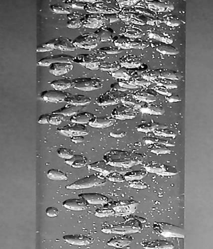
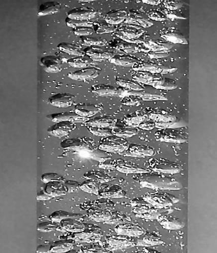
295 Test Conditions: A = 0.62% Open Vent Mode Lower Horizontal Connector 272 U G = 5.0 cm/s U G = 6.0 cm/s U G = 7.0 cm/s U G = 8.0 cm/s U G = 9.0 cm/s U G = 10.0 cm/s U G = 11.0 cm/s U G = 12.0 cm/s U G = 13.0 cm/s

296 Test Conditions: A = 0.62% Open Vent Mode Lower Horizontal Connector 273 U G = 14.0 cm/s U G = 15.0 cm/s U G = 16.0 cm/s U G = 17.0 cm/s U G = 18.0 cm/s U G = 19.0 cm/s

297 Test Conditions: A = 0.62% Closed Vent Mode Lower Horizontal Connector 274 U G = 0.5 cm/s U G = 1.0 cm/s U G = 1.5 cm/s U G = 2.0 cm/s U G = 2.5 cm/s U G = 3.0 cm/s U G = 3.5 cm/s U G = 4.0 cm/s U G = 4.5 cm/s

298 Test Conditions: A = 0.62% Closed Vent Mode Lower Horizontal Connector 275 U G = 5.0 cm/s U G = 6.0 cm/s U G = 7.0 cm/s U G = 8.0 cm/s U G = 9.0 cm/s U G = 10.0 cm/s U G = 11.0 cm/s U G = 12.0 cm/s U G = 13.0 cm/s

299 Test Conditions: A = 0.62% Closed Vent Mode Lower Horizontal Connector 276 U G = 14.0 cm/s U G = 15.0 cm/s U G = 16.0 cm/s U G = 17.0 cm/s U G = 18.0 cm/s U G = 19.0 cm/s

300 Test Conditions: A = 0.99% Open Vent Mode Lower Horizontal Connector 277 U G = 0.5 cm/s U G = 1.0 cm/s U G = 1.5 cm/s U G = 2.0 cm/s U G = 2.5 cm/s U G = 3.0 cm/s U G = 3.5 cm/s U G = 4.0 cm/s U G = 4.5 cm/s

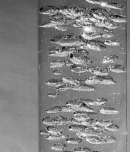
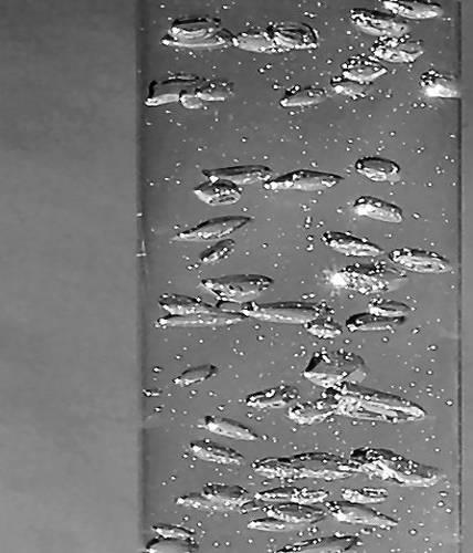
301 Test Conditions: A = 0.99% Open Vent Mode Lower Horizontal Connector 278 U G = 5.0 cm/s U G = 6.0 cm/s U G = 7.0 cm/s U G = 8.0 cm/s U G = 9.0 cm/s U G = 10.0 cm/s U G = 11.0 cm/s U G = 12.0 cm/s U G = 13.0 cm/s

302 Test Conditions: A = 0.99% Open Vent Mode Lower Horizontal Connector 279 U G = 14.0 cm/s U G = 15.0 cm/s U G = 16.0 cm/s U G = 17.0 cm/s U G = 18.0 cm/s U G = 19.0 cm/s

303 Test Conditions: A = 0.99% Closed Vent Mode Lower Horizontal Connector 280 U G = 0.5 cm/s U G = 1.0 cm/s U G = 1.5 cm/s U G = 2.0 cm/s U G = 2.5 cm/s U G = 3.0 cm/s U G = 3.5 cm/s U G = 4.0 cm/s U G = 4.5 cm/s

304 Test Conditions: A = 0.99% Closed Vent Mode Lower Horizontal Connector 281 U G = 5.0 cm/s U G = 6.0 cm/s U G = 7.0 cm/s U G = 8.0 cm/s U G = 9.0 cm/s U G = 10.0 cm/s U G = 11.0 cm/s U G = 12.0 cm/s U G = 13.0 cm/s

305 Test Conditions: A = 0.99% Closed Vent Mode Lower Horizontal Connector 282 U G = 14.0 cm/s U G = 15.0 cm/s U G = 16.0 cm/s U G = 17.0 cm/s U G = 18.0 cm/s U G = 19.0 cm/s

306 Test Conditions: A = 2.22% Open Vent Mode Lower Horizontal Connector 283 U G = 0.5 cm/s U G = 1.0 cm/s U G = 1.5 cm/s U G = 2.0 cm/s U G = 2.5 cm/s U G = 3.0 cm/s U G = 3.5 cm/s U G = 4.0 cm/s U G = 4.5 cm/s

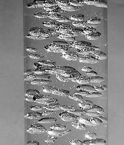
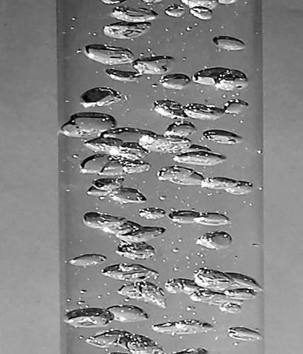
307 Test Conditions: A = 2.22% Open Vent Mode Lower Horizontal Connector 284 U G = 5.0 cm/s U G = 6.0 cm/s U G = 7.0 cm/s U G = 8.0 cm/s U G = 9.0 cm/s U G = 10.0 cm/s U G = 11.0 cm/s U G = 12.0 cm/s U G = 13.0 cm/s

308 Test Conditions: A = 2.22% Open Vent Mode Lower Horizontal Connector 285 U G = 14.0 cm/s U G = 15.0 cm/s U G = 16.0 cm/s U G = 17.0 cm/s U G = 18.0 cm/s U G = 19.0 cm/s

309 Test Conditions: A = 2.22% Closed Vent Mode Lower Horizontal Connector 286 U G = 0.5 cm/s U G = 1.0 cm/s U G = 1.5 cm/s U G = 2.0 cm/s U G = 2.5 cm/s U G = 3.0 cm/s U G = 3.5 cm/s U G = 4.0 cm/s U G = 4.5 cm/s