The Inflow Performance Relationship, or IPR, defines a well s flowing production potential:

Transcription

1 Artificial Lift Methods Artificial Lift Overview INTRODUCTION TO ARTIFICIAL LIFT The Inflow Performance Relationship, or IPR, defines a well s flowing production potential: (1) q = PI (Pavg - Pwf) where q = production rate, B/D PI = productivity index, B/D/psi Pavg, or = average reservoir pressure, psi Pwf = flowing bottomhole pressure, psi (Figure 1) illustrates this relationship for a solution gas drive reservoir. Note that for a given average reservoir pressure and productivity index, P wf determines the well s production potential. The lower the flowing bottomhole pressure, the higher the production rate. The well s maximum or absolute flow potential would correspond to a Pwf of zero. Figure 1

2 A well never actually attains its absolute flow potential, because in order for it to flow, P wf must exceed the backpressure that the producing fluid exerts on the formation as it moves through the production system. This backpressure or bottomhole pressure has the following components: Hydrostatic pressure of the producing fluid column Friction pressure caused by fluid movement through the tubing, wellhead and surface equipment Kinetic or potential losses due to diameter restrictions, pipe bends or elevation changes. In most production systems, these are not of the same magnitude as hydrostatic or friction pressures; in others, however, they may be significant. Artificial lift is a means of overcoming bottomhole pressure so that a well can produce at some desired rate, either by injecting gas into the producing fluid column to reduce its hydrostatic pressure, or using a downhole pump to provide additional lift pressure downhole. We tend to associate artificial lift with mature, depleted fields, where P avg has declined such that the reservoir can no longer produce under its natural energy. But these methods are also used in younger fields to increase production rates and improve project economics. ARTIFICIAL LIFT METHODS The two major categories of artificial lift are gas lift and pump-assisted lift. Plunger lift, which combines elements of both categories, is used primarily in gas and high-gor wells to produce relatively small volumes of liquid. GAS LIFT Gas lift involves injecting high-pressure gas from the surface into the producing fluid column through one or more subsurface valves set at predetermined depths ( Figure 2: Gas lift system. Courtesy Weatherford International Ltd). Figure 2

3 There are two main types of gas lift: Continuous gas lift, where gas is injected in a constant, uninterrupted stream. This lowers the overall density of the fluid column and reduces the hydrostatic component of the flowing bottomhole pressure. Thus, for a given average reservoir pressure and productivity index, the well is able to flow at a higher rate. This method is generally applied to wells with high productivity indexes and high bottomhole pressures relative to their depths. Intermittent gas lift, which is designed for lower-productivity wells. In this type of gas lift installation, a volume of formation fluid accumulates inside the production tubing. A highpressure slug of gas is then injected below the liquid, physically displacing it to the surface. As soon as the fluid is produced, gas injection is interrupted, and the cycle of liquid accumulation-gas injection-liquid production is repeated. The availability of gas and the costs for compression and injection are major considerations in planning a gas lift installation. Where these gas injection requirements can be satisfied, gas lift offers a flexible means of optimizing production. It can be used in deviated or crooked wellbores, and in high-temperature environments that might adversely affect other lift methods, and it is conducive to maximizing lift efficiency in high-gor wells. Wireline-retrievable gas lift valves can be pulled and reinstalled without pulling the tubing, making it relatively easy and economical to modify the design. On the negative side, gas lift system costs can adversely impact profitability if the source gas requires additional processing or surface compression. Lift efficiency can be reduced by corrosion and paraffin, which increase friction and backpressure. Tubing size and surface flowline length also affect system efficiency. Another disadvantage of gas lift is its difficulty in fully depleting lowpressure, low-productivity wells. Also, the start-and-stop nature of intermittent gas lift may cause downhole pressure surges and lead to increased sand production. PUMP-ASSISTED LIFT Downhole pumps are used to increase pressure at the bottom of the tubing string by an amount sufficient to lift fluid to the surface. These pumps fall into two basic categories: positive displacement pumps and dynamic displacement pumps. A positive displacement pump works by moving fluid from a suction chamber to a discharge chamber. The suction chamber volume increases as the discharge chamber volume decreases, causing fluid to enter the suction chamber. As the cycle reverses, the suction volume decreases and the discharge volume increases, forcing the fluid to the discharge end of the pump. This basic operating principle applies to reciprocating rod pumps, hydraulic piston pumps and progressive cavity pumps (PCPs). A dynamic displacement pump works by causing fluid to move from inlet to outlet under its own momentum, as is the case with a centrifugal pump. Dynamic displacement pumps commonly used in artificial lift include electrical submersible pumps (ESPs) and hydraulic jet pumps. Reciprocating Rod Pump Systems A reciprocating rod pump system is made up of the following components ( Figure 3: Rod pumping system. Courtesy Weatherford International Ltd):

4 Figure 3 A beam pumping unit, operated by an electric motor or gas engine. A string of steel or fiberglass sucker rods that connect the beam pumping unit to the downhole pump. A subsurface pump, which consists of a barrel, plunger and valve assembly that moves fluid through the tubing and up to the surface. Beam pumping is the most common and arguably the most recognizable artificial lift method. It can be used for a wide range of production rates and operating conditions, and rod pump systems are relatively simple to operate and maintain. However, the volumetric efficiency (capacity) of a rod pump is lower in wells with high gas-liquid ratios, small tubing diameters or deep producing intervals. Surface equipment requires a large amount of space compared with other lift methods, and its initial installation may involve relatively high capital costs. Progressive Cavity Pump (PCP) Systems A progressive cavity pump consists of a spiral rotor that turns eccentrically inside an elastomerlined stator (Figure 4: PCP system. Courtesy Weatherford International Ltd).

5 Figure 4 As the rotor turns, cavities between the threads of the pump rotor and stator move upward. The rotor is most often powered by rods connected to a motor on the surface, although some assemblies are driven by subsurface electric motors. Progressive cavity pumps are commonly used for dewatering coalbed methane gas wells, for production and injection applications in waterflood projects and for producing heavy or high-solids oil. They are versatile, generally very efficient, and excellent for handling fluids with high solids content. However, because of the torsional stresses placed on rod strings and temperature limitations on the stator elastomers, they are not used in deeper wells. Hydraulic Pump Systems Hydraulic pump systems use a power fluid usually light oil or water that is injected from the surface to operate a downhole pump. Multiple wells can be produced using a single surface power fluid installation (Figure 5: Hydraulic pumping system. Courtesy Weatherford International Ltd).

6 Figure 5 Downhole hydraulic pumps may be either of two types. With a reciprocating hydraulic pump, the injected power fluid operates a downhole fluid engine, which drives a piston to pump formation fluid and spent power fluid to the surface. A jet pump is a type of hydraulic pump with no moving parts. Power fluid is injected into the pump body and into a small-diameter nozzle, where it becomes a low-pressure, highvelocity jet. Formation fluid mixes with the power fluid, and then passes into an expandingdiameter diffuser. This reduces the velocity of the fluid mixture, while causing its pressure to increase to a level that is sufficient to lift it to the surface Hydraulic pumps can be used at depths from 1000 to 17,000 feet and are capable of producing at rates from 100 to 10,000 B/D. They can be hydraulically circulated in and out of the well, thus eliminating the need for wireline or rig operations to replace pumps and making this system adaptable to changing field conditions. Another advantage is that heavy, viscous fluids are easier to lift after mixing with the lighter power fluid. Disadvantages of hydraulic pump systems include the potential fire hazards if oil is used as a power fluid, the difficulty in pumping produced fluids with high solids content, the effects of gas on pump efficiency and the need for dual strings of tubing on some installations. Electrical Submersible Pumps An electric submersible pumping (ESP) assembly consists of a downhole centrifugal pump driven by a submersible electric motor, which is connected to a power source at the surface ( Figure 6: ESP system. Courtesy Weatherford International Ltd).

7 Figure 6 The pump and motor assembly, which may be several hundred feet long, is connected to the surface by an armored cable that provides electric power and control. On a cost-per-barrel basis, ESP systems are among the most efficient and economical of lift methods. Fluid volumes ranging from 100 to 60,000 B/D, including high water-cut fluids, can be handled by ESP systems. These systems can be installed in high-temperature wells (above 350 F) using high-temperature motors and cables. The pumps can be modified to lift corrosive fluids and sand. ESP systems can be used in high-angle and horizontal wells if placed in straight or vertical sections of the well. ESP pumps can be damaged from gas lock. In wells producing high GOR fluids, a downhole gas separator must be installed. Another disadvantage is that ESP pumps have limited production ranges determined by the number and type of pump stages; changing production rates requires either a pump change or installation of a variable-speed surface drive. The tubing must be pulled for pump repairs or replacement. PLUNGER LIFT Plunger lift is the only artificial lift method that relies solely on the well s natural energy to lift fluids. The plunger, traveling inside the tubing, moves upward when the pressure of the gas below it is greater than the pressure of the liquid above it ( Figure 7: Plunger lift system. Courtesy Weatherford International Ltd ).

8 Figure 7 As the plunger travels to the surface, it creates a solid interface between the lifted gas below and produced fluid above to maximize lifting energy. Any gas that bypasses the plunger during the lifting cycle flows up the production tubing and sweeps the area to minimize liquid fallback. Plunger lift provides a cost-effective method of artificial lift that can be used to efficiently produce both gas wells with fluid loads and high GOR oil wells. SELECTING AN ARTIFICIAL LIFT METHOD Artificial lift considerations should ideally be part of the well planning process. Future lift requirements will be based on the overall reservoir exploitation strategy, and will have a strong impact on the well design. INITIAL SCREENING CRITERIA Tables 1 and 2 below summarize some of the key factors that influence the selection of an artificial lift method. Table 1 Reservoir and Hole Considerations in Selecting an Artificial Lift Method (after Brown, 1980) Reservoir Characteristics: IPR A well s inflow performance relationship defines its production potential Liquid production rate The anticipated production rate is a controlling factor in selecting a lift method; positive displacement pumps are generally limited to rates of B/D. Water cut High water cuts require a lift method that can move large volumes of fluid

9 Table 1 Reservoir and Hole Considerations in Selecting an Artificial Lift Method (after Brown, 1980) Reservoir Characteristics: Gas-liquid ratio A high GLR generally lowers the efficiency of pump-assisted lift Viscosity Viscosities less than 10 cp are generally not a factor in selecting a lift method; high-viscosity fluids can cause difficulty, particularly in sucker rod pumping Formation volume factor Ratio of reservoir volume to surface volume determines how much total fluid must be lifted to achieve the desired surface production rate Reservoir drive mechanism Depletion drive reservoirs: Late-stage production may require pumping to produce low fluid volumes or injected water. Water drive reservoirs : High water cuts may cause problems for lifting systems Gas cap drive reservoirs : Increasing gas-liquid ratios may affect lift efficiency. Other reservoir problems Sand, paraffin, or scale can cause plugging and/or abrasion. Presence of H2S, CO2 or salt water can cause corrosion. Downhole emulsions can increase backpressure and reduce lifting efficiency. High bottomhole temperatures can affect downhole equipment. Hole Characteristics: Well depth The well depth dictates how much surface energy is needed to move fluids to surface, and may place limits on sucker rods and other equipment. Completion type Completion and perforation skin factors affect inflow performance. Casing and tubing sizes Small-diameter casing limits the production tubing size and constrains multiple options. Small-diameter tubing will limit production rates, but larger tubing may allow excessive fluid fallback. Wellbore deviation Highly deviated wells may limit applications of beam pumping or PCP systems because of drag, compressive forces and potential for rod and tubing wear. Table 2 Surface and Field Operating Considerations in Selecting an Artificial Lift Method (after Brown, 1980) Surface Characteristics: Flow rates Flow rates are governed by wellhead pressures and backpressures in surface production equipment (i.e., separators, chokes and flowlines).

10 Table 2 Surface and Field Operating Considerations in Selecting an Artificial Lift Method (after Brown, 1980) Surface Characteristics: Flowline size and length Flowline length and diameter determines wellhead pressure requirements and affects the overall performance of the production system. Fluid contaminants Scale, paraffin or salt can increase the backpressure on a well. Power sources The availability of electricity or natural gas governs the type of artificial lift selected. Diesel, propane or other sources may also be considered. Field location In offshore fields, the availability of platform space and placement of directional wells are primary considerations. In onshore fields, such factors as noise limits, safety, environmental, pollution concerns, surface access and well spacing must be considered. Climate and Physical environment Affect the performance of surface equipment. Field Operating Characteristics: Long-range recovery plans Field conditions may change over time. Pressure maintenance operations Water or gas injection may change the artificial lift requirements for a field. Enhanced oil recovery projects EOR processes may change fluid properties and require changes in the artificial lift system. Field automation If the surface control equipment will be electrically powered, an electrically powered artificial lift system should be considered. Availability of operating and service personnel and support services Some artificial lift systems are relatively low-maintenance; others require regular monitoring and adjustment. Servicing requirements (e.g., workover rig versus wireline unit) should be considered. Familiarity of field personnel with equipment should also be taken into account. Clegg, Bucaram and Hein (1993), in a piece written for the SPE Distinguished Author Series, observe that selecting the proper artificial lift method is critical to the long-term profitability of most producing oil and gas wells. They list 31attributes for comparing the eight most common artificial lift techniques (continuous and intermittent gas lift, beam pumping, progressing cavity pumping, hydraulic pumping, electric submersible pumping, jet pumping and plunger lift), and provide practical guidelines for assessing each method s capabilities. These are summarized as follows: Design considerations and overall comparisons: Capital cost Downhole equipment Operating costs Reliability

11 Efficiency Flexibility Salvage value System (total) Miscellaneous [operating] Usage/outlook problems Normal operating considerations: Prime mover flexibility Surveillance Testing Casing size limits Depth limits Intake capabilities Noise level Time cycle and pump-off controllers application Obtrusiveness Artificial lift considerations: Corrosive/scale handling ability Crooked/deviated holes Multiple completions Gas-handling ability Offshore application Paraffin-handling capability Slim-hole completions Solids/sand-handling ability Temperature limitations High-viscosity fluid handling High-volume lift capabilities Low-volume lift capabilities Finally, Table 3 (from Weatherford International Ltd., 2005) summarizes typical characteristics and applications for each form of artificial lift. These are general guidelines, which vary among manufacturers and researchers. Each application needs to be evaluated on a well-by-well basis. Table 3: Artificial Lift Methods Characteristics and Areas of Application (after Weatherford, 2005) Operati ng Parame ters Positive displacement pumps Dynamic displacement pumps ESP Gas lift Plunge r lift 5000 to ft To 8000 ft Rod pump PCP Hydrau lic Piston Hydrau lic Jet Typical Operati ng Depth (TVD) 100 to ft 2000 to 4500 ft 7500 to 5000 to ft ft Maximu m Operati ng Depth (TVD) ft 6000 ft ft ft ft ft ft Typical Operati ng Volume 5 to 1500 BFPD 5 to 2200 BFPD BFPD 100 to BFPD BFPD BFPD 1-5 BFPD Maximu >

12 Table 3: Artificial Lift Methods Characteristics and Areas of Application (after Weatherford, 2005) Operati ng Parame ters Positive displacement pumps Dynamic displacement pumps Gas lift Plunge r lift Rod pump PCP Hydrau lic Piston ESP Hydrau lic Jet m Operati ng Volume BFPD BFPD BFPD BFPD 0 BFPD BFPD BFPD Typical Operati ng Temper ature º F º F º F º F ºF 120 º F [ º C] [24-65 º C] [40120 º C] [40120 º C] [ º C] Maximu m Operati ng tempera ture 550 º F 250 º F 500 º F 400 º F 500 º F 400 º F 500 º F [288 º C] [120 º C] [260 º C] [205 º C] [260 º C] [205 º C] [260 º C] Typical Wellbor e Deviatio n 0-20 deg landed pump N/A 0-20 deg landed pump 0-20 deg hole angle 0-50 deg N/A Maximu m Wellbor e Deviatio n 0-90 deg landed pump 0-90 deg 0-90 deg 0-90 deg 80 deg < 15 deg/10 0 ft < 15 deg/10 0 ft 70 deg, short to medium radius Corrosio n handling Good to Excelle nt Fair Good Good Excelle nt Good to excellent Excelle nt Gas handling Fair to good Good Fair Fair Good Excellent Excelle nt Solids handling Fair to good Excelle nt Poor Fair Good Good Poor to Fair >8º API < 35 º API >8º API > 10 º API >8º API > 15 º API GLR = 300 SCF/B bl per 1000 ft of Fluid gravity 0-90 deg < 24 deg/10 0 ft [50 º C]

13 Table 3: Artificial Lift Methods Characteristics and Areas of Application (after Weatherford, 2005) Operati ng Parame ters Positive displacement pumps Rod pump PCP Hydrau lic Piston Dynamic displacement pumps ESP Gas lift Plunge r lift Hydrau lic Jet depth Servicin g Workov er or pulling rig Workov er or pulling rig Hydrau lic or wirelin e Workov er or pulling rig Hydrau lic or wirelin e Wireline or workover rig Wellhe ad catcher or wireline Prime mover Gas or electric Gas or electric Multicylinde r or electric Electric motor Multicylinde r or electric Compres sor Well s natural energy Offshor e applicati ons Limited Good Good Excelle nt Excelle nt Excellent N/A System efficienc y 45% 60% 40% 70% 45% 55% 35% 60% 10% 30% 10% 30% N/A ECONOMICS OF ARTIFICIAL LIFT The features, benefits and limitations of one artificial lift method are relative to those of the other methods under consideration. Each method should be evaluated from the standpoint of comparative economics. Brown (1980) lists six critical bases of comparison: Initial capital cost Monthly operating expense Equipment life Number of wells to be lifted Surplus equipment availability Expected producing life of well(s) Capital cost considerations may favor one type of system over another, particularly when there is significant uncertainty regarding well performance characteristics or reserve volumes. Gas lift is not likely to be a good option for a one or two-well system, for example particularly if it requires adding surface compression facilities. For multiple wells, however, it may be a very economical choice. Hydraulic pumping is likewise less costly when multiple wells are operated from a central injection facility. Projected operating costs also figure into the selection of an artificial lift method. High gas prices will reduce the profitability of gas lift, particularly if it becomes necessary to purchase additional gas for injection. But gas lift may be an attractive option in a remote field where there is no market

14 for produced gas. In the same way, in places where electricity is not readily available, submersible pumps will be less attractive compared to gas lift or other forms of pump-assisted lift. System reliability and easy access to repair equipment and services must also be considered. Sometimes, the prevalence of a particular type of lift equipment in a given area will make that system more attractive. If a well is expected to have a short producing life, capital and operating costs will play an important role in the overall field economics and will affect the choice of an artificial lift system. It is clear that for each well or field situation, a number of factors will affect the choice of artificial lift system. Equipment manufacturers can explain important advantages and disadvantages of different systems. Each type of artificial lift method has economic and operating limitations that can make it more or less desirable when compared to others. Similarly, one artificial lift system will usually have at least one advantage over all others for a given set of operating conditions. Gas Lift GAS LIFT SYSTEM OVERVIEW Gas lift is a four-step process (Figure 1: Gas lift system): Figure 1 1. Natural gas is compressed at the surface and routed to individual wells. 2. This lift gas is injected downhole and into the produced fluid stream through one or more valves set at specified depths (most commonly, the gas is injected into the production tubing from the casing-tubing annulus). 3. The lift gas and formation fluids are produced to the surface. 4. The gas and liquids are separated; the gas is then treated and sent either to compression or to sales. In most wells, gas is injected continuously into the produced fluid stream. This continuous gas lift process reduces the backpressure on the formation by reducing the density and therefore the hydrostatic pressure of the produced fluid (Figure 2: Continuous gas lift).

15 Figure 2 Continuous gas lift is typically used in higher productivity wells to handle rates ranging from 100 up to 30,000 B/D. In wells with very high productivity indexes, even higher rates can be attained by injecting gas into the tubing and producing fluids through the casing-tubing annulus. Intermittent gas lift employs much of the same equipment as continuous lift, but its operating principle is completely different. Rather than lowering the density of the produced fluid so that it can produce in a continuous flow stream, intermittent lift works by physically displacing slugs of liquid to the surface (Figure 3: Intermittent gas lift):

16 Figure 3 When a certain volume of fluid accumulates in the wellbore, gas is injected into the tubing, where it lifts the column of fluid to the surface as a slug. As each liquid slug is produced, gas injection is interrupted to allow the fluid volume to build up again. Intermittent injection uses a timer or an adjustable choke located on the surface to control the gas injection. Cycling of gas injection is regulated to coincide with the accumulation of wellbore fluids. Intermittent lift is generally used in wells with limited inflow potential (i.e., high productivity index with low average reservoir pressure or, alternatively, low productivity index with high reservoir pressure).

17 As is true for other artificial lift methods, gas lift offers a number of benefits, and at the same time has some inherent limitations (Brown, 1982; Tak ács, 2005). Advantages include: Flexibility in handling a wide range of production rates; can convert from continuous to intermittent lift as reservoir pressure or well productivity declines. Relatively good solids-handling capabilities. Suitability for producing high-glr wells (unlike pump-assisted lift, where gas production is usually detrimental to system efficiency). Can be used in deviated wells Installations can be designed for servicing with wireline units; gas lift valves can be run and retrieved without having to pull tubing string. Relatively low-profile surface wellhead equipment, takes up little surface space. Can easily manage high bottomhole temperatures or corrosive environments Most installations provide full-bore tubing strings, which facilitate downhole surveys, well monitoring and workover. Some of the main limitations and disadvantages of gas lift systems include: Obtaining sufficient amounts of lift gas. The need to provide compression and gas treatment facilities. Generally lower energy efficiency than other lift methods. Cannot reduce bottomhole pressure to the low levels attainable by pump-assisted lift. DOWNHOLE INSTALLATIONS The key subsurface components of a gas lift system are the gas lift valves that regulate the flow of injected gas into the producing fluid column. These pressure-operated devices usually 1 or 1.5 inches in diameter and about 16 to 24 inches long are placed in mandrels that are set at selected depths in the tubing string, most often in a conventional or side pocket configuration (Figure 1: Conventional and side pocket mandrel installations).

18 Figure 1 In a conventional or tubing retrievable valve-mandrel configuration, the valves are run with the tubing string, and the tubing must be pulled in order to repair or replace a valve. (Figure 2) shows a valve designed for a conventional gas lift installation. (Camco conventional injection-pressure operated gas lift valves, Types J50 and J40. Courtesy of Schlumberger.)

19 Figure 2 Side pocket mandrels are designed to accommodate valves in parallel with the tubing (Figure 3: Camco KBMM Series side pocket mandrel. Courtesy of Schlumberger.). These are the most common types of mandrels in use, their main attraction being that they enable gas lift valves to be run and retrieved on wireline. This eliminates the need to pull the tubing for valve repairs or adjustments.

20 Figure 3 INSTALLATION TYPES The type of downhole installation used in a gas lift well depends on whether it is to be placed on continuous or intermittent lift. This in turn depends on its present and anticipated future inflow performance. Other considerations include completion type, casing diameters and wellbore deviation. As is true for any type of downhole installation, a gas lift system should be designed with enough flexibility to minimize the number of workovers required over a well s producing life. Except for the annular flow installation mentioned at the end of this section, all of the downhole installations discussed here are designed for gas injection through the casing and production though the tubing string. OPEN INSTALLATION An open gas lift installation is one in which the tubing string is suspended in the well without a packer, and the casing and tubing are in communication. This, the oldest type of gas lift installation, has several major disadvantages: Only a fluid seal in the annulus prevents gas from blowing around the bottom of the tubing. This results in wasted gas, additional backpressure on the formation, and reduced production rates.

21 Without a packer, the lower gas lift valves may be submerged in well fluids because the fluid rises in the annulus every time the well is shut-in. This may lead to valve corrosion. When production resumes, the fluid must flow back through the gas lift valves, causing the valves to wear out faster. The open installation is not normally recommended, and it is used nowadays only when a packer cannot be installed. SEMI-CLOSED INSTALLATION A semi-closed installation has a packer installed in the tubing to seal off the tubing-casing annulus, as shown in the continuous gas lift well of (Figure 4) (Semi-closed gas lift installation).

22 Figure 4 This is the most common type of installation for continuous gas lift wells. It eliminates most of the characteristic disadvantages of the open installation the packer keeps produced fluids from entering the annulus, and prevents the casing pressure from directly communicating with the formation. This installation is also used in intermittent gas lift wells. It is not the best choice for wells exhibiting very low bottomhole pressures, however, because it is possible that gas injected into the tubing string may place additional backpressure on the formation when the operating valve is open. CLOSED INSTALLATION A closed installation (Figure 5) is similar to a semi-closed installation, except that a standing valve is placed in the tubing string below the bottom gas lift valve to prevent fluids from moving downward. Thus, high-pressure gas injected into the tubing from the annulus cannot increase backpressure on the formation, and any produced fluids standing in the tubing will not flow back into the formation. These features make the closed installation the option of choice for intermittent gas lift.

23 Figure 5 CHAMBER INSTALLATIONS A chamber installation can greatly increase production rates, especially in wells with low bottomhole pressures and high productivity indexes. It is used in intermittent lift operations to increase the volume of fluids in the wellbore prior to lifting, without significantly increasing the backpressure on the formation. One type of chamber installation consists of a lower packer and an upper, or bypass packer. This two-packer chamber installation works as follows: As the chamber fills with fluid, gas in the chamber passes through a bleed valve into the tubing.

24 When the chamber is filled, a slug of gas is injected down the annulus to open the operating valve. The gas in the chamber forces the fluid to enter the tubing through a perforated nipple above the bottom packer (Figure 6: Chamber installation fluid entry). Figure 6 When all the fluid in the chamber above the nipple is forced into the tubing, gas follows behind the slug and forces it to the surface (Figure 7: Chamber installation fluid displacement).

25 Figure 7 The operating valve should close when the slug reaches the surface, at which time the filling cycle begins again. In wells where it is not feasible to set two packers, an insert chamber installation may be used, in which the chamber is formed by a larger-diameter section of pipe at the bottom of the tubing string. The principles of operation are the same as for the two-packer installation. Alternative configurations may be designed for special circumstances. SLIM HOLE INSTALLATIONS

26 Slim hole completions are often used in lower productivity wells. These normally use a string of 23/8 to 3-1/2-inch OD pipe as the production casing. Smaller size tubing, (e.g., 1 to 1-1/2-inches in diameter) is then run inside this casing (Figure 8: Slim hole gas lift completion). Figure 8 Slim hole completions are especially useful for producing from two or more zones without commingling. Production rates for continuous gas lift will depend on the ID of the tubing, but can range from 150 B/D for 3/4-inch tubing to 900 B/D for 1 1/2-inch ID tubing. The rates for intermittent injection in slim hole wells are considerably lower. DUAL INSTALLATIONS Gas lift wells, like flowing wells, can be designed with parallel or concentric dual tubing strings (Figure 9: Dual gas lift installations). The two most common configurations are (1) parallel strings of 2 3/8-inch OD tubing inside 7-inch casing and (2) parallel strings of 3 1/2-inch OD tubing inside 9 5/8-inch casing (API RP 11V8, 2003).

27 Figure 9 Gas is supplied through the tubing-casing annulus, and injected into two separate tubing strings. The zones may be produced using the same type of lift method (i.e., both on continuous or both on intermittent lift), or the two methods may be used in combination (e.g., one zone is on intermittent lift while the other is on continuous lift). For a dual installation to work, the valves must be spaced to prevent interference between the two zones, and selected so that the desired amounts of gas are injected for each zone. COILED TUBING INSTALLATIONS Coiled tubing can be used to convert a flowing well to gas lift without having to pull the main production tubing string, simply by placing conventional gas lift mandrels at the appropriate depths on the coiled tubing string and then running it inside the production tubing. The smaller diameter of the coiled tubing restricts its use to lower-productivity wells. ANNULAR FLOW INSTALLATIONS In most gas lift operations, production is confined to the tubing because of safety issues, regulatory requirements and company operating policies. This is especially true offshore. In some areas, however such as the Middle East, where wells produce at rates up to 80,000 B/D operators use annular flow gas lift. In this process, gas is injected down the tubing and production is from the annulus. A bull plug is placed at the bottom of the tubing to contain the injected gas. A small-bore orifice or check valve can also be used for this purpose.

28 Apart from regulatory prohibitions, annular flow installations are limited in their application due to concerns about casing corrosion, high injection requirements and the potential for fluid slugging as production rates decline. GAS LIFT VALVES Depending on where it is placed in the tubing string, a gas lift valve may be used as an operating valve or an unloading valve. The operating valve is the deepest valve in the string. It is designed and placed to ensure that the proper amount of gas is injected into the tubing at the appropriate depth to optimize well performance. Unloading valves are set are predetermined depths above the operating valve. They are used to progressively reduce the static fluid level in a well when it is first brought on production (or returned to production after having been killed for workover or other operations). As gas is injected into the well, each valve opens in sequence from top to bottom. The gas displaces the liquid in the well, u-tubing it through the unloading valve and displacing it to the surface. As the liquid level drops below the valve, that valve closes and the valve below it opens, and so on down to the operating valve. The unloading valves remain closed during normal production. Individual valve specifications will depend on whether the well is being produced by continuous or intermittent lift. VALVE TYPES Gas lift valves are pressure-operated valves, so-called because they are designed to open or close in response to gas injection pressure, fluid production pressure or both. The pressure that controls the valve operation is that which is exposed to the largest area in the valve. The most common types of gas lift valves are described below: Injection pressure-operated (IPO) valve: Increase in gas injection pressure opens valve; decrease in gas injection pressure closes valve (Figure 1: Camco retrievable injection pressure operated gas lift valves, BK series and R series. Courtesy of Schlumberger.)

29 Figure 1 Production-pressure-operated (PPO) and Differential-pressure-operated valves : Increase in production pressure opens valve; decrease in production pressure closes valve (Figure 2: Camco retrievable production pressure operated gas lift valve, type BKF-12. Courtesy of Schlumberger).

30 Figure 2 Throttling valve: Increase in gas injection pressure opens valve; decrease in gas injection pressure or production pressure closes valve. Combination valves: Increase in production pressure opens valve; decrease in gas injection pressure or production pressure closes valve. Where injection takes place in the annulus and production takes place through the tubing, the gas injection pressure is commonly referred to as the casing pressure and the production pressure is referred to as the tubing pressure. INJECTION PRESSURE-OPERATED VALVES An injection-pressure-operated (IPO) valve opens and closes in response to changes in gas injection pressure. One type of IPO valve, represented schematically in ( Figure 3), operates as follows:

31 Figure 3 The dome is charged to a specified pressure with nitrogen, at a controlled surface temperature. The bellows serve as a flexible or responsive element. Movement of the bellows causes the valve stem to rise and fall, and the ball to open and close over the port. When the port is open, the annulus and tubing are in communication Because the area of the bellows is much larger than the area of the port, and since the bellows is exposed to casing pressure, it is casing pressure that controls the operation of the valve. A buildup in injection pressure opens the valve, and a reduction in injection pressure closes it IPO valves may be classified as either unbalanced or balanced, depending on whether the production pressure plays a role in opening the valve. A balanced valve opens only at a specified pressure and does not respond to pressure changes in the tubing. By design, tubing pressure cannot act on the port or bellows; thus, the valve is not affected by changes in tubing pressure. Only casing pressure can move the bellows and control the flow of gas from the casing into the tubing. An unbalanced valve is one in which the (1) opening or (2) opening and closing pressure are affected by the production pressure. The valve is kept closed by a nitrogen-charged dome that loads the bellows. The bellows is attached to a stem that moves a ball and controls gas flow into the tubing. When tubing pressure is high enough, the ball moves up and the valve opens. The valve in (Figure 1) is unbalanced, since the tubing pressure can open the port. It may also be classified as a single-element valve, since the charge pressure in the dome represents the only control on the valve s operation. In contrast, a double-element valve has two loading elements: the pressure-charged dome and a spring. The spring provides a closing force, which ensures that if the bellows is ruptured, the valve can still close when needed. Double element valves can be used in both continuous and intermittent flow gas lift installations. PRODUCTION PRESSURE-OPERATED VALVES In a production pressure-operated (PPO) valve, the port is exposed to the injection pressure and the bellows is exposed to the production pressure (Figure 4: Production pressure-operated gas lift valve ). Therefore, it is the production pressure that controls the operation of the valve.

32 Figure 4 PPO valves are double element valves, having both a spring and dome (that may or may not be charged) to supply the valve closing force. Most manufacturers of this valve type charge the dome only when high valve-setting pressures require a supplement to the spring force. Another type of production pressure-operated valve is called a differential-pressure-operated valve. This valve opens and closes in response to tubing pressure relative to the casing pressure. It does not have a pressure-charged dome, but has only a spring acting against the stem and ball. THROTTLING VALVES An IPO valve closes only when the casing pressure falls below the dome pressure. If a tapered seat is used, however, then the valve s closing becomes somewhat sensitive to tubing pressure

33 (Figure 5: Throttling gas lift valve). The tapered seat allows the port area to sense the tubing pressure when the valve is open. This type of valve, called a throttling valve, responds to both tubing and casing pressure, even when it is open. Figure 5 If the tubing pressure is lower than the casing pressure, the throttling valve can close even before the casing pressure has dropped to the dome pressure. In fact, a throttling valve will close with a reduction in tubing pressure - even though the casing pressure is held constant. Throttling valves are also known as proportional valves or continuous flow valves. A throttling valve, then, requires a buildup in tubing or casing pressure to open, and a reduction in tubing or casing pressure to close. During continuous gas lift, the injection gas pressure is held constant by a regulator at the surface; as a result, the valve opens and closes only in response to changes in tubing pressure. PILOT VALVES A pilot valve is a variable-spread valve that is used to unload or kick off a well. It has both a small port to control the spread (i.e., the difference between the opening and closing pressures), and a larger port used for more efficient gas flow. This type of valve is often used for intermittent gas lift operations, which benefit from a valve with a large port size while also keeping close control over the spread (Figure 6: Pilot Valve Operation).

34 Figure 6 DOME CHARGE PRESSURE CORRECTIONS A pressure-operated gas lift valve is charged to its specified dome pressure under controlled surface temperature conditions. Its use in a gas lift installation, however, is based on the charge pressure at its setting depth. The surface pressure therefore has to be corrected for changes in temperature and the gas compressibility factor. Brown (Vol. 2a, 1980), Winkler and Smith (1962), Takács (2005) and others have published charts that can be used to determine the nitrogen dome charge pressure at a given downhole temperature. Winkler and Eads (1989) present the following formulas, which incorporate the effects of the deviation factor for nitrogen: For P d < 1238 psi, where P d = dome charge pressure at 60 ºF, psia: Pd = P d + ( P d x 10-7 (P d)2) x (Tvalve - 60) For P d > 1238 psi: Pd = P d + ( P d x 10-7 (P d)2) x (Tvalve - 60) Example: A gas lift valve has a dome charge pressure of 500 psia at a surface temperature of 60 ºF. What is this pressure at the valve setting depth of 6000 ft, where the temperature is equal to 144 ºF? Solution: P d = 500 psia; P d < 1238 psi Pd = P d + ( P d x 10-7 (P d)2) x (Tvalve - 60) Pd = 500+ ( (500) x 10-7 (500)2) x (144-60) Pd = 587 psi GAS LIFT VALVE SELECTION

35 The type of gas lift valve used in a given installation will depend on whether the well will be placed on continuous or intermittent lift. Some types of valves are suitable for either continuous or intermittent injection; these may be worth considering if the lift method has not been determined or if well performance is marginal. CONTINUOUS GAS LIFT The ideal continuous lift installation would be one in which gas is injected in a steady stream, resulting in more-or-less constant pressures and production rates according to the original design. In reality, production rates and pressures fluctuate from the design parameters, often on a day-today basis. The operating valve thus needs to be sensitive to production pressure when it is in the open position. As production pressure decreases, (i.e., tubing pressure for a tubing installation) the valve should begin to throttle closed to decrease gas throughput; as it increases, the valve should open to increase gas throughput. This proportional response maintains the established flowing wellhead pressure and keeps a constant pressure inside the tubing. Therefore, the best type of operating valve to use for continuous gas flow would be a throttling valve or one with identical gas throughput characteristics. INTERMITTENT GAS LIFT Operating valves used for intermittent lift must be designed for immediate or snap opening and closing. Immediate opening ensures that the gas is injected as a compressed slug and not as a gradual stream that bubbles up through the liquid, while quick valve closure prevents excess gas from being injected. Because the operating valve must be able to handle a relatively large volume of gas in a short time, it has to be able to open to a large port (normally between 3/8 and 3/4 inch), and remain fully open until closing. At the same time, the valve should have a small enough spread so that the volume of gas injected can be tightly controlled. In a single-point injection system, these requirements can be met by using a pilot valve. In a multipoint system, a number of valves are installed at various depths in the tubing string. At each depth, the valve should allow sufficient gas to enter the tubing so that the fluid slug can be moved upward to the next higher valve. As the fluid slug passes by each valve, the pressure under the slug opens that valve, allowing more gas to be injected and supplementing the gas that has entered through the deeper valves. The valves normally remain open until the slug is produced to the surface. GAS LIFT VALVE MECHANICS The opening and closing characteristics of gas lift valves are important considerations in system design and operation. It is important, therefore, to know how and when a valve opens and closes, and to understand the significance of its spread, or difference between opening and closing pressures. PRESSURES TO OPERATE A VALVE Consider an unbalanced IPO single-element valve in the closed position, represented schematically in (Figure 1).

36 Figure 1 To calculate the valve s opening and closing pressures, it is necessary to solve a force-balance equation. The force tending to close the valve, Fclose, is Fclose = P d A b Where P d is the dome charge pressure, and A b is the bellows area. The force tending to open the valve, Fopen, equals Fopen = Pinj (Ab - Ap) + Pprod Ap where Pinj is the injection pressure, Ap is the area of the stem or port; and Pprod is the production pressure. (1) (2)

37 If we set Fclose = Fopen, and define R = (Ap/Ab), we obtain an expression for the injection pressure required to just open the valve at the valve setting depth, or (Pinj)open: (3) Example: Determine the casing (injection) pressure required to open an IPO valve under the following conditions: Bellows area = 0.77 square inches; Port area = square inches; Bellows pressure (corrected to valve depth) = 500 psi; Tubing pressure = 425 psi. Solution: R = A p/a b = 0.129/0.77 = The casing pressure required to open the valve is 515 psi, or 15 psi above the bellows pressure. A higher casing pressure is required because of the effect of the lower tubing pressure on the port area. We may also calculate the pressure required to close the valve once it is opened. Once again, equate the forces tending to keep the valve opened with those tending to close it. The force tending to close the valve is equal to: Fclose = P d A b (1) The force tending to hold the valve open is equal to: Fopen = P inj(a b - A p) + P inj A p (4) Note that when the valve is open, the injection pressure has replaced the production pressure from Equation 2. Equating these two terms yields the casing pressure required to close the valve: (Pinj)close = P d (5) In this example, the bellows pressure is 500 psi, and so the valve will close at this pressure. VALVE SPREAD The difference between the opening pressure and the closing pressure is the spread. Spread = (Pinj)open - (Pinj)close. ) (6) Thus, in the preceding example, the valve spread is ( ) = 15 psi. An inspection of Equations 3 and 5 shows that the spread is a function of the ratio R, the bellows pressure, and the tubing pressure: Spread = (7)

38 For specific bellows and tubing pressures, and since R = (A p/ab), reducing the area of the port will result in lowering the spread. Spread is a particularly important consideration in intermittent lift, because it controls the volume of gas used in each injection cycle. As the spread needed to close the operating valve increases, the amount of gas injected during the cycle also increases this would call for a smaller spread in order to reduce gas volume requirements, and therefore a smaller port size. On the other hand, a smaller port size increases the compression horsepower requirements. Thus, there needs to be a balance between the need to conserve gas and the need to minimize power costs. TEST RACK OPENING PRESSURE (TRO) When unbalanced gas lift valves are tested at the surface, they are set in special valve testers, usually at a production pressure of zero. The injection pressure required to open the valve under these conditions is referred to as the test rack opening, or TRO pressure: (7) where Pd is the dome charge pressure at surface conditions. PRODUCTION PRESSURE EFFECT (PPE) The Production Pressure Effect (PPE) describes the contribution that the production pressure makes to the valve s opening injection pressure, and is equal to the difference between the opening pressure at Pprod = 0 and its actual opening pressure: (8) For a given valve size and port diameter, R is constant, and so PPE increases linearly with production pressure. The slope of this line is known as the Production Pressure Effect Factor (PPEF) and is equal to R/(1-R), or (9) Thus, as valve port sizes increase for a given bellows area, so does the PPEF. FLOW CHARACTERISTICS OF A GAS LIFT VALVE A plot of flow rate versus tubing pressure provides insight into the flow characteristics of a gas lift valve. (Figure 2), for example, illustrates the performance characteristics of a throttling valve (note that in this plot, the vertical axis represents flow rate and the horizontal axis represents tubing pressure ).

39 Figure 2 At very low tubing pressure, to the left of point 1, the valve is closed. As the tubing pressure reaches point 1, the valve begins to open and gas flows from the casing to the tubing. The flow rate increases as the port continues to open. Throttling occurs from point 2 to point 3, at which time the port is fully opened and throttling ends. The maximum flow rate occurs at point 4. As the tubing pressure increases from point 4 to point 5, the tubing and casing pressures become balanced and the flow rate drops to zero. During the reverse cycle (i.e., as the tubing pressure decreases) the valve opens at point 5, throttling takes place between points 3 and 2, and the valve throttle closes between points 2 and 1. CONTINUOUS GAS LIFT In continuous gas lift, an uninterrupted stream of high-pressure gas is injected downhole to reduce the flowing bottomhole pressure of the producing fluid. Injection takes place at set rates and at pre-determined depths to optimize well performance and maximize system efficiency. In most wells, gas is injected down the casing-tubing annulus and into the production tubing.

40 Continuous gas lift works as an artificial lift method because it reduces the hydrostatic component of the bottomhole pressure. As a simple illustration, consider three shut-in wells: Well 1 Well 2 Well ft 6000 ft 6000 ft 2100 psi 2100 psi 2100 psi Fluid in tubing (TVD to surface): Salt water Oil Gas Average fluid gradient: psi/ft psi/ft psi/ft 2790 psi 2076 psi 414 psi True vertical depth (TVD): Average reservoir pressure: Bottomhole pressure at TVD: Note how much lower the bottomhole pressure is in Well 3, and remember the equation that describes the Inflow Performance Relationship: q = PI (Pavg - Pwf) (1) where q = flow rate, PI = productivity index, Pavg = average reservoir pressure and Pwf = flowing bottomhole pressure. Clearly, if we have a well filled with liquid and can mix the liquid column with gas, we can significantly reduce Pwf and, for a given reservoir pressure, increase the inflow from the formation. GAS LIFT VERSUS PUMP-ASSISTED LIFT One of the most basic decisions in selecting an artificial lift method is the choice between gas lift and pump-assisted lift. If we are thinking about installing continuous gas lift, we first must consider the physical limit gas-liquid ratio (GLR) and the optimal GLR. PHYSICAL LIMIT GLR The higher the rate of lift gas injection, the more we improve well performance up to a point. Consider the pressure traverse curves of (Figure 1). These curves were generated for a specified set of flowing well conditions at a tubing depth of 4000 ft.

41 Figure 1 We can see from this figure that: Adding gas to the liquid column lowers the hydrostatic pressure in the wellbore. In this case, increasing the GLR from zero to 100 SCF/Bbl reduces the bottomhole pressure by nearly 600 psi. Higher GLRs result in higher friction pressure losses, which offset the hydrostatic pressure drop. For example, if we again increase the GLR this time from 100 to 200 SCF/Bbl the bottomhole pressure decreases by only 270 psi. As we further increase the GLR, the corresponding bottomhole pressure decrease is smaller still. Eventually, we reach a physical limit GLR where the increase in friction pressure becomes approximately equal to the decrease in hydrostatic pressure. The net change in bottomhole pressure becomes negligible. In (Figure 1), this occurs between 800 and 1000 SCF/Bbl. At this point, injecting additional gas will not result in additional liquid production. The bottomhole pressure corresponding to the physical limit GLR is likely to be much higher than the bottomhole pressure we could attain by installing a downhole pump. This consideration alone would tend to favor pump-assisted lift. But there are other factors to take into account. If a formation is subject to drawdown-related production problems such as water coning or sand production, for instance, then gas lift may be the preferred option.

42 OPTIMAL GLR The choice between gas lift and pump-assisted lift ultimately comes down to economics. Back when the costs of gas re-injection were insignificant compared with the benefits of increasing the incremental oil production rate, the physical limit GLR was considered optimal for meeting gas lift requirements. Since that time, however, with production costs escalating and natural gas becoming valuable in its own right, this is no longer a safe assumption. The actual optimum will be the GLR above which the incremental cost of injecting additional gas exceeds the incremental revenue from increased oil production. This may be lower than the physical limit value. GENERAL DESIGN CONSIDERATIONS Continuous gas lift design follows a systems analysis approach, in which pressures at various key points are determined for the desired production rate and different GLR values. The sequences of steps may vary, depending on which system parameters are known, and which are to be determined. The two most fundamental design issues are How much gas to inject? At what depth(s) to inject it? To address these issues, we must be able to determine how a well is likely to perform under different operating conditions. FORMATION DELIVERABILITY A well s IPR defines the rate at which the formation can deliver fluid to the wellbore under a given reservoir pressure drawdown. This relationship should be established for the current reservoir pressure and, if necessary, for anticipated future reservoir pressures. We can then use the IPR to determine what flowing bottomhole pressure is needed to maintain a desired production rate. The flowing bottomhole pressure attainable from continuous gas lift may be constrained by the formation s tendency toward drawdown-sensitive problems such as sand production and water or gas coning. In any case, it will be restricted to some minimum value by the physical limit GLR (or, if it is lower, the optimal GLR) as described above. The limiting GLR, in turn, will be influenced by the tubing head pressure required to deliver fluid from the wellhead to the separator, and on the pressure losses that take place in the production tubing. As the average reservoir pressure decreases over time, so will the gas injection pressure required to produce at a given flow rate. This effect must be included in the gas lift system design. Likewise, the system must accommodate increases or decreases in GLR or water cut. If we can determine the magnitude of these changes, we must include them in our system design. If not, it may be necessary to adjust the design or rely on subsequent wireline operations to modify valve setting and placement. TUBING HEAD PRESSURE REQUIREMENTS The separator typically represents the downstream end of the production system. To determine the flowing tubing pressure (FTP) needed for formation fluids and lift gas to flow to the separator, we start with the known separator pressure and calculate the pressure losses that occur in the gathering lines at the surface, between the separator and the wellhead. TUBING DIAMETER In most areas, safety and environmental regulations require that fluid be produced through the tubing. In some fields with high-rate producing wells, however, annular production may be an option.

43 (Figure 2) illustrates the difference in production performance for a specific well, based on the size of the production tubing or tubing/casing annulus. The producing GLR is 400 SCF/Bbl, the flowing tubing head pressure is fixed at 250 psi and the well's IPR has been calculated. We consider four different production tubing installations: 1. Tubular flow through 2-inch tubing 2. Tubular flow through 2 1/2-inch tubing 3. Annular flow through 2 x 4 1/2- tubing-casing diameters 4. Annular flow through 2 1/2 x 5 1/2-inch tubing-casing diameters Figure 2 For each curve, a higher flow rate results in a higher bottomhole pressure, and the performance curves shift to the right with increases in the cross-sectional area available for flow. This means that for a given bottomhole pressure, there is a significant flow rate increase with increasing tubing diameter. The intersection of each tubing performance curve with the IPR curve specifies the maximum production rate for the given GLR and surface tubing pressure. (If the desired production rate is lower than this value, it is possible to use smaller production tubing with a performance curve that intersects the IPR curve at a higher bottomhole pressure.) In this example, the highest production rates would be attained through annular flow. GAS INJECTION RATE

44 The gas injection rate frequired for continuous gas lift is estimated as follows: (qgas)inj = 0.001x (GLR2 -GLR1)qliquid (2) where (qgas)inj = gas injection rate, MCF/D GLR2 = producing gas-liquid ratio above the point of gas injection, SCF/Bbl GLR1 = natural producing gas-liquid ratio (i.e., below the point of gas injection), SCF/Bbl qliquid = desired liquid production rate, B/D For example, assume that a well's IPR and pressure traverse relationships indicate that it can produce 850 B/D of fluid at a GLR of 1490 SCF/Bbl, and that the formation GLR is 452 SCF/Bbl. The required gas injection rate would be (qgas)inj = x ( )850 = MCF/D A preliminary step in any gas lift system design is to inventory current and anticipated future gas volumes. The injection gas will probably come from field production operations (usually from a high-pressure separator). Additional makeup gas may be available from local gathering systems or pipelines. GAS INJECTION PRESSURE The surface gas injection pressure that the system requires will depend on the gas lift design parameters for individual wells, including the expected production rates, gas lift GLRs and the depths of the operating valves. Keep in mind that increasing the producing GLR increases flowline pressure losses and can affect separator performance. Gas injection pressure requirements are based on the injection pressure required to open the operating valve. This pressure is greater than the surface injection pressure by an amount equal to the gas gradient times the injection depth. For a tubing installation under static conditions, we may express the pressure gradient in the tubing-casing annulus as (3) where (Pinj)valve is the injection pressure at the operating valve, (Pinj)surf is the minimum operating injection pressure at surface D is the valve depth We may obtain this gradient using the following equation, which is based on a mechanical energy balance and the real gas law (Economides et. al, 1994): (4) where = gas gravity (air = 1) zavg = compressibility factor at average temperature and pressure Tavg = average temperature, ºR = ºF +460 Because the compressibility factor depends on pressure and temperature, we must use an iterative procedure to determine the unknown pressure. Where the casing pressure at the injection point is known, we may obtain (Pinj) surf by trial-and-error as follows: 1. Assume values for (Pinj) surf and zavg at an arithmetic average pressure. 2. Use this value of zavg to calculate a new (Pinj) surf value from Equation Repeat steps 1 and 2 until the values of (Pinj) surf and zavg remain consistent within an acceptable margin.

45 (This same procedure applies if (Pinj) valve is the unknown quantity and (Pinj) surf is known) Gilbert (1954) introduced a simple approximation for Equation 3, in which he assumed = 0.7, zavg = 0.9 and T = 600ºR, and then applied a a Taylor Series expansion: (5) An existing compressor, a high-pressure separator or gas from outside sources may provide sufficient pressure for gas injection. If not, then the system design will have to be based on the surface pressure that is available, or additional compression capabilities will have to be built into the system. LOCATION AND DESIGN OF THE OPERATING VALVE In a tubing installation, lift gas from the surface enters the production tubing through the operating valve. The operating valve is placed such that the gas injection pressure at the valve depth, minus the pressure differential across the valve, is equal to the flowing production pressure at that depth. Depending on the gas lift GLR, we can place the operating valve at any of several depths. It requires less compression horsepower to inject gas at a high pressure and low rate than it does to inject it at a low pressure and high rate. Thus, a gas lift design operating at a low GLR requires a higher operating pressure and a lower compression horsepower. By selecting the lowest operating GLR, we can minimize the horsepower and gas volume requirements for a given production rate. If the available gas volumes or injection pressures are limited, that limitation should be considered in the design. If, on the other hand, we are constrained only by the physical limit GLR, then our design recommendations will be governed by the above guidelines and by the economics of gas injection. The design of the operating valve depends on the type of operation and any anticipated fluctuation in flow rate, producing GLR and water cut. To provide a constant GLR when there are varying production rates, the operating valve should exhibit the gas throughput characteristics of a throttling valve. The capability to adjust the valve through wireline operations allows modification of the design to accommodate changing conditions. Tubing diameters should be specified to give the lowest operating GLR for the target production rate. This will minimize horsepower requirements, surface operating pressure, and the volume of injected gas. SYSTEM DESIGN EXAMPLE Consider a well for which we want to establish a production rate of 600 B/D, and for which we have the following information: Depth: 5600 ft to midpoint of perforations (MPP) Average reservoir pressure = 1750 psi at MPP Target production rate = 600 B/D (32 º API oil; 20% water cut) Formation (current) GLR = 180 SCF/Bbl Pwf required for target rate = 914 psi, based on IPR analysis Average reservoir temperature = 147 ºF Average surface temperature = 65 ºF Tubing size: 2 3/8 inch OD Required tubing head pressure: 100 psi Assume a pressure differential of 100 psi across the operating valve

46 DESIGN OBJECTIVE We want to incorporate this well into an existing gas lift system. The injection line pressure is 800 psi, and the injection pressure available at the wellhead will be 750 psi. Our goal at this stage of the design is to determine (1) the depth of the operating valve and (2) the required gas injection volume. The operating valve should be placed to minimize the gas injection volumes and compression horsepower requirements. This means that we will want to inject at the maximum available pressure of 750 psi. DESIGN PROCEDURE The basic design procedure is adapted from Brown (1980, vol. 2a). Pressure Traverse Using an appropriate multi-phase vertical flow correlation in this case, a spreadsheet-generated model based on a modified Hagedorn-Brown correlation (Economides et. al, 1994) and starting at bottom with the 914 psi required to produce 600 B/D at a GLR of 180 SCF/Bbl, we establish the pressure traverse relationship for the current well conditions ( Figure 3: Pressure traverse curve for example well, 600 B/D at 180 SCF/Bbl GLR). Figure 3

47 In this well, the pressure in the tubing goes to zero before it reaches the surface. In other words, the well cannot produce at the desired rate of 600 B/D under natural flowing conditions. This well is a candidate for gas lift. Gas Gradient and Operating Valve Depth Using Equation 4 and the iterative procedure described above, we can generate the gas injection gradient in the casing-tubing annulus (Figure 4: Gas injection gradient for example well, surface injection pressure of 750 psi). Figure 4 The depth at which the gas injection pressure is equal to the tubing pressure is referred to as the point of balance. It is represented graphically by the intersection of the pressure traverse curve and the gas injection gradient; in this example, the point of balance is at 5372 ft. To account for the 100 psi pressure differential across the operating valve, the valve needs to be set above the point of balance. The setting depth is represented graphically by the intersection of: the tubing pressure traverse curve for GLR = 180 SCF/Bbl, and a line parallel to the gas gradient curve and separated by 100 psi.

48 The depth at which these intersect is 4940 ft (Figure 5: Determination of gas injection point for example well). This is the lowest depth at which we can place the operating valve. Figure 5 Alternatively, we could determine the operating valve depth by generating pressure traverse curves for a set of gas lift GLRs ranging from just above the current 180 SCF/Bbl to the physical limit GLR. For each gas lift GLR, the point of injection would be the depth at which its pressure traverse intersected the curve for the current GLR in other words, where the tubing pressure above the injection point equals the tubing pressure below the injection point In this case, because our design objective is to minimize the gas injection volume and compressor horsepower requirements at a given injection pressure, we are using the gas injection gradient to define the location of the operating valve. Gas Injection Rate To determine the gas injection rate, we must find a GLR for which the pressure traverse fits these two endpoints: The flowing bottomhole pressure at the injection point of 4940 ft The flowing tubing pressure of 100 psi. Using a spreadsheet-based, trial-and-error calculation, we determine that the optimal GLR is 500 SCF/Bbl (Figure 6: Determination of optimal gas lift GLR for example well). Thus, the GLR will be 500 SCF/Bbl above the injection point, and 180 SCF/Bbl below the injection point.

49 Figure 6 From Equation 2, we can now determine the gas injection rate as (qgas)inj = 0.001( )600 = 192 MCF/D Again, this gas lift installation could have been designed for a higher GLR and a lower injection pressure, in which case the operating valve would have been set at a shallower depth. Selecting a lower GLR, however, fits in with our stated design objective for an established gas injection pressure. Production Rate Variations The gas lift valve, located at the injection point, must have a large enough opening to handle the required gas volume at a casing-tubing pressure differential of 100 psi. But what would happen if the flow rate dropped from 600 B/D to 300 B/D? Assuming critical flow conditions, a fixed-size orifice valve would allow the same volume of injection gas to flow for each production rate. Therefore, the GLR at the 300 B/D rate would be too high, resulting in inefficient fluid production. Alternatively, if the production rate was to increase from 600 B/D to 900 B/D for example, following a successful well stimulation treatment the fixed-size orifice valve would be too small to deliver enough gas to the fluid column. When variable production rates are possible, a gas lift valve must be able to respond to these variations while delivering sufficient gas to provide a constant GLR. Where the inflow performance is expected to change over time, a throttling valve may be used to allow a proportional response to flow rate. If this type of valve is used, it should be dynamically performance-tested before installation, to ensure that that the desired gas flow rates at the various

50 casing and tubing pressures will actually occur. The flow testing of valves is often carried out at the manufacturer's shop under simulated operating conditions. The throttling valve, however, does have certain disadvantages: Because throttling valves have limited gas throughput capacity, high-volume wells sometimes require an additional valve to reach the desired lift depth. Pressure adjustments are more difficult than with certain other types of gas lift valves Since more information must be considered, throttling valve designs are more technically detailed and thus require a higher degree of accuracy. UNLOADING IN CONTINUOUS GAS LIFT WELLS Unloading or kicking off is the process of removing a static column of liquid from a wellbore so that the well can flow. A well must be unloaded when either of two conditions occurs: Liquid has accumulated in the well and the fluid level has reached a static point below the surface. The well is full of kill fluid following completion or workover operations, and is ready to be put on production. In either case, the well will not produce until it is unloaded. This unloading process must be part of the gas lift design. In completion and workover operations, we typically unload wells by swabbing, injecting nitrogen or circulating a fluid of lower density than the kill fluid. In continuous gas lift, we assume that the gas injection rate and pressure used to produce the well is available for unloading (in some facilities, an additional kick-off pressure may be available); all that will be needed are additional valves in the tubing, spaced at appropriate depths for unloading fluids. Because of the hydrostatic pressure that the kill fluid exerts in the tubing-casing annulus, the operating valve is open, and the fluid levels in the casing and tubing are equal prior to unloading. Normal practice for unloading gas lift wells is to set the top unloading valve just above the static fluid level. Because most wells that produce on continuous gas lift have relatively high formation pressures, their static fluid levels tend to be at or near the surface. For design purposes, therefore, we may assume that the fluid column reaches to surface. If the density of the wellbore fluid is known, then that value should be used to determine the unloading pressure gradient. If the fluid density is unknown, assume that its gradient is slightly higher than a fresh water gradient of psi/ft psi/ft is a good value for design purposes. GENERAL PRINCIPLES Unloading calculations are based on providing sufficient pressure at progressively lower valve depths to U-tube liquids to the surface, through each valve in succession from top to bottom. To illustrate how the process works, consider a gas lift well with three valves in the tubing string. From top to bottom, these are Valve 1 (unloading valve) Valve 2 (unloading valve) Valve 3 (operating valve) Before unloading, the static fluid level is at the surface, and all valves are open. Unloading takes place according to the following sequence:

51 1. Gas is injected into the annulus at the unloading pressure. The gas displaces the liquid in the annulus through the open valves and into the tubing. The liquid is u-tubed to the surface. 2. As liquid is displaced, the fluid level in the annulus drops until Valve 1 is uncovered. 3. Gas begins to flow into the tubing through Valve 1, reducing the liquid density in the tubing above the point of injection and decreasing the tubing pressure. 4. Because Valves 2 and 3 are still open, the annular fluid level continues to drop as gas is injected through Valve 1 and the pressure in the tubing decreases. 5. The tubing pressure drops to a stable value as the annular fluid level reaches a corresponding stable depth. If the unloading string is properly designed, this stable fluid level should be just below Valve Valve 1 should close just as gas begins to flow through Valve 2. This makes Valve 2 the sole point of gas injection. 7. As gas is injected through Valve 2, the density of the liquid in the tubing above Valve 2 is reduced. The tubing pressure decreases, and the liquid level in the annulus falls because Valve 3 is still open. 8. The tubing pressure drops to a stable value as the annular fluid level reaches a corresponding stable depth. If the unloading string is properly designed, this stable fluid level should be just deep enough to uncover Valve At this point, Valve 2 closes and Valve 3, the operating valve, becomes the sole point of gas injection. UNLOADING DESIGN PROCEDURES The basic objective in designing an unloading string is to progressively transfer the point of gas injection downhole, from the top to the bottom unloading valves, and finally to the operating valve. Each valve closes in turn as the next deepest valve is uncovered, and all of the valves above the operating valve remain closed during normal production. Beyond these general considerations, design procedures vary according to the valve type and to the completeness and reliability of the design input data. Takács (2005) describes several representative valve spacing methods developed for various types of valves. These include procedures for: Injection pressure-operated (IPO) valves: o Variable pressure drop per valve (Winkler and Smith, 1962) o Constant pressure drop per valve (API RP 11V6, 1999) o Constant surface opening pressure (U.S. Industries, 1959) Balanced valves Production pressure-operated valves Throttling valves The design example that follows is based on using IPO valves with constant surface opening pressures. In this procedure, the top-to-bottom injection transfer is accomplished by increasing the production (i.e., tubing) pressures (U.S. Industries, 1959). SYSTEM DESIGN EXAMPLE Table 1 summarizes the design parameters that have been established for a well to be placed on continuous gas lift. Table 1: System Design Example Continuous Gas Lift Average reservoir pressure 1750 psi at midpoint of perforations (5600 ft)

52 Pwf required for target rate 914 psi, based on IPR analysis Target production rate 600 B/D (32 º API oil, water cut = 20 percent ) Average reservoir temperature 147 ºF Average surface temperature 65 ºF Formation GLR 180 SCF/Bbl Tubing: 2 3/8 inch Flowing tubing pressure (FTP) 100 psi Gas lift GLR 500 SCF/Bbl Gas injection rate 192 MCF/D Depth of operating valve 4940 ft Tubing pressure at operating valve depth 744 psi Kill fluid Lease crude oil, kill gradient = 0.38 psi/ft; assume fluid to surface. Formation overbalance = 378 psi As a starting point, we refer to (Figure 6). This shows the gas injection and design gradients for this well, along with the pressure traverse curve above and below the point of injection.

53 Figure 6 For design safety, and to minimize valve interference, it is typical to select a surface design pressure that is the greater of these two values: FTP psi, or FTP x (Injection pressure) In this example, the larger of these values is (0.2 x 750) = 250 psi. Using this surface design pressure and the tubing pressure at the operating valve depth, we can generate a tubing design pressure gradient as shown in (Figure 7). Figure 7 The depth to the top unloading valve (D1) may be calculated using the relationship (1) where (Pinj) = gas injection pressure, psi FTP = flowing tubing pressure, psi

54 kill = kill fluid gradient, psi/ft g = average gas gradient, psi/ft in this example, the average gas gradient is estimated at psi/ft. In this case, This result may also be obtained graphically by starting from the FTP and generating a line parallel to the kill fluid gradient. The depth at which this line intersects the gas injection pressure gradient curve corresponds to D1. From the tubing design gradient line, we determine that the tubing design pressure at this depth is 430 psi. (Figure 8: Unloading design location of top unloading valve.) Figure 8 The tubing design pressure at D1 represents the starting point for locating the second and subsequent valves. Again, we use the pressure gradient of the kill fluid to determine the required gas design pressure. (Figure 9) illustrates the process graphically.

55 Figure 9 For this example, five unloading valves are needed to unload the well, along with the operating valve to provide continuous gas lift operations: Valve No. Depth ft ft ft ft ft

56 6 (Operating valve) 4940 ft There are a number of design options for locating the unloading valves, especially when considering the available selection of valves and the ability to specify the valve opening and closing pressures. Often, for example, a lower valve will be opened before an upper valve is closed in order to provide a smoother unloading operation. CONTINUOUS GAS LIFT: SUMMARY DESIGN PROCEDURE Below is a summary design procedure for a continuous gas lift installation. Depending on the design program in use, certain of these steps will be carried out automatically once the input parameters are entered. Also, the sequence of steps may vary depending on which design parameters (e.g., surface injection pressure, maximum gas volumes, etc.), if any, are already defined. 1. Collect all available input data; Table 1 provides a starting point for listing input parameters. Table 1: Input Data for Continuous Gas Lift Design Well number, field, location, zone Casing data Average reservoir pressure Tubing and production equipment data Average bottomhole, surface temperatures Directional profile Anticipated pressure decline rate Perforation density, diameter Back pressure or separator pressure Sand control equipment Gas-oil ratio, water cut Current gas lift configuration (for existing installations) Gas specific gravity, oil API gravity Available gas injection rate, surface injection pressure (for existing surface facilities) Water specific gravity Kill fluid density Type of well completion Preferred correlations for vertical flow Depths of perforations Preferred correlations for surface flow Establish the well s Inflow Performance Relationship for the current reservoir pressure and, if desired, anticipated future reservoir pressures. 4. Carry out a production system analysis to define pressure traverse curves for various combinations of producing GLR and production tubing assemblies. For each combination, generate the pressure traverse by evaluating the lift performance in the tubing string and the flowing tubing head pressure needed to move fluid from the wellhead to the production separator. For analysis purposes, the range of tubing diameters is based on the diameter of the production casing and/or the type of completion (if annular flow is permitted, consider it as a design option)

57 the lower GLR limit is the formation GLR, while the upper GLR limit is the physical limit GLR above which additional gas injection will not increase the well s production rate. Combine these pressure traverse calculations with the IPR to establish the optimal production rate. For the selected tubing or annular flow system, determine the depths at which the pressure traverse curves for various values of gas lift GLR intersect the pressure traverse curve that corresponds to the well s natural flow. These intersections define several possible locations for the operating valve. Select the depth for the operating valve, keeping in mind that the lowest GLR requires the highest operating pressure, the lowest injected gas volume and lowest compression horsepower. This would normally be the option selected. Determine the injection pressure as a function of depth. At the operating valve, this pressure will be equal to the required production pressure at that depth plus the pressure corresponding to the valve spread. With this pressure as a starting point, obtain the gas gradient in a static gas column using the equation below or a suitable approximation or correlation: where: (Pinj)valve is the injection pressure at the operating valve, psia (Pinj)surf is the minimum operating injection pressure at surface, psia g = gas gravity (air = 1) h = operating valve depth, feet zavg = compressibility factor at average temperature and pressure Tavg = average temperature, ºR Note: Where the lift system is being designed from the bottom up, and (Pinj)valve has been determined, this equation is used to determine the minimum required gas injection pressure at the surface. For an existing gas lift system, where (Pinj)surf is already established, this relationship will be used to determine (Pinj)valve j for various depths. 9. Locate the unloading valves using the appropriate procedure for given valve types and operating conditions. 10. Review the manufacturer s specifications to select the unloading and operating valves that will satisfy the system design for the life of the well. The values are set to meet the required operating conditions. 11. Before completing the system design, be sure there is sufficient gas volume and pressure to meet operating conditions and, finally, be sure that the design can be modified as inflow performance characteristics change. A gas lift system designer must realize that the design is not static. The inflow performance, producing GLR and water cut of the well will probably change as production from the well continues. Also, a system is often designed for an entire field rather than a single well. The future performance of individual wells that collectively make up the system must be considered when developing the optimal field design. INTERMITTENT GAS LIFT Intermittent gas lift is similar to continuous gas lift in that it employs some of the same equipment and procedures, and it improves well performance through the injection of pressurized gas from the surface into the production tubing. The way in which it works, however, is very different. Continuous gas lift is based on introducing a constant stream of gas into the producing fluid column in order to reduce its density.

58 Intermittent lift, on the other hand, is based on periodically injecting slugs of compressed gas below the liquid that accumulates in the production tubing. These gas slugs do not change the liquid density; instead, they physically displace or push the liquid to surface. (Figure 1: Intermittent gas lift, closed installation). Figure 1 Intermittent lift involves three steps, or periods (Figure 2: Intermittent gas lift cycle):

59 Figure 2 1. Inflow or Accumulation: Fluid from the formation flows into the wellbore and collects in the tubing above the gas lift valve. This period continues until a sufficient volume of liquid has accumulated, based on the well s inflow performance and the system design. At this point, the hydrostatic pressure of the accumulated fluid causes the standing valve to close. 2. Lift: The operating valve opens, and a high-pressure slug of gas flows into the tubing, displacing the accumulated liquid up the tubing and to the surface. The lift period ends when the last of the liquid has moved into the flowline. 3. Pressure Reduction or Afterflow: As the liquid exits the well, the hydrostatic head in the tubing is reduced, and the pressure of the gas slug rapidly dissipates. When the pressure drops below a certain level, the operating valve closes, the standing valve opens and another inflow period begins. Control of the intermittent lift cycle is based on regulating the frequency and duration of the lift period, along with the amount of gas injected during the lift period. The optimal system design is one that combines maximum liquid recovery with an economical volume of injected gas. ESTIMATING PRODUCTION CAPABILITY The production capability of an intermittent gas lift system depends on three factors:

60 Starting load Lift efficiency Number of cycles per day STARTING LOAD The starting load reflects the pressure at the operating valve just as the valve opens. It is the pressure exerted on the operating valve by the column of fluid in the tubing above it. A typical design might employ a Starting Load Factor of 50 to 75 percent that is, fluid will be allowed to build up in the tubing until the tubing pressure is 50 to 75 percent of the available casing pressure. For a normal design situation, a smaller load factor would be used; when there is a high surface tubing pressure or a high gas delivery rate into the tubing, the Starting Load Factor would be closer to 75 percent. In either case, the excess casing pressure provides the slug velocity. For a given starting load, we may calculate the volume of liquid in the tubing as follows: p = pt - pts h = p/gs Be = (h)ftb (1) where: p = pressure imposed by the fluid in the tubing above the valve. pt = bottomhole tubing pressure pts = surface tubing pressure h = height of rise of fluid in the tubing. Ignoring the gas column in the tubing, it is equal to Δp divided by the pressure gradient of the produced liquid, G s Ftb = tubing volume factor, volume/unit of length (e.g., Bbl/ft) Be = fluid influx volume/cycle (the volume of fluid in the tubing available for lift during each cycle e.g., Bbl/cycle). LIFT EFFICIENCY The next consideration is whether the entire volume of fluid inflow into the tubing is lifted during a cycle and, if not, what level of efficiency exists. As a slug of fluid moves up the tubing during lift, some of the fluid adheres to the tubing walls and some becomes entrained as droplets in the gas phase. This lost fluid is referred to as holdup. Field tests have shown that a holdup of five percent to seven percent of the starting load per 1000 feet of lift will exist when the starting load is within 65 to 75 percent of available casing pressure (Winkler and Smith, 1962). These conditions exist when the slug velocity is optimum and holdup is low. For an assumed loss of 5 percent per 1000 feet of vertical lift, the efficiency of lift, E, will be equal to: (2) where: E = efficiency of lift, percent Dv = depth to the gas lift valve, feet. If, for example, the gas lift valve is at a depth of 4000 feet, the efficiency of lift will be:

61 With this information, we may calculate Bt, the liquid produced per cycle: (3) Under these conditions, 80% of the starting load should be produced. With this information, we can calculate the volume of fluid produced per cycle. NUMBER OF CYCLES Knowing the volume of fluid produced per cycle, the next step is to calculate the number of lift cycles that are possible per day as follows: (4) where Nc = number of cycles per day tc = minimum time per cycle, minutes per 1000 ft of depth Dv= depth of valve, ft Nc depends on the depth of lift and the length of time required for pressure reduction and inflow periods. The cycle time is usually adjusted in the field under actual operating conditions, but initial estimates may be made. For example, given a particular range of operating conditions, a reasonable first assumption for the minimum time per cycle might be on the order of 3.0 minutes per 1000 feet of lift (Winkler and Smith, 1962). For an operating valve located at a depth of 4000 feet and a minimum cycle time factor of 3 minutes per 1000 feet of depth, then, the maximum number of cycles per day is: The daily production rate is the product of Nc and Bt. This estimate provides a good starting point for determining daily production. However, when the intermittent system is installed in the field, it may turn out that the ideal number of cycles per day, as determined through field tests, is less than this maximum. To estimate the maximum daily production rate q, use the following equation: SAMPLE PROBLEM Estimate the production capability of a well under the following conditions: Depth of the operating valve = 8000 feet Tubing size = 2 3/8-inches OD Surface tubing pressure = 100 psi

62 Surface operating gas pressure = 800 psi Gas gravity = 0.65 Oil gradient = 0.40 psi/ft Calculate the maximum daily production rate of the well using intermittent gas lift operations. 1. First, calculate the liquid inflow per cycle. 2. Determine the gas pressure in the annulus opposite the operating valve, with a known surface pressure of 800 psi, and an estimated gas gradient of psi/ft. The gas pressure at the operating valve is pc = (8000) = 970 psi. Using a 65 percent load factor, find Δp p pt p = pt - pts = 0.65 pc = 0.65 (970) = 630 psi = = 530 psi. With this pressure, the produced fluid should rise in the tubing to a total height of: This is equivalent to a fluid inflow volume of: Ftb = bbl/ft (from tubing tables or calculations) Be = hftb =(1325) (0.0038) = 5.03 bbls. 3. Next, calculate the lift efficiency. For a depth of 8000 feet and an assumed 5% holdup per 1000 ft, the efficiency, E, is With a lift efficiency of 60%, the fluid production per cycle is: Bt = 0.60 (5.03) = 3.02 bbls/cycle. 4. Next, calculate the maximum number of cycles possible per day. For a gas lift operating valve located at a depth of 8000 feet, it is equal to: 5. Complete the calculations by combining the production per cycle and the maximum number of cycles per day to find a maximum production rate of: q = NcBt = (60) (3.02) = 180 B/D. If the inflow performance calculations for this well show that the well will sustain this rate, it is very likely a good design. However, some degree of field adjustment will probably be required. VALVE SELECTION

63 The primary requirement of an operating valve used in intermittent lift is to be able to handle a large volume of gas over a short time period. This is an ideal application for the pilot-operated valve. Its large port allows a large volume of gas to pass once the valve is opened. A properly designed dome-charged valve, or a fluid-operated valve, could also be used. However, because the port of a fluid-operated valve is small, a series of operating valves, opening in succession, would be required to move the slug up the tubing.required Gas VolumesTwo-phase slug flow is a complex phenomenon, and as such, it is difficult to calculate the exact gas volumes required during an intermittent cycle. For estimation purposes, we may assume that the required volume equals the volume of gas left in the tubing at the moment that the slug reaches the surface, and that the pressure of the gas in the tubing is equal to the average of the two values of tubing pressure when the valve opens and closes.the basic gas volume required per cycle is equal to: where: pt = pressure at the operating valve; pvc = the pressure just as the valve closes; Vt = the volume of tubing not occupied by fluid, and; pa = atmospheric pressure (used to convert gas volume in the tubing to standard conditions), in this example, psia. This estimate is approximate, and does not include the effects of temperature and compressibility.) For example, continuing with the Sample Problem from above, and given the following information for this 180 B/D well, Valve opening pressure is 970 psi Valve closing pressure is 725 psi Tubing length is 8000 feet; capacity = cubic feet per foot. Fluid fills 1325 feet of the tubing. The tubing gas volume is V t = ( ) (0.0217) = cu. ft. We can estimate the gas volume per cycle as follows (converting to standard cubic feet of gas in the tubing at the average pressure): This agrees with a common rule-of-thumb whereby the injection gas requirement can be approximated as SCF/Bbl per 1000 ft of lift for a well on conventional intermittent lift (Winkler and Smith, 1962): This gas must be conserved and reused in subsequent cycles to create an efficient production operation. SURFACE CONTROL OF INJECTED GAS

64 The gas lift valve controls the flow of gas from the casing to the tubing. Surface controllers, which may be actuated on a time-cycle or by a choke, complement the subsurface valve control function. With time-cycle control, a clock drives a pilot that opens and closes a diaphragm-actuated valve on the gas supply line. The pilot can be adjusted to open and close for specific time periods. The choke control uses the inflow performance of the well and the operating spread characteristics of the gas lift valve to control the cycle. The surface equipment consists of an adjustable choke or flow control valve on the gas supply line. The choke is adjusted to admit gas continuously into the annulus so that its pressure builds at a steady rate. When the pressure reaches a specified level, the gas lift valve opens and the slug is displaced. When the choke is set to admit gas at a rate compatible with the well s inflow capacity, an efficient cycle frequency is established. A very important feature of choke control is that it eliminates the cyclical injection surges from the compressor and effectively isolates the cyclic surges to the casing annulus. The compressor operates more evenly and the gas circulated to the well can thus be measured more accurately. The difference between the opening and closing pressures of the gas lift valve is called its spread. This feature of choke control allows the casing annulus to store the volume of gas needed for each intermittent lift cycle. In other words, the gas lift valve spread makes the casing annulus act as a storage chamber. UNLOADING INTERMITTENT GAS LIFT WELLS Intermittent gas lift design is similar to continuous gas lift design in that liquids are U-tubed to the surface from one valve to the next. Therefore, the procedures for locating the unloading valves in a continuous lift system generally apply to intermittent lift as well. The one significant difference for intermittent flow is that we must define a pressure gradient in the tubing string for times when kill fluids are unloaded as slugs. Under these conditions, the pressure gradient in the tubing is caused primarily by frictional losses that are a function of the velocity of flow and tubing size. Empirical correlations indicate that these design gradients range from 0.02 to 0.35 psi/ft. We may use the appropriate gradient from these correlations to generate the design gradient and find the optimal locations for the unloading valves. PRACTICAL ASPECTS OF WELL UNLOADING AND OPERATION The guidelines in this section are adapted primarily from API RP 11 V5 (1999), Recommended Practice for Operations, Maintenance and Troubleshooting of Gas Lift Installations. INITIAL UNLOADING The first step in bringing a well on production after gas lift valves have been installed is to unload the fluids from the wellbore and obtain a stabilized production rate. Normally, a well placed on continuous gas lift is unloaded continuously, and a well placed on intermittent gas lift is unloaded intermittently. Primary considerations in unloading include avoiding excessive pressures that could damage the valves, and using clean, filtered workover fluids to avoid plugging or abrasion of the valves. Prior to unloading, a two-pen pressure recorder should be installed at the surface to monitor both the gas injection pressure and the production (tubing) pressure. These pressures should be measured as close to the wellhead as practical. In any case, the gas injection pressure should be measured downstream of the injection choke, and the production pressure should be measured upstream of any flowline choke that is present. The wellhead pressure should be bled down to the pressure of the downstream separator, and the flowline choke, if present, should be either fully open or removed. CONTINUOUS GAS LIFT WELLS

65 With continuous gas lift, the unloading process begins when gas is injected slowly into the annulus, probably through a choke located at the surface. Pressure is incrementally raised by approximately 50 psi every eight to ten minutes until it reaches about 400 psi, and 100 psi every eight to ten minutes thereafter. The kill fluid is displaced through the standing valve, up the tubing and to the surface into a disposal tank, until gas starts coming around the first valve or oil appears in the produced fluid. A steady stream of fluid will be then unloaded. If these fluids are directed into a separator, it is important to keep the backpressure on the well as low as possible. As gas is continuously injected into the annulus, a gradual increase in casing pressure will be required to keep fluids flowing from the tubing string. Valve 1, the uppermost valve, is the first valve to be uncovered; gas first enters the tubing string at this point. This is noted at the surface by an immediate increase in the velocity of the fluid stream coming out of the tubing. A mixture of gas and liquid is soon produced at the surface, and the casing pressure levels off at the surface operating pressure of Valve 1. As gas continues to enter the annulus, the liquid column in the annulus is lowered until Valve 2 is uncovered. As soon as this valve is uncovered, gas flows through it and enters the tubing. Casing pressure then drops to the surface operating pressure of this valve. At about the same time, pressure in the annulus opposite Valve 1 should have been reduced to a level low enough to cause that valve to close. Unloading continues from valve to valve until the deepest operating valve is uncovered. At this point, the bottomhole pressure has been reduced to a level that allows the formation fluid to move into the tubing, and the volume of gas injected through the operating valve is sufficient to lift the production under design conditions. INTERMITTENT GAS LIFT WELLS With intermittent gas lift, fluid is unloaded at the surface in the form of piston-like slugs. The unloading process is the same as that for continuous flow until the uppermost valve (Valve 1) is uncovered. At that point, the well is placed on intermittent control for unloading. This is accomplished with a choke or a time-cycle controller at the surface so that the well is alternately produced and shut-in. During this period, the fluid in the annular space will continue to be U-tubed into the tubing and will be produced as slugs. A good cycle for unloading is obtained with 2 to 4 minutes of gas injection every 20 to 30 minutes. This allows ample time for stabilization to take place between slugs. When the well is unloaded down to the operating valve, the choke size or cycle time should be adjusted to suit the well s production characteristics. Thus the unloading operation may start with a high number of cycles per day and then, in response to the well s production behavior, the number of cycles will be adjusted downward as fewer cycles will be needed to maintain optimum production rates. If the fluid production rate begins to fall off, then the number of daily cycles is too low for optimal production. With this information, it is possible to make further refinements to the process by reducing the duration of gas injection during each cycle. The objective is to maximize production and minimize the gas volume required. A very useful monitoring procedure involves simultaneously recording the shapes of the tubing and casing pressures curves. Adjustments are made on the basis of the shapes of these two curves. SYSTEM ADJUSTMENTS Once a well is unloaded, the next step is to optimize its production rate and gas usage. This will require some adjustment of its operating parameters. For detailed procedures, refer to API RP 11V5 (1999). In a continuous gas lift installation, adjustments are generally made using an adjustable choke to control the rate of gas injection (a positive choke could also be used, but this would require interrupting gas injection to change the choke size). To prevent freezing, the gas system may be equipped with a dehydrator, gas heater or heat exchanger, or methanol may be injected upstream of the choke. To adjust the gas injection rate, the choke is initially set at a diameter that is larger than required for the design rate. The diameter is reduced incrementally until the production rate begins to drop, and then readjusted to establish the optimal production rate.

66 Similar types of adjustments are made for intermittent gas lift installations that employ time cycle control: the controller is initially set for a duration that will exceed the design gas injection requirements, and then the number of cycles per day is reduced until the well can no longer produce at its desired rate. The controller is then reset in steps until the optimal production and gas injection rates are established. For intermittent wells operating on choke control, the choke is initially sized for the design production rate, and then adjusted in the same type of trial-and-error manner. GAS LIFT SYSTEM MONITORING Successful gas lift performance depends largely on the efforts of field personnel. A gas lift installation requires close supervision during the unloading process, and when injection gas is adjusted and regulated. A common practice is to analyze the system only when a problem arises. A better approach is to analyze each well while it is operating satisfactorily to determine if the installation has been properly designed. This provides a baseline measure of performance for reference in the event of trouble, and helps to indicate needed design changes. It is important to analyze this baseline information before planning well servicing or workover operations otherwise, the operator will not know what changes are needed. Diagnostic tools for monitoring and troubleshooting gas lift wells include: Two-pen pressure recorder charts and calibrated pressure gauges installed at the well Acoustical and production logging surveys Fluid level determinations using wireline API RP 11V5 (1999) describes these tools and their applications in detail. REMOTE MONITORING Gas lift wells are a common area of application for remote monitoring and control techniques. These systems can measure the performance of a single well or an entire field using sensors and data transmitting devices that alert field personnel to changes in well performance. By comparing performance parameters over time, the operator can analyze well stability, allocate lift gas injection, and optimize the operation of the entire field. This capability leads to improved efficiency, better field operations management, and increased profitability. A significant feature of monitoring systems is their ability to remotely control gas injection and change well settings using two-way control devices. Continuous monitoring and comparison of parameters such as injection pressure, wellhead pressure, and flow rate lets the operator identify potential problems and take preventive and corrective action from a central location. In many cases, the operator is notified automatically when sensors detect significant changes to key parameters. Primary components of remote monitoring systems include: Downhole Pressure & Temperature Sensors Sensor Data Process System Well Controller Remote Terminal Unit (RTU) The downhole pressure and temperature sensors communicate via a system controller to adjust gas injection through the sensor data process system. This allows the operator to control the well or the field based on changing surface or downhole conditions.

67 A remote terminal unit (RTU) can transmit data continuously or store well performance data for later transmission and analysis. The RTU is a two-way system, thus allowing the operator to communicate back to the well. The monitoring and communication equipment is powered by solar cells, which are backed up by a battery system to ensure a constant power supply. Through monitoring of gas lift injection and production systems, field efficiency can be improved and future gas lift valve design, valve placement and unloading programs can be designed on the basis of actual field operating experience. GAS LIFT SURFACE FACILITIES (Figure 1) shows the main elements of a surface gas lift system, beginning with production at the wellhead and ending with the injection of gas into the casing annulus or tubing. Figure 1 Starting at the wellhead, produced fluids travel first to the separator. The separator gas is usually re-used as lift gas. If more gas is produced than is needed for gas lift, the excess gas is either sold or re-injected into the formation. Moving downstream, there is a point where outside supply may be added to the system if the gas from the separator is not sufficient to meet the demand. Both the separator gas and the outside makeup gas flow through a scrubber, where impurities are removed. The gas next moves to the compressor, where gas pressure is raised to desired levels. The compressor must provide the appropriate discharge pressure and volume needed at both average and peak rates. Some of the gas reaching the compressor is normally used as fuel. Downstream of the compressor, gas is metered and various controls are introduced before the gas is injected into the annulus. In the case of continuous injection, the control is normally a choke in series with a pressure regulator. For intermittent gas injection, a time-cycle controller or choke is the most common form of control. It is clear that the surface system consists of a number of individual components, each of which must be designed to provide the quantities and peak demands of gas for the gas lift system at the desired injection pressures. It is also easy to see that the ideal gas lift system, especially with respect to the compressor operation, is one that has a constant suction pressure and constant

68 discharge pressure on the compressor. This is easy to achieve in continuous flow operations, because of the continuous supply of gas available from the separator and because of the need to continuously inject gas. Intermittent systems are more complicated with intermittent injection and production - the duration of which may vary for each well. Control is more difficult with time-cycle control than for choke control because with the choke, the annulus serves as a storage chamber between lift cycles. DATA COLLECTION The first step in designing surface facilities for a gas lift installation is to collect the following data: Number and location of wells requiring gas lift Gas lift valve design for each well Whether continuous or intermittent injection will be used Gas volumes needed (along with estimates of peak demand) Availability of gas supply from the separator or external supply Location of sales gas lines Pressure required at the point of injection into the well Pressure of the separator or supply gas Sizing of the compressor Auxiliary control and metering system required for the surface system. CALCULATING COMPRESSOR HORSEPOWER The compressor is a major component of a gas lift system. Compressors are available in many different sizes and horsepower ratings to handle different gas lift operating conditions. An approximation for determining a compressor s brake horsepower (bhp), is given by the equation (1) where n = number of stages Q = gas throughput capacity, MMCFD (106SCF/D) (Pdischarge/Psuction) = overall absolute compression ratio 1.05 =correction factor for pressure drop and gas cooling between stages (For a single-stage compressor, the correction factor reduces to 1.0) The quantity, which represents the absolute compression ratio per stage, should not be greater than 4. Example: Find the horsepower needed to move 2500 MCFD (2.5 MMCFD) through a 2-stage compressor with 50 psi suction pressure and 200 psi discharge pressure. First, find the absolute compression ratio per stage:

69 Continue with Equation 1 as follows: bhp = 1.05x 23 x 2 x 2 x 2.5 = hp => use a 250 hp compressor To solve the problem using a single stage compressor, the solution would be: bhp = 1.00 x 23 x 1 x = 230 hp. DESIGN SAFETY FACTORS For the surface gas lift system to have enough capacity, it is customary to estimate a mainline pressure that is approximately 100 psi higher than is called for in the design. This additional pressure will accommodate unexpected line losses. In addition, the compressor delivery volume is usually increased by 10% to account for volume losses and the fuel needed for compression. SUMMARY OF DESIGN PROCEDURES We may summarize the procedure for designing a surface system for gas lift installation as follows: 1. Begin by laying out the entire surface system, including the wells, gathering lines, stock tanks, separators, and other items of equipment that materially affect gas lift operations. 2. Specify the wells that will use either continuous or intermittent gas lift. Also consider the time during which each well will use gas lift. 3. Design the gas lift system for each well, specifying the pressures, the volume, the cycles, and the expected life of the gas lift operation for that well. This is a key element of the design because it provides the pressures, volumes, and cycles to which the system must respond over time. 4. Make production estimates, including the gas volumes and pressures that will be available from the separator. These volumes and pressures serve as input for the compressor calculations. 5. Specify the gas sales and makeup volumes needed, along with their availability. 6. Design the balance of the surface system, including the gathering lines and the control system. 7. Design the system compressor. A reasonably accurate measure of the required horsepower can be calculated; however, it is advisable to discuss these estimates with the manufacturer to ensure that the final design will meet the needs of the gas lift system. 8. Finally, remember to include a volume safety factor of 10% and a pressure safety factor of 100 psi. This procedure can be used in a preliminary design of a gas lift system. This preliminary design should be reviewed with the representatives of a gas lift equipment manufacturer. The optimized final design will be one that satisfies all the requirements of the system without being overdesigned. Reciprocating Rod Pump Systems ROD PUMPING OVERVIEW

70 (Figure 1) shows the different parts of a sucker rod pumping system, including (from the top down) its five major components: the prime mover, which provides power to the system; the gear reducer, which reduces the speed of the prime mover to a suitable pumping speed; the pumping unit, which translates the rotating motion of the gear reducer and prime mover into a reciprocating motion; the sucker rod string, which is located inside the production tubing, and which transmits the reciprocating motion of the pumping unit to the subsurface pump; and the subsurface pump. Figure 1 (Figure 2) is a cross-sectional representation of a subsurface pump at two different stages of the pump cycle. Note the location of the standing valve at the bottom of the tubing, and the traveling valve at the bottom of the sucker rods. Note also the changing position of the plunger.

71 Figure 2 On the left-hand side of the figure, the plunger is approaching the bottom of its downstroke. The traveling valve is open, and so the standing valve is closed because it is carrying the weight of the fluid above it. At this point in the cycle, the fluid above the standing valve is moving upward through the open traveling valve. On the right-hand side of the figure, the plunger has reached the bottom of the stroke and is just beginning to move upward. The plunger starts to lift the weight of the fluid above it, and the traveling valve closes. As the plunger continues to move upward, the volume in the working barrel between the standing valve and traveling valve increases, while the pressure in the working barrel decreases. As soon as this pressure becomes less than the flowing bottomhole pressure, the standing valve opens and formation fluids flow upward. During each upward movement of the plunger, wellbore fluids are lifted a distance equal to one full stroke length.

72 When the plunger reaches the top of its stroke, its movement is reversed the traveling valve opens, the standing valve closes and the cycle repeats its reciprocating movement of the rods and the opening and closing of the two valves. With each stroke, fluid is moved up the tubing toward the surface. If the produced fluid contains free gas, there are two points to note regarding the pump cycle: 1. The valves will not necessarily open and close at the exact top and bottom of the stroke. The point in the upstroke at which the standing valve opens will depend on the spacing (the volume that exists at the bottom of the stroke, between the traveling and standing valves), and on the amount of free gas present in this volume. On the downstroke, the traveling valve remains closed until the pressure below the plunger is greater than the pressure above it. The traveling valve then opens and allows fluid to pass through it into the tubing. The exact point in the downstroke at which the traveling valve opens depends on the free gas volume in the fluid below the valve. 2. The greater the volume of free gas, the greater the proportion of the stroke that is taken up in gas expansion and compression, without any true pumping action taking place. For wells producing a reasonable volume of gas, a gas anchor is normally installed on the tubing below the pump. This device allows the separated gas to be produced up the annulus before it would otherwise enter the pump. ADVANTAGES AND DISADVANTAGES OF ROD PUMPING SYSTEMS Rod pumping systems can be used to reduce bottomhole pressures to very low levels, and offer great flexibility for low-to-medium production rates. They are relatively simple with respect to design, operation and maintenance, and can be adapted to a wide range of operating conditions. They account for the large majority of artificial lift wells, and are one of the most well-known and generally understood systems in the field. Surface and downhole equipment can easily be refurbished, and tends to have high salvage values. While they have a very wide range of applications, rod pumping systems are mainly limited to onshore locations due to the weight and space requirements of surface pumping units. Solids production, corrosion and paraffin tendencies, high gas-liquid ratios, wellbore deviation and depth limitations due to sucker rod capabilities have all been seen as problem areas for this lift method, although some of these problems have been alleviated due to improvements in sucker rod metallurgy, the development of long-stroke pumping units and other technical advances. SURFACE EQUIPMENT The primary surface equipment components of a rod pumping system are the prime mover, the gear reducer and the pumping unit (Figure 1: Courtesy Lufkin Industries, Inc).

73 Figure 1 PRIME MOVER The prime mover, which may be either an internal-combustion engine or an electric motor, provides power to the pumping unit. The choice of prime mover for a particular well depends on the field conditions and type of power available. INTERNAL-COMBUSTION ENGINES Internal-combustion engines are most the most commonly used prime movers. They are classified as either slow-speed or high-speed engines. Slow-speed engines have one or two cylinders and usually operate at speeds of up to 750 RPM. High-speed engines have four or six cylinders; they can operate at speeds ranging from 750 to 2000 RPM, but are usually run at less than 1,400 RPM. Generally, high-speed engines have lower torque than slow-speed engines of comparable horsepower. Engines can be further classified as two-cycle or four-cycle engines. Most two-cycle engines are one-or two-cylinder, slow-speed engines. Two-cycle engines operate on natural gas, liquid petroleum (LP) gas, or diesel fuel. The four-cycle engine is manufactured in either slow- or high-speed versions. A slow-speed, four-cycle engine has a single horizontal cylinder and uses a large flywheel to provide a constant speed to the pumping unit. Some slow-speed, single-cylinder engines run on diesel or fuel oil, although these fuels are not often used if natural gas is readily available.

74 Four-cycle, high-speed engines used as prime movers can be fueled by natural gas, LP gas or gasoline. Five factors determine which type of internal combustion engine to use: Available Fuel - Natural gas is often supplied to the engine from the wellhead or from a field separator. This gas may require processing to remove oil, water and acid gas components such as H2S or CO2. Separator gas is considered the best fuel source, although LPG, diesel fuel and light-gravity crude oil have also been used. Equipment Life and Cost - Slow-speed engines, although they may cost more initially, tend to have lower maintenance costs and longer operating lives than high-speed engines. Engine Safety Controls - Because these engines run unattended, they must have reliable safety controls. Most safety controls stop the engine in cases of high water temperature, low oil pressure, overspeed, or pumping unit vibration (in case of sucker rod breaks). The engines are usually stopped by grounding the magneto and shutting off the fuel. Horsepower - Power requirements are dictated by factors such as the size of the pumping unit, the depth of the well and the fluid gravity. API publication API 7B/11C describes procedures for the testing and rating of engines. Installation - Slow-speed engines must be set on heavy concrete foundations. Multi-cylinder or vertical engines can be set on much lighter foundations. ELECTRIC MOTORS Induction electric motors are also used to drive pumping units. Horsepower ratings range from 1 to 200 HP, but most motors on pumping units operate at 10 to 75 HP. These are most often threephase motors. In fields where three-phase power is not available, single-phase AC motors may be used to meet power requirements of up to 10 HP on shallow, low-volume stripper wells. However, these motors cost more and operate less efficiently than three-phase motors having similar ratings. Direct current (DC) motors may also be used to drive pumping units, but they are not often chosen due to their higher initial and maintenance costs, their inability to use electricity from utilities and the fact that DC voltage cannot be changed by transformers, making transmission and distribution difficult. Motor Selection Oversized electric motors are often installed to prevent under-powering of pumping equipment. This may reduce motor failures, but it also increases capital costs and power consumption. When a new pumping unit is installed on a well, motor sizing is based on preliminary estimates of the depth and size of the pump, speed of the pumping unit, and fluid properties. Actual motor requirements are determined by variables such as fluid level, viscosity, well deviation, and quality of electric power, as well as friction in the pump, stuffing box, and pumping unit. As a result, it is difficult to accurately size a motor for a new installation on the first attempt. Sometimes multiplerated motors are considered for pumping unit drivers because they can be modified to operate at different horsepower settings. Motor Controls Motors used for pumping units have two types of control devices: one that stops, starts, and controls the motor, and the other that protects the motor. Common control devices include: The Hand-Off-Auto Switch, which is used to shut off the motor or operate it in automatic or manual mode.

75 o o o In the hand position, the motor runs continuously, but does not override protection controls. In the off position, the motor stops and cannot start, but power is not shut off. In the automatic position, a programmer or time clock controls the motor. Pump-off controls usually function only when the switch is in auto position. The Line Disconnect Switch, which cuts all electrical power to the motor and is used when maintenance is performed on the pumping unit. The Sequence-Restart Timer, which delays the simultaneous restarting of several motors. If a power failure occurs in the field, a severe voltage drop can result as many motors connected to the same power source try to simultaneously restart. This condition could potentially keep the motors from restarting or cause the unintended operation of other field safety control devices. The Programmer, which controls the running times of pumping units. If the pumping unit operates continuously, the pump may not fill completely on the upstroke. This pumped-off condition will cause fluid pounding as the pump strikes the top of the fluid column on the downstroke. Such pounding causes shock loading of the sucker rods and pumping unit. Programmers optimize the pumping unit run time and reduce damage to the pumping system. Devices that are designed to protect oilfield motors include: Motor fuses, which are located between the motor control and the electric power and limit damage to the motor from electrical or mechanical problems. Air circuit breakers, which are used instead of fuses to protect the electrical distribution system in case the motor develops an electrical problem. Lightning arrestors, which protect the system against storm damage caused by lightning. Undervoltage relays, phase loss relays, thermal overload relays, and motor winding temperature sensors, which are used to stop the motor before any permanent damage is done. Pumping hit vibration switches, which shut down the pumping unit motor if excessive vibration is detected. Such vibrations tend to occur when sucker rods break. Electrical Distribution System The distribution system that supplies power to oil field electrical systems is made up of 3 main components: the primary and secondary electrical systems, and the grounding system. The primary system supplies electricity to the field at voltages ranging from 4000 to V. Highvoltage primary systems are preferred when electrical power travels a long distance. To protect these systems, it is necessary to install lightning arrestors and static lines that dissipate high static charges associated with electrical storms. High voltages from the primary system are transformed to lower voltages (generally less than 600 V) through a secondary system. The secondary system includes the distribution transformers that convert the primary system voltage to the motor operating voltage and all cables, switches, controls, and other devices that operate at the motor voltage. Electrical equipment at the well site must be properly grounded for personnel safety and to ensure that the electrical devices perform satisfactorily.

76 If utility-furnished power is not available, field-based generators can provide electrical power to operate pumping unit motors. Distribution equipment for the generator system would be the same as for utility power. The voltage requirements will depend on the size of the producing field. In a field with fewer than five wells located close to the generator, the generator voltage may be the same as the motor rated voltage. In a field with 5 to 50 wells, the generated voltage should be higher than the motor rated voltage. At each motor, a transformer would be used. This system would be considered a moderately sized system, with a generator having a distribution of 2,300 or 4,160 V. In a very large field with more than 50 wells, generated voltage of 2,300 or 4,160 V would be stepped up to 7,200 or 13,800 V for distribution. The higher voltage allows the use of smaller conductors and reduces line voltage drop. At each wellsite, a transformer will drop the distribution voltage to motor rated voltage. API Specification 11L6, Electric Motor Prime Mover for Beam Pumping Unit Service (1993, supplemented 1996) covers motor specifications and requirements for motors of up to 200 hp. GEAR REDUCER The gear reducer is used to convert the high speed and low torque generated by the prime mover into the low speed and high torque required by the pumping unit. The Lufkin gear reducer shown in Figure 2 is of the double reduction type (Figure 2: Double reduction gear reducer. Courtesy Lufkin Industries, Inc). A high-speed gear (the smallest in diameter) is mounted on a shaft, which is connected to a sheave/belt assembly that is driven by the prime mover. Speed reduction occurs between this gear and a larger gear mounted on an intermediate shaft, and between the intermediate gear and a still larger gear mounted on the crankshaft that actually drives the pumping unit. The gears are continually lubricated by an oil reservoir contained within the assembly. When in place at the well, the gear train is mounted in an enclosed box. Figure 2 PUMPING UNIT The pumping unit changes the rotational motion of the prime mover to a reciprocating vertical motion. The unit is driven by the crankshaft on the gear reducer, and is connected to a polished

77 rod and a sucker rod string, which drives the subsurface pump. Most pumping units employ a counterbalance (usually adjustable weights or pressurized air), which opposes the weight of the sucker rod string. Pumping units are available in a variety of sizes and configurations. They are classified according to their methods of counterbalance and they ways in which their major components are arranged. CLASS I LEVER SYSTEMS Class I lever systems include the conventional crank-balanced, beam-balanced, and certain special geometry units. The fulcrum (Samson post bearing) of this type unit is located at the middle of the walking beam, between the well load and the actuating force ( Figure 3: Class I lever system: conventional pumping unit. Courtesy Lufkin Industries, Inc). Figure 3 Conventional Crank-Balanced Units As the cranks on a conventional unit rotate, the pitman side members cause the walking beam to pivot on a center bearing, moving the polished rod. Adjustable counterweights are located on the cranks (Figure 4: Conventional crank balance pumping unit geometry ).

78 Figure 4 This is the most common pumping unit type, because of its relative simplicity of operation, low maintenance requirements and adaptability to a wide range of field applications. Beam-Balanced Units On beam-balanced units, the counterweights are positioned at the end of the walking beam (Figure 5: Churchill beam-balanced pumping unit. Courtesy Lufkin Industries, Inc). This type of unit is susceptible to damage at high pumping speeds, and so its use is limited to smaller sizes and low pumping speeds. Nonetheless, its simple design and dependability make it an attractive option for shallow wells.

79 Figure 5 Crank Balanced Units with Special Geometry On some crank balanced units, the gear reducer is moved from directly under the equalizer to a position away from the centerline of the well. This difference from the conventional geometry changes the torque factors and the time intervals on the upstrokes and downstrokes. Units of this type usually have an out-of-phase counterbalance system and require a specific rotation direction. CLASS III LEVER SYSTEMS Class III lever systems include air-balanced and the Mark II crank counterbalanced units (Figure 6: Class III lever system: air-balanced unit. Courtesy of Lufkin Industries, Inc. The walking beam hinge point is at the rear of the unit and the actuating force is located between the pivot point and the well.

80 Figure 6 Air-Balanced Units Air-balanced units are similar to crank-balanced units in that the rotation of the crank causes the walking beam to pivot and move the polished rod (Figure 7: Air-balanced pumping unit geometry).

81 Figure 7 A piston and air cylinder partially counterbalances the well load by compressing air in the cylinders. An auxiliary air compressor, controlled by a pressure switch, maintains the system air pressure (Figure 8: Air balance piston/cylinder assembly. Courtesy of Lufkin Industries, Inc.).

82 Figure 8 The piston/air cylinder assembly allows for more accurate control of the counterbalance than the use of counterweights, and reduces the weight of the unit. This results in lower installation and transportation costs. Air balanced units work to particular advantage on wells that require larger unit sizes or longer pump strokes, where space and weight requirements might preclude using a crank-balanced unit. Mark II Units On Mark-II units, the cross yoke bearing is located very close to the horsehead ( Figure 9: Mark II pumping unit. Courtesy of Lufkin Industries, Inc.). The cranks, which rotate in only one direction, have an angular offset to produce an out-of-phase condition between the torque exerted by the well load and the torque exerted by the counterbalance weights. These features reduce problems associated with torque peaks that are more common with conventional crank balanced units.

83 Figure 9 LONG-STROKE PUMPING UNITS For a given depth, pump size, production rate and rod string, a longer pump stroke and slower pumping speed tend to result in reduced power requirements and lower rod stresses than an equivalent system operating with a shorter pump stroke and a higher pumping speed (Tait and Hamilton, 1984). This observation is particularly worth noting in deep, high-volume wells that might normally call for an electrical submersible or hydraulic pump. Long-stroke pumping units (e.g., Weatherford International's Rotaflex unit) provide another option. Where conventional pumping units are available with maximum stroke lengths of 240 inches, these units have stroke lengths of up to 366 inches, operating at rates ranging from 1 to 5.2 strokes per minute (Lea, Winkler and Snyder, 2006). Under the right conditions, these units can be used to optimize lift efficiency, increase rod life and minimize power costs. PUMPING UNIT SELECTION The choice of pumping unit will be based on well parameters, operating conditions and, of course, cost and availability. A conventional crank-balanced unit might be chosen because field personnel are familiar with it, while the relatively small size, low weight and low inertial and shaking forces of an air-balanced unit would make it a good choice for an offshore site or other confined surface location. PUMPING UNIT API DESIGNATIONS Manufacturers design pumping units in standard sizes, and their catalogs feature pumping units that can handle many combinations of torque, polished rod load and stroke length. Pumping units are designated using a 10-character, alphanumeric code established by the API (Figure 10: API pumping unit designations). An example of a pumping unit designation would be C-140D

84 Figure 10 The first character in the API code designates the pumping unit type C - Conventional A - Air-balanced B - Beam-balanced M - MARK II RM - Reverse Mark LP - Low Profile CM - Portable/Trailer Mount LC - Power Lift The next four characters designate the peak torque rating, in thousands of inch-pounds, and the type of gear reducer. In most cases, a double reduction gear reducer is used, indicated by the letter D. The next three characters define the peak polished rod load rating, in hundreds of pounds. The last two characters are the stroke length, in inches. Thus, the pumping unit C-160D is a conventional unit with a peak torque of in-lb, a double reduction gear reducer, a peak polished rod load of lb and a maximum stroke length of 64 inches. Table 1(after Lufkin, 2004) lists standard sizes and API designations for conventional crankbalanced pumping units: Table 1 Standard Sizes for Conventional Crank-Balanced Pumping Units (after Lufkin, 2004) C-1824D C-640D C-320D C-160D C-80D C-1824D C-640D C-320D C-160D C-80D C-1824D C-640D C-320D C-160D C-80D C-1280D C-640D C-320D C-160D C-80D C-1280D-427- C-640D-256- C-320D-256- C-160D-143- C-80D

85 C-1280D C-640D C-320D C-160D C-912D C-640D C-320D C-160D C-912D C-456D C-320D C-114D C-912D C-456D C-228D C-114D C-912D C-456D C-228D C-114D C-912D C-456D C-228D C-114D C-912D C-456D C-228D C-114D C-912D C-456D C-228D C-114D C-456D C-228D C-456D C-228D A manufacturer s selection of pumping units may not exactly fit a particular application. In that case, it is better to install a pumping unit that is slightly over-designed, rather than one with lesser capabilities. SUBSURFACE EQUIPMENT The subsurface components of a rod pumping system include the sucker rod string and the subsurface pump. SUCKER RODS The subsurface pump is connected to the pumping unit on the surface by a string of solid sucker rods (Figure 1). These rods come in either 25-foot or 30-foot lengths, and API-standard diameters of 1/2, 5/8, 3/4, 7/8, 1 and 1-1/8 inch.

86 Figure 1 Pony rods are shorter-length rods used to bring the rod string to the exact length needed in a well. Sucker rods are joined together by threaded connectors or couplings, which are usually about 4 inches long (Figure 2: Courtesy of Tenaris Oilfield Services, Some rods are manufactured with pin-and-box couplings, while others are made with pin couplings at both ends and then joined together using rod couplings.

87 Figure 2 API Specification 11B (Twenty-sixth edition, 1998) provides dimensional and material standards for sucker rods and couplings. STEEL SUCKER RODS One-piece steel sucker rods are manufactured from hot-rolled steel. The pin ends of the rod are forged, the rod is heat-treated, the pins are machined, and a finish designed to reduce corrosion is applied to the rod surface. Three-piece rods are manufactured by attaching threaded metal pin and box connectors to the threaded ends of a machined rod. These sucker rods are sometimes used in shallow wells. The choice of what size and API grade of steel sucker rods to use in a well is determined by rod stress and well conditions. Rod stress is determined by the production rate, tubing and pump sizes and the characteristics of the pumping unit. API RP 11L (1988, Reaffirmed January 2000) sets forth design calculation recommendations for sucker rod pumping systems. A companion volume, API Bulletin 11L3, (1970, Reaffirmed September 1999) provides tables of computer-calculated values for selecting sucker rod systems. These tables are developed for various rod string, pump stroke, pump size and pumping speed combinations. The presence of H2S, CO2, salt water or other corrosive agents effectively reduce the maximum allowable stress on a rod string, and require adjustments to rod stress calculations. FIBERGLASS SUCKER RODS Fiberglass sucker rods are actually made of fiberglass embedded in a plastic matrix. Steel end fittings with standard API pins are attached using an adhesive. These rods are joined with standard couplings to form rod strings. The primary reasons for using fiberglass rods is that they lighter and more corrosion-resistant than steel rods. This makes them an attractive option in deeper wells and corrosive environments. There are, however, several disadvantages to using fiberglass rods in place of steel rods. They are more susceptible to fatigue failures resulting from the repeated loading and unloading during the pumping cycle, and are more likely to fail under compressive forces. And they may lose their strength through exposure to high well temperatures or hot-oiling treatments. The resins used during manufacture of the rods are the elements that determine the rod s resistance to chemicals and temperature; different resins have different physical properties and resistance to chemicals. API standards for the manufacture and performance of fiberglass sucker rods are detailed in API Specification 11B (1998), which covers dimensional requirements for fiberglass sucker rods, couplings and subcouplings..

88 CONTINUOUS SUCKER RODS Unlike conventional sucker rod strings, continuous sucker rods (e.g., COROD, provided by Weatherford International Ltd) require couplings only at the top and bottom of the rod string regardless of well depth. This continuous length of steel reduces the weight of the rod string and provides a more uniform contact with the production tubing a particular advantage in deviated wells. ROD FAILURES Steel sucker rods usually break because of failures in the rod body, most often caused by corrosion resulting from exposure to H2S, CO2, salt water, or O2. Corrosion inhibitors have been developed to help reduce these types of rod failures. Body breaks in steel rods commonly occur near the upset. A bending moment placed on the rod in the area of the upset can weaken the rod. Sucker rods may also fail at the pin if too much torque is applied when the rod string is being made up. Extra care when making up or breaking down and handling sucker rods will reduce these types of failures. Fiberglass rods usually fail at the end-connector joint where the metal end connector may separate from the rod, although breaks or separations of the rod body also occur. Fiberglass rods are more easily damaged than steel rods; surface scratches and ultraviolet light may weaken them. API Spec.11BR (1989, reaffirmed October, 1993), covers recommendations on the storage, transportation, running and pulling of sucker rods. SUBSURFACE PUMPS The main components of a subsurface pump are: The working barrel, connected to the tubing. The plunger, connected to the sucker rods. The traveling valve, which is part of the plunger assembly. The standing valve, which is located at the bottom of the working barrel. At the bottom of the pump, connected to the working barrel, there is usually a perforated gas anchor, which allows formation fluids to separate before entering the pump. It also directs much of the free gas into the casing-tubing annulus and improves pump efficiency. (Figure 3) shows the two principal categories of subsurface pumps: the tubing pump on the left, and the rod or insert pump ).

89 Figure 3 The main difference between these two pump types is in the installation of the working barrel. The working barrel of a tubing pump is an integral part of the tubing string. This is advantageous in that it provides for the strongest possible pump construction, and it allows the maximum plunger diameter to be only slightly less than the tubing diameter, thus maximizing the volume of fluid that can be pumped. The disadvantage of the tubing pump is that the entire tubing string must be pulled in order to service the working barrel and other pump hardware. The working barrel of a rod pump is run on sucker rods rather than on tubing. Thus, the pump can be serviced by pulling only the rods. However, its plunger diameter has to be smaller than that of a comparable tubing pump, and thus it cannot move as large a fluid volume. TUBING PUMPS Tubing pumps are classified according to the type of working barrel, the standing valve arrangement and the type of plunger used. Working Barrel The working barrel may be either a one-piece, tube-type barrel, or a liner contained within an outside jacket (Figure 4: Working barrels).

90 Figure 4 The one-piece working barrel, which may be heavy-walled or thin-walled, is made of cold-drawn, seamless steel, cast iron, or corrosion resistant alloys. The working barrel is polished on the inside to allow easier plunger movement. The widely used common working barrel is a heavy-wall version of the one-piece barrel. The liner-type working barrel consists of a liner surrounded by an outer steel jacket. The liner may consist of a single hardened steel liner or several short sectional liners held in place by clamping collars (Figure 3). The liner-type working barrel has greater precision and lower repair cost, but higher capital cost than the common working barrel. Standing Valve The second criterion for classifying a tubing pump is whether its standing valve is fixed or removable.

91 (Figure 5) shows a tubing pump with a fixed standing valve. In part (a), the standing valve is located at the bottom of the tubing string; in part (b), the plunger is pulling out and the standing valve is still located at the shoe of the tubing. To retrieve the standing valve, the tubing string must be pulled, as shown in part (c). Figure 5 (Figure 6) shows a tubing pump with a removable standing valve. The standing valve is located at the shoe of the tubing when the pump is operating. To remove the valve (b), the plunger is lowered onto a special fitting on the standing valve, which is then brought to the surface along with the plunger and sucker rods. The barrel and tubing are left in place in the subsurface.

92 Figure 6 Plunger Type A third criterion for classifying pumps is the makeup and composition of the plunger. There are two types of plungers: the cup-type (or soft pack) plunger, and the metal plunger. The cup-type plunger is the oldest form of seal used in pumping units. Early cups were usually made of leather or rubber-impregnated canvas; however, synthetic materials are now used for flexible plungers. On the upstroke, pressure exerted by the fluid column forces the cup to expand and form a seal between the lip of the cup and the wall of the barrel. On the downstroke,, as pressure is equalized on both sides of the cup, it collapses inward to allow the plunger to fall freely., These types of plungers are not generally used below 5,000 ft. Metal plungers (Figure 7) are made of cast iron or steel and have either a smooth or a grooved sealing surface. Grooved plungers offer an advantage when the well produces

93 sand. Sand particles can be trapped in the groves, preventing them from abrading the plunger. The metal-to-metal seal for these plungers depends upon an extremely close clearance. This type of plunger usually wears better than the cup-type and is used in deeper wells. Figure 7 Note that it is possible to have both cup-type and ring-type plungers in a single pump. ROD PUMPS The two main types of rod pumps are the stationary pump (Figure 8), which has a moving plunger and a stationary working barrel, and the traveling barrel pump (Figure 9), which has a moving working barrel and a stationary plunger.

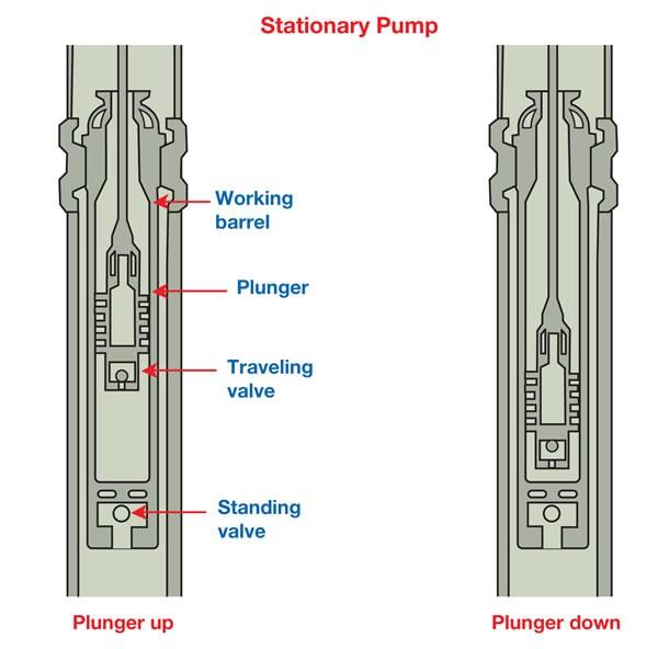
94 Figure 8

95 Figure 9 Another less common type of rod pump is the three-tube pump. This pump uses an inner plunger and an outside barrel that telescope down in a concentric manner around a standing barrel, thus forming a long fluid seal between the barrels. Because this pump does not use mechanical seals, it performs well with abrasive fluids in sandy wells. The casing pump (Figure 10) is a special type of rod pump in which a packer, placed at either the top or bottom of the working barrel, provides the fluid pack-off between the working barrel and the casing. No tubing is used. Casing pumps are generally used in large volume, shallow pumping applications.

96 Figure 10 API PUMP CLASSIFICATIONS The API classification for subsurface pumps, set out in API Specification 11AX (2001), is based on the specification of three elements of the pump: 1. Whether it is a rod-type or tubing-type pump 2. Whether it has a stationary or traveling working barrel and the type of barrel and plunger installed 3. Whether it has a top or bottom seating assembly (for rod pumps with stationary barrels), or anchor (an anchor is a mechanism that keeps one section of the pump stationary so that the pump can operate properly. It is also referred to as a hold-down ).

97 The API classification uses a three-letter code. Each letter refers to one of the three elements above. The full range of API pump classifications is shown in ( Figure 11) (API pump classifications. After API Spec. 11AX) : Figure 11 Pumps (a) and (b) in this figure are examples of stationary barrel, top hold-down pumps. Top hold-down pumps are recommended for use in sandy wells, because sand particles cannot settle over the seating nipple. This makes the pump easier to remove. These pumps are also good for wells with low fluid levels, because the standing valve is submerged deeper than it would be with a bottom hold-down pump. Pump (a) has the API classification RHA. o R means that it is a rod-type pump,

98 o o H signifies that it has a stationary, heavy-wall barrel, and A is used to indicate a top anchor. The top anchor refers to the fact that the standing valve is held in place from above. If the stationary, heavy-wall barrel is changed to a stationary, liner barrel, the designation for the pump changes to RLA. In this case, only the middle letter changes in our pump classification. Pump (b) is similar to the type of RHA pump. Again, it is a rod-type pump, but it has a stationary, thin-wall barrel and a top anchor. Its designation is RWA. If a soft-packed plunger is installed, then the designation changes to RSA. A rod-type pump with a stationary, heavy-wall barrel and a bottom anchor is an RHB pump (pump (c) in the figure). Note that for a bottom anchor pump, the standing valve is held from below and a (B) designation, rather than an (A) designation is used. If the barrel is changed to a stationary liner barrel, the designation changes to RLB. An RWB pump (pump (d)) has the same configuration, but with stationary, thin-wall barrel. If a soft-pack plunger is used in the pump, the designation is RSB./li> A traveling, heavy-wall barrel with a bottom anchor on a rod pump (pump (e)), is designated RHT. If the traveling barrel is a liner barrel, the designation is RLT. Pump (f) is the same type of pump, but with a thin-wall traveling barrel; its designation is RWT. If a soft plunger is added, the designation is RST. If, instead of a rod-type pump, a tubing pump with a heavy-wall barrel is used, then the designation is TH (pump (g) ). (If a liner barrel replaces the heavy-wall barrel, the designation is TL. A tubing pump with a heavy-wall barrel and a soft-pack plunger is given the designation TP (pump (h) in Figure 12). Note that a metal plunger is used in situations where a specific designation is not given. NOTE: There is no particular need to try and memorize each of the sixteen designations just covered. It is sufficient to know that the API classification exists and how to use it. It should be noted that, only three or four of these designations are generally used. Standard Designations for a Complete Pump Building on the general classifications above, the API has developed standard designations for a complete pump (API Specification 11AX, 2001). The designation consists of a 12 character, alphanumeric code (XX-XXX-X-X-X-X-X-X-X) as shown in Table 1(after API 11AR, 2000): TABLE 1: API Designation for Subsurface Pumps (after API 11AR, 2000) Characters 1,2 3, 4, 5 XX Designation/Description Tubing size: inch O.D inch O.D inch O.D inch O.D. XXX Pump bore (basic):

99 TABLE 1: API Designation for Subsurface Pumps (after API 11AR, 2000) Characters 1,2 3, 4, Designation/Description inch inch inch inch inch inch inch inch inch X Type pump: R - Rod T - Tubing X Type of barrel: (For metal plunger pumps) H - Heavy wall L - Liner barrel W - Thin wall (For soft-packed plunger pumps) S - Thin wall P - Heavy wall X Location of seating assembly: A - Top B - Bottom T - Bottom, traveling barrel X Type of seating assembly: C - Cup type M - Mechanical type X Barrel length, feet X Nominal plunger length, feet X Total length of extensions, whole feet

100 To illustrate the use of the API designation, we may use the information from Table 1 to describe an API pump designation for a rod-type, stationary pump with a heavy-wall barrel, a metal plunger, and a top anchor using a mechanical-type seating assembly, to be set in inch tubing, with a pump-bore size of 1.5 inches. The plunger-length is 4 feet and there are no extensions to be added. The first two characters refer to a tubing size code. The 1.9-inch O.D. tubing, for example, is code number 15; a 3 1/2-inch O.D. tubing is code number 30. In this example, with 2-3/8inch O.D. tubing installed in the pump, so the code number 20 are the first characters of the pump designation. The next three characters refer to the code for the pump bore size. There are nine pump bore sizes and each has its own three-number code referring to sizes ranging from 1 1/16 inches through 2 3/4 inches in diameter. In this example, a bore size of 1 1/2 inches, the next three characters will be the number 150. The next four characters refer to a description of the pump. o o o o The first character specifies whether the pump is a rod or tubing pump. The example pump is a rod type pump, designated by the letter R. The second character refers to the type of barrel and specifies whether it is a heavy-wall, a thin-wall or a liner barrel. The example pump has a stationary, heavy-wall barrel, designated by the letter H. The third character refers to the location of the seating assembly, whether top or bottom, and if on the bottom, whether it is a stationary or traveling barrel. The example pump has a top anchor, and this is designated by using the letter A. The fourth character in this series refers to the type of seating assembly. There are only two choices: a cup-type assembly, indicated by the letter C, or a mechanical seating assembly, indicated by an M. The example pump has a mechanical assembly so the letter M is placed in the fourth position. A rod-type pump with a stationary, heavy-wall barrel, a metal plunger, and a top anchor with a mechanical-type seating assembly will have the designation RHAM. The next three characters refer to pump length. The first character refers to the barrel length in feet. For this example, it is 8 ft. The second character refers to the nominal plunger length, again in feet. A rule of thumb states that to limit fluid slippage, pump plungers should be: o o o 3 feet long in wells less than 3,000 feet deep 3 feet plus 1 foot in length for each 1,000 feet between 3,000 and 6,000 feet of depth 6 feet long for wells 6,000 feet and deeper One exception to this rule is that shorter plungers should be used for pumping viscous oils. For thisexample, assume a plunger length of 3 feet. The final character is the total length of extensions to the barrel, again expressed in feet. Extensions of 6 inches to 4 feet can be added to both ends of a heavy-wall barrel. These extensions are used primarily to prevent scale buildup within the barrel. For the example pump, assume an extension length of 2 feet. Therefore, for this example, the final API pump designation would be RHAM

101 In order to purchase a pump, the only additional information needed would be the type of material that the liner or barrel and plunger are to be made of, the plunger clearance, the valve material, and the length of each extension to be installed. SUBSURFACE PUMP SELECTION Selecting a subsurface pump for a beam pumping system is a matter of estimating the pump displacement that corresponds to a desired production rate, and then determining the optimal combination of stroke length, pump speed and plunger diameter for this displacement. Once the pump is sized, we can consider what type of pump is most appropriate for the given set of operating conditions. PUMP DISPLACEMENT REQUIREMENTS A subsurface pump displaces a volume defined by its stroke length, pump speed (strokes per minute), plunger diameter and volumetric pump efficiency: PD = S p N D 2 E p (1) where PD = pump displacement at 100 percent volumetric efficiency, B/D S p = effective plunger stroke length, inches N = pumping speed, strokes/min D = plunger diameter, inches Ep = volumetric pump efficiency. This quantity is usually less than 1.0 for the following reasons: Leakage of fluid around the plunger The volume of fluid that slips down around the plunger during a pump stroke, and thus is not actually displaced, is known as slippage. Foaming of the fluid within the pump When this occurs, the pump becomes less efficient because it not only displaces fluid but also compresses the gas phase of the foam. Shrinkage of the fluid The fluid pressure and temperature decrease it is produced to the surface. This causes gas to come out of solution and the volume of the produced liquid to shrink by a factor corresponding to the formation volume factor at the pump depth. Local operating conditions determine the pump efficiency, which is typically in the range of 70 to 80 percent. STROKE EFFICIENCY (ES) The effective stroke length (Sp) in Equation 1 is the stroke length at the pump. Because of rod stretch and contraction, acceleration and inertial effects, Sp will be considerably shorter than the polished rod stroke length measured at the surface. For our initial pump sizing determination, we may define the stroke efficiency (E s): (2) This quantity is typically on the order of 0.75 to A more precise determination of Sp is performed as part of the detailed rod pump system design. ACTUAL PUMP REQUIREMENTS Taking into account the stroke efficiency, we can modify Equation 1 to determine the pump requirements for a desired surface production rate:

102 (3) where q D S N Ep Es = = = = = = surface production rate, B/D pump diameter, inches stroke length at surface, inches pump speed, stroke/minute pump efficiency, fraction stroke efficiency, fraction Example: The pumping unit currently in place at a well has a stroke length of 86 inches. What minimum plunger diameter is required to attain a production rate of 300 STB/D at a pump speed of 14 strokes per minute, assuming pump and stroke efficiencies of 80 percent? Solution: For the conditions of this example, a 2-inch plunger would be more than adequate for a 300 STB/D rate. But many other combinations of S, N and D could be used to attain this rate. The challenge in sizing a subsurface pump is to determine which of these combinations is optimal. PUMP SIZING Pump sizing entails placing certain limits on plunger diameter, stroke length and pump speed. For example, if the plunger diameter is too large, it may impose unnecessarily high stresses on the sucker rods and surface equipment. If it is too small, it will require high pump speeds to achieve the necessary production rate, resulting in higher peak loads on the equipment. Therefore, for a desired production rate, we must find an optimal combination of plunger diameter, stroke length and pump speed. PLUNGER SIZE We begin the selection procedure by determining the optimal pump plunger size for a desired surface production rate. This is done in Table 1 for well depths of up to 8000 feet, assuming a pump efficiency of 80 percent (the table values are based on an internal report of the Bethlehem Steel Company). In this case, for example, a plunger diameter of 1.25 inches would be recommended for a surface production rate of 100 barrels per day at a pump depth of 5000 ft. Table 1: Optimal Pump Plunger Diameters (inches) (After Bethlehem Steel Co. Sucker Rod Handbook (1958) and Brown (1980)) Surface Production, B/D at Ep = 80% (for polished rod stroke lengths of 74 inches or less) Net Lift, ft

103 Having established an optimal range of plunger diameters, we can consult the pump manufacturer to select the appropriate pump type and production tubing diameter. Table 2 shows a typical manufacturer s recommendation. Table 2: Recommended Tubing Diameters for Various Pump Bores (After Axelson, Inc., 1980) Pump Type RH (Rod, Heavy Wall) RW (Rod, Thin Wall) TH (Tubing, Heavy Wall) Tubing size, inches Pump bore, inches to STROKE LENGTH AND PUMP SPEED The optimal stroke length-pump speed (SN) combination is based on establishing a maximum practical limit below which the rods have sufficient time to free-fall through the fluid on the downstroke. (Figure 1) illustrates this limit graphically for the example of a conventional pumping unit (such data are available from the manufacturer for various pumping unit types).

104 Figure 1 In this figure, the stroke length, in inches, is plotted on the vertical scale, and the maximum practical limit of stroke length and pump speed is indicated by the blue line. During the downstroke, the rods should be allowed to free-fall to avoid excessive stress on the polished rod clamp and hanger bar. Therefore, we must select a stroke length and pump speed that fall below this limit. Assume, for example, the following conditions: Desired surface production rate = 400 STB/D, Pump efficiency = 80 percent Plunger diameter = 2 inches.

105 Stroke efficiency = 85 percent. By rearranging Equation 2 and substituting the specific values above, we obtain a relationship for SN: = 1262 SPM This value is shown in the figure. Any combination of stroke length and pump speed that falls along or to the left of this line will satisfy this specific pump design. The point where this line intersects the maximum practical limit line suggested by the manufacturers is at a stroke length of about 45 inches and a pump speed of about 28 strokes/min. (This pump speed is higher than would generally be seen in the field). As a first approximation in designing the balance of the rod pump system, use a pump design specification of D = 2 inches, S = 45 inches and N = 28 SPM. Note that the above design procedure is not absolute. A number of wells have operated very efficiently at pump speeds above the designated maximum. Local experience will provide the practical knowledge needed to modify design parameters. ROD STRING DESIGN The API has established standard specifications for the fabrication of sucker rods, including pony rods, polished rods, couplings, and sub-couplings (API Spec 11B, 1998). This publication shows that sucker rods are usually made in 25 ft lengths, except in California where they come in 30 ft lengths. The six standard rod diameters are 1/2, 5/8, 3/4, 7/8, 1, and 1 1/8 inch. MATERIALS Steel sucker rods normally have an iron composition of greater than 90 percent. Other elements are added to the steel alloys to increase hardness, reduce oxidation, and combat corrosion. For example (Weatherford, 2005): API Grade C rods are designed for light-to-medium load applications in non-corrosive wells; they have minimum and maximum tensile strengths of 90,000 and 115,000 psi, respectively. API Grade D rods are designed for heavy loads in non-corrosive or inhibited environments, and have tensile strength limits of 115,000 and 140,000 psi. API Grade K rods are fabricated from AISI 4623 nickel-molybdenum-alloy steel, and are designed for light-to-medium load applications in corrosive wells. API Grade KD63 rods are fabricated from AISI 4720 nickel-chromium-molybdenum-alloy steel, and are designed for heavy load applications in effectively corrosive wells. One standard operating practice is to run grade D rods except where severe corrosion or H 2S embrittlement may be a problem. Higher tensile strength rods are available for special applications (e.g., Weatherford S-88 and EL, Norris 97, etc.). Such rods must be handled with care because they may lose their high strength properties if damaged. Fiberglass sucker rods were introduced in the early 1970 s. Initially, their main area of application was in corrosive wells, but it later became clear that fiberglass rods offer additional benefits. Their lighter weight (about 70% less than steel rods) reduces the load on the pumping unit system, allowing for higher production without changing the pumping unit. In addition, when combined in the proper proportions with steel rods, fiberglass rods can produce longer pump strokes than stiffer, all-steel rod strings. At the same time, fiberglass rods are more expensive than

106 steel rods. They also increase the complexity of the installation design, and they require a greater degree of care in the field (Gibbs, 1991). ROD STRESS CALCULATIONS It is important to not exceed the maximum allowable rod stress. To calculate the maximum rod stress, we may use the Modified Goodman equation (or, as seen in many publications, the Modified Goodman diagram): (1) S A= (0.25 T Smin) x SF where: SA = maximum allowable rod stress, psi T = minimum tensile strength, psi Smin = minimum rod stress, psi SF = service factor The specifications for tensile strength, T, have been calculated for each API rod grade. The minimum rod stress, Smin, is measured directly or estimated for the proposed application; it is equal to the minimum polished rod load divided by the cross-sectional area of the rod. The service factor, SF, depends on the environment in which the rods will be placed (Table 1). SF will be 1.0 for API grade C and D rods, when used in non-corrosive environments, but less than 1.0, for saltwater and H 2S environments. Note that the service factor for corrosive environments is lower for grade C rods than it is for grade D rods. Table 1: Service Factors for Sucker Rods (after Brown, 1980) Service API Grade C Rods API Grade D Rods Non-corrosive Salt water Hydrogen sulfide Example: Use the Modified Goodman equation to calculate the maximum rod stress for a grade C rod operating in a saltwater environment; Smin =10,000 psi the minimum tensile strength, T, = 90,000 psi the service factor, SF, in saltwater for grade C rods is Substituting these values into Equation 3 yields: S A = (0.25 x 90, x 10,000)(0.65) = 18,281 psi. This calculated maximum rod stress should not be exceeded during pumping operations. In general, maximum allowable rod stresses under working conditions should not be higher than 30,000 to 40,000 psi. High tensile-strength rods are rated at 40,000 to 50,000 psi for use in noncorrosive environments. TAPERED ROD STRINGS The most common design for a rod string longer than about 3,500 feet is a tapered design, using combinations of rods with different diameters, and installed with the largest diameter rod at the top and the smallest diameter rod at the bottom. API design procedures for tapered strings are based on a maximum of four different rod diameters, although commercially available software packages for rod system design can accommodate more sizes.

107 One fundamental design criterion used for a tapered rod string is that the string should have approximately the same unit stress in the top rod of each section. That is, the rod loads in the top rod of each section divided by their respective cross-sectional areas should be equal. This provides a safe design even if some corrosion pitting occurs. In order to select the appropriate tapered rod string for a specific well, refer to API Recommended Practice 11L (1988; reaffirmed January 2000). Data from one of these tables is reproduced in Table 2. The sample information given is for a 5/8 1/2 tapered rod string. Table 2: Rod and Pump Data for 5/8-inch - 1/2 inch Tapered Rod String (After API RP 11L) Rod No. Plunger Diameter (D) inches Rod Weight (Wr), lb. per foot Elastic Constant (Er), 106 in/lb-ft Frequency factor (Fe) Rod string, % of each size /8 inch 1/2 inch The first column in Table 2 is the API rod number designation, given in a shorthand form where 5 indicates 5/8 inch, and 4 indicates 4/8, or 1/2 inch. The second column is the pump plunger diameter. The third, fourth and fifth columns refer to certain rod constants, while the final two columns show the recommended percentages of each diameter rod to be used in a tapered rod string for this specific rod number designation. For example, for a plunger diameter of 1.06 inches, the right-hand columns show that 44.6% of the string should consist of 5/8-inch rods and 55.4% of 1/2-inch rods. For a 5000-foot well, this would correspond to: x 5000 = 2,230 ft of 5/8-inch rods on top, and x 5000 = 2770 ft of 1/2-inch rods on bottom. Because rods generally come in 25 ft lengths, these two numbers would be adjusted to 2,225 and 2,775 ft, respectively. Using the data for a 3/4-5/8-inch ( 75 ) tapered string as given in Table 3, a 1.06-inch plunger would require 27% of the rod string to have 7/8-inch rods, 27.4% to have 3/4-inch rods, and 45.6% to have 5/8-inch rods. For the same 5000-foot well as considered above, this would yield a design made up of 0.27 x 5000 = 1350 feet of 7/8-inch rods at the top, x 5000 =1375 feet of 3/4-inch rods in the middle section, and finally, x 5000 = 2275 feet of 5/8-inch rods on the bottom.

108 Table 3: Rod and Pump Data for 3/4-inch - 5/8 inch Tapered Rod String (After API RP 11L) Rod No. Plunger Diameter (D) inches Rod Weight (Wr), lb. per foot Elastic Constant (Er), 106 in/lb-ft Frequency factor (Fe) Rod string, % of each size 7/8 inch 3/4 inch 5/8 inch Designing a pumping system using the API procedure is an iterative process, including the design of sucker rod strings. First, select a tapered rod string and calculate whether the maximum rod stress exceeds the maximum limits for the class of rods used. If it does, then it is necessary to select other rod number designations until a string is found that will satisfy the design limitation. Using the API design calculations, one of these tapered strings might meet the design limitations. If not, a heavier or lighter rod string should be designed. ROD LOADS DURING PUMPING Once the basic properties of the sucker rods and the design parameters of the rod string are established, the next step in designing the string is to calculate the rod loads during pumping operations. This information is used to size the pumping unit. Consider the reciprocating motion of the polished rod and the actions of the traveling and standing valves during the pumping cycle. Throughout this cycle, the load on the sucker rod string varies continuously. The maximum load occurs shortly after the beginning of the upstroke, when the traveling valve closes. The polished rod must carry the full weight of the fluids, the rods, and the added inertial effects that occur as the motion of the rods is reversed. This is known as the Peak Polished Rod Load, or PPRL. The minimum load occurs shortly after the beginning of the downstroke, as the traveling valve opens. At that point, the rods no longer carry the fluid load and the inertial effects are reversed, thereby reducing the total rod load below the weight of the rods in the produced fluids. This is known as the Minimum Polished Rod Load, or MPRL. To calculate the maximum and minimum rod loads, we begin with the PPRL. This is equal to PPRL = W - Br + Fo + I Where W = weight of rods in air, lb Br = buoyancy of rods in fluids, lb Fo = weight of fluid column, lb I = effects of inertial and acceleration forces, lb. Consider, for example, the following tapered sucker rod string: 1350 ft of 7/8-inchrods (2)

109 1375 ft of 3/4-inch rods 2275 ft of 5/8-inch rods The average density of the hole fluid is 55 lb/cu ft ( = 0.88). The average unit weight of the rods in air is given as lb/ft. Thus, the total weight of the rods in air is simply equal to: W = (5000 x 1.566) = 7830 lb The second term, the buoyancy of rods in the produced fluids, is equal to the weight of the fluids that the rods displace. It is calculated as follows: (3) Br = W or where = specific gravity of the produced fluid, dimensionless W = weight of rods in air, lb 62.4 = density of water, lb/cu ft 488 = density of steel, lb/cu ft. Using Equation 3, Br = W = (0.128)(0.88)(7830) = 882 lb. The weight of the rods in fluid, Wrf, is equal to the weight of the rods in air minus the buoyancy effect of the rods, or: Wrf = W - Br = = 6948 lb. The weight of the fluid column supported by the net plunger area, Fo, is equal to the density of the produced fluid multiplied by the net plunger area, multiplied by the height of the static fluid level. The net plunger area is equal to the cross-sectional area of the plunger minus the area of the rods. The suggested API procedure, however, disregards the area of the rods in these calculations. Fo = x A x H (4a) where = density of fluid, lb/cu ft A = area of plunger, sq ft H = fluid level, ft Substituting = 62.4, and A = D2/(4 x 144), where D is the plunger diameter in inches: F0 = 0.34 D2H (4b) Where is 0.88, the plunger diameter is 1.06 inches and the static fluid column height is assumed equal to the pump depth of 5000 ft: Fo = (0.34)(0.88)(l.062)(5,000) = 1681 lb. This is the weight of the fluid column. Returning to Equation 2 and substituting the calculated values yields a PPRL value of 8629 lb plus the effects of the inertial and acceleration forces, which are still unknown. Due to the complex behavior of the polished rod, predicting the effects of these forces is the most difficult part of the analysis. The rod string stretches and contracts in response to a cyclic motion (not a simple harmonic) and to motions of the crank and pitman that are different for each type of pumping unit. In addition, because of the elasticity of the sucker rod system, stress waves run up and down the rod in response to the various forces that affect the rod.

110 Several methods may be used to estimate the effect of inertial and acceleration forces in the polished rod loads. One method is to make simplifying assumptions about the behavior of the rod and the pump motion; however, this method is not used often today. Another method is to calculate rod loads by solving the nonlinear partial differential equations that represent the behavior of the rod string. Gibbs, originally on his own and later with Neely at Shell Oil Co., solved these equations in an effort to analyze pump operation rather than pump design (Gibbs, 1963; and Gibbs and Neely, 1966). Their work uses known values of peak polished rod loads at the surface to calculate the behavior of the pump in the subsurface. Yet another method is the API design procedure that uses empirical correlations derived from repeated observations of pump behavior. This research was conducted at the Midwest Research Institute where computer simulations of rod-pumping systems were performed. By simulating a wide range of pumping conditions, the Institute was able to develop correlations for predicting polished rod loads. Both analytical solution methods and the API procedure are incorporated into many commercially available software programs for rod pump system design. API SYSTEM DESIGN PROCEDURE Designing a rod pumping system involves complex calculations of the dynamic relationships between production rates and stresses at various points in the system. For many years, the standard for such design calculations has been the API Recommended Practice for Design Calculations for Sucker Rod Pumping Systems (RP 11L). First published in 1966, updated in 1988 and reaffirmed in January 2000, this recommended practice involves the use of dimensionless variable correlations for optimizing design parameters. Although API-RP 11L has been supplemented and in some cases supplanted by PC-based programs that are quicker to use and more general in their application, it is discussed here to provide some insight into the considerations involved in rod pump system design. ASSUMPTIONS AND LIMITATIONS The following assumptions are incorporated into API RP 11L: Applies to conventional pumping unit motion. Pumping unit employs medium-slip prime mover. Steel rod string in the case of tapered strings, the rods become smaller with depth. Negligible friction at the stuffing box and in the pump. Pump completely liquid-filled (no gas interference or fluid pound). Anchored tubing (a correction formula is included to approximate effects of unanchored tubing). Pumping unit in balance. DIMENSIONLESS VARIABLES The experimental work conducted at the Midwest Research Institute (Kansas City, Missouri, 1964) on sucker rod pumping, later adopted by the API, consisted of numerous analog computer simulations over a wide range of pump operating conditions. The results are correlated based on two dimensionless variables: dimensionless pump speed and dimensionless rod stretch. The dimensionless pump speed variable may have two forms: N/No or N/N o.

111 N/No, is the pump speed in strokes per minute (N ), divided by the natural frequency of the string (No ). N/N'o is equal to (N/No )/ Fc, where Fc is the frequency factor of the rod string. Fc is equal to 1.0 for non-tapered rod strings, and is greater than 1.0 for tapered rod strings. Table 4.1 of API RP 11L lists Fc values for various tapered rod strings. If a rod string is non-tapered, then N/No = N/N'o. These dimensionless variables are calculated as follows: Where A = speed of sound in steel rods (approximately 980,000 ft/min) L = rod length, ft Substituting this value of No into the dimensionless variable, (1) and (2) Thus, for a given or assumed pump speed, rod string length and frequency factor, we may calculate a value for each of these dimensionless variables. Before making this calculation, consider the second dimensionless variable, the dimensionless rod stretch, defined as Fo/Skr. where Fo = the static fluid load in pounds S = the polished rod stroke length, in inches k r = the spring constant of the rod string. k r can be derived from Er (the reciprocal of kr multiplied by the rod length, L), which is also listed in Table 4.1 of API RP 11L (Figure 1: Excerpt from Table 4.1 of API RP 11L). Skr represents the load in pounds required to stretch the rod string the length of the polished rod.

112 Figure 1 The dimensionless rod stretch term represents the rod stretch caused by the static fluid load; it is given as a fraction of the polished rod stroke length. (Fo/Skr = rod stretch as a fraction of polished rod stroke length for example, if Fo/Skr = 1, then the rod string will stretch an amount equal to the length of the polished rod. The value of this dimensionless variable may be easily calculated for a known or assumed polished rod stroke length. On a practical note, observations have determined that under-travel and over-travel of the pump plunger can be prevented if N/No' is less than 0.35, and Fo/Skr is less than From the work performed at the Midwest Research Institute, five correlations were developed these are shown in API RP 11L as Figures 4.1, 4.2, 4.3, 4.4 and 4.5. These five correlations, based on the two dimensionless variables for their presentation, are used to systematically develop the API design procedure for a pumping system. The first three correlations affect the rod and downhole pump system specifically, the plunger stroke length, the peak polished rod load, and the minimum polished rod load. The last two correlations are used to calculate peak torque and polished rod horsepower. DESIGN EXAMPLE: To demonstrate the use of these correlations consider a well that is to be pumped at a rate of 100 B/D. The well conditions are: Fluid level (H) and pump depth (L) = 5000 ft Tubing diameter = 1.9 inches. Tubing is anchored A tapered sucker rod string (API 75), consisting of 1350 ft of 7/8-inch rods, 1375 ft of 3/4-inch rods, and 2275 ft of 5/8-inch rods, is calculated to be sufficient for this design. These grade D rods have a maximum allowable rod stress of psi. Plunger diameter = 1.06 in. For preliminary design, pump speed (N) = 16 strokes/min Polished rod stroke length (S) = 64 inches.

113 Specific gravity ( ) of the pumped fluid = Substituting these data into the equation for pump displacement, using the polished rod stroke length, S, as an estimate of the pump stroke length, and assuming a pump efficiency of 100 percent, we obtain: PD = Sp N D 2 Ep = (0.1166)(64)(16)(1.06) 2 =135 B/D (3) This quick calculation gives us a pump displacement of about 135 B/D, which should satisfy the well s IPR-calculated objective of 100 B/D. PLUNGER STROKE CORRELATION The first correlation allows us to calculate the plunger stroke length ( Figure 2: Plunger stroke correlation, after API RP 11L).

114 Figure 2 The dimensionless pump speed, N/No, is shown on the horizontal axis. The bottomhole plunger stroke length divided by the polished rod stroke length (S p/s ) is plotted on the vertical axis. This ratio reflects the effect of rod stretch on the effective plunger stroke length. The plot shows a series of curves, each for a different value of the dimensionless rod stretch (Fo /Skr). Because the values of N/No and Fo /Skr are known or can be calculated from the given data we may use this correlation to calculate a value for Sp /S. For the example problem, N/No is calculated as follows: N/No = NL / 245,000 = (16 * 5,000) / 245,000 = 0.326

115 For the selected tapered rod string, F c is equal to 1.191, and so: N/ N'o = N / (No Fc ) = / N/ N'o = The dimensionless rod stretch is equal to Fo/Skr. Fo, the weight of the fluid supported by the rods, is F0 = 0.34 D2H (4) where = specific gravity of fluid of fluid, lb/cu ft = D = plunger diameter, inches H = fluid level, ft Where is 0.88, the plunger diameter is 1.06 inches and the static fluid column height is assumed equal to the pump depth of 5000 ft: Fo = (0.34)(0.88)(l.062)(5,000) = 1681 lb. The polished rod stroke length (S) is 64 inches, and the reciprocal of k r is equal to the elastic constant, E r for the example rod string multiplied by its length, L (i.e., 1/k r = E rl). From API manual RP 11L, we obtain, E r. E r = x 10-6 in/lb ft and substitute the value into the relationship for the dimensionless term: Fo/Skr = (1.681 * * 10-6 * 5000) / 64 Fo/Skr = 0.13 Note that N/N'o < 0.35, and Fo / Skr < This puts them within the practical limits for preventing under-travel and over-travel of the pump plunger mentioned above. Referring back to (Figure 2), we see that with known values for the two dimensionless variables, we arrive at a value of S p / S = This means that if the tubing is anchored, as in this example, the bottomhole plunger stroke length is equal to 98 percent of the polished rod stroke length at the surface. Specifically, for a polished rod stroke length of 64 inches, the bottomhole stroke length will be 62.7 inches. If the tubing is not anchored, the plunger stroke length corrected to account for the tubing contraction during the upstroke. This term is found by the following formula: Tubing contraction = Et Fo L (5) Where Et = coefficient of elasticity for the tubing, in/lb ft Fo = weight of fluid on rods, 1b L = tubing length, ft. For 1.9-inch tubing, Et has a value of 0.5 x 10-6 in/lb ft. With Fo equal to 1681 lb, and L equal to 5000 ft, the tubing contraction in unanchored tubing, is: Tubing Contraction = (0.5 x 10-6)(1681)(5000) = 4.2 in. So, in this example, the net plunger stroke length would be ( ) = 58.5 inches. We can now calculate the subsurface displacement. Assuming that the tubing is anchored, the pump displacement is: PD = SpND 2 = (0.1166)(62.7)(16)(1.06) 2= 131 B/D. This more than meets the example expected inflow rate of 100 B/D. In fact, it allows more downtime per day for maintenance. However, had the pump displacement rate not met the production objective, it would be necessary to revise the assumed pump data and repeat the calculations. Note that to determine the production rate at the surface, we must incorporate the pump efficiency (Ep) into the calculation.

116 PEAK POLISHED ROD LOAD CORRELATION The second API correlation can be used to calculate the peak polished rod load ( Figure 3: PPRL correlation, after API RP 11L). The same dimensionless variables, whose values are known, are plotted in the same general locations. In this case, the horizontal axis is simply N/N o. It is the vertical axis that is changed, and is now equal to Fl/Sk r. The terms in the denominator are already defined; their values were calculated earlier. Fl, the only unknown, is referred to as the peak polished rod load factor. Figure 3 The dimensionless pumping speed, N/No, is equal to The dimensionless rod stretch, Fo/Skr, is equal to With these two known values, we can use ( Figure 3) to find a value of 0.37 for Fl/Skr.

117 Because Skr is known, it is possible to calculate Fl. Note that Fl must be added to the weight of rods in the produced fluids to give a value for the peak polished rod load in pounds. It thus represents two terms: the weight of the fluid carried by the rods and the load caused by the inertial-acceleration forces. The peak polished load, then, is equal to: PPRL = Wrf + Fl (6a) Where PPRL = peak polished load, lb W rf = weight of the rods in fluid, lb F1 = weight of fluids on rods plus inertial-acceleration forces, lb Or, in terms of the correlation: (6b) Where PPRL = peak polished load, lb Wrf = weight of the rods in fluid, lb F1 = weight of fluids on rods plus inertial-acceleration forces, lb Skr = the load in pounds required to stretch the rod string the length of the polished rod. For this sample problem, we determine the weight of the API 75 rod string in the produced fluid to be 6948 lb. The second term (F l/skr) is equal to All that is needed to calculate PPRL is the value of Skr. The spring constant for the rod string (k r) is equal to the reciprocal of the coefficient of elasticity of the rod string (E r ) multiplied by the length of rods (L): 1/k r = (E r)(l) 1/kr = (0.997 x 10-6 )(5000). Then, taking the reciprocal, we obtain: kr = With a polished rod stroke length, S, of 64 inches, Sk r is calculated : Skr = (64)(200.6) = lb. With this information the peak polished rod load for the example can be calculated: PPRL = W rf + ((F l/skr) * Skr) PPRL = (0.37 * 12838) = lb. This value represents the best estimate of the rod load, and can be used for design purposes. Under actual operating conditions, it may be different, but not significantly so. MINIMUM POLISHED ROD LOAD CORRELATION The third API correlation (Figure 4: MPRL correlation. After API RP 11L) involves calculating the minimum polished rod load (MPRL). This load occurs just at the beginning of the downstroke, when there is maximum downward inertial force, and the rods no longer carry the fluid load.

118 Figure 4 The two dimensionless variables are in the same relative locations, but now the term F2/Skr is on the vertical axis. F2 is defined as the minimum polished rod load factor. Using the information already obtained, with an N/No of 0.326, and an Fo/ Skr value of 0.13, the point of intersection on the vertical axis is at With the value for Skr known, we can calculate F2. F2 is the weight that must be subtracted from the weight of the rods in the produced fluid to give the MPRL. As such, it represents the inertial and acceleration force at the point of minimum load. Its calculation proceeds directly parallel to that for the peak polished rod load: (7a) MPRL = W rf -F2 MPRL = W rf - (F2/Skr * Skr ) (7b)

119 MPRL = (0.21 * 12,838) MPRL = 4252 lb. This MPRL of 4252 lb. is used for design purposes; the actual value of F2 after installation may be different. SELECTION OF COUNTERWEIGHTS Counterweights are added to a pumping unit to provide a counterbalance effect at the polished rod. We can appreciate their importance by considering what would happen if this counterbalance was not present. On the upstroke, the prime mover would have to do an enormous amount of work. An excessive torque would be exerted on the gear reducer, requiring a larger prime mover and a more substantial gear reducer. But on the downstroke, with the polished rod load substantially reduced and the force of gravity pulling the rods and plunger downward, the prime mover would have little work to do. In short, it would be practically impossible to design a system to efficiently handle such load variations. Counterweights serve to reduce these load variations by moving downward during the upstroke (thus helping to lift the rod string) and upward during the downstroke (thus keeping the rod string from falling too quickly). This reduces the size requirements for the prime mover and provides a more even load to the gearbox. For design purposes, we can estimate of an ideal counterbalance that establishes an approximately equal balance between (1) the upstroke and downstroke work done by the prime mover and (2) the net torque exerted on the gear reducer during each half of the pumping cycle. This balance should be the design objective, and is determined by calculating the maximum and the minimum loads on the polished rod during the pumping cycle and then calculating their mean value: Mean value = W rf Fo (8) Where Wrf = weight of rods in fluid, lb. Fo = weight of fluid imposed on rods, lb. The required counterbalance effect, CBE, should be approximately equal to the mean load. For API design purposes, however, the design value of the counterbalance effect for the conventional pumping unit is slightly larger than this amount in fact, it is 1.06 times larger than the mean load. CBE = (1.06) (Wrf Fo). (9) Substituting the data from the sample problem into this equation, we obtain the total required counterbalance effect: This CBE is required at the polished rod; it is transmitted there through the counterweights acting on the connecting pumping unit members. To determine the size of counterweights needed, a force balance around the various contributing structural members must be calculated that includes the effect of the unit s geometry and its contribution to the CBE. The pumping unit manufacturer provides this information. For a given pumping unit, pump stroke length, and desired CBE, the manufacturer will specify the types of counterweights to be used and where they should be placed on the unit. The actual CBE needed for a pumping unit is determined by field measurements of the peak and minimum polished rod loads. These measurements will dictate to what position the counterweights must be adjusted or, for an air-balanced unit, by how much the pressure in the cylinder must be changed. PEAK TORQUE CORRELATION

120 Consider the torque that is imposed on the crank by the low speed shaft of the gear reducer during the pumping motion. One important system design objective is to be sure that the peak torque does not exceed the manufacturer s limits. Remember that torque is equal to the force acting at right angles to a lever arm, multiplied by the length of the arm, and that torque tends to produce rotation at the point of connection. The torque of a pumping unit is provided by the prime mover, and is applied to the crank by the low speed shaft of the gear reducer that, in turn, causes the pump to operate ( Figure 5: Torque generated by pumping unit). This torque must be sufficient to cause the pump to operate in a continuous manner under normal operating conditions. Figure 5 The net torque at the gear reducer is equal to the torque caused by the well loads acting on the polished rod minus the torque caused by the counterweights acting along the crank. Because the magnitudes of these two terms change during the pumping cycle, the peak torque is defined as the maximum net torque that occurs during the pumping cycle. (Figure 6) shows the net torque imposed on a typical conventional beam pumping unit.

121 Figure 6 The dashed curves show the rod load and counterweight components of the torque during one full cycle, beginning with the upstroke. Notice that the rod load during the upstroke is positive and the counterweight torque is negative. The maximum and minimum values occur about midway through the upstroke. As one value decreases, the other increases. The values become equal and very close to zero at the top of the upstroke, and reach maximum and minimum points midway through the downstroke. The solid curve shows the net effect of the two components it reaches a maximum value (peak torque) midway through the up and down portions of the stroke. The gear reducer, then, must be designed to accommodate this peak net torque by an appropriate safety margin. Manufacturers specify the peak torque for each pumping unit. Note that the above representation is for a conventional unit and will be different for other types of units. The peak torque of a pumping unit is calculated by using two additional API correlations. Peak torque, PT, is given by the multiple of four terms:

122 (10) Where PT = peak torque, lb-in T = torque, lb-in Ta = torque adjustment factor, fraction Skr = load required to stretch rod string the length of the polished rod, lb. S = polished rod stroke length, in. Notice that the second and third terms in the example problem are already known. It is the first and the fourth terms that must be obtained from the two new correlations. The peak torque correlation is shown in (Figure 7) (Peak torque correlation, after API RP 11L). The first term in on the right-hand side of Equation 10 is shown on the vertical axis. The two familiar dimensionless variables (N/No and Fo/Skr) are shown in the same relative positions as they were in earlier correlations.

123 Figure 7 Starting from N/No =0.326 on the horizontal axis, and moving vertically upward to a value of Fo/Sk r = 0.13, we determine that the corresponding value of (2T/S2kr ) is Thus, for our example design, Equation 10 has the following form: PT = (0.32) (12838) (64/2) Ta = T a. A single unknown, Ta, remains to be determined. Where (W rf / Sk r ) = 0.3, then Ta = 1.0, and no further adjustments to the equation are necessary. Where (W rf / Sk r 0.3), then Ta differs from 1.0. In order to calculate its value under these conditions, turn to the fourth API correlation shown in (Figure 8) (Peak torque correlation, after API RP 11L, continued).

124 Figure 8 Here, the familiar dimensionless variables are found on the vertical and horizontal axis. In this case, the horizontal axis is N/No. Within the chart are percentage values ranging from positive values on the outer rim to negative values near the center. For specific values of the dimensionless variables, this chart is used to find the appropriate percentage. The value of this percentage is then used to calculate the torque adjustment constant, Ta, using the following equation: (11) Where Ta X W rf Sk r = torque adjustment factor, fraction = percentage correction = weight of rods in fluid, lb. = load required to stretch rod string the length of the polished rod, lb Using the specific values for the dimensionless variables that have been used previously (i.e., on the horizontal axis and 0.13 on the vertical axis) the percentage correction is found to be equal to about +2.5% (Figure 8, above). Substituting this value into the equation,: =1.06 When this value is included into the relationship for peak torque, PT: PT = (131,465)(1.06) = = 139,353 in/lb.

125 This is the expected peak torque of the example pumping unit. The shaft of the gear reducer should be designed to withstand a maximum torque of at least this value. Later, this design specification will be introduced into the pump unit designation. The gear reducer, acting through the V-belts, transmits the power and the rotating speed of the prime mover into the power and rotating speed needed by the pumping unit. Normally there are both high-speed and low-speed gears, and a careful selection of the gear reduction system is a necessary part of the manufacturer s overall design of the pumping unit. POLISHED ROD HORSEPOWER CORRELATION The API procedure for calculating the polished rod horsepower, PRHP, for the conventional unit is given by the following relationship: PRHP = (F3 /Skr) Skr SN ( ) (12) where F3 = PRHP factor, lb and, as defined above Sk r = load required to stretch rod string the length of the polished rod, lb S = stroke length at surface, inches N = pump speed, stroke/minute A value for F3 may be found by using the fifth API correlation, as shown in ( Figure 9) (PRHP correlation, after API RP 11L).

126 Figure 9 Notice this figure s similarity to the other API correlations. The two familiar dimensionless variables appear in the same relative positions, and the new variable appears on the vertical axis. This variable is the first term in the calculation for the polished rod horsepower. To find its specific value, enter the horizontal axis the previously determined N/N o value of 0.326, and move vertically upward to a F o /Sk r value of These correspond to F3 /Sk r = Substituting this value plus the known value of other terms into Equation 12 yields: PRHP = (0.223)(12,838)(64)(l6)(2.53 x 10-6) = 7.48 HP Knowing the PRHP, we can determine the nameplate horsepower (HPnp), which is the minimum horsepower required to run the unit: HPnp = (PRHP)(CLF) / (E surf ) (13)

127 where PRHP = polished rod horsepower, CLF = cyclic load factor E surf = surface efficiency of pumping unit, fraction The cyclic load factor (CLF) represents the additional reserve power needed to handle the cyclic beam-pumping load. For low peak torques and uniform torque ranges, the cyclic load factor is low when peak torques are low and torque ranges are uniform. If, on the other hand, the peak torques are high and the ranges are non-uniform, the cyclic load factor is high. The prime mover normally recommended for beam pumping units is the NEMA Design D electric motor. For this unit, the CLF is about For NEMA C electric motors and multi-cylinder engines, the CLF will be about These CLF values are valid for conventional and air balanced units, but will differ for MARK II units, as shown in Table 1. Table 1: CLF Values for Various Pumping Unit Types (Courtesy of Lufkin Industries, Lufkin, TX, USA) Unit Type Prime Mover Type CLF Value Conventional and Air Balanced NEMA D electric motors and slow speed engines NEMA C electric motors and multi-cylinder engines Mark II NEMA D electric motors and slow speed engines 1.10 NEMA C electric motors and multi-cylinder engines The third term in Equation 13 is the surface efficiency, Esurf. It is equal to the combined efficiencies of the motor and the moving parts of the pumping unit, including the wire lines, structural bearings, transmission, gears, gearbox bearing, and the V-belt. The mechanical efficiency is usually about 90%. The motor efficiency depends on the motor, its operating speed and load variation during a revolution of the crank. The motor manufacturer will provide motor efficiency information. For this example, assume that it is 70 percent. Esurf = (0.9)(0.7) = This information may be used to calculate the nameplate horsepower for the example problem. Assume that a NEMA D electric motor, with a CLF of 1.375, is installed. A number of factors, including polished rod horsepower, torque loading, system voltage, start-up problems and motor characteristics, will influence motor size. Substituting the known values into Equation 13 yields: HPnp = (7.48)(1.375) / 0.63 = 16.3 HP The nameplate horsepower for this NEMA D motor is found to be Notice that the motor nameplate horsepower is about two times the polished rod horsepower. Because motors come in discrete sizes, as shown in Table 2, a 20 horsepower unit would be ordered for this example application. Table 2: Recommended Motor Sizes for API Pumping Units (Courtesy of Lufkin Industries, Lufkin, TX, USA) Unit Size Recommended Motor Sizes,

128 HP There are a number of other ways to calculate the horsepower required for the prime mover. Some have been developed by manufacturers, others by individual oil companies. Table 3 shows examples of different nameplate horsepower calculations used by one manufacturer. Table 3: Alternative Nameplate Horsepower Calculations Conventional and Air Balanced Units Mark II Units Slow speed engines and high-slip electric motors Multi-cylinder engines and normal-slip electric motors ROD STRESS CALCULATIONS The last calculation in the design procedure is made to ensure that the rod stress is not too high. Maximum rod stress is equal to the peak polished rod load divided by the cross-sectional area of the top rod: Rod Stress = PPRL / Rod Area (14) In this design example, the rod stress exerted on the 7/8-in top rod is (11,698 / 0.601), or 19,464 psi. This value is well below the maximum allowable stress of psi that was specified for the Grade D rods. POLISHED ROD DYNAMOMETERS Rod-pumped wells must be monitored to ensure the continued efficient and economic operations of a field. After a pumping unit has been installed in the field, dynamometer tests of pumping wells are conducted to determine the system efficiency, and whether adjustments need to be made in stroke length, pump speed or other operating parameters. These tests are designed to answer such well performance questions as (Podio et. al, 2001): Is the well pumped off? What is the pump intake pressure? What is the pump fillage? What is the pump displacement?

129 Is the standing valve or traveling valve leaking? What is the effective pump plunger travel? What is the current pumping speed? What is the polished rod horsepower? Is the gearbox overloaded? Is the unit properly balanced? Is the downhole gas separator operating efficiently? A dynamometer survey measures the load forces acting on a rod string during a complete pumping cycle and records the forces on a chart or computer display. This display is often called a dynamometer card. The card records changes in the rod load versus rod displacement, or changes in the rod load versus pumping time (Figure 1: Example of surface (top) and pump (bottom) dynamometer cards. Courtesy Echometer Company, 2003). Figure 1 During a pumping cycle, forces acting on the rod string cause changes in the rod load. Measurements of these rod loads reflect the operation of the subsurface pump and the surface unit. Polished rod dynamometers record polished rod loads during the pumping cycle. Most common dynamometers make continuous plots of load measured against the movement of the polished

130 rod. Typical conventional dynamometers are either mechanical or hydraulic, but electronic dynamometers are also used. These dynamometers are briefly described below. MECHANICAL DYNAMOMETER A mechanical dynamometer measures rod loads by measuring the deflection of a steel ring placed between the carrier bar and the polished-rod clamp. A recording of this ring deflection is made on a paper dynamometer card, attached to a rotating drum driven by the vertical movement of the polished rod. The card traces polished-rod loads against rod vertical displacement. Its major disadvantage is that the pumping unit must be stopped before it can be installed on the polished rod. HYDRAULIC DYNAMOMETER A hydraulic dynamometer (Figure 2: Courtesy Echometer Company, 2003) can be installed while the pumping unit is running. This type of dynamometer uses a spacer installed on the polished rod between the carrier bar and the polished-rod clamp. As the unit is pumping, two load-sensing hydraulic pistons can be installed between the shoulder of the spacer and the carrier bar. The polished-rod load is transferred to the hydraulic pistons. Changes in polished-rod loads affect the hydraulic pressure. These changes in hydraulic pressure are recorded on a drum chart as changes in rod load versus rod displacement. Figure 2 ELECTRONIC DYNAMOMETER

131 The electronic dynamometer uses electronic transducers to measure well loads and rod displacements (Figure 3: Polished rod dynamometer transducer. Courtesy Echometer Company, 2003). Figure 3 An electronic dynamometer unit s main components include a load transducer (load cell), a position transducer and the electronics that provide interfacing, signal recording, and processing. The load cell, located between the carrier bar and the polished-rod clamp, uses a strain gauge to measure polished rod loads. The position transducer uses a potentiometer to measure polishedrod displacement. Accelerometers determine rod displacement so that polished-rod load and position can be recorded as a function of time. In this manner, an electronic dynamometer can produce surface dynamometer cards and supply the information needed to construct downhole cards. Portable electronic dynamometer systems usually include microcomputers that combine real-time data acquisition with easy data storage and retrieval operations, as well as performing on-line analysis of measurements and calculating downhole cards. DYNAMOMETER CARD INTERPRETATION (Figure 4) shows a dynamometer card shortly after it is recorded at the surface.

132 Figure 4 A number of measurements must be noted on the card. The first is C, the calibration constant in pounds per inch of card height. Each inch of height, then, refers to some calibrated load on the polished rod. This is determined in the field. D1 is the maximum deflection in inches. D2 is the minimum deflection in inches. CB is the counterbalance line, which is obtained by drawing a line through the dynamometer card at the point that represents the static load on the polished rod when the crank arm is horizontal. This means that the pumping unit is stopped and the load on the polished rod is measured with the crank arm at an angle of 90º or from the 12 o clock position. A 1 is the lower area of the card, measured in square inches that is, it is the area between the lower boundary and the zero line. A 2 is the area within the card shape, measured in square inches. Finally, L is the length of the card, in inches, measured along the horizontal axis from one end of the dynamometer shape to the other. The left-hand extreme of the card is the bottom of the stroke, and the right-hand extreme is the top of the stroke. With a dynamometer card for a given rod pump and the definitions above, we can make the diagnostic calculations listed in Table 1: Table 1: Diagnostic Calculations for Beam Pumping System

133 Peak polished rod load PPRL =D 1C Minimum polished rod load MPRL = D 2C Polished rod load range C(D 1 - D 2) Counterbalance effect Actual CBE = CD 3 Approximate CBE (C/L) ((A 1+(A 2/2)) Polished rod horsepower PRHP = C(A2/L) (SN/33000 x 12) The final term to be calculated is the peak torque that is exerted on the gear box under operating conditions. Normally this calculation is made using a term referred to as the torque factor, TF. The torque factor is equal to the torque that must be applied at the crankshaft to offset a one pound weight hanging on the horsehead. Thus, if a 25 ft-pound torque must be applied at the crankshaft to offset a one-pound weight hung on the horsehead, the torque factor is 25. The torque factor will vary with different crank angles. With a value for TF, the net torque calculation, which is a function of the crank angle, can be made by using the following equation: Net torque = TF (W-B) - M Sine q (Equation 15) where: W = well load for a given crank angle, pounds B = structural imbalance of pump unit, pounds (supplied by manufacturer) N = torque provided by the counterweights, ft-pounds TF = torque factor q = crank angle Using this equation, we can look at the dynamometer card, insert the crank angle on it for a number of different values of W and TF, and make net torque calculations using the above equation. Note that W is a function of the crank angle and is measured from the dynamometer card. The torque factor, TF, is supplied by the manufacturer for a given unit in 150 angles of the crankshaft. This net torque calculation should provide a plot similar to that shown in the dashed curve of (Figure 5), showing the peak torque at the maximum point on the curve. It suggests that the counterweights should be adjusted in order to even out the net torque curve. After an adjustment of the counterweights, for example, a second curve is obtained (solid curve), showing that the unit is now more balanced.

134 Figure 5 The downhole condition of the pump and its pumping action can be analyzed with a dynagraph. With the dynamometer, those terms that affect the surface operating condition can be calculated and necessary adjustments to the unit can be made. If the operation of the subsurface pump and the surface unit are satisfactory, is it possible to improve production by changing the pump stroke length, its speed or its surface control system? Generally, a unit that runs intermittently is controlled either by a timer or with a pump-off controller. Careful adjustments in the field are required to maximize production, without damaging the pumping unit. The information from dynamometer tests taken both before and after changes are made in the pumping equipment will help determine whether the adjustments have improved the operating conditions. ROD LOAD VERSUS DISPLACEMENT To understand the diagnostic procedures involved in monitoring a beam pumping system, we must first understand the principles of dynamometry. Gibbs and Neely (1966) discuss polished-rod load versus displacement for anchored and unanchored tubing. Typical plots for the unanchored and anchored tubing case are shown in the next series of figures. These plots are developed systematically. UNANCHORED TUBING

135 (Figure 1) represents the rod load as a function of displacement for unanchored tubing. Note that the load scale goes as high as 10,000 pounds, and that the pump displacement (in feet) has a coordinate system that runs from a point above the top of the subsurface pump down to the standing valve. When the plunger is at its lowest point, it carries no load; its displacement is 9 feet from the coordinate to the ground coordinate system, but it is stationary with respect to the stretching tubing. Figure 1 In (Figure 2), as the traveling valve reaches point C, the entire fluid load is supported by the rods, until it begins to transfer to the tubing at point D.

136 Figure 2 In (Figure 3), as the traveling valve reaches point E, the transfer of the load from the rods to the tubing is almost complete, but the tubing continues to stretch somewhat. At point F, the entire fluid load is now supported by the tubing, causing the tubing to stretch to its greatest length. The plunger now descends with respect to both the ground and tubing coordinate systems. At this point, there is no load on the traveling valve and it continues to descend until it reaches a displacement position, indicated by point A. The cycle then repeats.

137 Figure 3 ANCHORED TUBING If the tubing is anchored, it will not stretch or contract in response to the movement of the pump, and the ideal load-displacement diagram will have the appearance shown in ( Figure 4) (Ideal load-displacement diagram for a pump with anchored tubing).

138 Figure 4 PUMP VALVE DYNAMOMETERS Efficient operation of a sucker-rod pump depends on the integrity of the standing and traveling valves. If these valves lose their ability to hold a seal, the lifting capacity of the pump is affected. Therefore, the valves should be tested periodically with a dynamometer. TESTING THE STANDING VALVE Dynamometer testing of the standing valve requires that pumping unit to be stopped near the bottom of the downstroke. The initial polished-rod load is recorded on the dynamometer chart. Since the fluid load is completely carried by the standing valve, the polished-rod load recorded at the start of the test will measure only the buoyant weight of the rod string. When the standing valve holds a good seal, the polished-rod load will remain steady, resulting in a line on the dynamometer card that falls on the first measurement. If there is a leak in the valve seat, the pressure immediately below the traveling valve will decrease, then slowly close. As the test proceeds, the fluid load initially carried by the standing valve will move to the traveling valve.

139 This movement increases the load of the polished rod, and will be recorded on the dynamometer chart. The rate of load increase is directly proportional to the severity of the leak in the standing valve and it is not uncommon for a leaking standing valve to show a load increase in about 20 seconds. This test should be repeated. If the same results are obtained, then the test indicates that the seat of the standing valve is cut. If the valve holds during some of the tests, then a damaged valve ball is indicated. TESTING THE TRAVELING VALVE Testing the traveling valve will help to distinguish whether the traveling valve or the barrel-plunger fit is leaking. To start the test, the pumping unit is stopped near the top of the upstroke and the initial polished-rod load on the dynamometer is recorded. The initial recorded polished-rod load measures the buoyant weight of the rod string and the fluid load acting on the plunger. The standing valve is open so it carries no load. If the seal in the traveling valve is good, and additionally, the pump barrel and plunger fit is good, then no change in polished-rod load should be observed over the test period. A leak either in the traveling valve or between the pump barrel and plunger will allow fluid to pass through the traveling valve. This leak will slowly force the standing valve to close. Once closed, the fluid load transfers to the standing valve and the tubing, and this load transfer will be observed on the dynamometer card. The initial polished-rod load (rod-string weight plus fluid load) recorded on the card will be greater than the loads measured later in the test. The rate of load decrease is proportional to the leak rate. This test cannot distinguish between a leaking traveling valve and leaking caused by a worn barrel or plunger. This test should be repeated at different points in the upstroke. Load differences observed at different depths can help to identify the location of the leak. MEASURING THE CBE A dynamometer can also measure the counterbalance effect (CBE) that is experienced when a pumping unit is overbalanced, or "weight heavy". This condition occurs when the counterweights move down and lift the polished rod after the motor is stopped and the brake is released. If the pumping unit is underbalanced, or "rod heavy", the polished rod will move down and lift the counterweights after the unit is stopped. The CBE is measured with the dynamometer in place, carrying the full polished-rod-load. After the motor is stopped, the brake is used to stop the pumping unit with the crank angle at 90 or 270, so that the torque exerted on the crankshaft counterweights is at a maximum. The vertical force on the polished rod resulting from this torque is the counterbalance effect. The CBE value measured above is useful for estimating the maximum torque. Pumping units with non-conventional geometries have counterweights attached to arms that are set at angles offset to the cranks. The maximum counterbalance torque is exerted when the counterweight arms, rather than the cranks, are in a horizontal position. However, the API recommends that CBE be determined with the cranks held horizontal during the measurement. SYSTEM MONITORING: DYNAGRAPHS Surface dynamometer cards cannot be used to directly measure the operations of a downhole pump, because the surface measurements record all the static and dynamic forces acting on the rod string. We can make a more accurate evaluation of the pump by placing a dynamometer just above it. Measurements of rod loads recorded immediately above the pump are called dynagraph cards, to distinguish them from surface-recorded dynamometer cards. To illustrate the use of dynagraph cards, consider the idealized typical profiles shown in the following figures.

140 In (Figure 1), a small, gradual curvature on the dynagraph during the upstroke indicates that a small amount of gas, perhaps coming out of solution, is being compressed during the upstroke. As the pump begins its downward stroke, the load is not entirely transmitted to the tubing due to a period of gas compression on the downstroke before the traveling valve opens. Figure 1 In (Figure 2), the fall-off in load is sharper during the downstroke than for the gas compression dynagraph of Figure 1. This type of response generally means that the well is pumped-off or almost pumped-off. In this condition, the pump chamber doesn t completely fill with fluid. As the plunger moves down and compresses the gas, the pressure below the traveling valve is not high enough to prevent the plunger from striking the liquid interface in the lower part of the chamber. The shock that results when the plunger hits the fluid interface and releases the load, is called fluid pound. Often, fluid pound can be felt at the surface, indicating that the well is pumped-off. Dynagraph cards recorded on wells with gas compression look similar to wells that experience fluid pound, and it can be difficult to distinguish between the two.

141 Figure 2 (Figure 3) is a dynagraph profile indicating low pump efficiency. The pump is gas locked and has no fluid in its chamber. The pump is simply causing gas to compress and then expand.

142 Figure 3 (Figure 4) indicates a leaking traveling valve. Movement during the upstroke is required before a full load is taken on and, because the traveling valve is leaking, the rods begin to lose load before the pump has reached the top of the upstroke.

143 Figure 4 (Figure 5) indicates a leaking standing valve. The leak causes premature loading of the rods before the beginning of the upstroke, and also delays the unloading of the rods during the downstroke, thus the traveling valve closes during the downstroke, causing it to bear some of the load.

144 Figure 5 If (Figure 4) and (Figure 5) were combined, the results would look like (Figure 6). This dynagraph indicates a worn-out pump that is leaking at the traveling valve, at the standing valve, and probably has excessive plunger slippage, too. This pump should be replaced.

145 Figure 6 SYNTHETIC DYNAGRAPHS The dynagraph is a valuable diagnostic tool for analyzing pump performance. Unfortunately, because it is located at the pump depth, this analysis may be difficult to obtain. Alternative procedures include: Using dynamometer cards of load displacements measured at the surface to interpret what is happening in the subsurface, and Using surface measurements and procedures (Gibbs, 1963 and Gibbs and Neely, 1966), to develop mathematically derived dynagraphs called synthetic dynagraphs (often referred to as pump cards).

146 In the latter case, Gibbs and Neely made it possible to measure loads and displacements at the surface and then, to calculate the required synthetic dynagraph by solving the appropriate nonlinear partial differential equations. Obtaining a synthetic dynagraph is fairly straightforward. The polished rod load versus time (Figure 7) and the polished rod displacement versus time (Figure 8) during a pumping cycle are measured. Figure 7 Figure 8

147 These two graphs are then combined to give a polished rod load versus polished rod displacement profile. Using the data collected at the surface and solving the appropriate partial differential equations, the measured surface information can be transformed to yield the load-displacement profiles at any point along the rod-pump system. Gibbs and Neely showed the load-displacement diagram at the two points along a tapered rod string where the rod sizes changed ( Figure 9). Figure 9 The first such chart is at a depth of 1,475 feet. The transformation of the dynamometer card to this depth shifts the position of the curve to lower loads and shorter displacements as expected. The second transformation shows a load-displacement at a depth of 3,125 feet. The third transformation is made for the pump depth of 8,525 feet. This, in essence, is the synthetic dynagraph.

148 In (Figure 10), the scale of the dynagraph has been expanded to show that the fluid load is 3,200 pounds. The buoyant force on the rods is given by the magnitude of the negative load on the dynagraph. Here, it is 1,400 pounds. Figure 10 The displacement dimensions show that the gross pump stroke is 7.1 feet, but that the net liquid stroke is 4.6 feet. This means that the pumping efficiency, based on the relative displacements, is approximately 65% (4.6 feet / 7.1 feet) and that some gas compression is occurring on the downstroke. It also shows that the tubing anchor is working well to hold the tubing during the upstroke. With knowledge of the pump diameter and the pump speed, the displacement at the pump is calculated to be 200 B/D. The surface production rate was measured at 184 B/D and so no serious tubing leaks are evident. With the dynamometer cards calculated at the top of each tapered rod section the load on the top rod of each section can be measured; dividing that load by the rod cross-sectional area gives an estimate of the respective rod stress. Doing this yields a peak rod stress of about 30,000 psi, a value that is below rod limitations. The dynamometer card is used for the balance of the analysis. When synthetic dynagraphs are not used, an alternative is to use the dynamometer card to interpret both the surface and subsurface operation of the pumping system. As a guide to this type of interpretation API Bulletin 11L2 (1969; reaffirmed Sept. 1999) provides an extensive set of typical dynamometer cards, categorized according to the dimensionless variables used in the pump design procedures. Progressive Cavity Pump (PCP) Systems PCP SYSTEM OVERVIEW

149 A progressive cavity pump (PCP) system has three main components (Figure 1: PCP system. Courtesy Weatherford International Ltd). Figure 1 A surface drive unit, powered by a gas or electric prime mover, direct-drive electric motor or hydraulic motor. A rod string, which connects the surface drive unit to the subsurface pump. A positive displacement subsurface pump. A progressive cavity pump consists of a single helical rotor, which turns inside of a double-helical, elastomer-lined stator (Figure 2: Rotor-stator assembly. Courtesy R&M Energy Systems ).

150 Figure 2 In a typical installation, the rotor is connected to the rod string, while the stator is run on the end of the production tubing.* To operate the pump, the surface drive unit rotates the rod string, which in turn moves the rotor. The eccentric rotation of the rotor within the stator causes a series of sealed cavities to form. These cavities move progressively from the suction end to the discharge end of the pump body. As each cavity diminishes in size, another increases in size at the same rate. Thus, the total cross-sectional area of the cavities is constant. This results in a continuous, nonpulsating, positive displacement of fluid. The fluid flow rate is proportional to the size of the cavity, the rotational speed of the rotor and the pressure differential from the inlet to the discharge end of the pump. * Exceptions to this "typical" PCP installation include o Insertable PC pump systems (e.g., R&M Energy s IPCTM): The rotor and stator are run on the rod string to fit inside the tubing as a single unit. This system, which can be installed in tubing diameters ranging from 2 7/8 inches to 5 1/2 inches, allows the pump to be installed or retrieved without having to pull the tubing string. o Electrical submersible PC pump systems. Rather than driving the pump from the surface, a downhole ESP motor is coupled with a gear reducer to rotate the pump. This eliminates the need for a rod string, and works to an advantage in deviated wells where rod where is a concern. The pump can be run and retrieved using a slickline unit (Lea and Winkler, 1998). HISTORY AND DEVELOPMENT René Moineau designed the first progressive cavity pump in 1930 during his doctoral studies at the University of Paris. In 1932, he and Robert Bienaimé co-founded PCP Pompes, which became the first commercial provider of these pumps and has been producing them ever since. Then, as now, surface pumping was a major area of application. Because they have few moving parts and provide a non-pulsating fluid displacement, PCPs are especially suitable for moving heavy, viscous and/or solids-laden liquids. The first subsurface application of Moineau s concept was the development of downhole drilling motors or mud motors, which began in the 1950s. These motors actually operate on a reverse Moineau principle. In other words, rather than using mechanical energy to turn the rotor and displace fluid, drilling fluid is pumped downhole to turn the rotor and the drill bit to which it is

151 connected (Figure 3: Downhole mud motor). The ability to turn the drill bit without rotating the drill string has proven invaluable in wellbore deviation control and directional drilling. Figure 3 In the early 1980s, as operating companies were looking for ways to pump heavy oils in under viscous, high-solids conditions, attention turned to progressive cavity pumping as a lift method. It was then that Robbins & Myers, Inc. designed a PCP system for use in artificial lift (Reyard, 1995). In this application, the stator is run on the end of the production tubing, while the rotor is attached to a rod string, which in turn is connected to a wellhead drive assembly powered by a rotating surface power source. Subsequent innovations in PCP technology have led to its use in a growing range of applications until, in many areas, it stands alongside beam pumping, electrical submersible pumping and hydraulic pumping as a viable artificial lift option. AREAS OF APPLICATION PCP systems are particularly suited for producing high-solids and/or heavy crude oil and bitumen, and for high water-cut wells, including those that produce from mature waterfloods. They may also be used for dewatering coalbed methane and other types of gas wells. They can be used to produce medium-gravity crude oils (subject to limits on H 2S and CO2 concentrations) and light crude oils (subject to limits on their aromatic content).

152 Progressive cavity pumping offers a number of advantages relative to other artificial lift methods (Saveth and Klein, 1989; Weatherford, 2003): Low initial capital costs Ease of installation Portable and lightweight to transport Low power consumption Minimal maintenance requirements High system efficiency Good solids handling capability Few moving parts No internal valves to become sanded or gas-locked Wide range of flexibility (production rates from 2 to 4500 Bbl/D; oil gravities from 5 to 40 degrees API; pump speed can be adjusted to match production rates by changing sheaves, or by using hydraulic drives or variable frequency drives. Suitable for vertical, deviated or horizontal wells) Low surface profile (well suited for areas with height restrictions) Low noise levels Low tendency for fluid leakage at the wellhead. Disadvantages of PCP systems include the following: Limited depth range (typically around 2000 to 4500 ft, with a maximum of 6000 ft); due to the torsional strength limits of the sucker rod string that turns the rotor. Limited temperature range (typically 75 to 150 º F, with a maximum of less than º F), based on the material used in the stator elastomer. Degradation of elastomer properties due to aromatic compounds in higher-gravity crude oils, presence of H2S, or use of hot-oil or chemical paraffin treatments The equipment used to manufacture the rotor and stator limits the maximum element length to about 200 inches. Not as familiar to field personnel as other artificial lift systems. Lower utilization of PCP equipment affects salvage value. PCP SYSTEM COMPONENTS This section describes the major components of a PCP system, including the subsurface pump, the rod string and the surface drive unit. SUBSURFACE PUMP The heart of a PCP system is the rotor-stator assembly that makes up the subsurface pump (Figure 1: PCP rotor-stator assembly. Courtesy R&M Energy Systems).

153 Figure 1 The rotor is a precision-machined, single external threaded helical gear made of high-strength steel and coated with hard chrome plating to protect against abrasion and minimize friction. For extremely abrasive conditions (e.g., high-rate wells that produce more than 10 percent sand), pump manufacturers may apply alternative rotor coatings using thermal spray processes (Mills and Gaymard, 1996). The stator is a tube with an internal form like a double helix. The internal surface of the stator is coated with an elastomer that is bonded to the base metal. In highly corrosive environments, an all-stainless steel rotor and stator might be used. The rotor and stator have the same minor diameter, but the distance between the threads, the pitch length, of the stator is twice the pitch length of the rotor. As the rotor turns, the rotor and stator form a series of sealed cavities, 180 degrees apart, which move from the suction end to the discharge end of the pump. As one cavity gets smaller, the opposing cavity enlarges at the same rate; this keeps the fluid moving at the same pressure and speed. STATOR ELASTOMERS An elastomer, as defined by the American Heritage Dictionary, is any of various polymers having the elastic properties of natural rubber. Or, as noted in Mills and Gaymard (1996), it is a material that can be stretched repeatedly to at least twice its original length and return rapidly to virtually its original dimensions. The elastomer that coats the internal surface of the pump stator is a critical PCP component. It provides a seal between the rotor and stator that allows progressive cavities to form, and allows abrasive particles to pass through the pump or become embedded rather than damage the stator. The material selected for the elastomer is determined by well operating conditions, including the API gravity and composition of the oil, the operating temperature and concentrations of water, CO2, H2S, free gas and solids. Incompatibility between the elastomer and the well fluid is a common cause of PCP failures (PTTC, 2000). Elastomer Materials The standard PCP elastomer used in artificial lift applications is nitrile elastomer, or NBR, a copolymer of butadiene and acrylonitrile (ACN). Butadiene provides elasticity and low-temperature flexibility to the compound, while ACN imparts hardness, tensile strength, resistance to abrasion and resistance to degradation by polar fluids such as oil. Concentrations of ACN range from around 20 percent to just over 50 percent. As the ACN content increases, resistance to swelling increases, tensile strength, hardness, and abrasion resistance increases, and high-temperature

154 performance improves. However, the tradeoff that accompanies an increase in ACN content is the decrease in elastomer resilience and permeability qualities (Revard, 1995). Hydrogenated Nitrile Elastomer (HNBR) is nitrile in which the hydrogen saturation of the polymer has been increased. This increases the elastomer s resistance to chemical and temperature degradation. Non-nitrile compounds include fluorine-containing polymers, which have been developed for use in high-temperatures and higher-gravity oils. Elastomer Performance Characteristics Pump manufacturers categorize stator elastomers in terms of their performance characteristics and general areas of application (e.g., Tables 1 and 2). Specific applications are based on evaluating individual operating conditions and on laboratory compatibility testing. Table 1: Elastomer Performance Characteristics (After R&M Energy Systems, 2003) Type ACN Level Resistance Aromatic well fluid H2S Gas permeati on Tensile Streng th* Tear Resista nce* Max. Tem p. NBR Mediu m (2735%) Acceptabl e Good Superior ºF NBR UltraHigh (4251%) Good Barely accepta ble Superior ºF HNBR UltraHigh (4251%) Excellent Excellen t Excellent ºF HNBR High (3641%) Good to excellent Superior Excellent ºF FKM N/A Flouro Elasto mer Superior Barely accepta ble Not recomme nded ºF * Normalized to 100% Table 2: Elastomer Performance Characteristics (After PCP Pompes, 2006) Resistance to Type Mechanica l Properties * Abrasive s Aromatic s H2S CO2 Temp. Limit

155 Standard Nitrile Excellent Good Medium Good Good 120 º C Soft Nitrile Good Excellent Poor Good Poor 80 º C High ACN Good Medium Good Good Medium 100 º C Hydrogenate d Nitrile Good Excellent Medium Excellen t Medium 140 º C Fluorocarbon Medium Poor Very good Good Excellen t 130 º C *Elasticity, tear resistance ALL-METAL PCPS An inherent shortcoming of progressive cavity pumping is the temperature limitation imposed by the materials used in the stator elastomer. This precludes its use in reservoirs that produce under thermal enhanced recovery. This is unfortunate, because PCPs are otherwise well suited for pumping the types of heavy oils that thermal methods are designed to produce. This limitation has led to the development of an all-metal progressive cavity pump as part of a joint effort by PCM Pompes and TOTAL (Beauquin et al, 2005) as of 2005, this development was in the advanced testing stages. ROD STRING Most PCP systems employ API sucker rods. But unlike a beam pumping system, where the rod string is mainly designed to withstand reciprocating axial loads, the primary load on a PCP rod string is torsional. Thus, rod torque is a primary design consideration in progressive cavity pumping. Depending on the pump depth and flow requirements, conventional sucker rods may be more than adequate to drive the pump. If they are not, high-torque rods (e.g., Weatherford T-Rod, with specified torque limits of 1600 lb-ft for a 1 ¼ x 1-inch rod, and 2500 lb-ft for a 1 ¼ x 1 1/8 inch rod) may be incorporated into the design. Hollow rods with maximum operating torques ranging from 1000 to 2500 lb-ft are also available for such applications Olmos et. al, 2001) for example, the PCPRod, manufactured by Tenaris (Figure 2. Courtesy of Tenaris Oilfield Services, 2003).

156 Figure 2 TUBING AND ROD STRING ACCESSORIES Tubing and rod wear are major concerns in both reciprocating and progressive cavity pumping systems, particularly in crooked or deviated wells where the rods and tubing are most likely to come into contact. Some of the devices that are used to minimize rod and tubing wear, facilitate PCP installation and maximize operating efficiency include: Torque Anchors: Torque anchors are used where there is potential for high torque, elastomer swell, heavy oil or a likelihood of backing off from the tubing. They are installed on the tubing to reduce tubing/stator motion and resultant wear against the casing, and to prevent backing off due to rotational torque. ( Stop Bushings: A stop bushing is installed on the lower end of the stator so that the rotor can be properly spaced out during pump installation. Gas Separators: A PC pump is usually set below well perforations so that the gas breaks out above the pump intake. However, an alternative installation involves placing a perforated tubing joint and dip tube below the pump intake, thus causing gas to break-out before the fluid enters the pump. This will maintain high pump efficiency. Tubing Rotators: Installed at the surface, these are used in both beam pumping and PCP systems to periodically rotate the tubing string and prevent uneven wear. This reduces the frequency of tubing failures, thereby decreasing downtime and workover costs. Tubing rotators are available with electrical, mechanical and manual drive options (Figure 3 : Tubing rotator. Courtesy R&M Energy Systems).

157 Figure 3 Rod Lifter: rod lifter is a portable hand tool installed over the polished rod extension. It is designed to raise the rod string by some desired amount, utilizing the power from the PCP surface drive unit. This allows for easy repositioning of rod couplings so as to more evenly spread wear along the tubing string, and resetting of subsurface pumps that may be improperly placed (Figure 4: RodecTM Rod lifter. Courtesy R&M Energy Systems).

158 Figure 4 Rod Guides: Rod guides of various types are available for use in both beam pumping and PCP systems (Figure 5: Rod guides. Courtesy R&M Energy Systems). They are used to centralize the rod string (thus preventing rod and tubing wear) and to prevent paraffin buildup.

159 Figure 5 Anti-Friction Unit (AFU): An anti-friction unit is installed when excessive friction is anticipated due to solids in the fluid (typically experienced in dewatering operations for coal-bed methane wells). The AFU works by using two hydraulic cylinders mounted on the pump drive assembly to lift the rod string and rotor when torque is detected. This unit has also been installed in heavy oil or tar sand applications where pumps become sand-locked. SURFACE DRIVE UNIT The principle components of the surface drive unit are the drive head and the prime mover (Figure 6: Surface drive unit for PCP system. Courtesy R&M Energy Systems ). Figure 6 DRIVE HEAD The drive head is installed directly on the wellhead. Its functions are to support the weight of the rod string, transfer rotational energy from the prime mover to the rods and seal the surface

160 equipment from the produced well fluid. The drive head is also provided with mechanical or hydraulic controls to regulate recoil or backspin of the rods. Drive heads are sized in terms of maximum horsepower rating, thrust bearing capacity, polished rod diameter, maximum polished rod speed and maximum polished rod torque. For example, the operating parameters for three Moyno Ultra-Drive heads are as follows (R&M Energy Systems, 2003): Model: AA4 CV1 EX1* 15 hp 100 hp 300 hp Dynamic thrust rating (Ca90), standard thrust bearing: lb lb lb Available polished rod diameters: 1.25 inch 1.25 and 1.5 inch 1.5 and inch Maximum polished rod speed: 450 RPM 600 RPM 600 RPM Maximum torque: 500 ft-lbs 1750 ft-lbs 4000 ft-lbs Maximum power rating: *EX1 can employ dual electric motors The most common type of drivehead assembly is a hollow shaft design that uses a polished rod and polished rod clamp. This design allows the polished rod to move through its bearing housing and the stuffing box assembly. This type of drivehead assembly also makes it easier to space the pump and adjust it without removing the drivehead from the wellhead (as must be done with a solid shaft design). Repairs are also easier. The drive head may work by direct drive, using a gear reducer or a belt/sheave assembly, or it may employ a mechanical, electronic or hydraulic variable speed drive. PRIME MOVERS Electric motors may be used to power any of the surface drive assemblies designed for PCP systems, and they offer a number of advantages. They are clean, quiet, efficient, smooth-running and require very little maintenance. They are well-suited for automatic operation, and where flow rates are likely to change, they can be used with variable frequency drives. Natural gas-powered engines can also be used as prime movers. These require more equipment than electric motors (i.e., right-angle shaft, belts and sheaves), cannot be used with variable speed drives or torque monitoring and shutdown systems and may encounter vibration problems. However, they may be the option of choice where gas supplies are plentiful and electricity supplies are limited. FLOW AND PUMP-OFF CONTROLS Flow control and pump-off control devices are used to prevent the PC pump from running dry and burning out when low or variable production rates are expected, or when fluid levels must be kept at or near the pump intake Flow controls typically receive input from: Flow line pressure sensors Production line flow sensors that detect volume or temperature changes Torque sensors Time clocks

161 PCP SYSTEM DESIGN AND INSTALLATION Like other positive displacement pumps, the selection and sizing of a progressive cavity pump are based on its displacement and lift capacity. The displacement of a PCP is the product of its cross-sectional area and the fluid velocity, which may be expressed as (R&M Energy Systems, 1997): q = K x 4E x Drotor x Ps x N Where q = flow rate K = conversion factor E = eccentricity of rotor Drotor=rotor diameter Ps=stator pitch N=pump speed (RPM) (1) The lift capacity or pressure capability of a PCP is a function of the number of pump stages, or the number of times the progressing seal lines are repeated, and is affected by the viscosity of the fluid being pumped and the compression fit between the rotor and stator (Saveth and Klein, 1989). Manufacturers specify their pumps capabilities based on these two parameters. For example, a Moyno Model 50-H-400 PCP is rated for a displacement of 4 BFPD /RPM, and a lifting capacity of 5000 feet of water (R&M Energy, 2002). GENERAL DESIGN CONSIDERATIONS If an initial screening indicates that progressive cavity pumping is a viable artificial lift option, a well data sheet should be prepared to help decide what model of pump is suitable for the expected operating conditions. This sheet may be used to provide input data for the vendor s software or other commercially available design package. Some of the key input parameters in this evaluation process include: Required fluid flow rate and total dynamic head: Manufacturers can design PCP systems for a wide range of flow rates and lift capacities, based on a production system analysis of the proposed installation. Depth of the producing zone: This will affect the pump specifications, the design of the rod string and the power requirements for the surface drive unit. GOR and water cut: Published lifting capacities are usually referenced to water. NBR and HNBR elastomers exhibit superior resistance to gas permeation. Abrasive applications: With a PCP, solid particles tend to either pass through the pump cavities or become embedded in the flexible elastomer, rather than plugging or causing abrasion to the pump elements. This makes progressive cavity pumping the lift method of choice for high-solids, abrasive fluids. To further minimize abrasive wear, a pump design may incorporate (1) special rotor coatings applied using thermal spray processes, (2) selection of elastomers that are soft and flexible enough to allow particles to pass through seal lines without damaging the stator. The pump should be designed to produce at the desired rate while maintaining the lowest fluid internal velocity and the lowest possible rotating speed (R&M Energy Systems, 1997). Fluid composition, including aromatic content and presence of H2S or CO2: This will affect the choice of elastomer. ROLE OF PUMP SUPPLIERS

162 PC pump manufacturers typically market their pumps directly to producers. A major barrier to the expansion of the PC pump market has been the lack of knowledge and experience in the proper use and maintenance of these pumps, resulting in high failure rates. Be sure to choose a pump supplier with a proven record of ability and service. The pump supplier should also make pump performance tests and match the rotors and stators to the well conditions. A competent pump supplier will also perform power consumption studies so that economic performance of the well can be monitored. PUMP DEPTH The most important factors that determine the setting depth of a progressive cavity pump are: Dynamic fluid level Presence of solids in the fluid Depth of production perforations relative to well total depth PC pumps are usually set below the perforations in oil and gas wells, especially when dewatering coalbed methane gas wells. This maintains high volumetric efficiency by reducing the amount of gas moving through the pump. In wells with a strong water drive or in waterflood wells, the pump can be set higher in the wellbore if the fluid level is high and the risk of running the pump dry is low. The pump also may be set above the perforations if the well has no rat hole or if the fluids contain solids. PCP INSTALLATION AND STARTUP Installing a PC pump begins with the stator. The stator is attached to the bottom tubing joint. The stator is usually threaded on both ends to allow gas anchors or tubing anchors to be attached. The tubing is typically run deep enough in the hole to place the stator below the perforations. The rotor is run into the well on a full-length sucker rod at the end of the rod string. The weight of the rod string should be recorded just before moving the rotor into the stator. When the rotor moves into the stator, the rod string may rotate to the right and the rod weight will decrease. Once the rotor is in place, the rod string is picked up so that the rods are in tension. This is the operating point for the pump. The next step is to account for the length of the shaft of the drivehead, pull enough sucker rods to make room for the polish rod and finally, install the drivehead onto the polish rod. The most common type of drivehead assembly is a hollow shaft design that uses a polished rod and polished rod clamp. This design allows the polished rod to move through its bearing housing and the stuffing box assembly. An important safety precaution is to install a drivehead with a braking device. Sometimes a PC pump will rotate backward when shut off, and a braking device safely controls that "backspin". This type of drivehead assembly also makes it easier to space the pump and adjust it without removing the drivehead from the wellhead (as must be done with a solid shaft design). Repairs are also easier. It is important to follow a pre-start checklist when installing a PC pump system. This checklist should cover at least the following steps: First, keeping the service rig on location until the pump is working properly. If the pump must be reset, the service rig will be needed to re-space it. Measuring and recording the fluid level in the well before starting the pump. Checking the prime mover rotation to make sure that the rod string can rotate clockwise. Making sure that any belts and sheaves are aligned and that the belt guard is in place. Making sure that bearings, brake, and packing are properly lubricated. Don't tighten down the packing until the well has pumped up.

163 Making sure that all flow line valves are open before starting the pump. Measuring and recording the fluid level in the well after startup and comparing it with the level before startup. PCP OPERATION Pump performance testing is an important aspect of production optimization. Since the key to successful PC pump operation involves matching the pump performance to the well conditions, it is necessary to test a new pump to determine the best rotor and stator combination. The pump also should be re-tested whenever it is pulled, to check for wear and to ensure that it is operating at its highest possible efficiency. INITIAL PERFORMANCE TESTING Rotors and stators should be matched to the intended well conditions. When installing a new pump, it is important that the rotor and stator set have been tested together as a set (rather than using test-stand tests of the downhole equipment), and that the expected fluid temperatures and operating pressures are considered. Such testing ensures the best match of the actual equipment to be used and reduces the chances that parts will not fit and operate properly. The goal of the initial performance test is to achieve long pump run times while reducing lifting costs. A good initial pump performance test includes evaluations of Mechanical and volumetric efficiencies: Pump efficiency changes with operating pressure and temperature. Measured and theoretical torque: The difference between the measured and theoretical torque shows actual internal friction, which affects mechanical efficiency and power requirements Production and pressure at a given RPM: Compare actual with design performance. For easy future comparisons, these results should be displayed in a curve format. PUMP INSPECTION AND RETESTING After the rotor and stator are pulled out of the well, the pump diameters should be measured and the pump elements visually inspected. ROTOR INSPECTION Abrasive wear is typically found along the contour of the rotor, whereas normal wear is more evenly distributed over the entire rotor. The rotor diameter should be measured and the surface should be examined for signs of corrosion. Look at the top, bottom and sides of the rotor for any marks, discolorations, burred metal, or burned rubber. STATOR INSPECTION The stator should be visually inspected for signs of swelling or dry run by looking at the internal diameter and determining if the elastomer is brittle or cracked, or if there are chunks of elastomer. RETESTING Whenever a pump is pulled after a long run time or after a problem has been reported, it should be retested to compare its current performance with its original performance. If one of the pump's elements (the rotor or stator) fails and must be replaced, then test the used element with the new replacement part to see if the pump performance is still satisfactory for the well conditions.

164 If the elements work well together, the expense of retesting will have been warranted by insuring that the reinstalled pump will function as expected. If they don t work together, the cost of installing and then re-pulling the pump will have been eliminated. SYSTEM MONITORING The performance of a PC pump should be checked regularly. The pump should be tested to monitor volumetric efficiency, dynamic fluid level, pump speed, flowline and casing pressure, and electric motor power use. MONITORING PUMP PERFORMANCE Performance and production data from a pump in service can be compared to the data for the new pump. Little maintenance is required during operation, other than checking well productivity. To create a comparison baseline, pump performance should be tested before installation and at any time thereafter when the pump is pulled out of the well. The rotor should be inspected for wear from normal operation, abrasion and corrosion The bottom of the rotor should be checked to ensure that it is not riding on the stop pin The stator should be visually inspected: o Check the stator elastomer surface to see if it is affected by operations or well fluids o Gauge the internal surfaces to check for wear or swelling of the elastomer DRIVE ASSEMBLY MAINTENANCE Drive assemblies are made up of a radial bearing and a thrust bearing. Some drives include a right-angle shaft with a reduction gear. Most drives also have a backspin brake. The drive assembly includes a stuffing box to seal around the polish rod in order to prevent fluid leaks. Normal maintenance of drive assemblies consists of changing the oil, greasing the stuffing box, and checking the tension on any belts checking the motor mounts and on belt guards. REMOTE MONITORING OF PCP WELLS Remote monitoring and control techniques are often applied to wells that use PCPs. These systems can measure the performance of a single well or an entire field using sensors and data transmitting devices that tell field personnel when pump performance has changed. By comparing measurements of pump performance over time, the operator can analyze and optimize the operation of the PCP and the well itself, thus improving efficiency, and better managing field operations. One feature of modern monitoring systems is the ability to remotely measure pump performance and change pump activity using two-way control devices. By continually monitoring and comparing parameters like electricity usage, surface drive unit speed, rod string torque, fluid movement, pump intake and discharge pressure, and bottom hole pressure, the operator can remotely identify potential problems and then take preventive or corrective action. Through monitoring, problems such as paraffin buildup, perforation scaling, sanding, pump starvation, formation skin damage, and surface flow restrictions can be identified. Many systems are capable of automatically notifying the operator when key parameters vary beyond specified limits. Monitoring System Components Key components of the monitoring system include: Downhole Pressure & Temperature Sensors Sensor Data Process System

165 Well Controller (VFD) Remote Terminal Unit (RTU) The permanent sensors measure intake and discharge pressure and temperature so that reservoir conditions can be evaluated. A sensor data process system allows the sensors to communicate with well controllers, (i.e., a vector flux drive, which provides speed and torque control). This lets the operator control the well based on changing downhole conditions. A remote terminal unit (RTU) is used to transmit data continuously or store well performance data for later transmission and analysis. The RTU also allows the operator to communicate back to the well. PC pump monitoring systems have paid off in increases in reservoir, rod string and pump life. Furthermore, the continuous data acquired by such systems is often used to design future PCP installations and reduce recurring pump problems in a well. PCP TROUBLESHOOTING When a problem occurs with a PCP installation, the first step in troubleshooting is to determine how the operating conditions may have changed. A good place to begin is to review the records of pump operations such as electrical power usage (amps) and fluid levels recorded during installation. Comparing the initial data with the current data may help identify the problem. The next step is to make sure that the surface equipment is operating properly. This involves checking the drivehead, prime mover, electric motor, power lines (low voltage), fuses, hydraulic drives, and variable frequency drives. If a PC pump fails because of problems with the rotor or stator rather than the sucker rod string, it may be necessary to replace those components. When a pump wears to the point that the fit of the rotor and stator becomes too loose to lift the fluid column, the stator must be replaced. Usually, the stator wears out before the rotor because the stator elastomer wears out before the rotor does. A rotor can sometimes be re-chromed and re-used, but a stator cannot be repaired, and must be replaced. RUN DRY OPERATION This is a common mode of failure for a PC pump, which occurs when the pump runs dry after operating in a pumped-off condition for an extended time. When there is not enough fluid for lubrication, friction inside the pump increases, causing the elastomer surface to scorch or burn. This causes the pump to lose its ability to seal and then prevents the pump from lifting fluid to the surface. When this happens, the stator elastomer surface will look hard, cracked, and crumbly and the internal diameter of the stator will appear larger than normal. The rotor also may look burned or have elastomer on it. One way to avoid running the pump dry is to adjust the pump operating speed. When installing a new pump, set the pump RPMs at a lower level and monitor the fluid level. Gradually increase the pump speed until it delivers the desired production rate. Another way to avoid running the pump dry is to use a pump off controller, which will shut off or slow down the pump. GAS PERMEATION PC pumps can fail if gas saturates the stator elastomer, making the elastomer surface blister. This increases pump torque and internal friction and may cause the sucker rods to part. It is also possible for the torque to break the rotor. When gas permeates the stator elastomer, blisters or bubbles will be visible on the surface of the elastomer. The bubbles can range from very small to very large. If the blisters or bubbles are large, the elastomer may break away. Sometimes, the blistering may not appear until the stator has been out of the well for some time. If gas is present in the well, the preferred installation is to set the pump below the perforations so that the gas can break out before entering the pump. If the pump can't be set below the

166 perforations, a gas anchor can be used to reduce the amount of gas entering the pump. If gas permeation is anticipated, its effects may be reduced or eliminated by using a different stator elastomer. SWELL A stator can swell as a result of reactions with aromatics in the produced fluids or chemical treatments used in the well; or because of high bottom hole temperature or gas permeation. Swelling increases the pump torque and may cause parting of the sucker rods, broken rotors, or electrical overloads. High torque can even cause the tubing to come unscrewed. Before a pump fails, swelling might be noticed by monitoring the amperage, which is a good indicator of torque. After pulling the pump, it is good to conduct a performance test to measure pump torque and to visually inspected the pump. HYSTERESIS This type of failure occurs when the elastomer is overpressured from too much internal friction. This makes the elastomer mechanically break down and tear away from the stator. This condition may occur when a pump is run dry, or when the rotor is not engaged fully, resulting in overpressuring of the part of the pump that is engaged. Running a pump dry often initiates a hysteresis failure. Since a dry run begins at the pump intake and moves upward to the discharge end, the upper section becomes overpressured and fails. Visual inspection of the stator will show chunks of rubber that have torn from the tube and evidence of tearing of the elastomer. To prevent hysteresis failure, make sure that the pump is correct for the application and that there is no overpressuring in the downhole or surface system. BOND FAILURE This type of failure is the result of a true manufacturing defect. Bond failures occur if the elastomer bonding agent is weak or is improperly applied to the stator tube before the elastomer is molded. When the bond fails, the stator elastomer will detach from the stator tube, again causing high torque and catastrophic failure. A bond failure is indicated when the elastomer comes out in large sections rather than in chunks as with a hysteresis failure. Visual inspection of the stator tube will show that the interior of the tube has no adhesive on it. The clean area may cover only a small area. ROTOR FAILURES PC pump rotors fail for a variety of reasons. Some of the most common failure types are described below: Abrasion and Solids If a PC pump is operating at high RPMs in a well containing abrasive fluids, the rotor may fail due to excessive wear. This failure can also occur if solids are present in the well fluids. When the rotor is worn from abrasion, the pump loses its internal fit and cannot lift the fluid column. A pump that has produced abrasive fluids will show wear along the length of the rotor. To avoid this kind of wear, it is best to install an oversized pump and run it at lower RPMs to move the solids without damaging the rotor. Rotor Wear When the rotor is pulled, it is not uncommon for the chrome to be missing from the top 6 to 12 inches on the rotor profile. This is usually due to friction between the rotor and the tubing immediately above the stator. This condition does not create an operating problem since this part

167 of the rotor is not engaged into the stator; this condition may also indicate that the tubing is the wrong size and may increase torque and vibration. Pitting and Corrosion If the pump is installed where corrosive fluids are present, the chrome plating and the base metal of the rotor can become pitted. This will cause wear on the stator elastomer. Usually, corrosionpitted rotors cannot be re-chromed, and must be replaced. Chrome Flaking Flaking is another result of corrosion, but unlike pitting, the chrome flakes off. Corrosion forms beneath the chrome, causing flakes of chrome to come off. In some cases, flaking may be a manufacturing defect. In cases of pitting and flaking, it might be better to replace the chrome rotor with a stainless steel rotor. Rotor Breaking In almost all cases, rotors break because of high torque; but in some cases, manufacturing defects may also be responsible. In addition of the previously mentioned causes for high torque swell, blistering and bubbles, and the presence of solids the pump design may be responsible for high torque if the rotor and stator are mismatched. This problem is noticeable when the pump runs at low RPMs, creating excessive vibration. Hydraulic Pump Systems HYDRAULIC PUMPING: OVERVIEW A hydraulic pumping system is made up of the following components: Surface prime mover Surface pump Power fluid system and control manifold Subsurface pump, which is driven by the power fluid. The prime mover provides power to the surface pump, which pressurizes and injects power fluid downhole through an isolated tubing string. This power fluid actuates the downhole pump and causes it to move fluid to the surface. The power fluid system may be either closed or open. In a closed system, the power fluid is not mixed with the produced fluids, and a separate downhole power fluid line is needed to return the spent power fluid to the surface (Figure 1: Hydraulic pumping closed power fluid system).

168 Figure 1 In an open system, the power fluid mixes with the produced formation fluids during the pumping cycle (Figure 2: Hydraulic pumping open power fluid system).

169 Figure 2 The power fluid may be water or oil. In either case, facilities for cleaning the power fluid must be included in surface facility system designs. SUBSURFACE HYDRAULIC PUMPS There are two main types of subsurface pumps used in hydraulic pumping systems: the reciprocating, or piston pump, and the jet pump. Although both types of pumps get their lift energy from the power fluid that is injected from the surface, they operate on very different principles. RECIPROCATING HYDRAULIC PUMPS In its simplest form, a reciprocating hydraulic pump is a closely coupled engine-and-pump assembly (Figure 1: Reciprocating hydraulic pump). The unit is installed below the working fluid level. High-pressure power fluid flows from the surface to the hydraulic pump through a conduit, and the spent power fluid and production return to the surface through one or more additional conduits. The high-pressure power fluid causes the engine-end of the pump to reciprocate, driving the pump-end, which moves the power fluid and produced fluids to the surface.

170 Figure 1 OPERATING PRINCIPLES There are many different types of hydraulic pumps, each with a unique design and operation. One of the simpler designs is the Weatherford Kobe Type A pump represented schematically in (Figure 2), with the engine-end of the pump shown above and the pump-end shown below.

171 Figure 2 Although the pump works as a single unit, its operation is easier to understand if we consider the engine end and the pump end separately. Engine End Consider the engine-end of the pump at the start of its downstroke, when the piston is at the top of the cylinder (Figure 3: Engine end at beginning of downstroke).

172 Figure 3 At this point in the pump cycle, fresh power fluid is just beginning to enter the cylinder above the piston, while spent power fluid is beginning to be exhausted from the lower part of the cylinder. Note the rod attached to the piston. This rod extends up into the power fluid and down to the pump-end. The upper end of the rod controls the power fluid direction of flow; the lower end of the rod causes the pump-end to move fluids to the surface. The piston next moves downward within the engine cylinder (Figure 4: Engine end during downstroke).

173 Figure 4 Note that the rod above the piston (the valve rod) has two smaller-diameter sections. One is just above the piston and the other is at the upper end of the rod. These two sections provide control for both the movement of power fluid and the stroke length of the pump. The stroke length corresponds to the distance between these reduced-diameter sections on the valve rod. At the end of its downstroke, the piston reaches the bottom of its travel within the engine cylinder (Figure 5: Engine end at completion of downstroke).

174 Figure 5 At this point in the cycle, the upper reduced-diameter section of the valve rod allows power fluid to be ported below the engine valve. The engine valve now has the same pressure applied to its top and bottom surfaces. However, because the bottom of the valve has the larger surface area, a larger force is applied to the bottom of the valve, causing it to move upward. In doing so, it opens and closes ports, thereby reversing the flow direction of the power fluid within the engine, and causing the piston to reverse direction and begin its upstroke ( Figure 6: Engine end at beginning of upstroke ).

175 Figure 6 As the piston moves upward in the cylinder, the reduced-diameter section of the valve rod located just above the piston is about to enter the engine housing ( Figure 7: Engine end during upstroke ).

176 Figure 7 When the piston reaches the end of its upstroke, the reduced-diameter section of the valve rod provides a fluid connection from a point beneath the engine valve to a lateral port within the engine housing. This lateral port is connected to the low-pressure side of the engine ( Figure 8: Engine end at completion of upstroke).

177 Figure 8 Because the pressure of the power fluid below the engine valve is now lower than at the upper end of this valve, the difference in pressures forces the valve downward and reverses the flow of the power fluid. With the valve in its new position, the cycle starts and the piston begins its downstroke. As the piston in the engine-end reciprocates, the connecting rod causes the piston in the pump-end to move. This rod movement causes produced fluids to be pumped to the surface. Pump End The pump-end has a set of intake and exhaust valve balls at each end of the cylinder ( Figure 9: Pump end of reciprocating hydraulic pump ).

178 Figure 9 On the downstroke, formation fluids enter the cylinder above the piston through the upper intake valve. The fluids are then pumped out of the cylinder beneath the piston through the lower exhaust valve. On the upstroke, the valve positions are reversed. Produced fluids now flow into the lower part of the cylinder and are exhausted from the upper part of the cylinder. Pumping occurs during both halves of the pumping cycle. The opening and closing of valves and the pumping of produced fluids continues with the engine-end and pump-end of the pump acting together. ADVANTAGES AND DISADVANTAGES OF RECIPROCATING HYDRAULIC PUMPS Hydraulic piston pumping has a number of advantages relative to other lift methods: Hydraulic pumps can produce at different fluid rates, typically from 135 to 15,000 B/D. The pump speed can be easily changed to accommodate changing inflow conditions. Pumps can be used over a wide range of depths, ranging from 1000 feet to 18,000 feet. Free pump installations enable the pump to be circulated to bottom, and circulated back to surface for repair or replacement, thus avoiding the need to pull the tubing. Hydraulic piston pumps can be used effectively in crooked or deviated wells. Wellheads and surface facilities are compact, thus making hydraulic pumping systems ideal for offshore or urban production sites. Chemicals to protect casing and tubing may be added to the power fluid, particularly in open power fluid systems.

179 By restricting the amount free gas present, the hydraulic pump system can be among the most efficient of all lift systems. Disadvantages of hydraulic piston pumps include: Potential fire hazard if oil is used for the power oil fluid DIfficulty in pumping fluids with high percentages of solids Negative effects on profitability if an oil inventory is required for a power oil system Potential difficulty in diagnosing production problems when gas is not vented and pump efficiency issome installations require two strings of tubing Dificulty in treating scale below the packer HYDRAULIC JET PUMPS A hydraulic jet pump has four main components: the pump body, the nozzle, the throat and the diffuser ((Figure 10: Hydraulic jet pump). Figure 10 Note that, like a reciprocating hydraulic pump, the jet pump is operated by the power fluid injected from the surface. The difference is that it has no moving parts. Rather, it works by means of the

180 Venturi principle, transferring the energy of the injected power fluid to the produced formation fluid, and then lifting both the power fluid and formation fluid to surface as follows (Petrie, 1987): 1. High-pressure power fluid is injected from the surface into the body of the pump. 2. The power fluid passes into the narrow nozzle. There, its potential energy is converted into kinetic energy in other words, its pressure decreases and it becomes a high-velocity jet or stream of fluid. 3. When the power fluid pressure drops below the pump s suction pressure, well fluid is drawn into the pump, where it surrounds the power fluid jet. 4. The power fluid and well fluid are pushed into the throat, a straight cylindrical bore that has a larger diameter than the nozzle exit. The power fluid and well fluid mix together in the throat, and momentum is transferred from the power fluid to the well fluid. The mixed fluid stream exits the throat, still at high velocity. 5. The fluid stream enters a diffuser. The expanding area of the diffuser results in a fluid velocity reduction and a pressure increase. This increased pressure is used to lift the fluid to surface. In the past, two companies manufactured jet pumps: Kobe and National Production. These companies are now subsidiaries of Weatherford International Ltd. The operating principles are similar, with the primary difference being the manner in which the fluid moves through the working sections. In Kobe pumps, the nozzle points downward and receives power fluid directly from the tubing string above it. The National Production Oilmaster pump has a nozzle that points upward, and suction passages that do not reverse direction. ADVANTAGES AND DISADVANTAGES OF JET PUMPS Hydraulic jet pumps have a number of advantages, many of which are similar to those offered by reciprocating pumps: Jet pumps can be used in a variety of well conditions at fluid rates of 50 to 15,000 B/D and at depths of up to 15,000 feet Production rates can be increased or decreased by increasing or decreasing the power-fluid supply Because they have no moving parts, jet pumps can operate with low-quality power fluids and can produce abrasive and corrosive well fluids The jet pump can be hydraulically circulated to the surface for maintenance, thus reducing downtime and expense The jet pump is small, and can be run in many downhole settings, including deviated wells Jet pumps move fluids at higher flow rates than reciprocating hydraulic pumps in the same size tubing Free-gas is handled better by jet pumps than by conventional pumps or centrifugal pumps Multiple wells can be operated from the same surface injection facility The main disadvantages of jet pumps are that they are usually less efficient than positive displacement pumps, due to the high turbulence and friction that are created, and they are prone to cavitation at low pump intake pressures. DOWNHOLE INSTALLATIONS RECIPROCATING PUMPS The two basic types of hydraulic piston pump installations are fixed pumps and free pumps. Fixed pumps are connected to the power fluid tubing and lowered into the hole; the power fluid tubing must be pulled in order to retrieve the pump.

181 Free pumps are circulated into the well by pumping power fluid down the normal power fluid conduit. The unit is pumped into the well with the standing valve closed. It seats on the bottom, with the standing valve held open by a magnet, ready for operation. It is retrieved from the well, when required, by reverse circulating power fluid down the return line, causing the pump to unseat and travel to the surface. Beyond these general classifications, hydraulic pumps can be installed in any of several downhole configurations, and adapted to almost different tubing arrangements. Pumps are available for production tubing diameters ranging from 1 1/4 inch to 4 1/2 inches. There are four types of downhole tubing arrangements, and each of these may be designed as open power fluid (OPF) or closed power fluid (CPF) systems. FIXED INSERT PUMP The tubing arrangement for a fixed insert pump with an open power fluid system is shown in (Figure 1). Figure 1 Note that the power fluid enters the pump through the power fluid line and that the spent power fluid and production are commingled and produced up the annulus between the power fluid line and the tubing. Gas is vented up the casing-tubing annulus. FIXED CASING PUMP

182 With a fixed casing pump, the spent power fluid and production fluid travel upward between the power fluid line and the casing (Figure 2). Figure 2 In this arrangement, any formation gas must be handled by the pump, or a separate tubing string must be installed to vent the gas from beneath the packer. Venting is normally required for high GOR wells producing below the bubble point (Figure 3). Large pumps (for example, 3 13/16-inch O.D.) are normally installed in this configuration.

183 Figure 3 PARALLEL FREE PUMP (Figure 4) illustrates a parallel free pump arrangement with a closed power fluid system.

184 Figure 4 There are three parallel conduits within the pump: one for delivering power fluid, one to deliver the spent power fluid back to the surface, and one to deliver the production to the surface. Gas is vented through the casing. Because this is a free pump, the pump is unseated for retrieval by reverse-circulating raw production. This causes a limited amount of produced fluids to contaminate the power fluid system, but normally not enough to cause serious operating problems. Multiple strings can be installed by running them simultaneously clamped together using a vertical set packer or running strings separately in the casing-tubing annulus and stabbing into a suitable connecting bowl socket. The size of free pump that may be installed depends on the casing and tubing diameters. Table 1 lists some typical downhole arrangements. Table 1: Free Pump Size for Various Casing and Tubing Diameters (after Coberly, 1961) Open System: 2-inch pump 2.5 inch pump 3 inch pump 4 inch pump Tubing combination 2-inch EU 1-inch LP 2.5 inch EU 1.25 inch LP 3 inch EU 1.5 inch LP 4 inch EU 2 inch LP Diameter of bundle, in. Minimum casing size 5.5 inch, 20 lb/ft inch, 24 lb/ft inch, 24-lb/ft inch, 47 bl/ft

185 Closed system: 2-inch pump 2.5 inch pump 3 inch pump 4 inch pump Tubing combination 2-inch EU 3/4-inch LP 3/4-inch LP 2.5 inch EU 1 inch LP 1 inch LP 3 inch EU 1.25 inch LP 1.25 inch LP 4 inch EU 1.5 inch LP 1.5 inch LP inch, 28 lb/ft inch, 49 lb/ft Diameter of bundle, in lb/ft Minimum casing size 5.5 inch, 23 lb/ft CASING FREE PUMP (Figure 5) shows a casing free pump with an open power fluid system. Figure 5

186 The commingled power fluid and production are produced up the casing-tubing annulus. Because of its low cost, this is the most common type of hydraulic pump installation. Note that all free gas must be handled by the pump unless a special vent line is installed to vent the gas from below the packer. The pump is retrieved by reverse-circulating the commingled production and spent power fluid. This will contaminate some of the fresh power fluid but, because it is soon commingled with production anyway, it does not normally create an operating problem. OTHER TYPES OF INSTALLATIONS The fixed insert, fixed casing, parallel free pump and casing free pump are the four most common hydraulic pump arrangements. But we could also use two pumps operating in tandem to double the capacity of the equipment while using a single power fluid source. Alternatively, it is possible to have tandem engines with a single pump, and tandem engines with tandem pumps. It is also possible to hydraulically pump both zones of a dually completed well. In such a case, two separate power fluid tubes are normally used because each completion will probably require different operating-speeds and power fluid surface pressures. Another possible configuration is to install a downhole safety valve, if one is needed, between the packer and the pump ( Figure 6) Hydraulic pump installation with downhole safety valve). The actuating pressure for the safety valve comes from the high-pressure line of the power fluid. If a critical event occurs at the surface, the power fluid pressure will drop and the safety valve will close, preventing any further production. Figure 6

187 JET PUMPS Jet pumps can be adapted to fit interchangeably into the same downhole configurations as reciprocating pumps (e.g., fixed insert and fixed casing), although some pump types require special bottomhole assemblies. Like their reciprocating counterparts, they may be run as free or fixed pumps depending on well conditions and production requirements. SURFACE FACILITIES The main surface components of a hydraulic pumping system are the power fluid system, the pump system and the control manifold and wellhead system. POWER FLUID SYSTEM In a closed power fluid system, where the power fluid does not mix with the produced fluid, spent power fluid returning from one or more wells enters the power fluid tank near its base. The power fluid going to the wells is drawn off from near the top of the tank. A tank inlet for power fluid makeup very likely coming from the surface processing facilities is also part of the system ( Figure 1: Closed power fluid system). Figure 1

188 Over time, the power fluid in a closed system may become contaminated with solid particles and products of corrosion. For this reason, the returning power fluid in an oil system must be allowed to settle in a power fluid settling-tank. When oil is used as the power fluid, an effective settling system should provide an upward fluid velocity of less than one foot per hour, and the capability of removing settled materials from the tank bottoms. When water is used as the power fluid, filters may be used in place of a settling tank. In an open system, oil enters the power fluid system from the production separator or treater, and flows first into a gas boot to remove the last traces of gas from the treated oil ( Figure 2: Open power fluid system). Figure 2 Gas flows from the top of the boot to the gas collection system, while dead oil flows from the bottom of the boot into the power oil-settling tank. Oil going to the stock tanks is drawn off at the vertical mid-point of the settling tank, and power oil is drawn off near the upper part of the settling tank. Thus, most of the settling takes place between the point where production is drawn off and the point where power oil is drawn off. Some lighter solids, then, may be drawn off with the production, and heavier particles settle to the bottom of the tank, where they must be removed from time to time. To be effective, the power oil tank should be large enough to allow the upward velocity in the top half of the tank to be less than two feet per hour. This velocity should be lower

189 for heavier oils. If water is used as the power fluid, chemicals must be added for pump lubrication, corrosion inhibition, and oxygen scavenging. Jet pumps, because they work by mixing the power fluid and the well fluid, always employ an open power fluid system. A single well installation is used to accommodate an isolated well or for temporary operations. The simplest form of this system uses a small surge tank with sufficient volume to allow settling, enough pressure to charge the surface pump ( psi), and a make-up pump to maintain a fluid level. If the well has a free pump, then the tank should contain 2-3 times the tubing volume to permit retrieving and running the pump (Figure 3: Surface hydraulic system for single-well installation). Figure 3 PUMP SYSTEM Most surface pumps are skid-mounted and have either an electric motor or gas engine as the prime mover (Figure 4: Kobe Triplex pump. Courtesy Weatherford International Ltd).

190 Figure 4 The Kobe Triplex pump shown here is one popular model, but any pump that can handle the lift system s requirements may be used. Horsepower ratings of surface pumps normally range from 12 to 180 hp. In addition to the pump elements themselves, the surface pump assembly includes a relief valve, pressure gauges and safety switches. CONTROL MANIFOLD AND WELLHEAD The control manifold is normally supplied by the pump manufacturer. These multi-well distribution manifolds are typically made in modular header sections that can be combined if new wells are added to the injection system (Figure 5: Multi-well manifold). Figure 5

191 This type of manifold usually contains pilot-operated control valves that maintain a constant volume of power fluid going to each well regardless of pressure changes in the system. A backpressure regulator is also used to maintain a constant pressure at the surface. Meters and pressure gauges for each well are usually installed at this point. It is the control manifold that normally controls downhole pump speed, performs pressure and engine-end efficiency checks, and other troubleshooting activities. The wellhead for a fixed pump must be designed to accommodate the power fluid and return lines. The wellhead for a free pump is more complex: it must allow for the movement of power fluid during pump installation and retrieval. This wellhead must also provide a means of catching and holding the pump and safety device to prevent high-pressure from being applied to the casing. A four-way valve at the surface meets all of these conditions ( Figure 6: Four-way valve for hydraulic lift installation. Courtesy Weatherford International Ltd.). A high-pressure lubricator is placed on top of the four-way valve for circulating the pump under pressure. Figure 6 RECIPROCATING PUMPS: SYSTEM DESIGN Hydraulic piston pumping involves seven basic design considerations: 1. Whether to use a closed power fluid (CPF) or an open power fluid (OPF) system.

192 2. Whether to pump produced gas with the liquid, or vent it up the casing or through a separate tubing string. 3. What type of subsurface pump and downhole tubing arrangement to use. 4. What inflow performance characteristics should be expected from the well. 5. Whether to use a centralized power plant or wellsite power plant. 6. ipimsnumberedlist >25. What size and type of power fluid surface pump to use. 7. What type of power fluid cleaning system to install. POWER FLUID SYSTEM A closed power fluid system tends to be more expensive than an open power fluid system because it requires an extra flow conduit for the spent power fluid, along with higher-cost pumps and where water is used as the power fluid the addition of chemicals for lubrication, corrosion inhibition and oxygen removal. It does, however, offer certain advantages: The power fluid tank is relatively small. This makes the closed system a good option when surface space is limited, as is the case at offshore or urban facilities. Using water as a power fluid reduces the potential for fire or pollution in case of a leak. If space and environmental considerations are significant, a closed power fluid system should be selected. Otherwise, an open system is adequate. PRODUCED GAS HANDLING The decision of how to handle produced gas depends on the relative cost of the downhole installation and the efficiency of the subsurface pump under producing conditions. The least expensive downhole installations are those in which the gas and liquid production are comingled. From this standpoint, it is better to pump the gas along with the liquid. But under certain conditions for instance, if the well has a low bottomhole pressure and a high gas-liquid ratio producing the gas and liquids together can seriously reduce pump efficiency. Consider, for example, a well producing 40º API oil with a 20% water cut and a gas-oil ratio of 500 SCF/Bbl, at a flowing bottomhole pressure of 400 psi. Pump efficiency under these conditions is a very low 30 percent, as indicated in (Figure 1) (Hydraulic pump efficiency for various flowing pressures, GORs and water cuts).

193 Figure 1 In general, if free gas production results in unacceptably low pump efficiencies (i.e., 30%-50%), the gas should be vented. An alternative is to determine whether the desired production rate can be achieved by increasing the bottomhole pressure, thereby holding more gas in solution. The IPR must be reviewed in order to make this determination. SUBSURFACE PUMP SELECTION The next step in the system design is to consult the pump manufacturers catalogs to select a subsurface pump that matches the well s expected inflow performance. Some pumps have single engine-ends and single pump-ends; others have tandem engines with single pumps; still others have tandem pumps with single engines, or tandem pumps with tandem engines. PUMP SPECIFICATIONS To illustrate the performance specifications for downhole hydraulic pumps, we consider the Kobe Type A pump, which has a single engine and single piston ( Figure 2: Kobe Type A pump. Courtesy Weatherford International Inc).

194 Figure 2 Table 1 lists specifications for pump sizes that fit in 2 7/8-inch O.D. or larger tubing (Weatherford International Ltd., ). Similar specifications are available for different tubing sizes and pump models Table 1 Specifications: Kobe Type A Downhole Pump (Pump Sizes for Tubing O.D. = inches or larger) ( after Weatherford International Ltd., ) Displacement Pump Size Area Ratio (P/E) Rated Spee d, SPM Maximum Fluid Lift, ft Pump End at Rated Spee d, B/D Engine, B/D/SP M Pump, B/D/SP M 2-1/2 X , /2 X 1-1/ , /2 X 1-1/ ,400

195 -1-1/8 2-1/2 X 1-1/4-1-1/ , /2 X 1-1/4-1-7/ /2 X 1-7/16-1-1/ , /2 X 1-7/16-1-1/ , /2 X 1-7/16-1-7/ , /2 X 1-1/2-1-1/ , /2 X 1-5/8-1-1/ , /2 X 1-5/8-1-7/ , /2 X 1-5/8-1-1/ , /2 X 1-5/8-1-5/ , /2 X 1-7/16-1-1/4 X 1-1/ /2 X 1-7/16-1-7/16 X 1-1/ /2 X 1-7/16-1-7/16 X 1-7/ /2 X 1-5/8-1-5/8 X 1-5/ We can read these specifications as follows: Pump Size: The first number refers to the nominal diameter of the pump in this case it is 2.5 inches. The second number (in this case, ranging from 1 to 1 5/8 inches) indicates the engine piston diameter. while the third number shows the pump piston diameter(s). The first pump listed in Table 1 has a nominal diameter of 2.5 inches, an engine piston diameter of 1 inch, and a pump piston diameter of 1 inch. Remember that the nominal diameter indirectly specifies the tubing diameter. In this case, the nominal pump diameter of 2.5 inches will fit in 2-7/8-inch OD tubing. Displacement: The displacement is expressed in terms of pump displacement at 100% efficiency and maximum rated speed, engine displacement in B/D/SPM and pump displacement in B/D/SPM. Thus, the sixth pump listed in Table 1 (2-1/2 X 1-7/ /8 ) has a total displacement of 367 B/D, an engine-end displacement of 7.13 B/D/ SPM and a

196 pump-end displacement of 3.67 B/D/ SPM. If both ends of this pump are operating at 100% displacement efficiency, approximately twice the volume of power fluid is needed to pump a given volume of produced fluid. P/E ratio: This ratio varies according to the pump size, type and design features. It is equal to the net cross-sectional area of the piston in the pump-end divided by the net cross-sectional area of the piston in the engine-end. The P/E ratio is used as a design factor to determine the required volume and pressure of the power fluid. The maximum P/E is determined by the design of the power fluid system.generally, the surface pressure of a power fluid system is limited to a maximum of 5000 psi. Under these conditions, we may use the following rule of thumb equation (Brown,1980): Maximum P/E ratio = 10,000 / Net lift, ft For example, if the net lift of produced fluids is 7,000 ft, then: Maximum P/E ratio = 10,000 / 7,000 = 1.43 (1) Thus, if we were to select a pump with a P/E ratio of greater than 1.43, we would exceed the 5000-psi limitation on the power fluid surface operating pressure; this would not be the right pump for this specific application. Bear in mind that the value of P/E for a pump depends on the design of the pump. The maximum P/E for the example installation is determined by the design of the power fluid system. Rated speed: This is given in strokes per minute. Multiplying this value by the pump-end displacement in B/D/ SPM, gives the displacement of the pump. Maximum lift: This is given in feet of fluid. ACTUAL PUMP DISPLACEMENT The displacements given in Table 1 are based on 100% pump and engine efficiency. The actual pump displacement rate will be less than this ideal value. We need to determine whether this displacement is sufficient to pump fluids at the desired production rate based on the well s inflow performance. To make this determination, we must calculate the actual pump-end and engine-end displacement volumes. We begin by estimating the pump-end and the engine-end efficiencies. When a pump is new, the pump-end efficiency is typically 90% and the engine-end efficiency is about 95%. This is usually the case, assuming that we are not pumping at a high GLR. As the pump becomes worn from use, the pump-end efficiency (E p) can fall to 70% or less, and the engine-end efficiency (E e) can fall to about 80%. The actual pump rate (q), can be estimated from Equation 2: q = E p (PD) (2) where E p= pump-end efficiency (fraction) PD = pump-end displacement at 100% efficiency If gas is being pumped, then the pump-end efficiency value determined from ( Figure 1) should be incorporated into an overall pump-end efficiency. PUMP SELECTION EXAMPLE Consider a well that we wish to produce under the following conditions: Target production rate, based on IPR evaluation: 450 B/D Net lift: 7000 ft Production tubing string: 2 7/8-inch OD Power fluid surface operating pressure limit: 5000 psi

197 Which one of the 17 Kobe Type A pumps from Table 1 would you recommend for this well? Assume an engine-end efficiency of 90 percent, and a pump-end efficiency of 80 percent. Solution: From Equation 2, the required pump displacement rate is PD = q / E p = 450/0.8 = 563 B/D Of the 17 pumps listed in Table 1, we can eliminate seven of them from consideration based on their rated pump displacements, which are less than 563 B/D. Using Equation 1, we estimate a maximum P/E ratio. This enables us to stay within the power fluid surface operating pressure limit. Of the 10 pumps remaining, we can eliminate four from consideration because they do not meet the 7000-ft lift requirement and/or they equal or exceed the maximum P/E ratio: 2-1/2 X 1-1/ /16 P/E = /2 X 1-7/ /16 X 1-1/4 P/E = /2 X 1-7/ /16 X 1-7/16 P/E = /2 X 1-5/ /8 X 1-5/8 P/E = This leaves six pumps for consideration (Table 2): Table 2: Pump Selection Example Initial Evaluation Size: Displacement: P/E ratio: Maximum lift: 2-1/2 X 1-7/ / B/D ,000 ft 2-1/2 X 1-1/ /2 745 B/D ,000 ft 2-1/2 X 1-5/ / B/D ,000 ft 2-1/2 X 1-5/ /2 745 B/D ,200 ft 2-1/2 X 1-5/ /2 944 B/D ,000 ft 2-1/2 X 1-7/ /4 X 1-1/4 984 B/D ft In these circumstances, we normally would consider the pump with the lowest P/E ratio, because that pump should require the lowest power fluid surface operating pressure. The best pump selection, therefore, would be the third pump listed above: 2-1/2 X 1-5/ /16 This pump has a 1 5/8-inch engine-end piston diameter and a 1 7/16-inch pump-end piston diameter. Its pump end displacement is 703 B/D, with a P/E ratio of and a maximum lift capacity of 13,000 ft. The actual rate of production for this pump will be 562 B/D, which satisfies the well s operating requirements and enables the pump to be operated at less than maximum speed. The actual required pump speed will be

198 (3) where S = required pump speed, SPM S max = maximum pump speed, SPM In this example, S = 100 x (450 / 562) = 80 SPM POWER FLUID VOLUME The power fluid system must provide power fluid at the engine-end of the pump at a rate sufficient to attain the desired production rate. To estimate how much power fluid is needed, we may use the relationship (4) where q pf = actual throughput of power fluid, B/D ED = engine-end displacement of 100% efficiency, B/D per SPM S = required pump speed, SPM E e = engine-end efficiency, fraction Continuing with the Pump Selection Example above: We have established a production rate of 450 B/D, and chosen a pump with a 1 5/8-inch engine-end piston diameter and a 1 7/16-inch pump-end piston diameter to operate at 80 SPM. From Table 1, the engine-end displacement for this pump is 9.27 B/D/SPM at 100% efficiency. The engine-end efficiency, as already noted, is 90%. Thus, the required volume of power fluid is This means that if we use this pump, we will need 824 B/D of power fluid to displace 450 B/D of production. SURFACE OPERATING PRESSURE To determine the surface operating pressure (ps), we must perform a force balance calculation for the hydraulic system. OPEN POWER FLUID SYSTEM (Figure 3) is a schematic of an open power fluid system showing the various terms that are necessary to undertake a pressure analysis:

199 Figure 3 ps = surface operating pressure, psi F1 = frictional pressure losses in power fluid tubing, psi G1 = hydrostatic gradient in power tubing, psi/ft p1 = inlet pressure at engine-end, psi p2 = pressure at outlet of engine-end, psi Fp = frictional pressure losses in pump, psi p4 = inlet pressure at pump-end, psi p3 = pressure at outlet of pump-end, psi G3 = hydrostatic gradient in production tubing, psi/ft F3 = frictional pressure loss in production tubing, psi pfl = backpressure on produced fluids, psi h1 = pump setting depth, ft h4 = pump submergence (i.e., liquid level above pump), ft G4 = hydrostatic gradient of liquid in well, psi/ft From an inspection of this figure, we may observe the following relationships: p1 = ps + h1g1 - F1 (5)

200 (6) p2 = p 3 (7) p2 = pfl + h1g3 + F3 (8) p4 = h4g4 (Alternatively, p4 is the bottomhole pressure at the pump under operating conditions.) To calculate the pressure at any point in this system, we must be able to relate p 1 to p2, and p3 to p4. Again using the Kobe Type A pump as an illustration, we start by looking at the forces acting on the pistons during the downstroke (Figure 4: Cross section of the engine- and the pump-ends of the pump, with the area of each section and the pressure applied to each during both the upstroke and downstroke). Figure 4 The forces acting on the various parts during the downstroke may be calculated as follows: p1ar + p1(ae - AR) - p2(ae - AR) (9) At the pump-end of the pump, because of the valve port system, the following downward forces exist: p4(ap - AR) - p3(ap - AR) - p1ar 2 where: AR = area of rod, in AE = area of engine piston, in2 Ap = area of pump piston, in2 (10)

201 In this particular pump, the piston diameters are the same at both ends, and so the net areas are the same. Also, because the rod has a hollow tube passing through it that connects to a balance tube below the pump, the area of the rod at its lower extremity is exposed to pressure p 1; this imposes an upward force equal to p1ar. To these pressure terms, we must also add the pump friction pressure losses (Fp). Combining Equations 9 and 10, we obtain (11) We observe that the ratio of areas is actually equal to the net pump-end area divided by the net engine-end area in other words, the P/E ratio, which we substitute into the equation: (12) p1 - p2 - (p3 - p4) (P/E) - Fp = 0 For this Kobe Type A pump, the equation for the upstroke will be identical to Equation 12. The magnitude of Fp will depend upon the type of pump being used, and the viscosities and densities of the power fluid and produced fluid at pump depth. If the power fluid is water, we may obtain its viscosity from (Figure 5) (Correlation for determining power fluid viscosity water). Figure 5

202 If the power fluid is crude oil, we may estimate its viscosity using ( Figure 6) or similar correlations. Figure 6 Combining Equations 5, 6, 7, 8 and 12, we obtain the following expression for p s, the surface pressure required for an OPF system: ps = (h1g3 + F3 + pfl)(1 + P/E) - h4g4 (P/E) + Fp + F1 - h1g1 (13) To illustrate how we determine the required surface pressure for the OPF, we may return to the Pump Selection Example introduced earlier, where q = 450 B/D Pump: Kobe Type A, 2-1/2 X 1-5/ /16 Pump P/E = Pump speed: 80 SPM Power fluid rate = 824 B/D Pump setting depth (h1) = 7000 ft In addition to this information, we have been obtained the following data:

203 Oil gravity = 40º API (specific gravity = 0.825; gradient = psi/ft) Produced water gravity = 1.07 (gradient = psi/ft) Power fluid: produced oil (G1 = psi/ft) Fluid level above pump (h4) = 2000 ft Backpressure (pfl) = 50 psi Bottomhole temperature = 160º F Tubing diameters: 2 7/8-inch power string, 2 3/8-inch production string The gradient of the wellbore fluids (G4) is assumed to be the weighted average of the produced oil and water, or [(0.9 x 0.357)+(0.1 x 0.463)] = psi/ft. Because we have an OPF system, we assume the pressure gradient of production, G 3, to be equal to the weighted average of the power fluid gradient and the produced fluid gradient. The power fluid, produced at the rate of 824 B/D, has a gradient of psi/ft and the well s production of 450 B/D has a gradient of psi/ft. This yields a weighted average of psi/ft. Thus: G1 = psi/ft G3 = psi/ft G4 = psi/ft. Substituting into Equation 13: ps = F3 + F1 + Fp (14) We see that there are still three unknowns: F3, the pressure loss caused by friction in the production tubing; F1, the pressure loss caused by friction in the power fluid tubing; and F p, the frictional pressure losses in the subsurface pump. From (Figure 6), we estimate the viscosity of the crude oil at downhole conditions to be 1.8 centistokes. For the Kobe Type A pump operating at 80 percent of its rated speed (Brown, 1980), Fp» 450 psi x (specific gravity of oil) = 450 x = 371 psi Correlations for calculating the frictional pressure losses during the vertical flow of power fluid in the power fluid tubing and the production in either tubing or annular conduits may be used to estimate values for both F1 and F3 provided the GOR is low. If the GOR is high, two-phase flow correlations should be used. With these correlations and information on the size of tubing or annulus used for both power fluid and production, the rate of flow through each and the viscosity of the fluids flowing, we may calculate both frictional pressure loss terms. In this case, we assume that we obtain friction pressure losses of 16.8 psi and 84 psi from published flow correlations. With these values, we can return to Eq. 14 to calculate the power fluid surface operating pressure, ps. ps = (84) = 2032 psi This is significantly less than the maximum recommended value of 5000 psi. We now know that for our OPF system, the power fluid must be injected at a surface pressure of 2032 psi and at a rate of 824 B/D. CLOSED POWER FLUID SYSTEM The surface operating pressure, ps, for the closed power fluid (CPF) system is calculated in a manner similar to that for the OPF system.

204 A CPF system has separate lines for the power fluid injection, power fluid return and produced fluids, as shown in the schematic of (Figure 7). The variables referenced in the Figure are defined as follows: Figure 7 ps = surface operating pressure, psi F1 = frictional pressure losses in power fluid tubing, psi G1 = fluid pressure gradient in power fluid tubing, psi/ft ppr = surface pressure of power fluid return line, psi F2 = frictional pressure losses in power fluid return line, psi pfl = surface backpressure on produced fluids, psi F3 = frictional pressure losses in production tubing, psi G4 = fluid pressure gradient in production tubing, psi/ft p1 = pressure at inlet to engine-end of pump, psi p2 = pressure at outlet of pump-end, psi p3 = pressure at outlet of engine-end, psi p4 = pressure at inlet of pump-end, psi

205 h1 = pump setting depth, ft h4 = pump submergence depth, ft Fp = frictional pressure loss in pump, psi The following equations describe the flowing system: (15) p1 = ps + h1g1 - F1 p2 = ppr + h1g1 + F2 (16) (17) p3 = pfl + h1g4 = F3 p4 = h4g4 (18) Note that the pressure available to drive the engine is p 1, the total pressure that the engine must discharge against is p2, the pump end is filled by p3, and discharges against p4. To obtain an equation that relates these four different pressures, we must perform a force balance calculation for the upstroke and downstroke. For a Kobe Type A pump, the force balance equation developed for an OPF system, Equation 12, is applicable. p1 - p2 - (p3 - p4) (P/E) - Fp = 0 (12) Substituting Equations 15 through 18 into Equation 12 and solving for p S: ps = F1 + F2 + ppr + Fp + [(h1 - h4) G4 + F3 + pfl] P/E (19) To illustrate the use of Equation 19 for a CPF system, we may use the same parameters that we used above for in the Pump Selection Example for the OPF system: Pump Data: Power fluid rate = 824 B/D Production rate = 450 B/D Production = 10% water cut Pump Speed = 80 SPM P/E = Fluid Data: Oil (power fluid + production) = 40º API => fluid gradient of psi/ft (G 1) Water specific gravity = 1.07 => fluid gradient of psi/ft Produced fluids (10% water) = fluid gradient of psi/ft (G 4) Depths: Depth to pump = 7,000 ft (h1) Pump submergence = 2,000 ft (h4) Pressures and Temperature: Backpressure in power fluid = 25 psi (ppr) Backpressure on production = 50 psi (pfl) Bottomhole temperature = 160º F Installation: Power tubing: 2 7/8-inch OD Production tubing: 1 1/2-inch OD Substituting these data into Equation 19 yields: ps = F1 + F Fp + [( )(0.368) + F3 + 50](0.77)

206 =F1 + F2 + Fp F Using the same correlations described for the OPF system, we can estimate the following friction pressure losses: F1 = 16.8 psi F2 = 16.8 psi Fp = 371 psi Frictional pressure loss for 450 B/D (1.5-inch tubing): Viscosity of oil (at reservoir temperature) = 1.8 centistokes Viscosity of water (at reservoir temperature) = 0.4 centistokes Average viscosity (production) = (1.8)(0.9) + (0.4)(0.l) = 1.66 centistokes => F3 = 6.8 psi/1000 ft = (6.8)(7000/1000) = 47.6 psi Substituting these values gives: ps = (47.6) = psi The 1888 psi surface pressure required for the CPF system is lower than the 2032 psi required at the surface for the OPF system. However, the lower surface pressure is obtained at the expense of a separate return line for the power fluid. SURFACE PUMP REQUIREMENTS To estimate the size of the surface pump needed to supply power fluid at the required pressure and volume, we may use the following hydraulic horsepower equation: hp = q pf Δp (1.7 x l0-5) (20) where: hp = pump hydraulic horsepower q pf = power fluid throughput rate, B/D Δp = pressure difference between the suction and discharge sides of the pump, psi For the Pump Selection Example (Open Power Fluid system): q pf = 824 B/D Δp = = and hp = (824)(2017.3)(1.7 x 10-5) = hp Of course, the pump would be ordered in the available horsepower ratings to meet this need, plus any additional horsepower required to overcome pressure losses in surface controls units. If the surface pump horsepower is higher than the design conditions require, be sure that this does not overload the subsurface pump. Such an overload may result from delivering power fluid to the engine-end of the pump so that it operates at a speed greater than its rated maximum or at a speed greater than the inflow performance of the well. Also, according to one rule of thumb for viscous crudes, an overload may occur if the speed is more than about half of its rated speed. Pumps are normally tested using a hydraulic fluid with a specific gravity of about 30º API. For more viscous crudes, the rated pump speed, and therefore the capacity, must be reduced to accommodate the reduced rate at which the fluid moves through the pump-end of the pump. In some cases, rather than installing a surface pump for each well, a single pump may be designed to handle the power fluid requirements for a group of wells. In such cases, the pump design must satisfy the total power fluid volume requirements of all the wells and be able to deliver that volume at a pressure equal to the highest pressure required by any single well, plus about 200 psi to account for the pressure drop which occurs through surface flow control valves and

207 other equipment. Here, for example, if 200 psi is added to the psi estimated pressure drop across the pump, the revised power requirements would be 31.1 horsepower. POWER FLUID SURFACE FACILITIES The final component in the design of a hydraulic pumping system is the power fluid surface facility. One major task is to determine the tank capacity needed to adequately clean the power fluid in the OPF system before re-injection. Standard tanks are normally 24 feet tall, with capacities of 300, 750, 1500, and 3000 bbl. These sizes provide adequate settling times for power fluid throughput volume requirements of 600, 1500, 3000, and 6000 B/D, respectively. If more than a single tank is needed, two tanks may be connected in parallel. For the Pump Design Example that we have used throughout this discussion, the required power fluid volume is 824 B/D. In this case, a 750-bbl tank, with a throughput volume of 1500 B/D, could be used. RECIPROCATING PUMPS: OPERATING CONSIDERATIONS If properly designed and installed, a reciprocating hydraulic pump system should operate effectively for many years. There are, however, a number of operating issues to consider. In an open power fluid system, where the power fluid returns are commingled with production, it is often difficult to accurately measure the volume of formation oil produced compared with the volume of power fluid. A similar problem can occur in a closed power fluid system if the power fluid is lost during use. In such a case, it may be difficult to make accurate measurements of fluid losses and operational efficiency. Another consideration is the control of the pump speed, which relates directly to the volume of fluid produced. It is the injection rate of the power fluid, rather than its pressure, that controls the pump speed. Thus, the power fluid should be injected at a rate sufficient to meet design conditions. Injecting at a higher rate can cause overloading of the pump. More than 75% of hydraulic pump failures occur in the engine-end of the pump, and most of these are caused by dirty power fluid. For this reason, one of the prime methods of analyzing pump system behavior is to observe the changes in the operating pressure of the power fluid system. For example, observing pressure fluctuations will show whether the pump is stuck or stalled, or has suffered some mechanical problem (i.e., not on seat). Pressure fluctuations will also show whether there is a leak in the power tubing or production line, whether the fluid level is fluctuating, and whether the quality of production is changing (i.e., more water, emulsion). The lifting of viscous crudes with hydraulic pumping systems should be approached carefully. Pumps are rated using a test fluid that has approximately 30 API gravity. As a rule-of-thumb, the power oil viscosity should not exceed 200 centistokes, and the pumped crude should not exceed 1000 centistokes. Even under these conditions, viscous crudes should be produced with the pump operating at about one-half its rated speed. This situation may require a larger pump to sustain a given pump rate. The pump manufacturer can provide guidelines for specific operating conditions. JET PUMPS: DESIGN AND OPERATION The operating performance of a jet pump can be adjusted by combining nozzles and throats of different areas. This section describes the relationship between nozzle and throat size, and its affect on production. NOZZLE AND THROAT COMBINATIONS Larger-diameter nozzles and throats will flow larger volumes. However, it is not the size of the nozzle or throat but the ratio of their areas that determines the relationship of production pressure and flow rate. Table 1 shows the qualitative performance characteristics that would result from two different nozzle/throat area ratios.

208 Table 1: Qualitative Performance Characteristics, Jet Pump (After Petrie, 1987) Nozzle Area, % of Throat Area Resulting flow Area available for well fluid entry Resulting production rate, pressure head Applicability 60 High pressure, low velocity Small Low rate compared with power fluid rate; high head Deep wells, high fluid lift 20 Low pressure, high velocity Large High rate compared with power fluid rate; low head Shallow wells, low fluid lift Various nozzle and throat combinations are used to achieve different inflow and lift height requirements. Using a pump with a nozzle/throat-area ratio of 20 percent to lift small volumes of well fluid would be inefficient due to pressure losses from highly turbulent mixing of the high velocity power fluid jet and the slower moving well fluid. Conversely, attempting to pump large volumes of well fluid with a nozzle/throat-area ratio of 60 percent would be inefficient because of friction pressure losses caused by the produced fluid moving rapidly through the small throat. The optimal ratios are those that balance the losses caused by mixing and by friction. To achieve the best combination of nozzles, throats, injection rates, and well inflow, the optimum nozzle size and ratio must be determined. A jet pump could be designed by trial testing each combination of nozzles and throats to yield the best flow rates; a more efficient way is to calculate the best configuration of nozzles and throats. Jet pump performance curves are useful for this analysis. For a given nozzle, different nozzle pressures and throat sizes yield different performance curves. Jet pumps are also sensitive to variations in intake or discharge pressure, mixed fluid density and viscosity, and gas/liquid ratios. The calculations to simulate performance with all these variables are difficult to solve without a computer. CAVITATION Another design consideration is cavitation, which occurs when the pressure at the head of the throat is lower than the vapor pressure of the fluid. Cavitation will cause severe damage to the pump. Therefore, anticipating and controlling the cavitation point is important. Cavitation is prevented by maintaining the proper ratio of flow through the nozzle to flow through the throat. This critical minimum flow ratio value can be computed for a combination of nozzles and throats. Operating pressures and cavitation limitations often limit the number of possible combinations of nozzles and throats for given well conditions. EFFECTS OF GOR Solution gas and free gas can pose challenges to the operation of jet pumps. The presence of gas in the fluid increases the potential for cavitation and affects the operating characteristics of the pump and power fluid requirements. The composition of well fluids must therefore be considered when designing the jet pump system. By venting free gas, the effects on pump efficiency can be reduced. SYSTEM MONITORING Jet pumps should be monitored to optimize well and pump performance. A comparison between produced fluid rates and injected power fluid rates, will show whether the well's inflow performance

209 has changed. Drawdown and buildup data can be measured using downhole pressure recorders. Producing bottomhole pressures can also be measured at different rates. Pressure recorders can be set below the jet pump and the standing valve, and because a jet pump does not pulse, the pressure recordings are very smooth. Electrical Submersible Pump (ESP) Systems ESP SYSTEM OVERVIEW The major components of an Electrical Submersible Pump (ESP) system are shown in ( Figure 1). Figure 1

210 The system s surface equipment includes transformers, a switchboard, junction box and surface power cables. Power passes through a cable running from the transformer to the switchboard and junction box, then to the wellhead The ESP downhole assembly is located in the well at the bottom of the tubing. The motor, seal, intake and pump assembly, along with the power cable, goes in the well as the tubing is run. The well power cable is spliced to a motor cable that is connected to the outside of the downhole assembly. Power from the surface facilities connects to the ESP at the junction box. The ESP itself is a centrifugal pump located at the top of the downhole assembly (Figure 2: ESP system pump diagram. Courtesy of Schlumberger). Figure 2 Below the pump is an intake that allows fluid to enter the pump. Below the intake is a gas separator and a protector or seal, which equalizes internal and external pressures and protects the motor from well fluids. At the bottom is a motor that drives the pump. The assembly is positioned in the well above the perforations; this allows fluid entering the intake to flow past the motor and cool it. ESP BENEFITS AND LIMITATIONS ESP systems offer several advantages over other types of artificial lift: They can be economically designed for both oil and water wells, at production rates ranging from 200 to 40,000 B/D and at depths of.up to 15,000 feet. They can be used in crooked or deviated wells.

211 They have a relatively small surface footprint, and so are appropriate for use in offshore, urban or other confined locations. Once in place, they are relatively simple to operate. They generally provide low lifting costs for high fluid volumes. They make it easy to apply corrosion and scale treatments. Where justified economically (e.g., offshore locations where well intervention would require a platform drilling rig or mobile offshore drilling unit), dual ESPs can be run in a single well; the second ESP serves as a backup in case the first one fails (Duffy et. al, 2005) Disadvantages of ESP systems include the following: They are generally limited to single-zone completions They requires a source of high-voltage electric power Changes in well productivity may require expensive changes in downhole equipment. The presence of a power cable alongside the tubing string can make it more difficult to run or pull tubing. They are not particularly good at handling gas and solids production. Analyzing the system performance can be a challenge. Power cables may deteriorate in high temperature conditions 400 degrees Fahrenheit (about 200 degrees Celsius) is their general upper limit with respect to operating temperature. ESP POWER COMPONENTS This section describes the major components that supply power from the surface down to the submersible pump. TRANSFORMER The first component of the ESP system is the transformer system, which is used to step-up or step-down the voltage from the primary line to the motor of the submersible pump. The system is usually arranged in banks of three single-phase transformers, a three-phase standard transformer, or a three-phase autotransformer. Because a range of operating voltages may be used for submersible pump motors, the transformer must be compatible with the selection of the motor voltage. For example, a primary voltage of 12,500 volts (V) may need to be stepped down to 2,400V by a transformer. On the other hand, the primary voltage delivered to a well may be 440V, so a transformer would be needed to step up that voltage to 880V. In general, the manufacturers of electrical submersible pumps also build and sell the necessary transformers. An example of transformer specifications, adapted from one page of a manufacturer s catalog, is given in Table 1. Table 1: Transformer Specifications Single-Phase, OISC 60 Hertz 55 Degrees Centigrade Rise (after TRW) Size, kva Height, in. Width, in. Depth, in. Weight, lbs. Delta Primary Volts Delta Secondar y Volts / / / / 1300

212 / / / / 1300 SWITCHBOARD The electrical cable from the transformer goes to the switchboard ( Figure 1: Switchboard for ESP system. Courtesy Weatherford International Ltd). Figure 1 Switchboards sold by the ESP manufacturer are available in a range of sizes and models to accommodate the electrical submersible pump system (Table 2) Table 2: Switchboards General Data (After TRW) Clas s Typ e Siz e Max. Volt s HP Max. Full Loa d Am ps Heigh t, inche s Width, inche s Depth, inche s Weight, lbs. DFH

213 RPR2M RPR2S MFH MDF H The switchboard controls the pump motor and provides overload and underload protection. Protection against overload (a condition where excessive amperage flows through the motor) is needed to keep the motor windings from burning. Protection during underload (a condition where the pump is not displacing its design volumes) is needed because low fluid flow rates will prevent adequate cooling of the motor. In addition to these functions, the switchboard may be used to record amperage on a continuous basis, using a 24-hour chart. This chart is a good diagnostic tool for measuring pump performance. The switchboard can also be used as an adjustable time-automatic restart control. In this case, a pump that shuts down because the well is pumped off would depend on a switchboard control to begin pumping again after a fixed time period. This protection is needed because the pump should not be restarted until the previously pumped fluid has stopped backflowing through the pump. Such backflow causes the motor impeller to reverse circulate. Placing a standing valve in the tubing will normally eliminate this problem. The switchboard may include additional features such as signal lights and automatic remote control. Switchboards are available in ranges from 240 to 4800V.

214 JUNCTION BOX The next component of the ESP system is the junction box, which connects the power cable from the switchboard to the power cable from the well. As such, it should provide an explosion-free vent to the atmosphere for any gas that might migrate up the power cable from the wellbore. The junction box should be located at least 15 feet from the wellhead, and should be securely locked at all times to protect against vandalism. WELLHEAD AND POWER CABLE A power cable, made up of three insulated conductors, runs from the junction box to the wellhead (Figure 2: ESP power cable components. Courtesy of Schlumberger.) Figure 2 A special wellhead is used to pack off the power cable so that it can enter the wellbore without leaks. Cable is available in round and flat styles ( Figure 3: Round ESP cable; Figure 4: Flat ESP cable). The conductors are available in different sizes and are usually made of copper or aluminum.

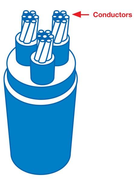
215 Figure 3

216 Figure 4 The proper selection of the cable and the conductors depends on: The expected amperage that will flow through the cable to the motor The calculated voltage drop in the line from the surface to the pump. The space that exists between the tubing collar and the casing (even though the cable is banded to the tubing at selected points, there must be enough space to install and pull the pump without damaging the cable or hanging it in the well). The equipment operating environment - such as the operating pressure and temperature at pump depth.

217 CABLE AMPERAGE The first consideration in selecting cables is amperage. The limits on amperage for cables containing copper conductors are as follows: Cable No. Maximum Amperage Note that the cable with the smaller number has the larger diameter. Thus, a Number 1 cable can carry a maximum of 115 amps. VOLTAGE DROP The second selection consideration is the voltage drop that will occur between the wellhead and the pump. Normally, the maximum voltage drop for an electrical cable is about 30V per 1000 feet. (Figure 5) is a graph of amperage versus voltage drop per thousand feet of cable length for various conductors. Figure 5

218 For example, if a 60-amp current is flowing through a 1000-foot cable, then the voltage drop in a No.1 copper conductor will be about 16 V. In a No.4 copper conductor, it will be about 31V; while a No. 6 copper conductor produces a voltage drop of about 45V. Clearly, the larger conductor with the lower voltage drop is more desirable, especially in deep wells. A counter-argument to this is that the larger cable costs more, and might not fit within accepted tolerances between the tubing collars and the casing. These factors must be anticipated and balanced when designing a system. ESP OPERATING PRINCIPLES In most cases, submersible pumps are installed on tubing, although some are suspended at the end of the power cable so that they can be retrieved without having to pull the tubing. In this section, we will limit our discussion will to downhole pumps installed at the bottom of the tubing. Electrical submersible pumps are multi-staged centrifugal pumps Each stage consists of a rotating impeller and a stationary diffuser (Figure 1: Single stage of a centrifugal pump, showing impeller and diffuser). Figure 1 As the shaft of the pump moves in response to the force of the motor, the impeller turns, causing a rotating motion in the fluid. The diffuser changes the direction and velocity of flow and directs fluid from the impeller of one stage to the impeller of the next stage. The type of stage determines the volume of fluid to be produced. The number of stages contained in a pump determines the total pressure, or head, generated. The horsepower required by the motor is determined by both the volume displaced and the head generated. Pumps are manufactured in a range of capacities to satisfy almost all well conditions. A pump s impellers are designed to operate efficiently over a specific capacity range ( Figure 2: Optimal ESP operating range). Operating the pump below its design capacity causes the impeller to downthrust against the diffuser, resulting in wear on the bearings and washers. Conversely, if the pump operates above its design capacity, the impeller upthrusts against the upper part of the diffuser, causing similar wear. Ideally, the impeller should float freely, and will do so throughout its recommended operating range. This recommended operating range will allow the pump to run at highest efficiency.

219 Figure 2 Pump length and diameter are constrained by manufacturing and wellbore conditions. Assembly and handling difficulties usually limit the length of a single pump section to about 20 to 25 feet. However, it is possible to join pump sections together, adding successive stages to develop the required head. Pump diameters are limited by the size of casing in which they are to be run. Table 3 lists the suggested pump diameters for various casing sizes; for example, a 3 3/8-inch OD pump will fit within 4 1/2-inch OD casing. If the casing diameter is 8 5/8 inches or greater, then larger pumps could be used. Table 3: Recommended ESP diameters for various casing sizes (after Brown, 1980) O.D. of casing Casing weight Motor O.D. Pump O.D inch 11.5 lb/ft 3.75 inch inch 9.5 lb/ft 5 inch All weights 3.75 inch inch 5.5 inch 20 lb/ft 4.5 inch 4.0 inch

220 17 lb/ft 15.5 lb/ft 7 inch 28 lb/ft 4.5 inch 4.0 inch 26 lb/ft 5.5 inch inch 4.5 inch 4.0 inch 5.5 inch inch inch 6.75 inch 24 lb/ft 20 lb/ft inch or greater All weights The number of stages that can be added to a pump are limited by three variables: Horsepower rating of the shaft that turns the pump Pressure rating of the pump housing Capacity of the thrust bearing The pump manufacturer takes each of these variables into account when a customer specifies the capacity range for a pump. ESP SYSTEM DESIGN This section examines the considerations and design procedures involved in selecting a pump and motor for an ESP system, and the steps needed to determine the surface voltage requirements. PUMP PERFORMANCE CURVES In selecting a pump for a particular application, we must look carefully at its performance or test curves, which typically chart three different aspects of performance: head versus pump capacity, motor horsepower versus capacity and pump efficiency versus capacity ( Figure 1: ESP performance curve. Courtesy Schlumberger-Reda.)

221 Figure 1 These curves are published by pump manufacturers for each of their individual pump types the ones shown in (Figure 1), for example, are for a 100 stage, Schlumberger-Reda D1350 pump. They are obtained by running a pump in water at a constant speed, while varying its throughput by throttling the discharge side of the pump. During the test, the pressure difference across the pump, the brake horsepower, and the pump efficiency are measured at different pump throughput rates. The resulting pressure increase is then converted to its equivalent head. With this data, performance curves are drawn showing head, pump efficiency, and brake horsepower for a specified number of pump stages, as a function of pump throughput rate. Although these curves are generated using fresh water (with a specific gravity of 1.0), the same values of head are usually used when selecting a pump for a fluid with a different specific gravity provided the viscosity of the fluid is similar to the viscosity of water. Brake horsepower, on the other hand, does require a specific gravity correction. Pump performance curves are normally published for either a single pump stage or, as was done in Figure 1, for 100 pump stages.

222 PUMP HORSEPOWER REQUIREMENTS Using the pump performance curve shown in (Figure 1) above, we may determine the horsepower requirements for a pump under a given set of operating conditions for example, a flow rate of 1250 B/D and a required pump pressure of 1725 psi. First, we note the following values corresponding to a capacity of 1250 B/D: Head generated for 100 stages = 2280 ft, or 22.8 ft per stage Brake horsepower required = 32.5 hp, or hp per stage Pump efficiency = 64 percent. The number of stages required is: (1) The total head is equal to the required pump pressure divided by the pressure gradient of fresh water (the fluid upon which the pump curve is based), or psi/ft. Therefore, To calculate the required brake horsepower (hp), we multiply the horsepower per stage by the number of stages and by the specific gravity of the fluid being pumped (in this case, the fluid is fresh water, and so the specific gravity is 1.0): hp = (hp per stage) x (stages) x (specific gravity) (2) = (0.325) x (l75) x (1.0) = 56.9 hp In summary, this procedure requires specifying the pump operating conditions (required capacity, in B/D, and the required fluid head). The required capacity of the pump is based on an estimate of the well s inflow performance. The performance curves are actual test curves. If we assume that very little gas will be pumped, we do not need to apply a pump efficiency factor. We should select the pump to provide the desired capacity based on continuous operation. In evaluating the capabilities of various pumps, we may have a number of options from which to choose. It is important to study the performance curves supplied by the manufacturer to select a pump that, at the required capacity, will operate in its optimal capacity range at the highest pump efficiency. Remember that pump capacity depends on the design of the impeller and not on the number of stages. With the selected performance curve and pump capacity, look up or calculate the head/stage and horsepower/stage. Once we know the required head, we can calculate the total number of stages needed and the horsepower required for the motor. TOTAL DYNAMIC HEAD Along with specifying the required capacity of a pump, we need to determine how much total dynamic head (TDH) it must provide. The TDH is the total head required when pumping at the desired rate. It is the difference between the head at the pump discharge and the head at the pump intake. Assuming the produced fluid has no free gas, and that all pressures are converted to head (in feet) using the specific gravity of the produced fluid, TDH is equal to: the head caused by backpressure in the tubing, minus the frictional losses generated by flow in the tubing,

223 plus the head contributed by the liquid column in the tubing, minus the head caused by the operating liquid column in the annulus, minus any head caused by a backpressure imposed on the annulus. Generally, the annulus backpressure is negligible and so the liquid columns may be netted out to give a single term for the net lift. As a rule of thumb, a pump should have at least 500 feet of fluid above it when in the operating mode. As an example, consider a well producing under the following conditions: Tubing backpressure is 75 psi. Pump depth is 8500 ft; operating fluid load depth is 700 ft above the pump. Tubing size is 2 7/8-inch OD; casing size is 7-inch OD. Desired pump rate is 1400 B/D. Fluid being pumped is 25-degree API oil (specific gravity = 0.904; gradient = psi/ft). Assume that there is no packer in the hole Because there is no backpressure on the annulus, the TDH, expressed in feet, can be estimated using the following equation: TDH = head due to tubing backpressure + frictional losses + net lift (3) Tubing backpressure head = The frictional losses during flow in the tubing are obtained using viscosity correlations provided by the pump manufacturer, and are found to be approximately 9 psi per 1000 feet of tubing. This converts to The net lift, with no packer in the hole, is simply the depth to the pump, minus the height of the fluid level above the pump: Net Lift = = 7800 ft When all values are substituted, the total dynamic head is: TDH = = ft This is the value of TDH to use when selecting a pump. MOTOR SELECTION Once we determine a pump s required capacity and TDH, the next step in the design is to review performance curves from different manufacturers. The goal is to (1) select the pump that best meets the capacity needs, (2) calculate the number of stages required, and (3) specify the required motor horsepower. To illustrate, assume the same well conditions that were given in the Total Dynamic Head calculation above, and use the resulting TDH value of 8186 feet. Assume also that after reviewing the performance curves, the pump from (Figure 1) was selected. This pump has an OD of 4 inches and will easily fit within the 7-inch casing. The performance curves for this pump show that at a throughput rate of 1400 B/D and a TDH of 8186 ft:

224 head = 2100 ft / l00 stages hp = 34 hp/100 stages The number of stages and motor horsepower required are as follows: stages = 8186 ft divided by 21 ft/stage = approximately 390 stages hp = (hp / stage) x (stages) x (spec. grav.) = (0.34) (390) (0.904) = approximately 120 hp If the bottomhole temperature is higher than 180 F, the horsepower required should be increased by as much as 20%. In the example well, high temperature is not a limiting factor, so we can go with 120 hp in our design. Next, we need to select a 120 hp motor that will fit into a 7-inch OD casing. In this case, we can go to our manufacturer s catalog and see a listing of 120 HP Series 456 motors with the specifications shown in Table 1. Table 1: 456 Series Motors (4.56-inch OD) 60 Hz HP Volts Amps The Series 456 has an OD of 4.56 inches, which easily fits inside the 7-inch casing. Each of the 120 HP motors listed above has a different required voltage; note that the higher voltage motors require lower current. Now we must select one motor for the application. In general, the choice of motor voltage is a function of line voltage losses, capital costs, and the electric power cost. The required surface voltage is the voltage required by the motor, plus voltage losses between the motor and the surface, including losses in the cable, other system components, and the transformer. The cable losses are the most significant. As an upper limit, cable losses should be less than 30V/1000 ft. If, for example, we select the 1000V, 77-amp motor from Table 1, we can then go to ( Figure 2) (Amperage per voltage drop per 1000 feet of cable, various conductors).

225 Figure 2 We note that an ideal conductor is the No. 2 copper conductor, which at this amperage has a voltage drop of 25V per l000 feet of cable. Another option would be the 2300V, 34-amp motor. This would allow us to use a smaller No. 6 copper conductor and have the same voltage drop along the cable. Because the No. 6 copper conductor is smaller than the No. 2, going with this higher-voltage option would result in a lower capital cost for the cable. However, a higher voltage switchboard will be more expensive than a lower voltage switchboard. We could also consider using a larger conductor cable (for instance the No. 2 copper cable) with the 2300V motor. The voltage loss in the cable will drop from 25V to 11V per 1000 ft. The larger conductor cable will require a higher capital cost, but lower operating costs. Within limits, then, a larger, more expensive cable will allow for lower line losses and thus lower operating costs. In summary, motor selection requires an economic analysis of voltage and cable alternatives; however, the following recommendations should serve as a guide: For low horsepower motors and shallow depths, use a 440V system. For less than 70 hp at intermediate depths, use an 830V system. For 70 to 200 hp in deep wells, use a 1500V system. For motors of 200 volts and greater, use a1500v or 2400V system. The choice of voltages will depend on economics. SURFACE VOLTAGE REQUIREMENTS

226 Before we can select a switchboard and transformer for our ESP system, we must determine the required surface voltage, Vs: (4) V s = V m + ΔV c + ΔV com + ΔV t Where: V s = required surface voltage, volts V m = motor voltage, volts ΔV c = cable voltage losses, volts ΔV com = system component losses, volts ΔV t = transformer voltage losses, volts Consider the 2300V motor for analysis. With the this motor, the No. 1 copper conductor, and a pump depth of 8500 ft, the voltage loss in the cable, ΔV c, is 76.5 volts. Assume the surface component losses, ΔV com, are negligible. The transformer losses, ΔV t, are usually estimated to be 2.5 percent of the required voltage. In this case the required surface voltage without significant electrical component voltage losses and using the No. 1 copper conductor would be: V s = (2376.5) = 2436 V Operating voltage is variable within a 50V range; thus, a standard 2400V transformer system would meet this system s voltage requirements. In most cases, it is better to have a required surface voltage below 2400V. For this reason, we should analyze the other motor and cable options to find one that will provide a surface operating voltage somewhat below that of the transformer system. Further analysis of this specific pump system shows that the 1170V motor with a No. 4 copper conductor cable will require a surface voltage of 1495V. With this pump and cable, we may specify a system voltage of 1500V. The switchboard would have a maximum voltage rating of 1500V and a maximum amp load of at least 66 amps. The transformer size is expressed in kilovolt-amps, kva, and is given by the expression: (5) kva = V s A m Where: kva = transformer size, kv-amps V s = system voltage, V A m = motor amperage, amp For this example, V s is equal to 1495 volts and A m is equal to 66 amps. So the transformer size is: kva = 0.00l73(l495)(66) = 171 KVA If we use three single-phase transformers, each will require one-third of this value, or about 57 kva. Other specifications of the transformer would be determined in consultation with the manufacturer and would include consideration of the primary line voltage available in the operating area (Table 2 ). Table 2: Transformer Specifications Single Phase OISC 60 Hz, 55 (After TRW) Size, Height, Width, Depth, Weight, Delta Primary kva inches inches inches lbs. Volts deg C Rise Delta Secondary Volts / / / / / / / 1300

227 / 1300 PRESENCE OF EXCESSIVE FREE GAS The TDH calculation outlined in this section is accurate if significant volumes of gas are not being pumped, and if no gas is coming out of solution as fluid is produced up the tubing. If gas is present, then additional considerations come into play. Normally the pump is installed on the tubing without a packer. This means that free gas is easily vented up the annulus. (Many ESP well installations--especially offshore--do include packers.) It is not feasible to vent annulus gas to the atmosphere so it must travel through surface flow lines. However, the annulus backpressure and any surface venting must be controlled so that the pump is below an acceptable level or fluid submergence. If not, the pump may become gas-locked. Manufacturers provide downhole gas separators to assist in preventing gas from entering the pump. If the pump is set at a depth at which the pressure is below the bubble point, any free gas that is not separated will be pumped. The pump will perform normally if the volume of free gas is below 10%. If significant gas volumes are present in the fluid, a higher capacity pump will be needed. An offsetting factor is that the presence of gas in the tubing will reduce the TDH and thus reduce the required motor horsepower. All other considerations equal, it is more difficult to size pumps for wells that pump gas, because it becomes necessary to estimate the pressure-volume effects that occur between the pump intake and discharge pressures. This is illustrated in ( Figure 3) (Effect of gas compression on ESP throughput). Note that the initial pump stages perform a substantial amount of gas compression. Between an intake pressure of 500 psi and a discharge pressure of 1215 psi, the fluid volume is reduced almost by half.

228 Figure 3 Handling gas effects in the ESP design generally involves the following steps: 1. Estimate the pump intake pressure from inflow data 2. Estimate the pump discharge pressure from multiphase flow correlations 3. Divide the range of pressure between the inlet and discharge valves into discrete increments and then calculate the pressure-volume changes that occur between increments 4. Calculate the average volume throughput and average fluid gradient, from the pump intake to discharge points, and, with this data, select a pump and then specify the number of stages required using the pump s performance curves. The appropriate calculations are typically incorporated into company and manufacturer ESP design software. You should check on the individual program that you are using to ensure that gas effects are taken into account where appropriate.

229 ESP SYSTEM OPERATION One disadvantage of ESP systems is that the tubing string normally has to be pulled in order to replace the pump or other subsurface equipment (unlike, for example, a free hydraulic pump, a rod pump or a wireline-retrievable gas lift valve). This requires a workover rig, which adds to the cost of well maintenance and repair. Replacement of downhole equipment may become necessary because of failures at the motor, pump or cable (Table 1), or because the pump needs to be re-sized due to changes in the well s inflow performance. Table 1: Common ESP Failures Type of failure Possible causes Motor Excessive motor overload Leak in the protector caused by worn or defective seals Insufficient fluid movement to cool the motor Motor housing corrosion Faulty installation Switchboard problems Lightning Unbalanced electrical system Pump section Downthrust or upthrust wear on the pump bearings Wear caused internally by the pumping abrasives Plugged or obstructed stages caused by deposition or corrosion Twisted shaft caused by starting a pump while the fluids are still moving downward in the pump after shut-down Cable Mechanical damage caused during running or pulling operations Deterioration caused by the downhole environment High temperatures caused by amperage loads If the well s inflow has been increasing, the cost of bringing in a workover rig is relatively easy to justify, because the newly installed pump will pay for itself with the higher production rate. But if the inflow is decreasing, the expense is harder to bear, and the temptation might be to just cycle the pump daily instead of replacing it. The problem with cycling an ESP is that large current surges occur when starting up a high voltage, high horsepower induction motor that is separated from its starter at the surface by five or ten thousand feet of cable. These surges are often five to eight times the normal operating current (in Figure 1, a normal 32-amp current surged to 141 amps at start-up Neely, 1982). This type of starting is referred to as across-the-line starting. Starting and stopping the motor also causes amperage and voltage spikes that can damage or burn out the motor. Normally, only a limited number of stops and starts are possible, so most operators are reluctant to stop and start a submersible pump unless it is absolutely necessary.

230 Figure 1 OPTIMIZING PUMP PERFORMANCE There are several ways to optimize pump performance as the well inflow performance changes. CHANGES TO THE MOTOR AND PUMP If well inflow performance is decreasing and the pump is oversized and continuously running, pump performance can be improved by: Changing the pump. This requires pulling the tubing, losing some production, and buying and installing a new pump. Try to avoid this option. Increasing the backpressure at the wellhead. This will reduce the capacity of the pump. This is also undesirable because of the energy waste and the potential for thrust problems in the pump.

231 The remaining alternatives require modifying the electrical submersible pump system. Cycle the pump and motor. This method eliminates the current surges during start and stop operations. This is similar to what is done with the motor of a rod pumping system. Reduce the motor speed and, thus, the speed of the pump. This is the preferred method of changing the pump capacity. SOFT START/SOFT STOP The surges in current during start and stop operations may be limited by using silicone-controlled rectifiers at the surface starter to provide controlled levels of power at the pump. With these rectifiers, the voltage and amperage are allowed to ramp up or ramp down at acceptable rates over a specified period of time. This type of start and stop control, which provides smooth power flow to and from the motor during stop/start operations, is referred to as soft start and soft stop (Figure 2). Soft-start controllers have been used under field conditions and have demonstrated that pumps may be cycled numerous times without damage (Neely, 1982).

232 Figure 2 VARIABLE FREQUENCY DRIVE Another option for changing the capacity of an electric submersible pump is to install a surface device that can change the voltage frequency supplied to the motor. This device is referred to as a variable frequency generator (VFG), variable frequency drive (VFD) or variable-speed drive (VSD). It is used instead of the standard 50- or 60-Hz motor controller at the surface. As an example, a VFG may be rated at 300 KVA with a frequency range of 36 to 90 Hz. Because the motor speed is proportional to frequency, and the pump speed is equal to the motor speed, a variable speed generator allows the pump to operate at a speed above or below its rated capacity at 60 or 50 Hz. There is an upper limit, though, on pump speed variability. This limit is at the amperage overload condition of the downhole motor. Subject to this limit, a variable frequency generator can be used to increase or decrease pump rates by as much as 20% to 30%, to satisfy changing inflow performance. If greater changes are required, a resizing of the pump will be necessary.

233 Variable frequency generators and variable-speed drives can also provide soft-start protection. Using a VSD to control a pump motor can reduce the strain on the pump shaft and reduce pump damage by slowly ramping-up the motor speed. A number of operating procedures have been developed to make the electrical submersible pump more versatile in its application to a specific well or field. However, the best approach is to carefully design and select a pump for each well based on its own characteristics and assume that the pump will operate continuously. ESP SYSTEM MONITORING AND CONTROL ESP systems are complex and require specific operating conditions with respect to the power, fluid level, fluid content, and gas-liquid ratios. Without proper ESP monitoring, operators cannot tell what is happening downhole, and this lack of monitoring may lead to low efficiency, high lifting costs and frequent repair and replacement. Poor ESP performance can also result from improperly designed pump assemblies. Monitoring and performance analysis can extend the life of ESP pump installations by reducing system down time and the cost of repair and replacement of the pumps. Reducing down time also results in higher production from the well, improved ESP performance and increased profitability. Analysis of ESP performance collected from the wellsite data gives the operator real-time information, historical data, and the ability to optimize the wells from a remote location. Monitoring and comparing changes in ESP performance over time can help identify potential problems and correct them before the ESP fails. Typical components include: Downhole pressure, temperature, and electrical sensors Surface System using well sensor data Remote Terminal Unit (RTU) and communications system Interpretation and Analysis Software DOWNHOLE PRESSURE, TEMPERATURE, AND ELECTRICAL SENSORS A well controller gathers data from downhole sensors that provide measurements of ESP performance. The sensors can also measure data such as pump intake pressure, wellhead pressure, and flow rate. Data of this kind can help identify problems before they become more serious. Pump wear, paraffin or scale buildup, sand production, pump off, and blocked perforations can also be identified by making downhole measurements of changes in current and voltage, power factors, and pump intake pressure. SURFACE SYSTEMS USING WELL SENSOR DATA An ESP surface controller may be connected to the downhole sensors and surface instruments to measure conditions and control the operation of the ESP pump in each well. The operator may want to monitor surface performance parameters such as wellhead pressure, net oil, flow volume, and flowline temperature, among others. The controller can be programmed to automatically adjust pump operations using data from the well sensors. The controller regulates the cycling operations of well so that startup of the well is smooth, reducing stress on the motor and pump, improving pump efficiency, and extending the run life of the system. The controllers can also be programmed to send data from the downhole sensors, motor controller to the remote locations using the RTU. REMOTE TERMINAL UNIT (RTU) AND COMMUNICATIONS SYSTEM

234 The sensor data must be communicated from the well to the operator. A typical ESP monitoring system has a remote terminal unit that sends the sensor data to the operator. The RTU may use radio or telephone modem to transmit wellsite data to the operators office. INTERPRETATION AND ANALYSIS SOFTWARE The software, running on a desktop platform, allows the operator to monitor and set the ESP controller on each well in a field. The ESP monitoring and analysis software allows the operator to control, monitor, track, and report on ESP wells. It provides a means of reporting production parameters, tracking lifting costs and detecting operating problems. Proper monitoring of ESP performance can increase pump life, reduce operating and repair costs and improve profitability. With the analysis of pump performance data, the operator can model reservoir inflow and pump performance so that the pump can run at its highest efficiency. The operator can also simulate the performance of several combinations of pump size, setting depth and production rates. This allows the operator to avoid designs that cause stress on the pump, motor, or cable. ESP SYSTEM DESIGN USING FIELD DATA Observations of ESP performance over a long time are used to design the best pump configuration by modeling various combinations of pumping system equipment. The operator can experiment with parameters such as pump setting depth, production rate, and fluid level to determine how these changes affect well performance. Plunger Lift Systems PLUNGER LIFT OVERVIEW Plunger lift (Figure 1) is the only artificial lift method that relies solely on the well s natural energy to lift fluids. The plunger, traveling inside the tubing, moves upward when the pressure of the gas below it is greater than the pressure of the liquid above it. As the plunger travels to the surface, it creates a solid interface between the lifted gas below and produced fluid above to maximize lifting energy. Any gas that bypasses the plunger during the lifting cycle flows up the production tubing and sweeps the area to minimize liquid fallback.

235 Figure 1 The plunger is a cylinder of slightly smaller diameter than the tubing diameter. The exterior of the plunger can have different types of packing elements to seal against the tubing wall. Plungers may be solid or they may have an internal rod-actuated bypass valve. In addition to the plunger itself, a typical assembly consists of two bumper springs one in the bottom section of the tubing, and the other in a lubricator at the surface and a surface controller to control the travel cycle of the plunger. The plunger cycle consists of three stages (Phillips, 1998): 1. Shut-in: During this stage, the well is shut-in to allow the casing pressure to build to the level required to lift the plunger and the liquid above it. 2. Unloading: The tubing is opened, and the stored casing pressure lifts the liquid and the plunger to surface. 3. Afterflow: With the plunger at the surface, the well is allowed to flow in preparation for the next shut-in period At the end of the afterflow period, the well is shut-in, the plunger falls to bottom, and the casing pressure again begins to build. Plunger lift provides a cost-effective method of artificial lift that can be used to efficiently produce both gas wells with fluid loads and high GOR oil wells. It is the only artificial lift method that uses the natural energy of the well to lift fluids. It can be used to APPLICATIONS

236 Plunger lift has found successful application in a variety of production scenarios, including: Producing high-gor oil wells Increasing production from oil wells with low bottomhole flowing pressures Dewatering gas wells or wells in coalbed methane reservoirs Unloading of wells being converted to gas lift Reducing liquid fallback in intermittent gas lift wells Cleaning wells with paraffin, scale or Improving production in wells with emulsion problems Maintaining production in wells that are awaiting other permanent artificial lift process Producing single-well properties or small fields Advantages Can be used in wells as deep as 10,000 ft TVD. Given a sufficient producing GLR, plunger lift operations require no external gas supply. Because there are few moving parts, the system is easy to service and maintain. Reduces need for hot-oiling or mechanical paraffin cutting Works well in deviated wells (if the plunger operates in a relatively straight part of the well) Disadvantages At low velocities ( ft/min), the plunger may stall in the tubing. High velocities ( ft/min) may reduce fluid recovery (more fluid fallback). The plunger also may be damaged if it hits the upper bumper spring too fast. (Optimum plunger velocity is 800 to 1,000 ft/min. The plunger velocity can be estimated by measuring how long it takes the plunger to arrive at the surface after the time-cycle controller opens and gas injection begins. Average plunger velocity can be determined by calculating the depth of the well, divided by the travel time.) TYPES OF PLUNGER INSTALLATIONS Conventional plunger lift without a packer is typically used in wells that have enough formation gas to lift the fluid. This is the most common type of plunger lift installation. Intermittent gas lift using a plunger is for wells with low bottomhole pressure. In this case, the height of the fluid column allows gas to break though during the lift cycle. The plunger keeps the gas and fluid separated, thus reducing fall back while increasing fluid inflow. The gas required for moving the plunger is injected from the surface. Plunger lift with a packer is for gas wells or high-glr oil wells, and uses a packer set in the tubing-casing annulus. When the plunger reaches the surface, it is held there to allow fluid flow to the sales line. In these wells, timers normally control the injection cycle so that the plunger will remain at the surface for a sufficient length of time. PLUNGER LIFT DESIGN AND INSTALLATION Plunger lift can be easily installed in a well using wireline, so it is usually not necessary to pull the tubing. A typical plunger installation is shown in (Figure 1) (Courtesy Weatherford International Ltd).

237 Figure 1 To stop the plunger when it falls to the bottom, a tubing stop and bumper spring assembly are set by wireline at the bottom of the tubing string. This bumper spring is positioned just above the perforations. In wells with low permeability producing formations, a standing valve may be installed below the perforations, between the tubing stop and the bumper spring. At the surface, a lubricator above the master valve contains: a flow outlet, a bumper spring and striker pad to stop the moving plunger, and a catcher to hold the plunger so it can be removed for service. A device to detect the arrival of the plunger is also part of the control system. The arrival of the plunger at the surface closes the gas injection control valve. MECHANICAL EQUIPMENT The main components of a plunger lift system are the plunger, bumper springs, lubricator, controller and the surface gas injection facility. Plungers are manufactured in various diameters, lengths, and temperature ratings to accommodate specific fluid compositions and well conditions. Plungers may be solid or may have a rod-actuated internal bypass valve. Solid plungers fall back to the bottom slowly and are used in wells with longer cycle times. Plungers with a bypass valve are used in wells with shorter cycle times where it is important for the plunger to fall to the bottom more quickly. When the plunger is on bottom, the bypass valve is closed, to keep gas from flowing through it. When the plunger arrives at the surface, the valve rod strikes a bumper spring and pad in the lubricator, thus opening the valve and allowing it to fall to the bottom. At the bottom, the rod contacts the lower bumper spring and pad and closes the valve for the next injection cycle.