MIKE 21. Boussinesq Wave Module. Step-by-step training guide

Transcription

1 MIKE 21 Boussinesq Wave Module Step-by-step training guide MIKE 2017

2 DHI headquarters Agern Allé 5 DK-2970 Hørsholm Denmark Telephone Support Telefax mike@dhigroup.com mike21bw_step_by_step_guide.docx/hkh/ DHI

3 CONTENTS MIKE 21 Boussinesq Wave Module Step-by-step training guide 1 Introduction Background Objective of Training Guide Creating the Bathymetry General Considerations before Creating a Bathymetry Creating the Kirkwall Marina Bathymetry Creating a batsf-file from raw xyz data Initial preparations for creating a sponge layer map Initial preparations for creating a porosity layer map Visualisation of the Bathymetry Creating the Input data to MIKE 21 BW Creating a Sponge Layer Map Creating a Porosity Layer Map Creating Internal Wave Generation Data MIKE 21 BW Model Setup Editor Basic Parameters Calibration Parameters Output Parameters Deterministic parameters Wave disturbance parameters Execution Results Presentation and Analysis Deterministic Results Statistical Results Further Analysis Comparison between MIKE 21 BW and Physical Model Test Data Model Setup Model Results Comparison i

4 MIKE 21 ii Boussinesq Wave Module - DHI

5 Introduction 1 Introduction This MIKE 21 BW step-by-step training guide relates to the Kirkwall Marina located at the bottom of Bay of Kirkwall, Orkney Islands, UK. Figure 1.1 shows the location of the site. Figure 1.1 Kirkwall Marina is located in the Orkney Islands, UK (longitude W ' and latitude N ') 1.1 Background The breakwaters of the Kirkwall Marina have recently been extended with the intention of providing improved wave protection (Figure 1.2). Subsequent operation of the marina has shown the wave conditions to be more severe than anticipated. DHI was commissioned by Orkney Islands Council to investigate the effect of a new breakwater with the aim of improving the wave protection within the marina. The study performed by DHI (April 2005) was based on a three-dimensional (3D) physical model constructed in one of DHI s wave basins. During the study, tests were performed with the existing marina and also with the marina after construction of an extension of the western breakwater, see Figure

6 MIKE 21 Figure 1.2 Arial image of the Kirkwall Marina during the construction of the breakwater extension. Image provided by Orkney Islands Council Figure 1.3 Photo of the 3D breakwater model testing at DHI (left panel) and construction of the new breakwater extension (right panel), August Images from In this step-by-step training guide, the Kirkwall Marina layout from May 2005 will be used as case. The guide also includes a comparison between numerical wave simulation results and results from the 3D physical model. DHI is appreciative of the support of Orkney Islands Council and the Council s permission to use the Kirkwall Marina case in this step-by-step training guide. 2 Boussinesq Wave Module - DHI

7 Introduction Figure 1.4 Arrangement of pontoons in the Kirkwall Marina, May Image from Objective of Training Guide The main objective of this training guide is to set-up a MIKE 21 Boussinesq Wave model for the Kirkwall Marina from scratch, and to simulate the wave disturbance conditions in the Kirkwall Marina. In addition, the simulated results are compared to physical model test results. The files used in this Step-by-step training guide are a part of the installation. You can install the examples from the MIKE Zero start page. Please note that all future references made in this Step-by-step guide to files in the examples are made relative to the main folders holding the examples. User Guides and Manuals can be accessed via the MIKE Zero Documentation Index in the start menu. Success in perception of the information presented in this document (and the user guide) together with the user s general knowledge of wave hydraulics, marine engineering and experience in numerical modelling is essential for getting the maximum benefit from the state-of-the-art tool MIKE 21 BW. 3

8 MIKE 21 4 Boussinesq Wave Module - DHI

9 Creating the Bathymetry 2 Creating the Bathymetry Providing MIKE 21 BW with a suitable model bathymetry is essential for obtaining reliable results. Setting up the bathymetry requires more than just specifying a 2D array of accurate water depths covering the area of interest. It also includes the appropriate selection of the area to be modelled, the grid spacing, location and type of boundaries, etc. When setting up the bathymetry for a MIKE 21 BW simulation, it should be kept in mind that the water depths determine which wave conditions that can be modelled. The maximum water depth restricts the minimum wave period that can be modelled, and the minimum water depth may restrict the wave height, if wave breaking is not included. Further, shallow water depths result in small wave lengths, which imply a small grid spacing which again results in increased computational time. Therefore, it is sometimes necessary to modify the bathymetry to reach an acceptable compromise between a correct bathymetry and correct wave conditions. 2.1 General Considerations before Creating a Bathymetry We are interested in determining the wave disturbance conditions in the Kirkwall Marina for the following offshore conditions (at 12 m depth Chart Datum (CD), see Figure 2.1): Significant wave height, H m0 = 1.9 m Spectral peak wave period, T p = 5.5 s Mean wave direction, MWD = 360 N Standard JONSWAP frequency spectrum Directional and unidirectional wave distributions The water level is corresponding to Mean High Water Spring tides (MHWS), which is +3.0 m CD. A chart of the area of interest is shown in Figure 2.1. It covers the Bay of Kirkwall and the Kirkwall Marina. A rectified version of this image is included in the example folder (file name Rmap1.gif). The rectification is made using the Image Rectifier included in your DHI Software installation. Please select Image Rectifier from the Start menu.. The variation in the water depth in the Bay of Kirkwall is large and will therefore affect the wave propagation and transformation, it is necessary to place the offshore boundary away from the area of main interest (Kirkwall Marina). Further, it is desirable to have the offshore boundary in an area with a relatively small water depth variation. Figure 2.2 shows the location of the anticipated model domain. The size of this domain is approximately 2.3 km x 2.0 km. Next step is to decide the spatial resolution of the model bathymetry. The MIKE 21 BW Model Setup Planner Java Script embedded in the Online Help is a very helpful tool in that process. You can e.g. get access to this tool from the main Help Topics in the MIKE Zero shell: Open MIKE Zero from the Start menu, then click on Help Help Topics and search for the index MIKE 21 BW Model Setup Planner. Click on the link MIKE 21 BW Model Setup Planner and the tool will appear, see Figure 2.3. In the left part of Planner dialogue you enter the requested values and subsequently calculate the estimated simulation time (A), calculate the default upper model limits (B) and correct/evaluate the upper limits (C). 5

10 MIKE According to Figure 2.2 and Figure 2.3, the maximum water depth in the model area is approximately 12.5 m CD at the offshore boundary. On top of that you need to add the water level of +3.0 m. Thus, the maximum water depth is approximately 15.5 m. 2. Theoretically the minimum water depth is 0 m. However, as we will not include wave breaking in this simulation, the minimum depth should be set to a depth such that wave breaking does not occur. The minimum water depth is set to 2.75 m as a compromise between resolving the waves in shallow water areas and to avoid wave breaking in these areas, see also Section The model extent in x-direction is approximately 2300 m. This distance is used for assessment of the required CPU time and RAM demand. 4. The model extent in y-direction is approximately 2000 m. This distance is used for assessment of the required CPU time and RAM demand. 5. The percentage of water area compared to the model domain area is estimated to approximately 60%. This number is used for assessment of the required CPU time and RAM demand. 6. The maximum distance for wave propagation is taken as the distance from the offshore boundary to the innermost part of the marina and is estimated to 2300 m. 7. The time required for calculation of wave statistics (wave heights) in the model domain is set to 20 minutes (default). This time period is usually sufficient to obtain a statistically stable estimate for the significant wave height (or wave disturbance coefficient) in short period related wave problems. 6 Boussinesq Wave Module - DHI

11 Creating the Bathymetry Figure 2.1 Chart covering the area of interest: Bay of Kirkwall and Kirkwall Marina. A rectified version of this image is included in the folder:.\mike_21\bw\kirkwall_marina\data\bathymetry\rmap1.gif 1. The computational speed depends on your hardware etc. and can be found at the end of the simulation run log file. The speed is estimated to 400,000 points/second. This number is used for assessment of the required CPU time. 2. The spectral peak period is 5.5 s in this case. This value is also used for assessment of the required CPU time. Now you can calculated the required total simulation time (Part A), which equals a startup period (i.e. the time required for the waves to propagate from the internal generation line and into the harbour) and the time required for calculation of wave statistics. The estimate is 27.5 minutes, see Figure 2.3. Next is to calculate the default upper limits for the spatial and temporal resolution. As you need to resolve the most energetic components in the wave spectrum (wave periods 5.5 s), the calculation shows that you have to use the so-called Enhanced Boussinesq equations (same as including the so- 7

12 MIKE 21 called deep water terms in the model). Based on the suggested values 1, we choose following parameters: Minimum wave period, T min = 4.5 s Spatial resolution (or grid spacing), x= 3m Temporal resolution (or time step), t= s Change the default values in the own suggestion -dialogues and press the Update upper limits using T min and check/evaluate. The result is shown in Figure 2.3. The Planner estimates the CPU time to be approximately 2.8 hours and the simulation requires approximately 50 MB of internal memory (RAM). Figure 2.2 Definition of MIKE 21 BW model domain 1 The formulas for estimating the minimum wave period and the temporal and spatial resolution are described in the MIKE 21 BW User Guide and in the Online Help. A link is provided in the Notes section in the MIKE 21 BW Model Setup Planner. 8 Boussinesq Wave Module - DHI

13 Creating the Bathymetry Figure 2.3 MIKE 21 BW Model Setup Planner for the Kirkwall Marina simulations 9

14 MIKE Creating the Kirkwall Marina Bathymetry Creating a batsf-file from raw xyz data The bathymetry is created using the MIKE Zero tool Bathymetry Editor. Open MIKE Zero from the Start menu and then click File New File, see Figure 2.4. Figure 2.4 Bathymetry Editor in MIKE Zero Double-click on and a Define Working Area dialogue appears. As map projection, please select OSGB (Ordnance Survey of Great Britain). The map projection and ellipsoid parameters can be found MIKE Zero File Options Edit Map Projections. The extension of the working area is indicated in Figure 2.5. Figure 2.5 Bathymetry Editor (Define Working Area dialogue) After entering the figures click OK and the work space area appears (see Figure 2.6). 10 Boussinesq Wave Module - DHI

15 Creating the Bathymetry Figure 2.6 Bathymetry Editor - work space area (OSGB coordinates) The next step is to add the rectified image (file name Rmap1.gif) as a background image. Click on Work Area Background Management (or simply use the shortcut Ctrl B) and import the correct file. Click OK and then click on Work Area Show Background Images, see Figure 2.7. Figure 2.7 Bathymetry Editor - work space area with background image 11

16 MIKE 21 It is now time to save all the settings. File Save As...(or just use the shortcut Ctrl S). Save the data in folder.\kirkwall_marina\data\bathymetry and using the proposed file name Bat1.batsf. Please note when this file is re-loaded again into MIKE Zero (e.g. by drag and drop) the background image is not shown as default. Please click on Show Background Images as illustrated in Figure 2.6. Based on the chart (rectified image Rmap1.gif), xyz data for the land and water can be obtained by digitalisation. However, in this example xyz data have already been prepared. In the.\kirkwall_marina\data\ascii-folder, the file land.xyz includes polygons for the land and shoreline and the water.xyz file includes the water depths. Import the digitised shoreline data (land.xyz) and digitised water data (water.xyz) from ASCII files, see Figure 2.8. Remember to convert from OSGB co-ordinates (WorkArea Background Management Import). When you have imported the two files into the workspace you will see a working area as shown in Figure 2.9. Figure 2.8 Import the digitised land and water xyz data 12 Boussinesq Wave Module - DHI

17 Creating the Bathymetry Figure 2.9 Working Area after import of land and water data The next step is to define the bathymetry. Click on Work Area Grid Bathymetry Management New (or use the shortcut Ctrl M). Specify the bathymetry as follows, cf. Figure 2.10: Grid spacing 3 m in both directions Origin in m East and m North Orientation Number of grid points 751 in x-direction and 676 in y-direction Land value 10m Please note: As the convergence (defining the angle between the longitude and the UTM northing line) is calculated to 0.82 (using e.g. Grid Plot in the Plot Composer), the orientation is set to degrees in order to ensure that the model has a true north-south alignment. The working area will now look like the one illustrated in Figure

18 MIKE 21 Figure 2.10 Define Bathymetry Area Figure 2.11 Working Area with imported depth values and defined bathymetry (the black rectangle) 14 Boussinesq Wave Module - DHI

19 Creating the Bathymetry The next step is to import data from background. Click on the Import from Background icon in the toolbar and drag the mouse over the points of interest. Selected points are now changing colour. Finally, click on Import from Background once more. Now you are ready for interpolation of the xyz data to grid points. Click on Work Area Grid Bathymetry Management Interpolate, see Figure After the interpolation, the bathymetry is saved into Bat1_0.dfs2 (after you save the Bathymetry Editor specifications into Bat1.batsf, use e.g. shortcut Ctrl S).You may also save the grid file into another file name. In that case you click on the Export -button and specify the file name. Figure 2.12 Imported data from background (red squares) and interpolation to the define grid (the black rectangle) The next step is to load the created bathymetry file (Bat1_0.dfs2) 2 into the MIKE Zero Grid Editor for visualisation and further modification. When a MIKE Zero shell is open simply drag and drop the.dfs2-file into the shell, see Figure An identical.dfs2 file is already included in the DHI Software installation, see.\kirkwall_marina\data\bathymetry\bathy_v01.dfs2 15

20 MIKE 21 Figure 2.13 Grid Editor showing the interpolated bathymetry For QA purposes you may use the rectified chart as an overlay in the Grid Editor. Click on Data Overlay (in menu bar) Add/Remove Layers and load the Rmap1.gif file. Edit the image style parameters as shown in Figure The overlay drawing order is defined in the Overlay Manager, see Figure Finally, change the colour scale as shown in Figure 2.16, View Palette New. Figure 2.14 Image styles parameters (in Image Manager) for the image file Rmap1.gif file 16 Boussinesq Wave Module - DHI

21 Creating the Bathymetry Figure 2.15 Overlay drawing order (in Overlay Manager) for the image file Rmap1.gif file Figure 2.16 Changing of colour palette in the Grid Editor 17

22 MIKE 21 Figure 2.17 Setting colour palette in the Grid Editor the three steps With these settings the bathymetry is visualised as shown in Figure Now it is easy to modify the land/water boundary where the interpolated results are not entirely in agreement with the chart. The settings are automatically saved into a so-called Grid State File (.gsf) 3, see Figure Next time you reload the Bathy_v01.dfs2 file the settings will appear automatically. 3 An identical.gfs file is already included in the MIKE Powered by DHI software installation, see.\kirkwall_marina\data\bathymetry\bathy_v01.gsf 18 Boussinesq Wave Module - DHI

23 Creating the Bathymetry Figure 2.18 Bathymetry with a chart overlay in the Grid Editor Figure 2.19 When saving the dfs2 file the Grid Edit settings will be save a Grid State File (.gsf file) As the water level in the simulation is +3.0 m CD, you have to increase the water depth in the bathymetry. Click on Tools Select Values as illustrated in Figure Select values as shown in Figure Now click on Tools Calculator and add 3 m to all the selected points, see Figure Please note that the depths at the tidal flats are selected, also. Now save the changes into a new.dfs2-file, e.g. Bat2_0.dfs2. 19

24 MIKE 21 Figure 2.20 Select Values Step 1 Figure 2.21 Select Values Step 2 The next step is to set the minimum water depth to 2.75 m. In other words, all depths less than 2.75 m should be set to m in the bathymetry. Please use the same procedure as described above. Figure 2.23 shows the selected points where the water depth is set to Boussinesq Wave Module - DHI

25 Creating the Bathymetry Figure 2.22 Add the 3 m to the selected bathymetry grid points Figure 2.23 Select area where the depth is less than m In most MIKE 21 BW applications, the input wave conditions are imposed through internal wave generation. This is performed by adding the discharge of the incident wave field along the specified wave generation lines. One of the advantages of using internal generation is that absorbing sponge layers can be placed behind the generation line, to fully absorb waves leaving the model domain. This means that all open boundaries need to be closed, i.e. adding an artificial land value to the open boundary. 21

26 MIKE 21 Open the generated bathymetry file Bat2_0.dfs2 in the Grid Editor (simply drag and drop the file from the Windows Explorer to the MIKE Zero shell) and change the water value along the open boundaries to value 5 by editing, see Figure Initial preparations for creating a sponge layer map In Section 3.1 you will learn how to create a sponge layer map based on the bathymetry file and other parameters. Basically a sponge layer covering 20 grid points will be included in the sponge layer map along all bathymetry grid points having a value of 5. Figure 2.24 Close all open boundaries by adding a value of 5 to the bathymetry Absorbing sponge layers may also be used in coastal areas where wave breaking may take place and where wave breaking is excluded in the simulation. In the present case we will apply a sponge layer along a short stretch of the coastline near the eastern offshore part of the model domain, see Figure This trick will ensure a more stable numerical solution in this area and reduce the risk for a model blowup caused by not including wave breaking. Therefore, the land value at the shoreline has been changed from 10 to 5 along the section where a sponge layer is needed. Please load the file Bathy_v02.dfs2 (located in the folder.\kirkwall_marina\data\bathymetry) into the Grid Editor and inspect the changes. This modification will neither affect the simulated wave conditions in the Bay of Kirkwall nor the conditions inside the marina. 22 Boussinesq Wave Module - DHI

27 Creating the Bathymetry Figure 2.25 Change of land values from 10 to 5 along the shoreline where a sponge layer will be included Initial preparations for creating a porosity layer map A porosity layer map is used to model either partial reflection and/or transmission through various types of structures. If porosity values are backed up by land, partial reflection will take place. In Section 3.2 you will learn how to generate a porosity layer map based on the bathymetry file and other parameters. However, the initial preparations usually start when setting up the bathymetry. The typical procedure is to change the bathymetry value from the initial land value (10 in this case) to another (code-) value, e.g. 8, along all structures having partial reflective properties. As seen from Figure 1.2 and Figure 2.26 most structures inside Kirkwall Marine are vertical impermeable breakwaters with almost fully wave reflective characteristics. The inner part of the marina is protected by rock armour at a slope of 1:1.5 to 1:5. Therefore, the bathymetry value (10) along the shoreline has been modified to 8, see Figure Similar modifications are included in the file Bathy_v02.dfs2 reflecting areas where partial reflection is occurring, see Figure The final bathymetry file has now been created and is ready for use. So far we have only used the Grid Editor to view and edit the file. Other alternatives for visualisation are the MIKE Zero s Plot Composer and MIKE Animator Plus, as illustrated in Section

28 MIKE 21 Rock armour Rock armour Wave absorber Figure 2.26 Aerial images from Kirkwall Marine. Images provided by Orkney Islands Council 24 Boussinesq Wave Module - DHI

29 Creating the Bathymetry Figure 2.27 Change of land values from 10 to 8 along the shoreline inside the Kirkwall Marina where a porosity layer will be included for modelling of partial reflection Figure 2.28 The orange colour indicates areas where partial reflection occurs and where a porosity layer will be included in the simulation 25

30 MIKE Visualisation of the Bathymetry The Plot Composer included in MIKE Zero is a good tool for 2D visualisation, presentation and QA of the generated bathymetry. To make a plot of the bathymetry open the Plot Composer, see Figure Figure 2.29 Starting the Plot Composer in MIKE Zero Click on Plot in the menu bar (or use the shortcut Ctrl I) Insert a Plot Object and select Grid Plot, see Figure Figure 2.30 Insert a new plot object as Grid Plot in the Plot Composer 26 Boussinesq Wave Module - DHI

31 Creating the Bathymetry Next, load the bathymetry file Bathy_v02.dfs2 (located in the folder.\kirkwall_marina\data\bathymetry), see Figure Click OK and the first visualisation attempt appears, see Figure Figure 2.31 Load the bathymetry file in Grid Plot Figure 2.32 First attempt on visualisation of the bathymetry 27

32 MIKE 21 Now you can right-click on the plot area to select and change the properties of the plot. Before leaving the Plot Composer, please save the plot specifications into a file (file extension.plc). We have prepared at Plot Composer file for you. Please drag and drop the file MzPlot_Bathy_v01.plc (included in the folder.\kirkwall_marina\data\bathymetry) into the MIKE Zero shell. The result is shown in Figure For QA purposes you may use the rectified chart (the Rmap1.gif) as an overlay in the Grid Plot. The procedure is; right-click on the plot area and click on Add/Remove Layers. The subsequent steps are identical to the overlay management procedure used in the Grid Editor, see Figure As illustrated in Figure 2.34, you may zoom in on various areas for a detailed comparison (and QA) between the generated bathymetry and the chart. Figure 2.33 Plot Composer after loading the file MzPlot_Bathy_v01.plc included in the installation 28 Boussinesq Wave Module - DHI

33 Creating the Bathymetry Figure 2.34 Zoom in on Kirkwall Marina for a comparison between generated bathymetry and chart data Any of the illustrated images can be saved to the clip board as an enhanced meta file (ewf) or as an image file (png, bmp, jpg and tif). You simply right-click on the plot area and select the required output format from the context menu. The images are ready for use in your reports, web sites, etc. An example is shown in Figure For 3D visualisation, the MIKE Animator Plus 4 included in MIKE Zero is a unique tool. To make a plot (or an animation) of the bathymetry, please select MIKE Animator Plus from the Start menu, see Figure The next step is to load the bathymetry file (Bathy_v03.dfs2 5 ) into a MIKE Animator Plus project. Click on Insert in the menu bar and Scene and select the Bathymetry variable, see Figure 2.37 and Figure Please note that MIKE Animator Plus is not included in the general MIKE 21 Pre- and Post-processing package and requires a separate license. 5 The file Bathy_v03.dfs2 is identical to Bathy_v02.dfs2 except that all land values have been multiplied by a factor of 0.1 (using the Grid Editor) for a smoother transition between water and land values. 29

34 MIKE 21 Figure 2.35 PNG-image (2000 x 1500 pixels) of the Kirkwall Marina bathymetry (Bathy_v01.dfs2) Figure 2.36 Starting MIKE Animator Plus 30 Boussinesq Wave Module - DHI

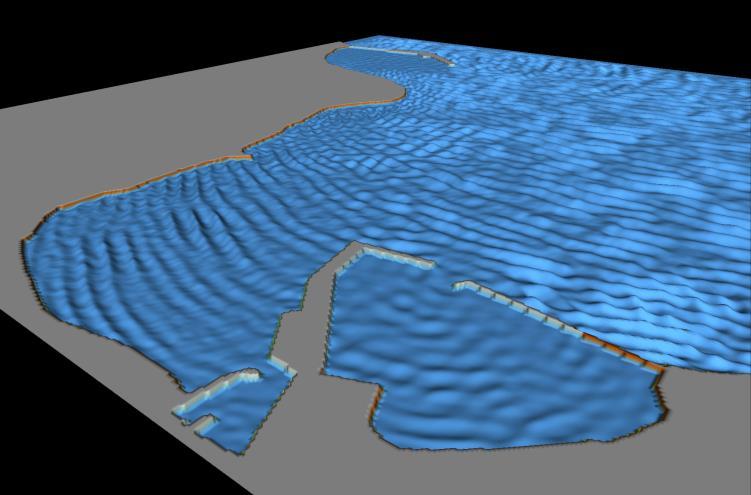
35 Creating the Bathymetry Selecting the Scene mode under the image and moving the mouse will allow you to change the view point. Using this procedure provides a quick way of inspecting and approving the bathymetry. You can also change the focus point, colour scale, distortion, saving images, etc. by using the many features included in the MIKE Animator Plus, see Figure Figure 2.37 Add files to a MIKE Animator Plus project Figure 2.38 Initial 3D view of the bathymetry file Bathy_v03.dfs2 You should remember to save the specifications (extension.lyt) before leaving the tool. Use e.g. the shortcut Ctrl S. 31

36 MIKE 21 Figure D view of the bathymetry in front of the Kirkwall Marina (file Bathy_v03.dfs2) 32 Boussinesq Wave Module - DHI

37 Creating the Input data to MIKE 21 BW 3 Creating the Input data to MIKE 21 BW Before the MIKE 21 BW model can be set up, the following input data must be prepared: Sponge layer map (for wave absorbing) Porosity layer map (for partial wave reflection) Internal wave generation data (for incident offshore waves) Preparation of these data is made by using various tools in MIKE 21 Toolbox. Reference to the MIKE 21 Toolbox User Guide is available in the Manuals folder:.\mike_21\toolbox\m21toolbox.pdf 3.1 Creating a Sponge Layer Map In Section we made the initial preparations for creating a sponge layer map by modifying the bathymetry land value in areas where an absorbing sponge layer is required. The sponge layer map is usually created using the MIKE 21 Toolbox. Open MIKE Zero, Ctrl N and click on MIKE 21 Toolbox, see Figure 3.1. Double-click on the MIKE 21 Toolbox Waves Generate Sponge and Porosity Layers Maps and a wizard appears, see Figure 3.2 and Figure 3.3. Figure 3.1 Select MIKE 21 Toolbox 33

38 MIKE 21 Figure 3.2 Tool for (initial) generation of sponge and porosity layer maps Figure 3.3 Start page of wizard for generation of sponge and porosity layer maps You may change the setup name to e.g. Sponge (Figure 3.3). Click Next and select the input file, i.e. the bathymetry file Bathy_v02.dfs2, see Figure 3.4. After loading the file, click Next. On the next wizard page you should keep the default selected area (entire model domain) and type 5 in the Add values along code value box. In this case, a 34 Boussinesq Wave Module - DHI

39 Creating the Input data to MIKE 21 BW sponge layer will be added along all stretches with a code value of 5. Allow Include corners in search. Figure 3.4 Select the input file for creating the sponge layer map, i.e. the bathymetry file we prepared in Section Figure 3.5 Specification of sponge layer coefficients 35

40 MIKE 21 Very good wave absorbing characteristics are obtained for a sponge layer width of one to two times the wave length corresponding to the most energetic waves. As the maximum depth is 15.6 m and the spectral peak wave period is 5.5 s, the corresponding wave length is approximately 46 m near the offshore boundary. Hence, a width of 20 sponge layers is sufficient in this case. Please insert this number in the open dialogue box, see Figure 3.5. The Online Help (press F1) includes a table of recommended sponge layer parameters depending on the selected number of layers, cf. Figure 3.6. For 20 sponge layers, the base value is a= 7 and the power value r= 0.7, see Figure 3.5. The background value (the sponge coefficient used at open water points where no absorption takes place) should always be set to one (1). Click Next when you have inserted the correct numbers. Figure 3.6 Online Help showing the recommended sponge parameters as function of the number of sponge layers On the next wizard page you should specify the file name of the sponge layer map (e.g. My_Sponge_Map1.dfs2), see Figure 3.7. Click Next to go to the last page and here you click on the Execute button, and when the calculations are finished, a small Run Engine status dialogue appears, see Figure 3.8. Here, you click OK. Please note: Before leaving the MIKE 21 Toolbox, you should save the specifications (Ctrl S), e.g. My_Input_setup1.21t in the folder.\kirkwall_marina\model_setup_1 6. The next step is to check and approve the generated sponge layer. Drag and drop the sponge file into the shell (the Grid Editor opens the file), see Figure 3.9. Move the cursor to the offshore boundary and check the sponge layer here. As expected, 20 sponge layers have been put in front of the offshore (artificial) land boundary. Alternatively, you may use Grid Plot in the Plot Composer. Please drag and drop the file MzPlot.Sponge.plc (included in the folder.\kirkwall_marina\model_setup_1, see Figure The file Input_setup1.21t (in folder \Model_setup_1) is included in the installation and covers specifications of the sponge, porosity and internal wave generation data. Your generated sponge layer file should be identical to the file Sponge_Layer_Map1.dfs2 also included in the installation (in folder.\kirkwall_marina\data\sponge) 36 Boussinesq Wave Module - DHI

41 Creating the Input data to MIKE 21 BW Figure 3.7 Specifying the location and name of the sponge layer map Figure 3.8 Run Engine Status dialogue 37

42 MIKE 21 Figure 3.9 Sponge layer map near the offshore boundary (using Grid Editor tool) Figure 3.10 Sponge layer map using Grid Plot in the Plot Composer 38 Boussinesq Wave Module - DHI

43 Creating the Input data to MIKE 21 BW The sponge layer map can be saved as an image file and be imported into your report. You simply right-click on the plot area and select the required output format from the context menu. An example is shown in Figure 3.11, where the orange area indicates the absorbing sponge layer. Figure 3.11 PNG-image (1000 x 861 pixels) of the Kirkwall Marina sponger layer map (Sponge_Layer_Map1.dfs2) 3.2 Creating a Porosity Layer Map In Section we made the initial preparations for creating a porosity layer map by modifying the bathymetry land value in areas where partial wave reflection occurs. The porosity layer map is created using the following two tools in the MIKE 21 Toolbox (wave section): Calculate Reflection Coefficient Generate Sponge and Porosity Layers Maps The governing Boussinesq equations in MIKE 21 BW have been modified to include porosity and the effects of non-darcy flow through porous media. In this way it is possible to model partial reflection, absorption and transmission of wave energy at porous structures such as rubble mound breakwaters. Thus, the primary task in creating a porosity layer map is to estimate the porosity value using the MIKE 21 Toolbox program Calculate Reflection Coefficient. The procedure is described below (see also the User Guide for the MIKE 21 Toolbox). 39

44 MIKE 21 Step 1 Step 2 The first step is to change the bathymetry value from the initial land value to another (code-) value along all structures having partial reflective properties. This was made in Section 2.2.3, see Figure The second step is to estimate the porosity along all structures using the MIKE 21 Toolbox program Calculation of Reflection Coefficients. As the model porosity depends on the porous structure, wave reflection and local wave and depth conditions, the porosity is basically a model calibration parameter. The model domain is usually divided into a small number of areas with the same porosity. In the present case, we have selected four areas where partial wave reflection occurs as depicted in Figure 3.12, see Table 3.1 The areas 3 and 4 are in the inner part of the marina and are protected by rock armour at a slope from 1:5 to 1:1.5, see Figure Please note that the wave agitation is expected to be higher in area 3 than in area 4. Table 3.1 Selected areas with different model porosities Area number in Figure 3.12 Type of structure Estimated reflection coefficient R 1 Rocky beach, rock armour, see Figure Wave absorber (Shed units), see Figure Rock armour, see Figure 2.26, Figure 1.2 and Figure 2.26, slope 1:1.5 4 Rock armour, see Figure 2.26, Figure 1.2 and Figure 2.26, slope 1: Both the eastern and western breakwaters are modelled by impermeable walls, with the nearshore part of the eastern breakwater protected by rock amour, see Figure Before we calculate the porosity values for the selected areas, a rough estimate of the waves and depths are required for the four areas, see Table 3.2. The wave disturbance coefficient (or relative wave height) is estimated based on experience and diffraction diagrams 7. The incident offshore wave height is taken as H m0 = 1.5 m, see also Figure Alternatively, a quick rough estimate of the wave disturbance can be obtained from a simulation using a porosity map with a constant porosity along all porous structures. The results of this simulation (relative wave height distribution) can subsequently be used for an improved estimate of the porosity. 40 Boussinesq Wave Module - DHI

45 Creating the Input data to MIKE 21 BW Figure 3.12 Areas with different reflective characteristics Now, the next step is to open MIKE Zero, Ctrl N and click on MIKE 21 Toolbox. Doubleclick on the MIKE 21 Toolbox Waves Calculation of Reflection Coefficients and a wizard appears, see Figure You may change the setup name to Area 1. Click Next and specify the relevant wave theory (MIKE 21 BW in this case). Enter the wave height, wave period and water depth from Table 3.2, corresponding to a water disturbance coefficient of 0.8, see Figure

46 MIKE 21 Table 3.2 Estimated wave and water depth conditions Area number in Figure 3.12 Wave disturbance coeff. k (-) Wave height H m0 (m) Wave period T p (s) Water depth h (m) Figure 3.13 MIKE 21 Toolbox tool for calculation of porosity values, Area 1 42 Boussinesq Wave Module - DHI

47 Creating the Input data to MIKE 21 BW Figure 3.14 Specification of wave theory and estimated wave conditions for the selected area Figure 3.15 Specification of porosity layer parameters 43

48 MIKE 21 On the next wizard page you should specify the parameters for the porosity layer, see Figure The width of the absorber should usually correspond to the width of the porosity layer used in your wave model set-up. The width should not be less than approximately 25% of the characteristic wave length in order to be efficient. In the present case we use 3 porosity layers, i.e. the width is 9 m as the grid spacing is 3 m. This corresponds to approximately 35% of the wave length corresponding to the spectral peak wave period. For the diameter of stones and the laminar and turbulent resistance coefficients you should use the default values. Only if you have a specific reason for using custom values, these parameters should be changed. Make sure you are using the same parameters in the MIKE 21 BW (see Figure 4.20). All the porous structures in this case have an impermeable core. Hereafter, you should specify the range of the porosities for which the reflection coefficient is calculated. Use the default parameters as shown in Figure Finally, you have to specify a file name (.dfs0) for the output data file including the calculated porosity/reflection characteristics, see Figure Use e.g. Area1_Hm0_1.05m_Tp_5.5s_h_2.75m.dfs0. Figure 3.16 Specification of porosity output range. Please use the default values 44 Boussinesq Wave Module - DHI

49 Creating the Input data to MIKE 21 BW Figure 3.17 Specification of output file name Click Next to go to the last wizard page, where you should click on the Execute button, and when the calculation is finished a graph pops up on the screen showing the relationship between wave reflection and porosity, see Figure As the reflection coefficient for Area 1 is estimated to approximately 0.4 (see Table 3.1) the graph gives a porosity of approximately As seen from Figure 3.18, two different porosities may yield the same reflection coefficient. You should usually select the porosity that corresponds to the part of the curve with the smallest slope. If, however, the desired reflection coefficient requires a porosity less than about 0.4, it is recommended you consider the steepest part of the curve. Repeating the calculation of the porosity using the wave parameters corresponding to the wave disturbance coefficient of 0.5, results in a porosity of approximately Hence, in area 1 we decide to use an average porosity of Please note: Before proceeding to the next area, cf. Table 3.1 and Table 3.2, you should save the specifications (Ctrl S), e.g. My_Porosity_Calculations.21t in the folder.\kirkwall_marina\model_setup_1. 45

50 MIKE 21 Figure 3.18 After execution a graph shows the relationship between the reflection coefficient (y-axis) and the porosity (x-axis) The generated file Area1_Hm0_1.05m_Tp_5.5s_h_2.75m.dfs0 can be viewed using the MIKE Zero Time Series Editor or plotted using the Time Series Plot Control in MIKE Zero Plot Composer. In order to calculate the porosity for Area 2, please drag and drop the file My_Porosity_Calculations.21t into MIKE Zero. Click on Waves and double-click on Calculate Reflection Coefficient and a new wizard appears, see Figure Change the setup name to Area 2 and follow the same procedure as described for Area 1 using the parameters listed in Table 3.2. Figure 3.20 shows the calculated graphs and the resulting porosity values are summarised in Table Boussinesq Wave Module - DHI

51 Creating the Input data to MIKE 21 BW Figure 3.19 MIKE 21 Toolbox tool for calculation of porosity values, Area 2 Figure 3.20 Calculated relationship between reflection coefficient and porosity 47

52 MIKE 21 Table 3.3 Estimated porosities Area number in Figure 3.12 Estimated porosity Step 3 The third step is to establish the porosity layer map. Drag and drop the file My_Input_setup1.21t (in the folder.\kirkwall_marina\model_setup_1 ) into the MIKE Zero shell. Double-click on Generate Sponge and Porosity Layers Maps and a wizard page appears where you should rename the setup name to Porosity, see Figure Figure 3.21 Generation of porosity layer map 48 Boussinesq Wave Module - DHI

53 Creating the Input data to MIKE 21 BW Click Next and select the input file, i.e. the bathymetry file Bathy_v02.dfs2, see Figure After loading the input file, click Next again. On the next wizard page you keep the default selected area (entire model domain) and type 8 in the Add values along the bathymetry value box. In this case, a porosity layer will be added along all stretches with a bathymetry value of 8. Allow Include corners in search, see Figure Figure 3.22 Select the input file for creating the sponge layer map, i.e. the bathymetry file we prepared in Section In the present case we use 3 porosity layers. A porosity value of 0.76 is specified as this is used in the major part of the model domain (Area 1, see Figure 3.12). The background value (the porosity coefficient used at open water points where no energy dissipation takes place) should always be set to one (1). (see Figure 3.23). After inserting the values, click Next. On the next wizard page you specify the file name of the porosity layer map (e.g. My_Porosity_Map1.dfs2), see Figure Click Next to go to the last page, where you should click on the Execute button, and when the calculations are finished, a small Run Engine status dialogue appears, see Figure Please click OK. Please note: Before leaving the MIKE 21 Toolbox you should save the specifications (Ctrl S), e.g. My_Input_setup1.21t in the folder.\kirkwall_marina\model_setup_1. 49

54 MIKE 21 Figure 3.23 Specification of porosity layer coefficients Figure 3.24 Specifying the location and name of the porosity layer map 50 Boussinesq Wave Module - DHI

55 Creating the Input data to MIKE 21 BW Figure 3.25 Execution of the calculation Step 4 The fourth step is to modify the porosity value in areas according to Figure 3.12 and Table 3.2. Drag and drop the porosity file into the shell and the Grid Editor opens the file, see Figure A user defined colour palette makes it easier to recognise the porosity layers. By using the selecting and editing tools in the Grid Editor, the change of the porosity values is an easy task. Save the changes into a file, e.g. My_Porosity_Map2.dfs2. The result is shown in Figure For numerical stability reasons 8 it is in this case necessary to apply a one-layer porosity value of 0.99 along all fully reflective structures in the model domain, see Figure This will introduce a slight reduction of the wave height at the structure, which usually does not affect the general results as most vertical quays have a reflection of less than 100 %. The one-layer porosity is edited by using the Grid Editor. The final porosity layer map is included in the installation and is named Porosity_Layer_Map3.dfs2 (in the folder.\kirkwall_marina\data\porosity). 8 This is a consequence of relatively short and steep waves combined with a relative coarse resolution of the structures in the marina, particularly when the structures are not grid aligned. 51

56 MIKE 21 Figure 3.26 Editing of porosities in Areas 2, 3 and 4 using the Grid Editor Figure 3.27 Edited porosity map using the Grid Editor 52 Boussinesq Wave Module - DHI

57 Creating the Input data to MIKE 21 BW Figure 3.28 Porosity map with a porosity value 0.99 along fully reflective structures (white areas) Step 5 In the final Step 5, you should check and approve the generated porosity layer map, e.g. by using the Grid Editor. Alternatively, you may use Grid Plot in the Plot Composer. Please drag and drop the prepared file MzPlot.Porosity.plc (included in the folder.\kirkwall_marina\model_setup_1) into MIKE Zero, see Figure The porosity layer map can be saved to an image file and be imported into your report. You simply right-click on the plot area and select the required output format from the context menu. 53

58 MIKE 21 Figure 3.29 Porosity layers in Kirkwall Marina PNG file from Plot Composer 3.3 Creating Internal Wave Generation Data The offshore waves are specified as internal wave generation by adding the discharge of the incident wave field along a specified generation line. The advantage of using internal generation is that sponge layers can be placed behind the generation line, to absorb waves leaving the model domain. The position of the generation line is in front of the sponge layer, see Figure The waves are always propagated from the left hand side of the generation line, as seen from the starting point 1. In this case, the generation line is parallel with the x-axis of the bathymetry and the water depth along the generation line is almost constant 15.5 m. Please note that the starting point (1) is positioned inside the sponge layer whereas the ending point (2) is located at the edge of the sponge layer. The starting point 1 is positioned inside the sponge layer in order to obtain a smooth and stable solution in the adjacent shallow water area. Whether the starting point is positioned inside or at the edge of the sponge layer (which usually is practice) will not affect the results in the area of main interest. 54 Boussinesq Wave Module - DHI

59 Creating the Input data to MIKE 21 BW Figure 3.30 Position of internal wave generation line The wave data is created using the MIKE 21 Toolbox. Open MIKE Zero and drag and drop the file My_Input_setup1.21t, created previously (located in the folder.\kirkwall_marina\model_setup_1 ), into the MIKE Zero shell. Double-click on Random Wave Generation and a wizard starts, see Figure Figure 3.31 Tool for generation of wave data 55

60 MIKE 21 You could e.g. use the setup name Hm0= 1.5m, Tp=5.5s, WD=360deg. N, WL= CDm, Dir. waves as an identification of the wave generation. On the next page you select JONSWAP as the frequency spectrum, see Figure Click Next and use the standard JONSWAP shape parameters as shown in Figure The significant wave height is set to H m0 = 1.5 m and the spectral peak period is T p = 5.5 s. According to Section 2.1 the significant wave height is H m0 = 1.9 m. Hence, the maximum wave height may be larger than, say, 3 m, which means wave breaking will occur as the minimum water depth is set to 2.75 m. As wave breaking is not included in this model setup, the wave height has to be reduced in order to avoid numerical instabilities. Based on experience, a significant wave height of H m0 = 1.5 m has been chosen. A general rule of thumb is to select the highest possible wave height and sometimes you will need to make a couple of preliminary simulation before a decision can be taken. As the wave breaking is limited to areas along the shoreline of Kirkwall Bay, the reduced wave height is not expected to have a major influence on the wave agitation inside the marina. Figure 3.32 Select a JONSWAP frequency spectrum On the next wizard page (see Figure 3.34) you should specify the type of waves as directional 9. Keep the default value for the initial random number seed (used for assigning phases to the wave field). The water depth along the generation line is set to 15.5 m and the minimum wave period is set to 4.5 s in agreement with the findings in Section 2.1. The position of the generation line in terms of (j,k) grid coordinates and the spatial resolution should be specified next. 9 Unidirectional waves will also be considered. 56 Boussinesq Wave Module - DHI

61 Creating the Input data to MIKE 21 BW Figure 3.33 Define parameters for the JONSWAP frequency spectrum Figure 3.34 Parameters for the wave generation Finally, please include Rescale truncated spectrum which ensures that the total wave energy of the truncated spectrum (we cut the spectrum at a frequency of f max =1/4.5 s = 0.22 Hz) is the same as in the original specified frequency spectrum. On the next wizard page do NOT include second order correction, see Figure

62 MIKE 21 Figure 3.35 Second Order Wave Generation On the next wizard page (see Figure 3.36) you should specify the start time of the wave time series, length of time series and time step. The length of the simulation is set to 25 minutes and the time step is set to s as found in Section 2.1. Figure 3.36 Time series of wave data The length of the simulation is smaller than found in the MIKE 21 BW Model Setup Planner (27.5 minutes in Figure 2.3) in order to limit the computational time. However, in Section 5.2 we will check the results to make sure a statistical stable solution is obtained within the 25-minute simulation. 58 Boussinesq Wave Module - DHI

63 Creating the Input data to MIKE 21 BW On the next wizard page you should specify the directional distribution, see Figure The main wave direction is set to (= , where 0.82 is the convergence). This wave direction is related to the global x-axis of the model bathymetry, see Figure 24.7, p. 153 in the MIKE 21 Toolbox User Guide. The maximum deviation from the main wave direction is set to 30 and the distribution function is defined as D( ) cos 8, i.e. the power index is n = 8. Figure 3.37 Specification of the directional wave distribution Figure 3.38 Reference points 59

64 MIKE 21 On the next two wizard pages you can save a reference directional spectrum and time series of the generated wave field in front of the generation line in order to check the time series of surface elevation. However, in this example we disregard these options. Next, you should specify file name and location of internal wave generation data, see Figure Use the file name BC_Directional_Waves.dfs1 and the folder.\kirkwall_marina\data\internal_wave_generation_data. Here, BC= Boundary Condition. Finally, you click on the execute button on the last page and the calculation starts, see Figure During the calculation, a progress bar shows the status of the computation, see Figure The size of generated wave file is approximately 132 MB. Note: Before you leave the tool, please save the specifications (Ctrl S). As we would like to compare the numerical model results to the results of the physical model tests, which were performed using unidirectional waves, we also need to generate a time series of unidirectional wave data. Please load the file Input_setup1.21t (included in the installation) and double-click on the second line as shown in Figure The only difference compared to the specifications for the directional wave case is on the dialogue page for Wave Generation, where you should select Unidirectional and on the dialogue page for Directional Distribution, see Figure Here, you have to specify the main wave direction, only, i.e Additionally, you have to save the data file in another file name, e.g. BC_Unidirectional_Waves.dfs1. Figure 3.39 Specify file name and location of the internal wave generation data The MIKE 21 Toolbox Random Wave Generation tool generates a log file, which includes a lot of useful information. The log files are located in the folder.\kirkwall_marina\model_setup_1. 60 Boussinesq Wave Module - DHI

65 Creating the Input data to MIKE 21 BW Figure 3.40 Execution of internal wave generation Figure 3.41 Progress bar If we import the data for the full and the re-scaled spectrum (data available in the log file Hm0=_1.5m,_Tp=5.5s,_WD=360_deg._N,_WL=_+3.00_CDm,_Dir._waves.log, see Figure 3.44 ) into e.g. Microsoft Excel and plot the results, we obtain the comparison shown in Figure As seen from the figure, most of the truncated high frequency wave energy is added to the most energetic wave frequencies around the spectral peak wave period 5.5 s (or 0.22 Hz). This implies a larger mean wave period compared to the original spectrum. 61

66 MIKE 21 Figure 3.42 Specifications of unidirectional waves (file Input_setup1.21t in folder.\kirkwall_marina\model_setup_1) Figure 3.43 Directional parameters for the unidirectional wave case 62 Boussinesq Wave Module - DHI

67 Creating the Input data to MIKE 21 BW Also the realised directional distribution is saved in the log file, see Figure The data is imported to Microsoft Excel and plotted in Figure 3.47 together with the theoretical distribution function D( ) cos 8. Figure 3.44 Wave spectra saved in the log file Figure 3.45 Directional distribution saved in the log file 63

68 MIKE 21 Figure 3.46 Comparison between original and truncated- and rescaled frequency spectrum Figure 3.47 Comparison between realised (truncated) and theoretical (not truncated) cos^8 directional wave distribution 64 Boussinesq Wave Module - DHI

69 MIKE 21 BW Model Setup Editor 4 MIKE 21 BW Model Setup Editor 4.1 Basic Parameters You are now ready to set up the MIKE 21 BW model for the Kirkwall Marina: Open MIKE Zero, Ctrl N and double-click on Boussinesq Waves, see Figure 4.1. The introduction page is shown on Figure 4.2, which includes links to the MIKE 21 BW model setup planner, scientific documentation, references and other examples (use the scroll down button). Click on Basic Parameters and Module Selection, see Figure 4.3. Per default the selected module is the 2D Boussinesq Wave Module. Please keep the default settings. Before you proceed, please save the specification file - e.g. My_Model_setup1.bw - in the folder.\kirkwall_marina\model_setup_1 (use shortcut Ctrl S). Next you should click on Bathymetry and select Cold start (default) and the bathymetry file Bathy_v03.dfs2 located in the folder.\kirkwall_marina\data\bathymetry, see Figure 4.4. Choose yes to update all information when prompted. Please note that you can inspect the bathymetry by clicking on the View button. In this case the MIKE Zero Grid Editor opens automatically, see Figure 4.5. Figure 4.1 Open the MIKE 21 BW setup editor 65

70 MIKE 21 Figure 4.2 Introduction page to MIKE 21 BW setup editor Figure 4.3 Module selection 66 Boussinesq Wave Module - DHI

71 MIKE 21 BW Model Setup Editor Figure 4.4 Select bathymetry Figure 4.5 View bathymetry by clicking on the view button 67

72 MIKE 21 On the next dialogue page (Figure 4.6) the type of Boussinesq equation is selected. As discussed in Section 2.1, the enhanced Boussinesq equations is needed in this application. Hence, the deep-water terms should be included. Please use the default value for the linear dispersion factor. Figure 4.6 Setting type of Boussinesq equation On the Numerical Parameters dialogue page (Figure 4.7) the method of space discretisation of the convective terms and time discretisation of the cross Boussinesq term is specified. The default setting for the space discretisation (i.e. Central differencing with side-feeding ) is chosen. For the time discretisation of the cross Boussinesq term we apply a global time extrapolation factor of 1 (default). Even though we apply the recommended time step of s (see Section 2.1), the time integration of the enhanced Boussinesq equations may sometimes result in instabilities, which eventually may cause a model blow-up. This happens in this application if we exclude a depth-dependent time extrapolation, which is the default setting. Figure 4.8 illustrates the numerical instability (high frequency noise). As in this case, the instability appears in the computational domain with the highest water depth (typically near an internal generation line). The solution is to use a depth-dependent time-extrapolation factor 10. Therefore you should choose to include depth-dependent time-extrapolation and specify a factor 0.9 for depths greater than 10 m. 10 For further references, please see the comprehensive MIKE 21 BW User Guide available in the Manuals folder:.\mike_21\bw\mike21bw.pdf, Section Boussinesq Wave Module - DHI

73 MIKE 21 BW Model Setup Editor Figure 4.7 Setting of numerical parameters Figure 4.8 Numerical instability near the internal generation line, which can be avoided using a depth-depending time-extrapolation factor of 0.9 The Boundary dialogue page (Figure 4.9) is not relevant in this application as all open boundaries area closed. On the Simulation Period dialogue (Figure 4.10) you specify the number of time steps (12001), the time step found in Section 2.1 (0.125 s) and the simulation start time. The simulation start time could be any time. As expected, the duration of the simulation is 25 minutes. A warm-up period is usually not required for standard applications for MIKE 21 BW. Please keep the default value (0). 69

74 MIKE 21 Figure 4.9 Open boundaries Figure 4.10 Specification of simulation period and time step 70 Boussinesq Wave Module - DHI

75 MIKE 21 BW Model Setup Editor 4.2 Calibration Parameters On the next dialogue page (Figure 4.11), the minimum land value to be used in the simulation is specified. Bathymetry values larger than this figure (0.5 m) will be treated as a land point. In this dialogue you may also change the reference level of the bathymetry by increasing or decreasing the water depth by a constant value. If the bathymetry is related to e.g. Chart Datum and the actual water level is, say MHWS (Mean High Water Springs), then you may increment the bathymetry by +3.0 m on this dialogue page. However, in the actual case we have changed the water level to MHWS during the setup of the bathymetry. This procedure is recommended for inexperienced users of MIKE 21 BW, as the bathymetry file reflects the applied bathymetry. Figure 4.11 Specification of bathymetric parameters As no open boundaries are specified in the model setup, no boundary data is required on next dialogue page (Figure 4.12). The surface elevation (Figure 4.13) is only relevant in special cases where you want to simulate e.g. a landslide generated wave or a tsunami wave or other type of transient wave phenomena. In such cases, you can specify a spatial varying initial surface elevation map. For common short and long wave agitation studies, please set the initial surface elevation to zero all over the model domain. 71

76 MIKE 21 Figure 4.12 Data for open boundaries Figure 4.13 Specification of surface elevation 72 Boussinesq Wave Module - DHI

77 MIKE 21 BW Model Setup Editor As discussed in Section 3.3, internal wave generation is used in this case. The parameters and data are specified as shown in Figure Specify the number of internal generation lines (1) to be used in the simulation, and then edit each of the internal generation lines. The first and the last point of the internal generation were found in Section 3.3. Next, specify the type of the waves, which in this case is Directional. Finally, load the generated data file (prepared in Section 3.3) named BC_Directional_Waves.dfs1 located in the folder.\kirkwall_marina\data\internal_wave_generation_data. Figure 4.14 Specification of internal wave generation The bottom friction parameters are specified next, see Figure Usually the effect of bottom friction is relatively unimportant in simulation of short waves in ports and harbours. This is due to the fact that the area covered by most short wave models is relatively small (typically less than a few square km's), and with the exception of high waves and/or very shallow water there is usually not a sufficient distance for the bed resistance to attain any significant effect on short wave propagation. In these applications, the bed resistance can usually be excluded, without the need for detailed evaluations. Also, in this short wave application the bottom friction is excluded. Furthermore, the eddy viscosity is also excluded in present case, see Figure The eddy viscosity is mainly introduced in MIKE 21 BW for modelling of wave-current interaction, where sub grid effects in the current field are not resolved. As wave breaking and moving shoreline are not included in this simulation, the following features are excluded: Filtering (Low pass filter), see Figure 4.17 Wave breaking, see Figure 4.18 Moving shoreline, see Figure

78 MIKE 21 Figure 4.15 Specification of bottom friction Figure 4.16 Specification of eddy viscosity 74 Boussinesq Wave Module - DHI

79 MIKE 21 BW Model Setup Editor Figure 4.17 Specification of low pass filter Figure 4.18 Specification of wave breaking parameters 75

80 MIKE 21 Figure 4.19 Specification of moving shoreline parameters If wave breaking should be included in the study of the Kirkwall Marina, a spatial resolution of m is required to resolve the breaking waves, and the time step should be reduced correspondingly due to the Courant number limitation and to ensure a stable solution. This implies a significant increase of the number of computational points, and increased internal memory (RAM). On the next two dialogue pages (Figure 4.20 and Figure 4.21), the porosity and sponge layer map is specified. The data was prepared in Sections 3.1 and 3.2, respectively. Please load the porosity file Porosity_Layer_Map3.dfs2 located in the folder.\kirkwall_marina\data\porosity and keep the default values of the porosity layer parameters shown in Figure The same parameters were used in Section 3.1 when the reflection/porosity relationship was calculated. The sponge file is named Sponge_Layer_Map2.dfs2 and is located in the folder.\kirkwall_marina\data\sponge. 76 Boussinesq Wave Module - DHI

81 MIKE 21 BW Model Setup Editor Figure 4.20 Specification of porosity layer map Figure 4.21 Specification of sponge layer map 77

82 MIKE Output Parameters Five types of output data can be obtained from the MIKE 21 BW model: Deterministic parameters Phase-averaged parameters Wave disturbance parameters (2DH module only) Hot start parameters (2DH module only) Moving shoreline parameters (1DH module only) In the present application, we will focus on deterministic and wave disturbance output data, as these are the most commonly used output types Deterministic parameters Deterministic results from a MIKE 21 BW simulation, excluding wave breaking, consist of maps containing the total water depth, H, the depth-integrated velocity, P, in the x- direction, and the depth-integrated velocity, Q, in the y-direction. You may also save the surface elevation and the still water depth. In most applications you will save maps (.dfs2) of surface elevations or water level for 2D/3D visualisation of the wave propagation and transformation process. In addition, time series (.dfs0) of surface elevation in selected points are often saved for subsequent analysis. Figure 4.22 shows the selected output. We have chosen four output areas. When clicking on the button 1 (see Figure 4.22) a new dialogue pops up, see Figure Here, you select the sub area and the spatial and temporal store frequency. In the x-direction (or j direction), the data is save from j= 1 (start) to j= 750 (end). We start at value j= 1 to avoid saving the artificial land value at the western model boundary. This provides a better data set for 3D visualisation using MIKE Animator Plus. In the y-direction (or k direction) the data is save from the default k= 0 (start) to k= 674 (start). Please note that the end point is just inside the artificial land (north) boundary. The frequency is set to 1, i.e. the data is saved at every grid point. Maps are stored every 100 time steps (i.e s) from default time step n= 0 to time step n= (25 minutes). 78 Boussinesq Wave Module - DHI

83 MIKE 21 BW Model Setup Editor Figure 4.22 Specification of deterministic output parameters Figure 4.23 Select sub area for output area 1 and spatial temporal storing frequency. This dialogue appears when clicking on button 1 depicted in Figure 4.22 Next, click Ctrl d in the Data File entry (see Figure 4.22). This opens a dialogue in which you specify the file name and folder of the output data for area 1 (see Figure 4.24). Finally, you click on button 3 (see Figure 4.23), see Figure 4.25 where the output item(s) is selected. In this case you choose Water level. The file output size is estimated and shown in the dialogue (Figure 4.25). The estimated size of the file is approximately 235 MB. 79

84 MIKE 21 Figure 4.24 Specification of output file name and location. This dialogue appears when clicking Ctrl d in the Data File entry depicted in Figure 4.22 Figure 4.25 Select output items. This dialogue appears when clicking on button 3 depicted in Figure Boussinesq Wave Module - DHI

85 MIKE 21 BW Model Setup Editor Now you should proceed to the next output area and provide the specifications. The remaining output data are three time series of surface elevation stored in the points depicted in Figure The coordinates are shown in the figure. The time frequency is set to 1. The output file names are ts_p dfs0, ts_p dfs0 and ts_p dfs0, respectively. All specifications can be found in the file Model_setup1.bw located in the folder.\kirkwall_marina\model_setup_1. Figure 4.26 Locations where the surface elevation is saved (the image is made using Grid Plot) Wave disturbance parameters As we do not save any phase-averaged output data in this application, we proceed to the wave disturbance parameters dialogue, see Figure The wave disturbance or relative wave height is a commonly used output type in short wave simulations. First, you should set the radio button to Include wave disturbance calculation. Next, you should select the type of wave height scaling. In most cases, the scaling is made relative to a wave height in a grid point. Here, we have selected grid point P (430,500) as the reference point, see Figure 4.26, i.e. the wave disturbance coefficient is one (1) in this point. The calculation period is the time period where the wave disturbance coefficient is calculated. The calculation can be initiated after the wave pattern has reached a reasonable quasi-steady state (statistically speaking) in the area of main interest. In the present case, the calculation starts 5 minutes (2400 time steps) after the start of the MIKE 21 BW simulation. The end time is usually set to the end time step of the simulation (here 12000). Hence, the wave disturbance calculation is made over 20 minutes. For short 81

86 MIKE 21 wave related applications, 20 minutes is usually considered as the minimum time period in order to obtain a statistical representative result. The update interval is the time step number (480 or 1 minute here) for which the wave disturbance map is updated. Please keep the Start at arrival of wave no. at the default value 1. Finally, you should specify the file name ( Wave_disturbance1.dfs2 ) and location of the file (.\Kirkwall_Marina\Model_setup_1\Results ) and select the output items. Here, we choose the Significant wave height and the Wave disturbance coefficient. You may also add a title to the data. The file output size is estimated and shown on the dialogue (Figure 4.27). The estimated size of the file is approximately 83 MB. The total output file size is 319 MB. Please make sure your hard disk has this capacity. Figure 4.27 Specification of wave disturbance output parameters 82 Boussinesq Wave Module - DHI

87 MIKE 21 BW Model Setup Editor 4.4 Execution Now you have completed the model setup and you are ready to start the simulation. Please save the specifications (.bw file) before starting the run (Ctrl S). Next, you should click on the Run button in the menu bar (see Figure 4.28) and click on Start simulation. Immediately after, a simulation progress bar appears, see Figure This shows the computational status of the simulation; the actual simulation time, number of time steps, the computational speed and the estimated time left. Figure 4.28 MIKE 21 BW execution Generally, it is recommended to check the simulated results some time after the start of the simulation. Check, for instance, that the waves progress in the expected direction and that the time series of surface elevation look as expected. Clicking on the View button in the Deterministic Output dialogue (see Figure 4.22) is an easy way of checking the results, see Figure The time series at P (400,600) look OK. As the waves have not reached the harbour entrance yet, the surface elevation a P (425,135) is almost zero. 83

88 MIKE 21 Figure 4.29 Simulation progress bar embedded in model setup editor Figure 4.30 Checking results during the simulation 84 Boussinesq Wave Module - DHI

89 MIKE 21 BW Model Setup Editor In order to check the wave direction etc. you can e.g. use the Grid Plot in the Plot Composer. Please drag and drop the file MzPlot.Surfaceelevation.plc located in the folder.\kirkwall_marina\model_setup_1 into the MIKE Zero shell. Select all in the Sub Area setting dialogue. Click on the plot object (left), then click on the Toolbar, see Figure 4.31 and Figure The toolbar enables you to move forwards and backwards in time to display results. You may also create a video file The 2D results presented in Figure 4.31 and Figure 4.32 show wave propagation as expected. Significant wave reflection occurs from the outer breakwater at Hatston Ferry Terminal and wave refraction is seen along the shoreline in the Bay of Kirkwall. Figure 4.31 Checking results during the simulation (Grid Plot) The log file Model_setup1.log is shown in the model setup editor. It can also be opened after model execution has finished by a text editor. The log file is an ASCII file that contains a list of all the specifications used for the execution, information about the input data and the output data. See Figure

90 MIKE 21 Figure 4.32 Toolbar in Grid Plot Figure 4.33 The log file can be opened after model execution has finished 86 Boussinesq Wave Module - DHI

91 Results Presentation and Analysis 5 Results Presentation and Analysis 5.1 Deterministic Results The deterministic results (e.g. water level or surface elevation) are usually presented by using the plotting tools in the Plot Composer and/or MIKE Animator Plus for 3D visualisation. You may also load the data into the Grid Editor, Profile Editor or Time Series Editor by drag and drop of the relevant data files into the MIKE Zero shell. This is a quick way for visualisation of the stored surface elevation results. For creation of 2D maps (and animations) of surface elevation, drag and drop the file MzPlot.Surfaceelevation.plc, located in the folder.\kirkwall_marina\model_setup_1, into the MIKE Zero shell. After loading the data file you will see an image as presented in Figure 5.1 (upper panel) showing a close-up of the surface elevation inside the Kirkwall Marina. As it appears, strong wave reflection occurs inside as well as outside the marina. The lower panel in Figure 5.1 shows the instantaneous surface elevation in the Bay of Kirkwall (entire domain) after 20 minutes' simulation time. Please Select all in the Sub Area setting dialogue in Grid Plot. As explained in the previous section, you may also create 2D animations of simulated surface elevation, which often is a very powerful way of visualising the wave propagation and wave transformation. Even more powerful, however, is a 3D visualisation. Please open the MIKE Animator Plus application and choose File Open Layout to open the layout Anim Directional Waves Surface Elevation.lyt, which is located in the folder.\kirkwall_marina\model_setup_1. Maximise the MIKE Animator Plus dialogue and click on the Play Forward button (red circle in Figure 5.2). For recording into an animation file 11, please click on the Video button in the menu bar and specify the required settings. You may also create snapshots (click on the Snapshot button in the menu bar). Figure 5.3 and Figure 5.4 show a couple of images of the instantaneous surface elevation inside and outside of the Kirkwall Marina. The stored time series data (dfs0 files, see Figure 4.26) can easily be presented using the Time Series Plot Object in MIKE Zero Plot Composer, see Figure 5.5. Simply load the dfs0 file, possible change default settings, save the plot into an image file and load it into your document. The results are presented in Figure Requires a valid MIKE Animator Plus license file. 87

92 MIKE 21 Figure 5.1 Deterministic results 2D visualisation using Plot Composer (Grid Plot). Instantaneous maps of surface elevation for the Kirkwall Marina (upper panel) and the Bay of Kirkwall (lower panel). Wave conditions: H m0= 1.5 m, T p= 5.5 s, MWD= 360 N, WL= m, JONSWAP frequency spectrum and cos 8 -directional distribution 88 Boussinesq Wave Module - DHI

93 Results Presentation and Analysis Figure 5.2 Deterministic results 3D visualisation using MIKE Animator Plus after importing the layout Anim Directional Waves Surface Elevation.lyt Figure 5.3 Deterministic results 3D visualisation using MIKE Animator Plus. Snapshot of instantaneous surface elevation in the Bay of Kirkwall 89

94 MIKE 21 Figure 5.4 Deterministic results 3D visualisation using MIKE Animator Plus. Snapshot of instantaneous surface elevation in Kirkwall Marina Figure 5.5 Deterministic results visualisation using MIKE Zero Plot Composer (Time Series Plot Control)) 90 Boussinesq Wave Module - DHI

95 Results Presentation and Analysis Figure 5.6 Deterministic results visualisation using MIKE Zero Plot Composer (Time Series Plot). Time series of surface elevation at three different locations 91

96 MIKE Statistical Results The derived statistical results (e.g. wave disturbance coefficient or significant wave height) are usually of more practical importance than the deterministic results. Most often your are interested in the wave disturbance coefficient (or relative wave height). The Grid Editor and Grid Plot in the MIKE Zero Plot Composer are the two most applied tools. Open a MIKE Zero shell and drag and drop the result file Wave_disturbance1.dfs2 (in folder.\kirkwall_marina\model_setup_1\results ) into the shell, see Figure 5.7. Set the time step to the last one (25 minutes) and possibly change the default colour palette (View Palette New). The map can easily be saved into an image file (View Export Graphics Save to Bitmap). Along with the graphics, the tabular view and the zoom facility make the Grid Editor an efficient tool. Figure 5.7 Statistical results 2D visualisation using MIKE Zero Grid Editor. Wave disturbance coefficients in the Bay of Kirkwall. Wave conditions: H m0= 1.5 m, T p= 5.5 s, MWD= 360 N, WL= m, JONSWAP frequency spectrum and cos 8 -directional distribution 92 Boussinesq Wave Module - DHI

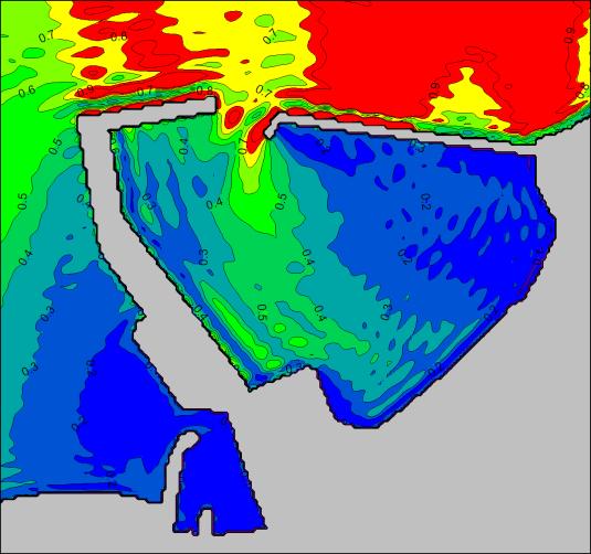
97 Results Presentation and Analysis In order to create 2D maps (and animations) of wave disturbance results in the Grid Plot tool, please drag and drop the file MzPlot.Wavedisturbance.plc (located in the folder.\kirkwall_marina\model_setup_1 ) into the MIKE Zero shell. After loading the data file, you will see an image as shown in Figure 5.8. The setup includes a map for the entire model area and a map for the Kirkwall Marina. Click on View (in the menu bar) Export Graphics (or shortcut Ctrl B) Save to Bitmap and you create e.g. a PNG-file as shown in Figure 5.9. The wave reflection is easy to recognise inside as well as outside of the marina basin. Please also check the statistical results for stationarity, i.e. that the wave disturbance coefficient (or wave height) at a given location is almost constant in time at the end of the simulation (25 minutes). One way to check this is by extracting the results at selected points using the MIKE Zero Toolbox Extraction tool. Load MIKE Zero Ctrl N MIKE Zero Toolbox Extraction Time Series from 2D files, see Figure On the introduction page (Figure 5.11) you may add a setup name (here e.g. Wave Disturbance 1 ). On the next two pages you add the name and location of the input data file and specify the required time period. Figure 5.8 Statistical results 2D visualisation using MIKE Zero Plot Composer Grid Plot. Wave disturbance coefficients in the Bay of Kirkwall. Wave conditions: H m0= 1.5 m, T p= 5.5 s, MWD= 360 N, WL= m, JONSWAP frequency spectrum and cos 8 -directional distribution 93

98 MIKE 21 Figure 5.9 Wave disturbance coefficients in the Bay of Kirkwall (upper panel) and in the Kirkwall Marina (lower panel). Wave conditions: H m0= 1.5 m, T p= 5.5 s, MWD= 360 N, WL= m, JONSWAP frequency spectrum and cos 8 -directional distribution 94 Boussinesq Wave Module - DHI

99 Results Presentation and Analysis Figure 5.10 Extraction of time series from a map (2D data file) using MIKE Zero Toolbox Extraction tool Figure 5.11 Introduction page on MIKE Zero Toolbox Extraction tool wizard 95

100 MIKE 21 Figure 5.12 Specify input data file Figure 5.13 Select time period 96 Boussinesq Wave Module - DHI

101 Results Presentation and Analysis Next, you should select the items to extract (Figure 5.14) and in Figure 5.15, the number of points to extraction and the grid coordinate should be specified. Here, we will use the same points as depicted in Figure 5.6. On the next wizard page, you should specify the output file name and location (Figure 5.16). The last page (Figure 5.17) gives you the status of the tool setup. Figure 5.14 Select items to extract Figure 5.15 Specify number of points to extract and location 97

102 MIKE 21 Figure 5.16 Specify output data Figure 5.17 Status page Now, click on the execution button. After few seconds, a time series plot pops up, see Figure 5.18 indicating a successful extraction. The time series show that the significant wave height at this position P(1200 m, 1800 m) is not yet stable due to strong reflection from the main breakwater at Hatston Ferry Terminal, see Figure 5.9. Click on the OK button and hereafter the Finish button. If you plan to extract data from other simulations later on, please save the extraction specification into a file, e.g. Extraction.MZT in the folder./kirkwall_marina\model_setup_1. 98 Boussinesq Wave Module - DHI

103 Results Presentation and Analysis The extracted data can be visualised in the MIKE Zero Time Series Editor (simply drag and drop the generated file ts_wave_disturbance1.dfs0 into a MIKE Zero shell) or use the Plot Composer (see previous section). Figure 5.19 shows a plot of the generated time series. From this figure it appears that 25 minutes' simulation time is sufficient to obtain an almost stationary situation. Figure 5.18 After execution 99

104 MIKE 21 Figure 5.19 Time series of wave disturbance coefficient at three different locations (see Figure 5.6) An alternative and perhaps more efficient procedure to check the stationarity is to use the Data Viewer tool available in MIKE Zero. Use the Open with feature as illustrated in Figure After the loading is completed, please click on the Position of time series button ( ) and specify the selected points using either the tabular menu or by clicking on the map, see Figure Figure 5.20 Data Viewer in MIKE Zero 100 Boussinesq Wave Module - DHI

105 Results Presentation and Analysis Figure 5.21 Specify location of time series (in distance from model origo in metres Figure 5.22 Image of wave disturbance map in MIKE Zero Data Viewer and location of extracted time series (t1, t2 and t3) 101

106 MIKE 21 Here, we use the same locations as used in the Figure The positions are automatically depicted on the map, see Figure Next you click on the OK button and a time series plot (as shown in Figure 5.23) appears on the screen. The extracted time series data may now be stored (dfs0 file). Figure 5.23 Time series of wave disturbance coefficient at three different locations extracted interactively using the Data Viewer tool 5.3 Further Analysis Quite often further analysis of the model results is required, e.g. analysis of potential long wave agitation and risk of seiching and harbour resonance. The WS Wave Analysis Tools (WSWAT) package integrated in MIKE Zero 12 includes a number of advanced modules for such and many other analyses, see Figure The intention of this section is to illustrate the potential and the application of this analysis package. Therefore, a detailed walk-through is not included. 12 The WS Wave Analysis Tools package requires a separate licence 102 Boussinesq Wave Module - DHI

107 Results Presentation and Analysis Figure 5.24 WS Wave Analysis Tools (WSWAT) is included in MIKE Zero For assessment of potential long waves inside the Kirkwall Marina, we will perform a spectral analysis of the time series shown in Figure 5.6. For that purpose, the WS Linear Spectral Analysis module is applied. The estimated frequency spectra at the three locations are presented in Figure As seen from figure, most of the wave energy inside the port is on the frequency corresponding to the peak period of the offshore waves, i.e. 5.5s (or frequency 0.18 Hz). However, a small portion of wave energy also occurs in the low frequency band. The low frequency peak occurs at a wave period corresponding to approximately 60 s, which is in good agreement with the fundamental natural period of harbour, see below. The low frequency waves can be analysed further using the WS Digital Filtering Analysis Tool module. As this module support 2D data (dfs2), it is easy to make a band pass filtering of the surface elevation in order to separate the long waves. Here, we will focus on waves within the period interval s (corresponding frequency band is Hz). As a higher temporal resolution output is required, we re-run the MIKE 21 BW simulation and store the data every 2 seconds and every 6 metres. This returns an approximately 1.2 GB data file including the simulated surface elevation. Next, the file is loaded into the WS Digital Filtering Analysis module and the analysis parameters are specified. 103

108 MIKE 21 Figure 5.25 Estimated frequency spectra (upper panel with linear ordinate and lower logarithmic) at three locations shown in Figure 5.6. The spectra are calculated by the WS Linear Spectral Analysis module The output is a band pass filtering dfs2 data file, which easily can be visualised and animated in e.g. Grid Plot. Figure 5.26 shows a snapshot of the results. The low frequency oscillation mode is clearly seen from such a map. Antinodes occur at the wave absorber and at the fully reflective western breakwater. This is even clearer, if we extract a line series from the generated data file 13 as sketched in Figure 5.26, which shows an envelope plot of the extracted surface elevation. The node and antinodes are clearly seen. A map of distribution of the long wave energy is shown in Figure This type of output can also be stored in the analysis tool. 13 MIKE Zero Toolbox Extraction Profile series from 2D files. 104 Boussinesq Wave Module - DHI

109 Results Presentation and Analysis Figure 5.26 Band pass (BP) filtered surface elevation (40-80s) calculated by the WS Digital Filtering Analysis module. The upper panel shows a map of instantaneous BP filtered surface elevation. The lower panel shows an envelope plot of the BP filtered surface elevation along the depicted line 105

110 MIKE 21 Figure 5.27 Map of normalised long wave energy inside the Kirkwall Marina Finally, the WS Directional Wave Analysis module 14 is an efficient tool for directional analysis of concurrent data of surface elevation and fluxes computed by MIKE 21 BW. The tool supports time series data (dfs0) and Grid series data (dfs2). Examples of output from this tool are shown in Figure 5.28 and Figure The first figure shows polar plot of the estimated directional wave spectra at two locations in the harbour. The second plot shows maps of estimated significant wave height and mean wave direction. Figure 5.28 Estimated directional wave spectra at the harbour entrance and at the wave absorber (locations in Figure 5.6). The spectra is calculated by the WS Directional Wave Analysis module 14 The module is based on the maximum entropy method (MEM) and assumes weakly reflective waves. 106 Boussinesq Wave Module - DHI

111 Results Presentation and Analysis Figure 5.29 Calculated mean wave direction on top of a map showing the significant wave height. The results are calculated by the WS Directional Wave Analysis module 107

112 MIKE Boussinesq Wave Module - DHI

113 Comparison between MIKE 21 BW and Physical Model Test Data 6 Comparison between MIKE 21 BW and Physical Model Test Data 6.1 Model Setup As mentioned in Section 1.1, DHI has tested the existing marina layout (May 2005) in a non-distorted physical model, see Figure 6.1. All model tests were carried out with irregular long-crested (uni-directional) waves generated on basis of a standard JONSWAP spectrum. For a proper comparison between numerical and physical model results, a MIKE 21 BW simulation with unidirectional waves has to be setup. First, you have to generate the internal wave generation data. Please load the file Input_setup1.21t (in folder.\\kirkwall_marina\model_setup_1 ) into MIKE Zero. Click on Waves Random Wave Generation and select the setup Hm0= 1.5m, Tp=5.5s, WD=360deg. N, WL= CDm, Uni. Waves. Next, you click on the run button, see Figure 6.2. Figure 6.1 Physical model of the Kirkwall Marina 109

114 MIKE 21 Figure 6.2 Creation of internal wave generation data (unidirectional waves) Then you load the prepared model setup file Model_setup1_Unidir.bw (in folder.\\kirkwall_marina\model_setup_1 ) and execute the simulation. The setup is identical to the setup that we have used in the previous sections, except that the incident waves are now unidirectional. In addition, we have changed the names of the output files. 6.2 Model Results Figure 6.3 shows an image of the instantaneous surface elevation at an early stage of the simulation. Figure 6.4 shows images of the wave disturbance coefficient for the simulation with unidirectional and directional incident waves, respectively. The percentage difference between these two maps is presented in Figure 6.5. This figure shows that the wave disturbance inside the marina in many places is higher for unidirectional waves. 110 Boussinesq Wave Module - DHI

115 Comparison between MIKE 21 BW and Physical Model Test Data Figure 6.3 3D visualisation of instantaneous surface elevation in the Bay of Kirkwall (unidirectional incident waves) 111

116 MIKE 21 Unidirectional waves Directional waves Figure 6.4 Wave disturbance coefficients in Kirkwall Marina. Wave conditions: H m0= 1.5 m, T p= 5.5 s, MWD= 360 N, WL= m, JONSWAP frequency spectrum and unidirectional (upper panel)/cos 8 -directional distribution (lower panel). 112 Boussinesq Wave Module - DHI

117 Comparison between MIKE 21 BW and Physical Model Test Data Figure 6.5 Percentage difference between wave disturbance for unidirectional and directional incident waves 6.3 Comparison The positions of the wave gauges used in the physical model are shown in Figure 6.6, and the corresponding positions in the numerical model are depicted in Figure 6.7. In order to compare the results from the two models, the significant wave height is scaled with the wave height at wave gauge 14, located offshore. The comparison is presented in Figure 6.8. By comparing the results from the physical modelling with the results of the numerical simulation, it is concluded that the two models are generally in excellent agreement - both with respect to magnitudes and the spatial variation of the wave disturbance inside the Kirkwall Marina. 113

118 MIKE 21 Figure 6.6 Positions of wave gauges in the physical model Figure 6.7 Positions of wave gauges in the numerical model. The wave height is normalised with the wave height at wave gauge Boussinesq Wave Module - DHI

119 Comparison between MIKE 21 BW and Physical Model Test Data Figure 6.8 Comparison between measured (physical model) and simulated (MIKE 21 BW) wave disturbance coefficients. Wave gauge locations are shown in Figure 6.7 At wave gauge 5, the physical model results in approximately 40% higher waves, which most likely is caused by wave overtopping the eastern breakwater. Wave overtopping is not included in MIKE 21 BW. Please also note that the incident significant wave height was 1.9 m in the physical model and 1.5 m in the Boussinesq model. All other wave parameters are identical. At wave gauges 2 and 3, the numerical model gives somewhat higher waves compared to the physical model. As the wave gauges are located in a highly reflected wave field, even minor differences between the wave gauge positions may have a large impact on the results. This is probably also the case at wave gauge 13, where the physical model predicts approximately 25% higher waves compared to numerical model results. Neglecting these three wave gauges (WGs 2, 3 and 5), the average difference between the physical and the numerical model results is less than 10%. 115