DECEMBER 2012 URBANMOBILITY REPORT POWERED BY REGION UNIVERSITY TRANSPORTATION CENTER

Transcription

1 URBANMOBILITY REPORT DECEMBER POWERED BY REGION UNIVERSITY TRANSPORTATION CENTER

2 TTI s 2012 URBAN MOBILITY REPORT Powered by INRIX Traffic Data David Schrank Associate Research Scientist Bill Eisele Senior Research Engineer And Tim Lomax Senior Research Engineer Texas A&M Transportation Institute The Texas A&M University System December 2012

3 DISCLAIMER The contents of this report reflect the views of the authors, who are responsible for the facts and the accuracy of the information presented herein. This document is disseminated under the sponsorship of the U.S. Department of Transportation University Transportation Centers Program in the interest of information exchange. The U.S. Government assumes no liability for the contents or use thereof. Acknowledgements Shawn Turner, David Ellis, Greg Larson, Tyler Fossett, and Phil Lasley Concept and Methodology Development Bonnie Duke and Michelle Young Report Preparation Lauren Geng and Jian Shen GIS Assistance Tobey Lindsey Web Page Creation and Maintenance Richard Cole, Rick Davenport, Bernie Fette and Michelle Hoelscher Media Relations John Henry Cover Artwork Dolores Hott and Nancy Pippin Printing and Distribution Rick Schuman, Ken Kranseler, and Jim Bak of INRIX Technical Support and Media Relations Paul Meier and Scott Williams of the Energy Institute at the University of Wisconsin-Madison CO 2 Methodology Review Support for this research was provided in part by a grant from the U.S. Department of Transportation University Transportation Centers Program to the Southwest Region University Transportation Center (SWUTC). TTI s 2012 Urban Mobility Report Powered by INRIX Traffic Data

4 Table of Contents Page 2012 Urban Mobility Report... 1 Turning Congestion Data Into Knowledge... 2 One Page of Congestion Problems... 5 More Detail About Congestion Problems... 6 The Trouble With Planning Your Trip... 8 The Future of Congestion Unreliable Travel Times Air Quality Impacts of Congestion Freight Congestion and Commodity Value Possible Solutions The Next Generation of Freight Measures Congestion Relief An Overview of the Strategies Congestion Solutions The Effects Benefits of Public Transportation Service Better Traffic Flow More Capacity Total Peak Period Travel Time Calculation Methods Using the Best Congestion Data & Analysis Methodologies Future Changes Concluding Thoughts Solutions and Performance Measurement References Sponsored by: Southwest Region University Transportation Center Texas A&M University National Center for Freight and Infrastructure Research and Education (CFIRE) University of Wisconsin Texas A&M Transportation Institute TTI s 2012 Urban Mobility Report Powered by INRIX Traffic Data iii

5

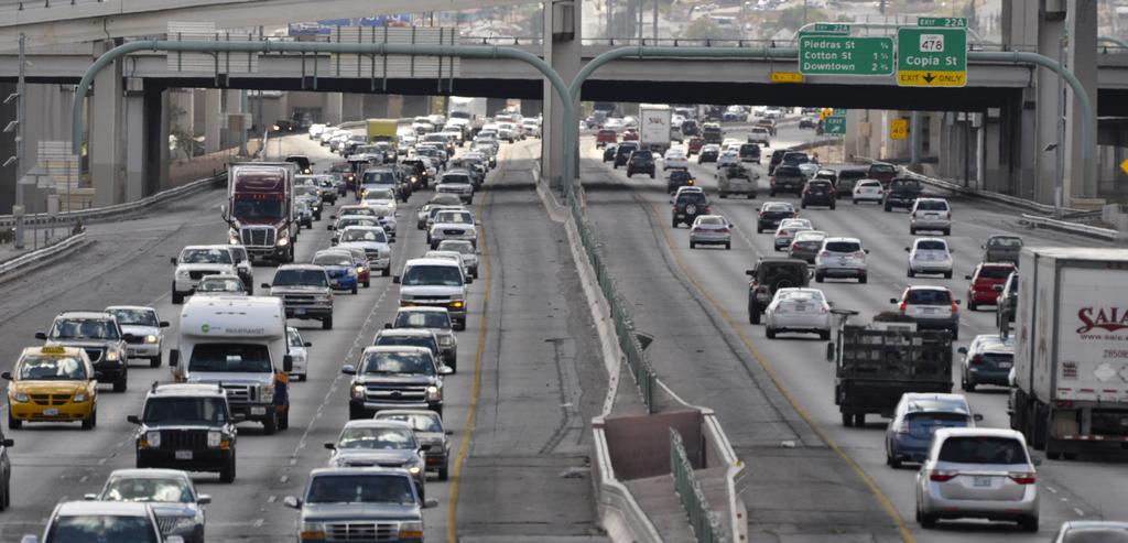
6 2012 Urban Mobility Report Congestion levels in large and small urban areas were buffeted by several trends in Some caused congestion increases and others decreased stop-and-go traffic. For the complete report and congestion data on your city, see: The 2011 data are consistent with one past trend, congestion will not go away by itself action is needed! (see Exhibit 1) The problem is very large. In 2011, congestion caused urban Americans to travel 5.5 billion hours more and to purchase an extra 2.9 billion gallons of fuel for a congestion cost of $121 billion. Second, in order to arrive on time for important trips, travelers had to allow for 60 minutes to make a trip that takes 20 minutes in light traffic. Third, while congestion is below its peak in 2005, there is only a short-term cause for celebration. Prior to the economy slowing, just 5 years ago, congestion levels were much higher than a decade ago; these conditions will return as the economy improves. The data show that congestion solutions are not being pursued aggressively enough. The most effective congestion reduction strategy, however, is one where agency actions are complemented by efforts of businesses, manufacturers, commuters and travelers. There is no rigid prescription for the best way each region must identify the projects, programs and policies that achieve goals, solve problems and capitalize on opportunities. Exhibit 1. Major Findings of the 2012 Urban Mobility Report (498 U.S. Urban Areas) (Note: See page 2 for description of changes since the 2011 Report) Measures of Individual Congestion Yearly delay per auto commuter (hours) Travel Time Index Planning Time Index (Freeway only) Wasted" fuel per auto commuter (gallons) CO 2 per auto commuter during congestion (lbs) Congestion cost per auto commuter (2011 dollars) $342 $795 $924 $810 $818 The Nation s Congestion Problem Travel delay (billion hours) Wasted fuel (billion gallons) CO 2 produced during congestion (billions of lbs) Truck congestion cost (billions of 2011 dollars) Congestion cost (billions of 2011 dollars) $24 $94 $128 $120 $121 The Effect of Some Solutions Yearly travel delay saved by: Operational treatments (million hours) Public transportation (million hours) Yearly congestion costs saved by: Operational treatments (billions of 2011$) $0.2 $3.6 $7.3 $8.3 $8.5 Public transportation (billions of 2011$) $8.0 $14.0 $18.5 $20.2 $20.8 Yearly delay per auto commuter The extra time spent traveling at congested speeds rather than free-flow speeds by private vehicle drivers and passengers who typically travel in the peak periods. Travel Time Index (TTI) The ratio of travel time in the peak period to travel time at free-flow conditions. A Travel Time Index of 1.30 indicates a 20-minute free-flow trip takes 26 minutes in the peak period. Commuter Stress Index The ratio of travel time for the peak direction to travel time at free-flow conditions. A TTI calculation for only the most congested direction in both peak periods. Planning Time Index (PTI) The ratio of travel time on the worst day of the month to travel time at free-flow conditions. A Planning Time Index of 1.80 indicates a traveler should plan for 36 minutes for a trip that takes 20 minutes in free-flow conditions (20 minutes x 1.80 = 36 minutes). The Planning Time Index is only computed for freeways only; it does not include arterials. Wasted fuel Extra fuel consumed during congested travel. CO 2 per auto commuter during congestion The extra CO 2 emitted at congested speeds rather than free-flow speed by private vehicle drivers and passenger who typically travel in the peak periods. Congestion cost The yearly value of delay time and wasted fuel. TTI s 2012 Urban Mobility Report Powered by INRIX Traffic Data $ $27

7 Turning Congestion Data Into Knowledge (And the New Data Providing a More Accurate View) The 2012 Urban Mobility Report is the 3 rd prepared in partnership with INRIX (1), a leading private sector provider of travel time information for travelers and shippers. The data behind the 2012 Urban Mobility Report are hundreds of speed data points on almost every mile of major road in urban America for almost every 15-minute period of the average day. For the congestion analyst, this means 600 million speeds on 875,000 miles across the U.S. an awesome amount of information. For the policy analyst and transportation planner, this means congestion problems can be described in detail and solutions can be targeted with much greater specificity and accuracy. Exhibit 2 shows historical national congestion trend measures. Key aspects of the 2012 UMR are summarized below. Speeds collected every 15-minutes from a variety of sources every day of the year on most major roads are used in the study. For more information about INRIX, go to The data for all 24 hours makes it possible to track congestion problems for the midday, overnight and weekend time periods. A measure of the variation in travel time from day-to-day is introduced. The Planning Time Index (PTI) is based on the idea that travelers would want to be on-time for an important trip 19 out of 20 times; so one would be late only one day per month (on-time for 19 out of 20 work days each month). A PTI value of 3.00 indicates that a traveler should allow 60 minutes to make an important trip that takes 20 minutes in uncongested traffic. In essence, the 19 th worst commute is affected by crashes, weather, special events, and other causes of unreliable travel and can be improved by a range of transportation improvement strategies. Truck freight congestion is explored in more detail thanks to research funding from the National Center for Freight and Infrastructure Research and Education (CFIRE) at the University of Wisconsin ( Additional carbon dioxide (CO 2 ) greenhouse gas emissions due to congestion are included for the first time thanks to research funding from CFIRE and collaboration with researchers at the Energy Institute at the University of Wisconsin-Madison. The procedure is based on the Environmental Protection Agency s Motor Vehicle Emission Simulator (MOVES) modeling procedure. Wasted fuel is estimated using the additional carbon dioxide greenhouse gas emissions due to congestion for each urban area. For the first time, this method allows for consideration of urban area climate in emissions and fuel consumption calculations. More information on these new measures and data can be found at: TTI s 2012 Urban Mobility Report Powered by INRIX Traffic Data 2

8 3 Exhibit 2. National Congestion Measures, 1982 to 2011 Hours Saved (million hours) Gallons Saved (million gallons) Dollars Saved (billions of 2011$) Travel Delay per Total Delay Fuel Wasted Total Cost Operational Treatments Operational Treatments Operational Treatments Year Time Index Commuter (hours) (billion hours) (billion gallons) (2011$ billion) & HOV Lanes Public Transp & HOV Lanes Public Transp & HOV Lanes Public Transp Note: For more congestion information see Tables 1 to 10 and

9

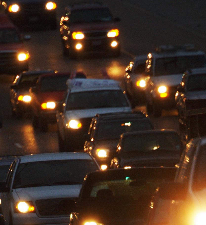
10 One Page of Congestion Problems In many regions, traffic jams can occur at any daylight hour, many nighttime hours and on weekends. The problems that travelers and shippers face include extra travel time, unreliable travel time and a system that is vulnerable to a variety of irregular congestion-producing occurrences. Some key descriptions are listed below. See data for your city at Congestion costs are increasing. The congestion invoice for the cost of extra time and fuel in 498 urban areas was (all values in constant 2011 dollars): In 2011 $121 billion In 2000 $94 billion In 1982 $24 billion Congestion wastes a massive amount of time, fuel and money. In 2011: 5.5 billion hours of extra time (equivalent to the time businesses and individuals spend a year filing their taxes). 2.9 billion gallons of wasted fuel (enough to fill four New Orleans Superdomes). $121 billion of delay and fuel cost (the negative effect of uncertain or longer delivery times, missed meetings, business relocations and other congestion-related effects are not included) ($121 billion is equivalent to the lost productivity and direct medical expenses of 12 average flu seasons). 56 billion pounds of additional carbon dioxide (CO 2 ) greenhouse gas released into the atmosphere during urban congested conditions (equivalent to the liftoff weight of over 12,400 Space Shuttles with all fuel tanks full). 22% ($27 billion) of the delay cost was the effect of congestion on truck operations; this does not include any value for the goods being transported in the trucks. The cost to the average commuter was $818 in 2011 compared to an inflation-adjusted $342 in Congestion affects people who travel during the peak period. The average commuter: Spent an extra 38 hours traveling in 2011, up from 16 hours in Wasted 19 gallons of fuel in 2011 a week s worth of fuel for the average U.S. driver up from 8 gallons in In areas with over three million persons, commuters experienced an average of 52 hours of delay in Suffered 6 hours of congested road conditions on the average weekday in areas over 3 million population. Fridays are the worst days to travel. The combination of work, school, leisure and other trips mean that urban residents earn their weekend after suffering over 20 percent more delay hours than on Mondays. And if all that isn t bad enough, folks making important trips had to plan for approximately three times as much travel time as in light traffic conditions in order to account for the effects of unexpected crashes, bad weather, special events and other irregular congestion causes. Congestion is also a problem at other hours. Approximately 37 percent of total delay occurs in the midday and overnight (outside of the peak hours) times of day when travelers and shippers expect free-flow travel. Many manufacturing processes depend on a free-flow trip for efficient production and congested networks interfere with those operations. TTI s 2012 Urban Mobility Report Powered by INRIX Traffic Data 5

11 More Detail About Congestion Problems Congestion, by every measure, has increased substantially over the 30 years covered in this report. And congestion is recovering from the improvements seen during the economic recession; many regions have seen congestion get worse as the economy gets better. As in past regional recessions (see California s dot com bubble in the early 2000s) when the economy recovers, so does traffic congestion and when unemployment lines shrank, lines of bumper-tobumper traffic grew. Recent trends show traffic congestion for commuters is relatively stable over the last few years after a decline at the start of the economic recession. The total congestion cost has risen as more commuters and freight shippers use the system. This trend is similar to past regional recessions and fuel price increases. Travel patterns change initially, and then travelers return to previous habits and congestion increases return to their previous pattern. There is still time to use this reset in the congestion trend, as well as the low prices for construction, to promote congestion reduction programs, policies and projects. But time is probably running out on the lower-cost construction period. Congestion is worse in areas of every size it is not just a big city problem. The growing delays also hit residents of smaller cities (Exhibit 3). Big towns and small cities alike cannot implement enough projects, programs and policies to meet the demands of growing population and jobs. Major projects, programs and funding efforts take 10 to 15 years to develop. Exhibit 3. Congestion Growth Trend Small = less than 500,000 Medium = 500,000 to 1 million Large = 1 million to 3 million Very Large = more than 3 million Think of what else could be done with the 38 hours of extra time suffered by the average urban auto commuter in 2011: Almost 5 vacation days Equivalent to over one and a half times what Americans spend online shopping every year. Equivalent to the amount of time Americans spend over the winter holidays gift shopping, attending holiday parties and traveling to holiday parties. TTI s 2012 Urban Mobility Report Powered by INRIX Traffic Data 6

12 Congestion builds through the week from Monday to Friday. The two weekend days have less delay than any weekday (Exhibit 4). Congestion is worse in the evening, but it can be a problem all day (Exhibit 5). Midday hours comprise a significant share of the congestion problem. Exhibit 4. Percent of Delay for Each Day Exhibit 5. Percent of Delay by Time of Day Day of Week Hour of Day Streets have more delay than freeways (Exhibit 6). Exhibit 6. Percent of Delay for Road Types The surprising congestion levels have logical explanations in some regions. The urban area congestion level rankings shown in Tables 1 through 10 (pgs ) may surprise some readers. The areas listed below are examples of the reasons for higher than expected congestion levels. Work zones Baton Rouge. Construction, even when it occurs in the off-peak, can increase traffic congestion. Smaller urban areas with a major interstate highway Austin, Bridgeport, Salem. High volume highways running through smaller urban areas generate more traffic congestion than the local economy causes by itself. Tourism Orlando, Las Vegas. The traffic congestion measures in these areas are divided by the local population numbers causing the per-commuter values to be higher than normal. Geographic constraints Honolulu, Pittsburgh, Seattle. Water features, hills and other geographic elements cause more traffic congestion than regions with several alternative routes. TTI s 2012 Urban Mobility Report Powered by INRIX Traffic Data 7

13 The Trouble With Planning Your Trip We ve all made urgent trips catching an airplane, getting to a medical appointment, or picking up a child at daycare on time. We know we need to leave a little early to make sure we are not late for these important trips, and we understand that these trips will take longer during the rush hour. We are conditioned to add some extra time to these trips to make sure we make it, just in case there is an event that causes some unexpected congestion. The need to add extra times isn t just a rush hour consideration. Trips during the off-peak can also take longer than expected. If we have to catch an airplane at 1 p.m. in the afternoon, we might still be inclined to add a little extra time, and the data indicate that our intuition is correct. Exhibit 7 illustrates this idea. Say your typical trip takes 20 minutes when there are few other cars on the road. That is represented by the green bar across the morning, midday, and evening. Now imagine that your trip takes just a little longer, on average, whether that trip is in the morning, midday, or evening. This average trip time is shown in the solid yellow bar in Exhibit 7. Now consider that you have a very important trip to make during any of these time periods there is additional planning time you must provide to ensure you make that trip ontime. And, as shown in Exhibit 7 (red bar), it isn t just a rush hour problem it can happen any time of the day. The analysis shown in the report (Table 3) indicates that folks making important trips on freeways during the peak periods had to plan for approximately three (3) times as much travel time as in light traffic conditions in order to account for the effects of unexpected crashes, bad weather, and other irregular congestion causes. Page 10 describes trip reliability in more detail. Exhibit 7. Extra Time to Make Important Trips. TTI s 2012 Urban Mobility Report Powered by INRIX Traffic Data 8

14 Travelers and shippers must plan around congestion more often. In all 498 urban areas, the worst congestion levels affected only 1 in 9 trips in 1982, but almost 1 in 4 trips in 2011 (Exhibit 8). The most congested sections of road account for 78% of peak period delays, with only 21% of the travel (Exhibit 8). Delay has grown about five times larger overall since 1982 (Exhibit 2). Exhibit 8. Peak Period Congestion and Congested Travel in 2011 Vehicle travel in congestion ranges Travel delay in congestion ranges While trucks only account for about 7 percent of the miles traveled in urban areas, they are almost 23 percent of the urban congestion invoice. In addition, the cost in Exhibit 9 only includes the cost to operate the truck in heavy traffic; the extra cost of the commodities is not included. Exhibit Congestion Cost for Urban Passenger and Freight Vehicles Travel by Vehicle Type Congestion Cost by Vehicle Type TTI s 2012 Urban Mobility Report Powered by INRIX Traffic Data 9

15

16 The Future of Congestion A few years ago, a congestion forecast of more would not be unusual. With the economic recession reducing congestion over the last few years, such predictions are more difficult. The 2012 Urban Mobility Report, however, uses expected population growth figures to provide some estimates to illustrate the near-future congestion problem. Congestion is the result of an imbalance between travel demand and the supply of transportation capacity; so if the number of people or jobs goes up, or the miles or trips that those people make increases, the road and transit systems also need to expand. As this report demonstrates, however, this is an infrequent occurrence, and travelers are paying the price for this inadequate response. Population and employment growth two primary factors in rush hour travel demand are projected to grow slightly slower from 2012 to 2020 than in the previous ten years. The combined role of the government and private sector will yield approximately the same rate of transportation system expansion (both roadway and public transportation). The analysis assumes that policies and funding levels will remain about the same. The growth in usage of any of the alternatives (biking, walking, work or shop at home) will continue at the same rate. Decisions as to the priorities and level of effort in solving transportation problems will continue as in the recent past. The period before the economic recession was used as the indicator of the effect of growth. These years had generally steady economic growth in most U.S. urban regions; these years are assumed to be a good indicator of the future level of investment in solutions and the resulting increase in congestion. If this status quo benchmark is applied to the next five to ten years, a rough estimate of future congestion can be developed. The congestion estimate for any single region will be affected by the funding, project selections and operational strategies; the simplified estimation procedure used in this report will not capture these variations. Combining all the regions into one value for each population group, however, may result in a balance between estimates that are too high and those that are too low. The national congestion cost will grow from $121 billion to $199 billion in 2020 (in 2011 dollars). Delay will grow to 8.4 billion hours in Wasted fuel will increase to 4.5 billion gallons in The average commuter will see their cost grow to $1,010 in 2020 (in 2011 dollars). They will waste 45 hours and 25 gallons in If the price of gasoline grows to $5 per gallon, the congestion-related fuel cost would grow from about $10 billion in 2011 to approximately $22 billion in 2020 (in 2011 dollars). TTI s 2012 Urban Mobility Report Powered by INRIX Traffic Data 11

17 Unreliable Travel Times The Annoying Issue of not Knowing How Long Your Trip Will Take Trips take longer in rush hour, we all get that. But when you really need to be somewhere at a specific time - whether it s a family dinner, a meeting, an airplane departure or a health care appointment - you have to plan for the possibility of an even longer trip. As bad as traffic jams are, it s even more frustrating that you can t depend on how bad the traffic will be. For the first time, the Urban Mobility Report includes a measure of this frustrating extra extra travel time the amount of time you have to allow above the regular travel time. The INRIX dataset catalogs many trips taken on each road section; these have been analyzed to identify the longest trip times and present them in a measure similar to the Travel Time Index. The Planning Time Index (PTI) identifies the extra time that should be allowed to arrive on-time for a trip 19 times out of 20. Statistically, this is the 95 th percentile and it speaks to the effects of a variety of events that make travel time unpredictable. Exhibit 10 shows how traffic conditions have historically been communicated with averages. As shown in Exhibit 10, we all know that traffic isn t average everyday, it varies greatly. When your travel time is very high due to a large crash, special event, bad weather, or unexpected construction, your trip can take much longer. This variability in traffic is what the PTI helps you understand. If the PTI for your trip is 3.00, that tells you to plan 60 minutes for a trip that takes 20 minutes when there are few other cars on the road (20 minutes x 3.00 = 60 minutes) to ensure you are on-time for a trip 19 out of 20 times. Here s another way to think about it suppose your boss tells you that it is ok to be late for work only 1 day out of the 20 workdays per month, the PTI would help you understand how much time to allow to satisfy your boss requirement. In addition to PTI, Table 3 (pgs ) also includes a reliability performance measure designed for transportation agency evaluation. PTI 80 shows the worst trip of the week the extra time to ensure timely arrival for 4 out of 5 trips. The worst trip of the week is frequently caused by a crash; rapid removal of these can improve PTI 80. Bad weather that causes several of the worst travel times must be planned for, but it s difficult to grade an agency on weather conditions. The methodology in the appendix provides further discussion and explanation of PTI and PTI 80. Exhibit 10. Your Trip Can Vary Greatly Source: Federal Highway Administration (2) TTI s 2012 Urban Mobility Report Powered by INRIX Traffic Data 12

18 Air Quality Impacts of Congestion According to the Environmental Protection Agency (EPA), transportation is the second largest emitting sector of carbon dioxide (CO 2 ) greenhouse gases behind electricity generation (3). There is increasing interest in the impact of transportation on air quality. For the first time, the 2012 Urban Mobility Report includes measures of the additional CO 2 emissions as a result of congestion. With funding from the Center for Freight and Infrastructure Research and Education (CFIRE) at the University of Wisconsin-Madison, TTI researchers teamed with researchers at the Energy Institute at the University of Wisconsin to develop a methodology to include CO 2 emissions in the UMR. The methodology uses data from three primary sources, 1) HPMS, 2) INRIX traffic speeds, and 3) the EPA s MObile Vehicle Emission Simulator (MOVES) model. MOVES provides emissions estimates for mobile sources. Researchers used MOVES extensively to develop CO 2 emission rates, which were used to calculate CO 2 emissions and subsequently wasted fuel estimates. More details regarding the methodology are shown in the appendix. Table 4 (pgs ) shows additional CO 2 production due to congestion by urban area size. Additional CO 2 production due to congestion in pounds per auto commuter and in total pounds for each urban area is shown. The 498 urban area total CO 2 produced by congestion is 56 billion pounds (equivalent to the takeoff weight of 12,400 space shuttles at liftoff with full fuel tanks). Note that this is only the additional CO 2 production due to congestion it does not include CO 2 production from auto commuters traveling when roadways are uncongested. A number of assumptions are in the model based upon available national-level data as inputs. These assumptions allow for a relatively simple and replicable method for 498 urban areas. More detailed and localized inputs should be used where available to improve local estimates of CO 2 production. Estimation of the additional CO 2 emissions due to congestion provides another important element to characterize the urban congestion problem. It provides useful information for decision-making and policy makers, and it points to the importance of implementing transportation improvements to mitigate congestion. Researchers plan to incorporate other air quality pollutants into future editions of the UMR. TTI s 2012 Urban Mobility Report Powered by INRIX Traffic Data 13

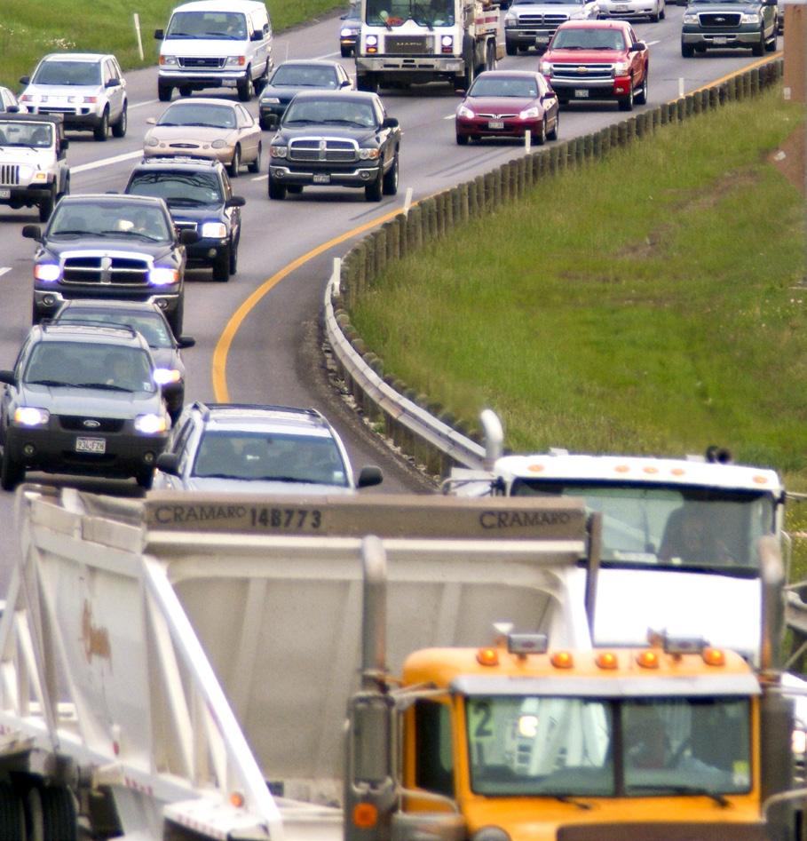
19 Freight Congestion and Commodity Value Trucks carry goods to suppliers, manufacturers and markets. They travel long and short distances in peak periods, middle of the day and overnight. Many of the trips conflict with commute trips, but many are also to warehouses, ports, industrial plants and other locations that are not on traditional suburb to office routes. Trucks are a key element in the just-in-time (or lean) manufacturing process; these business models use efficient delivery timing of components to reduce the amount of inventory warehouse space. As a consequence, however, trucks become a mobile warehouse; and if their arrival times are missed, production lines can be stopped, at a cost of many times the value of the truck delay times. Congestion, then, affects truck productivity and delivery times and can also be caused by high volumes of trucks, just as with high car volumes. One difference between car and truck congestion costs is important; it is intuitive that some of the $27 billion in truck congestion costs in 2011was passed on to consumers in the form of higher prices. The congestion effects extend far beyond the region where the congestion occurs. With funding from the National Center for Freight and Infrastructure Research and Education (CFIRE) at the University of Wisconsin and data from USDOT s Freight Analysis Framework (4), a methodology was developed to estimate the value of commodities being shipped by truck to and through urban areas and in rural regions. The commodity values were matched with truck delay estimates to identify regions where high values of commodities move on congested roadway networks. Table 5 (pgs ) points to a correlation between commodity value and truck delay higher commodity values are associated with more people; more people are associated with more traffic congestion. Bigger cities consume more goods, which means a higher value of freight movement. While there are many cities with large differences in commodity and delay ranks, only 23 urban areas are ranked with commodity values much higher than their delay ranking. Table 5 also illustrates the role of long corridors with important roles in freight movement. Some of the smaller urban areas along major interstate highways along the east and west coast and through the central and Midwestern U.S., for example, have commodity value ranks much higher than their delay ranking. High commodity values and lower delay might sound advantageous lower congestion levels with higher commodity values means there is less chance of congestion getting in the way of freight movement. At the areawide level, this reading of the data would be correct, but in the real world the problem often exists at the road or even intersection level and solutions should be deployed in the same variety of ways. TTI s 2012 Urban Mobility Report Powered by INRIX Traffic Data 14

20 Possible Solutions Urban and rural corridors, ports, intermodal terminals, warehouse districts and manufacturing plants are all locations where truck congestion is a particular problem. Some of the solutions to these problems look like those deployed for person travel new roads and rail lines, new lanes on existing roads, lanes dedicated to trucks, additional lanes and docking facilities at warehouses and distribution centers. New capacity to handle freight movement might be an even larger need in coming years than passenger travel capacity. Goods are delivered to retail and commercial stores by trucks that are affected by congestion. But upstream of the store shelves, many manufacturing operations use just-in-time processes that rely on the ability of trucks to maintain a reliable schedule. Traffic congestion at any time of day causes potentially costly disruptions. The solutions might be implemented in a broad scale to address freight traffic growth or targeted to road sections that cause freight bottlenecks. Other strategies may consist of regulatory changes, operating practices or changes in the operating hours of freight facilities, delivery schedules or manufacturing plants. Addressing customs, immigration and security issues will reduce congestion at border ports-of-entry. These technology, operating and policy changes can be accomplished with attention to the needs of all stakeholders and can produce as much from the current systems and investments as possible. The Next Generation of Freight Measures The dataset used for Table 5 provides origin and destination information, but not routing paths. The 2012 Urban Mobility Report developed an estimate of the value of commodities in each urban area, but better estimates of value will be possible when new freight models are examined. Those can be matched with the detailed speed data from INRIX to investigate individual congested freight corridors and their value to the economy. TTI s 2012 Urban Mobility Report Powered by INRIX Traffic Data 15

21

22 Congestion Relief An Overview of the Strategies We recommend a balanced and diversified approach to reduce congestion one that focuses on more of everything. It is clear that our current investment levels have not kept pace with the problems. Population growth will require more systems, better operations and an increased number of travel alternatives. And most urban regions have big problems now more congestion, poorer pavement and bridge conditions and less public transportation service than they would like. There will be a different mix of solutions in metro regions, cities, neighborhoods, job centers and shopping areas. Some areas might be more amenable to construction solutions, other areas might use more travel options, productivity improvements, diversified land use patterns or redevelopment solutions. In all cases, the solutions need to work together to provide an interconnected network of transportation services. More information on the possible solutions, places they have been implemented, the effects estimated in this report and the methodology used to capture those benefits can be found on the website or on the following websites below. Get as much service as possible from what we have Many low-cost improvements have broad public support and can be rapidly deployed. These management programs require innovation, constant attention and adjustment, but they pay dividends in faster, safer and more reliable travel. Rapidly removing crashed vehicles, timing the traffic signals so that more vehicles see green lights, improving road and intersection designs, or adding a short section of roadway are relatively simple actions. Add capacity in critical corridors Handling greater freight or person travel on freeways, streets, rail lines, buses or intermodal facilities often requires more. Important corridors or growth regions can benefit from more road lanes, new streets and highways, new or expanded public transportation facilities, and larger bus and rail fleets. Change the usage patterns There are solutions that involve changes in the way employers and travelers conduct business to avoid traveling in the traditional rush hours. Flexible work hours, internet connections or phones allow employees to choose work schedules that meet family needs and the needs of their jobs. Provide choices This might involve different routes, travel modes or lanes that involve a toll for high-speed and reliable service a greater number of options that allow travelers and shippers to customize their travel plans. Diversify the development patterns These typically involve denser developments with a mix of jobs, shops and homes, so that more people can walk, bike or take transit to more, and closer, destinations. Sustaining the quality of life and gaining economic development without the typical increment of mobility decline in each of these sub-regions appears to be part, but not all, of the solution. Realistic expectations are also part of the solution. Large urban areas will be congested. Some locations near key activity centers in smaller urban areas will also be congested. But congestion does not have to be an all-day event. Identifying solutions and funding sources that meet a variety of community goals is challenging enough without attempting to eliminate congestion in all locations at all times. TTI s 2012 Urban Mobility Report Powered by INRIX Traffic Data 17

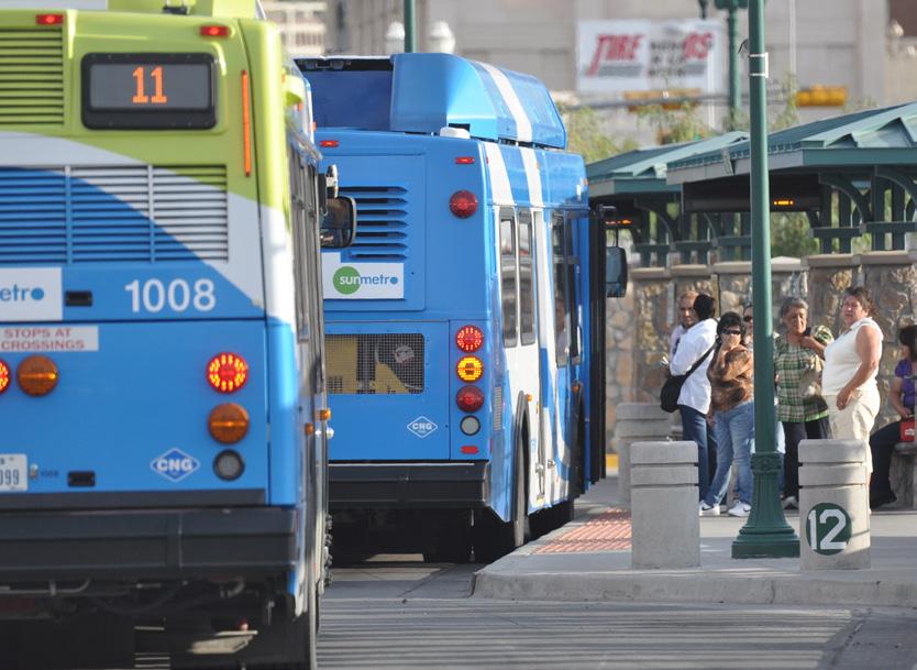
23 Congestion Solutions The Effects The 2012 Urban Mobility Report database includes the effect of several widely implemented congestion solutions. These strategies provide faster and more reliable travel and make the most of the roads and public transportation systems that have been built. These solutions use a combination of information, technology, design changes, operating practices and construction programs to create value for travelers and shippers. There is a double benefit to efficient operations-travelers benefit from better conditions and the public sees that their tax dollars are being used wisely. The estimates described in the next few pages are a reflection of the benefits from these types of roadway operating strategies and public transportation systems. Benefits of Public Transportation Service Regular-route public transportation service on buses and trains provides a significant amount of peak-period travel in the most congested corridors and urban areas in the U.S. If public transportation service had been discontinued and the riders traveled in private vehicles in 2011, the 498 urban areas would have suffered an additional 865 million hours of delay and consumed 450 million more gallons of fuel (Exhibit 11). The value of the additional travel delay and fuel that would have been consumed if there were no public transportation service would be an additional $20.8 billion, a 15% increase over current congestion costs in the 498 urban areas. There were approximately 56 billion passenger-miles of travel on public transportation systems in the 498 urban areas in 2011 (5). The benefits from public transportation vary by the amount of travel and the road congestion levels (Exhibit 11). More information on the effects for each urban area is included in Table 8 (pgs ). Population Group and Number of Areas Exhibit 11. Delay Increase in 2011 if Public Transportation Service Were Eliminated 498 Areas Average Annual Passenger-Miles of Travel (Million) Hours of Delay Saved (Million) Reduction Due to Public Transportation Percent of Gallons of Base Fuel Delay (Million) Dollars Saved ($ Million) Very Large (15) 43, ,415 Large (32) 6, ,939 Medium (33) 1, Small (21) Other (397) 4, ,060 National Urban Total 56, $20,784 Source: Reference (5) and Review by Texas A&M Transportation Institute TTI s 2012 Urban Mobility Report Powered by INRIX Traffic Data 18

24 Better Traffic Flow Improving transportation systems is about more than just adding road lanes, transit routes, sidewalks and bike lanes. It is also about operating those systems efficiently. Not only does congestion cause slow speeds, it also decreases the traffic volume that can use the roadway; stop-and-go roads only carry half to two-thirds of the vehicles as a smoothly flowing road. This is why simple volume-to-capacity measures are not good indicators; actual traffic volumes are low in stop-and-go conditions, so a volume/capacity measure says there is no congestion problem. Several types of improvements have been widely deployed to improve traffic flow on existing roadways. Five prominent types of operational treatments are estimated to relieve a total of 374 million hours of delay (7% of the total) with a value of $8.5 billion in 2011 (Exhibit 12). If the treatments were deployed on all major freeways and streets, the benefit would expand to almost 842 million hours of delay (15% of delay) and more than $19 billion would be saved. These are significant benefits, especially since these techniques can be enacted more quickly than significant roadway or public transportation system expansions can occur. The operational treatments, however, are not large enough to replace the need for those expansions. Exhibit 12. Operational Improvement Summary for All 498 Urban Areas Population Group and Number of Areas Reduction Due to Current Projects Hours of Delay Saved (Million) Gallons of Fuel Saved (Million) Dollars Saved ($ Million) Delay Reduction if In Place on All Roads (Million Hours) Very Large (15) , Large (33) , Medium (32) Small (21) Other (338) TOTAL $8, Note: This analysis uses nationally consistent data and relatively simple estimation procedures. Local or more detailed evaluations should be used where available. These estimates should be considered preliminary pending more extensive review and revision of information obtained from source databases (6,7). More information about the specific treatments and examples of regions and corridors where they have been implemented can be found at the website More Capacity Projects that provide more road lanes and more public transportation service are part of the congestion solution package in most growing urban regions. New streets and urban freeways will be needed to serve new developments, public transportation improvements are particularly important in congested corridors and to serve major activity centers, and toll highways and toll lanes are being used more frequently in urban corridors. Capacity expansions are also important additions for freeway-to-freeway interchanges and connections to ports, rail yards, intermodal terminals and other major activity centers for people and freight transportation. TTI s 2012 Urban Mobility Report Powered by INRIX Traffic Data 19

25 Additional roadways reduce the rate of congestion increase. This is clear from comparisons between 1982 and 2011 (Exhibit 13). Urban areas where capacity increases matched the demand increase saw congestion grow much more slowly than regions where capacity lagged behind demand growth. It is also clear, however, that if only areas were able to accomplish that rate, there must be a broader and larger set of solutions applied to the problem. Most of these regions (listed in Table 11 on page 97) were not in locations of high economic growth, suggesting their challenges were not as great as in regions with booming job markets. Exhibit 13. Road Growth and Mobility Level Source: Texas A&M Transportation Institute analysis, see and TTI s 2012 Urban Mobility Report Powered by INRIX Traffic Data 20

26 Total Peak Period Travel Time Another approach to measuring some aspects of congestion is the total time spent traveling during the peak periods. The measure can be used with other Urban Mobility Report statistics in a balanced transportation and land use pattern evaluation program. As with any measure, the analyst must understand the components of the measure and the implications of its use. In the Urban Mobility Report context where trends are important, values for cities of similar size and/or congestion levels can be used as comparisons. Year-to-year changes for an area can also be used to help an evaluation of long-term policies. The total peak period travel time measure is particularly well-suited for long-range scenario planning as it shows the effect of the combination of different transportation investments and land use arrangements. Some have used total travel time to suggest that it shows urban residents are making poor home and job location decisions or are not correctly evaluating their travel options. There are several factors that should be considered when examining values of total travel time. Travel delay The extra travel time due to congestion Type of road network The mix of high-speed freeways and slower streets Development patterns The physical arrangement of living, working, shopping, medical, school and other activities Home and job location Distance from home to work is a significant portion of commuting time Decisions and priorities It is clear that congestion is not the only important factor in the location and travel decisions made by families Individuals and families frequently trade one or two long daily commutes for other desirable features such as good schools, medical facilities, large homes or a myriad of other factors. Total peak period travel time (see Table 7 on pgs ) can provide additional explanatory power to a set of mobility performance measures. It provides some of the desirable aspects of accessibility measures, while at the same time being a travel time quantity that can be developed from actual travel speeds. Regions that are developed in a relatively compact urban form will also score well, which is why the measure may be particularly well-suited to public discussions about regional plans and how transportation and land use investments can support the attainment of community goals. Calculation Methods The 2012 Urban Mobility Report combines several datasets not traditionally used together to generate procedures and base data that produce a total travel time measure. Challenges clearly exist in creating a broader use for the data; additional development and refinement will address specific issues. For example, smaller cities ranking highly in Table 7 and larger cities ranking lower will require further clarification. This report measures total travel time in minutes of peakperiod road travel per auto commuter. Though capable of being a door-to-door metric in the future, values in Table 7 represent all travel only in automobiles and may appear to be less than average trip to work times reported by the US Census Bureau s American Community Survey (ACS) (8). The measure distinctly differs from the ACS by using real speed data instead of perceived travel times to generate a value for each urban area. The measure now includes delay and speeds (reference and congested) for local streets in its calculation. Other methodological refinements and a preliminary process for accounting for through trips have also been added. Researchers will continue to refine estimates of commuters, through trips, and local street travel as well as include other transportation modes. More information about the total peak period travel time measure can be found at: TTI s 2012 Urban Mobility Report Powered by INRIX Traffic Data 21

27 Using the Best Congestion Data & Analysis Methodologies The base data for the 2012 Urban Mobility Report come from INRIX, the U.S. Department of Transportation and the states (1,6). Several analytical processes are used to develop the final measures, but the biggest improvement in the last two decades is provided by INRIX data. The speed data covering most major roads in U.S. urban regions eliminates the difficult process of estimating speeds and dramatically improves the accuracy and level of understanding about the congestion problems facing US travelers. The methodology is described in a series of technical reports (9, 10, 11, 12) that are posted on the mobility report website: The INRIX traffic speeds are collected from a variety of sources and compiled in their National Average Speed (NAS) database. Agreements with fleet operators who have location devices on their vehicles feed time and location data points to INRIX. Individuals who have downloaded the INRIX application to their smart phones also contribute time/location data. The proprietary process filters inappropriate data (e.g., pedestrians walking next to a street) and compiles a dataset of average speeds for each road segment. TTI was provided a dataset of hourly average speeds for each link of major roadway covered in the NAS database for 2011 (approximately 875,000 directional miles in 2011). Hourly travel volume statistics were developed with a set of procedures developed from computer models and studies of real-world travel time and volume data. The congestion methodology uses daily traffic volume converted to average 15-minute volumes using a set of estimation curves developed from a national traffic count dataset (13). The 15-minute INRIX speeds were matched to the 15-minute volume data for each road section on the FHWA maps. An estimation procedure was also developed for the INRIX data that was not matched with an FHWA road section. The INRIX sections were ranked according to congestion level (using the Travel Time Index); those sections were matched with a similar list of most to least congested sections according to volume per lane (as developed from the FHWA data) (2). Delay was calculated by combining the lists of volume and speed. The effect of operational treatments and public transportation services were estimated using methods similar to previous Urban Mobility Reports. Future Changes There will be other changes in the report methodology over the next few years. There is more information available every year from freeways, streets and public transportation systems that provides more descriptive travel time and volume data. Congested corridor data and travel time reliability statistics are two examples of how the improved data and analysis procedures can be used. In addition to the travel speed information from INRIX, some advanced transit operating systems monitor passenger volume, travel time and schedule information. These data can be used to more accurately describe congestion problems on public transportation and roadway systems. TTI s 2012 Urban Mobility Report Powered by INRIX Traffic Data 22

28 Concluding Thoughts Congestion has gotten worse in many ways: Trips take longer and are less reliable. Congestion affects more of the day. Congestion affects weekend travel and rural areas. Congestion affects more personal trips and freight shipments. The 2012 Urban Mobility Report points to a $121 billion congestion cost, $27 billion of which is due to truck congestion and that is only the value of wasted time, fuel and truck operating costs. Congestion causes the average urban resident to spend an extra 38 hours of travel time and use 19 extra gallons of fuel, which amounts to an average cost of $818 per commuter. The report includes a comprehensive picture of congestion in all 498 U.S. urban areas and provides an indication of how the problem affects travel choices, arrival times, shipment routes, manufacturing processes and location decisions. Recent trends show traffic congestion for commuters is relatively stable over the last few years after a decline at the start of the economic recession. The total congestion cost has risen, as more commuters and freight shippers use the system. This trend is similar to past regional recessions and fuel price increases. Travel patterns change initially, and then travelers return to previous habits and congestion increases return to their previous pattern. Solutions and Performance Measurement There are solutions that work. There are significant benefits from aggressively attacking congestion problems whether they are large or small, in big metropolitan regions or smaller urban areas and no matter the cause. Performance measures and detailed data like those used in the 2012 Urban Mobility Report can guide those investments, identify operating changes that should be made, and provide the public with the assurance that their dollars are being spent wisely. Decision-makers and project planners alike should use the comprehensive congestion data to describe the problems and solutions in ways that resonate with traveler experiences and frustrations. All of the potential congestion-reducing strategies are needed. Getting more productivity out of the existing road and public transportation systems is vital to reducing congestion and improving travel time reliability. Businesses and employees can use a variety of strategies to modify their times and modes of travel to avoid the peak periods or to use less vehicle travel and more electronic travel. In many corridors, however, there is a need for additional capacity to move people and freight more rapidly and reliably. The good news from the 2012 Urban Mobility Report is that the data can improve decisions and the methods used to communicate the effects of actions. The information can be used to study congestion problems in detail and decide how to fund and implement projects, programs and policies to attack the problems. And because the data relate to everyone s travel experiences, the measures are relatively easy to understand and use to develop solutions that satisfy the transportation needs of a range of travelers, freight shippers, manufacturers and others. TTI s 2012 Urban Mobility Report Powered by INRIX Traffic Data 23

29 National Congestion Tables Table 1. What Congestion Means to You, 2011 Yearly Delay per Auto Excess Fuel per Auto Congestion Cost per Urban Area Commuter Travel Time Index Commuter Auto Commuter Hours Rank Value Rank Gallons Rank Dollars Rank Very Large Average (15 areas) ,128 Washington DC-VA-MD ,398 1 Los Angeles-Long Beach-Santa Ana CA ,300 2 San Francisco-Oakland CA ,266 4 New York-Newark NY-NJ-CT ,281 3 Boston MA-NH-RI ,147 6 Houston TX ,090 8 Atlanta GA ,120 7 Chicago IL-IN ,153 5 Philadelphia PA-NJ-DE-MD , Seattle WA , Miami FL Dallas-Fort Worth-Arlington TX Detroit MI San Diego CA Phoenix-Mesa AZ Yearly Delay per Auto Commuter Extra travel time during the year divided by the number of people who commute in private vehicles in the urban area. Travel Time Index The ratio of travel time in the peak period to the travel time at free-flow conditions. A value of 1.30 indicates a 20-minute free-flow trip takes 26 minutes in the peak period. Excess Fuel Consumed Increased fuel consumption due to travel in congested conditions rather than free-flow conditions. Congestion Cost Value of travel time delay (estimated at $16.79 per hour of person travel and $86.81 per hour of truck time) and excess fuel consumption (estimated using state average cost per gallon for gasoline and diesel). Note: Please do not place too much emphasis on small differences in the rankings. There may be little difference in congestion between areas ranked (for example) 6 th and 12 th. The actual measure values should also be examined. Also note: The best congestion comparisons use multi-year trends and are made between similar urban areas. 24

30 25 Table 1. What Congestion Means to You, 2011, Continued Urban Area Yearly Delay per Auto Commuter Travel Time Index Excess Fuel per Auto Commuter Congestion Cost per Auto Commuter Hours Rank Value Rank Gallons Rank Dollars Rank Large Average (32 areas) Nashville-Davidson TN , Denver-Aurora CO Orlando FL Austin TX Las Vegas NV Portland OR-WA Virginia Beach VA Baltimore MD Indianapolis IN Charlotte NC-SC Columbus OH Pittsburgh PA San Jose CA Memphis TN-MS-AR Riverside-San Bernardino CA San Antonio TX Tampa-St. Petersburg FL Cincinnati OH-KY-IN Louisville KY-IN Minneapolis-St. Paul MN Buffalo NY Sacramento CA Cleveland OH St. Louis MO-IL Jacksonville FL Providence RI-MA Salt Lake City UT San Juan PR Milwaukee WI New Orleans LA Kansas City MO-KS Raleigh-Durham NC Yearly Delay per Auto Commuter Extra travel time during the year divided by the number of people who commute in private vehicles in the urban area. Travel Time Index The ratio of travel time in the peak period to the travel time at free-flow conditions. A value of 1.30 indicates a 20-minute free-flow trip takes 26 minutes in the peak period. Excess Fuel Consumed Increased fuel consumption due to travel in congested conditions rather than free-flow conditions. Congestion Cost Value of travel time delay (estimated at $16.79 per hour of person travel and $86.81 per hour of truck time) and excess fuel consumption (estimated using state average cost per gallon for gasoline and diesel). Note: Please do not place too much emphasis on small differences in the rankings. There may be little difference in congestion between areas ranked (for example) 6 th and 12 th. The actual measure values should also be examined. Also note: The best congestion comparisons use multi-year trends and are made between similar urban areas.

31 26 Table 1. What Congestion Means to You, 2011, Continued Urban Area Yearly Delay per Auto Commuter Travel Time Index Excess Fuel per Auto Commuter Congestion Cost per Auto Commuter Hours Rank Value Rank Gallons Rank Dollars Rank Medium Average (33 areas) Honolulu HI Baton Rouge LA ,052 9 Bridgeport-Stamford CT-NY Hartford CT Oklahoma City OK Tucson AZ Knoxville TN Birmingham AL New Haven CT El Paso TX-NM Tulsa OK Albany NY Allentown-Bethlehem PA-NJ Charleston-North Charleston SC Albuquerque NM Richmond VA McAllen TX Rochester NY Springfield MA-CT Colorado Springs CO Oxnard CA Toledo OH-MI Poughkeepsie-Newburgh NY Dayton OH Grand Rapids MI Omaha NE-IA Akron OH Sarasota-Bradenton FL Wichita KS Fresno CA Indio-Cathedral City-Palm Springs CA Lancaster-Palmdale CA Bakersfield CA Yearly Delay per Auto Commuter Extra travel time during the year divided by the number of people who commute in private vehicles in the urban area. Travel Time Index The ratio of travel time in the peak period to the travel time at free-flow conditions. A value of 1.30 indicates a 20-minute free-flow trip takes 26 minutes in the peak period. Excess Fuel Consumed Increased fuel consumption due to travel in congested conditions rather than free-flow conditions. Congestion Cost Value of travel time delay (estimated at $16.79 per hour of person travel and $86.81 per hour of truck time) and excess fuel consumption (estimated using state average cost per gallon for gasoline and diesel). Note: Please do not place too much emphasis on small differences in the rankings. There may be little difference in congestion between areas ranked (for example) 6 th and 12 th. The actual measure values should also be examined. Also note: The best congestion comparisons use multi-year trends and are made between similar urban areas.

32 Table 1. What Congestion Means to You, 2011, Continued Urban Area Yearly Delay per Auto Commuter Travel Time Index Excess Fuel per Auto Commuter Congestion Cost per Auto Commuter Hours Rank Value Rank Gallons Rank Dollars Rank Small Average (21 areas) Worcester MA-CT Cape Coral FL Columbia SC Greensboro NC Salem OR Little Rock AR Beaumont TX Brownsville TX Jackson MS Provo-Orem UT Spokane WA-ID Boulder CO Pensacola FL-AL Madison WI Winston-Salem NC Laredo TX Anchorage AK Boise ID Corpus Christi TX Eugene OR Stockton CA Area Average Remaining Areas Average All 498 Area Average Yearly Delay per Auto Commuter Extra travel time during the year divided by the number of people who commute in private vehicles in the urban area. Travel Time Index The ratio of travel time in the peak period to the travel time at free-flow conditions. A value of 1.30 indicates a 20-minute free-flow trip takes 26 minutes in the peak period. Excess Fuel Consumed Increased fuel consumption due to travel in congested conditions rather than free-flow conditions. Congestion Cost Value of travel time delay (estimated at $16.79 per hour of person travel and $86.81 per hour of truck time) and excess fuel consumption (estimated using state average cost per gallon for gasoline and diesel). Note: Please do not place too much emphasis on small differences in the rankings. There may be little difference in congestion between areas ranked (for example) 6 th and 12 th. The actual measure values should also be examined. Also note: The best congestion comparisons use multi-year trends and are made between similar urban areas. 27

33 Table 2. What Congestion Means to Your Town, 2011 Urban Area Travel Delay Excess Fuel Consumed Truck Congestion Cost Total Congestion Cost (1,000 Hours) Rank (1,000 Gallons) Rank ($ million) Rank ($ million) Rank Very Large Average (15 areas) 195,831 90, ,253 New York-Newark NY-NJ-CT 544, , , ,837 1 Los Angeles-Long Beach-Santa Ana CA 501, , , ,785 2 Chicago IL-IN 271, , , ,214 3 Washington DC-VA-MD 179, , ,771 4 Miami FL 174, , ,749 5 Dallas-Fort Worth-Arlington TX 167, , ,578 6 Philadelphia PA-NJ-DE-MD 156, , ,387 7 San Francisco-Oakland CA 155, , ,279 8 Houston TX 145, , , Atlanta GA 142, , ,135 9 Boston MA-NH-RI 136, , , Detroit MI 106, , , Seattle WA 100, , , Phoenix-Mesa AZ 82, , , San Diego CA 72, , , Travel Delay Value of extra travel time during the year (estimated at $16.79 per hour of person travel). Excess Fuel Consumed Value of increased fuel consumption due to travel in congested conditions rather than free-flow conditions (estimated using state average cost per gallon). Truck Congestion Cost Value of increased travel time and other operating costs of large trucks (estimated at $86.81 per hour of truck time) and the extra diesel consumed (estimated using state average cost per gallon). Congestion Cost Value of delay, fuel and truck congestion cost. Note: Please do not place too much emphasis on small differences in the rankings. There may be little difference in congestion between areas ranked (for example) 6 th and 12 th. The actual measure values should also be examined. Also note: The best congestion comparisons use multi-year trends and are made between similar urban areas. 28

34 29 Table 2. What Congestion Means to Your Town, 2011, Continued Urban Area Travel Delay Excess Fuel Consumed Truck Congestion Cost Total Congestion Cost (1,000 Hours) Rank (1,000 Gallons) Rank ($ million) Rank ($ million) Rank Large Average (32 areas) 39,747 18, Denver-Aurora CO 76, , , Baltimore MD 70, , , Tampa-St. Petersburg FL 62, , , Minneapolis-St. Paul MN 60, , , Portland OR-WA 51, , , Riverside-San Bernardino CA 51, , , St. Louis MO-IL 49, , , San Jose CA 47, , Pittsburgh PA 46, , , Orlando FL 46, , , Virginia Beach VA 46, , San Juan PR 45, , Las Vegas NV 45, , Cincinnati OH-KY-IN 42, , San Antonio TX 39, , Sacramento CA 39, , Austin TX 38, , Nashville-Davidson TN 35, , Columbus OH 35, , Indianapolis IN 35, , Cleveland OH 34, , Kansas City MO-KS 29, , Charlotte NC-SC 28, , Memphis TN-MS-AR 28, , Milwaukee WI 27, , Louisville KY-IN 26, , Providence RI-MA 24, , Jacksonville FL 22, , Salt Lake City UT 21, , Buffalo NY 21, , New Orleans LA 19, , Raleigh-Durham NC 17, , Travel Delay Value of extra travel time during the year (estimated at $16.79 per hour of person travel). Excess Fuel Consumed Value of increased fuel consumption due to travel in congested conditions rather than free-flow conditions (estimated using state average cost per gallon). Truck Congestion Cost Value of increased travel time and other operating costs of large trucks (estimated at $86.81 per hour of truck time) and the extra diesel consumed (estimated using state average cost per gallon). Congestion Cost Value of delay, fuel and truck congestion cost. Note: Please do not place too much emphasis on small differences in the rankings. There may be little difference in congestion between areas ranked (for example) 6 th and 12 th. The actual measure values should also be examined. Also note: The best congestion comparisons use multi-year trends and are made between similar urban areas.

35 30 Table 2. What Congestion Means to Your Town, 2011, Continued Urban Area Travel Delay Excess Fuel Consumed Truck Congestion Cost Total Congestion Cost (1,000 Hours) Rank (1,000 Gallons) Rank ($ million) Rank ($ million) Rank Medium Average (33 areas) 13,516 6, Bridgeport-Stamford CT-NY 26, , Oklahoma City OK 25, , Hartford CT 22, , Birmingham AL 20, , Honolulu HI 20, , Richmond VA 19, , Tucson AZ 19, , Baton Rouge LA 17, , El Paso TX-NM 15, , Tulsa OK 15, , Rochester NY 14, , New Haven CT 14, , Allentown-Bethlehem PA-NJ 13, , Knoxville TN 13, , Albany NY 13, , Albuquerque NM 12, , Oxnard CA 12, , Dayton OH 12, , Springfield MA-CT 12, , McAllen TX 11, , Charleston-North Charleston SC 10, , Omaha NE-IA 10, , Sarasota-Bradenton FL 10, , Grand Rapids MI 10, , Colorado Springs CO 9, , Akron OH 9, , Poughkeepsie-Newburgh NY 9, , Toledo OH-MI 9, , Fresno CA 7, , Wichita KS 6, , Lancaster-Palmdale CA 6, , Indio-Cathedral City-Palm Springs CA 6, , Bakersfield CA 4, , Travel Delay Value of extra travel time during the year (estimated at $16.79 per hour of person travel). Excess Fuel Consumed Value of increased fuel consumption due to travel in congested conditions rather than free-flow conditions (estimated using state average cost per gallon). Truck Congestion Cost Value of increased travel time and other operating costs of large trucks (estimated at $86.81 per hour of truck time) and the extra diesel consumed (estimated using state average cost per gallon). Congestion Cost Value of delay, fuel and truck congestion cost. Note: Please do not place too much emphasis on small differences in the rankings. There may be little difference in congestion between areas ranked (for example) 6 th and 12 th. The actual measure values should also be examined. Also note: The best congestion comparisons use multi-year trends and are made between similar urban areas.

36 Table 2. What Congestion Means to Your Town, 2011, Continued Urban Area Travel Delay Excess Fuel Consumed Truck Congestion Cost Total Congestion Cost (1,000 Hours) Rank (1,000 Gallons) Rank ($ million) Rank ($ million) Rank Small Average (21 areas) 5,586 2, Worcester MA-CT 10, , Columbia SC 10, , Cape Coral FL 9, , Provo-Orem UT 8, , Little Rock AR 8, , Jackson MS 7, , Greensboro NC 6, , Spokane WA-ID 6, , Pensacola FL-AL 5, , Winston-Salem NC 5, , Madison WI 5, , Salem OR 4, , Beaumont TX 4, , Brownsville TX 3, , Boise ID 3, , Anchorage AK 3, , Stockton CA 3, , Corpus Christi TX 3, , Laredo TX 3, , Eugene OR 2, , Boulder CO 2, , Area Total 4,772,711 2,224,165 22, , Area Average 47,255 22, ,024 Remaining Area Total 747, ,020 4,580 17,781 Remaining Area Average 1,883 1, All 498 Area Total 5,520,205 2,884,185 27, ,188 All 498 Area Average 11,085 5, Travel Delay Value of extra travel time during the year (estimated at $16.79 per hour of person travel). Excess Fuel Consumed Value of increased fuel consumption due to travel in congested conditions rather than free-flow conditions (estimated using state average cost per gallon). Truck Congestion Cost Value of increased travel time and other operating costs of large trucks (estimated at $86.81 per hour of truck time) and the extra diesel consumed (estimated using state average cost per gallon).. Congestion Cost Value of delay, fuel and truck congestion cost. Note: Please do not place too much emphasis on small differences in the rankings. There may be little difference in congestion between areas ranked (for example) 6 th and 12 th. The actual measure values should also be examined. Also note: The best congestion comparisons use multi-year trends and are made between similar urban areas. 31

37 Table 3. How Reliable is Freeway Travel in Your Town, 2011 Freeway Planning Time Index Freeway Travel Time Index Urban Area PTI PTI 80 TTI Value Rank Value Rank Value Rank Very Large Average (15 areas) Washington DC-VA-MD Los Angeles-Long Beach-Santa Ana CA New York-Newark NY-NJ-CT Boston MA-NH-RI Dallas-Fort Worth-Arlington TX Seattle WA Chicago IL-IN San Francisco-Oakland CA Atlanta GA Houston TX Miami FL Philadelphia PA-NJ-DE-MD Detroit MI Phoenix-Mesa AZ San Diego CA Planning Time Index A travel time reliability measure that represents the total travel time that should be planned for a trip. Computed with the 95 th percentile travel time, it represents the amount of time that should be planned for a trip to be late for only 1 day a month. Computed with the 80 th percentile travel time (PTI 80 ), it represents the amount of time that should be planned for a trip to be late for only 1 day a week. A PTI of 3.00 means that for a 20-minute trip in light traffic, 60 minutes should be planned (20 minutes x 3.00 = 60 minutes). Travel Time Index The ratio of travel time in the peak period to the travel time at free-flow conditions. A value of 1.30 indicates a 20-minute free-flow trip takes 26 minutes in the peak period (20 minutes x 1.30 = 26 minutes). Note that the TTI reported in Table 3 is only for freeway facilities to compare to the freeway-only PTI values in Table 3. Note that the TTI value in Table 1 includes both arterial and freeway roads. Note: Please do not place too much emphasis on small differences in the rankings. There may be little difference in congestion between areas ranked (for example) 6 th and 12 th. The actual measure values should also be examined. Also note: The best congestion comparisons use multi-year trends and are made between similar urban areas. Note that only 1 year of PTI values are available at this time. 32

38 33 Table 3. How Reliable is Freeway Travel in Your Town, 2011, Continued Freeway Planning Time Index Freeway Travel Time Index Urban Area PTI PTI 80 TTI Value Rank Value Rank Value Rank Large Average (32 areas) Austin TX Portland OR-WA Denver-Aurora CO San Juan PR Baltimore MD New Orleans LA Nashville-Davidson TN San Jose CA Virginia Beach VA Riverside-San Bernardino CA Charlotte NC-SC Cincinnati OH-KY-IN Milwaukee WI Las Vegas NV Minneapolis-St. Paul MN Pittsburgh PA Louisville KY-IN Sacramento CA Memphis TN-MS-AR San Antonio TX Tampa-St. Petersburg FL Columbus OH Providence RI-MA Buffalo NY Kansas City MO-KS St. Louis MO-IL Orlando FL Indianapolis IN Cleveland OH Jacksonville FL Raleigh-Durham NC Salt Lake City UT Planning Time Index A travel time reliability measure that represents the total travel time that should be planned for a trip. Computed with the 95 th percentile travel time, it represents the amount of time that should be planned for a trip to be late for only 1 day a month. Computed with the 80 th percentile travel time (PTI 80 ), it represents the amount of time that should be planned for a trip to be late for only 1 day a week. A PTI of 3.00 means that for a 20-minute trip in light traffic, 60 minutes should be planned (20 minutes x 3.00 = 60 minutes). Travel Time Index The ratio of travel time in the peak period to the travel time at free-flow conditions. A value of 1.30 indicates a 20-minute free-flow trip takes 26 minutes in the peak period (20 minutes x 1.30 = 26 minutes). Note that the TTI reported in Table 3 is only for freeway facilities to compare to the freeway-only PTI values in Table 3. Note that the TTI value in Table 1 includes both arterial and freeway roads. Note: Please do not place too much emphasis on small differences in the rankings. There may be little difference in congestion between areas ranked (for example) 6 th and 12 th. The actual measure values should also be examined. Also note: The best congestion comparisons use multi-year trends and are made between similar urban areas.

39 34 Table 3. How Reliable is Freeway Travel in Your Town, 2011, Continued Freeway Planning Time Index Freeway Travel Time Index Urban Area PTI PTI 80 TTI Value Rank Value Rank Value Rank Medium Average (33 areas) Bridgeport-Stamford CT-NY Honolulu HI Baton Rouge LA El Paso TX-NM Charleston-North Charleston SC Colorado Springs CO New Haven CT McAllen TX Birmingham AL Hartford CT Albuquerque NM Toledo OH-MI Allentown-Bethlehem PA-NJ Albany NY Wichita KS Oklahoma City OK Oxnard CA Dayton OH Bakersfield CA Akron OH Richmond VA Springfield MA-CT Omaha NE-IA Poughkeepsie-Newburgh NY Tulsa OK Tucson AZ Knoxville TN Grand Rapids MI Rochester NY Indio-Cathedral City-Palm Springs CA Fresno CA Sarasota-Bradenton FL Lancaster-Palmdale CA Planning Time Index A travel time reliability measure that represents the total travel time that should be planned for a trip. Computed with the 95 th percentile travel time, it represents the amount of time that should be planned for a trip to be late for only 1 day a month. Computed with the 80 th percentile travel time (PTI 80 ), it represents the amount of time that should be planned for a trip to be late for only 1 day a week. A PTI of 3.00 means that for a 20-minute trip in light traffic, 60 minutes should be planned (20 minutes x 3.00 = 60 minutes). Travel Time Index The ratio of travel time in the peak period to the travel time at free-flow conditions. A value of 1.30 indicates a 20-minute free-flow trip takes 26 minutes in the peak period (20 minutes x 1.30 = 26 minutes). Note that the TTI reported in Table 3 is only for freeway facilities to compare to the freeway-only PTI values in Table 3. Note that the TTI value in Table 1 includes both arterial and freeway roads. Note: Please do not place too much emphasis on small differences in the rankings. There may be little difference in congestion between areas ranked (for example) 6 th and 12 th. The actual measure values should also be examined. Also note: The best congestion comparisons use multi-year trends and are made between similar urban areas.

40 Table 3. How Reliable is Freeway Travel in Your Town, 2011, Continued Freeway Planning Time Index Freeway Travel Time Index Urban Area PTI PTI 80 TTI Value Rank Value Rank Value Rank Small Average (21 areas) Provo-Orem UT Boulder CO Spokane WA-ID Anchorage AK Madison WI Worcester MA-CT Jackson MS Little Rock AR Salem OR Winston-Salem NC Laredo TX Columbia SC Beaumont TX Cape Coral FL Stockton CA Eugene OR Boise ID Greensboro NC Brownsville TX Corpus Christi TX Pensacola FL-AL Area Average Remaining Area Average All 498 Area Average Planning Time Index A travel time reliability measure that represents the total travel time that should be planned for a trip. Computed with the 95 th percentile travel time, it represents the amount of time that should be planned for a trip to be late for only 1 day a month. Computed with the 80 th percentile travel time (PTI 80 ), it represents the amount of time that should be planned for a trip to be late for only 1 day a week. A PTI of 3.00 means that for a 20-minute trip in light traffic, 60 minutes should be planned (20 minutes x 3.00 = 60 minutes). Travel Time Index The ratio of travel time in the peak period to the travel time at free-flow conditions. A value of 1.30 indicates a 20-minute free-flow trip takes 26 minutes in the peak period (20 minutes x 1.30 = 26 minutes). Note that the TTI reported in Table 3 is only for freeway facilities to compare to the freeway-only PTI values in Table 3. Note that the TTI value in Table 1 includes both arterial and freeway roads. Note: Please do not place too much emphasis on small differences in the rankings. There may be little difference in congestion between areas ranked (for example) 6 th and 12 th. The actual measure values should also be examined. Also note: The best congestion comparisons use multi-year trends and are made between similar urban areas. 35

41 36 Urban Area Table 4. Annual Urban Area CO 2 Production on Freeways and Arterial Streets, 2011 Pounds per Auto Commuter (CO 2 Produced During Congestion Only) Pounds (millions) (CO 2 Produced During Congestion Only) Pounds (millions) (CO 2 Produced During Free-flow) Percent of CO 2 Production During Congestion Relative to Free-Flow Rank Rank Rank Very Large Average (15 areas) 464 1,747 38, Washington DC-VA-MD , , New York-Newark NY-NJ-CT , , Boston MA-NH-RI , , San Francisco-Oakland CA , , Miami FL , , Houston TX , , Atlanta GA , , Philadelphia PA-NJ-DE-MD , , Seattle WA , Los Angeles-Long Beach-Santa Ana CA , , Chicago IL-IN , , Dallas-Fort Worth-Arlington TX , , Phoenix-Mesa AZ , Detroit MI , San Diego CA , A number of assumptions are in the model using national-level data as inputs. This allows for a relatively simple and replicable methodology for 498 urban areas. More detailed and localized inputs should be used where available to improve local estimates of CO 2 production. See the CO 2 emissions estimation methodology in the appendix for further details. Note: Please do not place too much emphasis on small differences in the rankings. There may be little difference in congestion between areas ranked (for example) 6 th and 12 th. The actual measure values should also be examined. Also note: The best congestion comparisons use multi-year trends and are made between similar urban areas.

42 37 Urban Area Table 4. Annual Additional CO 2 Production due to Roadway Congestion, 2011, continued Pounds per Auto Commuter (CO 2 Produced During Congestion Only) Pounds (millions) (CO 2 Produced During Congestion Only) Pounds (millions) (CO 2 Produced During Free-flow) Percent of CO 2 Production During Congestion Relative to Free-Flow Rank Rank Rank Large Average (32 areas) , Nashville-Davidson TN , Orlando FL , Las Vegas NV , Portland OR-WA , Charlotte NC-SC , Denver-Aurora CO , Austin TX , Indianapolis IN , Baltimore MD , Memphis TN-MS-AR , Virginia Beach VA , Tampa-St. Petersburg FL , Cincinnati OH-KY-IN , Buffalo NY , Pittsburgh PA , Columbus OH , Louisville KY-IN , San Antonio TX , Cleveland OH , San Juan PR , Providence RI-MA , St. Louis MO-IL , Jacksonville FL , New Orleans LA , Riverside-San Bernardino CA , Salt Lake City UT , Minneapolis-St. Paul MN , San Jose CA , Kansas City MO-KS , Milwaukee WI , Raleigh-Durham NC , Sacramento CA , A number of assumptions are in the model using national-level data as inputs. This allows for a relatively simple and replicable methodology for 498 urban areas. More detailed and localized inputs should be used where available to improve local estimates of CO 2 production. See the CO 2 emissions estimation methodology in the appendix for further details. Note: Please do not place too much emphasis on small differences in the rankings. There may be little difference in congestion between areas ranked (for example) 6 th and 12 th. The actual measure values should also be examined. Also note: The best congestion comparisons use multi-year trends and are made between similar urban areas.

43 38 Urban Area Table 4. Annual Additional CO2 Production due to Roadway Congestion, 2011, continued Pounds per Auto Commuter (CO 2 Produced During Congestion Only) Pounds (millions) (CO 2 Produced During Congestion Only) Pounds (millions) (CO 2 Produced During Free-flow) Percent of CO 2 Production During Congestion Relative to Free-Flow Rank Rank Rank Medium Average (33 areas) , Baton Rouge LA , Tucson AZ , Honolulu HI , Bridgeport-Stamford CT-NY , Albany NY , Hartford CT , Oklahoma City OK , Birmingham AL , Knoxville TN , El Paso TX-NM , New Haven CT , McAllen TX , Tulsa OK , Springfield MA-CT , Allentown-Bethlehem PA-NJ , Charleston-North Charleston SC , Rochester NY , Poughkeepsie-Newburgh NY , Dayton OH , Richmond VA , Toledo OH-MI , Omaha NE-IA , Grand Rapids MI , Colorado Springs CO , Sarasota-Bradenton FL , Akron OH , Oxnard CA , Albuquerque NM , Wichita KS , Bakersfield CA , Fresno CA , Indio-Cathedral City-Palm Springs CA , Lancaster-Palmdale CA , A number of assumptions are in the model using national-level data as inputs. This allows for a relatively simple and replicable methodology for 498 urban areas. More detailed and localized inputs should be used where available to improve local estimates of CO 2 production. See the CO 2 emissions estimation methodology in the appendix for further details. Note: Please do not place too much emphasis on small differences in the rankings. There may be little difference in congestion between areas ranked (for example) 6 th and 12 th. The actual measure values should also be examined. Also note: The best congestion comparisons use multi-year trends and are made between similar urban areas.

44 39 Urban Area Table 4. Annual Additional CO 2 Production due to Roadway Congestion, 2011, continued Pounds per Auto Commuter (CO 2 Produced During Congestion Only) Pounds (millions) (CO 2 Produced During Congestion Only) Pounds (millions) (CO 2 Produced During Free-flow) Percent of CO 2 Production During Congestion Relative to Free-Flow Rank Rank Rank Small Average (21 areas) , Worcester MA-CT , Brownsville TX Cape Coral FL , Columbia SC , Jackson MS , Spokane WA-ID , Beaumont TX , Greensboro NC , Salem OR , Boulder CO Pensacola FL-AL , Provo-Orem UT , Madison WI , Winston-Salem NC , Laredo TX , Little Rock AR , Anchorage AK Boise ID , Eugene OR , Stockton CA , Corpus Christi TX , Area Total 43,043 1,116, Area Average ,055 Remaining Area Total 13, , Remaining Area Average ,614 All 498 Area Total 56,396 1,757, All 498 Area Average ,529 A number of assumptions are in the model using national-level data as inputs. This allows for a relatively simple and replicable methodology for 498 urban areas. More detailed and localized inputs should be used where available to improve local estimates of CO 2 production. See the CO 2 emissions estimation methodology in the appendix for further details. Note: Please do not place too much emphasis on small differences in the rankings. There may be little difference in congestion between areas ranked (for example) 6 th and 12 th. The actual measure values should also be examined. Also note: The best congestion comparisons use multi-year trends and are made between similar urban areas.

45 Table 5. Truck Commodity Value and Truck Delay, 2011 Total Annual Delay Annual Truck Delay Truck Commodity Value Urban Area Congestion Cost (1,000 Hours) Rank (1,000 Hours) Rank ($ million) ($ million) Rank Very Large Average (15 areas) 195,831 12, ,893 New York-Newark NY-NJ-CT 544, , , ,177 1 Los Angeles-Long Beach-S. Ana CA 501, , , ,152 2 Chicago IL-IN 271, , , ,328 3 Atlanta GA 142, , ,563 6 Dallas-Fort Worth-Arlington TX 167, , ,466 5 Miami FL 174, , ,425 9 Philadelphia PA-NJ-DE-MD 156, , ,393 7 Washington DC-VA-MD 179, , , Houston TX 145, , ,723 4 San Francisco-Oakland CA 155, , , Phoenix-Mesa AZ 82, , , Boston MA-NH-RI 136, , , Seattle WA 100, , , Detroit MI 106, , ,391 8 San Diego CA 72, , , Travel Delay Travel time above that needed to complete a trip at free-flow speeds for all vehicles. Truck Delay Travel time above that needed to complete a trip at free-flow speeds for large trucks. Truck Commodity Value Value of all commodities moved by truck estimated to be traveling in the urban area. Note: Please do not place too much emphasis on small differences in the rankings. There may be little difference in congestion between areas ranked (for example) 6 th and 12 th. The actual measure values should also be examined. Also note: The best congestion comparisons use multi-year trends and are made between similar urban areas 40

46 41 Table 5. Truck Commodity Value and Truck Delay, 2011, continued Total Annual Delay Annual Truck Delay Truck Commodity Value Urban Area Congestion Cost (1,000 Hours) Rank (1,000 Hours) Rank ($million) ($ million) Rank Large Average (32 areas) 39,747 2, ,077 Baltimore MD 70, , , Denver-Aurora CO 76, , , Riverside-San Bernardino CA 51, , , St. Louis MO-IL 49, , , Orlando FL 46, , , Tampa-St. Petersburg FL 62, , , Indianapolis IN 35, , , Portland OR-WA 51, , , Minneapolis-St. Paul MN 60, , , Cincinnati OH-KY-IN 42, , , Pittsburgh PA 46, , , Nashville-Davidson TN 35, , , Sacramento CA 39, , , Charlotte NC-SC 28, , , San Juan PR 45, , , Austin TX 38, , , Memphis TN-MS-AR 28, , , San Jose CA 47, , , Kansas City MO-KS 29, , , Columbus OH 35, , , Louisville KY-IN 26, , , San Antonio TX 39, , , Las Vegas NV 45, , , Milwaukee WI 27, , , Virginia Beach VA 46, , , Cleveland OH 34, , , New Orleans LA 19, , , Jacksonville FL 22, , , Buffalo NY 21, , , Raleigh-Durham NC 17, , , Salt Lake City UT 21, , Providence RI-MA 24, , Travel Delay Travel time above that needed to complete a trip at free-flow speeds for all vehicles. Truck Delay Travel time above that needed to complete a trip at free-flow speeds for large trucks. Truck Commodity Value Value of all commodities moved by truck estimated to be traveling in the urban area. Note: Please do not place too much emphasis on small differences in the rankings. There may be little difference in congestion between areas ranked (for example) 6 th and 12 th. The actual measure values should also be examined. Also note: The best congestion comparisons use multi-year trends and are made between similar urban areas

47 42 Table 5. Truck Commodity Value and Truck Delay, 2011, continued Total Annual Delay Annual Truck Delay Truck Commodity Value Urban Area Congestion Cost (1,000 Hours) Rank (1,000 Hours) Rank ($ million) ($ million) Rank Medium Average (33 areas) 13, ,666 Tucson AZ 19, , , Baton Rouge LA 17, , , Oklahoma City OK 25, , , Bridgeport-Stamford CT-NY 26, , , Birmingham AL 20, , , Albuquerque NM 12, , , El Paso TX-NM 15, , , Hartford CT 22, , Allentown-Bethlehem PA-NJ 13, , Tulsa OK 15, , Richmond VA 19, , Knoxville TN 13, , Albany NY 13, , Charleston-North Charleston SC 10, , Oxnard CA 12, , Dayton OH 12, , Honolulu HI 20, , Rochester NY 14, , New Haven CT 14, , Toledo OH-MI 9, , Akron OH 9, , Grand Rapids MI 10, , McAllen TX 11, , Bakersfield CA 4, , Poughkeepsie-Newburgh NY 9, , Fresno CA 7, , Sarasota-Bradenton FL 10, , Springfield MA-CT 12, , Indio-Cathedral City-Palm Springs CA 6, , Colorado Springs CO 9, , Omaha NE-IA 10, , Wichita KS 6, , Lancaster-Palmdale CA 6, , Travel Delay Travel time above that needed to complete a trip at free-flow speeds for all vehicles. Truck Delay Travel time above that needed to complete a trip at free-flow speeds for large trucks. Truck Commodity Value Value of all commodities moved by truck estimated to be traveling in the urban area. Note: Please do not place too much emphasis on small differences in the rankings. There may be little difference in congestion between areas ranked (for example) 6 th and 12 th. The actual measure values should also be examined. Also note: The best congestion comparisons use multi-year trends and are made between similar urban areas

48 Table 5. Truck Commodity Value and Truck Delay, 2011, continued Total Annual Delay Annual Truck Delay Truck Commodity Value Urban Area Congestion Cost (1,000 Hours) Rank (1,000 Hours) Rank ($ million) ($ million) Rank Small Average (21 areas) 5, ,424 Jackson MS 7, , Columbia SC 10, , Cape Coral FL 9, , Spokane WA-ID 6, , Stockton CA 3, , Greensboro NC 6, , Worcester MA-CT 10, , Little Rock AR 8, , Provo-Orem UT 8, , Winston-Salem NC 5, , Madison WI 5, , Salem OR 4, , Brownsville TX 3, , Pensacola FL-AL 5, , Laredo TX 3, , Beaumont TX 4, , Anchorage AK 3, , Corpus Christi TX 3, , Eugene OR 2, , Boise ID 3, , Boulder CO 2, Area Average 47,255 2, ,691 Remaining Area Average 1, ,630 All 498 Area Average 11, ,000 Travel Delay Travel time above that needed to complete a trip at free-flow speeds for all vehicles. Truck Delay Travel time above that needed to complete a trip at free-flow speeds for large trucks. Truck Commodity Value Value of all commodities moved by truck estimated to be traveling in the urban area. Note: Please do not place too much emphasis on small differences in the rankings. There may be little difference in congestion between areas ranked (for example) 6 th and 12 th. The actual measure values should also be examined. Also note: The best congestion comparisons use multi-year trends and are made between similar urban areas. 43

49 Table 6. State Truck Commodity Value, 2011 State Total Truck Commodity Value Urban Truck Commodity Value Rural Truck Commodity Value ($ million) ($ million) ($ million) California 1,251, , ,414 Texas 1,165, , ,492 Florida 559, , ,119 Illinois 554, , ,701 New York 487, , ,667 Ohio 454, , ,567 Pennsylvania 451, , ,286 Georgia 422, , ,561 North Carolina 379, , ,562 Indiana 375, , ,425 Michigan 353, , ,980 Tennessee 352, , ,277 Wisconsin 330, , ,093 New Jersey 299, ,397 13,055 Missouri 297, , ,278 Washington 276, ,618 92,641 Arizona 269, , ,950 Virginia 255, , ,531 Alabama 226,777 85, ,091 Kentucky 225,535 76, ,702 Louisiana 216, , ,494 Maryland 209, ,472 52,180 Oklahoma 207,180 68, ,037 Minnesota 194, ,183 89,774 South Carolina 194,942 96,013 98,929 Massachusetts 166, ,732 10,492 Arkansas 160,733 29, ,997 Mississippi 158,288 34, ,496 Iowa 158,272 26, ,807 Colorado 155,221 92,744 62,478 Oregon 154,598 71,916 82,683 Utah 145,454 84,242 61,212 Kansas 143,009 42, ,285 New Mexico 111,841 19,852 91,989 Total Truck Commodity Value Value of all commodities moved by truck estimated to be traveling in the state. Rural Truck Commodity Value Value of all commodities moved by truck estimated to be traveling in the rural areas of the state. Urban Truck Commodity Value Value of all commodities moved by truck estimated to be traveling in the urban areas of the state. 44

50 Table 6. State Truck Commodity Value, 2011, Continued State Total Truck Commodity Value Urban Truck Commodity Value Rural Truck Commodity Value ($ million) ($ million) ($ million) Connecticut 111, ,646 7,574 Nebraska 97,163 11,709 85,454 West Virginia 86,172 23,835 62,337 Nevada 80,061 42,149 37,911 Idaho 59,276 11,216 48,060 Wyoming 49,503 2,579 46,924 North Dakota 48,281 4,500 43,781 Maine 45,225 8,652 36,574 South Dakota 44,614 4,805 39,809 Montana 42,781 2,242 40,539 Puerto Rico 39,114 35,578 3,536 New Hampshire 39,110 15,520 23,589 Delaware 35,447 22,902 12,545 Vermont 24,446 2,540 21,906 Rhode Island 21,390 17,559 3,831 Alaska 17,366 5,140 12,226 Hawaii 16,501 10,842 5,659 District Of Columbia 9,167 9,167 - Total Truck Commodity Value Value of all commodities moved by truck estimated to be traveling in the state. Rural Truck Commodity Value Value of all commodities moved by truck estimated to be traveling in the rural areas of the state. Urban Truck Commodity Value Value of all commodities moved by truck estimated to be traveling in the urban areas of the state. 45

51 Table 7. Other Congestion Measures, 2011 Rank of Delay per Auto Commuter Total Peak Period Travel Time Commuter Stress Index Delay per Non-Peak Traveler Urban Area (See Table 1) Minutes Rank Value Rank Hours Rank Very Large Average (15 areas) Washington DC-VA-MD San Francisco-Oakland CA Los Angeles-Long Beach-S Ana CA New York-Newark NY-NJ-CT Boston MA-NH-RI Houston TX Atlanta GA Chicago IL-IN Philadelphia PA-NJ-DE-MD Seattle WA Miami FL Dallas-Fort Worth-Arlington TX Detroit MI San Diego CA Phoenix-Mesa AZ Total Travel Time Travel time during the typical weekday peak period for people who commute in private vehicles in the urban area. Yearly Delay per Non-Peak Traveler Extra travel time during midday, evening and weekends divided by the number of private vehicle travelers who do not typically travel in the peak periods. Commuter Stress Index The ratio of travel time in the peak period to the travel time at free-flow conditions for the peak directions of travel in both peak periods. A value of 1.40 indicates a 20-minute free-flow trip takes 28 minutes in the most congested directions of the peak periods. Note: Please do not place too much emphasis on small differences in the rankings. There may be little difference in congestion between areas ranked (for example) 6 th and 12 th. The actual measure values should also be examined. Also note: The best congestion comparisons use multi-year trends and are made between similar urban areas. 46

52 47 Table 7. Other Congestion Measures, 2011, Continued Rank of Delay per Auto Commuter Total Peak Period Travel Time Commuter Stress Index Delay per Non-Peak Traveler Urban Area (See Table 1) Minutes Rank Value Rank Hours Rank Large Average (32 areas) Nashville-Davidson TN Orlando FL Denver-Aurora CO Las Vegas NV Austin TX Portland OR-WA Virginia Beach VA Indianapolis IN Baltimore MD Columbus OH Charlotte NC-SC Pittsburgh PA San Jose CA Memphis TN-MS-AR Tampa-St. Petersburg FL Riverside-San Bernardino CA San Antonio TX Cincinnati OH-KY-IN Louisville KY-IN Minneapolis-St. Paul MN Buffalo NY Sacramento CA Cleveland OH St. Louis MO-IL Jacksonville FL Salt Lake City UT Providence RI-MA San Juan PR Milwaukee WI New Orleans LA Kansas City MO-KS Raleigh-Durham NC Total Travel Time Travel time during the typical weekday peak period for people who commute in private vehicles in the urban area. Yearly Delay per Non-Peak Traveler Extra travel time during midday, evening and weekends divided by the number of private vehicle travelers who do not typically travel in the peak periods. Commuter Stress Index The ratio of travel time in the peak period to the travel time at free-flow conditions for the peak directions of travel in both peak periods. A value of 1.40 indicates a 20- minute free-flow trip takes 28 minutes in the most congested directions of the peak periods. Note: Please do not place too much emphasis on small differences in the rankings. There may be little difference in congestion between areas ranked (for example) 6 th and 12 th. The actual measure values should also be examined. Also note: The best congestion comparisons use multi-year trends and are made between similar urban areas.

53 48 Table 7. Other Congestion Measures, 2011, Continued Rank of Delay per Auto Commuter Total Peak Period Travel Time Commuter Stress Index Delay per Non-Peak Traveler Urban Area (See Table 1) Minutes Rank Value Rank Hours Rank Medium Average (33 areas) Honolulu HI Baton Rouge LA Bridgeport-Stamford CT-NY Tucson AZ Oklahoma City OK Hartford CT Knoxville TN Birmingham AL New Haven CT El Paso TX-NM Tulsa OK Albany NY Allentown-Bethlehem PA-NJ Charleston-North Charleston SC Richmond VA Albuquerque NM McAllen TX Rochester NY Springfield MA-CT Colorado Springs CO Oxnard CA Toledo OH-MI Poughkeepsie-Newburgh NY Dayton OH Grand Rapids MI Omaha NE-IA Akron OH Sarasota-Bradenton FL Wichita KS Fresno CA Lancaster-Palmdale CA Indio-Cathedral City-Palm Springs CA Bakersfield CA Total Travel Time Travel time during the typical weekday peak period for people who commute in private vehicles in the urban area. Yearly Delay per Non-Peak Traveler Extra travel time during midday, evening and weekends divided by the number of private vehicle travelers who do not typically travel in the peak periods. Commuter Stress Index The ratio of travel time in the peak period to the travel time at free-flow conditions for the peak directions of travel in both peak periods. A value of 1.40 indicates a 20-minute free-flow trip takes 28 minutes in the most congested directions of the peak periods. Note: Please do not place too much emphasis on small differences in the rankings. There may be little difference in congestion between areas ranked (for example) 6 th and 12 th. The actual measure values should also be examined. Also note: The best congestion comparisons use multi-year trends and are made between similar urban areas.

54 Table 7. Other Congestion Measures, 2011, Continued Rank of Delay per Auto Commuter Total Peak Period Travel Time Commuter Stress Index Delay per Non-Peak Traveler Urban Area (See Table 1) Minutes Rank Value Rank Hours Rank Small Average (21 areas) Worcester MA-CT Cape Coral FL Columbia SC Greensboro NC Salem OR Little Rock AR Beaumont TX Brownsville TX Jackson MS Provo-Orem UT Spokane WA-ID Pensacola FL-AL Boulder CO Winston-Salem NC Madison WI Laredo TX Anchorage AK Boise ID Corpus Christi TX Eugene OR Stockton CA Area Average Remaining Area Average All 498 Area Average Total Travel Time Travel time during the typical weekday peak period for people who commute in private vehicles in the urban area. Yearly Delay per Non-Peak Traveler Extra travel time during midday, evening and weekends divided by the number of private vehicle travelers who do not typically travel in the peak periods. Commuter Stress Index The ratio of travel time in the peak period to the travel time at free-flow conditions for the peak directions of travel in both peak periods. A value of 1.40 indicates a 20-minute free-flow trip takes 28 minutes in the most congested directions of the peak periods. Note: Please do not place too much emphasis on small differences in the rankings. There may be little difference in congestion between areas ranked (for example) 6 th and 12 th. The actual measure values should also be examined. Also note: The best congestion comparisons use multi-year trends and are made between similar urban areas. 49

55 Table 8. Solutions to Congestion Problems, 2011 Operational Treatment Savings Public Transportation Savings Urban Area Treatments Delay (1,000 Hours) Rank Cost ($ Million) Delay (1,000 Hours) Rank Cost ($ Million) Very Large Average (15 areas) 16,473 $ ,465 1,076.5 Los Angeles-Long Beach-Santa Ana CA r,i,s,a,h 61, , , New York-Newark NY-NJ-CT r,i,s,a,h 53, , , ,586.8 San Francisco-Oakland CA r,i,s,a,h 18, , Houston TX r,i,s,a,h 15, , Miami FL i,s,a,h 15, , Washington DC-VA-MD r,i,s,a,h 14, , Chicago IL-IN r,i,s,a 11, , ,542.1 Dallas-Fort Worth-Arlington TX r,i,s,a,h 10, , Philadelphia PA-NJ-DE-MD r,i,s,a,h 10, , Seattle WA r,i,s,a,h 8, , Atlanta GA r,i,s,a,h 6, , San Diego CA r,i,s,a 6, , Boston MA-NH-RI i,s,a 5, , Phoenix-Mesa AZ r,i,s,a,h 4, , Detroit MI r,i,s,a 3, , Operational Treatments Freeway incident management (i), freeway ramp metering (r), arterial street signal coordination (s), arterial street access management (a) and highoccupancy vehicle lanes (h). Public Transportation Regular route service from all public transportation providers in an urban area. Delay savings are affected by the amount of treatment or service in each area, as well as the amount of congestion and the urban area population. Congestion Cost Savings Value of delay, fuel and truck congestion cost. Note: Please do not place too much emphasis on small differences in the rankings. There may be little difference in congestion between areas ranked (for example) 6 th and 12 th. The actual measure values should also be examined. Also note: The best congestion comparisons use multi-year trends and are made between similar urban areas. 50

56 51 Table 8. Solutions to Congestion Problems, 2011, Continued Operational Treatment Savings Public Transportation Savings Urban Area Treatments Delay (1,000 Hours) Rank Cost ($ Million) Delay (1,000 Hours) Rank Cost ($ Million) Large Average (32 areas) 2,194 $47.1 2, Minneapolis-St. Paul MN r,i,s,a,h 5, , Portland OR-WA r,i,s,a,h 4, , Tampa-St. Petersburg FL i,s,a 4, , Riverside-San Bernardino CA r,i,s,a,h 4, , Denver-Aurora CO r,i,s,a,h 4, , San Jose CA r,i,s,a 3, , Baltimore MD i,s,a 3, , Virginia Beach VA r,i,s,a,h 3, , Sacramento CA i,s,a 3, , Orlando FL i,s,a 2, , Las Vegas NV r,i,s,a 2, , Milwaukee WI i,s,a 2, , St. Louis MO-IL i,s,a 2, , Austin TX r,i,s,a,h 1, , Pittsburgh PA i,s,a 1, , San Antonio TX i,s,a 1, , Nashville-Davidson TN i,s,a 1, Kansas City MO-KS i,s,a 1, Jacksonville FL i,s,a 1, Charlotte NC-SC i,s,a 1, , Cincinnati OH-KY-IN r,i,s,a 1, , Cleveland OH i,s,a 1, , New Orleans LA i,s,a 1, , Columbus OH r,i,s,a 1, San Juan PR s,a 1, , Memphis TN-MS-AR i,s,a 1, Salt Lake City UT r,i,s,a , Indianapolis IN i,s,a Raleigh-Durham NC i,s,a Louisville KY-IN i,s,a Buffalo NY i,s,a , Providence RI-MA i,s,a , Operational Treatments Freeway incident management (i), freeway ramp metering (r), arterial street signal coordination (s), arterial street access management (a) and high-occupancy vehicle lanes (h). Public Transportation Regular route service from all public transportation providers in an urban area. Delay savings are affected by the amount of treatment or service in each area, as well as the amount of congestion and the urban area population. Congestion Cost Savings Value of delay, fuel and truck congestion cost. Note: Please do not place too much emphasis on small differences in the rankings. There may be little difference in congestion between areas ranked (for example) 6 th and 12 th. The actual measure values should also be examined. Also note: The best congestion comparisons use multi-year trends and are made between similar urban areas.

57 52 Table 8. Solutions to Congestion Problems, 2011, Continued Operational Treatment Savings Public Transportation Savings Urban Area Treatments Delay (1,000 Hours) Rank Cost ($ Million) Delay (1,000 Hours) Rank Cost ($ Million) Medium Average (33 areas) 492 $ Tucson AZ i,s,a 1, Bridgeport-Stamford CT-NY i,s,a 1, Honolulu HI i,s,a 1, Baton Rouge LA i,s,a 1, El Paso TX-NM i,s,a 1, , Birmingham AL i,s,a Hartford CT i,s,a , Albuquerque NM i,s,a Omaha NE-IA i,s,a Richmond VA i,s,a Sarasota-Bradenton FL i,s,a Knoxville TN i,s,a Fresno CA r,i,s,a New Haven CT i,s,a Rochester NY i,s,a Albany NY i,s,a Charleston-North Charleston SC i,s,a Colorado Springs CO i,s,a Oxnard CA i,s,a Allentown-Bethlehem PA-NJ r,i,s,a Dayton OH s,a Oklahoma City OK i,s,a Wichita KS i,s,a Springfield MA-CT i,s,a Grand Rapids MI s,a Indio-Cathedral City-Palm Springs CA i,s,a Bakersfield CA i,s,a Lancaster-Palmdale CA s,a Poughkeepsie-Newburgh NY s,a Toledo OH-MI i,s,a Tulsa OK i,s,a McAllen TX s,a Akron OH i,s,a Operational Treatments Freeway incident management (i), freeway ramp metering (r), arterial street signal coordination (s), arterial street access management (a) and high-occupancy vehicle lanes (h). Public Transportation Regular route service from all public transportation providers in an urban area. Delay savings are affected by the amount of treatment or service in each area, as well as the amount of congestion and the urban area population. Congestion Cost Savings Value of delay, fuel and truck congestion cost. Note: Please do not place too much emphasis on small differences in the rankings. There may be little difference in congestion between areas ranked (for example) 6 th and 12 th. The actual measure values should also be examined. Also note: The best congestion comparisons use multi-year trends and are made between similar urban areas.

58 Table 8. Solutions to Congestion Problems, 2011, Continued Operational Treatment Savings Public Transportation Savings Urban Area Treatments Delay (1,000 Hours) Rank Cost ($ Million) Delay (1,000 Hours) Rank Cost ($ Million) Small Average (21 areas) 193 $ Cape Coral FL i,s,a Little Rock AR i,s,a Provo-Orem UT i,s,a Greensboro NC i,s,a Worcester MA-CT s,a Spokane WA-ID i,s,a Winston-Salem NC i,s,a Jackson MS s,a Columbia SC i,s,a Stockton CA i,s,a Eugene OR i,s,a Madison WI s,a Salem OR s,a Anchorage AK s,a Beaumont TX s,a Pensacola FL-AL s,a Brownsville TX s,a Boise ID i,s,a Laredo TX i,s,a Boulder CO s,a Corpus Christi TX s,a Area Total 337,571 7, ,859 18, Area Average 3, , All Urban Areas Total 374,000 8, ,000 20,784.0 All Urban Areas Average , Operational Treatments Freeway incident management (i), freeway ramp metering (r), arterial street signal coordination (s), arterial street access management (a) and highoccupancy vehicle lanes (h). Public Transportation Regular route service from all public transportation providers in an urban area. Delay savings are affected by the amount of treatment or service in each area, as well as the amount of congestion and the urban area population. Congestion Cost Savings Value of delay, fuel and truck congestion cost. Note: Please do not place too much emphasis on small differences in the rankings. There may be little difference in congestion between areas ranked (for example) 6 th and 12 th. The actual measure values should also be examined. Also note: The best congestion comparisons use multi-year trends and are made between similar urban areas. 53

59 Table 9. Congestion Trends Wasted Hours (Yearly Delay per Auto Commuter, 1982 to 2011) Long-Term Change Urban Area Yearly Hours of Delay per Auto Commuter 1982 to Hours Rank Very Large Average (15 areas) Washington DC-VA-MD New York-Newark NY-NJ-CT Boston MA-NH-RI Chicago IL-IN Dallas-Fort Worth-Arlington TX San Francisco-Oakland CA Seattle WA Atlanta GA Miami FL Philadelphia PA-NJ-DE-MD Houston TX San Diego CA Los Angeles-Long Beach-Santa Ana CA Detroit MI Phoenix-Mesa AZ Yearly Delay per Auto Commuter Extra travel time during the year divided by the number of people who commute in private vehicles in the urban area. Note: Please do not place too much emphasis on small differences in the rankings. There may be little difference in congestion between areas ranked (for example) 6 th and 12 th. The actual measure values should also be examined. Also note: The best congestion comparisons use multi-year trends and are made between similar urban areas. 54

60 55 Table 9. Congestion Trends Wasted Hours (Yearly Delay per Auto Commuter, 1982 to 2011), Continued Long-Term Change Urban Area Yearly Hours of Delay per Auto Commuter 1982 to Hours Rank Large Average (32 areas) Las Vegas NV Columbus OH Denver-Aurora CO Austin TX Riverside-San Bernardino CA San Antonio TX Orlando FL Baltimore MD Charlotte NC-SC Portland OR-WA Memphis TN-MS-AR Cincinnati OH-KY-IN Minneapolis-St. Paul MN Providence RI-MA Cleveland OH Virginia Beach VA Buffalo NY San Juan PR Nashville-Davidson TN Indianapolis IN Salt Lake City UT Tampa-St. Petersburg FL Kansas City MO-KS San Jose CA Louisville KY-IN Sacramento CA St. Louis MO-IL Milwaukee WI Jacksonville FL Raleigh-Durham NC Pittsburgh PA New Orleans LA Yearly Delay per Auto Commuter Extra travel time during the year divided by the number of people who commute in private vehicles in the urban area. Note: Please do not place too much emphasis on small differences in the rankings. There may be little difference in congestion between areas ranked (for example) 6 th and 12 th. The actual measure values should also be examined. Also note: The best congestion comparisons use multi-year trends and are made between similar urban areas.

61 56 Table 9. Congestion Trends Wasted Hours (Yearly Delay per Auto Commuter, 1982 to 2011), Continued Long-Term Change Urban Area Yearly Hours of Delay per Auto Commuter 1982 to Hours Rank Medium Average (33 areas) Baton Rouge LA Hartford CT Oklahoma City OK Bridgeport-Stamford CT-NY El Paso TX-NM Knoxville TN Honolulu HI Birmingham AL New Haven CT Albany NY Tulsa OK McAllen TX Richmond VA Oxnard CA Rochester NY Toledo OH-MI Colorado Springs CO Omaha NE-IA Tucson AZ Allentown-Bethlehem PA-NJ Albuquerque NM Grand Rapids MI Charleston-North Charleston SC Akron OH Springfield MA-CT Wichita KS Poughkeepsie-Newburgh NY Dayton OH Bakersfield CA Sarasota-Bradenton FL Fresno CA Lancaster-Palmdale CA Indio-Cathedral City-Palm Springs CA Yearly Delay per Auto Commuter Extra travel time during the year divided by the number of people who commute in private vehicles in the urban area. Note: Please do not place too much emphasis on small differences in the rankings. There may be little difference in congestion between areas ranked (for example) 6 th and 12 th. The actual measure values should also be examined. Also note: The best congestion comparisons use multi-year trends and are made between similar urban areas.

62 Table 9. Congestion Trends Wasted Hours (Yearly Delay per Auto Commuter, 1982 to 2011), Continued Long-Term Change Urban Area Yearly Hours of Delay per Auto Commuter 1982 to Hours Rank Small Average (15 areas) Columbia SC Brownsville TX Greensboro NC Salem OR Little Rock AR Jackson MS Worcester MA-CT Cape Coral FL Beaumont TX Pensacola FL-AL Laredo TX Provo-Orem UT Winston-Salem NC Spokane WA-ID Boise ID Madison WI Boulder CO Stockton CA Corpus Christi TX Eugene OR Anchorage AK Area Average Remaining Area Average All 498 Area Average Yearly Delay per Auto Commuter Extra travel time during the year divided by the number of people who commute in private vehicles in the urban area. Note: Please do not place too much emphasis on small differences in the rankings. There may be little difference in congestion between areas ranked (for example) 6 th and 12 th. The actual measure values should also be examined. Also note: The best congestion comparisons use multi-year trends and are made between similar urban areas. 57

63 Table 10. Congestion Trends Wasted Time (Travel Time Index, 1982 to 2011) Point Change in Peak- Urban Area Period Time Penalty 1982 Travel Time Index to Points Rank Very Large Average (15 areas) Washington DC-VA-MD New York-Newark NY-NJ-CT Dallas-Fort Worth-Arlington TX Seattle WA Los Angeles-Long Beach-Santa Ana CA Chicago IL-IN Boston MA-NH-RI Atlanta GA Miami FL Philadelphia PA-NJ-DE-MD San Diego CA San Francisco-Oakland CA Phoenix-Mesa AZ Houston TX Travel Time Index The ratio of travel time in the peak period to the travel time at free-flow conditions. A value of 1.30 indicates a 20-minute free-flow trip takes 26 minutes in the peak period. Note: Please do not place too much emphasis on small differences in the rankings. There may be little difference in congestion between areas ranked (for example) 6 th and 12 th. The actual measure values should also be examined. Also note: The best congestion comparisons use multi-year trends and are made between similar urban areas. 58

64 59 Table 10. Congestion Trends Wasted Time (Travel Time Index, 1982 to 2011), Continued Point Change in Peak- Urban Area Period Time Penalty 1982 Travel Time Index to Points Rank Large Average (32 areas) Austin TX Riverside-San Bernardino CA Portland OR-WA Denver-Aurora CO San Juan PR Baltimore MD Minneapolis-St. Paul MN San Antonio TX Cincinnati OH-KY-IN Las Vegas NV Sacramento CA Columbus OH San Jose CA Charlotte NC-SC Orlando FL Providence RI-MA Cleveland OH Indianapolis IN Memphis TN-MS-AR Virginia Beach VA Buffalo NY Milwaukee WI Raleigh-Durham NC Nashville-Davidson TN Kansas City MO-KS Salt Lake City UT Louisville KY-IN Jacksonville FL Pittsburgh PA New Orleans LA Tampa-St. Petersburg FL St. Louis MO-IL Travel Time Index The ratio of travel time in the peak period to the travel time at free-flow conditions. A value of 1.30 indicates a 20-minute free-flow trip takes 26 minutes in the peak period. Note: Please do not place too much emphasis on small differences in the rankings. There may be little difference in congestion between areas ranked (for example) 6 th and 12 th. The actual measure values should also be examined. Also note: The best congestion comparisons use multi-year trends and are made between similar urban areas.

65 60 Table 10. Congestion Trends Wasted Time (Travel Time Index, 1982 to 2011), Continued Point Change in Peak- Urban Area Period Time Penalty 1982 Travel Time Index to Points Rank Medium Average (33 areas) Bridgeport-Stamford CT-NY Honolulu HI El Paso TX-NM Baton Rouge LA McAllen TX Birmingham AL New Haven CT Oklahoma City OK Hartford CT Albany NY Colorado Springs CO Toledo OH-MI Bakersfield CA Omaha NE-IA Tulsa OK Oxnard CA Akron OH Allentown-Bethlehem PA-NJ Charleston-North Charleston SC Richmond VA Tucson AZ Albuquerque NM Fresno CA Grand Rapids MI Wichita KS Knoxville TN Rochester NY Springfield MA-CT Sarasota-Bradenton FL Indio-Cathedral City-Palm Springs CA Poughkeepsie-Newburgh NY Dayton OH Lancaster-Palmdale CA Travel Time Index The ratio of travel time in the peak period to the travel time at free-flow conditions. A value of 1.30 indicates a 20-minute free-flow trip takes 26 minutes in the peak period. Note: Please do not place too much emphasis on small differences in the rankings. There may be little difference in congestion between areas ranked (for example) 6 th and 12 th. The actual measure values should also be examined. Also note: The best congestion comparisons use multi-year trends and are made between similar urban areas.

66 Table 10 Congestion Trends Wasted Time (Travel Time Index, 1982 to 2011), Continued Point Change in Peak- Urban Area Period Time Penalty 1982 Travel Time Index to Points Rank Small Average (21 areas) Boulder CO Laredo TX Provo-Orem UT Columbia SC Winston-Salem NC Brownsville TX Salem OR Beaumont TX Greensboro NC Pensacola FL-AL Jackson MS Worcester MA-CT Madison WI Spokane WA-ID Little Rock AR Stockton CA Boise ID Cape Coral FL Corpus Christi TX Eugene OR Anchorage AK Area Average Remaining Area Average All 498 Area Average Travel Time Index The ratio of travel time in the peak period to the travel time at free-flow conditions. A value of 1.30 indicates a 20-minute free-flow trip takes 26 minutes in the peak period. Note: Please do not place too much emphasis on small differences in the rankings. There may be little difference in congestion between areas ranked (for example) 6 th and 12 th. The actual measure values should also be examined. Also note: The best congestion comparisons use multi-year trends and are made between similar urban areas. 61

67 Table 11. Urban Area Demand and Roadway Growth Trends Less Than 10% Faster (17) 10% to 30%Faster(cont.) 10% to 30% Faster (cont.) More Than 30% Faster (28) Anchorage AK Boulder CO Memphis TN-MS-AR Akron OH Cleveland OH Bridgeport-Stamford CT-NY Milwaukee WI Albany-Schenectady NY Dayton OH Brownsville TX Nashville-Davidson TN Albuquerque NM Eugene OR Buffalo NY New Haven CT Atlanta GA Greensboro NC Cape Coral FL New York-Newark NY-NJ-CT Baltimore MD Lancaster-Palmdale CA Charleston-N Charleston SC Oklahoma City OK Birmingham AL Madison WI Charlotte NC-SC Omaha NE-IA Boise ID New Orleans LA Colorado Springs CO Orlando FL Chicago IL-IN Phoenix AZ Corpus Christi TX Pensacola FL-AL Cincinnati OH-KY-IN Pittsburgh PA Denver-Aurora CO Philadelphia PA-NJ-DE-MD Columbia SC Poughkeepsie-Newburgh NY Detroit MI Portland OR-WA Columbus OH Provo UT El Paso TX-NM Providence RI-MA Dallas-Ft Worth-Arlington TX St. Louis MO-IL Fresno CA Raleigh-Durham NC Laredo TX Tulsa OK Grand Rapids MI Richmond VA Las Vegas NV Wichita KS Hartford CT Rochester NY Los Angeles-L Beach-S Ana CA Winston-Salem NC Honolulu HI Salem OR McAllen TX Worcester MA Houston TX Salt Lake City UT Miami FL Indianapolis IN San Jose CA Minneapolis-St. Paul MN 10% to 30% Faster (56) Indio-Palm Springs CA Seattle WA Oxnard-Ventura CA Allentown-Bethlehem PA-NJ Jackson MS Spokane WA Riverside-San Bernardino CA Austin TX Jacksonville FL Springfield MA-CT Sacramento CA Bakersfield CA Kansas City MO-KS Tampa-St. Petersburg FL San Antonio TX Baton Rouge LA Knoxville TN Toledo OH-MI San Diego CA Beaumont TX Little Rock AR Tucson AZ San Francisco-Oakland CA Boston MA-NH-RI Louisville KY-IN Virginia Beach VA San Juan PR More Than 30% Faster (cont.) Sarasota-Bradenton FL Stockton CA Washington DC-VA-MD Note: See Exhibit 12 for comparison of growth in demand, road supply and congestion. 62

68 References 1. National Average Speed Database, 2009, 2010, INRIX. Bellevue, WA Travel Time Reliability: Making It There on Time, All the Time. U.S. Department of Transportation, Federal Highway Administration, Report FHWA-HOP Available: 3. United States Environmental Protection Agency. Inventory of U.S. Greenhouse Gas Emissions and Sinks: Report EPA 430-R Washington, D.C. April Available: Inventory-2012-Main-Text.pdf. 4. Freight Analysis Framework (FAF) Version 3, User Guide. Federal Highway Administration. Washington D.C. June Available: 5. National Transit Database. Federal Transit Administration Available: 6. Federal Highway Administration. "Highway Performance Monitoring System," 1982 to 2010 Data. November Available: 7. ITS Deployment Statistics Database. U.S. Department of Transportation Available: 8. American Community Survey, United States Census Bureau, Washington, D.C. Available: 9. Urban Mobility Report Methodology. Texas A&M Transportation Institute, College Station, Texas Available: An Early Look at the 2010 Urban Mobility Report: Change is Improving the Information. Prepared by Texas Transportation Institute For University Transportation Center for Mobility, College Station, TX. September Available: Developing a Total Travel Time Performance Measure: A Concept Paper. Prepared by Texas Transportation Institute For Mobility Measurement in Urban Transportation Pooled Fund Study. College Station, TX. August Available: Incorporating Sustainability Factors Into The Urban Mobility Report: A Draft Concept Paper. Prepared by Texas Transportation Institute For Mobility Measurement in Urban Transportation Pooled Fund Study. College Station, TX. August Available: TTI s 2012 Urban Mobility Report Powered by INRIX Traffic Data 63

69 13. Development of Diurnal Traffic Distribution and Daily, Peak and Off-Peak Vehicle Speed Estimation Procedures for Air Quality Planning. Final Report, Work Order B-94-06, Prepared for Federal Highway Administration, April TTI s 2012 Urban Mobility Report Powered by INRIX Traffic Data 64

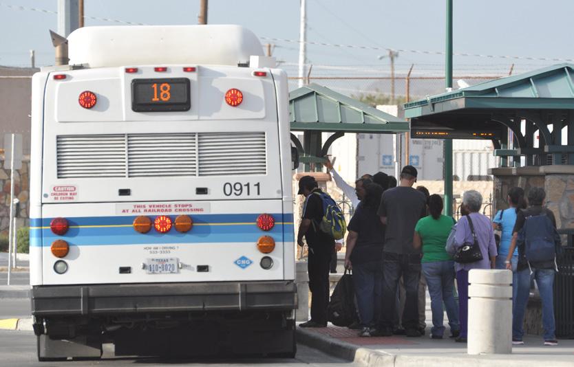
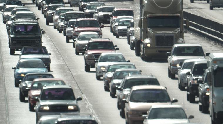
70 2012 URBAN MOBILITY REPORT David Schrank Bill Eisele Tim Lomax Texas A&M Transportation Institute POWERED BY REGION UNIVERSITY TRANSPORTATION CENTER