Process Modeling using UniSim Design

Transcription

1 Process Modeling using UniSim Design 4526/UDS Honeywell All rights reserved. UniSim is a U.S. registered trademark of Honeywell International Inc 4526.R380.02

2 Copyright The information in this training course is subject to change over time. Honeywell may make changes to the requirements described. Future revisions will incorporate changes, including corrections of typographical errors and technical inaccuracies. For further information please contact: Honeywell 5925 Centre Street SE Calgary, Alberta, CANADA T2H 0C2 Telephone: Web: Copyright Honeywell All rights reserved. UniSim is a U.S. registered trademark of Honeywell International Inc. Prepared in Belgium, Canada, Hungary and the United Kingdom.

3 Module Index 1. Getting Started 2. Propane Refrigeration Loop 3. Refrigerated Gas Plant 4. NGL Fractionation Plant 5. Oil Characterization 6. Two Stage Compression 7. Acid Gas Sweetening with DEA 8. Natural Gas Dehydration with TEG 9. Reporting with UniSim Design 10. Answers to Questions

4

5 Getting Started 1 Getting Started 2009 Honeywell All rights reserved. UniSim is a U.S. registered trademark of Honeywell International Inc R380.02

6 2 Getting Started 2

7 Getting Started 3 Workshop The Getting Started module introduces you to some of the basic concepts necessary for creating simulations in UniSim Design. You will use UniSim Design to define three gas streams to be used as feeds to a gas plant. In addition, you will learn how to determine properties of these streams by using the Phase Envelope and the Property Table utilities. Learning Objectives Define a fluid package (property package, components, hypotheticals) Add streams Understand flash calculations Attach stream utilities Customize the Workbook 3

8 4 Getting Started Simulation Basis Manager UniSim Design uses the concept of the fluid package to contain all necessary information for performing flash and physical property calculations. This approach allows you to define all information (property package, components, hypothetical components, tabular data, interaction parameters, reactions, etc.) inside a single entity. There are four key advantages to this approach: All associated information is defined in a single location, allowing for easy creation and modification of the data. Fluid packages can be stored as completely defined entities for use in any simulation. Component lists can be stored out separately from the Fluid Packages as completely defined entities for use in any simulation. Multiple Fluid Packages can be used in the same simulation, however, are all defined inside the common Basis Manager. The Simulation Basis Manager is a property view that allows you to create and manipulate multiple fluid packages or component lists in the simulation. The opening tab of the Simulation Basis Manager allows for the creation of component lists which are independent from fluid packages but can be associated with the individual fluid packages in the case. 4

9 Getting Started 5 The first tab of the Basis Manager allows you to manage the component list(s) used in your case. There are a number of buttons available: Figure 1 Button View Add Delete Copy Import Export Refresh Re-import Description Allows you to access the property view for the selected Component List. Allows you to create a Component List. Note: Component Lists can be added via the Fluid Package property view. Removes the selected Component List from the simulation. Makes a copy of the selected Component List. Allows you to import a predefined Component List from disk. Component Lists have the file extension (.cml). Allows you to export the selected Component List to disk. The exported Component List can be retrieved into another case, by using the Import function. Updates the pure component properties from the database. Allows you to re-import a cml file. Basis Environment icon You can use the Ctrl B hot key to re-enter the Simulation Basis Manager from any point in the simulation or click the Basis Environment icon from the tool bar. 5

10 6 Getting Started Inside the Current Fluid Packages group, there are a number of buttons: Figure 2 Button View Add Delete Copy Import Export Description This is only active when a fluid package exists in the case. It allows you to view the property view for the selected fluid package. Allows you to create and install a fluid package in the simulation. Removes the selected Fluid Package from the simulation. Makes a copy of the selected fluid package. Everything is identical in the copied version except the name. This is useful for modifying fluid packages. Allows you to import a predefined fluid package from disk. Fluid packages have the file extension (.fpk). Allows you to export the selected fluid package to a disk. The exported fluid package can be retrieved into another case by using the Import function. 6

11 Getting Started 7 Defining the Simulation Basis Add a Property Package 1. Start a new case by selecting the New Case icon. New Case icon 2. Go to the Fluid Pkgs tab and create a fluid package by clicking the Add button. 3. Scroll down the list and select the Peng-Robinson Equation of State model. Figure 3 You can select the EOS radio button in the Filter box, and then select Peng-Robinson; however, it is not necessary to select EOS after you have selected Peng-Robinson. 4. Change the Name from the default Basis-1 to GasPlant using the Name input box at the bottom of the window. 5. Click the View button in the Component List Selection section of the Set Up tab. This will allow you to add components to the Component List that is now associated with the GasPlant fluid package. 7

12 8 Getting Started Add Components You can select components for your simulation using several methods. You can add a range of components by highlighting the entire range and clicking the Add Pure button. Standard Windows list conventions (Shift = Select Range, Ctrl = Multi-Select) also work. To use... Component List Match Cell Filter Do this Using the scroll bar for the main component list, scroll through the list until you find the desired component. 2. To add the component, either: Press the ENTER key. Click the Add Pure button. Double-click on the component to add it to your simulation. 1. Select one of the three name formats, SimName, Full Name/Synonym, or Formula by selecting the corresponding radio button. 2. Click in the Match input field and enter the name of the component. As you start to type, the list will change to match what you have entered. 3. Once the desired component is highlighted, either: Click the ENTER key. Click the Add Pure button. Double-click on the component to add it to your simulation. 1. Ensure the Match cell is empty, and click the View Filter button. 2. Select the Use Filter checkbox to display the various family filters. 3. Select the desired family (e.g. Hydrocarbons) from the list of Family Filters to display only that type of component. 4. Use either of the two previous methods to then select the desired component. 6. Select the following library components, using one of the methods described above: Nitrogen H2S CO2 Methane Ethane Propane i-butane n-butane i-pentane n-pentane n-hexane H2O 8

13 Getting Started 9 Figure 4 7. Click on the Hypo Components\Traditional item in the Add Component box. Figure 5 When you click the Quick Create a Hypo Component button, UniSim Design adds a hydrocarbon class hypo by default. If you want to add a hypo from another class, click the Hypo Manager button and then in the view that appears, click the View Group button. This will open the Tabular Hypo Group input window, where you can add nonhydrocarbon class hypotheticals. 8. Click on the Quick Create a Hypo Component button to create a hypothetical component. A hypothetical component can be used to model non-library components, defined mixtures, undefined mixtures, or solids. You will be using a hypothetical component to model the components in the gas mixture heavier than hexane. 9. In the hypo component view, click on the ID tab and in the Component Name cell type C7+. 9

14 10 Getting Started Figure 6 UniSim Design always places an * after a hypo name so it can be distinguished from library components. Since you do not know the structure of the hypothetical component and you are modeling a mixture, the Structure Builder will not be used. 10. Click on the Critical tab. The only property supplied by the lab for the C7+ component is the Normal Boiling Pt; enter a value of 110 C (230 F). 11. Click the Est Unknown Props button to estimate all the other properties and fully define the hypothetical component. 10

15 Getting Started 11 Figure 7 The minimum information required for defining a hypo is the Normal Boiling Pt or the Molecular Weight and Ideal Liq Density. 12. When the hypo component has been defined, return to the fluid package by closing the hypo component C7+* view. 13. Add the hypo component to the Selected Components list by selecting it in the Available Hypo Components list and then clicking the Add Hypo button. Figure 8 When a component is added to the Selected Components list it appears above the currently selected component. You can use the Sort List button to order the Component List. 11

16 12 Getting Started Every hypo you create is part of a Hypo Group. By default, this hypo is placed in HypoGroup1. You can add additional groups and move hypo components between groups. This is done on the Hypotheticals tab of the Simulation Basis Manager. Compare the properties of C7+ with C7 and C8. Normal Boiling Point Ideal Liquid Density Molecular Weight C7+ C7 C8 You will need to add components C7 and C8 to the component list in order to view their properties. Ensure that you delete them once this exercise is finished. You have now finished defining the fluid package. You can view the Peng-Robinson binary coefficients for your selected components by selecting the Binary Coeffs tab on the Fluid Package tab. 12

17 Getting Started 13 Exporting Fluid Packages UniSim Design allows you to export fluid packages for use in other simulations. This functionality allows you to create a single common fluid package which you may then use in multiple cases. 14. On the Fluid Pkgs tab, highlight the GasPlant fluid package. Figure Click the Export button. 16. Enter a unique name ( GasPlant.fpk) for the fluid package and click the Save button. 13

18 14 Getting Started Figure 10 UniSim Design will automatically add the file extension.fpk when it saves your fluid package. The file is automatically saved to the \Paks folder of the UniSim Design installation directory. Enter Simulation Environment icon Now that the fluid package has been defined, you can start building the simulation. Click the Enter Simulation Environment button on the Simulation Basis Manager window to begin building the simulation. 14

19 Getting Started 15 Building the Simulation When you build the simulation, you will: Select a unit set Add streams, and specify them Attach utilities Select a Unit Set In UniSim Design, it is possible to change the unit set used to display its different variables. 1. From the Tools menu, choose Preferences. 2. Click on the Variables tab. Figure Select the SI unit set. 4. Close this view to return to the simulation. 15

20 16 Getting Started Adding Streams In UniSim Design, there are two types of streams, Material and Energy. Material streams have a composition and parameters such as temperature, pressure, and flow rates. They are used to represent process streams. Energy streams have only one parameter: heat flow. They are used to represent the duty supplied to or produced by a unit operation. There are a variety of ways to add streams in UniSim Design. To use this... Menu Bar Workbook Object Palette Do this... or From the Flowsheet menu select Add Stream. Press the F11 Hot Key. The Stream property view opens. Open the Workbook and go to the Streams tab. Type a stream name into the **New** cell. From the Flowsheet menu, select Open Object Palette or press F4 to open the Object Palette. Double-click on the stream icon. In this case, you will add three streams to represent three different gas wells. Each stream will be added using a different method of installation. Adding a Stream from the Menu Bar To add a stream using the F11 hot key: 1. Press F11. The stream property view appears. If the stream property view is not displayed, double-click on the newly created stream (from the PFD) to bring up the property view. 16

21 Getting Started 17 Figure Highlight the Stream Name cell. Change the stream name by typing in a new name: GasWell 1 and then press ENTER. Entering Stream Compositions Stream compositions are set via the Input Composition for Stream window but there are two different ways to access it. On this page... Conditions Composition Do this... or or Double-click on the Molar Flow cell to enter mole fractions. Double-click on the Mass Flow cell to enter mass fractions. Double-click on the Std Ideal Liquid Volume Flow cell to enter liquid volume fractions. The Input Composition for Stream view appears. Click the Edit button. The Input Composition for Stream view appears. 3. If the Input Composition for Stream view is not already open, double-click on the Molar Flow cell. 17

22 18 Getting Started Figure 13 The Normalize button sets any <empty> cells to 0 and adjusts the entered component fractions so that they sum to 1. The Equalize Composition button sets all compositions to Make sure the Mole Fractions radio button is set and enter the following compositions: Take care when closing the Input Composition for Stream view. Changes are only saved when OK is pressed. Any non-normalized compositions are automatically normalized when OK is pressed. For this component... Nitrogen H2S CO Methane Ethane Propane i-butane n-butane i-pentane n-pentane n-hexane C7+* H2O Enter this mole fraction Click the OK button when all the mole fractions have been entered 6. Close the Stream property view. 18

23 Getting Started 19 Adding a Stream from the Workbook To open the Workbook, click the Workbook icon on the tool bar. Workbook icon 1. Enter the stream name, GasWell 2 in the **New** cell. 2. Enter the following Molar compositions: For this component... Enter this mole fraction... Nitrogen H2S CO Methane Ethane Propane i-butane n-butane i-pentane n-pentane n-hexane C7+* H2O Click the OK button to close the Input Composition for Stream view. Material Stream icon (Blue) Adding a Stream from the Object Palette 1. If the Object Palette is not open on the Desktop, press F4 to open it. 2. Double-click on the Material Stream icon. A new stream is added to the flowsheet. Double-click on the new stream to access the Stream property view. 3. Change the name of the stream to GasWell Double-click on Molar Flow. 19

24 20 Getting Started 5. Enter the following stream compositions: For this component... Enter this mole fraction... Nitrogen H2S CO Methane Ethane Propane i-butane n-butane i-pentane n-pentane n-hexane C7+* H2O Click OK to close the Input Composition for Stream view. You can use one of several different methods to save a case in UniSim Design: Save Case icon From the File menu, select Save to save your case with the same name. From the File menu, select Save As to save your case in a different location or with a different name. Click the Save Case icon on the tool bar to save your case with the same name. 7. Click the Save Case icon, since this case doesnt yet have a file name, enter one (For example GettingStarted.usc) Save your case often to avoid the possibility of losing information. Save your case! 20

25 Getting Started 21 Changing Units for a Specification To change the units for a specification, simply type the numerical value of the specification and press the space bar, or click on the unit drop-down list. Choose the units for the value you are providing. UniSim Design will convert the units back to the default units. Figure 14 You can scroll through the unit list by starting to type the units, by using the arrow keys, or by using the scroll bar. To edit an existing value press F2 or use the small vertical bar to the left of the cell. 21

26 22 Getting Started Flash Calculations Only two of these five stream parameters (Vapour Fraction, Temperature, Pressure, Enthalpy and Entropy) can be supplied. UniSim Design can perform several types of flash calculations on streams. The most common types are Pressure-Temperature (P-T), Vapour Fraction-Pressure (Vf-P), and Vapour Fraction-Temperature (Vf-T). Once the composition of the stream and two of either, temperature, pressure or vapour fraction, are known, UniSim Design performs a flash calculation on the stream, calculating the other parameters. If you try to supply temperature, pressure and vapour fraction, a consistency error will occur. With the flash capabilities of UniSim Design, it is possible to perform dew and bubble point calculations. By specifying a vapour fraction of 1.0 and either the pressure or temperature of the stream, UniSim Design will calculate the dew point temperature or pressure. To calculate the bubble point temperature or pressure, a vapour fraction of 0.0 and either pressure or temperature must be entered. Perform a P-T flash calculation on the stream GasWell 2. Set the pressure to 7500 kpa and the temperature to 10 C. What is the vapour fraction? Perform a dew point calculation on the stream GasWell 2. Set the pressure to 7500 kpa. What is the dew point temperature? Perform a bubble point calculation on the stream GasWell 2. Set the pressure to 7500 kpa. What is the bubble point temperature? 22

27 Getting Started 23 Attaching Utilities The utilities available in UniSim Design are a set of useful tools that interact with your process, providing additional information or analysis of streams or operations. Once installed, the utility becomes part of the flowsheet, automatically recalculating when conditions change in the stream or operation to which it is attached. As with the majority of objects in UniSim Design, there are a number of ways to attach utilities to streams: To use the... Menu Bar Stream Property View Do this... From the Tools menu, select Utilities. or Press CTRL U. The Available Utilities view appears. 1. Open the Stream property view. 2. On the Attachments tab, click on the Utilities page. 3. Click the Create button. The Available Utilities view appears. Next, you will add a utility using each method of installation. Adding a Utility from the Stream Property View The Envelope Utility (in the Available Utilities list) allows you to examine relationships between selected parameters for any stream of known composition, including streams with only one component. Vapour-Liquid Envelopes may be plotted for the following variables: By default the phase envelope is calculated on a dry basis (any water is ignored). Pressure - Temperature Pressure - Volume Pressure - Enthalpy Pressure - Entropy Temperature - Volume 23

28 24 Getting Started Temperature - Enthalpy Temperature - Entropy An Envelope utility will be added to the stream GasWell 2 from the Stream property view. 1. Open the Stream property view for GasWell 2 by doubleclicking on the stream in either the Workbook or the PFD. 2. On the Attachments tab, click the Utilities page. Figure Click the Create button. The Available Utilities view appears. 4. Select Envelope Utility. Click the Add Utility button. The Envelope Utility view appears. 5. The Design tab shows the critical and maxima values for the envelope. What is the critical temperature and pressure for the stream GasWell 2? Tc Pc 6. Switch to the Performance tab to view the phase envelope. 24

29 Getting Started 25 Figure 16 Numerical values can be copied from UniSim Design to Microsoft Excel using the copy command, Ctrl+C, in UniSim Design, and then the paste command, Ctrl+V, in Excel. 7. Click the Table page to view envelope data in tabular format. Adding a Utility from the Menu Bar The Property Table Utility allows you to examine property trends over a range of conditions in both tabular and graphical formats. The utility calculates dependent variables for user specified independent variable ranges or values. A Property Table utility will be added to the stream Gas Well From the Tools menu select Utilities, or press CTRL U. The Available Utilities view appears. 2. Select Property Table. 3. Click the Add Utility button. The Property Table view appears. 25

30 26 Getting Started Figure Click the Select Stream button and select stream GasWell Click the OK button to return to the Design tab. 6. In the Independent Variables section, select Pressure as the first Independent Variable. 7. Change the mode to State, use the drop-down menu bar. 8. In the State Values matrix, enter values of 2500, 5000, 7500, and 9000 kpa. If you are using field units, the values will be 350, 700, 1050 and 1400 psia. 9. Choose Temperature as the second Independent Variable. Ensure the mode is set to Incremental. 10. Change the Lower and Upper Bounds to 0 C (32 F) and 100 C (212 F) respectively. Leave # of Increments at the default value of

31 Getting Started 27 Figure On the Design tab, click on Dep. Prop. 12. On the Dep. Prop page, click on the Add button. 13. Choose Mass Density from the list. Click OK to accept. 14. Click on the Add button again. Select the Thermal Conductivity and click OK to accept. 15. Click the Calculate button to generate the property table. 16. Examine the property table results in either graphical or tabular format on the Performance tab. Figure 19 27

32 28 Getting Started Analyzing the Results Stream Property View Within UniSim Design, it is possible to view the properties of the individual phases for any stream. 1. Open the Stream property view for GasWell 3 by doubleclicking on GasWell 3 in the PFD, and view the Conditions page. 2. Add Temperature and Pressure values of -20 C (-4 F) and 5000 kpa (725 psia). 3. Move the mouse arrow to the left or right side of the view until the arrow changes to the double-headed resizing arrows. 4. Press and hold the left mouse button and drag the edge of the view until all the phases can be seen as shown below. Figure 20 28

33 Getting Started Go to the Properties page. This page contains more detailed information about the stream. Figure Close the worksheet for GasWell 3. 29

34 30 Getting Started Customizing the Workbook Workbook icon UniSim Design allows you to customize the Workbook at several different levels. You can add additional pages, change the variables which are displayed on the current pages, or change the format of the values. In this exercise, a new Workbook tab containing stream properties, Cp/Cv, Heat of Vapourization, and Molar Enthalpy will be added. 1. Open the Workbook by clicking the Workbook icon on the tool bar. 2. From the Workbook menu, select Setup. The Setup view appears as shown below. Figure 22 The Workbook menu only appears when the Workbook window is active. If the PFD window is active it is replaced by the PFD menu. 3. Under the Workbook Tabs group, click the Add button. The New Object Type view appears. 30

35 Getting Started 31 Figure Select Stream and click OK. 5. A new Workbook tab, Streams, will be listed in the Workbook Tabs group. Ensure that this new tab is highlighted. 6. Highlight the Name cell and change the name to Other Props. 7. In the Variables group, click the Delete button until all the default variables are removed. 8. Click the Add button to add a new variable to the tab. 9. From the Variable list, select Cp/Cv and click OK. 10. Repeat steps #8 and #9 to add Mass Heat of Vapourization and Molar Enthalpy as shown below. 31

36 32 Getting Started Figure When complete close the Setup view to return to the Workbook. 12. The Workbook now contains the tab Other Props which shows the values of Cp/Cv, Mass Heat of Vapourization, and Molar Enthalpy as shown below. Figure 25 32

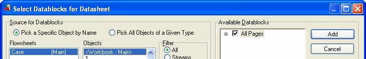
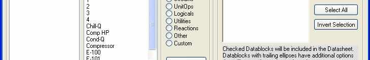
37 Getting Started 33 Printing Stream & Workbook Datasheets In UniSim Design you have the ability to print Datasheets for streams, operations, and Workbooks. Printing the Workbook Datasheet 1. Open the Workbook. Workbook icon 2. Right-click (object inspect) the Workbook title bar. The Print Datasheet pop-up menu appears. Figure Select Print Datasheet. The Select Datablock view appears. 33

38 34 Getting Started Figure 27 The Workbook Datasheet can be used to print a report for all the streams or a subset. To do this: If required, use the Order/Hide/Reveal Objects option on the Workbook menu to limit the streams displayed. Customize the Workbook to contain all the stream data you want. Print the Workbook Datasheet. 4. From the list, you can choose to print or preview any of the available datasheets. Printing an Individual Stream Datasheet To print the datasheet for an individual stream, object inspect the stream property view title bar and follow the same procedure as for the Workbook. 34

39 Getting Started 35 Finishing the Simulation The final step in this section is to add the stream information necessary for the case to be used in future modules. Add the following temperature, pressure, and flow rate to the streams: Stream Temperature Pressure Flow Rate GasWell 1 GasWell 2 GasWell 3 40 C (105 F) 4135 kpa (600 psia) 425 kgmole/h (935 lbmole/hr) 45 C (113 F) 3450 kpa 375 kgmole/h (500 psia) (825 lbmole/hr) 45 C (113 F) 575 kgmole/h (1270 lbmole/hr) Save your case! 35

40 36 Getting Started Exploring the Simulation Exercise 1: Phase Behavior & Hydrate Prediction A. Use the Phase Envelope to answer the following questions: Critical Point for GasWell 1. Cricondenbar (maximum pressure) for GasWell 1. Bubble Point temperature for GasWell 3 at 6000 kpa. Dew Point temperature for GasWell 1 at 4000 kpa. GasWell 1 temperature for 50% quality at 8000 kpa. Hydrate Formation temperature for GasWell 2 at 7500 kpa. 36

41 Getting Started 37 B. Use the Workbook to find the following values: Bubble Point temperature for GasWell 3 at 6000 kpa. Dew Point temperature for GasWell 1 at 4000 kpa. GasWell 1 temperature for 50% quality at 8000 kpa. C. Use the Hydrate Formation Utility to find the hydrate formation temperature for GasWell 1 and GasWell 2. Stream Pressure, kpa (psia) Hydrate Temperature GasWell (725) GasWell (1090) GasWell (725) GasWell (1090) 37

42 38 Getting Started Challenge By default the phase envelope utility only performs the flash calculations on a dry basis, it will ignore any water present in the stream. The envelope utility can perform a calculation including the effect of water if the UniSim Thermo Three-Phase option is chosen from combobox at the top right of the Connections page. The composition of GasWell 3 contains some water. You have been asked to perform a number of Dew and Bubble Point calculations on the stream at various pressures. Knowing that you cannot accurately predict these points on the Phase Envelope (because of the water) you start to do the calculations in the Workbook. After about 30 minutes of doing flashes and writing down the pressure-temperature values, your colleague comes in and tells you the wonders of the Property Table and you are done in about five minutes. Following your colleagues advice, set up a Property Table to generate a Bubble Point curve and Dew Point curve from 100 to kpa. Note: If you make any changes to the temperature and pressure of the streams, be sure to reset them to the values given in the Finishing the Simulation section above before saving your case. 38

43 Propane Refrigeration Loop 1 Propane Refrigeration Loop 2009 Honeywell All rights reserved. UniSim is a U.S. registered trademark of Honeywell International Inc R380.02

44 2 Propane Refrigeration Loop 2

45 Propane Refrigeration Loop 3 Workshop Refrigeration systems are commonly found in the natural gas processing industry and in processes related to the petroleum refining, petrochemical, and chemical industries. Refrigeration is used to cool gas to meet a hydrocarbon dew point specification and to produce a marketable liquid. In this module you will construct, run, analyze, and manipulate a propane refrigeration loop simulation. You will convert the completed simulation to a template, making it available to connect to other simulations. Learning Objectives Once you have completed this module, you will be able to: Add and connect operations to build a flowsheet Use the graphical interface to manipulate flowsheets in UniSim Design Understand forward-backward information propagation in UniSim Design Convert simulation cases to templates Prerequisites Before beginning this module, you need to know how to: Define a fluid package Define streams Navigate the Workbook interface 3

46 4 Propane Refrigeration Loop 4

47 Propane Refrigeration Loop 5 Building the Simulation The first step in building any simulation is defining the fluid package. A brief recap on how to define a fluid package and install streams is described below. (For a complete description, see the previous module). Defining the Simulation Basis 1. Create a New Case and add a fluid package. 2. Enter the following values in the specified fluid package view: On this page... Property Package Components Select... Peng-Robinson Propane Enter Simulation Environment icon 3. Click Enter Simulation Environment button when you are ready to start building the simulation. Installing a Stream There are several ways to create streams. (For a complete description, see the previous module.) Press F11. The Stream property view appears. or Double-click the Stream icon in the Object Palette. Defining Necessary Streams Add a stream with the following values: 5

48 6 Propane Refrigeration Loop In this cell Enter Name 1 Vapour Fraction 0.0 Temperature 50 C (120 F) Composition Propane - 100% Add a second stream with the following properties: In this cell Enter Name 3 Vapour Fraction 1.0 Temperature -20 C (-4 F) What is the pressure of Stream 1? Adding Unit Operations to a Flowsheet As with streams, there are a variety of ways to add unit operations in UniSim Design: To use the Menu Bar Workbook Object Palette PFD/Object Palette Do this or From the Flowsheet menu, select Add Operation Press F12. The UnitOps view appears. Open the Workbook and go to the UnitOps page, then click the Add UnitOp button. The UnitOps view appears. or From the Flowsheet menu, select Palette Press F4. Double-click the icon of the unit operation you want to add. Using the right mouse button, drag n drop the icon from the Object Palette to the PFD. 6

49 Propane Refrigeration Loop 7 The propane refrigeration loop consists of four operations: Valve Chiller Compressor Condenser In this exercise, you will add each operation using a different method of installation. Adding a J-T Valve The J-T Valve is modeled using the Valve operation in UniSim Design. The inlet to the valve comes from the condenser outlet. The condenser outlet is at its bubble point. The valve will be added using the F12 hot key. You can filter the Available Unit Operations list by selecting an appropriate Category. In this case, Piping Equipment would filter the list to include the Valve operation. 1. Press F12. The UnitOps view appears: Figure 1 2. Select Valve from the Available Unit Operations list. 3. Click the Add button. The Valve property view appears. 4. On the Connections page, supply the inlet and outlet connections as shown below: 7

50 8 Propane Refrigeration Loop Figure 2 Drop-down lists, such as for the Feed and Product streams, contain lists of available streams which can be connected to the operation. Adding a Chiller The Chiller operation in the propane loop is modeled in UniSim Design using a Heater operation. The outlet of the Chiller will be at its dew point. To add a heater: 1. Open the Workbook and click the Unit Ops tab. 2. Click the Add UnitOp button. The UnitOps view appears. 3. Select Heat Transfer Equipment from the Categories group. 4. Select Heater from the Available Unit Operations list as shown below. 8

51 Propane Refrigeration Loop 9 Figure 3 5. Click the Add button, or double click on Heater. The Heater property view appears. 6. On the Connections page, enter the information as shown below: Figure 4 7. Go to the Parameters page. 9

52 10 Propane Refrigeration Loop 8. Enter a Delta P value of 7.0 kpa (1 psi) and a Duty value of 1.00e+006 kj/h (1.00e+06 Btu/hr) for the Chiller. Figure 5 The Parameters page will be common to most unit operations and contains parameters such as Delta P, Duty, and Efficiency. 9. Close the property view. What is the molar flow rate of propane? What is the pressure drop across the J-T valve? What is the temperature of the valve outlet (stream 2)? Adding a Compressor Compressor icon The Compressor operation is used to increase the pressure of an inlet gas stream. To add a compressor: 1. Press F4. The Object Palette appears. 2. Double-click the Compressor icon on the Object Palette. The Compressor property view appears. 3. On the Connections page, enter the stream information as shown below: 10

53 Propane Refrigeration Loop 11 Figure 6 4. Complete the Parameters page as shown below: Figure 7 Adding the Condenser The Condenser operation completes the propane refrigeration loop. It is placed between the Compressor and the Valve and is modeled as a Cooler operation. 11

54 12 Propane Refrigeration Loop Working with a graphical representation, you can build your flowsheet in the PFD using the mouse to install and connect objects. This procedure describes how to install and connect the Cooler using the Object Palette drag n drop technique. Using Drag n Drop in the PFD 1. Click the Cooler icon on the Object Palette. Cooler icon 2. Move the cursor to the PFD. The cursor will change to a special cursor, with a box and a plus (+) symbol attached to it. The box indicates the size and location of the cooler icon. 3. Click again to drop the cooler onto the PFD. There are two ways to connect the operation to a stream on the PFD: To connect using the Attach Mode toggle CTRL key Do this 1. Press the Attach Mode toggle button on the PFD button bar. 2. Place the cursor over the operation. The connection points are highlighted as squares and rectangles. Material stream connections are dark blue, energy stream connections are red. 3. Move the cursor over the connection you want to make. When over the connection the cursor icon changes to one with a white square, and a pop up message tells you which connection it is. 4. Press and hold the left mouse button. 5. Move the cursor to the stream icon you wish to connect, if a connection is allowed a square connection point appears. 6. Move the cursor over the connection point and release the mouse button. 1. Press and hold the CTRL key, notice that the Attach Mode button appears depressed. 2. Follow the same steps as above 3. When complete, release the CTRL key. 4. From the PFD, connect stream 4 to the Condenser inlet and connect the Condenser outlet to stream 1 using one of the methods in the table above. 5. Double-click on the Condenser. 6. On the Parameters page, enter a Delta P of 35 kpa (5 psi). 12

55 Propane Refrigeration Loop 13 Figure 8 Hint: Clone a unit set and set the Power to hp units. What is the compressor energy in hp? Save your case! 13

56 14 Propane Refrigeration Loop Undo/Redo/Recent Values UniSim Design offers an undo/redo facility. It applies in the following circumstances: Values entered into object property values (streams/unit operations) PFD object moves and resizing Object Property Views In any object property view (e.g. a material stream or any unit operation) UniSim Design has an unlimited undo/redo feature. To use undo/redo use the Undo and Redo options on the Edit menu or the short cut keys CTRL Z and CTRL Y. Figure 9 Additionally by right clicking on any specified value a list of all recent entered values can be entered. 14

57 Propane Refrigeration Loop 15 Figure 10 Note that any undo/redo/recent values information is lost when the object property view is closed. Each time an object property view is opened fresh undo/redo/recent values information is stored. Note also that using the undo/redo/recent values facility has the same effect as typing the value in the cell; any other parts of the flowsheet that depend on the value will recalculate accordingly. PFD object moves and resizing UniSim Design also has an unlimited undo/redo facility for object moves and object resizing on the PFD. This is also accessed by the Undo and Redo options on the Edit menu or the short cut keys CTRL Z and CTRL Y. Note that any undo/redo information is lost when the PFD window is closed. Each time a PFD window is opened fresh undo/redo information is stored. Note also that you cannot undo object deletion. 15

58 16 Propane Refrigeration Loop Manipulating the PFD The PFD is designed around using the mouse and/or keyboard. There are a number of instances in which either the mouse or the keyboard can be used to perform the same function. One very important PFD function for which the keyboard cannot be used is object inspection. You can perform many of the possible tasks and manipulations on the icons in the PFD by using object inspection. Place the mouse arrow over the object you want to inspect and press the right mouse button. An appropriate menu is produced depending upon the object selected (Stream, Streamline, Operation, Column, PFD Table, PFD Background, Text Annotation etc.). A list of the objects that you can object inspect are shown in the following table with the corresponding menus. Object PFD Object Inspection Menu Text Annotations 16

59 Propane Refrigeration Loop 17 Object Unit Operations Object Inspection Menu Unit Operation Tables Workbook Tables Streams (Depending on where on the stream you click, either of these two menus will appear. To see the long menu, rightclick on the stream icon. To see the short menu, right-click on the stream line). 17

60 18 Propane Refrigeration Loop Customize the PFD by performing the following: Add Text icon The width of the text box is modified by clicking the Size Mode button on the PFD button bar and then clicking on the text box. Click on either white square that appears on the left and right side of the text box and drag to desired width. 1. Add the Title: Propane Refrigeration Loop by clicking the Add Text icon on the PFD tool bar. Move the cursor to an appropriate location on the PFD where the text should be displayed and left-click the mouse button. Type the title text in the Text Props View that appears and click OK. Modify the title color, font and size from the options available in the Text Annotations menu. Hint: right-click on the title to see this menu. 2. Add a Workbook Table for the material streams in the simulation. Hint: right click on the PFD background and use the Add Workbook Table option. 3. Add a Table for Stream 4. Hint: right-click on Stream 4 Note that existing tables can be modified by double clicking on them and making the desired changes. Save your case! 18

61 Propane Refrigeration Loop 19 Saving the Simulation as a Template A template is a complete flowsheet that has been stored to disk with additional information included so that the flowsheet can be added to another model as a sub-flowsheet operation. Typically, a template is representative of a plant process module or portion of a process module. The stored template can subsequently be read from disk and efficiently installed as a complete subflowsheet operation any number of times into any number of different simulations. Some of the advantages of using templates are: Provides a mechanism by which two or more cases can be linked together Employs a different property package than the main case to which it is attached Provides a convenient method for breaking large simulations into smaller, easily managed components Is created once and can be installed in multiple cases Before you convert the case to a template, it needs to be made generic so it can be used with gas plants of various flow rates. In this case, the Chiller Duty dictates the flow rate of propane required. 1. Delete the Chiller Duty value. 2. From the Simulation menu, select Main Properties. The Simulation Case view appears as shown below. 19

62 20 Propane Refrigeration Loop Figure Click the Convert to Template button. 4. Click Yes to convert the simulation case to a template. 5. Answer No to the question Do you want to save the simulation case. 6. Go to the File menu and Save the template as C3Loop.utpl. 20

63 Propane Refrigeration Loop 21 Analyzing the Results This section describes how to retrieve and print unit operation results. Printing Datasheets for Unit Operations To set up the printer, select Printer Setup from the File menu, then select either the Graphic Printer or the Report Printer. This allows you to set the printer configuration: printer, paper, size, source and orientation. In UniSim Design you can print results through: The menu bar Object inspection of unit operations The Report Manager Printing Using the Menu Bar Choose one of the following options from the File menu: Print. Lists the available Datasheets for the active unit operation. You can highlight a Datasheet and either preview or print it. Figure 12 Choosing the Print command when the PFD is the active view will print the PFD. There are no datasheets available for the PFD. Print Window Snapshot. Prints a bitmap of the active UniSim Design view. 21

64 22 Propane Refrigeration Loop Printing Using Object Inspection Object inspect the Title Bar of the unit operation property view and select Print Datasheet. A list of available Datablocks is displayed for the object. Printing Using Report Manager 1. Open the Tools menu. Select Reports. The Report Manager view appears as shown below. Figure Click the Create button to add a new report. The Report Builder view appears as shown below. Figure Click the Insert Datasheet button to add datasheets to your report. You can add single or multiple unit operation Datasheets to a report. 22

65 Propane Refrigeration Loop 23 Figure 15 23

66 24 Propane Refrigeration Loop Adding Unit Operation Data to the Workbook Each WorkBook has a Unit Ops page by default that displays all the unit operations and their connections in the simulation. You can add additional pages for specific unit operations to the WorkBook. For example, you can add a page to the WorkBook that contains only the compressors in the simulation. Adding a Unit Operation Tab to the WorkBook 1. Open the WorkBook. Open the WorkBook menu. Select Setup. The Setup view appears. 2. Click the Add button in the Workbook Tabs group. The New Object Type view appears. Double-clicking on an entry with a + sign will open an expanded menu. 3. Select Rotating Equipment and expand the list. Select Compressor as shown. Figure Click OK. A new page, Compressors, containing only compressor information is added to the WorkBook. 5. Close this view. 24

67 Propane Refrigeration Loop 25 Adding Unit Operation Data to the PFD For each unit operation, you can display a Property Table on the PFD. The Property Table contains certain default information about the unit operation. Adding Unit Operation Information to the PFD 1. Open the PFD. Remember you can Object Inspect an object by selecting it and then clicking on it with the right mouse button. 2. Select the unit operation for which you want to add the Property Table. 3. Object Inspect the unit operation. 4. Click Show Table. 5. After the table has been added, you can move it by selecting it and dragging it with the mouse. 6. If you Object Inspect the table, you can change its properties and appearance. You can also specify which variables the table will show. 25

68 26 Propane Refrigeration Loop Advanced Modeling One of the key design aspects of UniSim Design is how Modular Operations are combined with a Non-Sequential solution algorithm. Not only is information processed as you supply it, but the results of any calculation are automatically propagated throughout the flowsheet, both forwards and backwards. The modular structure of the operations means that they calculate in either direction, using information in an outlet stream to calculate inlet conditions. This design aspect is illustrated using the Propane Refrigeration Loop. Figure 17 Initially, the only information supplied in the case is the temperature and vapour fraction for streams 1 and 3 and the composition of stream 1. Since the temperature, vapour fraction, and composition of stream 1 are known, UniSim Design will automatically perform a flash calculation and determine the remaining properties (pressure, intensive enthalpy, density, etc.) which are independent of flow. When streams 1 and 2 are attached to the valve J-T, UniSim Design first determines what information is known in either the input or output stream. It will then assign these values to the other stream. In this case, since no valve pressure drop was specified, only the composition and intensive enthalpy of stream 1 will be passed to stream 2. 26

69 Propane Refrigeration Loop 27 By attaching stream 2 and 3 to the heater operation, Chiller, the composition of stream 2 is passed to stream 3 (100% Propane). UniSim Design can now perform a flash calculation on stream 3 and determine the remaining properties which are independent of flow, i.e. pressure, enthalpy, etc. Using the calculated pressure of stream 3 and the specified pressure drop across the heater, UniSim Design back calculates the pressure of stream 2. Since pressure, composition and intensive enthalpy of stream 2 are now known (the valve is isenthalpic), UniSim Design can calculate the temperature of stream 2. In addition, UniSim Design uses the specified heater duty and the intensive enthalpy of streams 2 and 3 to calculate the flow rate, which is then passed on to streams 1, 2 and 3. Next, the Compressor is added to the simulation. Since all of the inlet information is known, the compressor has only 2 degrees of freedom remaining. Parameters such as Efficiency, Duty, or Outlet Pressure can satisfy one degree of freedom. The second degree of freedom comes from the Condenser. The Condenser connects the Compressor outlet to the Valve inlet (which is completely defined). The user supplies the Condenser pressure drop, and UniSim Design calculates the inlet pressure, which is also the Compressor outlet pressure (the second degree of freedom for the Compressor). 27

70 28 Propane Refrigeration Loop Exploring the Simulation Use your saved case (not the template) for the following exercises. Exercise 1: Design vs. Rating Scenarios In the plant, you are unable to accurately measure or calculate the chiller duty. You do, however, know that the compressor is rated for 250 hp and that it is running at 90% of maximum and 72% efficiency. What is the chiller duty? The Chiller Gas Flow meter has finally been calibrated and you can determine the chiller duty. It has been decided to increase the chiller duty to 1.5 MMBTU/hr. With the compressor running at the same horsepower (225 hp), what is the best chiller outlet temperature you can achieve (and thus maximize cooling for the process) while still running the compressor at a reasonable operating point? 28

71 Propane Refrigeration Loop 29 Exercise 2: Refrigerant Composition Before starting this exercise return the refrigeration loop to its original configuration: Chiller duty specified (1.00e+006 kj/h), compressor adiabatic efficiency specified (75%) and power calculated, chiller outlet temperature specified (-20 C). Your local propane dealer arrives at your plant selling a 95/5 (mole%) Propane/Ethane blend. What effect, if any, does this new composition have on the refrigeration loop? Use the base case for comparison: Flow, kgmole/h Condenser Q, kj/h Compressor Q, hp Base Case: 100% Propane New Case: 5% Ethane, 95% Propane 29

72 30 Propane Refrigeration Loop Challenge: Adding an Economizer Create a two stage refrigeration loop by adding an Economizer. What is the net compression in hp? Figure 18 Add the following specifications to the refrigeration loop: For this Item Add this specification Stream 1 T = 50 C and Vf = 0.0 Chiller Stream 3 Stream 4 Mixer Condenser Pressure Drop = 7 kpa Q = 1.0e+006 kj/h T = -20 C Vf = 1.0 P = 625 kpa Equalize All Pressures Pressure Drop = 35 kpa Save your case! 30

73 Refrigerated Gas Plant 1 Refrigerated Gas Plant 2009 Honeywell All rights reserved. UniSim is a U.S. registered trademark of Honeywell International Inc R380.02

74 2 Refrigerated Gas Plant 2

75 Refrigerated Gas Plant 3 Workshop In this simulation, a simplified version of a refrigerated gas plant will be modeled. The purpose is to find the LTS (Low Temperature Separator) temperature at which the hydrocarbon dew point target is met. The Sales Gas hydrocarbon dew point should not exceed -15 C at 6000 kpa. The incoming gas is cooled in two stagesfirst by exchange with product Sales Gas in a gas-gas exchanger (Gas- Gas) and then in a propane chiller (Chiller), represented here by a Cooler operation. A Virtual Stream operation will be used to evaluate the hydrocarbon dew point of the product stream at 6000 kpa. Learning Objectives Once you have completed this section, you will be able to: Install and converge heat exchangers Understand logical operations (Virtual Stream and Adjust) Use the Case Study tool to perform case studies on your simulation Prerequisites Before beginning this section you need to know how to: Create a fluid package Add streams Add unit operations 3

76 4 Refrigerated Gas Plant 4

77 Refrigerated Gas Plant 5 Building the Simulation Three tasks are required to build the simulation: 1. Defining component list and fluid package 2. Adding streams and unit operations 3. Adding logical operation (Virtual Stream and Adjust) Defining the Simulation Basis For this case, you will be using the Peng-Robinson EOS with the following components: Nitrogen H2S CO2 Methane Ethane Propane i-butane n-butane i-pentane n-pentane n-hexane H2O C7+* 1. Create a New Case. If you want to re-create the fluid package, refer to the first module (Getting Started). 2. On the Fluid Pkgs tab import the fluid package, GasPlant.fpk, which you saved in Module 1 (Getting Started). Adding a Feed Stream Add a new Material stream with the following values: 5

78 6 Refrigerated Gas Plant In this cell Name Temperature Pressure Enter To Refrig 15 C (60 F) 6200 kpa (900 psia) Flow Rate 1440 kgmole/h (3175 lbmole/hr) Component Mole Fraction Nitrogen H2S CO Methane Ethane Propane i-butane n-butane i-pentane n-pentane n-hexane H2O 0 C7+* Adding a Separator There are several ways to add unit operations. For a complete description, see the Propane Refrigeration Loop module (Adding Unit Operations to a Flowsheet section). Press the F12 hot key. Select the desired unit operation from the Available Unit Operations group. Double-click the unit operation button in the Object Palette. On the Connections tab, add a Separator and enter the following information: In this cell... Name Feed Vapour Outlet Liquid Outlet Enter... Inlet Gas Sep To Refrig Inlet Sep Vap Inlet Sep Liq 6

79 Refrigerated Gas Plant 7 Adding a Heat Exchanger Heat Exchanger icon The heat exchanger performs two-sided energy and material balance calculations. The heat exchanger is capable of solving for temperatures, pressures, heat flows (including heat loss and heat leak), material stream flows, and UA. 1. Double-click the Heat Exchanger button on the Object Palette. 2. On the Connections page, enter the following information: Figure 1 The Tube Side and Shell Side streams can come from different Flowsheets, so for example, you can use Steam Tables for the fluid package on one side of the exchanger and Peng-Robinson on the other side. 3. Switch to the Parameters page. Complete the page as shown in the following figure. The pressure drops for the Tube and Shell sides will be 35 kpa (5 psi) and 5 kpa (1 psi), respectively. 7

80 8 Refrigerated Gas Plant Figure 2 The heat exchanger models are defined as follows: Weighted. The heating curves are broken into intervals, which then exchange energy individually. An LMTD and UA are calculated for each interval in the heat curve and summed to calculate the overall exchanger UA. The Weighted method is available only for Counter-Current exchangers. Endpoint. A single LMTD and UA are calculated from the inlet and outlet conditions. For simple problems where there is no phase change and Cp is relatively constant, this option may be sufficient. 4. Go to the Specs page. To solve the heat exchanger, unknown parameters (flows, temperatures) are manipulated by the solver. Each constraint (specification) will reduce the degrees of freedom by one. The number of constraints (specifications) must equal the number of unknown variables. When this is the case, the degrees of freedom will be equal to zero, and a solution will be calculated. 8

81 Refrigerated Gas Plant 9 Two specifications are needed for this exchanger: You can have multiple Estimate specifications. The Heat Exchanger will only use the Active specifications for convergence. Heat Balance = 0. This is a Duty Error specification and is needed to ensure that the heat equation balances. This is a default specification that is always added by UniSim Design so you do not need to supply it. Min Approach = 5 C. This is the minimum temperature difference between the hot and cold stream. 5. You will first need to deactivate the UA specification. To do this, uncheck the Active checkbox for the UA specification. Figure 3 6. To add a specification, click the Add button, the ExchSpec view appears. Figure 4 7. Provide the following information: 9

82 10 Refrigerated Gas Plant In this cell... Name Type Pass Spec Value Enter... Temp Approach Min Approach Overall 5 C (9 F) When you change the type of specification, the view will change accordingly. Once all the information has been provided, the view will be as shown below: Figure 5 What is the flow rate of Gas to Chiller? 10

83 Refrigerated Gas Plant 11 Finishing the Simulation Add the two remaining physical unit operations to complete the simulation. 1. Add a Cooler and provide the following information: In this cell Connections Name Inlet Stream Outlet Stream Energy Stream Parameters Delta P Enter Chiller Gas to Chiller Gas to LTS Chiller Q 35 kpa (5 psia) 2. Add a Separator and provide the following information on the Connections tab: In this cell Name Inlet Stream Vapour Outlet Liquid Outlet Enter LTS Gas to LTS LTS Vap LTS Liq What piece of information is required for the LTS separator to solve? 11

84 12 Refrigerated Gas Plant In the next section the LTS feed temperature will be varied using an Adjust operation to find a temperature at which the dew point constraint is met. For now, specify the temperature of stream Gas to LTS to be -20 C (-4 F). What is the pressure of Sales Gas? What is the temperature of Sales Gas? 12

85 Refrigerated Gas Plant 13 Adding a Virtual Stream Virtual Stream icon The Virtual Stream operation provides a general purpose facility to create a live copy of the data from one stream (the Reference stream) to another (the Target stream). The Reference and Target streams must be specified on the Connections tab. The Virtual Stream operation may also be used in other cases, for example, to perform flash calculations. Figure 6 The Virtual Stream is classified with the logical operations on the Object Palette. The Virtual Stream operation shows green connections because it does not imply a material balance. To make a duplicate of a stream, four reference variables must be selected in the Transfer Information section of the Parameters tab as depicted in Figure 7 below. Composition must be selected, flow (molar or mass) and two of either: vapour fraction, temperature, pressure and enthalpy. Selecting pressure and enthalpy as the last two variables will define the stream uniquely. Note backward translation from the Target Stream to the Reference Stream is also possible if the corresponding property of the reference stream is deleted and the property of the target stream is specified instead. 13

86 14 Refrigerated Gas Plant Figure 7 In order to use the Virtual Stream operation to perform flash calculations, composition and flow (molar or mass) must be selected in the Transfer Information area of the Virtual Stream Parameters tab. The user will specify the flash variables, vapour fraction, pressure and/or temperature, depending on whether dew or bubble point calculations are the desired target. 1. Double-click on the Virtual Stream icon on the Object Palette. 2. Add the following information on the Connections tab: In this cell... Reference Stream Target Stream Enter... Sales Gas HC Dew Point 3. Go to the Parameters tab. The Virtual Stream operation translates stream data using a multiplier and offset per the following linear formula: Y = M*X + B M=Multiplier, B=Offset Y is the Target stream data, and X is the Reference stream data. 4. Select composition and flow (molar or mass). 5. Specify a Pressure of 6000 kpa (870 psia) for the stream HC Dew Point, and set the Vapour Fraction to calculate the dew point temperature. This can be done on the Parameters tab of the Virtual Stream (Target Value), or on the Worksheet tab of the HC Dew Point stream itself. Observe that entering the values in one will populate the other. 14

87 Refrigerated Gas Plant 15 Figure 8 What is the dew point temperature? The required dew point is -15 C, is the current dew point higher or lower? Assuming pressure is fixed, what other parameter affects the dew point? How can we change the dew point in the simulation? 15

88 16 Refrigerated Gas Plant Adding the Adjust Adjust icon The Adjust operation is a Logical Operation; a mathematical operation rather than a physical operation. It will vary the value of one stream variable (the independent variable) to meet a required value or specification (the dependant variable) in another stream or operation. 1. Double-click on the Adjust icon on the Object Palette, the Adjust property view appears. Figure 9 The Adjusted Variable must always be a userspecified value. 2. Click the Select Var... button in the Adjusted Variable group. The Variable Navigator view appears. 3. From the Object list, select Gas to LTS. From the Variable list which is now visible, select Temperature. 16

89 Refrigerated Gas Plant 17 Figure 10 Always work left to right in the Variable Navigator. Dont forget you can use the Object Filter when the Object list is large. 4. Click the OK button to accept the variable and return to the Adjust property view. 5. Click the Select Var... button in the Target Variable group. 6. Select the object HC Dew point, and then select Temperature as the target variable. 7. Click the OK button to accept the variable and return to the Adjust property view. 8. Enter a value of -15 C (5 F) in the Specified Target Value box. 9. The completed Connections tab is shown below. 17

90 18 Refrigerated Gas Plant Figure Switch to the Parameters tab, and leave the parameters at the default values: Figure 12 When adjusting certain variables, it is often a good idea to provide a minimum or maximum which corresponds to a physical boundary, such as zero for pressure or flow. 18

91 Refrigerated Gas Plant 19 Note the Tolerance and Step Size values. When considering step sizes, use larger rather than smaller sizes. The Secant method works best once the solution has been bracketed and by using a larger step size, you are more likely to bracket the solution quickly. 11. Click the Start button to begin calculations. 12. To view the progress of the Adjust, go to the Monitor tab. Figure 13 What is the Chiller outlet temperature to achieve the dew point specification? Save your case! 19

92 20 Refrigerated Gas Plant Choosing the Adjust Method In Sequential (i.e. Non-simultaneous) mode the Adjust has a choice of three methods: The Modified Secant method was introduced in UniSim Design R380. Secant (default) Broyden Modified Secant In general the Secant is slower but more reliable than the Broyden method. The Modified Secant method includes several enhancements over the original Secant method: More efficient control of internal variable bounds and step size. Better able to find a bracket for the solution. Reverts to Bi-Section search if unable to find a solution otherwise. When the calculation is stuck at one variable bound, it will switch to the other bound and continue calculations. In combination this method allows the Adjust to better cope with the situation where the target variable is invariant over a portion of the adjusted variable range. The Modified Secant method is a good general purpose choice. 20

93 Refrigerated Gas Plant 21 Advanced Modeling Linking the Propane Loop to the Gas Plant Sub-Flowsheet icon Once you have completed the Refrigerated Gas Plant example, you can link it to the Propane Loop template. The Chiller duty, Chiller Q, in the Gas Plant will be linked to the Chiller duty, Chill-Q, in the Propane Refrigeration Loop template. 1. Using the Refrigerated Gas Plant simulation constructed above double-click on the Sub-Flowsheet icon on the Object Palette. 2. Click the Read an Existing Template button. 3. Open the template file saved in Module 2, C3Loop.utpl. 4. In the Inlet Connections to Sub-Flowsheet group, connect the External Stream, Chiller Q to the Internal Stream Chill Q. Figure 14 If at this point a consistency error occurs consider these questions: What variable is being transferred from the main flowsheet stream to the sub-flowsheet? Does the sub-flowsheet stream already have a value for this variable? Why? When the problem is fixed what needs to be done to get UniSim Design to start solving again? 21

94 22 Refrigerated Gas Plant Once the connection is complete, both streams (internal and external) will have the same name (that of the external stream). What is the flow rate of propane in the Refrigeration Loop? 22

95 Refrigerated Gas Plant 23 Exploring the Simulation Exercise 1: Modifying the Exchanger The available UA for the Gas-Gas Exchanger is only 2e+005 kj/ C. h. Make the necessary modifications to your exchanger design to achieve this UA. How does this affect the LMTD and Temperature Approach? Challenge In building the Refrigerated Gas Plant and the Propane Refrigeration Loop you decided to shortcut things and add a singlesided Cooler operation instead of the shell and tube exchanger that will actually be in the plant. This shortcut works for preliminary work, but now you need to replace the cooler with a shell and tube exchanger. Remember, UniSim Design allows you to attach streams from another flowsheet to either side of the heat exchanger. Using this feature, you should be able to solve this problem with only an exchanger in the Refrigerated Gas Plant (no exchanger in the Propane Refrigeration Loop). 23

96 24 Refrigerated Gas Plant Using the Case Study Open the starter case: CaseStudyStarter.usc. This case is the solution to the Challenge problem in Module 2. The Case Study tool allows you to monitor the steady state response of key process variables to changes in your process. You select independent variables to change and dependent variables to monitor. UniSim Design varies the independent variables one at a time, and with each change, the dependent variables are calculated. Any unit operation can be temporarily removed from the calculations by selecting the Ignore checkbox. The economizer in the propane refrigeration loop results in a saving of energy over the single compression loop. The outlet pressure from the first stage compressor (Stream 4) has a significant effect on the total compression power required. We will use the Case Study to see the effect of changing the first stage compressor outlet pressure on the total power required by the refrigeration loop. Note: If your case contains any Adjust operations, they must be turned off so that they do not conflict with the Case Study. 1. From the Tools menu select Databook (or press CTRL D), to open the Databook. Figure 15 Both the independent and the dependent variables are added to the Databook from the Variables tab. 2. On the Variables tab, click the Insert button to open the Variable Navigator. 24

97 Refrigerated Gas Plant Select the Pressure of stream 4 as the first variable. 4. Click the Add button to add the variable. 5. Select SPRDSHT-1, cell B3 and click Add. Click Close to close the Variable Navigator Window. 6. In the Databook, switch to the Case Studies tab. Only user-specified variables can be selected as Independent Variables. 7. Click the Add button to add a new Case Study. 8. Select Stream 4 Pressure as the Independent Variable and SPRDSHT-1 cell B3 as the Dependent Variable. Figure Click the View button to set up the Case Study. 10. Enter values for Low Bound, High Bound, and Step Size of 300 kpa (45 psia), 1600 kpa (235 psia) and 50 kpa (5 psi) respectively. 25

98 26 Refrigerated Gas Plant Figure Click the Start button to begin calculations. What First Stage compressor outlet pressure (Stream 4) will result in the minimum power usage in the Refrigeration Loop? 26

99 NGL Fractionation Train 1 NGL Fractionation Train 2009 Honeywell All rights reserved. UniSim is a U.S. registered trademark of Honeywell International Inc R380.02

100 2 NGL Fractionation Train 2

101 NGL Fractionation Train 3 Workshop Recovery of natural-gas liquids (NGL) from natural gas is quite common in natural gas processing. Recovery is usually done to: Produce transportable gas (free from heavier hydrocarbons which may condense in the pipeline) Meet a sales gas specification Maximize liquid recovery (when liquid products are more valuable than gas) UniSim Design can model a wide range of different column configurations. In this simulation, an NGL Plant will be constructed, consisting of three columns: De-Methanizer (operated and modeled as a Reboiled Absorber column) De-Ethanizer (Distillation column) De-Propanizer (Distillation column) Learning Objectives Once you have completed this section, you will be able to: Add columns using the Input Experts Add extra specifications to columns Prerequisites Before beginning this module, you need to know how to: Create a fluid package Add streams Add unit operations Navigate the Workbook interface 3

102 4 NGL Fractionation Train 4

103 NGL Fractionation Train 5 Column Overviews DC1: De-Methanizer Figure 1 5

104 6 NGL Fractionation Train DC2: De-Ethanizer Figure 2 6

105 NGL Fractionation Train 7 DC3: De-Propanizer Figure 3 7

106 8 NGL Fractionation Train Building the Simulation Defining the Simulation Basis 1. Start a new case. 2. Select the Peng-Robinson EOS. 3. Add the components: Nitrogen CO2 Methane Ethane Propane i-butane n-butane i-pentane n-pentane n-hexane n-heptane n-octane 4. Enter the Simulation Environment. Enter Simulation Environment icon Adding the Feed Streams 1. Add a Material Stream with the following data: In this cell... Name Temperature Pressure Flow rate Component Enter... Feed1 Nitrogen CO Methane Ethane Propane C (-140 F) 2275 kpa (330 psia) 1620 kgmole/h (3575 lbmole/hr) Mole Fraction 8

107 NGL Fractionation Train 9 In this cell... Enter... i-butane n-butane i-pentane n-pentane n-hexane n-heptane n-octane Add a Material Stream with the following data: In this cell... Enter... Name Feed2 Temperature -85 C (-120 F) Pressure 2290 kpa (332 psia) Flow rate 215 kgmole/h (475 lbmole/hr) Component Mole Fraction Nitrogen CO Methane Ethane Propane i-butane n-butane i-pentane n-pentane n-hexane n-heptane n-octane

108 10 NGL Fractionation Train Adding the Unit Operations De-Methanizer Reboiled Absorber Column icon The De-Methanizer is modeled as a reboiled absorber operation, with two feed streams and an energy stream feed, which represents a side heater on the column. 1. Add an Energy stream with the following values: In this cell... Name Energy Flow Enter... Ex Duty 2.1e+006 kj/h (2.0e+06Btu/hr) 2. Double-click on the Reboiled Absorber icon on the Object Palette. The first Input Expert view appears. 3. Complete the view as shown below: Figure 4 The Input Expert provides the new user with step by step instruction for defining a column. 4. Click the Next button to proceed to the next page. 10

109 NGL Fractionation Train Supply the following information on the Pressure Profile page. If you are using field units, the values will be 330 psia and 335 psia, for the Top Stage Pressure and Reboiler Pressure, respectively. Figure 5 The Next button is only available when all of the necessary information has been supplied. 6. Click the Next button to proceed to the next page. 7. Enter the temperature estimates shown below. In field units, the top stage temperature estimate will be -125 F, and the reboiler temperature estimate will be 80 F. Figure 6 Temperature estimates are not required for the column to solve but they will aid in convergence. 11

110 12 NGL Fractionation Train 8. Click the Next button to continue. 9. For this case, no information is supplied for the Boil-up Ratio on the last page of the Input Expert, so click the Done button. Figure 7 The basic Reboiled Absorber has a single DOF. When you click the Done button, UniSim Design opens the Column property view. Access the Monitor page on the Design tab. Figure 8 12

111 NGL Fractionation Train 13 Before you converge the column, make sure that the specifications are as shown above. You will have to enter the value for the Ovhd Prod Rate specification. The specified value is 1338 kgmole/h (2950 lbmole/hr). 10. Click the Run button to run the column. What is the mole fraction of Methane in DC1 Ovhd? Note: Although the column is converged, it is not always practical to have flow rate specifications. These specifications can result in columns which cannot be converged or that produce product streams with undesirable properties if the column feed conditions change. An alternative approach is to specify either component fractions or component recoveries for the column product streams. 11. Go to the Specs page on the Design tab of the Column property view. Figure Click the Add button in the Column Specifications group to create a new specification. 13. Select Column Component Fraction from the list that appears. 13

112 14 NGL Fractionation Train Figure Click the Add Spec(s) button. 15. Complete the spec as shown in the following figure. Figure When you have finished, close the view. The Monitor page of the column property view shows 0 Degrees of Freedom even though you have just added another specification. This is due to the fact that the specification was added as an estimate, not as an active specification. 17. Go to the Monitor page. De-activate Ovhd Prod Rate as an active specification and activate the Comp Fraction specification (C1 in Overhead) which you created. 14

113 NGL Fractionation Train 15 What is the flow rate of the overhead product, DC1 Ovhd? Once the column has converged, you can view the results on the Performance tab. Figure 12 Adding a Pump Pump icon The pump is used to move the De-Methanizer bottom product to the De-Ethanizer. Install a pump and enter the following information: In this cell... Connections Inlet Outlet Energy Worksheet DC2 Feed Pressure Enter... DC1 Btm DC2 Feed P-100-HP 2790 kpa (405 psia) 15

114 16 NGL Fractionation Train De-Ethanizer Distillation Column icon The De-Ethanizer column is modeled as a distillation column, with 16 stages, 14 trays in the column, plus reboiler and condenser. It operates at 2760 kpa (400 psia) pressure. The objective is to produce bottom product with a ratio of ethane to propane of Double-click on the Distillation Column button on the Object Palette and enter the following information: In this cell... Enter... Connections Name DC2 No. of Stages 14 Inlet Stream/Stage DC2 Feed/6 Condenser Type Partial Overhead Vapour Product DC2 Ovhd Overhead Liquid Product DC2 Dist Bottoms Liquid Outlet DC2 Btm Reboiler Duty Energy DC2 Reb Q Condenser Duty Energy DC2 Cond Q Pressures Condenser 2725 kpa (395 psia) Condenser Delta P 35 kpa (5 psi) Reboiler 2792 kpa (405 psia) Temperature Estimates Condenser -4 C (25 F) Reboiler 95 C (200 F) Specifications Overhead Vapour Rate 320 kgmole/h (700 lbmole/hr) Distillate Rate 0 kgmole/h Reflux Ratio 2.5 (Molar) 2. Click the Run button to run the column. What is the flow rate of Ethane and Propane in DC2 Btm? Ethane, Propane What is the ratio of Ethane/Propane? 16

115 NGL Fractionation Train On the Specs page, click the Add button to create a new specification. 4. Select Column Component Ratio as the Column Specification Type and provide the following information: In this cell... Enter... Name C2/C3 Stage Reboiler Flow Basis Mole Fraction Phase Liquid Spec Value 0.01 Numerator Ethane Denominator Propane 5. On the Monitor tab, de-activate the Ovhd Vap Rate specification and activate the C2/C3 specification which you created. What is the flow rate of DC2 Ovhd? Adding a Valve Valve icon A valve is required to reduce the pressure of the stream DC2 Btm before it enters the final column, the De-Propanizer. Add a Valve operation and provide the following information: In this cell... Connections Inlet Outlet Worksheet DC3 Feed Pressure Enter... DC2 Btm DC3 Feed 1690 kpa (245 psia) 17

116 18 NGL Fractionation Train De-Propanizer Distillation Column icon The De-Propanizer column is represented by a distillation column consisting of 25 stages, 24 trays and the reboiler. (Note: a total condenser does not count as a stage). It operates at 1620 kpa (235 psia). There are two process objectives for this column; to produce an overhead product that contains no more than 1.50 mole percent of i-c4 and n-c4, and that the concentration of propane in the bottom product should be less than 2.0 mole percent. 1. Add a distillation column and provide the following information: In this cell... Enter... Connections Name DC3 No. of Stages 24 Inlet Streams/Stage DC3 Feed/11 Condenser Type Total Ovhd Liquid Outlet DC3 Dist Bottom Liquid Outlet DC3 Btm Reboiler Duty Energy DC3 Reb Q Condenser Duty Energy DC3 Cond Q Pressures Condenser 1585 kpa (230 psia) Condenser Delta P 35 kpa (5 psi) Reboiler 1655 kpa (240 psia) Temperature Estimates Condenser 38 C (100 F) Reboiler 120 C (250 F) Specifications Liquid Rate 110 kgmole/h (240 lbmole/hr) Reflux Ratio 1.0 (Molar) 2. Run the column. What is the mole fraction of Propane in the product streams? Overhead Bottoms 18

117 NGL Fractionation Train Create two new Component Fraction specifications for the column. In this cell... Enter... i-butane and n-butane in Distillate Name ic4 and nc4 Stage Condenser Flow Basis Mole Fraction Phase Liquid Spec Value Components i-butane and n-butane Propane in Reboiler Liquid Name C3 Stage Reboiler Flow Basis Mole Fraction Phase Liquid Spec Value 0.02 Component Propane 4. De-activate the Distillate Rate and Reflux Ratio specifications. 5. Activate the i-butane, n-butane, and Propane specifications that you created. Save your case! 19

118 20 NGL Fractionation Train Advanced Modeling The column is a special type of sub-flowsheet in UniSim Design. Sub-flowsheets contain equipment and streams, and exchange information with the parent flowsheet through the connected streams. From the main environment, the column appears as a single, multi-feed, multi-product operation. In many cases, you can treat the column in exactly that manner. The column sub-flowsheet provides a number of advantages: The presence of the green Up Arrow icon in the toolbar and the Environment Name i.e. (COL1) indicates that you are in the column. Isolation of the column solver. The Column Environment allows you to make changes and focus on the column without the re-calculation of the entire flowsheet. Optional use of different fluid packages. UniSim Design allows you to specify a unique (different from the main environment) fluid package for the column sub-flowsheet. This is useful when a different fluid package is better suited to the column (e.g. a Gas Plant using PR may contain an Amine Contactor that needs to use the Amines Property Package), or the column does not use all of the components used in the main flowsheet and so by decreasing the number of components in the column you may speed up column convergence. Construction of custom templates. In addition to the default column configurations which are available as templates, you may define column setups with varying degrees of complexity. Complex custom columns and multiple columns may be simulated within a single sub-flowsheet using various combinations of sub-flowsheet equipment. Custom column examples include, replacement of the standard condenser with a heat exchanger, or the standard kettle reboiler with a thermosyphon reboiler. Ability to solve multiple towers simultaneously. The column sub-flowsheet uses a simultaneous solver whereby all operations within the sub-flowsheet are solved simultaneously. The simultaneous solver permits the user to install multiple interconnected columns within the subflowsheet without the need for recycle blocks. 20

119 NGL Fractionation Train 21 You can enter the column sub-flowsheet by clicking the Column Environment button in the column property view. Once inside the column environment, you can return to the parent environment by either: Enter Parent Simulation Environment icon or Clicking the Enter Parent Simulation Environment icon in the toolbar. Clicking the Parent Environment button in the Column Runner view, as shown below: Figure 13 Column Runner icon If the Column Runner view is not open, click on the Column Runner icon in the toolbar. 21

120 22 NGL Fractionation Train Exploring the Simulation Challenge 1 After simulating your De-Methanizer, you have to use UniSim Design to determine the UA for the De-Methanizer Reboiler. Instead of changing the configuration of the column, you can create an internal stream in the Column Flowsheet (on the Flowsheet tab). This stream represents the liquid that flows from the bottom tray to the reboiler, which can then be added to a heat exchanger in the Main Flowsheet. Use steam to exchange heat with the process stream. Assume that you have 1000 kgmole/h of saturated 100 psi steam available for the shell side and there is a 5 psi pressure drop on the steam side. Your overhead Methane spec of 0.96 (mole) must still be met. Remember, you will need to add water to your component list. 22

121 NGL Fractionation Train 23 Challenge 2 For the valve VLV-100 between the De-Ethanizer and the De- Propanizer, the manufacturer provides you with some data about the geometry/size of this valve. Your colleague analyzes this information and comes back with the following data for the valve. Valve VLV-100 Conductance (Cv) Characteristic 16 USGPM Linear The plant operator adds that when the column operates at steady state, valve VLV-100 is opened 30% and the pressure of the inlet stream DC3 Feed should stay within the range of 1600 kpa and 1800 kpa. Use the information received from your colleague and the P-F Relation specification instead of the Delta P specification for valve VLV-100. Check that the valve stays within the pressure range for stream DC3 Feed when operating at steady state. 23

122 24 NGL Fractionation Train 24

123 Oil Characterization 1 Oil Characterization 2009 Honeywell All rights reserved. UniSim is a U.S. registered trademark of Honeywell International Inc R380.02

124 2 Oil Characterization 2

125 Oil Characterization 3 Workshop The oil characterization function in UniSim Design converts laboratory analyses of condensates, crude oils, petroleum cuts and coal-tar liquids into a series of discrete hypothetical components. These petroleum hypocomponents provide the basis for the property package to predict the remaining thermodynamic and transport properties necessary for fluid modeling. UniSim Design produces a complete set of physical and critical properties for the petroleum hypocomponents with a minimal amount of information. However, the more information you supply about the fluid, the more accurate these properties will be, and the better UniSim Design will predict the fluid's actual behavior. In this example, the Oil Characterization option in UniSim Design is used to model a reservoir fluid. The fluid is a combined gas and oil stream. Learning Objectives Once you have completed this section, you will be able to: Understand oil characterization Enter Oil data into UniSim Design and characterize an oil Prerequisites Before beginning this module you need to understand the basics of the Fluid Package (refer to the Getting Started module). 3

126 4 Oil Characterization Oil Characterization The Oil Characterization environment provides a location where the characteristics of a petroleum fluid (condensates, crude oils, petroleum cuts, and coal-tar liquids) can be represented by using discrete hypothetical components. Physical, critical, transport, and thermodynamic properties are predicted for each hypocomponent using selected correlations. The fully defined hypocomponent can then be installed in a stream and used in any flowsheet. The petroleum characterization in UniSim Design accepts different types of information about the oil. The more information you can supply about your sample, the more accurate the representation. The minimum amount of information that UniSim Design requires to characterize an oil is: or a laboratory distillation curve two of the following bulk properties: Molecular Weight, Density, or Watson K Factor Figure 1 illustrates the make-up of a typical oil: Figure 1 4

127 Oil Characterization 5 An Oil or Blend is comprised of any number of Assays. Each individual assay contains specific information with respect to the Bulk Properties, Boiling Point Curve and Property Curves. There are three general steps to follow when creating an oil in UniSim Design: 1. Characterize the assay 2. Generate hypocomponents 3. Install the oil in the flowsheet Characterize the Assay UniSim Design defines the hypocomponents by using assay data which you provide. The assay contains all of the petroleum laboratory data, boiling point curves, light ends, property curves and bulk properties. UniSim Design uses the supplied assay data to generate internal TBP, molecular weight and density and viscosity curves (referred to as Working Curves). Just as with fluid packages, assays can be imported and exported to be used in different cases. The procedure UniSim Design uses to convert assay data into a series of petroleum hypocomponents involves four major internal characterization steps: Based on input data, UniSim Design calculates a detailed set of full range Working Curves that include the True Boiling Point (TBP) Temperature, Molecular Weight, Density and Viscosity behavior. Next, by using either a default or user-supplied set of cutpoint temperatures, the corresponding fraction for each hypocomponent is determined from the TBP working curve. The Normal Boiling Point (NBP), Molecular Weight, Density and Viscosity of each hypocomponent are graphically determined from the working curves. For each hypocomponent, UniSim Design calculates the remaining critical and physical properties from designated correlations, based upon the component's NBP, Molecular Weight and Density. Knowledge of the four phases of the characterization process provides a better understanding of how the input data influences the final outcome of the characterization. 5

128 6 Oil Characterization Assay Types Accurate volatility characteristics are vital when representing a petroleum fluid in your process simulation. For all Distillation Curves, you are required to enter at least 5 data points. UniSim Design accepts the following standard laboratory analytical assay procedures: For all the distillation curves, you are required to enter at least five data points. True Boiling Point (TBP). Performed using a multi-stage batch fractionation apparatus operated at relatively high reflux ratios ( theoretical stages with reflux ratios of 5:1 or greater). TBP distillations conducted at atmospheric or vacuum conditions are accepted by the characterization. ASTM D86. Distillation employing batch fractionation but conducted using non-refluxed Engler flasks. Generally used for light to medium petroleum fluids. UniSim Design can correct for barometric pressure or cracking effects. You must provide the data on a liquid volume basis. ASTM D1160. Distillation employing batch fractionation but conducted using non-refluxed Engler flasks. Generally used for heavier petroleum fluids. Curves can be given at atmospheric pressure or corrected for vacuum conditions. You must provide the data on a liquid volume basis. ASTM D86_D1160. This is a combination of the D86/D1160 distillation data types. You can correct for thermal cracking and enable vacuum distillation for subatmospheric conditions. You must provide data on a liquid volume basis. ASTM D2887. Simulated distillation analysis from chromatographic data. Reported only on a weight percent basis at atmospheric conditions. Equilibrium Flash Vapourization (EFV). Involves a series of experiments at constant atmospheric pressure, where the total vapour is in equilibrium with the unvapourized liquid. You must provide data on a liquid volume basis. Chromatographic Analysis. A gas chromatograph analysis of a small sample of completely vapourized oil, analyzed for paraffin, aromatic, and naphthenic hydrocarbon groups ranging from C6 to C30. Chromatographic analyses may be entered on a mole, mass or liquid volume basis. 6

129 Oil Characterization 7 The characterization procedure performs its calculations based on an internally calculated TBP curve. If an ASTM or EFV distillation curve is supplied, it is converted to a TBP. If no distillation data is supplied, an average TBP distillation curve is generated, based on the overall MW, density, and Watson (UOP) K factor of the fluid. During calculations, UniSim Design automatically converts all curves to TBP basis. Light Ends Light Ends are defined as pure components with low boiling points. Most notably components in the boiling range of C2 to n-c5. UniSim Design uses your Light Ends data to either define, or replace the low boiling portion of your TBP, ASTM D86, or ASTM D1160 curve with discrete pure components. UniSim Design provides three options to account for Light Ends: By pressing the Light Ends Handling & Bulk Fitting Options button on the Input Data tab of the Assay, UniSim Design allows the user to specify whether the entered distillation curve includes light ends or not. Ignore. UniSim Design characterizes the Light Ends portion of your sample as hypocomponents. This is the least accurate method and as such, is not recommended. Auto Calculate. Select this when you do not have a separate Light Ends analysis but you want the low boiling portion of your assay represented by pure components. UniSim Design will only use the pure components you have selected in the fluid package. Input Composition. Select this when you have a separate Light Ends assay and your petroleum assay was prepared with the Light Ends in the sample. UniSim Design provides a form listing the pure components you selected in the fluid package. This is the most accurate representation method. Bulk Properties Bulk Properties for the sample may also be supplied. The bulk properties are optional if a distillation curve or chromatograph have been supplied. Molecular Weight. This is the Molecular Weight of the bulk sample. It must be greater than 16. Mass Density. The mass density must be between 250 and 2000 kg/m3. The units for density can be mass density, API or specific gravity, chosen from the drop-down unit list. Watson (UOP) K Factor. This must be between 8 and 15. The Watson K Factor is an approximate index of paraffinicity, K = (Mean Avg BP)1/3/ (sp gr 60F/60F). 7

130 8 Oil Characterization Bulk Viscosities. Given at two reference temperatures, typically C and C (100 F and 210 F). Physical Property Curves UniSim Design accepts different types of physical property curves: Molecular Weight curve Density curve Viscosity curve Physical property analyses are normally reported from the laboratory using one of the following two conventions: Dependent Assay Basis. A common set of assay fractions is used for both the distillation curve and the physical property curve. Independent Assay Basis. A common set of assay fractions is not used for both the distillation curve and the physical property curve. If property curve data is not supplied, UniSim Design generates internal curves, calculated/estimated by using correlations designed to model a wide variety of oils. Property Correlations UniSim Design allows you to choose from a wide variety of correlations (estimation methods) to determine the properties of the generated hypocomponents. The Correlation tab of the Oil Characterization Manager allows you to manage the correlations in your case. From this tab you can easily add new correlation sets and modify existing correlation sets. The Default Set of correlations cannot be modified. To specify different correlations or temperature ranges a new correlation set must be created. The Default Set of correlations is as follows: 8

131 Oil Characterization 9 Property... MW (Molecular Weight) SG (Specific Gravity) Tc (Critical Temperature) Pc (Critical Pressure) Acentric Factor Ideal Enthalpy Default Correlation... Twu Constant Watson K Lee-Kesler Lee-Kesler Lee-Kesler Lee-Kesler In the correlation set window, correlation changes are specified by using the drop-down list in any, or all of the property columns: MW, SG, Tc, Pc, Acc. Factor, and Ideal H. Changes to the assay correlations have no effect when a property curve is supplied (i.e. MW curve). Changes only apply when UniSim Design is estimating the properties. The Low and High End Temperature cells are the range the selected correlation set is applied to. A property correlation can be changed over an entire range, or a particular correlation can be made valid for a particular boiling point range only by splitting the range. If a range is split, then more than one temperature range will be displayed. As many temperature splits as desired may be added to a correlation set. Temperature splits can be modified any time by simply clicking in the appropriate cell and specifying a new value. Temperature splits may also be removed by merging temperature ranges. Changes to the Molecular Weight or Specific Gravity correlations are applied to the assay curve, while the Critical Temperature, Critical Pressure, Acentric Factor and Heat Capacity correlations are applied to the hypocomponent properties of the blend. Any changes to the correlations for an input assay will result in first the assay being recalculated, followed by any blend that uses that assay. For an existing oil, it will be automatically recalculated/recut using the new correlations, and the new components will be installed in the flowsheet. 9

132 10 Oil Characterization Hypocomponent Generation/Oil Blending Cutting and Blending is always a balance of computation speed (less components) against precision (more components). The Cut/Blend characterization in UniSim Design splits the internal working curves for one or more assays into hypocomponents. The Cut/Blend tab of the Oil Characterization view provides two functions, cutting the oil into hypocomponents and blending two or more Assays into one set of hypocomponents. Cut Ranges You have three choices for the Cut Option Selection: Auto Cut - UniSim Design cuts the assay based on internal values. When different crudes are from very different sources, it is a good idea to blend them separately (create two different blends), and mix them in the Simulation Environment instead of from within the Oil Manager. The reason is that the Oil Manager in UniSim Design must generate a set of common hypo components that predict the properties of both source oils, which is not necessarily a reasonable expectation for very different crudes. Range... Cuts o C ( o F) 28 (4 per o C or 100 o F) o C ( o F) 8 (2 per o C or 100 o F) o C ( o F) 4 (1 per o C or 100 o F) Range... User Points - You specify the number of hypocomponents required. UniSim Design proportions the cuts according to an internal weighting scheme. IBP o C (IBP o F) Cuts... 4 per o C or 100 o F o C ( o F) 2 per o C or 100 o F FBP ( FBP) 1 per o C or 100 o F User Ranges - You specify the boiling ranges and the number of cuts per range. Installing the Oil in the Flowsheet The final step of the characterization is to transfer the hypocomponent information into the flowsheet. 10

133 Oil Characterization 11 Building the Simulation Before you start the characterization process, you must: Select a property package Add any non-oil components, specifically the light ends that are used in the characterization process Defining the Simulation Basis For this module, you will be building on the case that you saved at the end of the Getting Started Module. 1. Open the case that you saved at the end of the Getting Started Module. Enter Basis Environment icon Oil Environment icon 2. Click the Enter Basis Environment button to return to the Basis environment. 3. Go to the Oil Manager tab and click the Enter Oil Environment button. You can also press the Oil Environment button on the tool bar. The oil characterization view appears. Figure 2 11

134 12 Oil Characterization Adding Assay Data On the Oil Characterizations view: 1. Select the Assay tab. 2. Click the Add button. 3. The Input Data tab of the Assay view appears. 4. In the Name cell, change the assay name to Res-Fluid. 5. In the Bulk Properties cell, use the drop-down list to select Used. 6. From the Assay Data Type drop-down list, select TBP. 7. Once the correct type is chosen, additional options should appear. In the Light Ends cell; use the drop-down list to select Input Composition. The other cells will not be used in this example. 8. Select the Light Ends radio button in the Input Data group. 9. Specify the Light Ends Basis as Mole %. Note that the default basis for Light Ends is Liquid Volume %; this must be changed before the data is entered. 10. Enter the following data. For this component... Enter this Mole %... Nitrogen 0.48 H2S 0.00 CO Methane Ethane 8.87 Propane 7.11 i-butane 1.47 n-butane 3.75 i-pentane 1.25 n-pentane 1.63 n-hexane 0.00 H2O Select the Distillation radio button. Change the assay basis from Mole to Liquid Volume. 12

135 Oil Characterization Click on the Edit Assay button to enter the curve as shown below, in either o C or o F, then click OK. Figure Select the Bulk Props radio button to enter the following bulk property data: The Molecular Weight is 79.6 The Standard Density is SG_60/60api 14. Click on the Light Ends Handling & Bulk Fitting Options button, and un-check the option for Curve Incl L.E. for the distillation curve. This is required because the curve data (assay input data) supplied in Figure 3 does not include the light ends components. 15. Once you have entered all of the data, click the Calculate button. The assay status should change to Assay was Calculated. Once the assay is calculated, results are displayed on the Working Curves tab. The working curves are regressed from the entered data. The calculation of the blend will be based on these curves. 16. Close the Assay window to return the Oil Characterization view. You should still be on the Assay tab of the view. 13

136 14 Oil Characterization Cutting the Assay Once the Assay has been calculated, you can cut the Assay into individual hypocomponents. 1. Move to the Cut/Blend tab of the Oil Characterization view. Click the Add button to create a new Blend. 2. In the Name cell, change the name from the default, Blend-1 to Res-Fluid. 3. From the list of Available Assays (there should only be one), select Res-Fluid and click the Add button. This adds the Assay to the Oil Flow Information table on the Data tab, and a blend (cut) will automatically be calculated. The Blend is calculated using the default cut option, Auto Cut. 4. Instead of using the default Auto Cut option, change the Cut Option selection to User Points and change the Number of Cuts to 5. The results can be viewed on the Tables tab of the Blend view. Figure 4 What are the two lowest boiling points for the hypocomponents? 14

137 Oil Characterization 15 Installing the Oil in the Flowsheet The final step of the characterization is to transfer the hypocomponent information into the flowsheet. 1. Go to the Install Oil tab of the Oil Characterization view. The blend, Res-Fluid appears in the Oil Install Information group. 2. In the Stream Name column, enter the name, GasWell 4, to which the oil composition will be transferred. UniSim Design will assign the composition of your calculated Oil and Light Ends into this stream, completing the characterization process. 3. Return to the Basis Environment by clicking the Return to Basis Environment button. When you return to the Basis Environment, the hypocomponents that you have generated in the Oil Characterization are placed in the current fluid package. Hypocomponents are named according to the blend group to which they belong and their Normal Boiling Point. For example, a component named NBP[0]94* was generated by the first blend (sequentially numbered within square brackets) in the case and has a boiling point of 94 C. View the fluid package and examine the individual hypothetical components which make up your oil. Save your case! 15

138 16 Oil Characterization Analyzing the Results Once you have calculated a blend, you can examine various property and flow summaries for the generated hypocomponents that represent a calculated oil. In the Oil Environment, open the view for the blend, Res-Fluid. Tables Tab The Tables tab of the blend contains various information, representing the oil and the components. From the Table Type drop-down, you can select different information to display. Component Properties. When this is selected, choose either Main Properties or Other Properties from the Table Control. Main Properties. Provides the normal boiling point, molecular weight, density, and viscosity information for each component in the oil. Other Properties. Provides the critical temperature, critical pressure, acentric factor, and Watson K factor for each individual hypocomponent. Component Breakdown. For the input light ends and each hypocomponent, this provides individual liquid volume %, cumulative liquid volume %, volume, mass, and mole flows. Molar Compositions. Provides the molar fractions of each light ends component and each hypocomponent in the oil. Oil Properties. Choose the Basis (Mole, Mass, Liquid Volume) and then the property you want to display. Distillation. Provides TBP, D86, D86 Corr, D1160 Vac, and D1160 Atm curves for the oil. Other Properties. Provides critical temperature, critical pressure, acentric factor, molecular weight, density, and viscosity ranges for the oil. User Properties. Gives all user property curves for the oil. 16

139 Oil Characterization 17 Oil Distributions. Provides tabular information of how your assay would be distributed in a fractionation column. You can use several kinds of standard fractionation cuts or user defined cuts. Property Plot Tab UniSim Design can plot various properties versus liquid volume, mole, or mass percent distilled. Figure 5 On the Property Plot tab, from the Basis drop-down list, select Mass, Mole, or Liquid Volume for the X-axis. From the Property drop-down list, choose the property to be plotted on the Y-axis. By clicking on the Clone and shelf this plot button, the current plot is copied, renamed and stored. Cloned plots are accessed and viewed from the Plot Summary tab. Distillation. You can plot one or more of the following: TBP, D86, D86 (Crack Reduced), D1160 (Vac), D1160 (Atm), or D2887. Molecular Weight Density Viscosity Critical Temperature Critical Pressure Acentric Factor 17

140 18 Oil Characterization User Properties Distribution Plot Tab The Distribution Plot helps in predicting column products. The basis for the graphical comparison is made from the Basis drop-down list of three options: Liquid Volume, Mole, and Mass. The fractionation cut is selected using the radio buttons in the Cut Input information group. There are four options: The existing cut temperatures can be edited any time by typing the desired value in the Cut Input Information table. If changes are made to the information in any of the fractionation cuts, the radio button will automatically switch to User Custom. Straight Run. The Straight Run cut displays the crude column cuts: Off Gas, LSR Naphtha, Naphtha, Kerosene, Light Diesel, Heavy Diesel, Atm Gas Oil and Residue. Cycle Oil. The Cycle Oil cut displays the Cat Cracker cycle oils: Off Gas, LC Naphtha, HC Naphtha, LCGO, ICGO, HCGO, and Residue Oil. Vacuum Oil. The Vacuum Oil cut displays the vacuum column cuts: Off Gas, LVGO, HVGO, and five VAC Residue ranges. User Custom. The User Custom cut allows for the definition of customized temperature ranges. If changes are made to the information in any of the standard fractionation cuts, the radio button will automatically switch to User Custom. Composite Plot Tab The Composite Plot tab allows you to visually check the match between the input assay data and the calculated property curves. Use Composite Curves to check the accuracy of the input assay data against the hypocomponent properties. The choice for the graphical comparison is made from the Property drop-down list. TBP or ASTM Distillation Curve Molecular Weight Curves Mass Density Curves Viscosity Curves User Property Curve 18

141 Oil Characterization 19 Viewing the Stream in the Simulation 1. Leave the Oil Environment to return to the Basis Environment. 2. Enter the Simulation Environment. 3. Move to the Workbook to view the stream that you created: GasWell 4. You can view the stream composition on the Composition page. If you determine that some of the hypocomponents parameters need to be recalculated, you can return to the Oil Environment at any time to make changes. Add the following parameters to the stream GasWell 4: Temperature = 35 C (95 F) Flow rate = 545 kgmole/h (1200 lbmole/hr) Save your case! 19

142 20 Oil Characterization Exploring the Simulation Exercise 1: Composite Plot You have characterized the assay, specified two bulk properties (Molecular Weight and Density); the hypocomponents have been generated, the assay cut and after installing the oil in the flowsheet (simulation environment), you decide to go back to the oil environment to examine the various Blend plots generated, particularly the Composite Plot. The Composite Plot can be used to check the accuracy of the calculated hypocomponent properties against the input assay data. Upon examination of the Composite Plot you observe the calculated hypocomponent data does not match the input assay data you provided at all. Why doesnt the calculated hypocomponent data match the input curve data supplied in Figure 3? Explain. 20

143 Oil Characterization 21 Exercise 2: BP Curves Utility The Boiling Point Curves Utility enables you to obtain the results of a laboratory style analysis for selected simulation streams. This utility is generally used in conjunction with characterized oils from the Oil Manager. The BP Curves Utility calculates simulated distillation data, including TBP, ASTM D86, D86 (Corr), D1160 (Vac), D1160 (Atm), and D2887, as well as critical property data for each cut point and cold property. One way to access utilities is by pressing the CTRL U hot key to open the Available Utilities view. The BP Curves Utility is useful for comparing whether there is a good match between the calculated output data and the user supplied input data. The object for the analysis can be a stream, a phase on any stage of a tray section, or one of the phases in a separator, condenser, or reboiler. From the Simulation Environment, add a BP Curves Utility to stream GasWell 4, and compare the results with the input curve data previously provided in Figure 3. Are the results from the BP Curves Utility a good match for the input assay data supplied in Figure 3? Why? Save your case! 21

144 22 Oil Characterization Challenge Recall that the BP Curves Utility is useful for comparing whether there is a good match between the calculated output data and the user supplied input data. In Exercise 2, it was observed that the calculated hypocomponent property data did not match the input curve data (Figure 3) at all because the input assay data did not include light ends, while the calculated data did. To allow a true comparison, generate a BP curve for stream GasWell 4 which does not contain any light ends and compare the results with the input assay data. Using a Component Splitter to remove the light ends from the stream will facilitate this exercise. The Component Splitter is an operation that separates a material feed stream into two component streams based on the parameters and component split fractions that you supply. Note: specifying product stream flash parameters (vapour fraction, temperature and/or pressure), and an energy stream is not required to obtain the resulting BP curve. What are the calculated temperatures at the 50% and 75% cut points? How do the results of the BP Curves utility applied to a stream without Light Ends compare to the input assay data supplied in Figure 3? 22

145 Two-Stage Compression 1 Two-Stage Compression 2009 Honeywell All rights reserved. UniSim is a U.S. registered trademark of Honeywell International Inc R380.02

146 2 Two-Stage Compression 2

147 Two-Stage Compression 3 Workshop This example demonstrates a typical application of the recycle operation. Feed gas enters the compressor station at 35 C (95 F) and 1725 kpa (250 psia). The gas is to be delivered at 6900 kpa, and it is to be compressed in two stages. Each stage consists of a knockout drum, a compressor, and a cooler. Liquids from each separator are recycled back to the previous stage, after the pressure has been reduced. A pipe segment is added to the process product stream, and overall material and energy balance checks are performed using UniSim Designs Simulation Balance Tool. Learning Objectives Once you have completed this section, you will be able to: Use the recycle operation in UniSim Design Choose suitable tear locations for recycles Add and specify a pipe segment Use the Simulation Balance Tool Prerequisites Before beginning this module you need to know how to add streams and operations. 3

148 4 Two-Stage Compression 4

149 Two-Stage Compression 5 Building the Simulation Defining the Simulation Basis 1. Start a new case, set up a fluid package using the Peng-Robinson EOS with the following components: Nitrogen CO2 Methane Ethane Propane i-butane n-butane i-pentane n-pentane n-hexane Starting the Simulation 2. Add a new Material stream with the following values: In this cell... Enter... Name To Compression Temperature 35 C (95 F) Pressure 1725 kpa (250 psia) Molar Flow 5000 kgmole/h (11,000 lbmole/hr) Component Mole Fraction Nitrogen CO Methane Ethane Propane i-butane n-butane i-pentane n-pentane n-hexane

150 6 Two-Stage Compression Build the Simulation without the Recycle Operations 3. Install a Mixer with the following values: In this cell... Enter... Connections Name Mixer 1 Inlet To Compression Outlet To LP Sep Parameters Pressure Assignment Equalize All 4. Add a Separator with the information shown below: In this cell... Connections Name Inlets Vapour Outlet Liquid Outlet Enter... LP Sep To LP Sep LP Sep Vap LP Sep Liq 5. Add a Compressor with the following values: In this cell... Enter... Connections Name Stage 1 Inlet LP Sep Vap Outlet Stage 1 Out Energy Stage 1 HP Parameters Adiabatic Efficiency 75% (default) Worksheet Stage 1 Out, Pressure 3450 kpa (500 psia) 6

151 Two-Stage Compression 7 6. Install a Cooler with the values listed in the following table: In this cell... Connections Name Inlet Outlet Energy Parameters Pressure Drop Worksheet Cooler 1 Out, Temperature Enter... Stage 1 Cooler Stage 1 Out Cooler 1 Out Stage 1 Q 0 kpa 50 C (125 F) 7. Add a Mixer operation to your case. In this cell... Enter... Connections Name Mixer 2 Inlet Cooler 1 Out Outlet To IS Sep Parameters Pressure Assignment Equalize All 8. Install a Separator with the following information: In this cell... Connections Name Inlet Vapour Outlet Liquid Outlet Enter... IS Sep To IS Sep IS Sep Vap IS Sep Liq 9. Add a Valve with the following information. In this cell... Enter... Connections Name LetDown 1 Inlet IS Sep Liq Outlet LD1 Out 7

152 8 Two-Stage Compression In this cell... Worksheet LD1 Out, Pressure Enter kpa (250 psia) 10. Install a Compressor with the values shown below: In this cell... Enter... Connections Name Stage 2 Inlet IS Sep Vap Outlet Stage 2 Out Energy Stage 2 HP Parameters Adiabatic Efficiency 75% (default) Worksheet Stage 2 Out, Pressure 6900 kpa (1000 psia) 11. Install a Cooler operation to the case. In this cell... Connections Name Inlet Outlet Energy Parameters Pressure Drop Worksheet Cooler 2 Out, Temperature Enter... Stage 2 Cooler Stage 2 Out Cooler 2 Out Stage 2 Q 0 kpa 50 C (125 F) 12. Add a Separator with the following values: In this cell... Connections Name Inlet Vapour Outlet Liquid Outlet Enter... HP Sep Cooler 2 Out HP Sep Vap HP Sep Liq 8

153 Two-Stage Compression Install a Valve with the following information: In this cell... Enter... Connections Name LetDown 2 Inlet HP Sep Liq Outlet LD2 Out Worksheet LD2 Out, Pressure 3450 kpa (500 psia) The only operations missing at this point are the Recycles. 14. Save your case as TwoStageCompression.usc Save your case! 9

154 10 Two-Stage Compression Installing the Recycles Recycle Icon The UniSim Design Recycle logical operation is used to solve looped systems where downstream material is mixed back in upstream in the process. UniSim Design employs a non-sequential solving method, which allows information to be propagated both upstream and downstream. This allows some looped systems to be solved explicitly (particularly heat recycles, and refrigeration loops). However for material recycles when downstream material is mixed back in upstream, a Recycle operation is needed. Recycles are sometimes also known as Tears. The Recycle operation allows UniSim Design to solve looped system iteratively. A set of conditions are assumed and used to solve the recycle loop. The assumed values are compared with the calculated values and updated. This is repeated until the values match within a specified tolerance. The Recycle operation allows information to be transferred both forwards and backwards (i.e. the assumed value to be in either the outlet or inlet stream), although usually information is only transferred forwards (i.e. assumed value in outlet). In this workshop the recycles will use this mode of operation. When the Recycle operation is first added, initial estimates need to be provided for all the assumed values. Typically this is done by allowing UniSim Design to solve before closing the recycle loop. This is illustrated in the Workshop. The following steps take place during the convergence process: UniSim Design uses the conditions of the assumed stream (usually outlet) and solves the flowsheet up to the calculated stream (usually inlet). UniSim Design then compares the values of the calculated stream to those in the assumed stream. Based on the difference between the values, UniSim Design modifies the values in the calculated stream and passes the modified values to the assumed stream. The calculation process repeats until the values in the calculated stream match those in the assumed stream within specified tolerances. 10

155 Two-Stage Compression 11 Examine streams LD1 Out and LD2 Out. Can the values in these streams be used as the guess for the Recycle outlet? LD1 Out LD2 Out Temperature Pressure Flow Is Composition Known? Notice that both LetDown Valve outlets (also the Recycle Inlets) are known. This will be a good starting point for the Assumed stream (the guess of the Recycle). Recycle icon 15. Add the first Recycle by double-clicking on the Recycle icon in the Object Palette. 11

156 12 Two-Stage Compression Connections Page 16. Supply the Name, Feed and Product information as shown: Figure 1 Parameters Tab Figure 2 12

157 Two-Stage Compression 13 The smaller the tolerance value, the tighter the tolerance. Generally it is a good idea to start with the default tolerance until you have a converged solution and then tighten the tolerance. UniSim Design allows you to set the convergence criteria or tolerance for each of the Recycle variables. In addition, the direction of transfer of information can be set to Forwards or Backwards, or Not Transferred. In general you will want to leave the transfer as Forwards. In this example, leave everything at the default. Numerical Page This page contains the options for the two types of Recycles, Nested and Simultaneous. Nested. This type of recycle gets called whenever it is encountered during calculations. Use this type if you have a single Recycle or if you have multiple recycles which are not connected. Simultaneous. All recycles set at Simultaneous will be called at the same time. Use this option if your flowsheet has multiple inter-connected recycles. In this case, we will use Nested Recycles. Figure 3 13

158 14 Two-Stage Compression Monitor Tab This page displays convergence information as the calculations are performed. Any variable that changes between iterations is displayed in this table. In order to view plots of variables as they change during the calculation of the recycle, you must select the variables to view on the Setup page. Worksheet Tab The Recycle Worksheet page displays the Inlet and Outlet stream information. In this instance, notice that the Inlet and Outlet streams have the same values. This is because before we installed the Recycle, the Inlet stream was already calculated by UniSim Design. When the Recycle was connected, the known Inlet conditions were automatically passed to the Outlet stream to serve as the starting guess. 17. Install the second Recycle with the following information: In this cell... Connections Inlet Outlet Enter... LD2 Out RCY 2 Out The final step to solving the flowsheet is to connect the Recycle Outlets as Inlets to Mixer1 and Mixer2. Once this is done, the flowsheet will begin solving. 18. Attach RCY 1 Out as a feed to Mixer Attach RCY 2 Out as a feed to Mixer 2. Save your case! 14

159 Two-Stage Compression 15 Analyzing the Results Examine the convergence process for the Recycles. Open the Recycle property view and look at the Monitor tab. How many iterations did each Recycle need to converge? Look at the Worksheet tab for each Recycle. How close are the Inlet and Outlet stream variables? Are the vapour fractions identical for the Inlet and Outlet? RCY-1 RCY-2 Inlet Vf Outlet Vf In the next section you will use the Simulation Balance Tool to examine the simulation results in more detail. 15

160 16 Two-Stage Compression Simulation Balance Tool The Simulation Balance Tool allows the user to perform overall mass and energy balance checks on their simulation. It can reveal modeling errors even if the simulation appears to be fully converged. The Simulation Balance Tool can be used to: Check the mass and energy balances across the entire model or constituent sub-flowsheets or unit operations Find hidden errors caused by, for example, convergence failures, numerical tolerances or user input errors Once run the Simulation Balance Tool also provides an Overall Mass Balance Monitor to give a live indication of the status. Accessing the Simulation Balance Tool There are two ways to access the Simulation Balance Tool: Double-click on the Overall Mass Balance Monitor on the status bar From the Tools menu, by selecting Simulation Balance Tool From the Overall Mass Balance Monitor on the status bar Setting the Simulation Balance Tool Parameters The Setup tab is used to set the Simulation Balance Tool tolerances and configuration (Figure 4). 16

161 Two-Stage Compression 17 Figure 4 Tolerance Settings The Tolerance Settings are used to specify which balances to perform and the checking tolerance used by the Simulation Balance in the validation. The Component Balance Option is displayed only when Component Balance is checked. This option allows component balances to be performed either for all components or for just a single component. Configuration Options The Simulation Balance Tool includes 3 configuration options controlled by checkboxes: 1. Include Feed and Product streams within Sub- Flowsheets in balancing of Sub-Flowsheets When this option is checked, any feed streams or product streams inside sub-flowsheets which are not connected to streams on the parent flowsheet are taken into consideration when performing the balances for that sub-flowsheet. 17

162 18 Two-Stage Compression 2. Run the Simulation Balance Tool Always When this option is checked, the Simulation Balance Tool automatically runs following any change to the flowsheet. If not checked, the Simulation Balance Tool will not recalculate automatically. 3. Include Non-physical Feed Streams (Multiple Stream Connections or Exported Column Streams) When this option is checked non-physical streams, such as multiple stream connections (single streams connected to multiple unit operations) or exported column streams are properly accounted for by counting each as a separate stream. Command Buttons The Simulation Balance Tool also includes two command buttons 1. Recalculate Flowsheet Clicking this button will force UniSim Design to recalculate the entire flowsheet. 2. Run button Clicking this button will run the Simulation Balance Tool. Preferences Options The Simulation Balance Tool setup defaults can be defined in the UniSim Design session Preferences on the Case Tools tab, accessed via the Tools menu, by selecting Preferences (Figure 5). 18

163 Two-Stage Compression 19 Figure 5 These preferences will apply when a Simulation Balance Tool is first added to a simulation case. Ticking the Run Simulation Balance Tool Always checkbox in the preferences will cause the Simulation Balance Tool to be added to all new cases that are created and also to any old cases that are loaded. It is recommended to make this setting. Viewing and Understanding the Simulation Balance Tool Results Results from the Simulation Balance Tools are reported on five tabs: Summary Tab General The Summary Tab, General view displays all unit operations where the specified balances exceed the specified tolerances: 19

164 20 Two-Stage Compression Figure 6 The table gives the following information about the operations: Flowsheet the unit operation's parent flowsheet Type - the UniSim Design object type of the unit operation Name - the unit operation name. You can double-click on the name to bring up the property view of the unit operation Mass Error - the mass balance error in both absolute and relative values Mole Error - the molar balance error in both absolute and relative values Energy Error - the heat balance error in both absolute and relative values Comp Error - the component molar balance error in both absolute and relative values Comp Name - the name of the component with the highest component molar balance error The columns in between the absolute and relative error columns contain arrows to indicate whether it is the absolute or relative errors, or both errors, which exceed the specified tolerance. The results can be grouped by Flowsheet and Type as well as sorted based on the other columns. The grouping and sorting by name is done in ascending order while the rest of the sorting is in descending order. 20

165 Two-Stage Compression 21 In Figure 6 the Summary tab, General view shows a simulation where there are two Recycle unit operations on the Main flowsheet which have errors higher than the specified tolerances. RCY-1 has absolute mass, absolute and relative energy and absolute component balance errors. RCY-2 has only an absolute energy balance error. Summary Tab Detailed The Summary tab, Detailed view gives a unit by unit balance summary in terms of both absolute and relative errors. Figure 7 Select the unit operation of interest by selecting the Flowsheet containing the unit operation and then clicking the unit operation name under Operations. Double-clicking on the unit operation name will bring up the property view for that unit operation. Figure 7 shows a simulation where an LNG unit operation named LNG-100 on the main flowsheet is selected. The detailed balance shows the energy balance error across this operation is kj/h. 21

166 22 Two-Stage Compression Feed/Products Tab The Feeds/Products tab displays the overall mass and energy flows of all the feed and product streams in the simulation, and the overall balance errors. The Overall Balance Errors are displayed using the following color-coding: Green - the errors are within the specified tolerances Red - the errors exceed the specified tolerances Figure 8 Figure 8 shows a simulation where there are overall mole and component mole balance errors higher than tolerance on both an absolute and relative basis. The absolute mass balance and absolute energy balance errors are also outside their defined tolerances. Transitions tab The Transitions tab shows all Transition objects with balance errors larger than the specified tolerances. Transition objects include recycle unit operations, flowsheet boundaries and stream cutters. 22

167 Two-Stage Compression 23 Figure 9 The results can be displayed with the Transitions objects listed by row (Normal) or by column (Transpose) Figure 9 shows the Transitions tab from a simulation where there are two Recycle unit operations in the Main flowsheet which have errors higher than the specified tolerances. Adjust/Recycle Tab The Adjust/Recycle tab lists all Adjust and Recycle unit operations in the simulation with their key parameters. 23

168 24 Two-Stage Compression Figure 10 Figure 10 shows the Adjust/Recycle tab from a simulation with two Recycle unit operations and one Adjust unit operation (which has a status of Ignored). Alerts tab The Alerts tab lists all unit operations in the simulation which have warning or error status messages: 24

169 Two-Stage Compression 25 Figure 11 Figure 11 shows the Alerts tab from a simulation with five alert messages, one from a separator, one from a valve, two from recycle unit operations and one from a compressor. Overall Mass Balance Monitor The Overall Mass Balance Monitor provides a live check of the Simulation Balance Tool status. It has four possible values: Blank indicating the Simulation Balance Tool has not been run (Figure 12): Figure 12 25

170 26 Two-Stage Compression Balance Needs Re-running indicating the Simulation Balance Tools need re-running following some change to the flowsheet (Figure 13): Figure 13 Mass Balanced indicating the overall mass balance is satisfied to within the tolerances specified by the user (Figure 14): Figure 14 Mass Not Balanced indicating the overall mass balance is outside the tolerances specified by the user (Figure 15): Figure 15 26

171 Two-Stage Compression 27 Workshop The Simulation Balance Tool provides a mechanism to check for material and energy balances within UniSim Design flowsheets as a means to gain a rapid overview of all entities which could be sources of flowsheeting errors even if a flowsheet has a status of converged. In this workshop you will use the Simulation Balance Tool to check the results of the simulation you built at the beginning of this module. 1. Open the case you saved at the end of the last section ( TwoStageCompression.usc) 2. From the Tools menu, select Simulation Balance Tool 3. On the Setup tab, enable the mass, mole, energy and component balances with the tolerances as shown in Figure 16: Figure Investigate the results of the Simulation Balance Tool using the Summary, Feeds/Products, Transitions, Adjust/Recycle and Alerts tabs 27

172 28 Two-Stage Compression Are there any unit operations with balance errors? Which ones? Why do you think these unit operations have balance errors? Can you think of a way to reduce the errors? 5. Go to the Adjust/Recycle tab 6. Change the Comp Sensitivity for all Recycle unit operations in your model to Investigate the results of the Simulation Balance Tool using the Summary, Feeds/Products, Transitions, Adjust/Recycle and Alerts tabs Did reducing the sensitivity resolve the balance errors? How did it achieve this? Save your case! 28

173 Two-Stage Compression 29 Pipe Segment The pipe segment is used to simulate a wide variety of piping situations ranging from single or multi-phase plant piping with rigorous heat transfer estimation, to large capacity looped pipeline problems. It offers the common pressure drop correlations developed by Gregory, Aziz, and Mandhane, and Beggs and Brill. A third option, OLGAS, is also available as a gradient method. In addition there are a large number of speciality pressure drop correlations available. Consult the On-line Help and the Manual for more information on these methods. Four levels of complexity in heat transfer estimation allow you to find a solution as rigorously as required while allowing for quick generalized solutions to wellknown problems. The pipe segment offers four calculation modes: Pipe segments that traverse undulating terrain are subdivided further into a number of segments with elevation points assigned at locations where there is a significant slope change. Pressure Drop Length Flow Diameter The appropriate mode will automatically be selected depending on the information supplied. In order to solve the pipe, you must supply enough information to completely define both the material balance and the energy balance. Adding a Pipe Segment In this simulation, we will be using one individual pipe segment operation in the gathering system. In addition, the Pipe operation will contain multiple segments to represent the various elevation rises and drops. Schedule 40 steel pipe is used throughout and the pipe is buried at a depth of 1 m (3 ft). All pipes are uninsulated. Pipe Segment icon 1. Double-click on the Pipe Segment icon from the Object Palette. 29

174 30 Two-Stage Compression Design tab - Connections page On the Connections page, the Inlet (Feed), Product, and Outlet (Energy) stream connections are made. 2. Complete the Connections page as shown below: Figure 17 Design tab - Parameters page On this page, you can select the Pipe Flow Correlation which will be used for two-phase (VL) flow calculations. The options are: Additional licenses are required to access the OLGAS correlations. These use OLGA correlations from Scandpower Process Technology. Aziz, Govier & Fogarasi Baxendell & Thomas Beggs & Brill Duns & Ros Gregory, Aziz, Mandhane Hagedorn & Brown OLGAS2000_2P OLGAS2000_3P Orkiszewski Poettman & Carpenter Slurry Pipe Correlation 30

175 Two-Stage Compression 31 Tulsa99 UniSim, Liquid Slip UniSim, Homogeneous Flow For single phase streams, the Darcy equation is used for pressure drop predictions, regardless of the correlation selected on the Parameters page. The Darcy equation is a modified form of the mechanical energy equation, which takes into account losses due to frictional effects as well as changes in potential energy. 3. In this example the flow through the pipe is single phase vapour so the Darcy equation will be used, hence leave the selected Pipe Flow Correlation as Beggs and Brill which is the default. If required the pressure drop for the pipe can be supplied on the Parameters page. In this example, it will be left empty and calculated. Rating tab - Sizing page On the Sizing page, you construct the length-elevation profile for the Pipe Segment. Each pipe section and fitting is labeled as a segment. To fully define the pipe section segments, you must also specify pipe schedule, diameter, material and # of increments. Horizontal pipe sections have an Elevation of 0. Positive elevation indicates that the outlet is higher than the inlet. PIPE-100 is broken into three segments. 4. Add the first segment to the pipe unit operation by clicking the Append Segment button. Specify the following information for the segment: In this cell... Fitting/Pipe Length Elevation Change Enter... Pipe 1021 m (3350 ft) 0 m (0 ft) 5. To specify the diameter, click the View Segment button. 6. Select Schedule 40 as the Pipe Schedule. UniSim Design contains a database for three pipe schedules: 40, 80, and From the Available Nominal Diameters group, select mm (8 inch) diameter pipe and click the Specify button. The Outer and Inner Diameter will be calculated by UniSim Design. 8. Use the default Pipe Material, Mild Steel and the default Roughness, 4.572e-5 m ( inch). Close the window. 9. Two more segments are needed to complete the pipe branch. 31

176 32 Two-Stage Compression In this cell Enter Enter Segment 2 3 Fitting/Pipe Pipe Pipe Length 700 m (2297 ft) 600 m (1969 ft) Elevation -5 m ( ft) 12 m (39.37 ft) Schedule Nominal Diameter mm (8 inch) mm (8 inch) When all three segments have been added and defined, the view should look like this: Figure 18 The Pipe segment is not yet able to solve because we have not specified any information about the heat transfer properties of the pipe. Rating tab - Heat Transfer page On this page, you select the method that UniSim Design will use for the heat transfer calculations. You have the option of specifying the heat transfer information By Segment or Overall. 32

177 Two-Stage Compression 33 By Segment. You specify the Ambient Temperature and HTC (Heat Transfer Coefficient) for each segment that was created on the Sizing page. Overall. One of four heat transfer methods will be applied to the whole pipe segment. Duty Method. If the Overall heat duty of the segment is known, the energy balance can be calculated immediately. Each increment is assumed to have the same heat loss. Stream Temperatures. If both inlet and outlet and ambient temperatures are specified, a linear profile is assumed and the overall heat duty can be calculated. Overall Heat Transfer Coefficient Specified. If the overall HTC and Ambient Temperature are known, then rigorous heat transfer calculations are performed on each increment of the pipe. Heat Transfer Coefficient Estimation. The overall HTC can be calculated from its component parts. Inside Film Convection Outside Conduction/Convection Conduction through Insulation For the pipe in this simulation, use the Estimate HTC method. 10. On the Rating tab, click on Heat Transfer. 11. Switch to the Overall HTC radio button, and enter an Ambient Temperature of 5 C (40 F). 12. Switch to the Estimate HTC radio button, and complete it as follows: 33

178 34 Two-Stage Compression Figure 19 What is the outlet pressure of PIPE-100? 34

179 Two-Stage Compression 35 Pipe Segment Summary The Profiles page on the Performance tab provides a summary table for the segments which make up the Pipe Segment. The distance, elevation and number of increments are displayed for each segment. By clicking the View Profile button, you access the Pipe Profile view, which consists of a Table tab and a Plot tab. The Table tab shows the following information for each increment along the Pipe Segment: Length Elevation Pressure Temperature Heat Transferred Flow Regime Liquid Holdup Friction Gradient Static Gradient Accel Gradient Bulk Liquid and Vapor Reynolds Number Bulk Liquid and Vapor Velocity The Plot tab graphically displays the profile data that is listed on the Table tab. The parameters plotted are selected by radio buttons. Open the property view for PIPE-100 and examine the Table and Plots on the Profiles page of the Performance tab. 35

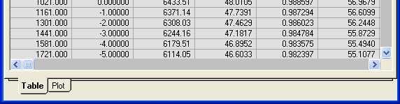
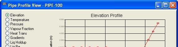
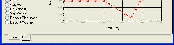
180 36 Two-Stage Compression Figure 20 Figure 21 Save your case! 36

181 Two-Stage Compression 37 Advanced Modeling Because the Recycle operation is a mathematical representation of a physical process, its location in a simulation is a particularly important one. The location of the tear stream can often determine success or failure to converge a recycle. Positioning the Recycle Operations for Optimum Performance When a user is deciding on a tear (Recycle) location, the first choice is often in the actual recycling stream. This is an acceptable choice if only one Recycle operation is being used. However, if more than one block is being used a better location may reduce the calculation time needed to solve the simulation. Careful choice of recycle position can also reduce the number of Recycle operations that are required. This will reduce the solution time and reduce the number of points at which an error can be introduced if the tolerance is too large. A very poor choice of a tear stream is a stream with an Adjust operation controlling one of its variables. Try to locate Recycles: To define multiple streams (i.e. before Tees, after Mixers). See Exercise 1. This means fewer recycle operations are needed. In streams with fixed conditions (i.e. cooler and heater outlets). This means fewer variables need to be iterated on. To avoid conflicts with Adjust operations. In major flow streams. These are likely to be more stable. Answers to the four subsequent Recycle Positioning Exercises are provided at the end of the module in the Answer Key section. 37

182 38 Two-Stage Compression Recycle Positioning Exercises Exercise 1 Examine the following PFD. This flowsheet has three physical recycles and three UniSim Design Recycle operations. What is the minimum number of recycle operations that are needed? Where should the recycle operation(s) be positioned? Figure 22 Exercise 1 38

183 Two-Stage Compression 39 Exercise 2 Assume the condenser outlet stream is fully defined (except flow rate), the chiller duty and outlet conditions are known, the pressure drops across the condenser and chiller are known, and the stage 1 compressor outlet pressure is known. This flowsheet is the refrigeration loop with economizer from Modules 2 and 3 of the UniSim Design 4526 course. How many recycles are needed in this flowsheet, where should they be placed, and why? Figure 23 Exercise 2 39

184 40 Two-Stage Compression Exercise 3 Assume that the feed stream (To Refrig) is fully defined, all pressure drops are known for the exchanger and the chiller as well as the LTS separator feed temperature. This flowsheet is the refrigerated gas plant from Module 3 of the UniSim Design 4526 course. How many recycles are needed in this flowsheet, where should they be placed, and why? Figure 24 Exercise 3 40

185 Two-Stage Compression 41 Exercise 4 Assume the Feed is completely defined. Also known are the shell and tube side pressure drops for E-100 and E-101, and the temperatures of streams 3 and 4. This flowsheet is really an extension of the PFD in Exercise 3. A column and overall material recycle have been appended to the gas plant flowsheet. N.B. that columns MUST have a fully specified feed stream to solve. (The only exception is that in UniSim Design R380.1 onwards pressure can be propagated from the column to the feed stream). How many recycles are needed in this flowsheet, where should they be placed, and why? Figure 25 Exercise 4 41

186 42 Two-Stage Compression Exercise 5: Compressor Curves As well as entering curves of head vs flow you can also enter pressure ratio vs flow. Another new feature means you can calculate the compressor design speed (use the Design Speed for this Compressor button on the Design tab Parameters page). This feature uses a correlation from the GPSA handbook. After finishing the simulation, your boss provides you with a set of Compressor Curves for the Stage 2 Compressor which now exists in the field. Will the existing Compressor be able to achieve the outlet pressure you want (i.e kpa), or will you have to add a third stage of compression? Flow, ACT [m3/min (ACFM)] Head [m (ft)] 30 (1000) 6000 (19670) (2000) 5950 (19500) (3400) 5800 (19000) (5000) 5500 (18000) (6200) 4800 (15700) (7300) 3360 (11000) 68 Polytropic Efficiency Challenge You complain to your boss that your simulation takes too long to converge on your computer because of the recycles and use this opportunity to petition for a new high speed computer. Your boss has a look at your simulation and denies your request on the basis that you can reduce your convergence time by eliminating one of the recycle unit operations in the simulation. Is your request justified or is your boss correct? 42

187 Two-Stage Compression 43 Answer Key Exercise 1 Examine the PFD above. This flowsheet has three physical recycles and three UniSim Design recycle operations. What is the minimum number of recycle operations that are needed? One. There are 3 separate loops and they overlap in stream 1. (Hint. Visualize the separate loops in the system. Which stream is included in all the loops?) Where should the recycle operation(s) be positioned? At the outlet of the mixer. Exercise 2 How many recycles are needed in this flowsheet, where should they be placed, and why? There is no need for a recycle operation in this refrigeration loop flowsheet due to the positioning of the specifications. Exercise 3 How many recycles are needed in this flowsheet, where should they be placed, and why? Again there is no need for a recycle operation. Since the LTS separator feed stream has a known temperature and pressure it is fully defined even though the Gas-Gas exchanger hasnt completely solved, hence the separator can solve and then the exchanger can solve. 43

188 44 Two-Stage Compression Exercise 4 How many recycles are needed in this flowsheet, where should they be placed, and why? There is no need for a recycle in the small loop containing the two exchangers and separator V-101 because the pressures and temperatures in streams 3 and 4 are known, hence stream 4 can flash fully before the exchangers are solved. However, the column will not be able to solve unless its feed stream is fully defined, hence a single recycle is needed somewhere in the main loop - for example in stream 1, 7 or 9. 44

189 Acid Gas Sweetening with DEA 1 Acid Gas Sweetening with DEA 2009 Honeywell All rights reserved. UniSim is a U.S. registered trademark of Honeywell International Inc R380.02

190 2 Acid Gas Sweetening with DEA 2

191 Acid Gas Sweetening with DEA 3 Workshop In this example, a typical acid gas treating facility is simulated. A water-saturated natural gas stream is fed to an amine contactor. For this example, Diethanolamine (DEA) at a strength of 28 wt% in water is used as the absorbing medium. The contactor consists of 20 real stages. The rich amine is flashed from the contactor pressure of 6900 kpa to 620 kpa before it enters the rich/lean amine exchanger, where it is heated to the regenerator feed temperature of 95 C. The regenerator also consists of 20 real stages. Acid gas is rejected from the regenerator at 50 C, while the lean amine is produced at approximately 110 C. The lean amine is cooled and recycled to the Contactor. Learning Objectives Once you have completed this section, you will be able to: Simulate Amine towers in UniSim Design Supply tray dimensions to calculate component efficiencies for Amine towers Use the Set operation Use the Spreadsheet Prerequisites Before beginning this section you need to be able to start a new case from scratch, add and contact streams and unit operations and be familiar with the column recycle operations. 3

192 4 Acid Gas Sweetening with DEA 4

193 Acid Gas Sweetening with DEA 5 Column Overview Contactor Figure 1 5

194 6 Acid Gas Sweetening with DEA Regenerator Figure 2 6

195 Acid Gas Sweetening with DEA 7 Building the Simulation Defining the Simulation Basis The Amine property package does not allow hypothetical components. For this case, you will be using the Amines property package with the following components: Nitrogen H2S CO2 Methane Ethane Propane i-butane n-butane i-pentane n-pentane n-hexane H2O DEAmine 1. Set up a new case, using the Amine Pkg property package with the components above. Use the Kent-Eisenberg and Non-Ideal Models. Amines Property Package The Amines package contains the thermodynamic models developed by D.B. Robinson & Associates for their proprietary amine plant simulator, AMSIM. Their equilibrium acid gas solubility and kinetic parameters for aqueous alkanolamine solutions in contact with H 2 S and CO 2 have been incorporated into this property package. The Amines property package has been fitted to extensive experimental data gathered from a combination of D.B. Robinsons in-house data, several unpublished sources and numerous technical references. For more information, refer to Appendix C of the Simulation Basis Manual. 7

196 8 Acid Gas Sweetening with DEA The Amines package incorporates a specialized stage efficiency model to permit the simulation of columns on a real tray basis. The stage efficiency model calculates H 2 S and CO 2 component stage efficiencies based on the tray dimensions and the calculated internal tower conditions for both absorbers and strippers. Adding the Basics Adding the feed streams 2. Add a new stream for the inlet gas with the following values: In this cell... Enter... Name Sour Gas Temperature 25 C (75 F) Pressure 6900 kpa (1000 psia) Molar Flow 1250 kgmole/h (25 MMSCFD) Component Mole Fraction Nitrogen H2S CO Methane Ethane Propane i-butane n-butane i-pentane n-pentane n-hexane H2O DEAmine 0.0 8

197 Acid Gas Sweetening with DEA 9 3. Add a second stream for the lean amine feed to the amine contactor with the following values: Make sure you enter the DEAmine and H2O compositions on a weight (mass) basis. In this cell... Enter... Name DEA to Contactor Temperature 35 C (95 F) Pressure 6850 kpa (995 psia) Std Ideal Liq Vol Flow 43 m3/h (190 USGPM) Component Mass Fraction H2O 0.72 DEAmine 0.28 The values for the stream DEA to Contactor will be updated once the recycle operation is installed and has calculated. Adding the Physical Unit Operations Separator Operation Any free water carried with the gas is first removed in a Separator operation, FWKO TK. 4. Add a Separator and provide the following information: In this cell... Connections Name Inlet Vapour Outlet Liquid Outlet Enter... FWKO TK Sour Gas Gas to Contactor FWKO What is the flow rate of water in FWKO? 9

198 10 Acid Gas Sweetening with DEA Contactor Operation The amine contactor is simulated using an Absorber operation in UniSim Design. 5. Add an Absorber column operation with the following specifications: In this cell... Enter... Connections Name DEA Contactor No. of Stages 20 Top Stage Inlet DEA to Contactor Bottom Stage Inlet Gas to Contactor Ovhd Vapour Outlet Sweet Gas Bottoms Liquid Outlet Rich DEA Pressures Top 6850 kpa (995 psia) Bottom 6900 kpa (1000 psia) Estimates Top Temperature 40 C (100 F) Bottom Temperature 70 C (160 F) The Amines property package requires that real trays be used in the contactor and regenerator operations. To model this, in UniSim Design, component specific efficiencies are required for H 2 S and CO 2 on a tray by tray basis. These proprietary efficiency calculations are provided in the column as part of the Amines package. Tray dimensions must be supplied to enable this feature. Tray dimensions enable component specific efficiencies to be calculated by estimating height of liquid on the tray and the residence time of vapour in the liquid. To supply the dimensions for Amines calculations, switch to the Parameters tab, Amines page. 6. Enter the dimensions shown in the figure below. The dimensions in field units are given in the table on the left. 10

199 Acid Gas Sweetening with DEA 11 Figure 3 7. Run the Column. 8. Once the Column has converged, move to the Efficiencies page on the Parameters tab. 9. Select the Component radio button in the Efficiency Type group to view the component efficiencies. Figure Switch to the Worksheet tab to view the concentrations of H 2 S and CO 2 in the product streams from the column. 11

200 12 Acid Gas Sweetening with DEA What is the concentration of H2S and CO2 in the Sweet Gas? H2S CO2 Valve Operation Rich DEA from the Contactor is directed to a Valve, VLV-100, where the pressure is reduced to 620 kpa (90 psia), which is close to the Regenerator operating pressure. 11. Add a Valve with the following values: In this cell... Connections Inlet Outlet Worksheet Pressure, DEA to Flash TK Enter... Rich DEA DEA to Flash TK 620 kpa (90 psia) Separator Operation Gases which are flashed off from Rich DEA are removed using the rich amine flash tank, Flash TK, which is installed as a Separator operation. 12. Add a Separator with the information shown below: In this cell... Connections Name Inlets Vapour Outlet Liquid Outlet Enter... Flash TK DEA to Flash TK Flash Vap Rich to L/R 12

201 Acid Gas Sweetening with DEA 13 Heat Exchanger Operation Regen Feed is heated to 95 C (200 F) in the lean/rich exchanger, L/R HEX, prior to entering the Regenerator, where heat is applied to break the amine-acid gas bonds, thereby permitting the DEA to be recycled to the contactor. 13. Add a Heat Exchanger with the following values: In this cell... Connections Name Tube Side Inlet Tube Side Outlet Shell Side Inlet Shell Side Outlet Parameters Tubeside Delta P Shellside Delta P Heat Exchanger Model Worksheet Regen Feed, Temperature Enter... L/R HEX Rich to L/R Regen Feed Regen Bttms Lean from L/R 70 kpa (10 psi) 70 kpa (10 psi) Exchanger Design (Weighted) 95 C (203 F) Regenerator Operation Damping Factors will have no effect on problems where the heat and spec error does not converge. Certain columns require the use of a damping factor. Amine Regenerators, TEG Strippers and Sour Water Strippers use damping factors in the range. The Amine Regenerator is modeled as a Distillation Column. There are 20 real stages - 18 stages in the Tray Section plus a Reboiler and Condenser. The component efficiencies for this tower are assumed to be constant at 0.8 for H 2 S and 0.15 for CO 2. The efficiencies of the Condenser and Reboiler must remain at 1.0, so only stages 1-18 should have efficiencies entered for them. A Damping Factor of 0.4 will provide a faster, more stable convergence. The Damping Factor controls the step size used in the outer loop when updating the thermodynamic models in the inner loop. 13

202 14 Acid Gas Sweetening with DEA 14. Add a Distillation column with the following information: The Input Experts are toggled on and off from the Simulation tab of the Preferences view. Condenser and Reboiler temperature specifications are added as Column Temperature specifications; dont forget to activate them. An alternative specification that could be used is the Component Recovery for DEA. All of the DEA (100%) should be recovered in the bottom product stream. In this cell... Connections Name No. of Stages 18 Enter... Regenerator Feed Streams / Stage Regen Feed / 4 Condenser Type Ovhd Vapour Outlet Bottoms Liquid Outlet Reboiler Energy Stream Condenser Energy Stream Parameters/Solver Full Reflux Acid Gas Regen Bttms Rblr Q Cond Q Fixed Damping Factor 0.40 Solving Method Profiles Condenser Pressure Condenser Delta P Reboiler Pressure Top Stage Temperature Reboiler Temperature Efficiencies CO H2S 0.8 Monitor Overhead Rate (Estimate) Reflux Ratio (Estimate) Specs Column Temperature, Condenser Column Duty, Reboiler 15. Run the column. Legacy Inside-Out 190 kpa (27.5 psia) 15 kpa (2.5 psi) 220 kpa (31.5 psia) 100 C (210 F) 125 C (260 F) 75 kgmole/h (1.5 MMSCFD) C (120 F) 1.3e7 kj/h (1.2e7 Btu/hr) 14

203 Acid Gas Sweetening with DEA 15 Mixer Operation Water make-up is necessary, since water will be lost in the Absorber and Regenerator overhead streams. A Mixer operation combines the lean amine from the Regenerator with a water makeup. These streams mix at the same pressure. The Mixer will adjust the water flow rate to achieve the circulation rate. An Adjust operation could have been used but is not necessary. 16. Add a new stream. In this cell... Enter... Connections Name Makeup H2O Temperature 25 C (77 F) Component Mole Fraction H2O Add a Mixer with the following information: In this cell... Connections Inlets Outlet Parameters Pressure Assignment Worksheet Std Ideal Liq Vol Flow, DEA to Cool Enter... Makeup H2O Lean from L/R DEA to Cool Equalize All 43 m3/h (190 USGPM) What is the flow rate of Makeup H2O? 15

204 16 Acid Gas Sweetening with DEA Cooler Operation 18. Add a Cooler with the values given below: In this cell... Connections Name Feed Stream Product Stream Energy Stream Parameters Pressure Drop Enter... Cooler DEA to Cool DEA to Pump Cooler Q 35 kpa (5 psi) Pump Operation 19. Add a Pump with the following information: In this cell... Connections Inlet Outlet Energy Worksheet Temperature, DEA to Recycle Enter... DEA to Pump DEA to Recycle Pump Q 35 C (95 F) 16

205 Acid Gas Sweetening with DEA 17 Adding Logical Unit Operations Set Operation Set icon The Set is a steady-state operation used to set the value of a specific Process Variable (PV) in relation to another PV. The relationship is between the same PV in two like objects; for instance, the temperature of two streams, or the UA of two exchangers. 20. Double-click on the Set icon. Complete the Connections tab as shown in the following figure. Figure Go to the Parameters tab. Set the Multiplier to 1, and the Offset to -35 kpa (-5 psi) as shown below: 17

206 18 Acid Gas Sweetening with DEA Figure 6 Recycle Operation Recycle icon The Recycle installs a theoretical block in the process stream. The feed into the block is termed the calculated recycle stream, and the product is the assumed recycle stream. The following steps take place during the convergence process: UniSim Design uses the conditions of the assumed stream and solves the Flowsheet up to the calculated stream. UniSim Design then compares the values of the calculated stream to those of the assumed stream. Based on the difference between the values, UniSim Design modifies the values in the assumed stream. The calculation process repeats until the values in the calculated stream match those in the assumed stream within specified tolerances. In this case, the lean amine (DEA to Contactor) stream which was originally estimated will be replaced with the new calculated lean amine (DEA to Recycle) stream and the Contactor and Regenerator will be run until the recycle loop converges. 22. Double-click on the Recycle icon. On the Connections tab select the connections from the drop-down lists as follows: 18

207 Acid Gas Sweetening with DEA 19 Figure Switch to the Parameters tab. Ensure the tab is as shown in the figure below: Figure 8 The smaller the Sensitivity the tighter the tolerance. Save your case! 19

208 20 Acid Gas Sweetening with DEA Analyzing the Results The incoming sour gas contained 4.1% CO 2 and 1.7% H 2 S. For our inlet gas flow rate of 1250 kgmole/h (25 MMSCFD), a circulating solution of approximately 28 wt% DEA was used to remove H 2 S and CO 2. The conventional pipeline gas specification is no more than 2.0 vol% CO 2 and 4 ppm (volume) H 2 S. To calculate vol ppm multiply liquid volume fraction by 1 million. What is the C02 vol% in the Sweet Gas? What is the H2S vol ppm level? Have the specifications been met? 20

209 Acid Gas Sweetening with DEA 21 Advanced Modeling Concentrations of acid gas components in an amine stream are typically expressed in terms of loadings of amine. Loadings are defined as moles of the particular acid gas divided by moles of the circulating amine. The Spreadsheet in UniSim Design is well-suited for this calculation. Not only can the loadings be directly calculated and displayed, but they can be incorporated into the simulation to provide a control point for optimizing the amine simulation. 24. Add a spreadsheet using the following variables for the loading calculations: Figure 9 The following formulas will produce the desired calculations: 21

210 22 Acid Gas Sweetening with DEA Figure 10 The acid gas loadings can be compared to values recommended by D.B. Robinson. Maximum Acid Gas Loadings (moles acid gas / moles of amines) CO2 H2S MEA, DEA DEA TEA, MDEA Figure 11 22

211 Acid Gas Sweetening with DEA 23 Exploring the Simulation Exercise 1: Doubling the Flow rate You just received a phone call from the plant manager at a neighboring gas plant. They are having a problem with their contactor and must shut down. You have agreed to take on their gas for processing, which doubles the flow rate of gas to your plant. Make the necessary changes to handle the upset. 23

212 24 Acid Gas Sweetening with DEA 24

213 Natural Gas Dehydration with TEG 1 Natural Gas Dehydration with TEG 2009 Honeywell All rights reserved. UniSim is a U.S. registered trademark of Honeywell International Inc R380.02

214 2 Natural Gas Dehydration with TEG 2

215 Natural Gas Dehydration with TEG 3 Workshop At the wellhead, reservoir fluids generally are saturated with water. The water in the gas can present some problems: formation of solid hydrates can plug valves, fittings, or pipes the presence of water along with H2S or CO2 can cause corrosion problems water can condense in the pipeline causing erosion or corrosion problems Generally, a dehydration unit is used in gas plants to meet a pipeline specification. There are several different processes available for dehydration: glycols, silica gel, or molecular sieves. The natural gas industry commonly uses tri-ethylene glycol (TEG) for gas dehydration where low gas dew point temperatures are required, such as in the design of offshore platforms in the Arctic or North Sea regions or for other cryogenic processes. In this example, the water dew point spec for the dry gas is -10 C (-14 F) at 6155 kpa (893 psia). Learning Objectives Once you have completed this section, you will be able to: Model a typical TEG dehydration unit Determine water dew point for a gas Prerequisites Before beginning this section you need to be able to add streams, operations and columns. 3

216 4 Natural Gas Dehydration with TEG 4

217 Natural Gas Dehydration with TEG 5 Column Overview TEG Contactor Figure 1 TEG Regenerator Figure 2 5

218 6 Natural Gas Dehydration with TEG Building the Simulation Defining the Simulation Basis For this case, you will be using the Peng-Robinson EOS with the following components: Nitrogen H2S CO2 Methane Ethane Propane i-butane n-butane i-pentane n-pentane H2O TEGlycol 1. Set up a new case, using the Peng-Robinson property package with the components above. Starting the Simulation Adding the feed streams 2. Add a Material stream for the inlet gas with the following values: In this cell... Enter... Name Inlet Gas Temperature 30 C (85 F) Pressure 6200 kpa (900 psia) Molar Flow 500 kgmole/h (10 MMSCFD) Component Mole Fraction Nitrogen H2S

219 Natural Gas Dehydration with TEG 7 In this cell... Enter... CO Methane Ethane Propane i-butane n-butane i-pentane n-pentane H2O TEGlycol Add a second Material stream for the TEG feed to the TEG Contactor with the listed values. Dont forget to enter these compositions as mass fractions! In this cell... Enter... Name TEG Feed Temperature 50 C (120 F) Pressure 6200 kpa (900 psia) Std Ideal Liq Vol Flow 0.5 m3/h (2 USGPM) Component Mass Fraction H2O 0.01 TEGlycol 0.99 The values for the stream TEG Feed will be updated once the Recycle operation is installed and has calculated. Mixer Operation The composition of the natural gas stream has been provided on a water-free basis. To ensure water saturation, the gas is mixed with water prior to entering the Contactor. 4. Add a Mixer to mix the Inlet Gas and Water to Saturate streams. 7

220 8 Natural Gas Dehydration with TEG In this cell... Connections Name Inlets Outlet Parameters Automatic Pressure Assignment Worksheet Water to Saturate, Flow rate Water to Saturate, Composition Water to Saturate, Temperature Enter... Saturate Inlet Gas Water to Saturate Gas + H2O Equalize All 0.5 kgmole/h (1.1 lbmole/hr) 100% Water 30 C (85 F) What is the vapour fraction of the stream Gas+H20? (It should be less than 1.0 to ensure saturation) Separator Operation Any free water carried with the gas is first removed in a separator operation, FWKO. 5. Add a Separator and provide the following information: In this cell... Connections Name Inlets Vapour Outlet Liquid Outlet Enter... FWKO TK Gas + H2O Gas to Contactor FWKO 8

221 Natural Gas Dehydration with TEG 9 How much water is removed by the Separator? What is the hydrate temperature of Gas to Contactor? Contactor Operation The TEG Contactor can now be simulated. 6. Add an Absorber column operation with the following specifications and Run the column. In this cell... Enter... Connections Name TEG Contactor No. of Stages 8 Top Stage Inlet TEG Feed Bottom Stage Inlet Gas to Contactor Ovhd Vapour Outlet Dry Gas Bottoms Liquid Outlet Rich TEG Pressure Top 6190 kpa (897 psia) Bottom 6200 kpa (900 psia) Valve Operation The Rich TEG stream is flashed across the valve, VLV-100. The outlet pressure will be back calculated. 7. Add a Valve with the following values: In this cell... Connections Inlet Outlet Enter... Rich TEG LP TEG 9

222 10 Natural Gas Dehydration with TEG Heat Exchanger Operation Regen Feed is heated to 105 C (220 F) in the lean/rich exchanger, L/R HEX, before entering the Regenerator. 8. Add a Heat Exchanger with the following values: In this cell... Connections Name Tube Side Inlet Tube Side Outlet Shell Side Inlet Shell Side Outlet Parameters Tubeside Delta P Shellside Delta P Worksheet Regen Feed, Temperature Regen Feed, Pressure Enter... L/R HEX Regen Bttms Lean from L/R LP TEG Regen Feed 70 kpa (10 psi) 70 kpa (10 psi) 105 C (220 F) 110 kpa (16 psia) Regenerator Operation The TEG Regenerator is simulated as a Distillation Column. The TEG Regenerator consists of a condenser, a reboiler and one ideal stage. 9. Add a Distillation Column to the case. You can turn off the Column Input Experts in Tool/Preferences on the Simulation tab by un-checking the Use Input Experts box. In this cell... Enter... Connections Name TEG Regenerator No. of Stages 1 Inlet Stream Regen Feed Condenser Type Full Reflux Ovhd Vapour Outlet Sour Gas Bottoms Liquid Outlet Regen Bttms Condenser Energy Stream Cond Q Reboiler Energy Stream Reb Q 10

223 Natural Gas Dehydration with TEG 11 In this cell... Enter... Pressures Delta P Cond 2 kpa (1 psia) Condenser 101 kpa (14 psia) Reboiler 103 kpa (15 psia) Specs First Spec - Column Temperature Stage Condenser Spec Value 102 C (215 F) Status Active Second Spec - Column Temperature Stage Reboiler Spec Value 205 C (400 F) Status Active Third Spec - Reflux Ratio Spec Value 1.0 Molar Status Estimate Fourth Spec - Column Draw Rate Draw Sour COL2 Spec Value 1 kgmole/h (0.02 MMSCFD) Status Estimate 10. Set the Damping method (on the Solver page of the Parameters tab) to Adaptive. This will result in much faster convergence for this column. 11. Run the Column. Mixer Operation TEG is lost in small quantities in the top products of the columns, so a makeup stream is required to ensure that the material balance is maintained. 12. Add a Material Stream with the following information: 11

224 12 Natural Gas Dehydration with TEG Dont forget to enter the compositions as mass fractions! In this cell... Enter... Connections Name Makeup TEG Temperature 15 C (60 F) Component Mass Fraction H2O 0.01 TEG Add a Mixer with the following information: In this cell... Connections Inlets Outlet Parameters Automatic Pressure Assignment Worksheet Std Ideal Liq Vol Flow, TEG to Pump Enter... Makeup TEG Lean from L/R TEG to Pump Equalize All 0.5 m3/h (2 USGPM) What is the flow rate of Makeup TEG? Pump Operation A pump is installed to raise the pressure of the TEG before it enters the Contactor. 14. Add a Pump with the following information: 12

225 Natural Gas Dehydration with TEG 13 In this cell... Connections Inlet Outlet Energy Worksheet Pump Out, Pressure Enter... TEG to Pump Pump Out Pump Q 6275 kpa (910 psia) Heat Exchanger A second heat exchanger is added to cool the TEG returning to the Contactor. 15. Add a Heat Exchanger with the following information: In this cell... Connections Tube Side Inlet Tube Side Outlet Shell Side Inlet Shell Side Outlet Parameters Tube Side Delta P Shell Side Delta P Worksheet TEG to Recycle, Temperature Enter... Pump Out TEG to Recycle Dry Gas Sales Gas 70 kpa (10 psi) 35 kpa (5 psi) 50 C (120 F) Recycle Operation Recycle icon The Recycle installs a theoretical block in the process stream. The feed into the block is termed the calculated recycle stream, and the product is the assumed recycle stream. The following steps take place during the convergence process: UniSim Design uses the conditions of the assumed stream and solves the Flowsheet up to the calculated stream UniSim Design then compares the values of the calculated stream to those of the assumed stream 13

226 14 Natural Gas Dehydration with TEG Based on the difference between the values, UniSim Design modifies the values in the assumed stream The calculation process repeats until the values in the calculated stream match those in the assumed stream within specified tolerances The specifications in the lean TEG (TEG Feed) stream which were originally estimated will be replaced by values updated by the recycle. The recycle will control iterations of the loop until it converges. 16. Double-click the Recycle icon from the Object Palette. On the Connections tab select the connections from the drop-down boxes as depicted below: Figure 3 The TEG concentration is very high so it is necessary to tighten the tolerances, especially for composition, to ensure an accurate solution. 17. Switch to the Variables page on the Parameters tab. Complete the page as shown in the figure below. Tolerances for Flow, Enthalpy and Composition need to be tightened. 14

227 Natural Gas Dehydration with TEG 15 Figure 4 Hydrate Formation Utility There are three ways to attach utilities to streams. Click on the Tools menu and select Utilities. The Available Utilities view appears Press Ctrl U and the Available Utilities view appears Double-click a stream. On the Attachments tab, select Utilities. Click Create and the Available Utilities view appears Attach a Hydrate Formation Utility to Stream Sales Gas 18. Press Ctrl U and in the Available Utilities view, select the Hydrate Formation Utility and click on the Add Utility button. If the utility is not already associated with a stream, then the Hydrate Formation Utility view appears. 19. Click Select Stream and select the Sales Gas. Click OK. 20. Switch to the Performance tab. Here you will see the Equilibrium Phase reported as Vapour Phase. 15

228 16 Natural Gas Dehydration with TEG Figure 5 What is the hydrate temperature of the Sales Gas stream? How does this compare with the hydrate temperature of the Gas to Contactor stream? Save your case! Analyzing the Results Component Splitter icon One of the criteria used to determine the efficiency of a dehydration facility is the water dew point of the dry gas. First, all traces of TEG must be removed from the stream being tested because TEG affects the water dew point. This is accomplished by the use of a Component Splitter and a property correlation to calculate the water dew point temperature. 16

229 Natural Gas Dehydration with TEG Add a Component Splitter with the following values: The Component Splitter does not do a flash to separate components. The separation is specified by the user. In this cell... Connections Name Inlet Overhead Outlet Bottoms Outlet Energy Parameters TEG Only, Temperature Water Dew Point, Temperature Stream Specifications Splits Enter... Remove TEG Sales Gas TEG Only Water Dew point Split Q 35 C (95 F) 35 C (95 F) Equalize All Stream Pressures Stream TEG Only, TEG 1.0 Stream TEG Only, all other components 0.0 The next step is to add a Water Dew Point Property Correlation to the Water Dew Point stream. 22. Double-click on the Water Dew Point stream. 23. Open the Properties page on the Worksheet tab. The property correlations displayed are controlled using the buttons at the bottom of the Properties page. Figure 6 Append New Correlation icon 24. Click the Append New Correlation button. The Correlation Picker view appears displaying all the available correlations in a tree format. 25. From the list of available correlations click on the + symbol to view additional sub-items for the Gas branch. Select the Water Dew Point correlation (see Figure 7) and click Apply. Close the Correlation Picker. The new correlation is added to the bottom of the list. 17

230 18 Natural Gas Dehydration with TEG Figure Locate the Water Dew Point [Gas] property correlation that was just added. Figure 8 What is the water dew point temperature of the Sales Gas stream? Does it meet the required spec: -10 C (-14 F) at 6155 kpa (893 psia)? 18

231 Natural Gas Dehydration with TEG 19 Exploring the Simulation Exercise 1: Stripping Gas The addition of stripping gas (slip stream from Sales Gas) will enhance the ability of the Regenerator to remove water from the rich TEG. Take note of the current concentration of TEG in the Regen Bttms stream. 1. Add a Tee operation to split the Sales Gas into two streams. The strip gas stream is specified as follows: Flow = 50 kgmole/h (110 lbmole/hr) The stream pressure is 6155 kpa which is too high for the Regenerator. 2. Add a valve and heater to prepare the Strip Gas stream to be a feed to the Regenerator. Specify the following parameters for the heater: Delta P = 50 kpa Product stream name = SG to Regen 3. Specify the following parameters for stream SG to Regen: T = 70 C (160 F) P = 110 kpa (15 psia) 4. Connect stream SG to Regen as a feed to the Regenerator Reboiler. Does the TEG concentration in Regen Bttms increase? Note: the sales gas now exceeds the dew point specification easily. 19

232 20 Natural Gas Dehydration with TEG 20

233 Reporting in UniSim Design 1 Reporting in UniSim Design 2008 Honeywell All rights reserved. UniSim is a U.S. registered trademark of Honeywell International Inc R380.01

234 2 Reporting in UniSim Design 2

235 Reporting in UniSim Design 3 Introduction Once you have finished a simulation, or during analysis, you may wish to obtain reports of the data that you have input and that UniSim Design has generated. Reporting data in UniSim Design can be achieved in a number of ways, such as: Report manager Print to File option Copy-Paste with Labels option Workbook and PFD customization Excel utilities Learning Objectives Once you have finished this module, you will be able to customize reports in UniSim Design using the Report Manager, customize the PFD and the workbook to display selected data and install and run an Excel utility to view data from the workbook. Prerequisites Familiarity with the UniSim Design interface Ability to modify the workbook in UniSim Design Knowledge of Microsoft Excel 3

236 4 Reporting in UniSim Design Report Manager The Report Manager in UniSim Design allows the user to include data from all unit operations and streams in a UniSim Design case in any order. This information can then be printed. The information available through the Report Manager is the same information available if one prints a unit operation or stream report directly from the UniSim Design case. Exercise 1 1. Open the solution case from the Gas Dehydration with TEG module, NGDehydrationTEG.usc, found on the disk with your training materials. Information about operations and streams in UniSim Design used for printing is contained in objects called Datasheets. 2. Go to the Tools menu, and select Reports. You are now in the Report Manager. 3. Click the Create button to create a new report. You are presented with a new window that allows you to customize the content of the report. 4. Click the Insert Datasheet button to obtain a menu of all the information available in the case that can be included in the report: Figure 1 5. You can filter the lists by object type or by name, using the radio buttons at the top of the window. In this case, leave the radio button on Pick a Specific Object by Name. 4

237 Reporting in UniSim Design 5 6. Leave the Flowsheets selection at Case (Main) and choose stream Sales Gas under the Objects list. You will notice that all the datablocks available for stream Sales Gas have been selected by default in the Available Datablocks window: Figure 2 7. The only information we want to include in our datasheet is the stream conditions, so you need to click on the + next to the Worksheet option and deselect all the remaining selections (e.g. Properties, Composition and K values). You will also need to deselect Attachments, Dynamics, User Variables and Notes: Figure 3 8. Click the Add button to add the Conditions for stream Sour Gas to the report. You will notice that the report now contains the conditions for stream Sales Gas. 9. Now, add the Regenerator column Design Datablock to the report in the same way. (HINT: the Flowsheets selection must be left at Case(Main) in order to select the Design Datablock for a column.) 5

238 6 Reporting in UniSim Design 10. In the report manager, you can add information from the workbook as well as from streams and Unit operations. Add the Unit Operations page from the Main flowsheet workbook to the report. 11. We are now finished adding datasheets to the report. Close the Select Datablocks for Datasheet window. 12. On the Report Manager window, you can see that you can change the order in which the datasheets are presented in the report, and you can edit the content as well. In addition, you can change the name of the report. Change the name of this report to Dehy Report. Figure You can also change the format and layout of the report, as well as the unit set used in the report. Click on the Format/Layout button and select the Field Unit Set. This unit set will now always be associated with this report. Close the window. 14. You are now ready to Print or Preview the report. In this case, we will not print the report to paper, but we will preview it. Click the Preview button to see what the report would look like when printed. Note that user specified values are identified on the printout with an asterisk, *,next to them. Save your case! 6