Fraser River Sockeye Production Dynamics

Transcription

1 February 2011 technical report 10 Fraser River Sockeye Production Dynamics Randall M. Peterman and Brigitte Dorner The Cohen Commission of Inquiry into the Decline of Sockeye Salmon in the Fraser River

2 Fraser River Sockeye Production Dynamics Randall M. Peterman 1 and Brigitte Dorner 2 1 School of Resource and Environmental Management, Simon Fraser University, 8888 University Drive, Burnaby, BC V5A 1S6 2 Driftwood Cove Designs, GD Lasqueti Island, BC V0R 2J0 Technical Report 10 February 2011 Recommended citation for this report: Peterman, R.M. and B. Dorner Fraser River sockeye production dynamics. Cohen Commission Tech. Rept. 10: 133p. Vancouver, B.C.

3 Preface Fraser River sockeye salmon are vitally important for Canadians. Aboriginal and non-aboriginal communities depend on sockeye for their food, social, and ceremonial purposes; recreational pursuits; and livelihood needs. They are key components of freshwater and marine aquatic ecosystems. Events over the past century have shown that the Fraser sockeye resource is fragile and vulnerable to human impacts such as rock slides, industrial activities, climatic change, fisheries policies and fishing. Fraser sockeye are also subject to natural environmental variations and population cycles that strongly influence survival and production. In 2009, the decline of sockeye salmon stocks in the Fraser River in British Columbia led to the closure of the fishery for the third consecutive year, despite favourable pre-season estimates of the number of sockeye salmon expected to return to the river. The 2009 return marked a steady decline that could be traced back two decades. In November 2009, the Governor General in Council appointed Justice Bruce Cohen as a Commissioner under Part I of the Inquiries Act to investigate this decline of sockeye salmon in the Fraser River. Although the two-decade decline in Fraser sockeye stocks has been steady and profound, in 2010 Fraser sockeye experienced an extraordinary rebound, demonstrating their capacity to produce at historic levels. The extreme year-to-year variability in Fraser sockeye returns bears directly on the scientific work of the Commission. The scientific research work of the inquiry will inform the Commissioner of the role of relevant fisheries and ecosystem factors in the Fraser sockeye decline. Twelve scientific projects were undertaken, including: Project 1 Diseases and parasites 2 Effects of contaminants on Fraser River sockeye salmon 3 Fraser River freshwater ecology and status of sockeye Conservation Units 4 Marine ecology 5 Impacts of salmon farms on Fraser River sockeye salmon 6 Data synthesis and cumulative impact analysis 7 Fraser River sockeye fisheries harvesting and fisheries management 8 Effects of predators on Fraser River sockeye salmon 9 Effects of climate change on Fraser River sockeye salmon 10 Fraser River sockeye production dynamics 11 Fraser River sockeye salmon status of DFO science and management 12 Sockeye habitat analysis in the Lower Fraser River and the Strait of Georgia Experts were engaged to undertake the projects and to analyse the contribution of their topic area to the decline in Fraser sockeye production. The researchers draft reports were peer-reviewed and were finalized in early Reviewer comments are appended to the present report, one of the reports in the Cohen Commission Technical Report Series.

4 1 Executive summary Our main objective in this report is to present data and analyses that will contribute to the understanding of possible causes of reduced abundance and productivity of Fraser River sockeye salmon. We hope that our data, as well as analyses by other scientists who use them, will help to gain a better understanding of the causes of the dramatic changes in Fraser River sockeye salmon and thereby aid in developing appropriate management responses. Here, "productivity" is the number of adult returns produced per spawner, where "spawners" are the fish that reproduce for a given sockeye population in a given year, and "adult returns" (or recruits ) refer to the number of mature adult salmon resulting from that spawning that return to the coast prior to the onset of fishing. To achieve our objective, we obtained data sets on abundance of spawners and their resulting adult returns for a total of 64 populations ("stocks") of sockeye salmon. These stocks included 19 from the Fraser River, with the rest from other parts of British Columbia, Washington state, and Alaska. Almost all of our data are from wild populations that are not confounded by hatchery stocking. Data sets were of varying length, some starting as early as We included data on sockeye populations outside of the Fraser River to determine whether the Fraser's situation is unique, or whether other sockeye populations are suffering the same fate. In addition to obtaining data on adults, we also obtained data on juvenile (i.e., fry or smolt) abundance in fresh water for 24 sockeye populations to help determine whether problems leading to the long-term decline survival arose mainly in fresh water or the ocean. Unfortunately, we were not able to include any 2010 salmon data because the responsible agencies are still processing field samples to determine what portion of the fish belong to which particular stocks. We used three different measures of productivity: (1) number of adult returns per spawner, (2) an index that accounts for the influence of spawner abundance on returns per spawner and thus specifically represents productivity changes that are attributable to causes other than spawner abundance (e.g., environmental factors), and (3) an extension of the second index that uses a Kalman filter to remove high-frequency year-to-year variation ("noise") in productivity and thereby brings out the long-term trends that are of primary interest to sockeye managers. We compared time trends in these three productivity estimates across sockeye stocks within the Fraser River and among them and non-fraser sockeye stocks using a variety of methods, including visual comparisons, correlation analysis, Principal Components Analysis, and clustering.

5 We found that most Fraser and many non-fraser sockeye stocks, both in Canada and the U.S.A., show a decrease in productivity, especially over the last decade, and often also over a period of decline starting in the late 1980s or early 1990s. Thus, declines since the late 1980s have occurred over a much larger area than just the Fraser River system and are not unique to it. This observation that productivity has followed shared trends over a much larger area than just the Fraser River system is a very important new finding. More specifically, there have been relatively large, rapid, and consistent decreases in sockeye productivity since the late 1990s in many areas along the west coast of North America, including the following stocks (from south to north). 2 Puget Sound (Lake Washington) Fraser River Barkley Sound on the West Coast of Vancouver Island (Great Central and Sproat Lakes) Central Coast of B.C. (Long Lake, Owikeno Lake, South Atnarko Lakes) North Coast of B.C. (Nass and Skeena) Southeast Alaska (McDonald, Redoubt, Chilkat). Yakutat (northern part of Southeast Alaska) (East Alsek, Klukshu, Italio). The time trends in productivity for these stocks are not identical, but they are similar. This feature of shared variation in productivity across multiple salmon populations is consistent with, but may have occured over a larger spatial extent than, previously published results for sockeye salmon. In contrast, western Alaskan sockeye populations have generally increased in productivity over the same period, rather than decreased. Historical data on survival rates of Fraser sockeye stocks by life stage show that declines in total-life-cycle productivity from spawners to recruits have usually been associated with declines in juvenile-to-adult survival, but not the freshwater stage of spawner-to-juvenile productivity. Specifically, for the nine Fraser sockeye stocks with data on juvenile abundance (fry or seawardmigrating smolts), only the Gates stock showed a long-term reduction over time in freshwater productivity (i.e., from spawners to juveniles) concurrent with the entire set of years of its declining total life-cycle productivity from spawners to recruits. In contrast, seven of the nine stocks (excluding Late Shuswap and Cultus) showed reductions in post-juvenile productivity (i.e., from juveniles to returning adult recruits) over those years with declining productivity from spawners to recruits. These results indicate either that the primary mortality agents causing the decline in Fraser River sockeye occurred in the post-juvenile stage (marine and/or late fresh

6 water), or that certain stressors (such as pathogens) that were non-lethal in fresh water caused mortality later in the sockeye life history. The large spatial extent of similarities in productivity patterns that we found across populations suggests that there might be a shared causal mechanism across that large area. Instead, it is also possible that the prevalence of downward trends in productivity across sockeye stocks from Lake Washington, British Columbia, Southeast Alaska, and the Yakutat region of Alaska is entirely or primarily caused by a coincidental combination of processes such as freshwater habitat degradation, contaminants, pathogens, predators, etc., that have each independently affected individual stocks or smaller groups of stocks. However, the fact that declines also occurred outside the Fraser suggests that mechanisms that operate on larger, regional spatial scales, and/or in places where a large number of correlated sockeye stocks overlap, should be seriously examined in other studies, such as the ones being done by the other contractors to the Cohen Commission. Examples of such large-scale phenomena affecting freshwater and/or marine survival of sockeye salmon might include (but are not limited to) increases in predation due to various causes, climate-driven increases in pathogen-induced mortality, or reduced food availability due to oceanographic changes. Further research is required to draw definitive conclusions about the relative influence of such large-scale versus more local processes. The Harrison River sockeye stock in the Fraser River watershed is an important exception to the decreasing time trends in productivity that have been widely shared across sockeye stocks. Harrison fish have notable differences in their life history strategy from the majority of other sockeye populations that we examined, including other Fraser River stocks. These life history differences may provide an important clue about causes of the decline in other sockeye stocks. Specifically, (1) Harrison fish migrate to sea in their first year of life as fry instead of overwintering in fresh water and migrating to sea in their second year as smolts, (2) they appear to rear for some time in the Fraser River estuary, (3) they remain in the Strait of Georgia later than other Fraser River sockeye, and (4) there is some evidence that the fry migrate out around the southern end of Vancouver Island through the Strait of Juan de Fuca instead of through Johnstone Strait to the north. That southern fry-migration route is shared with Lake Washington sockeye, yet the latter stock was one of those that showed a decrease in productivity similar to that of other B.C. sockeye stocks. Thus, the reason for the Harrison's exceptional trend is probably not attributable simply to its different migration route. We hope that by using our data on productivity trends for Harrison and other stocks, the other contractors to the Cohen Commission will find an explanation for why the Harrison situation is anomalous. In addition to describing similarities in productivity patterns, we also evaluated the hypothesis that large numbers of spawners could be detrimental to productivity (recruits per spawner) of Fraser sockeye populations. The downward time trend in productivity of these 3

7 stocks, combined with successful management actions to rebuild spawner abundances, has led to speculation that these unusually large spawner abundances might in fact be to blame for declines in productivity and consequently also substantial declines in returns. For the Quesnel sockeye stock on the Fraser, there is indeed evidence that interactions between successive brood lines that are associated with large spawner abundances may have reduced productivity of subsequent cohorts. Thus, the recent decline in productivity for Quesnel sockeye might be more attributable to increased spawner abundance than to broad-scale environmental factors that affect other sockeye stocks in the Fraser and other regions. However, other Fraser sockeye populations do not show such evidence. Our data do not support the hypothesis that large spawner abundances are responsible for widespread declines. 4 Recommendations We conclude with five recommendations. Recommendation 1. Researchers should put priority on investigating hypotheses that have spatial scales of dynamics that are consistent with the spatial extent of the observed similarities in time trends in productivity across sockeye salmon populations. By examining data on mechanisms that match the scale of the phenomenon they are trying to explain (downward trends in sockeye productivity shared among numerous stocks), scientists are less likely to find spurious relationships with explanatory variables, i.e., those that show relationships by chance alone. Recommendation 2. All agencies in Canada and the U.S.A. that manage or conduct research on sockeye salmon should create and actively participate in a formal, long-term working group devoted to, (a) regularly coordinating the collection and analysis of data on productivity of these populations, and (b) rapidly making those results available to everyone. Such an international collaboration is needed because the widespread similarity of decreasing time trends in productivity of sockeye salmon stocks in Canada and the U.S.A. south of central Alaska strongly suggests that large-scale processes may be affecting these diverse populations in similar ways. A new international working group would facilitate communication of current data and analyses, which would help to increase the rate of learning about causes of widespread trends across stocks and identification of what might be done about them. Such a working group's role might be critically important if global climatic change is responsible for the declines in sockeye productivity. Recommendation 3. All agencies involved with salmon research and management on the west coast of North America should develop and maintain well-structured databases for storing, verifying, and sharing data across large regions. This step will improve data quality and consistency and make the data more readily accessible to researchers, managers, and

8 stakeholders. They can then be used reliably and in a timely manner in research and provision of advice to managers and stakeholders. If such large-area databases had been created before, scientists might have noticed sooner how widespread the recent decline in sockeye productivity has been, and timely research efforts could have been directed toward understanding the causes of the decline. Recommendation 4. All salmon management and research agencies in Alaska, B.C., and Washington need to strategically increase the number of sockeye stocks for which they annually estimate juvenile abundance, either as outmigrating smolts or fall fry. These additional long-term data sets are needed to permit attribution of causes of future changes in salmon populations to mechanisms occurring either in freshwater or marine regions. Without such juvenile data sets, research or management efforts might be misdirected at the wrong part of the salmon life cycle when productivity decreases. Recommendation 5. Further research is required to better understand salmon migration routes and timing during outmigration, as well as their residence in the marine environment. Scientists also need more information on stressors and mortality that fish are subjected to at each life stage. Without such additional detailed data on late freshwater and marine life stages, most evidence for causal mechanisms of changes in salmon productivity will likely remain indirect and speculative. Three external reviews of our draft version of this report, dated 15 December 2010, are provided in Appendix 2, along with our responses. 5

9 Table of contents Executive summary... 1 Recommendations... 4 Introduction... 8 Methods Data compilation Productivity Indicators Indices of salmon abundance Indices of salmon productivity Ratio indicator of productivity: recruits per spawner Residuals as indices of productivity Time varying Kalman filter productivity parameter, a t Scaled values Assessing similarity in productivity patterns across stocks Results and Discussion Evidence for delayed density-dependence and the hypothesis that high spawner abundances may be responsible for declines in Fraser productivity Evidence from spawner and recruit abundances Evidence from residuals from stationary Ricker and Larkin models Evidence from Kalman filter a t from Ricker and Larkin models Evidence from cyclic stocks Comparison of productivity patterns across sockeye populations Productivity patterns for Fraser stocks Comparison of Fraser stocks to other stocks from Washington, B.C., and Alaska Comparison of productivity patterns for different life stages Sources of uncertainty Comments about data included in our analyses State of the Science Recommendations Acknowledgments References Glossary Appendix 1: Statement of work (i.e., terms of reference) for this contract Appendix 2: Responses to reviewers Appendix 4: Input data sets with time series of juvenile sockeye abundances Appendix 5: The Ricker and Larkin spawner-to-recruit models Appendix 6: Kalman filter estimation Appendix 7: Cluster Analysis Appendix 8: Correlation in best-model residual time series for different time periods Appendix P1: Spawner and recruit abundances, and recruits per spawner Appendix P2: Residuals from stationary Ricker and Larkin models, and the productivity parameter, a t, estimated by a Kalman filter for the non-stationary Ricker and Larkin models Appendix P3: Scaled Kalman filter time series for comparisons across stocks Appendix P4: Probability intervals for the Ricker Kalman filter time series Appendix P5: Probability intervals for the Larkin Kalman filter time series

10 List of Tables Table 1: Summary of input data sets Table 2: Summary statistics of fits of the stationary versions of the Ricker and Larkin models. 39 Table 3: Summary statistics of fits of the non-stationary Kalman filter versions of the Ricker and Larkin models Table A3-1: Summary of input data sets for sockeye salmon that had time series of abundances for the spawner-to-juvenile life stage (either fry or smolts) Table A3-2: Summary of input data sets for sockeye salmon that had time series of abundances for the juvenile-to-adult recruit life stage (using either fry or smolts as juveniles) List of Figures Figure 1: Locations of ocean entry for seaward-migrating juveniles Figure 2: Spawners and recruits for the Quesnel Lake sockeye Figure 3: Productivity estimates for the Quesnel Lake sockeye Figure 4: The first two components of a principal components analysis for the best-model Kalman filter indices Figure 5: Loadings for a Principal Components Analysis (PCA) Figure 6: Examples of spawner and recruit abundance, as well as adult recruits per spawner Figure 7: Comparison of productivity indices for example sockeye salmon stocks Figure 8: Comparison of productivity pattern on the linear versus the logarithmic scale Figure 9: Comparison of time trends in scaled Kalman filter series for the four Fraser run-timing groups Figure 10: Scaled Kalman filter time series for non-fraser B.C. stocks Figure 11: Correlation matrix for "bestmodel" residuals Figure 12: Abundance estimates and productivity for different Chilko life stages Figure 13: Kalman filter series of productivity indices for life stages of Fraser sockeye stocks. 60 Figure 14: Kalman filter series showing productivity by life stage for some non-fraser stocks. 61 Figure 15: The 90% probability interval for the Larkin Kalman filter time series for Quesnel sockeye Figure A6-1: Cluster tree for the stock-specific best-model's Kalman filter time series

11 8 Introduction The Cohen Commission of Inquiry into the Decline of Sockeye Salmon in the Fraser River ("Cohen Commission", was established to investigate possible causes of the decline in abundance of Fraser River sockeye salmon (Oncorhynchus nerka). The main stimulus for setting up the Commission was the extremely low abundance of adults returning to the Fraser River watershed in about 1.5 million fish. According to some estimates, this was the lowest number since 1947 and only 14% of the pre-season forecast of 10.5 million fish. First Nations, commercial, and recreational fisheries were drastically curtailed, and for some sockeye populations ("stocks"), there were serious conservation concerns related to low numbers of spawners. Although the 2009 situation was very serious, it was only the latest in a series of about 20 years of decreasing abundance of returning adults as well as decreasing productivity (adults produced per spawner) for most of the 19 main Fraser River sockeye populations (Grant et al. 2010). Then, quite unexpectedly, about 29 million sockeye salmon returned to the Fraser River in 2010, the largest run in decades (Michael Lapointe, Pacific Salmon Commission, Vancouver, personal communication). The main purpose of this report is to describe changes in Fraser sockeye productivity from 1950 through to the returns of Unfortunately, we were not able to use data from the 2010 returns because genetic and other stock-identification analyses were still under way when we did our work. To better understand causes of the long-term reduction in Fraser sockeye productivity, we compared those changes with productivity trends observed for other North Pacific sockeye populations. The data that we generated in this project provide information about historical time trends in abundance and productivity of sockeye salmon to help identify the spatial extent and locations of processes that are most likely responsible for the observed declines. Generally, there are four complementary approaches to understanding which hypothesized processes are most important for explaining the decline in Fraser sockeye. Briefly, these are: (1) Compare time series of productivity for different life stages within each sockeye population to see which salmon life stages show decreases over time, (2) Compare those same productivity time series across populations, both within the Fraser River system and outside of it, to determine the spatial extent of the problem, (3) Conduct statistical analyses with data on independent variables that reflect the strength of various hypothesized causal mechanisms to estimate their effects on salmon, and (4) Conduct field experiments with active manipulations.

12 This report only uses the first two approaches. To put our work into a broader context, as well as that of other scientists investigating the Fraser sockeye problem, we now expand on all four options. In the first approach, we can compare data on three indices of productivity, each corresponding to a different life stage of sockeye salmon. (a) The early life stage: number of juveniles (i.e., fry or smolts) produced per spawner, which reflects survival rate of eggs to that juvenile estimation stage, (b) The late life stage: number of adults produced per juvenile, which includes survival rates during the lengthy marine life stage and also in the much shorter late-freshwater stage between when juvenile abundances are estimated and when they enter salt water, and (c) The total life cycle: number of adults produced per spawner (the combination of the first two life stages). For all three of these life history periods, high productivity reflects high survival rates, and low productivity reflects the reverse. The adults referred to above are also known as recruits or returns. They are the fish that mature and return to the coast heading toward their natal spawning rivers. Abundance of such adults refers to the number of fish estimated for the time just before the onset of fishing as they return to the coast (see "recruits" in Glossary for details). In those few Fraser sockeye populations where it is feasible, juvenile abundances are estimated when the fish are either fry or the larger older smolts that go to sea (which stage is estimated depends on the stock). Time trends in survival rates from the spawner-to-juvenile and juvenile-to-adult life stages can be compared. For example, if a given Fraser sockeye population shows no declining trend in juveniles (either fry or smolts) produced per spawner, but shows a consistent decrease in adults produced per fry or per smolt since the early 1990s (as one key period of concern), then that would point to the life stage after juvenile estimation as the most likely period when unknown factors caused the decline in adult returns per spawner. We must keep in mind, though, that this juvenile-to-adult life stage includes a short period in fresh water as well as a much longer period in the ocean. The second approach listed above to help understand causes of the Fraser sockeye situation entails making spatial and temporal comparisons, first across Fraser River sockeye populations, and then among them and non-fraser sockeye populations. The aim is to determine which populations have similar time trends in productivity and which are different. This comparative approach is widely used in applied ecology to create contrasting groups in data sets to help 9

13 generate and evaluate hypotheses about causes of differences between groups (Schmitt and Osenberg 1996). With this approach, we can look for similarities as well as differences among the sockeye populations in changes over time in one or more of their three indices of productivity described above. In cases where groups of stocks show similar temporal patterns in productivity such as decreasing or increasing time trends or combinations of those, any shared mechanisms that can explain those patterns must be timed and have a geographical extent such that they reach all the stocks that share those patterns. Therefore, if, for example, several sockeye populations outside of the Fraser River also show the same pattern of decline as was observed for many Fraser stocks, then it becomes plausible that the cause for the decline is to be found in the ocean environment that is shared across those stocks. Alternatively, in such a situation, the common or shared driver of those patterns of decline might be regional-scale environmental changes that affect all of the otherwise unique freshwater habitats of different salmon populations in a similar way. Which of these two explanations is most likely would depend, in part, on which of the three productivity indices show shared variation, as well as the degree to which the spatial extent of the shared variation matches the spatial scale of potential causal mechanisms. Important information can also be gleaned from stocks that show patterns that clearly diverge from those shown by nearby stocks. Such divergence indicates either that there is something in the life history of the stock that makes it less susceptible to the influences experienced by the nearby stocks, or that there are factors in that stock s local environment that counter-balance the influence of the shared environment. Therefore, understanding in what respects a diverging stock differs from its neighbours can also provide important clues about the likely nature of shared mechanisms. The third approach to evaluating hypotheses about causes of the Fraser sockeye decline is to use data sets on physical and biological variables such as ocean temperature, predation, salmon food supply, pathogens, contaminants, etc. Those variables would be used in statistical analyses to estimate which factors are most strongly associated with the observed changes in productivity of Fraser sockeye. Those analyses are being conducted by other contractors and the cumulative-effects group (Marmorek et al. 2011). The data that we have compiled and analysed merely contribute the dependent, or response variables, to their analyses. That is, changes over time and across sockeye populations in our productivity indices are the variables that other contractors are attempting to explain with their variables, each of which reflects a particular hypothesized cause of decreased salmon productivity. The fourth approach is to undertake manipulative experiments. For instance, one could remove large numbers of marine mammals that are postulated to cause high predation mortality on salmon and then observe whether salmon productivity increases. Similarly, one could move to drastic reductions in use of industrial chemicals or introduce expensive tertiary treatment of wastewater to reduce pollutants being released into the Fraser River to determine whether either 10

14 freshwater or total life-cycle productivity changes. However, in most cases, such humanmanipulated experiments are either impractical, economically infeasible, or socially unacceptable, and in any case, it would take at least a decade before reliable results from those experiments would be available. Thus, this fourth conceptual approach of an experiment will only help identify causal factors to the extent that such large changes in some factor have already occurred by accident, rather than from designed experiments. For instance, Steller sea lions prey on salmon and have increased several-fold since 1990, as has production by salmon farms in the region. Such unplanned experiments or previous human-caused changes are already being included as part of the third approach mentioned above, which is being led by the cumulativeeffects contractors (Marmorek et al. 2011). The data sets that we describe here allowed us to address only the first two of the above approaches. Our data are "observational" rather than a result of human-controlled experiments, and we do not attempt to correlate our data with indicators of any particular ecological processes, or examine effects of fishing or habitat use by humans, since these issues are being addressed in some detail by the other contractors. However, as noted above, our data contribute the response variables to the third and fourth approaches. Our work builds upon and extends the work described in Peterman et al. (2010), which is the report from an Expert Panel on the results of a Pacific Salmon Commission workshop in June 2010 that examined numerous hypotheses regarding the decrease in Fraser River sockeye salmon. In this report, we expand the data set analysed in that workshop by adding more sockeye populations and examining additional measures of abundance and productivity. We hope that this work will assist in further analyses of potential causes of declines, as well as with developing appropriate management responses. The one causal hypothesis directly addressed in this report is the "over-escapement" hypothesis. The extremely low returns to the Fraser in 2009, combined with DFO's and the Pacific Salmon Commission's successful actions to rebuild spawner abundances of many Fraser sockeye populations over the last few decades, has generated renewed interest in a previously expressed viewpoint that large numbers of spawners could be quite detrimental to productivity (recruits per spawner). Specifically, increased escapement could create such a large negative density-dependent feedback on productivity that subsequent total returns of adults could be severely reduced. In the following, we explain pertinent terminology and summarize the scientific literature on this topic. There are two ways in which increased escapement may have negative effects on productivity. The first, termed "over-escapement" (or simple density-dependence ), is that a large escapement (spawning population) in a given brood year (year of spawning) may cause the number of resulting adults to be extremely low (e.g., less than the parental spawner abundance) due to competition for limited resources such as food for fry or oxygen for eggs or alevins in the gravel, and possibly mortality from the frequently observed diseases of sockeye salmon. 11

15 Competition for food and limited oxygen, as well as incidents of high mortality from diseases, have been extensively documented in the literature on salmon (Groot and Margolis 1991), but the key issue for our review is the frequency and magnitude of their effect in years with high spawner abundance. The second way in which increased escapement may negatively affect productivity, termed "delayed density dependence", is an extension of the first. Specifically, the concern is that a large abundance of spawners in a given brood year would affect not only that brood year's productivity, but also productivity of the subsequent three brood years. The latter lag effect could occur through increased incidence of diseases on densely crowded spawning grounds, severe depletion of food supply in rearing lakes for juveniles across successive cohorts, and/or increased reproduction and survival of long-lived predators of juvenile sockeye when their prey are plentiful. The effects of over-escapement can be examined most simply by plotting spawners and their resulting recruits and looking for extremely low recruits associated with extremely large previous spawning escapements. Walters et al. (2004) did such an analysis for 21 B.C. sockeye populations, including 18 in the Fraser River watershed, and found that, "There is no evidence of catastrophic decrease or collapse in recruitment per spawner at the highest spawning stocks". Nonetheless, they did find a few years and stocks in which total returns came in less than the number of parental spawners (or less than about twice the number of effective female spawners for Fraser stocks, since females constitute about half of the spawners). However, those cases were unusual and did not lead to subsequent stock collapse or persistent extremely low abundances. Another definition of over-escapement is any spawner abundance that exceeds some desired target escapement set by managers or that is otherwise stated as an "optimal" escapement. This definition is a management one driven by trade-offs between management objectives, with one key concern being missed economic opportunities and another being maintenance of spawning stocks for biological conservation. In this case, given that the reference point for defining "overescapement" is based on management preferences, this type of over-escapement is not relevant for explaining the unusually low productivity (recruits per spawner) of Fraser sockeye over the last decade or so. In contrast to simple density-dependence, which affects only the direct offspring of a large spawner year, the idea of delayed density dependence is based on biological processes of population dynamics across several cycle years, and is reflected in the Larkin spawner-recruit model described in a later section. There is an extensive literature on this model and the related topic of cyclic dominance, which is the pattern of persistent large abundances every four years, followed by a slightly smaller sub-dominant year, with two extremely low abundances in off- 12

16 cycle years (e.g., Ward and Larkin 1964; Larkin 1971; Walters and Staley 1987; Welch and Noakes 1990, 1991; Ricker 1997; Martell et al. 2008). These and other researchers investigated whether the phenomenon of cyclic dominance could be explained by a delayed-negative effect of one brood year's large spawner abundance on subsequent years' productivity, which would repeat every four years because more than 92% of Fraser sockeye mature as 4-year-olds. The delayed effect could occur through depletion of food supply for juvenile sockeye salmon in rearing lakes and/or through increasing survival and reproduction of predators of salmon that live for several years and carry over the effects of large prey populations in one year by leading to higher total predation capacity in subsequent years. The role of high percentage harvest rates in years of low abundance has also been included in investigations of causes of these persistent long-term patterns of cyclic dominance (e.g., Walters and Staley 1987). The mechanisms of competition, predator responses, and high fishing mortality rate at low abundance have all been documented on a few stocks in a few years, but not to an extent that would explain the prevalence of cyclic dominance in Fraser sockeye (Groot and Margolis 1991, plus the references provided above). So far, modelers have found it extremely difficult to reproduce the cyclic dominance patterns that are observed in nature, even when using models that had stochastic (random) components. Such patterns can be generated over the short term, but when those models are allowed to run long enough, the patterns do not persist like they do in nature in many Fraser sockeye stocks. However, there are some sockeye stocks in the Fraser River that have shown cyclic dominance for only about two decades (similar to some of those modelling results), and not before or since (Bowron Lake sockeye on the Fraser system from , as shown by Walters et al. 2004). The Bowron case suggests that cyclic dominance can be a transient phenomenon. In summary, the literature offers some support that both simple and delayed density dependence occur for Fraser stocks, but studies have so far failed to show conclusively that either form of density dependence has had a substantial influence on sockeye population dynamics in the Fraser. Below, we will address the over-escapement hypothesis further through analysis of our own data. An important concept for readers to keep in mind when considering the evidence presented in this and other scientific reports to the Cohen Commission is that ecological systems are dynamic and constantly change across time and space. They are composed of complex sets of components that interact to generate responses to concurrently operating disturbances arising from both natural processes (e.g., ocean conditions) and human activities (e.g., fish farming). Because of such simultaneously occurring natural and human processes, it can be very difficult to attribute single dominant causes to observed ecological changes, and while it is important to investigate each potential cause individually, it is important to be aware that it might have been the interaction of several factors, rather than one factor per se, that caused the changes. Two 13

17 well-known case examples illustrate this problem -- the collapse of Canada's Northern cod populations in the early 1990s and the virtual disappearance of California sardine in the 1960s -- both of which fueled long debates about the relative importance of fishing, environmental changes, and government regulations in causing those collapses. Therefore, readers should not necessarily expect to find a single dominant cause of the decline in Fraser sockeye. There may be one, but alternatively, many interacting factors may be responsible. For example, poor food supply can make fish more vulnerable to predators or pathogens. As well, shifting freshwater and ocean conditions can cause the timing of ocean entry by juvenile sockeye salmon to no longer match the timing of abundant food. 14 Methods Data compilation From the relevant fisheries management agencies, we obtained data on abundance of spawners and their resulting adult returns of all ages (recruits) for a total of 64 sockeye populations from British Columbia, Washington state, and Alaska (Table 1). The resulting data set has an unprecedented and comprehensive spatial coverage of North American sockeye salmon populations (Figure 1). Except for four cases (Lake Washington, Pitt Lake, Cultus Lake, and Copper River, Alaska), these data on spawners and recruits are from sockeye populations composed entirely in most cases, or almost entirely, of wild fish that are not stocked by hatcheries. For three of those four exceptions (not Pitt), local biologists were either able to separate wild from hatchery-origin adults in their data or we were able to use only the data prior to the onset of the hatchery (details in Appendix 3, Table A3-1). The remaining exception to the "wild" label is the Pitt River sockeye of the Fraser system, which has had a large contribution of juveniles from hatchery fry releases over many years (Doug Lofthouse, DFO, Vancouver, personal communication). We show Pitt in our figures for comparison, but do not include it in our interpretations. British Columbia data were obtained through Alan Cass at Fisheries and Oceans Canada (DFO), Alaskan sockeye data came from various staff at the Alaska Department of Fish and Game (ADF&G), and Washington data came from staff at the Washington Department of Fish and Wildlife (WDFW) (Table 1). We also attempted to obtain similar data for sockeye populations in Russia, but those data were not usable for our purposes due to their short duration, lack of age-structure information, and/or lack of stock identification in catches from mixed-stock fisheries (Dr. Greg Ruggerone, Natural Resource Consultants, Seattle, Washington, personal communication). For Fraser sockeye only, spawner abundance data were provided in units of "Effective Female Spawners" (EFS), which is an estimate of female spawners (as opposed to the

18 more traditional total male and female spawners) that was further adjusted for the proportion of eggs that were not spawned, as determined by sampling. The duration of these data sets differed markedly among populations, with many starting as early as 1950 and many ending with the 2004 brood years (brood year is the year of spawning, so age 5 adults from brood year 2004 returned in 2009). Unfortunately, due to the lag in analyzing data on age composition and stock identities, most agencies were not able to provide data for adult returns by stock in 2010, and this included Fraser sockeye. Of course, it is known that the total Fraser sockeye system produced a record number of total adult returns in 2010 (about 29 million), but without stock-specific data available, we were not able to estimate stock-specific productivity as we did for previous years and were therefore not able to compare values across stocks that included data for the 2010 return year. 15 Figure 1: Locations of ocean entry for seaward-migrating juveniles of the 64 sockeye salmon populations that had time series data on annual abundances of spawners (S) and the resulting adult recruits (R). Stock names for each number are given in Table 1. The lesser-known region of Yakutat, Alaska, includes stocks 33-37; Southeast Alaska is

19 We were also sent data on abundance of juveniles (either fry or smolts) for 24 of the 64 populations, either from wild stocks or hatchery releases (Appendix 3 tables). We only used the hatchery data to estimate juvenile-to-adult productivity where they might reflect conditions encountered in that life stage by the wild fish affiliated with that hatchery. There were several sockeye stocks for which we requested, but never received, spawner-torecruit data from DFO. According to our contacts at DFO, this was because either the data series did not meet our minimum duration of 10 years or it was otherwise considered to be of low quality. Those stocks are Nimpkish on the East Coast of Vancouver Island; Henderson Lake, Kennedy Lake, and Nitinat Lake on West Coast of Vancouver Island; Yakoun on Queen Charlottes Islands; Kitlope and Whalen on North Coast of B.C.; and Okanagan/Osoyoos Lake in the interior of B.C, which has part of its migration in the Upper Columbia River through the United States. The Okanagan River/Osoyoos Lake sockeye stock is a noteworthy omission because one reviewer of our draft report asked about this stock owing to its apparent upward trend, which is in contrast to the Fraser system. We have seen an unpublished graph of someone else's data on smolt-to-adult survival rates for this stock starting with the 1993 brood year, which shows unusually high values for the 1998, 2004, and 2005 brood (i.e., spawning) years. However, since we were not sent data for this stock, we could not include it in our analyses. We spent considerable time conducting quality-control checks to ensure internal consistency and validity of the data sets we were sent, and we also extensively corresponded and talked with biologists who compiled the original data to ensure that we interpreted their information correctly. The latter was necessary in several cases because of the lack of adequate "meta-data", i.e., background descriptions of the column headings and quantitative data in spreadsheets. 16

20 Table 1: Summary of input data sets with time series of spawners and resulting adults for sockeye salmon populations. Except for four cases, these stocks are composed entirely, or almost entirely, of wild fish that are not stocked by hatcheries. For three of these exceptions, we only analyzed data for the wild portion of the stocks. Specifically, a hatchery exists on each of the Cedar River on Lake Washington and the Copper River in Alaska, but biologists are able to separate wild from hatcheryorigin adults in their data. For Cultus Lake on the Fraser River, we only used data prior to 2000, i.e., before hatchery releases began. For Pitt, however, separate estimates were not available for the large hatchery component. We show Pitt for comparison, but do not include it in our interpretations. Three other Fraser-system populations have spawning channels -- Weaver, Gates, and Nadina, which should increase productivity measures above normal due to higher egg-to-fry survival rate. Lake fertilization was done on Chilko Lake sockeye salmon for brood years 1987 and 1989 through 1992, which resulted in higher productivity for some year-classes (Bradford et al. 2000; Maxwell et al. 2006). Stock # b Jurisdiction Region 17 Location of ocean entry Starting brood year Number of years for Ricker spawnerto-recruit analyses Number of years for Larkin spawnerto-recruit analyses Average annual returns, R (millions) Average returns / spawner (R/S) 1 Stock or Conservation Unit (CU) o Lat o Long. 1 Washington Washington Lake Washington B.C. Fraser Early Stuart B.C. Fraser Bowron B.C. Fraser Fennell B.C. Fraser Gates B.C. Fraser Nadina B.C. Fraser Pitt B.C. Fraser Raft B.C. Fraser Scotch B.C. Fraser Seymour B.C. Fraser Chilko B.C. Fraser Late Stuart B.C. Fraser Quesnel B.C. Fraser Stellako B.C. Fraser Birkenhead Average log e (R/S) 2 1 For Fraser stocks, the numbers in this column represent returns / effective female spawner (EFS), not returns per total spawner. 2 Sources of data by stock number: 1: Kyle Adicks, Washington Department of Fish and Wildlife; 2-20: Mike Lapointe, Pacific Salmon Commission; 21-22: Alan Cass, Diana Dobson, Kim Hyatt, Fisheries and Oceans Canada (DFO); 23-25: Alan Cass, DFO; 26-27: Alan Cass and Steve Cox-Rogers, DFO; 28-37: Doug Eggers, Alaska Dept. of Fish and Game (ADF&G); 38: Steve Moffitt, ADF&G; 39-40: Doug Eggers, ADF&G; 41-43: Mark Willette, ADF&G; 44-54: Matt Foster, ADF&G; 55-63: Fred West, ADF&G; 64: Kevin Schaberg, ADF&G.

21 16 B.C. Fraser Cultus B.C. Fraser Harrison B.C. Fraser Late Shuswap B.C. Fraser Portage B.C. Fraser Weaver B.C. Barkley Sound Great Central Lake B.C. Barkley Sound Sproat Lake B.C. Central Coast Long Lake B.C. Central Coast Owikeno Lake B.C. Central Coast South Atnarko Lakes B.C. Skeena River Babine Lake B.C. Nass Meziadin, Bowser, etc Alaska Southeast Alaska McDonald Alaska Southeast Alaska Redoubt Alaska Southeast Alaska Speel Alaska Southeast Alaska Chilkoot Alaska Southeast Alaska Chilkat Alaska Yakutat Klukshu Alaska Yakutat East Alsek Alaska Yakutat Alsek Alaska Yakutat Italio Alaska Yakutat Situk Alaska Prince William Sd. Copper River Alaska Prince William Sd. Coghill Alaska Prince William Sd. Eshamy Alaska Upper Cook Inlet Kenai Alaska Upper Cook Inlet Kasilof Alaska Upper Cook Inlet Crescent Alaska Kodiak Frazer Lake Alaska Kodiak Ayakulik Alaska Kodiak Early Upper Station Alaska Kodiak Late Upper Station Alaska Kodiak Afognak Alaska Kodiak Early Karluk Alaska Kodiak Late Karluk Alaska Chignik Black Lake Alaska Chignik Chignik Lake Alaska Kodiak Nelson Alaska Kodiak Bear Alaska Bristol Bay Ugashik Alaska Bristol Bay Egegik Alaska Bristol Bay Naknek Alaska Bristol Bay Alagnak

22 59 Alaska Bristol Bay Kvichak Alaska Bristol Bay Nushagak Alaska Bristol Bay Wood Alaska Bristol Bay Igushik Alaska Bristol Bay Togiak Alaska Arctic-Yukon- Kuskokwim (AYK) Goodnews

23 20 Productivity Indicators Indices of salmon abundance The most common measures for status of salmon populations are abundance of spawners and total abundance of adult returns (recruits), the latter of which is normally estimated by adding catches to spawner abundance. Although these abundance estimates are informative about the current or past "state" of a population, they are heavily influenced by management actions, i.e., how many fish are harvested instead of being allowed to return to the spawning grounds. Thus, total abundances of spawners or recruits over time are not useful on their own for separating direct consequences of management decisions from environmental influences as potential causes of the decline of Fraser River sockeye. Therefore, in this report, we focus on generating and analyzing indices of productivity, which reflect how many juvenile or mature adult offspring are produced per spawner, which in turn reflects survival rates during the life history. Productivity over the total salmon life span from spawners to recruits is thus also a measure of the mortality incurred by each cohort of salmon before they return. Indices of salmon productivity We calculated several indices of salmon productivity from the data obtained on annual abundances of spawners (or, in the case of the Fraser sockeye, effective female spawners), fry or smolts (where available), and adult recruits. Note that recruitment is defined as the abundance of fish that arrive at the coastal fishing areas, before the fish are harvested. While harvesting of fish and natural en-route mortality that occurs as adults migrate upstream before reaching spawning grounds have potentially substantial impacts on spawning escapements, they do not directly affect total-life-cycle productivity as it is defined here (various measures of adult recruits produced per spawner). In other words, whereas declines in spawner abundance or returning recruits are a consequence of many factors, including harvesting and various sources of natural mortality, declines in productivity are entirely due to decreasing survival rate during the freshwater and/or ocean life stages. Our indices of productivity fall into three categories that reflect different life stages: (1) An index of freshwater productivity was calculated from spawner and smolt or fry data. It reflects the number of fry produced per spawner, as well as survival of juveniles to the time at which their abundance is estimated, which, for fry, would usually be the fall after

24 21 emergence (i.e., brood year + 1), whereas for smolts it would be the spring or summer two or three years after spawning occurs (i.e., brood year + 2 or brood year + 3). (2) An index of post-juvenile productivity was calculated from fry or smolt data and adult recruit data. For the purpose of this report, we define post-juvenile to encompass the period from the time the juveniles were counted as fry or smolts (depending on the sockeye population) to the time they return as adults. Thus, post-juvenile productivity captures survival from the fry or smolt stage to the adult stage. When compared to corresponding indices of freshwater productivity, these indices of post-juvenile productivity are often used by scientists as a surrogate of marine survival, although as noted above, some of the mortality captured in these indices may occur in fresh water during downstream migration. (3) An index of productivity across the entire life span was calculated from spawner and recruit data. These indices integrate over freshwater and saltwater life stages, up to the return to the home river system. Conceptually speaking, indices of productivity broken down by life stage, as in category (1) and (2) above, are the most useful for narrowing the search for potential causes of decline in Fraser sockeye. However, data on fry or smolt abundance are only available for a few stocks, and even where data exist, the time series are usually short and often not continuous. Therefore, we had to rely heavily on indices of productivity calculated over the entire life span to develop a picture of productivity patterns in space and time. In the following, we explain the rationale and methods behind three different productivity indices analyzed in this study: a simple ratio, residuals, and a Kalman filter estimate of a timevarying productivity parameter. We illustrate these indices using productivity across the entire life span as an example. However, calculations apply equally to indices of freshwater productivity and post-juvenile productivity if the appropriate data on abundances at the initial and final periods of those life stages are substituted into the calculations. For instance, to estimate post-juvenile productivity, we use juveniles and recruits instead of spawners and recruits used for total-life-span productivity. In this Methods section, we take the unusual step of showing brief examples of results of applying our methods as we describe them. We do this so that non-technical readers can better understand the methods and terminology used in the Results and Discussion sections. Ratio indicator of productivity: recruits per spawner The simplest and most intuitive indicator of productivity is the ratio of recruits to spawners, i.e., the number of offspring per spawner that survives freshwater and marine life stages to become adult recruits that return to the coast near the home river system (Figure 2b). However,

25 as discussed in the Introduction, that ratio, which reflects reproductive success and survival of salmon, depends on both environmental factors and on the total number of salmon in the system, since density-dependent effects may reduce productivity at high spawner abundances. In order to identify causes of the decline in productivity of Fraser River sockeye, a first step is therefore to estimate the contribution of density-dependent effects to the observed changes. This step disentangles this portion of change in recruits per spawner from changes attributable to environmental factors that are the focus of the other scientific contractors for the Cohen Commission. For example, a decline in recruits per spawner, such as the one observed for Quesnel Lake salmon in Figure 2b, may be either due to increasingly detrimental environmental effects over time resulting from factors such as pathogens or unfavourable ocean conditions, or simply due to increased competition caused by increasing spawner numbers in the Quesnel population for each brood year. Therefore, as described next, we use statistical models of productivity to separate out and remove the within-population, within-brood-year densitydependent component of the relationship between spawner and recruit abundances. 22 Figure 2: (a) Spawners (S) and recruits (R); and (b) recruits per spawner (R/S) for the Quesnel Lake sockeye stock in the Fraser River system, by brood year (year of spawning). Residuals as indices of productivity The first such model we consider is the standard Ricker (1975) model. It allows for simple density-dependence, i.e., an effect of spawner abundance on productivity resulting from spawners in that brood year (see Appendix 4 for details). By fitting the Ricker model to spawner-

26 recruit data for each stock, we obtain an estimate of long-term average "baseline" productivity of that stock in the absence of density-dependence, plus an estimate of how much density dependence reduces productivity for each increased level of spawner abundance. We can then use the Ricker model to generate an estimate of expected productivity each year for the given level of spawner abundance if the stock had not been subject to any environmental influences. The difference between this value and the actual observed number gives us another index of productivity, referred to as the residuals of the Ricker model, or Ricker residuals for short. These Ricker residuals describe changes in productivity not explained by within-stock, within-brood year density dependence and can thus be interpreted as an indicator of environmental influences on productivity. The second model we consider is the Larkin (1971) model, an extension of the Ricker model, which can account for delayed density-dependent effects among cohorts up to three years apart (see Appendix 4 for details). The Larkin model also accounts for the within-brood-year density-dependent effect that is accounted for by the Ricker model. Many scientists have used the Larkin (1971) model to investigate production dynamics in Fraser sockeye (e.g., Collie and Walters 1987; Walters and Staley 1987; Welch and Noakes 1990; Cass and Wood 1994; Martell et al. 2008). We therefore included it as a potential alternative to the Ricker model when deriving estimates of productivity. As with the Ricker model, we used the Larkin model to estimate the strength of density-dependent effects, and then generated residuals ("Larkin residuals") for each brood year to represent changes in productivity not explained by these density-dependent effects. Although for some stocks, density-dependent effects were adequately described by the Ricker model, productivity patterns for other stocks were better captured by the Larkin model. For each stock, we selected the model that provided the better fit to the data for the stock in question, using the Akaike Information Criterion with small sample correction (AIC c 3 ) as the criterion for goodness of fit (Burnham and Anderson 2002). The resulting "best model" indices represent our "best estimate" of productivity index values for each stock in question. We also calculate the relative degree of support for one model over the alternative based on AIC c weights, as calculated by the standard formula (Burnham and Anderson 2002). However, there is some uncertainty associated with model selection (model ranking) when AIC c values are close. Later we show many such cases in which the Ricker and Larkin models fit the data almost equally well. In those cases, both the Ricker and the Larkin residuals may be considered almost 23 3 Unlike the Ricker model, the Larkin model requires a full record of spawner abundance for the three preceding years, which excludes some of the data years for which both spawner and recruit data are available. Because comparison of AIC c values requires that both models be fit to the same data set, we eliminated any data years not useable by the Larkin model from the Ricker model fit for the purpose of calculating AIC c values.

27 equally likely estimates of the true changes in productivity that are attributable to environmental influences, and if there are substantial differences in temporal trends of the residual time series between the two models, both need to be considered in any further analyses. The analyses described above for estimating residuals were conducted by using all available data years for fitting the Ricker or Larkin model. This procedure assumes that productivity is stationary over the entire period of record, meaning that there is no persistent upward or downward trend in productivity, no persistent change from one mean level to another, and no change in magnitude of variation over time. Hence we refer to these as the stationary Ricker and Larkin models. When the assumption of stationarity is not valid (a non-stationary case), e.g., because of a persistent time trend in productivity, model residuals are still helpful for identifying such trends and other patterns. However, parameter estimates obtained for the Ricker and Larkin models may be biased in this non-stationary situation, causing the residuals calculated using these parameter estimates to be somewhat flawed as an indicator of environmental effects on productivity. The statistical approach that we describe in the next section deals more appropriately with this non-stationary case. 24 Time varying Kalman filter productivity parameter, a t The assumption of stationarity implicit in the stationary Ricker and Larkin models is clearly problematic for two reasons. First, well-documented, large changes in ocean productivity have occurred in the past, such as in 1976/77 when the eastern North Pacific Ocean became much more productive (Mantua et al. 1997). Productivity of many salmon populations responded accordingly, especially in Alaska (Peterman et al. 1998), resulting in a substantial shift in average productivity levels. The second reason is that the objective of this study is to further investigate a persistent downward trend in productivity described at the Pacific Salmon Commission's workshop on the decline of Fraser River sockeye salmon (Peterman et. al. 2010), so it is not reasonable to rely on models that assume that productivity has been stationary. We emphasize, though, that our non-stationary models can still produce constant estimates of productivity over time, if data show that situation. Another potential issue with spawner-to-recruit analyses that use a stationary model is that both spawner and recruit numbers are imperfect to some degree. These data errors cause "noise", which appear in the residuals as high-frequency, year-to-year variation. That "noise" tends to obscure the true changes that occur in underlying mean productivity. To help separate long-term, low-frequency or persistent changes in productivity (the "signal" that is of greatest concern for the Cohen Commission) from "noise" introduced by measurement error and random, highfrequency environmental influences, we used a Kalman filter method to estimate time-varying productivity parameters of the Ricker and Larkin models, rather than assuming stationarity.

28 The Kalman filter is a technique borrowed from signal processing in engineering (see Appendix 5 for details). It uses two components to model real-world observations. The first component describes how the signal relates to the observations. This is the "observation model". In our case, the observation model is either the Ricker or the Larkin model (in two separate analyses), and the observation model relates productivity to observed spawner and recruit abundances. The second component describes changes over time in the signal, i.e., changes in productivity here. Because we do not want to impose preconceived ideas of how productivity has actually changed over time, we selected a random-walk process for the system model, which allows for a wide range of variation in productivity patterns over time (see Appendix 5 for further details). The Kalman filter then attributes to "noise" the part of the time series variation (in recruits per spawner) that does not conform to the patterns allowed by the interaction of the observation and system models. Because our knowledge of the properties of the signal and data errors is imperfect, the model specified in the Kalman filter is necessarily also imperfect, and the Kalman filter therefore sometimes filters out some of the short-term variation in the signal, i.e., true short-term variation in productivity, and may also let some of the noise pass. In practice, this means that major peaks and valleys in productivity may sometimes appear smoothed out, or conversely, that the filter may fail to remove blips that distract from the overall pattern. Nonetheless, Kalman filtering results in a "cleaner", usually smoother-looking, index of productivity than residuals from an underlying best-fit stationary model, and it provides a good representation of at least the more persistent changes in productivity due to environmental influences. As a final step in the Kalman filter analyses, we apply a fixed-interval smoother (Peterman et al. 2003) to the output of the Kalman filter to produce the Kalman filter series shown in this report. Because the parameter of productivity in salmon spawner-recruit models is usually referred to using the letter "a", we use the notation a t to refer to the Kalman filter estimates of the productivity parameter across brood years, t. It is simplest to think about this parameter, a t as a measure of productivity of the salmon population in question. It reflects the maximum rate of increase that the population could have. That is, the average maximum number of adult returns per spawner would be a function of a t (specifically exp(a t ); see Appendix 5 for more detail if needed). In legends for some of our graphs, this a t parameter is denoted as either Kf.Ricker.a or Kf.Larkin.a, which stand for the estimates of a t derived using the Ricker and Larkin models, respectively, as observation models for the Kalman filter. To determine for each stock which of the observation models, the time-varying Ricker or Larkin model (both estimated with a Kalman filter), best reflects past data on changes in recruits per spawner, we again used the AIC c criterion. The same caveats apply here as with selection of stationary Ricker versus Larkin models based on their respective residuals. That is, further analysis needs to consider both Kalman filter time series in cases in which AIC c values are 25

29 similar, which statisticians define as differing by less than 4 (symbolized as AIC c < 4, Burnham and Anderson 2002). As an example, for the Fraser River system's Quesnel Lake sockeye stock, Figure 3a compares residuals obtained from the stationary Ricker and Larkin models with Kalman filter estimates of the time-varying productivity parameter a t. As expected, the time series of a t values produced by the Kalman filter suppress short-term, year-to-year fluctuations in productivity, and generally emphasize the longer-term trends that are also reflected, but harder to discern, amid the rapidly varying data series of residuals derived from the stationary Ricker and Larkin models (Figure 3a). In Figure 3b, the time series of residuals are removed from the graph and spawner abundances are shown instead. Because our focus in Figure 3b is on visually comparing temporal changes in spawner abundance to those of the Kalman filter outputs, spawner abundances were "scaled" to standard deviation units (i.e., relative to their long-term mean), as explained next. 26 Figure 3: Productivity estimates for the Quesnel Lake sockeye stock in the Fraser system. (a) The two indices of productivity shown are: (1) residuals derived from stationary forms of the Ricker and Larkin models (Ricker.resid and Larkin.resid), and (2) smoothed Kalman-filtered a t derived from the non-stationary Ricker and Larkin models (KF.Ricker.a and KF.Larkin.a). (b) Same Kalman filter time series as in panel (a) but along with scaled spawner abundance for comparison (the latter in standard deviation units). AIC c values used for model selection are shown in parentheses. All productivity indices are in units of log e (recruits per spawner), and all variables are plotted by brood year, t.

30 27 Scaled values We used scaled values of some of our indicators because scaling a time series preserves its general temporal pattern, but expresses it in standard units that allow easy comparison between time series that have quite different mean values and standard deviations, or scales. To produce such scaled values, the time series is first shifted until it is centered around zero. Then the standard deviation of the series is computed, which provides an estimate of overall variability in the time series. Finally, all data values in the time series are divided by its standard deviation, effectively converting the values in the time series from raw numbers of spawners, recruits, or recruits/spawner, for example, into units of standard deviations from the average of that particular time series. The result is a universal unit of variability, which puts the scaled variables on the same scale with a mean of zero and a standard deviation of 1, thereby making it easier to compare two time series of data for cases where the means or variability are quite different (e.g., average abundance of Cultus Lake sockeye (in the hundreds or thousands of fish) compared to Late Shuswap (in the millions)). In the case of spawner abundances in Figure 3b, scaling the spawner time series in this way made it easier to show it on the same graph as the Kalman filter estimates of productivity. For the Quesnel Lake sockeye, both the stationary Ricker residuals and the Ricker Kalman filter series show a steady decline starting around 1980 (Figure 3a). Thus, based on the Ricker model alone, we would conclude that the decline in the Kalman filter estimates of productivity, a t, is attributable to some detrimental environmental influences, not spawner abundance in each brood year. In contrast, for the Larkin model, its residuals, and especially its Kalman filter a t series, do not show the same decrease after 1980 as the Ricker model. This difference results from the different assumptions of the Ricker and Larkin models, i.e., simple density-dependence only versus simple plus delayed density-dependence. The different time trends in a t for the Larkin and Ricker models for the Quesnel system (Figure 3) mean that the Larkin model attributed most of the change in log e (recruits/spawner) to the effect of increasing spawner abundance over time (Figure 3b), and hence its a t parameter stayed high after This effect is especially pronounced in dominant and sub-dominant cycle years, which, according to the Larkin model's interpretation of the data, has suppressed productivity for several subsequent years in each case. A comparison of AIC c values indicates which interpretation of the data, the Ricker or the Larkin model interpretation, is more likely. The model with the lower AIC c value is the one that fits the data better, and the larger the difference in AIC c values between the two models, the larger the advantage of the better model over the alternative. Small differences of two to four AIC c units indicate that there is not sufficient evidence to choose between the models (Burnham and Anderson 2002). In the case of the Quesnel Lake sockeye, the Larkin model versions of both of the productivity indices (residuals and Kalman filter a t ) have lower AIC c s than the

31 corresponding Ricker model versions (see legend in Figure 3a). The difference in AIC c s is greater than four in each case, which indicates that the Larkin model versions of both the residuals and the Kalman filter series fit the data substantially better than the corresponding Ricker model versions (recall that lower AIC c values mean better fit to the data). Thus, for the Quesnel Lake sockeye, the balance of evidence is in favour of delayed density-dependent effects across brood lines in combination with increasing spawning abundance, rather than environmental influences, as an explanation for the decline in the productivity a t observed for this stock. However, we emphasize that this conclusion is the exception, rather than the rule, for Fraser River sockeye stocks, as we show later. We described the Quesnel population here merely to illustrate some of our methods of data processing and analysis. Results for all other 63 sockeye populations are given below in the Results and Discussion section and in Appendices. 28 Assessing similarity in productivity patterns across stocks Although visual comparison of productivity indices across sockeye populations permits intuitively identifying shared patterns, more formal mathematical approaches can help to express and display shared patterns and groupings of similar stocks in concise ways. Both types of comparisons are shown below in the Results and Discussion section. Principal components analysis (PCA) is one such approach. In essence, principal components analysis extracts key "components" (PCs) from the data; in our case, these data are the stock-specific time series of productivity indices. Each of the PCs is itself a time series representing a particular temporal productivity pattern, and the specific index for each stock can be represented as a weighted sum of the PCs. The weights used in this sum are called "loadings". Usually, only a few PCs are necessary to capture most, if not all, of the main temporal patterns observed for a given index. In a PCA of "best model" smoothed Kalman filter time series, the first two PCs (shown in Figure 4) accounted for 88% of the total variation in the data (PC1 65% and PC2 23%). In absolute terms, the larger the loading for a component, the more strongly the pattern of that component is represented in the productivity index for that stock. Thus, stocks with similar loadings share similar patterns, and stocks for which loadings are substantially different for one or more PCs differ in the details of pattern described by those PCs. On a plot that shows loadings of each stock for the most important PCs, stocks with similar patterns will therefore show up clustered together (e.g., Figure 5). Figure 4 and Figure 5 illustrate the outcome of a PCA for the "best model" Kalman filter time series for the period 1970 to Because missing values cannot be accommodated in a PCA analysis, we constrained the time period under consideration so it would include most of the stocks for which spawner and recruit data are available. Since we were primarily interested in the types of productivity patterns characteristic of Fraser stocks, we derived the principal

32 components using Fraser data only. However, loadings for most non-fraser stocks are also shown for comparison. Figure 4 shows the patterns represented by PC1 and PC2, the first and second principal component. PC1 has roughly stationary productivity until about 1985, followed by a falling trend. Thus, PC1 indicates that the most important distinguishing characteristic of productivity patterns for the Fraser stocks is whether the stock exhibits a rising or falling trend starting around In contrast, the characteristic feature in PC2 is a peak in productivity between 1985 and Most of the variation in the time series of productivity (the Kalman filter a t values) for the Fraser is well represented by these first two components in this instance. Thus, the PCA indicates that the productivity patterns visible in the Fraser stocks can be thought of, and mapped as, a combination of PC1 and PC2. 29 Figure 4: The first two components of a principal components analysis for the best-model Kalman filter indices of the 19 Fraser River sockeye salmon populations, for brood years 1970 through 2004.

33 30

34 Figure 5: Loadings for a Principal Components Analysis (PCA) of the stock-specific best-model's Kalman filter time series of the a t productivity parameter for brood years 1970 through Fraser stocks are shown in black, other B.C. and Washington stocks are shown in green, and Alaskan stocks in red. For stocks where Kalman and Larkin models fit the data equally well ( AIC < 4), the loadings for the alternative index are shown with "alt" notation in blue (for Fraser stocks) or purple (for non-fraser stocks). The miniature graphs inset around the edges show the time series produced by the combinations of loadings at the coordinates of the inset location on the PC1-vs-PC2 graph. "Flat index series" in the middle indicates stocks for which there was a constant estimate of a t over time. Stocks with flat index series include Gates, Raft, Scotch, Late Shuswap, Portage, Weaver, Kenai, and Early Upper Station. Stocks that are not shown had data series that were too short to be included in the PCA (e.g., Southeast Alaska and Yakutat). 31

35 32 The loadings for PC1 and PC2, as well as graphical representations of some key combinations of loadings, indicate certain features of the productivity trends (Figure 5). Fraser stocks are shown in black, other B.C. and Washington stocks are shown in green, and Alaskan stocks are in red. Blue "alt" shows the location of Fraser stocks according to the alternate to the best model in cases where AIC c values for the Larkin and Ricker versions of the Kalman filter time series were close (differed by less than 4 AIC c units). Note that not all B.C. stocks are shown due to discontinuous or short time series. The plot of PCA loadings identifies several key groupings of stocks with shared temporal patterns in productivity. For example, a tight group of Fraser stocks, including Early Stuart, Fennell, Bowron, Seymour, and Birkenhead shows up in an area of the plot where the dominant pattern (illustrated by the small inset graph) is a steady decreasing trend. In contrast, Harrison is away from the other Fraser stocks and is grouped in with Bristol Bay stocks, in an area on the left side of the plot where the pattern is dominated by an increasing trend in productivity over time. The PCA also indicates that Chilko and Quesnel (near the top) are both outliers among the Fraser stocks. The stocks with constant (i.e., flat over time) index values are all printed on top of each other near the center of the plot (circled in red). Such flat time series of Kalman filter a t values can arise in three ways. First, there may be no underlying time trend in productivity; it has remained constant. Second, there may be enough high-frequency noise to completely mask any underlying trend in productivity, so it is not detectable. Third, just as with statistical tests of significance of parameter estimates in regression analysis, the number of samples influences the interpretation of the Kalman filter output. When the available data span only a short time interval and/or contain few data points, a result showing a constant time series may simply indicate that there is not enough evidence for separating signal (trend in productivity) from noise. Another option for formal comparison of similarities in productivity patterns is hierarchical clustering, which produces a tree on which stocks are arranged as "leaves", in order of similarity of their respective productivity patterns. We clustered the "best model" Kalman filter series using two different methods (see Appendix 6). The outcome of the cluster analysis was somewhat sensitive to the method used, but essentially confirms the key groupings identified by the PCA. As in the PCA, most Fraser stocks were identified as similar and also grouped together with stocks from Washington, B.C., and Southeast Alaska. In contrast, Harrison was grouped in with the main group of Bristol Bay stocks, which were identified as dissimilar to most of the Fraser and other B.C. stocks by the cluster algorithm. Finally, we also calculated average pairwise correlations of productivity indices, both within regional groups of stocks and between groups, where groups were defined by geographical location. In addition to defining a formal measure of similarity, correlation analysis also distinguishes between patterns that vary independently and patterns that are the inverse of each

36 other. Thus, correlation analysis can tell us whether productivity patterns for groups of stocks that appear dissimilar in the PCA and cluster analysis, such as the bulk of the Fraser stocks on one hand and the Bristol Bay stocks on the other hand, are truly unrelated, or whether these groups may instead be linked in some way by shared environmental influences that have opposite effects in the different geographical regions. 33 Results and Discussion Evidence for delayed density-dependence and the hypothesis that high spawner abundances may be responsible for declines in Fraser productivity Evidence from spawner and recruit abundances As described in the Introduction, the effects of over-escapement can be examined most simply by plotting spawners and resulting recruits and looking for extremely low recruit numbers associated with extremely large previous spawning escapements. Our more extensive data shown in Appendix P1 confirm the Walters et al. (2004) findings. For instance, for our 19 Fraser sockeye stocks across a total of 977 stock-years, there were only 70 instances (7.2%) in which the abundance of recruits was less than twice the number of effective female spawners (i.e., roughly below replacement). None of those cases followed an extremely large spawner abundance that subsequently led to chronic low abundance or stock collapse. The main reason for this result may be that there is only weak density-dependence in the spawner-to-recruit relationship for most of these Fraser sockeye populations (Peterman et al. 1998). Since delayed density dependence may have relatively diffuse effects over longer time periods, another approach to finding evidence of over-escapement is to look for evidence that periods of low or declining returns did indeed coincide with periods of increased spawner abundance. For some Fraser stocks, most notably Quesnel (Figure 2 above), as well as Chilko (Figure 6) and Fennell (Appendix P1), recent declines in productivity were indeed associated with high levels of spawner abundance, although the Chilko stock's sharp drop from brood years 1986 through 1989 occurred in the absence of increased spawners. Incidentally, note that lake fertilization was done on Chilko Lake sockeye salmon for brood years 1987 and 1989 through 1992 (Bradford et al. 2000). However, even if those five years are omitted from the Chilko data, the general recent downward trend in recruits per spawner would still be clear. In contrast, for other stocks with declining trends in productivity such as, for example, Bowron and Atnarko on the Central Coast (Figure 6), as well as Early Stuart and Stellako on the Fraser (Appendix P1), spawner abundances were normal or even below normal. Thus, based only on these three variables (spawners, recruits, and recruits/spawner), it appears that although density-dependence

37 may have contributed to declines in productivity for some stocks such as Quesnel, it is not a sufficient explanation for the widespread regional pattern of decline in recruits per spawner apparent in the data that we show in the "Comparisons of productivity patterns" section below. See Appendix P1 for additional plots of spawner and recruit abundance, as well as recruits per spawner. It is challenging to find underlying trends in these plots, let alone to compare them across stocks because of large, high-frequency variation that is superimposed on any lowfrequency trend. This is why we later used a Kalman filter to remove some of that masking highfrequency variation. 34

38 Figure 6: Examples of spawner (S) and recruit (R) abundance (left column), as well as adult recruits per spawner (R/S) (right column), for example B.C. stocks, by brood year. For Bowron and Chilko, spawner abundances are in units of EFS (effective female spawners) rather than total spawners, S. For Chilko, brood years 1987 and 1989 through 35

39 1992 were affected by lake fertilization (highlighted in the figures with larger symbols). Similar plots are provided in Appendix P1 for the other 61 sockeye stocks covered in this analysis. 36 Evidence from residuals from stationary Ricker and Larkin models As described above, the Ricker model accounts only for density-dependence within the same brood year, whereas the Larkin model also takes into account the possibility of delayed density dependence. Thus, if the Larkin model fits the data better (i.e., has smaller residuals) than the Ricker model, this might indicate presence of delayed density-dependent effects. If there is a downward trend in the time series of recruits/spawner, but the residuals of the Ricker model show no such trend, this would be evidence that the downward trend in recruits/spawner might be attributable to simple, within-brood-year density dependence. If the downward trend is also apparent in the Ricker residuals, but not the Larkin residuals, this would be evidence that delayed density dependent effects might be responsible for the downward trend. Residuals of the stationary Ricker model generally followed the log e (recruits/spawner) time series very closely, whereas the residuals of the stationary Larkin model diverged somewhat more (see Appendix P2). However, Ricker and Larkin residuals generally agreed on the overall shape of patterns for most stocks. Diverging interpretations from these two models of trends in total-life-cycle productivity over the last two decades were apparent only for the Scotch, Quesnel, and Stellako stocks. In all of these cases except Scotch, both the Ricker and the Larkin residuals show a recent downward trend in productivity, although the trend is weaker in the Larkin residuals. We omit discussion of Pitt here because of the large influence of a hatchery on its juvenile abundances, and likely its productivity. We examined the relative fit of the Ricker and Larkin models to data for each sockeye stock based on the AIC c model selection criterion. Recall that only the Larkin model allows for between brood-line interactions through delayed density dependence. For the stationary models, the Larkin model fit the data substantially better than the Ricker model in 12 of the 19 Fraser River stocks (Table 2). Regardless, as noted in the previous paragraph, both models generated the same downward trends in the residual index of productivity, except for the Scotch stock. Evidence from Kalman filter a t from Ricker and Larkin models As illustrated in the examples of Bowron and Lake Washington in Appendix P2 (see also Figure 7), overall productivity patterns over time were usually similar for Kalman filter a t estimates for the non-stationary Ricker and Larkin models, with both sets of productivity

40 estimates confirming the recent downward trends observed in the residuals. However, differences between Kalman filter a t estimates for the Ricker and Larkin model were generally somewhat more pronounced than differences between the Ricker and Larkin residuals generated by the stationary versions of those models noted in the previous section. Also, recent downward trends for Fraser stocks were often more clearly expressed in the Ricker Kalman filter estimates than in the corresponding Larkin estimates (see Appendix P2). In some cases (Fennell, Gates, Nadina, Scotch, Seymour, and Quesnel among the Fraser stocks), Larkin estimates show no time trends in productivity, whereas Ricker estimates show declining trends. In the case of Raft, the Ricker estimates show no trend, whereas the Larkin estimates show a recent increase in productivity, and in the case of Cultus, the common pattern is reversed, with a weak downward trend in Ricker estimates and a stronger decreasing trend in the Larkin estimates. In contrast to our results in the previous section for the stationary versions of the Ricker and Larkin models, where the Larkin model was the better model for over half the Fraser stocks based on AIC c scores, the non-stationary Kalman filter versions of those models that allowed for a time-varying productivity parameter, a t, showed that the Larkin model fit best in only 9 Fraser stocks. However, note that for the three stocks for which recent residual patterns diverged substantially for the stationary Ricker and Larkin models (Scotch, Quesnel, Stellako -- again ignoring Pitt due to its large hatchery influence), the Larkin model was the best-fit model both for the stationary fit and for the non-stationary Kalman filter estimation (Table 3). For the other stocks it did not really matter to the interpretation of temporal trends whether the Ricker or Larkin model was chosen. In only three of the nine cases where the Kalman filter Larkin model fit the data better than the Ricker model was there substantial support ( AICc <4) for the Larkin model over the Ricker (Chilko, Quesnel, and Stellako) (Table 3). Of these three stocks, only Quesnel shows a relatively flat trend since the mid-1980s; for the other two stocks, the Larkin Kalman filter still produced a clear decrease in the productivity parameter, a t, similar to that produced by the Ricker Kalman filter model (see Appendix P2). Thus, the Quesnel population is the only Fraser stock in which the time trends in Ricker and Larkin Kalman filter a t values diverge, thus restricting the debate over whether to use the Ricker or Larkin model to that stock alone. For both the stationary and non-stationary versions of the Ricker and Larkin models, the main b parameters (i.e., the ones on the current year's spawner abundance) were almost always negative, confirming negative interactions between spawners at high spawner abundances (Table 2 and Table 3) Larkin b 1 to b 3 were usually negative, but positive values came up occasionally even in cases where there was strong support for the Larkin model. Furthermore, the relative magnitude of b 1 to b 3 varied from stock to stock. The b 1 to b 3 were often of the same magnitude as the main b parameter. There is no strong evidence that any one of b 1 to b 3 is more important than the others, and also no evidence that strength of density-dependent effects tapers off within 37

41 the three lagged years we included in the model (Table 3). This lack of consistency in patterns for b 1 to b 3 parameters across stocks suggests that causal mechanisms for delayed densitydependence are most likely quite stock-specific, and that any potential interactions between environmental drivers and density-dependent mortality would have to be analyzed on a case-bycase basis. 38

42 Table 2: Summary statistics of fits of the stationary (i.e., standard) versions of the Ricker and Larkin models for the total life cycle of sockeye salmon, from spawners to adult recruits, by stock. Values in bold indicate that the model shown was clearly a better fit to the data than the alternative (i.e., AICc 4). Stationary models Ricker model Stock or CU Best model AICc Support a a b a b b1 b2 b3 Lake Washington Larkin Early Stuart Larkin Bowron Ricker Fennell Larkin 10.6 > Gates Larkin 13.2 > Nadina Larkin Pitt Larkin Raft Ricker Scotch Larkin 43.2 > Seymour Larkin 12.0 > Chilko Larkin Late Stuart Larkin Quesnel Larkin 24.9 > Stellako Larkin 13.6 > Birkenhead Larkin Cultus Ricker Harrison Ricker Late Shuswap Larkin Portage Larkin 35.9 > Weaver Larkin Great Central Lake Larkin Sproat Lake Larkin Long Lake Larkin Owikeno Lake Larkin South Atnarko Lakes Larkin Babine Lake Ricker Meziadin, Bowser, etc. Ricker McDonald Ricker Redoubt Ricker Speel Larkin Larkin model a Support indicates to what degree the data support the best model over the alternative (i.e., Ricker or Larkin model). For instance, a support value of 10 means that the best model is 10 times more likely than the alternative model. An AIC c difference ( AIC c ) of 4, which is commonly used as the threshold for selecting one model over another, translates to a support value of 7.9 for the model with the lower AICc.

43 Chilkoot Ricker Chilkat Larkin Klukshu Larkin East Alsek Ricker Alsek Ricker Italio Larkin Situk Ricker Copper River Ricker Coghill Larkin Eshamy Larkin 14.3 > Kenai Ricker Kasilof Larkin 10.0 > Crescent Larkin Frazer Lake Larkin Ayakulik Larkin Early Upper Station Larkin Late Upper Station Larkin Afognak Larkin Early Karluk Ricker Late Karluk Larkin 11.0 > Black Lake Ricker Chignik Lake Ricker Chignik & Black Ricker Nelson Larkin Bear Ricker Ugashik Larkin Egegik Ricker Naknek Ricker Alagnak Larkin Kvichak Larkin 10.8 > Nushagak Ricker Wood Ricker Igushik Larkin Togiak Ricker Goodnews Ricker

44 41 Table 3: Summary statistics of fits of the non-stationary Kalman filter versions of the Ricker and Larkin models for the total life cycle of sockeye salmon, from spawners to adult recruits, by stock. Values in bold indicate that the model shown was clearly a better fit to the data than the alternative (i.e., AICc 4). Non-stationary Kalman filter models Ricker model Larkin model Stock or CU Best model AICc Support 4 a 5 b 6 a b b c b1 c b2 c b3 c Lake Washington Ricker Early Stuart Ricker Bowron Ricker Fennell Ricker Gates Larkin Nadina Ricker Pitt Larkin Raft Ricker Scotch Larkin Seymour Larkin Chilko Larkin Late Stuart Ricker Quesnel Larkin Stellako Larkin Birkenhead Larkin Cultus Ricker Harrison Ricker Late Shuswap Larkin Portage Ricker Weaver Ricker Great Central Lake Ricker Sproat Lake Ricker Long Lake Ricker Owikeno Lake Ricker South Atnarko Lakes Ricker Babine Lake Ricker Support indicates to what degree the data support the best model over the alternative (i.e., Ricker or Larkin model). For instance, a support value of 10 means that the best model is 10 times more likely than the alternative model. An AIC c difference ( AIC c ) of 4, which is commonly used as the threshold for selecting one model over another, translates to a support value of 7.9 for the model with the lower AICc. 5 Average value of a t time series. 6 Maximum likelihood estimate.

45 Meziadin, Bowser, etc. Ricker 11.4 > McDonald Ricker Redoubt Ricker 19.6 > Speel Ricker 20.3 > Chilkoot Ricker Chilkat Ricker Klukshu Ricker East Alsek Ricker Alsek Ricker Italio Ricker Situk Ricker 10.7 > Copper River Ricker Coghill Ricker Eshamy Larkin Kenai Ricker Kasilof Ricker Crescent Ricker Frazer Lake Ricker Ayakulik Ricker Early Upper Station Ricker Late Upper Station Ricker Afognak Ricker 9.5 > Early Karluk Ricker Late Karluk Ricker Black Lake Ricker Chignik Lake Ricker Chignik & Black Ricker Nelson Ricker Bear Ricker Ugashik Larkin Egegik Ricker Naknek Ricker Alagnak Ricker Kvichak Larkin Nushagak Ricker 9.9 > Wood Ricker Igushik Ricker Togiak Ricker Goodnews Ricker 10.7 >

46 43

47 44 Figure 7: Comparison of productivity indices for example sockeye salmon stocks. For each stock, left column shows two productivity indices: (1) residuals derived from stationary forms of the Ricker and Larkin models (Ricker.resid and Larkin.resid), and (2) smoothed Kalman-filtered a t derived from the non-stationary Ricker and Larkin models (KF.Ricker.a and KF.Larkin.a). Right column shows the same Kalman filter time series but along with scaled spawner abundance for comparison (the latter in standard deviation units). AIC c values used for model selection are shown in parentheses. All productivity indices are in units of log e (recruits per spawner), and all variables are plotted by brood year, t. Analogous plots for all 64 sockeye populations are available in Appendix P2. Evidence from cyclic stocks Some Fraser River sockeye stocks exhibit cyclic dominance, which, as noted above, has been linked to delayed density dependence as a potential causal mechanism. Given the nature of mechanisms believed to cause delayed density dependence and the fact that off-cycle lines usually occur in the years following the dominant and sub-dominant line, we would expect offcycle lines to be affected more strongly by delayed density dependent effects than dominant cycle lines. Looking at productivity patterns separately for each cycle line can therefore contribute additional information about the role that delayed density dependence has played in determining abundance and productivity trends. If delayed density dependence indeed has a stronger influence on off-cycle than on dominant lines, we would expect to see (1) support for the Larkin model to be strongest for off-cycle lines, and (2) different patterns for dominant and off-cycle lines, with recent declines in the productivity parameter, a t, appearing less strongly in off-cycle lines. Productivity patterns from Kalman filter best-fit models did not confirm either expectation (Appendix P3). For example, the only Fraser stock for which there was strongest support for the Larkin model for off-cycle lines was Early Stuart, but all cycle lines for this stock show similar patterns, including a consistent decline since Conversely, some stocks (Late Shuswap, Cultus, Scotch, Quesnel) show evidence that productivity of off-cycle lines were less affected by recent declines than dominant and sub-dominant lines, but of those cases, the Larkin model was the best model for the off-cycle lines only for Quesnel. More generally, the Larkin model typically had less support in the analysis of off-cycle lines than in the analysis of the time series with all four cycle lines combined. The lack of support for our two expectations would only be consistent with a scenario where delayed density dependent effects are long-lived enough that dominant and subdominant cycles can adversely affect not only the following offcycle years, but also the following dominant and sub-dominant cycles (for instance, from

48 increased reproductive success of long-lived predators of salmon). Thus, these results from analyses of individual cycle lines qualify the evidence in support of delayed density dependence. Note, however, that off-cycle results must be interpreted with caution for two reasons. First, stock-specific abundance estimates of off-cycle lines are considerably more uncertain than for the much more abundant dominant and sub-dominant cycle lines owing to small samples of offcycle lines used in allocating catches among stocks of origin (Mike Lapointe, personal communication, Pacific Salmon Commission, Vancouver, B.C.). Second, Walters (1985) showed that small sample sizes (such as what we have created here by splitting entire data sets into cycle lines) tend to lead to over-estimates of the Ricker productivity parameter due to time-series bias. To summarize our analysis of density dependence, we conclude that although there is evidence of both simple and delayed density dependence for many Fraser stocks, our results do not support the general hypothesis that efforts to rebuild Fraser populations in recent years may have resulted in over-spawning, thereby causing substantial declines in productivity for these stocks. The only exception to this generalization is the Quesnel stock, which shows evidence of both delayed density dependence and patterns of spawner and recruit abundance that are consistent with the hypothesis that recent declines in productivity are attributable mostly to increased spawner abundance. This general conclusion is supported by the fact that we found few cases where Ricker or Larkin models produced time trends for recent years that were substantially different from those of the ratio of recruits per spawner, either in the stationary or in the non-stationary Kalman filter cases. Furthermore, the fact that the support for delayed density dependence is weaker in the non-stationary Kalman filter analysis than in the analysis of stationary models indicates that at least some of the delayed density dependence identified in the stationary model comparison might be an artifact of stationarity assumptions not being met. 45 Comparison of productivity patterns across sockeye populations As we will show in this section, time series plots of abundances of spawners and their resulting recruits, along with the productivity index of adult returns per spawner (three example stocks in Figure 6 plus the other 61 stocks in Appendix P1) indicate that: (1) Many Fraser stocks show declines in adult returns over recent years, and most of these declines have been associated with decreases in productivity (returns per spawner (R/S)), (2) These declines in productivity were shared, at least to some degree, by most other B.C. non-fraser stocks,

49 (3) Decreases in productivity also occurred in many sockeye stocks in the U.S.A. in areas adjacent to B.C., notably Lake Washington, Southeast Alaska, and the Yakutat peninsula in Alaska. In the following sections, we focus our analysis on productivity indices that have the influence of density-dependence removed and therefore reflect environmental influences on productivity. Such indices are equivalent to the number of returns per spawner we would have expected if spawner abundance had been low at all times. For each stock, results obtained from the best-fit model (Ricker or Larkin) were used to remove the influence of density dependence. In cases where the difference in AIC c values for these two spawner-recruit models was less than 4, results for "alternate" time series obtained from the alternate to the best-fit model are shown in the appendix figures. Please note that all productivity indices shown in the plots are on a logarithmic scale. This makes it easier to see and compare trends between different indices, because the logarithmic scale helps to attenuate peaks in the index time series that would otherwise dominate the graphs. Figure 8 shows how Kalman filter a t values, which are estimated and plotted in logarithmic space, relate to the actual number of recruits produced per spawner for Early Stuart sockeye a(t) Recruits/Spawner Recruits/Spawner Brood Year Figure 8: Comparison of productivity pattern on the linear and the logarithmic scales. Our productivity indices are usually plotted on a logarithmic scale. The figure illustrates what the best-model Kalman filter time series a(t) for the Early Stuart sockeye, plotted here on the usual logarithmic scale in red, looks like when plotted on a linear scale, shown here in blue. The Early Stuart run was at its most productive around 1965, when almost 20

50 recruits returned per spawner. Values for the most recent brood years have been around 3 recruits per spawner. For much of the visual comparison of similarities in productivity patterns among sockeye populations below, we will refer to scaled Kalman filter time series, which present the different stocks' values in the same units, i.e., standard deviation units. This representation highlights key features of temporal patterns such as timing and rate of change and thus aids in comparing patterns across stocks. However, readers should be aware that scaling does not show absolute magnitudes of productivity. Thus, in some cases, the extent of declines or increases appear stronger or weaker with these scaled data than they are with the unscaled productivity values. For readers who are interested in the absolute magnitude of change in the Kalman filter a t for each stock, rather than the scaled relative change, Appendix P2 and Appendices P4 and P5 show the unscaled productivity time series. When comparing Kalman filter time series, also keep in mind that these time series are smoothed, and that the smoothing process may obscure some aspects of productivity pattern that are of potential interest. For instance, Kalman filtering can introduce a lag when estimating rapid changes, and it may make transitions between different regimes appear smoother than they are (Peterman et al. 2000). Furthermore, although the Kalman filter gives us a best guess interpretation of the signal present in individual data series, it does not take into account data from other stocks. This means that features of pattern that are actually shared between stocks may be removed in the Kalman filter series for some stocks, but not for others. When comparing patterns between stocks, it is thus helpful to also consider time series of best-fit model residuals, which can refine our understanding of potential periods of major change in productivity and other more detailed aspects of productivity patterns. In our comparisons below, we focus primarily on shared aspects of temporal pattern in productivity and highlight differences only when they are persistent over time and clearly apparent in all productivity indices. This is because discrepancies in pattern may be caused by a number of factors including local environment, data collection issues, or shortcomings of our analytical methods. On the other hand, it is unlikely that such factors would conspire to create the appearance of shared patterns where none exist in nature. 47 Productivity patterns for Fraser stocks Comparisons of scaled best-model Kalman filter time series of productivity show clear shared trends across Fraser sockeye stocks (Figure 9). For the Fraser Early Stuart and most Early Summer stocks, productivity, a t, started a long downward trend in the 1960s and/or 1970s.

51 Residual time series (Appendix P2), confirm this downward trend, interrupted by phases of recovery in the late 1970s and early 1980s, and again in the late 1980s and early 1990s. These phases of recovery are also clearly apparent in the Kalman filter series for Early Stuart, and, in more "smoothed-out" form, in the Early Summer stocks. Most Fraser Summer and Late stocks share the declining pattern of the late 1980s, though the previous phase of decline tends to be less pronounced or absent and the recovery in the early 1980s stronger. Strong and persistent declines for the Fraser Summer and Late stocks occurred starting in the late 1980s (Figure 9; see also Appendix P3 for a complete series of plots comparing scaled Kalman filter time series for various groupings of stocks). This decline since the mid- to late 1980s is also the key defining pattern that our principal components analysis identified for the Fraser stocks (Figure 4). As already illustrated in the PCA plot in Figure 5, there were several stocks that did not conform to the pattern of recent decline, most notably Harrison, Quesnel, and Pitt. These stocks also stand out in Figure 9's time trends of Kalman filter a t values. Harrison productivity has been increasing since the early to mid-1980s, in direct contrast to the prevailing trend among most other Fraser sockeye stocks. As noted previously, the Pitt has been heavily influenced by hatchery releases and so is not likely to have the same causes of increasing productivity as the Harrison stock. For Quesnel, the best-fit stationary model residuals suggest that Quesnel shares the common Fraser pattern of decline after 1970, followed by recovery in the mid-1970s and early 1980s and then another decline in mid-1980s, although these declines are not apparent in the best-fit non- stationary model Kalman filter series. Harrison fish are known to have a quite different juvenile life history from other Fraser sockeye. Their juveniles go to sea as fry instead of one year later as smolts, and they appear to migrate out through the Strait of Juan de Fuca rather than Johnstone Strait (reviewed in Peterman et al. 2010). It is not known what aspect of the Harrison's' life cycle has led it to increase in productivity in recent years when productivity of most other Fraser stocks decreased. Clearly, the Harrison's dramatic increase warrants a much closer investigation of the cause of this opposite trend from the rest of the Fraser sockeye stocks. 48

52 Figure 9: Comparison of time trends in scaled Kalman filter series for the four Fraser runtiming groups, by brood year. To allow comparisons across stocks, each series is scaled to its own mean and is shown in standard deviation units from that mean. These graphs show, for each stock, the time series generated by the model that had the lowest AIC c value ("best model"). The type of model and relative support for the model over the alternative (based on AIC c weights) are given in brackets after the name of the stock (Rs for Ricker model and Ls for Larkin model). Cases in which the Larkin model is best have the stock name labelled in red. In cases where Larkin and Ricker versions of the Kalman filter fit are within 4 AIC c units, and hence are indistinguishable, the relative support value is less than 7.9. For Chilko, brood years 1987 and 1989 through 1992 were affected by lake fertilization (highlighted in the graph by larger data points). 49

53 Comparison of Fraser stocks to other stocks from Washington, B.C., and Alaska Comparisons of Fraser (Figure 9) with non-fraser sockeye stocks (Figure 7 and Figure 10 and Appendix P3) reveal the most important result from our work, which is the identification of the spatial extent of recent decreases in productivity. We found that most Fraser and many non-fraser sockeye stocks, both in Canada and the U.S.A., show a decrease in productivity, especially over the last decade, and often also over a period of decline starting in the late 1980s or early 1990s. Thus, declines since the late 1980s have occurred over a much larger area than just the Fraser River system and are not unique to it. This observation that productivity has followed shared trends over a much larger area than just the Fraser River system is a very important new finding. Specifically, based on smoothed time series estimates of productivity derived via a Kalman filter, there have been relatively large and rapid decreases in productivity starting in the late 1990s in many sockeye populations along the west coast of North America. These recent declines were consistently observed for sockeye stocks in an area extending from Lake Washington to Yakutat, Alaska, including, from south to north: Puget Sound (Lake Washington, Figure 10) Fraser River (Figure 9) 50 Barkley Sound on the West Coast of Vancouver Island, (Great Central and Sproat Lakes, Figure 10) Central Coast of B.C. (Long Lake, Owikeno Lake, South Atnarko Lakes, Figure 10) North Coast of B.C. (Nass and Skeena, Figure 10) Southeast Alaska (McDonald, Redoubt, Chilkat, Figure 10). Yakutat (northern part of Southeast Alaska) (East Alsek, Klukshu, Italio, Figure 10).

54 51

55 Figure 10: Scaled Kalman filter time series for non-fraser B.C. stocks, by brood year. To allow comparison across stocks, each series is scaled to its own mean and is shown in standard deviation units from that mean. Legends are the same as in Figure Because time series data for non-fraser stocks usually do not go as far back in time as those for Fraser stocks, it is difficult to evaluate to what degree their productivity patterns matched up before the 1980s. However, many of the non-fraser stocks show a declining phase starting in the mid-to-late 1980s, followed by a more or less pronounced phase of recovery in the 1990s. A phase of recovery starting around the mid 1990s is also apparent in the residual time series for several Fraser stocks, most notably Early Stuart, Fennell, Scotch, Seymour, Late Stuart, Quesnel, Birkenhead, Cultus, and Late Shuswap, though this phase of recovery is generally weaker for the Fraser stocks than for the Barkley Sound and Central Coast stocks and in most cases appears smoothed out in the Kalman filter series. The similarity of time trends across Washington, all of B.C., and parts of Alaska is also reflected in the outcome of the Principal components analysis (PCA), the cluster analysis (Appendix 6). In the PCA, stocks from Southeast Alaska and Yakutat had to be excluded because their time series were too short, but in the loadings plot in Figure 5, Fraser stocks were more closely grouped with other B.C. stocks than with stocks from central and western Alaska, indicating similar patterns across B.C. stocks. Correlation analysis further confirmed the widespread extent of shared patterns. Figure 11 shows a graphical representation of the correlation matrix for the stationary best-model residuals. We show correlations for best-model residuals here, rather than for the Kalman filter a t values, because correlation coefficients cannot be calculated when time series are constant or "flat", which means the correlation analysis is less helpful for the Kalman filter estimates, which contain many such constant time series. Colors and shadings in Figure 11 represent the average of pairwise correlations between a t time series of different sockeye stocks, with darker blue being strong positive correlation (i.e., similar trends) and darker red being strong negative correlation (i.e., opposite trends). Average correlations show the strongest positive values along the diagonal, which is to be expected because stocks within a given group share more conditions during their life than stocks from different regions. Note that correlations among B.C. sockeye stocks tend to be positive (shades of blue for rows and columns of Fraser Early Stuart through North Coast), and that correlations between Fraser and some non-fraser stocks were similar to or larger than those between Fraser run-timing groups. Correlations between productivities of Fraser River Early Stuart and Summer sockeye stocks tend to be especially highly correlated

56 with those for Barkely Sound, Central Coast, and North Coast, and Washington is highly correlated with the latter three regions as well. A relevant aside here is that ocean sampling indicates that Lake Washington sockeye migrate through the Strait of Juan de Fuca (instead of Johnstone Strait like most Fraser sockeye stocks) and pass along the west coast of Vancouver Island (Marc Trudel, Fisheries and Oceans Canada, personal communication, October 2010). Note that as one proceeds up the correlation table from the North Coast row, correlations between Washington and B.C. stocks and Southeast Alaska/Yakutat decrease, but are still mostly positive. 53

57 Figure 11: Correlation matrix for "bestmodel" residuals, i.e., residuals from the spawnerrecruit model with the lower AIC c. The plot shows average Pearson correlations between time series from different geographical regions. Positive correlations (blue cells) indicate that patterns over time were similar for the pair of regions. Correlations near zero (white cells) indicate that time series patterns varied independently. Negative correlations (red cells) indicate that the patterns over time were the reverse of each other, i.e., high values in the first region usually coincided with low values in the second region, and vice versa. To calculate the average correlations between regions shown in this plot, (1) each stock in the first region was paired with each stock in the second region, (2) correlation coefficients were then calculated for the time series of best-model residuals for each pairing, and (3) all the correlation coefficients obtained in this way were then averaged to arrive at an estimate of correlation between the two regions. 54 Proceeding further north to Prince William Sound (PWS) and beyond, it can be seen that the correlations become mostly weaker and mixed in sign, some being weakly negative and some weakly positive. Finally, at the top, correlations between B.C. and western Alaskan stocks (Alaskan Peninsula, Bristol Bay, and the Arctic-Yukon-Kuskokwim (AYK) regions) become quite negative, indicating opposite time trends in productivity residuals from those in most of B.C. and Washington. This latter negative correlation emerges because declines in productivity of Fraser and other B.C. stocks have generally coincided with increases in productivity of stocks in western Alaska, most notably Bristol Bay and AYK stocks, whereas central Alaskan sockeye stocks show a wider range of patterns (Appendix P3). The converse is also true; high levels of productivity in B.C. stocks were associated with low productivity in western Alaska (Appendix P3). This inverse relationship in productivity has been documented previously (Hare et al. 1999), as has the associated inverse relationship between abundances of adult returns between those two regions (Peterman and Wong 1984). Mueter et. al. (2002) found evidence that increased sea-surface temperature in the location of early ocean residence for smolts of a given stock is associated with increased productivity in Alaska, but decreased productivity for Washington and most B.C. sockeye stocks. This inverse sign of the influence of sea-surface temperature strongly suggests that oceanographic factors are at least partially responsible for the inverse correlation between productivity of B.C. and Alaskan sockeye stocks (Mueter et al. 2002). Other research has also documented large spatial extents of shared responses, which are consistent with large-scale oceanographic conditions (Pyper et al. 2005). However, the spatial extent of positive covariation among stocks' productivities in Pyper et al. (2005) tended to be smaller than observed here for southern stocks. This might be because the Pyper et al. (2005) analysis was based on older data,

58 and/or, as we explain below, the spatial extent of positive covariation among southern stocks has expanded over recent years. The presence of a potential shared driver of productivity that may be influencing productivity patterns from Washington to southeast Alaska, and perhaps even to western Alaska, is not in contradiction with the fact that individual stocks and also larger groups of stocks sometimes deviate from the shared patterns. Since each stock s productivity is subject to a multitude of influences, many of which occur on a spatial scale local to individual stocks or small groups of stocks, and others of which occur on broader spatial scales, we would expect that discrepancies between productivity patterns increase with geographical distance (and differences in life history), even if some major drivers of productivity are shared. Thus, the fact that, for example, the stocks in Barkley Sound are more similar to each other than they are to many of the Fraser stocks does not contradict the possibility that shared drivers are responsible for aspects of their temporal trends in productivity that are shared by the Fraser and the Barkley Sound stocks. Instead, it simply indicates that there are likely other, more local influences on productivity that are unique to Barkley Sound, or alternatively, local influences unique to groups of Fraser stocks. The observation that productivity has been declining for many stocks ranging from Washington to southeast Alaska does not imply that there is necessarily a shared causal mechanism, but it does suggest that one might exist, and it should be considered a plausible hypothesis by those who are looking for causal mechanisms of the decline in Fraser River sockeye populations. However, given the wide variety of productivity patterns and the fact that similarities exist at different scales (e.g., there are some characteristic similarities and differences between Fraser run-timing groups), it is very likely that large-sale drivers that affect all of B.C. are not the only factor at work and that there are a variety of other mechanisms which may have contributed to recent declines and/or prevented a rebound of various stocks in years in which larger-scale drivers were favourable. One remaining question that naturally arises in conjunction with the recent declines in productivity across numerous sockeye populations is whether these reductions are due to a fundamental shift in the dynamics of the system, as might be caused, for example, by the addition of a stressor that was not present historically and that is now affecting the Fraser stocks, but not any of the other stocks in the region. One indication that such a fundamental shift has occurred would be that similarities between productivity of Fraser stocks and other southern stocks that existed historically have disappeared or weakened in the recent past, setting Fraser productivity on a trajectory that diverges from that of other southern stocks. To investigate this possibility, we split the productivity residuals time series into a pre-1985 and a post-1985 period and compared groupings of stocks identified by PCAs, as well as correlation matrices for these two time periods. The 1985 split was chosen to reflect the pre-decline and decline periods apparent in PC1, the first principal component identified in the PCA for the Fraser stocks (Figure 55

59 4). We also further broke up the post-1985 period into two decades, and , to investigate more recent changes in dynamics in more detail. Neither the correlation matrices nor the loadings plots for the PCAs for these individual periods show evidence that productivity patterns for the Fraser stocks have diverged from those of other southern stocks in the recent past. On the contrary, patterns have become more synchronized across B.C. (see the correlation matrices for the individual periods in Appendix 7). It also appears that the extent of the region over which patterns are shared with Fraser stocks has spread further north over time, though the shortness of data series for most Southeast Alaska and Yakutat stocks makes the pre-1985 assessment somewhat tentative. Concurrent with increased synchronization of pattern in the south, the opposing trends between productivity for southern stocks and productivity in western Alaska, which were apparent but comparatively weak before 1985, have become stronger and more consistent across stocks from different regions. The overall conclusion is that there has been no fundamental shift in relationships the Fraser stocks tend to move similarly to other B.C. stocks, and in the opposite direction as western Alaska stocks but that these overall relationships have become increasingly polarized over the past two decades. This observation is consistent with other evidence that points to shifts in large-scale factors such as climatic or oceanographic patterns as a likely driver of productivity patterns in sockeye (Beamish 1995; Mueter et al. 2002). These shifts have occurred historically, so we would expect no fundamental changes in relationships through time. However, climatic patterns and their effects on the ocean environment may be increasingly affected by global climate change, which could have contributed to the increased polarization of the system in recent years. Increased polarization is also consistent with potential negative impacts of human development affecting southern stocks to a greater degree than stocks in Alaska, especially western Alaska, which might be compounding the effect of climatic conditions unfavorable to B.C. stocks. Other mechanisms such as predation or pathogens could also be consistent with the observed largescale positive covariation. The spatial extent of recent declines in sockeye productivity, as well as evidence for a potential inverse linkage between B.C. and western Alaska patterns, suggest that factors that operate on a large enough scale to create such linkages are likely an important contributing factor to the recent decline in productivity of Fraser River sockeye. To determine whether these are factors operating in fresh water or the ocean, we next draw upon additional evidence from juvenile data for these stocks. 56

60 Comparison of productivity patterns for different life stages Recall that in the Introduction, we mentioned that one approach to understanding causes of the decline in Fraser sockeye is to compare time series of freshwater, marine, and total life-cycle survival rates within each sockeye population to see which stages show declines over time. Only nine of the 19 Fraser River sockeye populations had sufficient juvenile data to make such comparisons, but nevertheless, a consistent pattern emerged. A breakdown of survival rates of Fraser sockeye stocks by life stage shows that declines in total-life-cycle productivity from spawners to recruits are usually associated with declines in juvenile-to-adult survival, but not spawner-to-juvenile productivity. For example, for the Chilko Lake sockeye, spawner-to-smolt survival rate initially declined starting around brood year 1980, but has increased strongly since 2004, whereas smolt-to-adult survival has continued to decline since the mid-1980s, and total-life-cycle productivity (recruits per spawner) has shown only very weak signs of recovery (Figure 12). Kalman filter results show that for the nine Fraser sockeye stocks with data on juvenile abundance (fry or seaward-migrating smolts), only the Gates stock showed a long-term reduction over time in freshwater productivity (i.e., from spawners to juveniles) concurrent with the entire set of years of its declining total life-cycle productivity from spawners to recruits. In contrast, seven of the nine stocks (excluding Late Shuswap and Cultus) showed reductions in post-juvenile productivity (i.e., from juveniles to returning adult recruits) over those years with declining productivity from spawners to recruits (Figure 13). The relatively strong first phase of decline in juvenile-to-adult productivity for the Early Summer stocks in that figure (Gates and Nadina) is consistent with observations for Early Summer total-life-cycle productivity, as is the pronounced increase during the early 1980s followed by decline starting in the late 1980s for the Summer stocks (compare with Figure 9). Juvenile-to-adult productivity has also been declining for Barkley Sound (Figure 14). For a complete set of juvenile abundance trends and productivities for different life stages, see (starting on page 15) Appendix P4, which includes 95% probability intervals on the estimates. The results from the analysis of juvenile data indicate either that the primary mortality agents causing the decline in Fraser River sockeye occurred in the post-juvenile stage, i.e., the late freshwater and/or marine environment, or that certain stressors, such as pathogens, that were non-lethal in fresh water caused mortality later in the sockeye life history. Note that Barkley Sound stocks also show decreasing spawner-to-juvenile productivity since the mid-1990s. Unfortunately, juvenile data series for other non-fraser stocks are either very short or not available at all, making it difficult to judge to what degree similarities in juvenile-to-adult survival rates are shared among B.C. stocks outside the Fraser (Appendix P3). 57

61 Figure 12: Abundance estimates and productivity for different Chilko life stages, by brood year. J = juvenile (i.e., smolt) abundance, S = effective female spawner abundance, and R = abundance of adult recruits. 58

62 59

63 Figure 13: Kalman filter series of productivity indices for life stages of Fraser sockeye stocks, by run timing group and brood year. "S.to.J" means spawner-to-juvenile life stage, with the type of juvenile measure (either fry or smolts) indicated prior to the S.to.J notation. "J.to.R" means juvenile-to-adult returns. To allow comparison across stocks, each series is scaled to its own mean and is shown in standard deviation units from that mean. The type of model and degree of support for the model over the alternative (based on AIC c weights) are given in brackets after the name of the stock (Rs for Ricker model and Ls for Larkin model). Cases in which the Larkin model is best have the stock name are labelled in red. In cases where Larkin and Ricker versions of the Kalman filter fit are within 4 AIC c units, and hence are indistinguishable, the relative support value is less than

64 61 Figure 14: Kalman filter series showing productivity broken down by life stage for some non-fraser stocks, by brood year. To allow comparisons across stocks, each series is scaled to its own mean and is shown in standard deviation units from that mean. Legends are as defined in Figure 13, except legends without "fry" or "smolt" labels are for the total life cycle, i.e., from spawners to recruits.

65 62 Sources of uncertainty There are several sources of uncertainty in this analysis that might have affected our conclusions to some degree. The first arises from errors in the data on spawner, recruit, and juvenile abundance. Although the Kalman filter can separate out such errors to some extent, it would not be able to remove a systematic bias in the data. However, the most likely type of systematic bias is consistent under- or over-estimation of abundances due to a bias inherent in the data collection method. This type of bias would shift the mean productivity value up or down, but would not affect the shape of time trends in productivity unless the magnitude of bias also changed with time. Systematic bias might also depend on abundance in some way, but as long as that relationship between amount of bias and abundance is monotonic, it should not affect the direction of our observed trends, although the slopes of our resulting curves in Kalman filter a t may be affected. The second source of uncertainty is introduced by our choice of mathematical model used to account for density dependence. We included both the Ricker and the Larkin models to investigate the implications of model structure and types of density dependence. A third model, the Beverton-Holt model, was not included here as an alternative, primarily because its nonlinear structure makes it unsuitable for Kalman filter analysis. Furthermore, the Beverton-Holt model is rarely used for Pacific salmon. A third source of uncertainty relates to the confidence in estimates produced by the Kalman filter time series of the productivity parameter, a t. The degree of belief in the point estimate of a t for each brood year, t, can be expressed as a probability interval, which represents the probability that the true a t value is within the given interval. These are true probability intervals because they result from the posterior probability distribution produced annually by the Kalman filter. As an example, and assuming that the Larkin model structure is appropriate for the Quesnel data, there is a 90% chance that the true productivity signal for the Quesnel sockeye falls within the vertical 90% probability interval bands shown in Figure 15. Probability intervals for the Ricker and Larkin Kalman filter time series for all other stocks are shown in Appendix P4 and Appendix P5, respectively.

66 63 Figure 15: The 90% probability interval for the Larkin Kalman filter time series for Quesnel sockeye, by brood year. Comments about data included in our analyses Some readers may wonder why we included data for several sockeye populations such as Cultus, Pitt, and Lake Washington, which very likely have had their productivities seriously affected by human activities that are unique to those stocks and not shared by some other locations. By implication, such stock-specific effects mean that if there is a similarity in time trend in productivity between those stocks and others, it may merely be coincidental rather than due to a large-spatial-scale mechanism affecting all of those stocks. This point is valid, but it refers to interpretation of the causes of the observed trend, and does not invalidate the description of the observed trend for all populations. The job of the scientists who are evaluating hypotheses about causes is to estimate the importance of stock-specific causes of changes in productivity relative to shared mechanisms that affect many populations. We did not take that step in this report, nor were we expected to. Instead, we provide scientists with a consistent set of indices of productivity to allow their work on the relative importance of causal mechanisms to be rigorous and the results easily interpretable. An analogy with the financial stock market is directly relevant here. During the worldwide recession of , most equity stocks dropped substantially in value. We are all familiar with the large-scale reasons that contributed to the serious problems in stock markets around the world. However, due to stock-specific poor management, poor demand for products, rising costs,

67 and other factors not generally shared by other equity stocks, particular stocks were undoubtedly very likely to drop in value anyway even if there had not been a worldwide financial crisis. The larger financial crisis would have exacerbated such stock-specific reasons for a drop in stock price. The fact that the global recession may not have been the only and perhaps not even the primary cause of lower stock prices for some stocks does not negate the value of showing the time trend in all stock prices, which are merely the first step in understanding the causes. Just as with the salmon stocks, the next step would be to look at the relative importance of stockspecific and broad-market-scale causes of declines in prices. Also, note that if we had omitted sockeye stocks such as the Cultus, Pitt, and others with human-derived influences on productivity, other scientists could have quite rightly criticized us for selectively removing stocks based on some presumption that the causes of their declines in productivity were different from those of the other stocks. Without such data on causes, we could not justify this approach. Regardless, we emphasize that the number of such stocks with large human influence on total life-span productivity (less than 5) is very small relative to the total number that show similar trends in productivity. In contrast to our inclusion of various sockeye populations, we were not asked to, nor did we seek, data on other salmonid species, such as pink, chum, coho, chinook, or steelhead. This exclusion was mainly due to time constraints and limitations on the type of data available for estimating productivity, which generally are less complete than for sockeye. 64 State of the Science Our findings on time trends in productivity for 64 populations of sockeye salmon along the west coast of North America are reasonably consistent across analytical methods and different indices of productivity. Qualitatively speaking, most Fraser and many non-fraser sockeye stocks, both in Canada and the U.S.A., show a decrease in productivity, especially over the last decade, and often also a period of decline starting in the late 1980s or early 1990s. Thus, declines since the late 1980s have occurred over a much larger area than just the Fraser River system and are not unique to it. This observation that productivity has followed shared trends over a much larger area than just the Fraser River system is a very important new finding. It is particularly noteworthy that the shared downward trend in productivity starting in the late 1990s for most B.C. sockeye stocks is similar to trends shown by Lake Washington sockeye (to the south of the Fraser River), as well as Alaskan sockeye stocks from Southeast Alaska and the adjacent Yakutat peninsula in Alaska. In contrast, western Alaskan sockeye populations have generally increased in productivity. Of course, time trends in productivity for these stocks are not identical, but they are similar. This feature of shared variation in productivity across multiple salmon populations is consistent with, but may occur over a larger spatial extent than, previously published results for sockeye salmon.

68 Our data analyses merely describe the extent to which time trends in productivity are similar across sockeye salmon stocks, but the causes for that similarity have not been investigated in this study. However, the large spatial extent of similarities in productivity patterns that we found suggests that mechanisms that operate on larger, regional spatial scales, and/or in places where a large number of correlated sockeye stocks overlap, should be seriously examined in other studies, such as the ones being done by the other contractors to the Cohen Commission. For example, large-scale phenomena such as climate-driven oceanographic changes, or widespread predation or pathogen-induced mortality, might be major drivers of the observed decreases in productivity throughout the region through effects on freshwater and/or marine conditions. Note that the causes of declining trends in productivity may or may not have been the same across sockeye stocks from Lake Washington, British Columbia, Southeast Alaska, and the Yakutat region of Alaska. For instance, it is possible that the prevalence of downward trends in productivity among these stocks is merely coincidental. That is, it is conceivable that, just by chance alone, processes that have operated independently in each sockeye population outside of the Fraser system (freshwater habitat degradation, contaminants, pathogens, predators, etc.) led to decreasing trends in productivity similar to the trends within the Fraser. It will be up to other scientists, such as the other scientific contractors to the Cohen Commission, to determine the extent to which the shared decreasing time trends in productivity are due to shared causes, as opposed to coincidental effects of separate mechanisms. The Harrison River stock on the Fraser River has increased in productivity over the last two decades, in stark contrast to the decreasing time trends in productivity for most of the rest of the Fraser River sockeye stocks and other stocks that shared the downward trend. Harrison fish have notable differences in their life history strategy from the majority of other sockeye populations that we examined, including other Fraser River stocks. The Harrison's traits are likely to have contributed to this different trend. At present, though, the reason for the Harrison's exceptional trend is not clear. We hope that by using our data on productivities of Harrison and other stocks, the other contractors to the Cohen Commission will find an explanation of this anomalous Harrison situation in their analyses of causal factors. It may provide an important clue about causes of the decline in other sockeye stocks. 65 Recommendations Recommendation 1. Researchers should put priority on investigating hypotheses that have spatial scales of dynamics that are consistent with the spatial extent of the observed similarities in time trends in productivity across sockeye salmon populations.

69 Reasoning: By examining data on mechanisms that match the scale of the phenomenon they are trying to explain (shared downward trends in sockeye productivity here), scientists are less likely to find spurious relationships with explanatory variables, i.e., those that show relationships by chance alone. This advice is often forgotten because of the widely available numerous databases for climatic, oceanographic, freshwater, and biological variables. Numerous statistical analyses with extensive lists of purported causal variables will eventually lead to some that are found to have statistically significant relationships. However, the past record in fisheries science shows many cases in which such relationships quickly broke down when new data were gathered, suggesting that they were spurious relationships. This problem can be reduced by first screening potential explanatory variables to find those with the spatial scale appropriate to the scale of the variables that we are trying to explain. This is not to say that other hypotheses should be ignored, only that their explorations should have lower priority. Recommendation 2. All agencies in Canada and the U.S.A. that manage or conduct research on sockeye salmon should create and actively participate in a formal, long-term working group devoted to, (a) regularly coordinating the collection and analysis of data on productivity of their populations, and (b) rapidly making those results available to everyone. Reasoning: The widespread similarity of decreasing time trends in productivity of sockeye salmon stocks in Canada and the U.S.A. south of central Alaska strongly suggests that largescale processes are affecting these diverse populations in similar ways. A formal working group could coordinate data collection and sharing of methods of analysis, and facilitate the communication of results in a timely manner, all of which will help to increase the rate of learning about the causes of these widespread trends and identification of what might be done about them. In contrast, the current limited informal contacts among scientists and managers through conferences or other meetings, especially given current travel restrictions, reduces opportunities for sharing information that is needed to learn about such large-scale processes that cut across jurisdictional boundaries. Such a working group's role might be critically important if global climatic change is responsible for the declines in sockeye productivity. These efforts could even expand to cover other species of salmon as well, which may be subjected to similar large-scale processes. The Pacific Salmon Commission might be an appropriate choice for coordinating such a formal working group. Alternatively, an informal international group of scientists working on the topic of "Salmon Ocean Ecology" has been holding meetings for over a decade on the west coast of North America. Recommendation 3. All agencies involved with salmon research and management on the west coast of North America should develop and maintain well-structured data bases for storing, verifying, and sharing data across large regions. This step will improve data quality and consistency and make the data more readily accessible to researchers, managers, and stakeholders. 66

70 Reasoning: We faced considerable delays in obtaining data because requests had to be sent out to a large number of individuals, many of whom were unable to respond promptly due to other commitments. A much bigger problem, though, was that several data files that we received were poorly documented, internally inconsistent, or in a few cases contained wrong numbers. Data sets from all four agencies suffered in this regard, both within Canada and outside of it. Furthermore, if well-structured shared data bases had been created before, scientists might have noticed sooner how widespread the recent decline in sockeye productivity has been, and timely research efforts could have been directed toward understanding the causes of the decline. Everyone appears to rely too heavily on independently managed "flat" Excel spreadsheets. Several problems with this arrangement became apparent as we organized the data to input into our analyses. First, these files are open to being changed by one person without the knowledge of another person who uses those same data but who is not aware that the file has been updated. Spreadsheets are also not amenable to either easy double-checking or internal consistency checks, and are prone to containing errors that are hidden inadvertently from users because of some incorrect formula, for instance. Instead, formal relational database systems should be developed and should be flexible enough to use for data-poor as well as data-rich systems. A standard protocol is also needed for quality assurance/quality control (QA/QC) procedures for cross-checking entered data, and especially for prompting users to enter clearly documented meta-data (information defining all elements of the data, their units, their spatial and temporal time frame, where they came from, any cautions on their use, etc.). The lack of such meta-data led to considerable time being spent on our part in checking the data and figuring out the appropriate portions to use, and which to ignore. Recommendation 4. All salmon management and research agencies in Alaska, B.C., and Washington need to strategically increase the number of sockeye stocks for which they annually estimate juvenile abundance, either as outmigrating smolts or fall fry. Such monitoring would be in addition to the usual estimation of spawners and stock-specific catch to get total returns by brood year. It is well known that estimating abundance of juvenile salmon is logistically extremely challenging, but nevertheless, every effort should be made to start, and maintain over the long term, high-quality juvenile monitoring programs. Reasoning: Our comparisons between life stages shown above emphasize a critical point. It is very important to have time series of abundances on at least one juvenile life stage, in addition to spawners and adult returns, so that it is possible to identify the portion of the total life cycle in which major changes in survival have occurred (i.e., spawner-to-juvenile stage or juvenile-to-adult stage). It is unfortunate that there are many cases of stopping such data collection due to budget cuts and/or views that such data are not valuable simply because they are not useful for pre-season forecasts of abundance of returning adults. A key example of the 67

71 loss of long-term data sets on juveniles is the Skeena River sockeye series, which was stopped in However, there is a longer-term, more indirect benefit of maintaining such juvenile estimation programs. They create an ability to discern whether a major change in adult recruits per spawner has arisen from a change in freshwater and/or marine productivity. The ability to distinguish between those two causes is critical for designing appropriate management responses. Without this information, there may be very little information to even start making a defensible mitigation plan to stop a decrease in abundance or productivity. By analogy, if you hold a portfolio of stocks in your retirement fund and the fund's total value goes down, and if you only monitor that total value, you will not know which part of your portfolio is the source of the problem. Recommendation 5. Further research is required to better understand salmon migration routes and timing during outmigration, as well as their residence in the marine environment. Scientists also need more information on stressors and associated changes in body condition and mortality that fish are subjected to at each life stage. Reasoning: The Harrison sockeye stock, which did not share the recent decline in productivity with many of the rest of the Fraser stocks, could potentially serve as extremely valuable natural "control", since arguably it was not affected by the stressors that caused the decline in the other Fraser stocks. Yet, in order to draw useful conclusions from this natural experiment, we would need to know where and when the Harrison stock overlaps, or does not overlap, with other Fraser and non-fraser stocks. Such knowledge is currently very limited. Similarly, we know very little about where, and during what times, sockeye stocks from different areas of B.C. and Alaska share common environments. This situation again makes it difficult to extract evidence about likely causes of shared declines from either shared or divergent productivity trends. As indicated above, the evidence from productivity patterns points to large spatial-scale climatic drivers as factors contributing to the decline in Fraser sockeye productivity. However, although there are several plausible mechanisms for how such factors may affect food supply, as well as prevalence of pathogens and predators, there are very few data on how any of these factors affect the fish once they leave their nursery lakes, and how these effects change from year to year. Without actual data on which conditions fish encounter during their ocean migration and where and from what causes they die in different years, most evidence for causal mechanisms of changes in salmon productivity will likely remain indirect and speculative. 68

72 69 Acknowledgments We thank the numerous people mentioned in the footnote of Table 1 who provided data that went into this report, as well as the larger number of dedicated field staff who collected these data over the past six decades. Without them, this work would not have been possible. We also thank the three external reviewers of our draft final report, Drs. Sean Cox, David Welch, and Marvin Rosenau, for their diligent review and constructive suggestions. Finally, David Levy provided useful advice on how best to report our complex set of data and analyses to the Commissioner and others.

73 70 References Beamish, R.J. (Editor) Climate change and northern fish populations. Canadian Special Publications of Fisheries and Aquatic Sciences No. 121, 739 pp. Bradford, M. J., B. Pyper, and K. S. Shortreed Biological responses of sockeye salmon to the fertilization of Chilko Lake, a large lake in the interior of British Columbia. North American Journal of Fisheries Management 20: Burnham, K. P., and D. R. Anderson Model selection and multimodel inference, Second edition. Springer-Verlag, New York. Cass, A.J. and Wood, C.C Evaluation of the depensatory fishing hypothesis as an explanation for population cycles in Fraser River sockeye salmon (Oncorhynchus nerka). Canadian Journal of Fisheries and Aquatic Sciences 51: Collie, J.S. and Walters, C.J. (1987) Alternative recruitment models of Adams River sockeye salmon, Oncorhynchus nerka. Canadian Journal of Fisheries and Aquatic Sciences 44: Dorner, B., R.M. Peterman, and S.L. Haeseker Historical trends in productivity of 120 Pacific pink, chum, and sockeye salmon stocks reconstructed by using a Kalman filter. Canadian Journal of Fisheries and Aquatic Sciences 65(9): Grant, S.C.H., Michielsens, C.G.J., Porszt, E.J., and Cass, A Pre-season run size forecasts for Fraser River Sockeye salmon (Oncorhynchus nerka) in DFO Canadian Science Advisory Secretariat Research Document 2010/042. vi p. Groot, C., and L. Margolis, editors Pacific salmon life histories. University of British Columbia Press, Vancouver. Hare, S. R., N. J. Mantua, and R. C. Francis Inverse production regimes: Alaska and West Coast Pacific salmon. Fisheries 24:6-14. Harvey, A.C Forecasting, structural time series models, and the Kalman filter. Cambridge University Press, Cambridge, U.K. Larkin, P.A Simulation studies of the Adams River sockeye salmon (Oncorhynchus nerka). Journal of the Fisheries Research Board of Canada 28(10):

74 Martell, S. J. D., Walters, C.J, and Hilborn, R Retrospective analysis of harvest management performance for Bristol Bay and Fraser River sockeye salmon (Oncorhynchus nerka). Canadian Journal of Fisheries and Aquatic Sciences 65(3): Mantua, N., S. Hare, Y. Zhang, J. Wallace, and R. Francis A Pacific interdecadal climate oscillation with impacts on salmon production. Bulletin of the American Meteorological Society 78: Marmorek, D., D. Pickard, A. Hall, K. Bryan, L. Martell, C. Alexander, K. Wieckowski, L. Greig and C. Schwarz Fraser River sockeye salmon: data synthesis and cumulative impacts. ESSA Technologies Ltd. Cohen Commission Tech. Rep. 6. In prep. Vancouver, B.C. Maxwell, M.R., R.M. Peterman, M.J. Bradford, and E.A. MacIsaac A Bayesian analysis of biological uncertainty for a whole-lake fertilization experiment for sockeye salmon in Chilko Lake, British Columbia, and implications for the benefit-cost ratio. North American Journal of Fisheries Management 26(2): Meinhold, R.J., and Singpurwalla, N.D Understanding the Kalman filter. American Statistician 37: Mueter, F. J., R. M. Peterman, and B. J. Pyper Opposite effects of ocean temperature on survival rates of 120 stocks of Pacific salmon (Oncorhynchus spp.) in northern and southern areas. Canadian Journal of Fisheries and Aquatic Sciences 59: , plus the erratum published in Canadian Journal of Fisheries and Aquatic Sciences 60:757. Peterman, R. M., B. J. Pyper, M. F. Lapointe, M. D. Adkison, and C. J. Walters Patterns of covariation in survival rates of British Columbian and Alaskan sockeye salmon (Oncorhynchus nerka) stocks. Canadian Journal of Fisheries and Aquatic Sciences 55: Peterman, R.M., B.J. Pyper, and B.W. MacGregor Use of the Kalman filter to reconstruct historical trends in productivity of Bristol Bay sockeye salmon. Canadian Journal of Fisheries and Aquatic Sciences 60(7): Peterman R.M., D. Marmorek, B. Beckman, M. Bradford, N. Mantua, B.E. Riddell, M. Scheuerell, M. Staley, K. Wieckowski, J.R. Winton, C.C. Wood Synthesis of evidence from a workshop on the decline of Fraser River sockeye. June 15-17, A Report to the Pacific Salmon Commission, Vancouver, B.C., 123 pp pp. of appendices. 31 August Available from 71

75 Pyper, B.J., F.J. Mueter, and R.M. Peterman Across-species comparisons of spatial scales of environmental effects on survival rates of Northeast Pacific salmon. Transactions of the American Fisheries Society 134(1): Ricker, W.E Computation and interpretation of biological statistics of fish populations. Fisheries Research Board of Canada Bulletin No Schmitt, R.J. and C.W. Osenberg (editors) Detecting ecological impacts: Concepts and applications in coastal habitats. Academic Press, San Diego, California, 401 pp. Walters, C. J Bias in the estimation of functional relationships from time series data. Canadian Journal of Fisheries and Aquatic Sciences 42: Walters, C. J. and Staley, M.J Evidence against the existence of cyclic dominance in Fraser River sockeye salmon (Oncorhynchus nerka). In: H. D. Smith, L. Margolis and C.C. Wood, editors. Sockeye salmon (Oncorhynchus nerka) population biology and future management. Canadian Special Publication of Fisheries and Aquatic Sciences 96: Walters, C.J., P. LeBlond, and B. Riddell Does over-escapement cause salmon stock collapse? Technical Paper for the Pacific Fisheries Resource Conservation Council, Vancouver, B.C., 29 pp. Ward, F.J. and Larkin, P.A Cyclic dominance in Adams River sockeye salmon. International Pacific Fisheries Commission Progress Report 11:116 pp. Welch, D.W. and Noakes, D.J. (1990) Cyclic dominance and optimal escapement of Adams River sockeye salmon (Oncorhynchus nerka). Can. J. Fish. Aquat. Sci. 47: Zeng, Z., Nowierski, R.M., Taper, M.L., Dennis, B., and Kemp, W.P Complex population dynamics in the real world: modeling the influence of time-varying parameters and time lags. Ecology 79:

76 73 Glossary Adult returns -- Number of mature adult salmon that return to the coast prior to the onset of fishing. Adult returns produced by a given year's spawning population are summed across all ages of maturity. For instance, a 1990 spawning population might produce a total of 600,000 adult returns, which are composed of 400,000 age 4 adult returns in 1994 and 200,000 age-5 returns in Also, see "recruits". Alevin -- Life stage just after hatching from the egg, with its yolk sac still present. Alevins live in gravel until they emerge as fry. Brood year -- Year of spawning Decline -- Subjective term that we interpret to mean that productivity is decreasing over time, though this decrease need not necessarily be linear, continuous, or monotonic if the longterm trend is downward. We use the term colloquially to refer to patterns that match this description (see our response to Dr. Rosenau's review). Effective Female Spawners (EFS) -- An estimate of female spawner abundance (as opposed to the more traditional total of male and female spawners), which is further adjusted downward by the proportion of eggs that were not spawned, as determined by sampling on the spawning grounds. Annual estimates of EFS over the long term are unique to the Fraser system, to our knowledge. En-route mortality -- An estimate of the number of upstream-migrating adults that die in the river en-route to their spawning grounds; unusually high mortalities occur in some Fraser sockeye stocks during periods of unusually warm river water and high water flow rates. Escapement -- Number of fish "escaping" from fishing gear and migrating upstream toward their spawning grounds Fry -- The free-swimming life stage of juveniles, which includes the period between emergence from the gravel to the smolt life stage, where the fish start migrating seaward. Juveniles -- Used in this report to refer to the two sockeye salmon life stages at which abundance is estimated annually in fresh water, i.e., fry estimated after emergence from the gravel or during the fall after emergence, and smolts, which migrate seaward after rearing for almost one year in a lake in most cases. Due to logistical and cost constraints, relatively few sockeye salmon populations have time series of juvenile abundance estimates. Also see "fry" and "smolts".

77 Non-stationary time series -- See the last part of the definition of "stationary" below. Population -- A group of interbreeding individuals; used synonymously in this report with "stock". Productivity -- In this report, we use three types of productivity for a given population of sockeye salmon. (1) Freshwater productivity is the ratio of either fry or smolt abundance to number of spawners, which reflects the number of eggs produced per female and the subsequent survival rate of those eggs to become juveniles. Whether abundance of fry or smolts is used in that ratio depends on available data; only a small number of populations have annual estimates of smolt abundance, and only a few more populations have fry abundance estimates; most sockeye populations have neither. (2) Post-juvenile productivity is the ratio of adult returns (recruits) to either fry or smolt abundance, again depending on the population. This ratio reflects the survival rate from juvenile life stage to the recruits. (3) Total-life-cycle productivity is the ratio of adult returns (recruits) to the number of spawners that produced them. This ratio reflects the combination of survival rates across the entire life span, i.e., both the freshwater and post-juvenile stages. Recruits -- For a given sockeye salmon population (i.e., "stock"), abundance of adults (also referred to as "recruits" or "returns") is usually estimated by summing the estimated number of spawners with abundances of fish that were caught in various fisheries (where the population of origin is identified by methods such as fish scales and genetic identification). In roughly the last 20 years, and for some Fraser River sockeye populations, another amount was added to that sum -- an estimate of the number of upstream-migrating adults that die in the river en-route to their spawning grounds (i.e., enroute mortality). According to most DFO biologists, en-route mortality was rare prior to the early 1990s, but in data sets for years since then, the estimate of that mortality has been included in estimates of recruits. Returns -- See "recruits" Smolts -- The juvenile life stage after fry when young sockeye migrate downstream to the ocean; they undergo physiological transformation so that they can then live in salt water. In British Columbia in most years, the vast majority of sockeye salmon fry rear for almost one year in a lake; in a few stocks in Alaska, a substantial portion rear for two years in a lake, before migrating to sea as smolts. Spawners -- When referring to Fraser River sockeye, this abundance is in units of Effective Female Spawners (EFS) -- see EFS definition above. For all other stocks, spawner abundance is for the total of male and female spawners. Spawners are estimated on the 74

78 75 spawning grounds or at narrow-river locations downstream from those grounds. Methods for estimating abundance of spawners varies across populations and even years in the Fraser River system, but they range from mark-recapture studies to aerial photographic techniques (see Groot and Margolis 1991). Stationary time series -- Used here to describe time series of productivity. It means that there is no persistent upward or downward trend over time in productivity, no persistent change from one mean level to another, and no change in magnitude of variation over time. When any one of these components of the definition of stationary is not true, then the time series is called non-stationary. Stock -- A group of interbreeding individuals; used synonymously in this report with "population".

79 76 Appendix 1: Statement of work (i.e., terms of reference) for this contract The following paragraphs are quoted from the "Statements of Work" for the co-authors' two interrelated contracts, "Fraser River Sockeye Production Dynamics Data Compilation, Literature Review, and Reporting" and "Fraser River Sockeye Production Dynamics Analytical Component". SW1 Background 1.1 The Commission of Inquiry into the Decline of Sockeye Salmon in the Fraser River ( was established to investigate and report on the reasons for the decline and the long term prospects for Fraser River sockeye salmon stocks and to determine whether changes need to be made to fisheries management policies, practices and procedures. 1.2 An evaluation of sockeye production dynamics in the Fraser River is required to evaluate the trends in Fraser sockeye survival and to compare reductions in Fraser sockeye abundance and productivity with those in other sockeye watersheds. SW2 Objectives 2.1 To prepare a technical report evaluating various aspects of sockeye production dynamics in the Fraser River and other systems, as well as compile and contribute appropriate data, where feasible, to a comparison of time-varying productivity in Fraser sockeye with other sockeye populations. 2.2 To undertake analytical evaluations, where feasible, of sockeye production dynamics in the Fraser River and other sockeye systems. 2.3 Another objective that was not in the original contracts, but which emerged later, was to produce time series data on abundance and productivity indices for sockeye salmon stocks by 1 November 2010 for use by another contractor, ESSA Technologies, Ltd. The latter contractor is working on contract #6 ("Cumulative Effects, Workshop Facilitation"), and is tasked with "... developing multivariate approaches to integrate across the various studies. The intent of these approaches (regression and other methods) is to explore the

80 77 extent to which different factors (and their combinations) can explain patterns in the productivity of the [19] Fraser River stocks, including factors affecting groups of stocks." Thus, one of our objectives is to provide to ESSA with various data series on dependent (i.e., response) variables that will be used to evaluate various hypotheses being explored by other contractors. SW3 Scope of Work 3.1 The Contractor will procure, where feasible, the relevant up-to-date data sets on Fraser River sockeye, by Conservation Unit, and will undertake basic statistical analyses of abundance and productivity by Conservation Unit. The historical temporal and spatial patterns in abundance of Fraser sockeye adult recruits (i.e., catch plus escapement) and productivity (adult recruits per effective female spawner) will be summarized from historical data series, starting with the earliest data available (1950s in many Fraser sockeye Conservation Units) and including the recent decade of data up to the present, which were not included in the Fraser River sockeye part of the Dorner et al. (2008, Can. J. Fish. Aquat. Sci., 65:1842) data set. These data and basic analyses will serve as input to other work to be done with another Contractor and collaborator, Dr. Brigitte Dorner [who is a co-author of this report]. 3.2 To support a comparison of sockeye population dynamics across the geographical range of the species, the Contractor will also obtain up-to-date data over the last decade to add to the Dorner et al. (2008) data set on non-fraser sockeye populations in North America. That data base ended with the late 1990s/early 2000s. The Contractor will also obtain data on sockeye populations in Asia and determine whether they are of high enough quality to be useable in this context. If so, they will be included in the comparisons across sockeye stocks of time-varying Ricker 'a' parameter estimates that will be led by another Contractor and collaborator, Dr. Brigitte Dorner. Those comparisons will contrast the production dynamics of Fraser River sockeye with these other sockeye populations. 3.3 The Contractor will undertake analyses, where feasible, of Fraser sockeye abundance and productivity in relation to the distribution of sockeye Conservation Units. This will involve procuring the relevant Fraser River sockeye data sets and performing the appropriate statistical analyses. Effective female spawners will be used as the measure of spawner abundance. Analyses will include standard estimation of parameters for the Ricker spawner-recruit model and use of a Kalman filter with a time-varying 'a' parameter and a random-walk system equation for describing temporal variations in 'a'.

81 Dr. Catherine Michielsens at the Pacific Salmon Commission has recently used this Dorner et al. (2008, Can. J. Fish. Aquat. Sci., 65:1842) Kalman filter method to estimate such historical patterns in Fraser sockeye 'a' parameters, so this step will only be repeated to the extent that the Contractor will need those numbers to compare with analogous estimates for sockeye populations in non-fraser systems in section The production dynamics of Fraser River sockeye will be compared to sockeye populations across the geographical range of the species. Production dynamics of all sockeye populations, Fraser as well as non-fraser, will be described in terms of time series of adult recruits, recruits per spawner (or per effective female spawner in the case of Fraser sockeye), and estimates of the Ricker 'a' parameter derived from a Kalman filter, which is composed of a time-varying 'a' parameter and a random-walk system equation The analysis will include assessment of the strength and temporal predictability of delayed density-dependent effects, which are not represented in simpler stock-recruitment models and productivity trend estimation. 3.6 The Contractor will also review previous research and data on sockeye cyclic dominance, including Fraser and non-fraser sockeye populations. The relationship between sockeye run failures and timing of sockeye cyclic dominant runs will be reviewed. 3.7 The Contractor will also summarize the frequency and effects of over-escapement on subsequent productivity and abundance of adult recruits.

82 79 Appendix 2: Reviewers' comments and authors' responses The authors' responses to the reviewers suggestions and comments are shown in boldface font like this. Reviewer Name: David Welch Date: 12 January Identify the strengths and weaknesses of this report. This is a superb piece of work, and the authors have done a tremendous job of extending their previous studies to develop a comprehensive analysis within which the mandate of the Cohen Commission can be put in context. The report has clearly been assembled with great care particularly given the tight time frame that the authors had to work within and I found only a few minor typos and a few points that the authors should consider. I rate the report as exceptional in all parts. In reviewing the Statement of Work, I have found only one minor item that was not addressed completely: The SOW states The Contractor will also obtain data on sockeye populations in Asia and determine whether they are of high enough quality to be useable in this context. I suspect that the authors tried to collect this data (in theory, available for Kamchatkan sockeye stocks from Russia), but have simply concluded that the quality was too poor to be of use. This point should be clarified in the final report. Yes, this comment is correct -- the Russian sockeye data were not useable for our purposes. As we said on lines of the draft report, "... those data were not usable for our purposes due to their short duration, lack of age-structure information, and/or lack of stock identification in catches from mixed-stock fisheries." For instance, the age structure of adult returns was not estimated continuously until the early to mid-1990s. This information came from Dr. Greg Ruggerone, Natural Resource Consultants, Seattle, Washington. We therefore excluded the Russian sockeye data. No other sockeye data of any consequence exist for other parts of Asia. I have included in my review some broader implications stemming from their work that I believe that the Commission should consider. These comments should not be construed as a criticism of this report; it clearly delivers everything expected under the

83 80 SOW. 2. Evaluate the interpretation of the available data, and the validity of any derived conclusions. Overall, does the report represent the best scientific interpretation of the available data? There are two minor issues to resolve: First, the main issue that I cannot currently resolve concerns the degree to which the Kalman filtering approach may distort the timing and nature of the changes in survival (the a parameter). Second, and related, McKinnell et al identify somewhat different years that the climate change occurred. The nature of these differences have relevance towards some big picture issues, such as the effect of fish farms on survival (not mentioned by either proposal) and whether or not the changes in productivity line up with changes in the timing of some of the climate indices. Salmon aquaculture production started to ramp up in the early 1990s, which is similar in timing to the well-recognized change in ocean climate statistics in the winter of 1989/90. Peterman and Dorner suggest that the change in productivity happened around 1985, which would make the likelihood that the decline was primarily due to the development of aquaculture less likely. (The finding that marine survival declined for regions north of the Salish Sea, which is the geographic limit to where salmon aquaculture operates, is also very important because it would exculpate salmon farming as the only cause of the decline). First, note that the contract's mandate for this analysis was to identify and describe productivity patterns (i.e., changes over time and space), not to use data on independent variables reflecting potential causal mechanisms to explain those productivity patterns. The latter work is being done by other contractors. Second, our results show changes over time in productivity, but, for two main reasons, it would be inappropriate to attempt to state particular years when time trends in productivity changed direction for a particular stock. The two reasons are the noise inherent in the data and the effects of Kalman filter smoothing. Realistically, our temporal resolution is probably at least a 3-4 year window, and as shown by the Peterman et. al. (2000) paper cited in our report, there potentially are even longer lags between changes in true and estimated productivity. Furthermore, because Kalman filter series are smoothed to some degree, it is difficult to determine the precise timing of specific break points or regime shifts. We chose 1985 as the year for splitting our data series in the Principal Components Analysis as the closest round number before PC1 (the first component identified in the PCA) started to drop. Based on what we see in our data, the change in productivity itself happened in the late 1980s. Because our dates reflect brood years and there is a delay of two years until the main cohort of sockeye smolts enters the ocean, the change point that we see in our data could be consistent, broadly speaking, with both the change in ocean climate and the increase in

84 aquaculture production. The residuals, which have better temporal resolution, are difficult to interpret because of the cyclic dominance effects and other noise in the data. We did see a low point in many residual time series about 1990, which would line up with the McKinnell et. al shift, but this appears more as a low point than the start of a persistent drop in the residual data. We have added clarifications in the Results and Discussion section regarding the 1985 date and also a more detailed description of key features of patterns for the period after Are there additional quantitative or qualitative ways to evaluate the subject area not considered in this report? How could the analysis be improved? I would like to see one additional piece of work completed, time and budget permitting, because it would help clarify the discrepancies evident between this report and that of McKinnell et al (which is also excellent). These discrepancies principally involve the year at which climate changes occurred in the ocean and apparently changed the production dynamics of the sockeye stocks. There are differences between the two report s estimates as to the year in which the changes are thought to have begun. These are: McKinnnell et al Views decline in sockeye productivity as step-function (sudden shift in 1992) in 12 of 16 stocks Best division of the time series is 1992, and notes that 1991/92 forwards was a period of persistent El Ninos. Does not identify Strait of Georgia as the likely geographic site of the productivity problem, and identifies strong correlations with anomalous events in Queen Charlotte Strait (at least for the 2007 out-migration year). Peterman and Dorner Classifies substantially fewer stocks as having a sudden (step-function) decline and describes most as a trend to lower productivity. (I have not attempted to do the full population-specific comparison, as this needs to involve the authors) Identifies 1985 as the major change point. Ditto, but implicates a common effect to as far north as SE Alaska, suggesting the problem is not confined to Queen Charlotte Sound. Does not identify a particular cause or issue for the apparently poor 2007 out-bound smolt survival (as I recall).

85 82 I think it would be relatively easy for the authors to run some simulated data sets through the Kalman algorithm and examine how well the smoothing process recovers the key aspects of the underlying signal: (a) the year a change was specified in the productivity parameter a and (b) whether the nature of the changed a t was recovered. For example, the input signal a t could be either a step-function or a change-point with a gradual increase or decrease in a t following the year of the change. If such a function was pre-specified and then fed into the Kalman algorithm (with substantial log-normally distributed noise) and shown to reliably recover the underlying signal, this would provide improved certainty as to whether or not the filtering process is distorting the recovered signal. Such analyses were already done in the Peterman et. al. (2000) paper cited in our report. That paper showed that the Kalman filter method is the best technique available for estimating the true underlying temporal pattern of change in productivity, but it is not perfect -- no method can be. As we note above, there is a lag. Because the Kalman filter is the best method around, we used it. 4. Are the recommendations provided in this report supportable? Do you have any further recommendations to add? 1. The authors conclude that there is little to no evidence in support of the theory that Fraser River sockeye escapements have been excessive (a point of view that Prof Walters has been a particular champion of) and have reduced the productivity of the stocks. I am satisfied from Peterman and Dorner s results that this is not the case and this should allow the Commissioner to strike one possibility off the rather dauntingly long list of possible causes for the Fraser River sockeye decline. 2. I sympathize with the author s call for the development of well-structured databases for storing, verifying, and sharing data across large regions. This is sensible and would save time for all involved in managing or using these types of data if relational databases were routinely employed. However, the issue is more fundamental than just the failure to use modern technological approaches (spreadsheets are now considered close to antediluvian). They note, (p. 5-6) that scientists might have noticed sooner how widespread the recent decline in sockeye productivity has been and timely research efforts could have directed towards pinpointing the causes of the decline. In fact, in my view the root cause of this failure is much more an institutional & cultural issue that needs to be addressed, and less a technical issue. In fact, the catch of all species of salmon has dropped sharply over the last 20 years in British Columbia, something that

86 83 was apparent by the early 1990s (and which I had tried to raise a red flag over this in the mid-1990s when I was still with DFO). The twin questions here are (a) Why was DFO, as the primary monitor and manager of the fisheries resource for Canada incapable of seeing and acting on the same data that the authors had available for their use (and, I should note, the use of the Kalman Filter was not intrinsically necessary for seeing these trends; the Ricker & Larkin models, developed some 60 & 40 years ago, show the same thing) and (b) Is it possible to actually introduce fundamental changes into DFO within the current institutional structure to allow the organization to be truly responsive and effective? (Remember that, despite all of its vast resources, DFO has done little towards raising the alarm for its political overseers that Fraser sockeye have been collapsing since the mid to late 1980s, that Peterman and Dorner have clearly demonstrated is occurring. In fact, since the collapse of the commercial catch of all species of BC salmon has occurred (with the possible exception of hatchery produced chum), DFO salmon science has been remarkably ineffective in its basic mandate, and continued to operate in a way that seems strikingly unaware of the massive and continuing large-scale collapse that was underway for two decades. It instead focussed in a largely myopic (and ineffective) way at bits and pieces rather than confronting the whole. If my basic view of the scale of the problem and the ineffectiveness of the response is correct, then substituting relational database training for spreadsheets to hold the data won t address the primary issues (but it won t hurt, either). We agree that creating more comprehensive and shared data bases will only go a small distance toward improving scientific understanding and advice to managers. However, unlike the reviewer (David Welch), we are not, and have not been, DFO scientists, so we cannot comment knowledgably on his questions and suggestions about DFO's institutional and cultural issues. 3. I strongly endorse Peterman and Dorner s fourth option (p.9) to undertake manipulative experiments. These are the gold standard in science, and historically their introduction in other areas of science (physics and chemistry for example) allowed rapid learning by testing theories and rejecting them quickly. This allowed scientists to abandon incorrect ideas and to move on in the search for a better approximation of the truth. In the absence of a truly scientific mindset focussed on testing hypotheses, a form of intellectual stagnation sets in, allowing proponents to cling to favoured theories literally for decades while observational data slowly accretes. In the current fisheries context with DFO, even when the accumulated data does not really support a particular theory (that salmon aquaculture or over-escapement to the spawning grounds did or did not cause the decline, for example), there are so many concurrent fluctuations in the environment going on that it is impossible to be certain that a theory is or is not correct if the DFO standard is held to life history observation (what, two centuries ago, was called naturalist s observations). This has led to one aspect of the current problem, where the manifest salmon conservation and management problems have resulted in DFO science staff (and groups such as the PFRCC)

87 84 calling for more efforts on stock assessment (counting existing stocks harder (to generate more precise numbers) or counting more stocks (essentially, to find out if the observed problem for major runs is also evident in other, unmonitored, small stocks). This is an example of a displacement activity, and this mindset is behind the institutional failure to directly address the 20-year decline in productivity and find out why it is happening or to recognize the even more widespread nature of the problem (all of BC) that Peterman and Dorner have now identified for the Commission. Simply counting the number of fish returning, no matter how precisely, will not resolve this problem. Peterman and Dorner s call for carefully designed manipulative experiments is absolutely correct and, (despite the initial high cost of the experiments relative to the status quo of spending the money on the current DFO system), offers the significant economic prospect that substantial monies could be saved by identifying parts of the bureaucratic structure that can be stopped or re-directed because the experiments have clarified issues that would otherwise be ineffectively studied for decades with little hope of real progress. 4. (This next point is really a piece of direction and advice to the Commission which goes beyond the individual reports that have been requested, but it plays into this report). There have been repeated failures within the Fraser River sockeye complex that have had major institutional disruptions for DFO (generally at significant cost to the taxpayer and little positive improvement in effectiveness that I could identify from the reports that I reviewed for the Commission). John Fraser s review was commissioned as a result of the headlines in 2002 & 2004 that DFO lost a million Early Stuart sockeye in the river. Although much disruption occurred internally in the department while a major re-organization occurred in response to the outside criticism, it was never satisfactorily resolved what caused the sockeye problem and, in fact, has been largely forgotten. Then, starting in 1995 or 1996 (the stated year varies) Late-Run stocks came back and began entering the river early. They too began dying in the river before reaching the spawning grounds. DFO never seems to have been able to connect the two events and ask whether they were part and parcel of the same event, continuing a long and troubling trend of focussing on bits & pieces without seeing the bigger picture. Then, of course, the 2009 collapse occurred, precipitating the current Commission of Inquiry, against the backdrop of a 20 year decline in average Fraser River sockeye productivity. Thus the institutional re-organization lives on as the response, but has apparently been ineffectual in actually resolving why the any of the run failures occurred and seems to have been largely forgotten as the department successively shifted its focus from the Early Stuart problem to the Early Entry problem and now to the General Run Failure of all stocks (save Harrison) in One of Peterman and Dorner s major contributions is to demonstrate that this decline in productivity was also affecting Fraser River sockeye other than the Late-Run stocks, such as Chilko. This is an important point because it begs the question of whether the system has simply addressed various symptoms but failed to get to the heart of the matter: (a) What has happened? and (b) How is it to be addressed?

88 85 5. What information, if any, should be collected in the future to improve our understanding of this subject area? 6. Please provide any specific comments for the authors. p.12 The authors note that they only used Cultus Lake sockeye data to 2000, when the (emergency) hatchery program was initiated. I believe that for most and perhaps all years, the hatchery component was fin clipped and the returning adults were enumerated for a missing adipose fin. If so, the Cultus production data for the wild component of the run can be extracted; see Dr Mike Bradford of DFO to verify if this is indeed the case. In fact, with the approval of Alan Cass (DFO's "gatekeeper" for providing data), we actually obtained Cultus data from Dr. Bradford, and we carefully consulted with him about which recent years to exclude from our analysis. We followed his suggestions exactly. p.14 (& later) There have been recent very large (hundred-fold) increases in the Okanagan/Osoyoos lake sockeye and concurrent increases in the Redfish Lake sockeye returns. These are Columbia River stocks. The authors have not included them in their analysis because they note that they did not receive the data (apparently because the available data was either apparently too low quality of too short to meet their criteria). Both these stocks apparently migrate north up the coast (Dr Marc Trudel has excellent evidence for this for the Redfish Lake stock) and the massive returns in the last few years have been a surprise to all the experts. Although they were not included in the analysis, their recent major upturn should be described and evaluated in the discussion; although Peterman and Dorner s statement that west coast Vancouver Island sockeye have also gone done will go some way towards rebutting one current theory that the decline of Fraser River sockeye stocks is due to their migration past the fish farms in Johnstone & Queen Charlotte Straits, these Columbia stocks migrate up the west coast of Vancouver Island and their recent very different production dynamic raises some important unresolved questions perhaps they stay on the outer edge of the shelf while the west coast Vancouver Island sockeye stocks migrate farther inshore and are more exposed to the zone of possible contamination form fish farms? While I

89 am not a strong proponent of the theory that salmon farming is to blame, this is a lurking question that the Commission will certainly have to wrestle with. While it is beyond the terms of reference in Peterman and Dorner s Statement of Work to address the fish farm issue, they are the only science review group that can reasonably introduce into the record the recent surprising dynamics of the Columbia River sockeye stocks. As we stated in the main text in the fourth paragraph of the Methods section, we specifically requested several data sets from DFO, including the Okanagan/Osoyoos lake sockeye, but we did not receive them because they apparently (according to DFO) did not meet our minimum requirements for a data set to even be considered for use in our analyses, that is, "... stocks for which there are spawner and recruit data for at least 10 years, as well as information of sufficient quality to distinguish stocks in catches." We have seen an unpublished graph of someone else's data on smolt-to-adult survival rates for Okanagan/Osoyoos Lake sockeye, which shows unusually high values for the 1998, 2004, and 2005 brood (i.e., spawning) years, but we do not have the data to conduct our types of analyses. We made a not of this in our report. Line 676. The two PC components add up to 88%, not 87%. Ok, fixed. 86 Line 686 most, if not all, most Ok, fixed. Chilko L sockeye. At various points in the text the authors mention the anomalous high returns in the late 1980s (1989 being the major event see Fig. 6). This was one of the 4 years that Chilko Lake was fertilized by DFO, and the possibility that the anomalies were the result of the lake fertilization event should be presented and discussed in context. We now indicate in our Figures which years were fertilized for Chilko, when the productivity measured as adult recruits per spawner increased (Maxwell et al. 2006, North American Journal of Fisheries Management 26(2): ). If readers disregard those fertilized years, our statements still hold about the declining trend in productivity since the early 1990s. Line 828 Fix grammar Ok, fixed. Line 901 Nothing unusual is known about the Pitt stock. Probably better to rephrase as Nothing is known about the Pitt stock. Just after we submitted our draft final report on the 15th of December, which this reviewer read, we learned that the Pitt stock was heavily influenced by hatchery releases. This had not been indicated in the data set provided to us, despite a general request to do so. It is therefore likely that the year-to-year variations and long-term trend in productivity for that stock are heavily influenced by the hatchery. We added some text to explain the Pitt situation. We decided to retain Pitt on our graphs for comparison, but have otherwise removed Pitt from our discussion of shared trends. Line for each such pair. Do you actually mean..all possible pairings?

90 87 Ok, changed. Line we split the data into a pre-1985 and post-1985 period, as well as a post-1995 period. These dates are not congruent with the dates of productivity changes derived from the oceanographic and climatological analysis conducted by McKinnell et al. It would be useful if this disparity between authors could be resolved. We chose 1985 for the split because the Principal Components Analysis (PCA) for the Fraser best-model Kalman filter time series identified a decline starting in the late 1980s. This was also consistent with conclusions from the Pacific Salmon Commission's expert panel report from We edited the text to clarify this. Also, as explained earlier, the Kalman filter time series is not the best choice of productivity index for pinpointing precise change dates or investigating hypotheses regarding an abrupt regime shift. The conclusions drawn from our split data sets do not particularly hinge on the precise choice of start or end date for the periods under investigation. In fact, analyses with a split in 1995 only produced comparable results. The conclusion that there has been no fundamental change in the relationships between stocks would most likely be the same if we had chosen 1990 (ocean entry year 1992) as the break. Line 1297 AICc<4 Should be >4. Ok, fixed. Recommendation 1. All agencies in Canada and the U.S.A. that manage or conduct research on sockeye salmon should create and actively participate in a formal, longterm working group devoted to, (a) regularly coordinating the collection and analysis of data on productivity of these populations, and (b) rapidly making those results available to everyone. In fact, they already do the PSC and NPAFC already have some of this data reported. The NPAFC in particular collates annual catch statistics for all Pacific Rim member states (excluding North Korea). Yes, but the catch statistics collected by the NPAFC are not useable on their own as indices of productivity. They need to be combined with stock-specific spawner abundances to then calculate productivity. The PSC is doing this last step, but only for the Fraser River sockeye. A single, coordinated stock-productivity data set does not exist for non-fraser sockeye in B.C., let alone B.C. plus the U.S.A. I am less sanguine about this recommendation by the authors because it is unlikely to fix the problem of why the extent of the problem was not identified years ago. The problem was not the lack of high quality data, but rather in my view the lack of this data allowed the DFO staff to largely ignore the major salmon declines going on. The bigger issue is how to make the organization pro-active and alert to these developing problems rather than allowing the organization to continue on until the evidence is overwhelming that something is wrong the latter is a critical function in an era of major impending climate change that almost certainly will be much worse than what we currently face. Recommendation 3. All salmon management and research agencies in Alaska, B.C., and Washington need to strategically increase the number of sockeye stocks for which

91 they annually estimate juvenile abundance, either as outmigrating smolts or fall fry. This is a major long-term commitment and will require substantial funding. The key management question that needs to be addressed is this: How many such studies must be executed and for how long before agencies would change their focus? I have in mind here the point that the default action is to go back and study the FRESHWATER phase even if the majority of evidence suggests that it is the marine phase that is driving the issue. We certainly do not intend to imply that salmon scientists should go back to focusing mainly on freshwater survival processes. Instead, we intend to emphasize that scientists need many more cases in which estimates are made of seaward migrating juvenile abundances in order to estimate survival rates after that stage (i.e., largely during their marine life). More extensive data sets of this type will serve to strengthen tests of hypotheses about causes of changes in productivity. These studies will take decades and there is already a pre-disposition to study the freshwater phase because it is easier and staff know how to do such studies. But the broader questions are to both clearly identify which phase of the life history is driving the productivity problem and to understand what is happening in that part of the life history. Exactly. 88 I think agencies would be quite happy to implement the author s recommendation if they were given the funding to do so, but I don t believe that those studies will ever provide an answer as to what is happening in the ocean if they are simply run as past studies have been. It seems very likely that the problem is in the ocean, which means that actions must be implanted to do the ocean side of the problem (the author s Recommendation 4). I am pessimistic that the agencies will do Recommendation 4, and will (if allowed to) simply cherry-pick #3 as easier to do and matching what past research efforts have looked like and then pass on doing #4 by justifying it as too hard. If this happens years of studying the trends in partitioned freshwater & marine mortality will then occur to verify where the problem is and at the end of that time the next generation of scientists will be no closer to answering what is happening in the ocean. So, I agree with the authors recommendation #3, but am concerned that the agencies will choose it as the only thing to be done. We hope that even more actions will be taken than our recommendations; they are not stand-alone solutions to the problem of declining productivity.

92 89 6 Feb Reviewer Name: Dr Sean Cox Date: 18 January Identify the strengths and weaknesses of this report. Strengths The strongest part of this report is the conclusion that the timing and extent of productivity declines for sockeye salmon are not unique to the Fraser River, but are, in fact, shared across widely dissimilar salmon systems in the northeast Pacific. This could be one of the most important conclusions generated by the Commission because it suggests that productivity declines might not be a direct result of human-related events/actions within the Fraser River watershed. Another unique strength of this report lies in the analytical methods used to summarize the productivity data. These methods have been published in primary scientific journals after stringent peer-review by top modellers and statisticians in fisheries science. This provides confidence that the conclusions about productivity trends are not a spurious result generated by weak methods. Finally, the report conclusion that over-escapement is probably overrated (sorry, but I paraphrased the conclusion) will hopefully limit what can be a distracting debate. Weaknesses Clarify the primary messages Although I appreciated the authors attempt to provide in-depth analyses, as well as indepth explanations of those analyses, both analyses (e.g., PCA, cycle-specifics) and their explanations seem to get overly complicated and drawn out in some places. The few clear and important messages of the report then seem to get lost in all these details, which, in the end, do not really contribute to conclusions and recommendations. We agree that presenting several productivity indices and multiple analyses that ultimately confirm the same overall conclusions makes sections of this report repetitive and adds technical details that could have been left out if we had focused on one single productivity index and one single method of analysis. However, each of the methods and indices presented has potential strengths and weaknesses, and in that sense, they complement one another. The conclusions are strong because we came to similar conclusions with all of the productivity indices and methods of data analysis. Furthermore, if we had only focused on one method of analysis, this would have left our conclusions open to well-justified criticism from readers who would want to know, "Yes, but how different would their conclusions have been if they had used method X or Y?" Nevertheless, we accept Dr. Cox's point and

93 have edited the main report and Executive Summary to make it more accessible to a nontechnical audience. We decided to keep the overall level of detail in the main report to illustrate that our results are robust to the choice of productivity index and method of analysis, but have rearranged material and streamlined the presentation of our results to make them easier to follow. 90 Improve communication for a non-scientific audience The report is aimed at a non-scientific audience, yet most of the data and methods presented would be difficult to interpret without specific knowledge and experience in quantitative analysis. For instance, productivity indices are provided in multiple forms based initially on (i) residuals from regression relationships between log(recruits-perspawner) and spawner abundance and (ii) smoothed Kalman filter estimates of Ricker or Larkin "a" parameters. In both cases, productivity is expressed on a logarithmic scale, which makes it difficult to answer simple questions like: by how much (e.g., %) has productivity declined over the past 20 years? In the model-derived cases, one must interpret the productivity indices as the "density-independent" component of the logarithm of productivity, which would not seem obvious even to scientists. A table summarizing directly interpretable indices of productivity (e.g., recruits-perspawner) and by how much they have changed recently would be more informative than, for example, Table 2, which is highly technical, yet non-informative about productivity trends (and should probably be moved to an appendix). We agree that percent change would be a useful statistic, at least in theory, but it is questionable how this kind of statistic could be calculated from the available data in a credible way. See our comment below on this issue after the paragraph that starts with "Percentage change:". We also agree that the logarithmic scale used in the graphs makes it more difficult to interpret the biological significance of productivity patterns. However, the logarithmic scale is better suited for comparing patterns. We added some text and a new figure to remind readers of the biological meaning of our productivity indices and the implications of the logarithmic scale for interpreting changes. We retained Tables 2 and 3 in the main text, rather than moving them to an appendix, because we refer to them several times in the text and it would be inefficient for readers to have them placed at the back of the document. Avoid time-series scalings that have unwanted graphical effects The graphical presentations (e.g., Figure 8, 9, 10, 13, and 14) of "scaled" Kalman fiter productivity indices may incorrectly send the message that the extent of declines in productivity have been nearly identical in a large number of systems (if I understand how the scaling was done). In an attempt to show similarities among temporal patterns in productivity, the authors take a time-series of Kalman filter "a t " values and apply the following procedure: (1) compute the time-series mean and standard deviation; (2) centre the time-series on zero by subtracting the mean from each a t value; (3) divide these by the time-series standard deviation; (4) plot several of these "scaled" timeseries on one graph to compare temporal patterns. The resulting graphs show

94 remarkable similarities, especially in the magnitude of recent declines in productivity. Unfortunately, the above steps make it appear as though the extent of declines in productivity are more similar than they really are. If a decline has been small, then the standard deviation will be small and vice versa, if a decline has been large, then the standard deviation will be large. Thus, for a monotonic decline, it doesn't matter how large the decline has been, the above procedure will ensure that all scaled time-series have similar magnitude of declines. Instead of this standardization approach, I suggest plotting fractional declines in recruits-per-spawner derived from Kalman filter a t values. These are easily interpretable quantities that most people would understand. We agree that scaled values are not suitable if we wish to present the absolute magnitude of change in productivity. That is why we show plots of unscaled, or "raw" productivity index values for stocks in some figures throughout the report, and also in Appendices P2, P4, and P5 for all stocks. However, one key focus of this report is to identify shared patterns in timing and rate of change. Plots of scaled values are better than other representations at highlighting such shared patterns. Percentage change: We agree that fractional or percentage declines (meaning decline in relation to a stock-specific baseline) would be a good representation of changes in productivity. We considered this possibility early in our analyses and ultimately decided against it because of the difficulties involved in establishing a robust and credible baseline value. If we calculate declines from a fixed date, results would strongly depend on the choice of that date, which would be largely arbitrary. Long-term average productivity could potentially serve as a more robust baseline, but to be credible, this would have to be calculated over a sufficiently long pre-decline period, which is not realistic in our case because many of our data series have quite different durations and periods covered, and often do not reach far enough back into the past Evaluate the interpretation of the available data, and the validity of any derived conclusions. Overall, does the report represent the best scientific interpretation of the available data? Conclusions made in the report, and summarized in the Executive Summary, are wellsupported by the spawner, juvenile, and total return data. As mentioned above, scientific interpretation is based on statistical modelling methods that have been extensively reviewed in primary scientific literature, so I generally avoided critical analysis of those methods. I do believe that this report represents the best scientific interpretation of the data. I'm not sure how much value to place on the correlation matrix shown in Figure 11 because I think the majority of entries in the table might actually be non-significant correlations. Anyway, some comment on what conclusions can realistically be drawn from that Figure would be helpful.

95 92 We include correlation analysis because correlation is a well-established way to describe similarity of data series. Unlike other mathematical ways to quantify similarity between time series data, correlation coefficients clearly distinguish opposing patterns from patterns that are merely unrelated, which makes this approach uniquely useful for our purposes. We do not test correlations for significance because we are using correlation as an index of similarity and are interested primarily in the overall pattern that emerges from combining information from the various pair-wise comparisons; we are not interested in individual pairwise comparisons between stocks. Since we are not testing hypotheses, statistical significance of the coefficients is not important in this context. We added some text in the discussion section to explain our rationale for including correlation analysis more clearly, and also clarified why we believe the outcome of the analysis is meaningful and informative. 3. Are there additional quantitative or qualitative ways to evaluate the subject area not considered in this report? How could the analysis be improved? The scientific literature is full of quantitative methods for analysing salmon spawnerrecruit data: so the answer is YES, there are additional ways. However, in many cases, conclusions drawn from spawner-recruit data are more dependent on the particular biological and management circumstances (e.g., harvest rates) that generate variation in spawner abundance over time rather than the particular analytical methods used. By "conclusions drawn from spawner-recruit data", the reviewer is referring to estimates of optimal spawner abundance (for instance, the one that produces the maximum sustainable yield, S MSY ) and h MSY, the percent harvest rate at MSY. However, we do not estimate those quantities, but instead we estimate biological productivity, or measures of mature offspring produced per spawner. There could be some mention of the consequences of different historical circumstances on the report's conclusions. On the other hand, the report analyses productivity of 64 sockeye populations that probably include a wide representation of historical exploitation patterns. Management actions would influence productivity primarily by modifying spawner abundance and thereby density-dependent effects. We use Ricker and Larkin models to account for this. Lack of contrast (i.e. range of variation) in spawner abundance due to high harvest rates would make it difficult to fit these models, but lack of contrast is not a concern in our case. Though the choice of spawner-recruit relationship does make some difference to the interpretation of the data for some stocks, the choice of productivity index (static or Kalman filter versions of Ricker or Larkin models or raw recruits-per-spawner) did not change the basic conclusions and we doubt that use of an alternative spawnerrecruit model would either.

96 93 There is considerable effort spent on comparing Ricker and Larkin models for stationary parameter assumptions, but not so much effort spent on evaluating (or at least presenting) the quality of Kalman filter (non-stationary) estimates. Only one figure (Figure 13) presents the uncertainty in Kalman filter "a t " values, The reviewer apparently did not notice our Appendices P4 and P5, which show the uncertainties, i.e., probability intervals, for the productivity parameter, a t, for all stocks and for both the Ricker and Larkin Kalman filter models. and in that case, there is considerable overlap in the 90% probability intervals between the beginning and end of the time-series, suggesting that the change might not be "significant" in a statistical sense. Because the Kalman filter is a particular case of state-space model, Bayesian model selection criteria (e.g., Deviance Information Criterion) could be applied in deciding whether stationary or non-stationary parameters are more appropriate for particular datasets. Again, the primary focus of this report is descriptive. The tests for statistical significance the reviewer urges us to use are essential in the context of hypothesis testing, but are not particularly meaningful in the context of descriptive statistics. Hypothesis tests are essential or evaluating the outcome of controlled experiments, where the effect of a treatment is compared against a null-hypothesis that the treatment had no effect. The usual scientific approach to hypothesis testing is that scientists are skeptical about the effect of that treatment and are only willing to accept that it had any effect if the odds against getting the same outcome by random chance alone are very high. Hypothesis testing is thus essential for establishing a credible causal link between productivity patterns and hypothetical causal agents. When we were comparing Ricker and Larkin versions of the stationary and non-stationary models, we were evaluating the evidence for one such potential causal agent, namely that increased spawner abundance resulting from efforts to rebuild Fraser stocks might in fact have substantially contributed to the declines, by suppressing productivity through delayed density-dependent effects (the Larkin model hypothesis). Hypothesis testing was in order in this case, so that is why we use AIC c values to compare models. The reviewer s statement that changes in productivity reconstructed by the Kalman filter might not be significant is equivalent to the suggestion that we ought to test the hypothesis that productivity has changed over time against a null hypothesis that productivity has been stationary. For the purpose of this report, we did not see any benefit in casting our comparison of productivity patterns as a series of hypothesis tests against a straw hypothesis of stationarity. It is important to remember that the Kalman filter results show the most likely interpretation of the data. Unless we have a good a priori reason to expect productivity to be stationary, a non-significant test result would not imply that we should reject the Kalman filter time series in favour of the assumption that productivity was in fact stationary. Instead, a non-significant test outcome would merely tell us that the Kalman filter estimates have some uncertainty associated with them. This uncertainty is useful to know, but it is already expressed in the probability intervals, so

97 94 hypothesis testing would be of limited value in this case. Moreover, although there may be uncertainty about rate of change or even presence of change in individual stocks, we are primarily interested in what the combined evidence from multiple stocks can tell us. Given additional time and resources, the question whether there are shared trends could potentially be formalized by using a hierarchical or mixedeffects approach to estimate the relative magnitude of shared components and stockspecific components of the patterns, but the development of such models would have far exceeded the scope of this report. The time-varying productivity estimates are also dependent on the Ricker model with log-normal error being the correct form for sockeye populations ranging from Washington to Alaska. One of the main reasons for using a Ricker model is not biological, but rather statistical; that is, it can be transformed to linear with normally distributed errors, which are both requirements for reasonable performance of the Kalman filter. There are other plausible models for sockeye salmon population dynamics, yet most would be of the non-linear form. The Kalman filter or its non-linear extension generally perform poorly at estimating both stationary and non-stationary parameters for non-linear models. Non-linear, Bayesian state-space models generally work better, over a wide range of model forms, so this might provide a common approach in which to examine issues of non-stationary parameters across large spatial scales. To describe common features and differences in productivity of stocks at various spatial locations, explicit time series of productivity seemed the most useful. The Kalman Filter is a fairly straight-forward, widely used, and well-proven method for producing such series that are directly comparable to raw index time series. There might be equivalent methods allowing for non-linearity, but adapting these and testing their validity for our purpose is beyond the scope of this report. Finally, I'm not sure that delayed-density-dependence has been given fair treatment. Although the Larkin model is one way to address potential interactions among broodyears, it assumes fixed lag times in recruitment responses to changes in spawner abundance. Time scales for the dynamics of sockeye salmon freshwater predators range from weeks/months (e.g., carnivorous insects the prey on eggs and alevins) to decades for long-lived pelagic fish (e.g., trout and char). If these predator populations grow and decline with sockeye spawner abundance, then potential interactions among cycle lines may be more complex, and possibly non-stationary. We focused on the Larkin model for our report because it is widely used, and because it was used in Walters' analysis that suggested increased spawner abundances as a possible reason for declines in productivity. Given that delayed density dependence would most likely be a factor in fresh water, and that our results show that the more likely location of causes of declines is the marine environment, we would not consider a more in-depth investigation of delayed density dependence a high priority.

98 95 4. Are the recommendations provided in this report supportable? Do you have any further recommendations to add? I'm not sure what is meant by "supportable"? If it means supportable "in principle", then yes the recommendations all seem like logical steps that follow from the analyses. If it means "logistically and financially supportable", then some recommendations might be asking too much. The amount of monitoring and research on Pacific salmon populations and fisheries far exceeds that of any other fisheries on Canada's west coast, yet we still do not understand the causes for changes in productivity. Rather than pouring more money, and more importantly, limited human resources on chasing scientific understanding, I would recommend taking more pro-active steps toward ways of dealing with the uncertainty. This reflects my own personal preference toward investing in better, more predictable management solutions rather than further scientific research on topics that may be unsolvable, at least given currently available resources and technology. Research programs that aim to increase our understanding of factors affecting the marine survival of salmon could, and should, be set up to increase our understanding of marine ecosystems in general and thereby would also benefit interests in the marine environment other than salmon, including other fisheries. Nonetheless, there is considerable merit to the idea of focusing more research effort on developing appropriate management strategies, given that it may or may not be feasible to reduce some types of uncertainties much below their present levels with additional biological research. We suggest that salmon researchers and managers engage in serious discussions about the relative merits, time frames, costs, and potential benefits of this option compared to other, more traditional options of additional biological research. Under Recommendation 1: There is a claim that an international working group would "increase the rate of learning about causes ". I think this claim is overstated given the history of resources and diversity of expertise thrown at salmon research already. We agree that creating more comprehensive and shared data bases will only go a small distance toward improving scientific understanding about causes of the decline in Fraser sockeye productivity. However, this international coordination should be feasible with relatively little effort, and its benefits may be considerable. Under Recommendation 2: Again, usage of "pinpointing the causes of the decline" seems to far more certainty than is possible. We agree and have changed that wording in the main text. There are no recommendations about potential management responses to changes in productivity, despite the author's hope (P1L26-27) that their data could be used for such purposes. Instead, the recommendations seem to reiterate how our lack of knowledge will continue without new research programs. It seems more likely that joint international research programs will be slow to emerge, so what should be done in the

99 96 meantime to help inform management? Our data and analyses only constitute the starting point for other contractors of the Cohen Commission who are investigating how the spatial and temporal patterns that we show can be explained by their data on independent variables that reflect various hypothesized causes. Our analyses on their own will not provide sufficient evidence to identify all appropriate management responses. That is why we put in the phrase on page 1, lines in the draft that the reviewer refers to "... our data, as well as analyses by other scientists who use them". 5. What information, if any, should be collected in the future to improve our understanding of this subject area? As mentioned above, the primary factors controlling how well we can measure fish population productivity (or even harder, changes in productivity) are the history of exploitation and the quality of monitoring data. Unfortunately, opportunities to change the history of exploitation are lost, so our ability to improve estimates of population productivity are limited in the short-term. One option to generate better information is to perform adaptive management experiments in which exploitation is deliberately varied to generate the "ideal" information. Considerable research has been done on this topic for Fraser River sockeye, however I am not aware that recommendations were ever followed (but that may reflect my ignorance). In fact, that idea of active adaptive management was implemented in the Fraser, which contributed substantially to the increase in spawner abundance since the mid-1980s. In any case, the drastic reductions in Fraser sockeye exploitation rates over the past years will undoubtedly generate new information that may improve estimation of productivity in the future. It is therefore imperative that monitoring systems (escapement enumeration, catch monitoring) remain in place to capture as much stockspecific information as possible as sockeye populations respond to exploitation changes. We agree. 6. Please provide any specific comments for the authors. P1L23-24: I would change this main objective more toward describing changes in productivity. There is not a great deal of analysis on possible "causes". We reworded this to reflect more clearly the point that we made 3 comments above about "Our data and analyses only constitute the starting point for other contractors..." P2L70-71: Although I understand the point of the comparison to weather data, I doubt

100 the claim is true that weather data contain low observation error, particularly on regional scales and the somehow weather forecasting is "easier". 97 We reworded this to indicate that we meant "local weather". P3L79: I think several of these factors are probably related to abundance. We clarified the wording. P3L94: I'm surprised at the use of "initial hint of the life stage(s) in which substantial mortality occurred for Fraser sockeye stocks ". I think the senior author himself wrote a paper on this in the 1980s, and it seems like one of the most well-understood aspects of Pacific salmon life history. Correct; but it is amazing how often results need to be repeated across years to remind people. Reworded. P3L107: I found the use of "post-juvenile" somewhat inaccurate. The juvenile life stage of Pacific salmon is most of their life, up to the final few months. In any case, a better term might be "migratory stage" since that would cover downstream and ocean migrations as intended in the original definition. Another reviewer had the same comment, so we have now clarified the terminology. We initially used the "post-juvenile" term because it emerged at the Pacific Salmon Commission's workshop in June 2010 without any objection from participants. Regardless, we now define "post-juvenile" as the stage after the abundance of fry or smolts is estimated in the field. It should more accurately be called the "post-fry-estimation" or "post-smoltestimation" stage, depending on which life stage is estimated for a particular population. However, when discussing populations in general, it is less cumbersome to use a combined term such as "post-juvenile" or "post-fry/smolt". P4L137: I'm not convinced about the 3 separate phases of decline in productivity. These have not been formally tested, and given the uncertainty I doubt one could distinguish these three phases. Perhaps qualify the statement using "qualitatively suggest three phases " Reworded. P5L166: I see how there is not much evidence for within-stock density-dependence, but is it possible for among-stock density dependence? Especially considering that most of the mortality seems to occur in the early ocean life where stocks might intermingle. Yes, if the reviewer means that there might be effects of, say, a large cohort of juveniles from Quesnel in one year reducing survival rate of fish from another Fraser population. However, we did not investigate such interactions. Such effects should be reflected by analyses being done by other contractors for the Cohen Commission who are looking at competition for food, incidence of pathogens, etc.

101 98 P7L : This section could be condensed to address what was actually done in the report rather than what is done in general. It should also be pointed out that approaches (1) and (2) were taken because the study is "observational" rather than experimental. Reworded as suggested in the last sentence. However, we did not choose to condense this material down to what we actually did because we wanted to place our work in the broader context of what other contractors for the Cohen Commission are doing by using our data as input. P15L394: Juveniles or recruits-per-spawner are "indirect" measures of mortality. For example, 5 recruits-per-spawner is not a mortality rate. Reworded and added a brief explanation of the relationship between productivity and mortality. P15L : This sentence is too wordy, which makes for arduous reading. Deleting: "independent,", "and to what degree,", and "adverse effects" makes it easier to read with no loss of meaning. I suggest finding other opportunities to make similar improvements. Reworded. P16L453: Probably better to first describe the recruits-per-spawner ratio before discounting its value. Reworded to include a brief description. P16L : replace "predators' ability to pursue and catch individual prey" with "average mortality rate of fish in the school". Given the primary audience of this report, the explanation of the mechanism seems important to us here. We added a brief statement about resulting reduction in mortality. P17L482: replace "what productivity should have been" with "expected productivity" Reworded. P18: the use of "same-year cohorts", "different-year cohorts" are unconventional and later replaced by "within-brood-year", etc. Reworded. P19L : I don't see how bias means an inability to separate density and environmental effects. Is this even necessary? Not inability, just not a clean separation. We deleted the sentence referring to bias.

102 99 Figure 3: It might help here to include a second axis showing the absolute recruits-perspawner This would have been too messy and hard to read. We have instead retained recruits per spawner in Figure 2b; readers can refer back to it while looking at Figure 3. P22-23: I admit that I don't particularly care for the principal components analysis, especially in this case where the "data" are more like parameters (smoothed Kalman filter values). I would prefer to see some straightforward tables summarizing proportional declines in KF values over different periods or something that helps the reader grasp the actual scale of the problem. PCA and standardized plots don't provide this. What does the PCA provide that the correlation analysis doesn't? As an aside, using "components" in the definition of principal components should be avoided. In our past research, we have found that there is no single method that is optimal for investigating similarities in temporal pattern of productivity among salmon populations. We therefore intentionally selected and applied several different methods, ranging from visual comparison of graphs to alternative statistical approaches and visualizations with animation. The statistical methods we employ are well-established research tools, but have different strength and weaknesses. They also approach the issue of estimating "similarity" from different angles. Yes, the outcome of the PCA is similar to what we learn from correlation analysis in some respects, which is as it should be, but whereas the strength of the correlation analysis is that it can identify opposing trends and distinguish these from patterns that are unrelated, the strength of the PCA is that it explicitly identifies shared components of pattern, and it indicates the degree to which each stock participates in these shared patterns. We believe that it is important that a shared decline was identified as the first component for the Fraser stocks; this result formalizes and validates a key result that we also derived by visual inspection of the time series. The PCA was able to highlight the presence of this shared decline most directly and succinctly, as well as showing the pattern of decline graphically. L : This sentence needs to be re-worded. Done. Table 2: I cannot find an explanation for the bold values in the caption or note. Also, the report seems to use multiple names for the same things, in this case, "stationary (i.e., standard)". It may be me, but these double names seem to treat less complicated models and data as inferior a priori. The more complicated approaches have their limitations as well, so I would just provide single accurate names that do not imply something about quality. We reworded this to explain the boldface notation. Our choice of terms for models or methods are not intended to imply anything about their quality. These are simply shorthand notations; they are also the ones used in the literature. Figure 12: The titles are incorrectly indicating "survival" in two of the three plots.

103 100 We have corrected the labels on the plots in this figure. L1192: I don't think you can use "true probability" intervals in this context because, as was just admitted in the previous paragraph, the model was chosen more for convenience than correctness. Just two lines before, this was more appropriately defined as "degree of belief". (again, I suggest some consistency in terminology throughout the report). Ok, we deleted the sentence in question. Appendix E: this description of cluster analysis is confusing, particularly the second paragraph. L1786: Replace "the rules by which the clusters are formed" with "the similarity criterion". Ok. Rephrased.

104 101 Reviewer Name: M. Rosenau Date: 15 Jan Identify the strengths and weaknesses of this report. 1. It is my view that this is an extra-ordinary piece of work in its extensiveness, time and geographic scope, and thought processes. Nevertheless, I am concerned that the authors have missed the trees for the forest. By that, I think that the scope of this exercise, particularly relating to the declines of production over the last 20 years of Fraser sockeye over the broader Pacific needs to be constrained substantially, particularly for a comparative perspective. This needs to be done, I think, in order to answer the questions of whether or not the Fraser River situation is different than the rest of the eastern North Pacific sockeye populations and, in particular, geographically nearby stocks (WCVI, central coast). It is likely that AK stocks are different regardless of what may be happening in the more southerly parts of the geographic distribution of sockeye in the eastern Pacific; in the context of the Fraser River, who cares. What we really want to know is, why what is the pattern of Fraser stocks, and is it different to stocks that are geographically nearby and subject to the same climatic, environmental, human-intervention issues. Key to this is the position by the paper that Fraser River collapses are simply a sub-set of across-the-board sockeye declines in this broad geographic area. Based on what I have read in this paper, I do not agree. I think that there are substantial deviations from the Fraser River situation that calls to the question of the changes in productivity specifically, it appears to me, based on the graphics (Figure 8, 9) is that central coast sockeye and westcoast Vancouver Island sockeye are very different. That is, the collapses that you saw in the Fraser River did not occur in the central coast (and a sample size of 3 in central coast is probably weak from a statistical perspective). Dr. Rosenau s suggestion to restrict the scope of our analysis to a narrower set of populations is NOT consistent with our terms of reference set out in the Statement of Work for our contract with the Cohen Commission. Instead, we were asked to do a comprehensive comparison of productivity time series for populations along the entire west coast of North America, which is exactly what we did. Furthermore, see our more specific comments below on (1) why we believe the suggestion to limit the scope of analysis is inappropriate scientifically, and (2) why we disagree with Dr. Rosenau s proposition that productivity patterns in many other BC stocks should be considered fundamentally different from those observed for the Fraser stocks. 2. I think that the report, as is, is too complicated for the average reader. To me this

105 102 is an investigative and scoping report, and should be an appendix to a muchmore streamlined paper that sticks to the best model results. This is not a criticism of this paper I think this document is a stand-alone investigation of the key methodology of determining comparative trends in Fraser/non-Fraser sockeye stocks. However, I see this as the start of the analysis and is needed to be undertaken before a summary paper that concentrates on the key aspects of the story that Peterman and Dorner are trying to present. We have substantially revised Executive Summary to make it more readable and have streamlined the paper by cutting or rearranging material to improve flow. We have also added a glossary to help readers keep track of terminology. However, we have mostly retained the original level of detail in the main report and its appendices. The reason is that the scientific credibility of our results depends on analysing the data in a variety of complementary ways and also on using several indices of productivity. The conclusions are strong because we came to similar conclusions with all of the productivity indices and methods of data analysis. In other words, the report illustrates that our results are robust to the choice of productivity index and method of analysis. Furthermore, if we had only focused on one method of analysis, this would have left our conclusions open to welljustified criticism from readers who would want to know, "Yes, but how different would their conclusions have been if they had used method X or Y?" One thing that is of a real concern to me is the statements, that are repeatedly made, that We found that Fraser and many non-fraser sockeye stocks, both in Canada and the U.S.A., show a similar recent decrease in productivity. Thus, this trend has occurred over a much larger area than just the Fraser River system and is not unique to it. This is a very important new finding. I think that the authors are not correct in regards to this statement. In my opinion the patterns between west coast Vancouver Island, central coast, and Fraser River are not the same, but very different. As per Figure 1 below, Fraser stocks largely collapsed around 1990 (Harrison River and Quesnel excepted); Barkley Sound did not collapse until 2000 and the collapse was only a handful of years compared to Fraser; Central Coast did not collapse. Based on some of his more detailed comments on the report, we believe that Dr. Rosenau would agree that productivity in salmon stocks often appears to undergo trends or shifts at the scale of a decade or two. Our statistical as well as visual analyses show that such shifts or trends are indeed apparent for Fraser and other BC, Washington, and some Alaskan stocks, but we go further and suggest that they are shared over time to some degree. We found no evidence that this tendency for shared trends has weakened or disappeared over the recent past; if anything, it has strengthened instead. Therefore, we interpret the recent declines in Fraser and non-fraser stocks as a continuation of that pattern. We are of course aware that there are differences in patterns between stocks and groups of stocks. We believe that this is to be expected, since each stock s productivity is subject to a multitude of influences, many of which occur on a spatial scale local to individual stocks or small groups of stocks. Because of this, we would expect that discrepancies between productivity patterns increase with geographical distance (and differences in life history), even if some major drivers of productivity are shared. While it is true that patterns within

106 some groups of Fraser stocks are very close, the Fraser system overall shows quite a wide variety of patterns, even if Harrison is removed from consideration as an outlier. The non- Fraser stocks also show a variety of patterns. In both instances, some aspects of patterns expressed are fairly specific to the local group the stock in question belongs to, whereas other aspects are shared more widely. Consequently, correlations between productivity patterns were usually strongest within the same geographical region and run-timing group. However, we did not see any evidence that the Fraser stocks, when considered overall, are more similar to each other than they are to other southern stocks. This was a result that came across quite clearly in all our statistical analyses (PCA, cluster analysis, correlation analysis). Thus, we do not believe that the data support Dr. Rosenau s viewpoint that there are fundamental differences between the Fraser and non-fraser stocks. We added a new appendix with several figures that illustrate how the degree of similarity between Fraser and non-fraser stocks has changed over time and revised the section of our report that deals with the question of potential changes in stock relationships to speak more directly to the concerns brought forward by Dr. Rosenau. Our approach throughout this report has been to focus primarily on shared aspects of temporal pattern in productivity and to highlight differences only when they are persistent over time and clearly apparent in all productivity indices, as is the case, e.g., for Harrison. This is because discrepancies in pattern may be caused by a number of factors including local environment, data collection issues, or shortcomings of our analytical tools. On the other hand, it is unlikely that such factors would conspire to create the appearance of shared patterns where none exist in nature. We believe that we have identified aspects of patterns that are shared over a wider geographical region than just the Fraser, and that recent productivity declines are likely part of this pattern to the extent that they are shared. This does not imply that there is necessarily a shared causal mechanism, but it does suggest that one might exist. However, given the wide variety of productivity patterns and the fact that similarities exist at different scales (e.g., there are some characteristic similarities and differences between run-timing groups), it is very likely that large-sale drivers that affect all of BC are not the only factor at work and that there are a variety of other mechanisms which may have contributed to recent declines and/or prevented rebound of various stocks in years where larger-scale drivers were favourable. We have made appropriate changes to the text to clarify this reasoning and to be more specific in our statements of conclusions. Figure 1. Fraser patterns are very different to Barkley Sound or Central Coast (Rosenau re-edits and re-arrangement of graphs. For clarity I removed hatchery populations (Pitt, Atnarko), Chilko (fertilized) and Washington (not Fraser, not outside). Except for Harrison, and Quesnel, the stocks generally are in a downward trend around 1990 for Fraser; Barkley Sound only has a several years that the stock dropped way below the mean and not until 2000, and central coast did not collapse at all. 103

107 104 And I think the authors need to stick close to the geography of the Fraser River, and largely leave north-coast BC and Alaska out of the analysis in order to provide clarity in the patterns. Similar ocean influences will be more likely when the samples are geographically close together. We agree that similar ocean influences are more likely when stocks are geographically close together, but we wanted to let the data define what is meant by "close together" based on similarity in trends, not based on an arbitrary geographical definition. In addition, for the included figure above, I have left data earlier than 1980 out of the graphs; what I am trying to do by restricting the time frame is visually concentrate on time periods that are probably more similar (from an inventory perspective as well as an environmental view) and, therefore, more comparable. Longer-term similarity in trends is also informative, so we did not restrict our data in this way. As stated above, the terms of reference for this contract project specifies that stocks across the entire North Pacific should be included where suitable data are available. Because ocean habitats in the Gulf of Alaska are shared and atmospheric and ocean circulation patterns can affect large geographical areas simultaneously, we believe that comparisons of patterns across large spatial scales are appropriate and potentially informative. Correlation or other evidence of similarity in productivity patterns does not necessarily imply a common causal mechanism, but it does provide valuable context for the search for such mechanisms. If we had found little evidence of shared trends in productivity beyond the geographic vicinity of the Fraser, it would be appropriate to focus on a more confined

108 spatial region. However, given that we did find evidence of more widespread shared trends, it would be inappropriate to exclude these findings or to avoid discussing the potential implications of what to us looks like a geographically widespread decline. In regard to Dr. Rosenau s Figure 1 above, we emphasize that the mean (i.e., the zero reference line in the graphs; recall that all time series in these graphs are scaled to a mean of zero) that Dr. Rosenau refers to is of questionable value as a baseline for comparison since the data for the stocks shown span quite different time periods. Data series for the non-fraser stocks are typically much shorter than those for most Fraser stocks, with the consequence that the mean for these stocks is calculated only over fairly recent years and is thus quite heavily influenced by recent dynamics. If the data for the non-fraser stocks went back to 1950, as they do for many of the Fraser stocks, the zero line in the graphs for the non-fraser stocks would most likely be in a different place, which would obviously affect interpretations about how far these stocks have dropped from their mean. It is exactly because of this difficulty of establishing a credible reference line that we refrain from making statements about how far stocks have declined (see also our more detailed comments on this issue in our response to Dr. Cox's review) Evaluate the interpretation of the available data, and the validity of any derived conclusions. Overall, does the report represent the best scientific interpretation of the available data? In this section below, Dr. Rosenau raises several concerns about whether certain sockeye populations should have been omitted from our analyses because they are influenced by particular human activities. Before we respond to each of his separate comments on particular stocks, a critically important general discussion is appropriate. Our report can be viewed as contributing to the process of answering two separate but related questions. The first question is one of merely describing what the data tell us -- "To what extent are time trends in productivity similar across sockeye salmon stocks throughout western North America?" The second question asks about causes of the observed time trends in productivity -- "For cases where trends in productivity are similar across stocks, are the causes of those trends the same for those stocks?" The data analyses shown in this report answer the first, descriptive question. The large spatial extent of similarities in productivity patterns that we found across populations does not directly answer the second question, but this spatial extent certainly suggests which potential causes should be seriously examined in other studies, such as the ones being done by the other contractors to the Cohen Commission. Specifically, mechanisms that operate on larger, regional spatial scales, and/or in places where the large number of correlated stocks interact, should be considered more plausible than mechanisms that operate on more local scales. This brings up the next point raised by Dr. Rosenau. It is true that several sockeye populations such as the Cultus, Pitt, and Lake Washington, are very likely to have had their productivities seriously affected by human activities unique to those stocks. By

109 implication, this means that these human activities should be taken into consideration as potential drivers of productivity pattern for these stocks, along with other potential explanations. The point that these stocks require special consideration is valid, but it refers to interpretation of the causes of the observed trend (our second question above), and does not invalidate the description of the observed trend for all populations (our first question above). The job of the scientists who are answering the second question is to estimate the importance of stock-specific causes of changes in productivity relative to shared mechanisms that affect many populations. We did not take that step, nor were we expected to. Instead, we provide scientists with a consistent set of indices of productivity to allow their work on the relative importance of causal mechanisms to be rigorous and the results easily interpretable. An analogy with the financial stock market is directly relevant here. During the worldwide recession of , most equity stocks dropped substantially in value. We are all familiar with the large-scale reasons that contributed to the serious problems in stock markets around the world. However, due to stock-specific poor management, poor demand for products, rising costs, and other factors not generally shared by other stocks, particular equity stocks were undoubtedly very likely to drop in value anyway even if there had not been a worldwide financial crisis. The larger financial crisis would have exacerbated such stock-specific reasons for a drop in stock price. The fact that the causes of lower stock prices differed among stocks does not negate the value of showing the time trend in stock prices, which are merely the first step in understanding the causes. Just as with the salmon stocks, the next step would be to look at the relative importance of stock-specific and broad-market-scale causes of decline in prices. Finally on this point, note that if we had omitted the stocks recommended by Dr. Rosenau, other scientists could have quite rightly criticized us for selectively removing stocks based on some presumption that the causes of their declines in productivity were different from those of the other stocks. Without such data on causes, we could not justify this approach. Regardless, we emphasize that the number of stocks that are problematic to this reviewer is small relative to the total number that show similar trends in productivity I question that Cultus Lake sockeye should be part of this analysis. It is so small, therefore subject to stochastic events, and has had extensive impacts associated with human recreational use over the last 2.5 decades, plus the by-catch issues related to the development and growth of the Weaver stock of fish. To me this is a clear outlier that detracts from the overall story that the researchers are trying to present. We retain the Cultus Lake example, but add discussion of the known factors that have likely had important effects on productivity. 2. I don t think that Pitt Lake sockeye should be part of this analysis. This stock was augmented by hatchery production, has suffered large environmental perturbations from logging throughout the 1960 s, 1970 s and 1980 s, and is

110 107 almost certainly in a freshwater-habitat recovery mode. Added to this is the issue of inventory and assessment; communication with PSC staff suggests to me that the escapement data for this stock is very poor. To me this is a clear outlier that detracts from the overall story that the researchers are trying to present. Just after we submitted our draft final report on the 15th of December 2010, which is the version that this reviewer read, we learned that the Pitt stock was heavily influenced by hatchery releases (Doug Lofthouse, DFO, personal communication). This had not been indicated in the data set provided to us, despite a general request to do so when we asked DFO for data. It is therefore likely that the year-to-year variations and long-term trend in productivity for that stock are heavily influenced by the hatchery. Thus, interpretations about causes of the Pitt stock's trends based on comparisons with trends in non-hatchery stocks must be done carefully. For the reasons noted above, though, we retain the Pitt Lake example, but now state in the text a caveat about the hatchery. 3. Atnarko sockeye appear to be a hatchery population. I question why it is part of the analysis. This turns out not to be an issue. We have asked DFO about the magnitude of hatchery contributions for the Atnarko sockeye and the answer is that the hatchery contribution is extremely small, plus it only started in 2007 (brood year 2006) (Steve Cox-Rogers, DFO Prince Rupert, personal communication, 25 Jan. 2011). This date is too late to have been included in the data that we examined. Furthermore, the total annual fry releases from 2007 onward have been only between 54,000 and 134,000 fry, or the equivalent of less than 50 female spawners. That number contrasts with the 20,000 to 50,000 spawners annually for the Atnarko (Figure 6 of the main report). 4. I think that stocks with spawning channels should be analyzed separately (Weaver, Gates). If you are removing hatchery populations, why aren t you also treating watersheds with spawning channels very differently. I question why they seem to be lumped. We now state in the caption for Table 1 that the Weaver, Gates, and Nadina stocks have spawning channels. However, we did not separately report results for the Weaver, Gates, and Nadina stocks for the following reasons. Spawning channels are a different type of enhancement from hatcheries, with different potential effects on productivity patterns. Hatchery releases are controlled by managers and largely independent of spawner abundance. When a stock is dominated by hatchery production, it is therefore not meaningful to look at the number of recruits produced per spawner. Instead, we use number of recruits returning per fry released (i.e., survival rate of fry) for hatchery stocks. Spawning channels are man-made spawning habitats modified to provide ideal spawning conditions and sheltered from some detrimental environmental influences. Although reproductive success for fish in spawning channels tends to be higher than for fish spawning in nearby natural habitats, the reproductive cycle in spawning channels is

111 natural and recruits returning per spawner is a valid and meaningful definition of productivity in this case. As with stocks that have been subject to other forms of habitat modification by humans, the fact that some stocks have spawning channels is primarily of concern for comparative analysis of potential causal mechanisms Chilko Lake was fertilized from : I question how this watershed should be included into the analysis. Again, this seems to me to be like having hatchery production insofar as the fry and smolt production are probably significantly different than an unfertilized scenario. We now indicate in Figures 6 and 8 which years were fertilized for Chilko, when the productivity measured as adult recruits per spawner increased (Maxwell et al. 2006, North American Journal of Fisheries Management 26(2): ). If readers disregard those fertilized years, our statements still hold about the declining trend in productivity since the early 1990s. 6. The statement that there are declines need to have some sort of quantitative analysis. That is, what constitutes a decline, and how are those declines similar or different. Is this some sort of slope on a regression line? And what variation around a time-frame is considered acceptable in order to be the same? Since decline is a natural language concept that does not have a generally accepted formal mathematical definition, the appropriateness of using this term will necessarily have to be based on our intuitive understanding of the concept. We interpret decline to mean that productivity is falling over time, though this fall need not necessarily be linear or continuous, and we use the term colloquially to refer to patterns that match this description. We added the term and definition to our glossary to clarify our use of the word. Our report is written in the context of previous research, most notably the Pacific Salmon Commission's 2010 Expert Panel report, which refers to recent Fraser productivity patterns as declining. Our mandate for this report, as we understand it, is not really to investigate to what degree the use of the term is justified, but to identify shared productivity patterns and the geographical extent to which such shared patterns occurred. A large part of our report is focused on using established analytical methods such as correlation analysis, PCA, and clustering to quantify and visualize similarity. We chose to focus on similarity rather than attempting to draw a clear line between the same and different because (1) this line would always be highly subjective and (2) limitations in the data and methods make it difficult to pin down change points with enough accuracy to make this type of approach promising. 3. Are there additional quantitative or qualitative ways to evaluate the subject area not considered in this report? How could the analysis be improved?

112 109 My question is whether or not Fraser River sockeye, in the analysis, should be segregated into spawning channel (Weaver, Gates, Nadina), versus non-spawning channel stocks, 4-year dominance (e.g., Quesnel/Horsefly, Adams) versus stocks with multiple year-age structures (e.g., Birkenhead). And the fertilization of (Chilko 5y in late 1980s-1990 s) really leaves the inclusion of that watershed as a question. We already addressed most of these points above. In addition, note that we looked at cyclic stocks and cycle lines separately. Results are discussed briefly in the report. Spawning channels provide enhanced spawning habitat and help reduce some forms of early freshwater mortality. Because the bulk of evidence points at declines in productivity during late freshwater or marine life stages, we do not see any reason to segregate spawning channel stocks, especially because none of these stocks shows a particularly unusual pattern and, for those interested, patterns for individual stocks are already shown comprehensively in the appendices. 4. Are the recommendations provided in this report supportable? Do you have any further recommendations to add? Cut the ExSum down considerably. Make the figures far more readable. We substantially revised the Executive Summary to make it more readable for a nontechnical audience. We also fixed the figure legends in the main report to be more readable. 5. What information, if any, should be collected in the future to improve our understanding of this subject area? 6. Please provide any specific comments for the authors. 1. Atnarko appears to be a hatchery-augmented watershed for sockeye. See our comments above on the same topic. The capacity for holding eggs is not equivalent to how many eggs were actually held in this hatchery. Many fewer fry were released than the hatchery is capable of producing (see note above regarding the response from DFO's Steve Cox-Rogers).

113 Pitt River is a sockeye hatchery stream. See our comments above on the same topic.

114 111

115 112 Appendix 3: Input data sets with time series of juvenile sockeye abundances Table A3-1: Summary of input data sets for sockeye salmon that had time series of abundances for the spawner-to-juvenile life stage (either fry or smolts). Details of the few stocks with hatchery influence are provided in the caption of Table 1. Stockspecific sources of data are the same as in Table 1, except where noted in a footnote. Stock or Conservation Unit (CU) Location of ocean entry Starting brood year Number of years for Ricker spawnerto-juvenile analyses Number of years for Larkin spawner -tojuvenile analyses Average annual juveniles, J (millions) Average juveniles / spawner (J/S) a Jurisdiction Region Data type o Lat. o Long. Washington Washington Lake Washington spawner-to-fry Washington Washington Cedar River spawner-to-fry B.C. Fraser Early Stuart spawner-to-fry B.C. Fraser Gates spawner-to-fry B.C. Fraser Nadina spawner-to-fry B.C. Fraser Stellako spawner-to-fry B.C. Fraser Quesnel spawner-to-fry B.C. Fraser Chilko spawner-to smolt B.C. Fraser Late Shuswap spawner-to-fry B.C. Fraser Cultus spawner-to smolt B.C. Fraser Weaver spawner-to-fry B.C. Barkley Sound Great Central spawner-to Lake b pre-smolt B.C. Barkley Sound Sproat Lake spawner-to pre-smolt B.C. Nass Meziadin Lake c spawner-to-fry Alaska Chignik Chignik spawner-tosmolt Average log e (J/S) a a For Fraser stocks, the numbers in this column represent returns / effective female spawner (EFS), rather than per spawner. b Data from Kim Hyatt, Fisheries and Oceans Canada, Nanaimo, B.C. c Data from Robert Bocking, LGL Limited, Sidney, B.C.

116 113

117 114 Table A3-2: Summary of input data sets for sockeye salmon that had time series of abundances for the juvenile-to-adult recruit life stage (using either fry or smolts as juveniles). Stock-specific sources of data are the same as in Table 1, except where noted in a footnote. Details of the few stocks with hatchery influence are provided in the caption of Table 1. Hatcheries exist in the Cedar River, Washington case, but biologists are able to separate wild from hatchery-origin adults. We only used data for Cultus Lake prior to 2000 to avoid biasing results from the subsequent hatchery releases there. Cases with data from hatchery releases of juveniles are indicated in bold italics. Stock or Conservation Unit (CU) Location of ocean entry Starting brood year Number of years for Ricker juvenileto-recruit analyses Number of years for Larkin juvenile torecruit analyses Average annual returns, R (millions) Average returns / juvenile (R/J) Jurisdiction Region Data type o Lat. o Long. Washington Washington Lake Washington fry-to-adult Washington Washington Cedar River fry-to-adult B.C. Fraser Early Stuart fry-to-adult B.C. Fraser Gates fry-to-adult B.C. Fraser Nadina fry-to-adult B.C. Fraser Stellako fry-to-adult B.C. Fraser Quesnel fry-to-adult B.C. Fraser Chilko smolt-to-adult B.C. Fraser Late Shuswap fry-to-adult B.C. Fraser Cultus smolt-to-adult B.C. Fraser Weaver fry-to-adult B.C. Barkley Sound Great Central Lake pre-smolt-toadult B.C. Barkley Sound Sproat Lake pre-smolt-toadult B.C. Skeena River Babine Lake smolt-to-adult B.C. Nass Meziadin Lake fry-to-adult B.C. Stikine River Tahltan a smolt-to-adult B.C. Stikine River Tuya a smolt-to-adult B.C. Taku River Tatsamenie b smolt-to-adult Alaska Prince William Sd. Summit c smolt-to-adult Alaska Prince William Sd. Crosswind c smolt-to-adult Alaska Upper Cook Inlet Kenai fry-to-adult Alaska Upper Cook Inlet Kasilof smolt-to-adult Alaska Kodiak Spiridon d fry-to-smolt Average log e (R/J)

118 Alaska Kodiak Spiridon d smolt-to-adult a Smolt data for Tahltan and Tuya on the Stikine River were provided by Peter Etherton, Fisheries and Oceans Canada, Whitehorse, Yukon. b Smolt data for Tatsamenie on the Taku River were provided by Ian Boyce, Fisheries and Oceans Canada, Whitehorse, Yukon. c Smolt data for Summit and Crosswind Lakes were provided by Steve Moffitt, Alaska Dept. of Fish and Game, Anchorage, Alaska. d Fry and smolt data for Spiridon Lake were provided by Matt Foster, Alaska Dept. of Fish and Game, Anchorage, Alaska.

119 116 Appendix 4: The Ricker and Larkin spawner-to-recruit models The Ricker model (Ricker 1975) has been widely used in scientific analyses of salmon spawner-recruit dynamics and productivity. This model's mathematical derivation starts with the observation that, both mathematically and statistically speaking, model fitting is most reliable when the data are normally distributed, meaning that there is a roughly equal amount of data points above and below the average. When we plot the number of data points that are n% above or below average, for increasing values of n, the result is a bell-shaped curve with the apex at the average value, i.e., a normal distribution. Unfortunately, spawner and recruit abundances are not normally distributed. Instead, they are heavily skewed, with occasional years having large spikes in abundance being interspersed with multiple years with smaller values. However, it turns out that the natural logarithms of spawner and recruit spawner abundances are normally distributed, or at least close to normally distributed in most cases. Therefore, salmon biologists use natural logarithms of spawner and recruit abundances in most of their analysis. Although the Ricker model can be expressed in units of raw abundances of recruits and spawners, it has a simpler structure when one uses natural logarithms instead, and so it is usually fit using natural logarithms instead of raw abundances. The formula for the Ricker model is, log e (R t ) log e (S t ) log e (R t /S t ) a bs t v t, (1) where S t is abundance of spawners in brood year t, R t is abundance of adult offspring resulting from those spawners (i.e., abundance of adult recruits of all ages), a is the productivity (in units of log e (R/S)) in the absence of density-dependence (as would be the case at very low spawner abundances), b reflects within-stock density-dependent effects, and v t is a normally distributed error term with a mean of zero and variance 2 v. Note that a is a fixed constant here, meaning that it gives us an average or baseline value across the entire time series of spawner and recruit data. Any changes in productivity that the stock experiences due to changes in its environment will be reflected in v t, along with effects of data-measurement errors and densitydependent processes other than the ones between fish of the same stock and same brood year. In other words, this stationary Ricker model splits productivity into a fixed baseline a, a withinstock density-dependent component bs, and a residual component v (the Ricker residuals) that varies over time in a way that is not explained by density dependence within the same brood year. Because negative effects due to competition for limited resources predominate as spawner

120 abundance increases toward the stock's carrying capacity, the sign of the b parameter is generally negative. The Larkin (1971) model expands the Ricker model by including additional terms to allow for density dependence between cohorts of the same stock, but from different brood years. The formula for the Larkin model is 117 log e (R t ) log e (S t ) log e (R t /S t ) a bs t b 1 S t 1 b 2 S t 2 b 3 S t 3 v t, (2) where S t, R t, a, b, and v t are as in the Ricker model above, S t-1, S t-2, and S t-3 are the spawner abundances from brood years t-1, t-2, and t-3 respectively, and b 1, b 2, and b 3 reflect the corresponding density-dependent effects between cohorts from different brood years.

121 Appendix 5: Kalman filter estimation 118 Kalman filter analysis takes a mathematical model like the Ricker or Larkin spawner-recruit model and partitions variation in the time series of residuals (the v t from Appendix 4) into systematic trends over time in one or more model parameters (the "signal") and random "noise" that is obscuring those trends in the time series of residuals. In order to accomplish this, the Kalman filter requires, (1) an "observation equation" (Chatfield 1989), which in our case is either the Ricker or the Larkin model, and (2) a "system" or "transition" equation (Chatfield 1989) that describes the kinds of temporal patterns we expect our signal to follow. In our case, we are interested in the component of productivity change that is due to environmental influence, meaning the a parameter in the Ricker and Larkin models. As explained in Appendix 4, in a traditional fit of the stationary forms of these models to the spawner-recruit data, all variation in productivity not explained by density dependence is shunted into the residuals v t. We can use the Kalman filter to help tease out the part of v t we are primarily interested in, i.e., the long-term or persistent trends, and assign this variation to a, which thus becomes our time-varying "signal", a t. This is done while filtering out random spikes and drops that are attributable either to data errors or to some transient environmental influence and leaving those in v t. The "observation equation" for the Ricker model becomes: log ( R ) log ( S ) log ( R / S ) a bs v, (3) e t e t e t t t t t which now has a time-varying a t parameter instead of the stationary a parameter in equation (1) of Appendix 4. A similar change is made for the Larkin model by inserting a time-varying a t parameter instead of the stationary one: log ( R ) log ( S ) log ( R / S ) a bs b S b S b S v, (4) e t e t e t t t t 1 t 1 2 t 2 3 t 3 t To develop a description of the types of patterns for a t that we would expect, it helps to think of a t moving through time like a person does through space, taking one step after another. These steps are always forward one year at a time, but might go up or down. In general, we want to allow a t to step up or down with equal ease. Also, since the key characteristic of a persistent trend is that there is some degree of continuity between one year and the next, we would expect

122 most steps to be small, although bigger steps might occur once in a while. A "random walk" is a pattern that satisfies these conditions. The mathematical definition of a random walk for a t is simply 119 a t a t 1 w t. (5) The steps w t in a random walk are described by a normal distribution with a mean of zero and a variance that stays the same over time. The details of how the Kalman filter uses the observation equation (Ricker or Larkin model) and the system equation (the random walk described in the previous paragraph) to partition out the components of the productivity signal are beyond the scope of this report, but, in short, the Kalman filter goes through the data series year by year and weights its prediction, and confidence in that prediction, for a t for the following year against the evidence of the data for that year. After going through the entire data set, the Kalman filter smoother then works its way backward through time, and at each step replaces its original estimate of a t with a weighted average of two values, the original estimate for time t and the new estimate for time t+1. This last step, called a fixed-interval smoother, assures that the final a t estimates take into account not only the information provided by the data up to year t, but also the information from year t onward. These smoothed values are the maximum likelihood estimates (Harvey 1989) and are the ones that we use in this report. The parameters of the observation and system equations that do not change over time (the b parameters) were determined by maximum likelihood estimation, which systematically tries various combinations of values and selects the set that produces the best fit to the data. The mathematical details of our Kalman filter estimation method are described in the appendices of Peterman et al. (2003) and Dorner et. al. (2008), and its implementation in S-PLUS code is available as supplementary material with Dorner et. al. (2008). For additional details on Kalman filtering, see also Meinhold and Singpurwalla (1983) and Zeng et al. (1998).

123 120 Appendix 6: Cluster Analysis Hierarchical clustering groups stocks in order of similarity and constructs a tree of nested clusters. The definition of similarity we use here is Euclidean distance between the time series being compared, which is simply the sum of absolute differences between data for the same brood year. For example, if for our first series we observed values of 10, 12, and 11 in years 1, 2, and 3 respectively, and for our second series we observed values of 2, 2, and 15 for years 1, 2, and 3, the Euclidean distance for these two series would be (10-2) + (12-2) + (15-11) = = 21. Cluster analysis starts out with the individual stocks as its initial set of clusters. It then proceeds to merge the most similar pair or group of clusters until all stocks are finally merged into one common cluster. In this process, each cluster is assigned a dissimilarity score, which is usually the distance between the component clusters that make up the cluster. The result of a cluster analysis is usually represented as an inverted tree, with each cluster (or cluster of clusters) plotted at the height that represents the similarity among its components. Thus, the lower a cluster appears on the tree, the more similar its constituent stocks in terms of the variable of interest (e.g., the time series of Ricker Kalman filter a t values). We clustered best-model Kalman filter time series for each stock for the period 1970 to We used two alternative criteria for defining similarity between clusters, "complete linkage" and "Ward s criterion". Complete linkage uses the maximum distance between any two pairs of stocks in the two clusters under consideration. Thus, under complete linkage clustering no stocks in the cluster are further apart than the cluster s dissimilarity score. Ward s criterion minimizes the loss of information 7 associated with each grouping into clusters. Ward s criterion tends to produce a "balanced" tree where clusters at the same level in the hierarchy are at similar height, meaning they share the same approximate level of similarity. Figure A6-1 shows the cluster trees produced by these alternative criteria. The fact that the two trees are quite different in some respects shows that the outcome of the cluster analysis is somewhat sensitive to how one defines similarity between clusters in this case. However, there are also clear similarities between the trees, including some fairly unambiguous clusters such as the stocks with flat time series (highlighted in red), the early Fraser stocks Bowron, Early Stuart, Seymour, and Fennell (highlighted in green), or the grouping of the Fraser River's Harrison River sockeye with Wood, Togiak, and Naknek, the latter three of which are Bristol Bay (Alaska) stocks (highlighted in blue). 8 More generally speaking, both cluster trees confirm that most B.C., Washington, and 7 Quantified as an error sum of squares. 8 Note that the placement of a group in the horizontal direction is irrelevant in this plot. Only the linkages and the height of the linkages matter.

124 Southeast Alaska stocks are close in their temporal productivity patterns, and that these patterns are distinct from patterns shared among other Alaskan stocks, most notably the Bristol Bay stocks. 121

125 122

126 123

127 Figure A6-1: (a) Cluster tree for the stock-specific best-model's Kalman filter time series of productivity for brood years 1970 through 2004, constructed using complete linkage to define distance between clusters. Members in clusters are linked by lines. The height of the horizontal bar that joins the vertical lines leading downwards to the members of that cluster represents the degree to which the members are similar. (b) Cluster tree for the same time series constructed using Ward s criterion, an alternative method for calculating distance between clusters. 124

128 125 Appendix 7: Correlation in best-model residual time series for different time periods The three figures below show correlation in best-model residuals for different historical time periods , , and See Figure 11 for a corresponding correlation matrix for the entire period for which data were available. Each cell in the matrices below represents the average pairwise correlation between stocks from two different regions in their time series of productivity residuals. Positive correlations (blue cells) indicate that patterns over time were similar for the pair of regions. Correlations near zero (white cells) indicate that time series patterns varied independently. Negative correlations (red cells) indicate that the patterns over time were the reverse of each other, i.e., high values in the first region usually coincided with low values in the second region, and vice versa. To calculate the average correlations between regions shown in these plots, (1) each stock in the first region was paired with each stock in the second region, (2) correlation coefficients were then calculated for the time series of best-model residuals for each pairing, and (3) all the correlation coefficients obtained in this way were then averaged to arrive at an estimate of correlation between the two regions. For each time period, only stocks for which at least 8 data years were available for that period were included in the analysis. Note that many of our data series only start in the late 1970s or early 1980s. Therefore, the dataset used to calculate the correlation matrix for is more limited than for the later two periods.

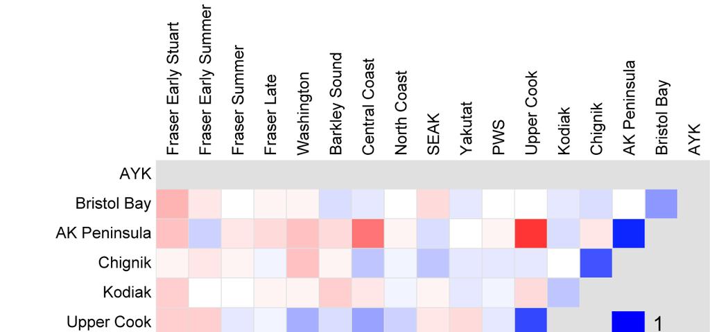
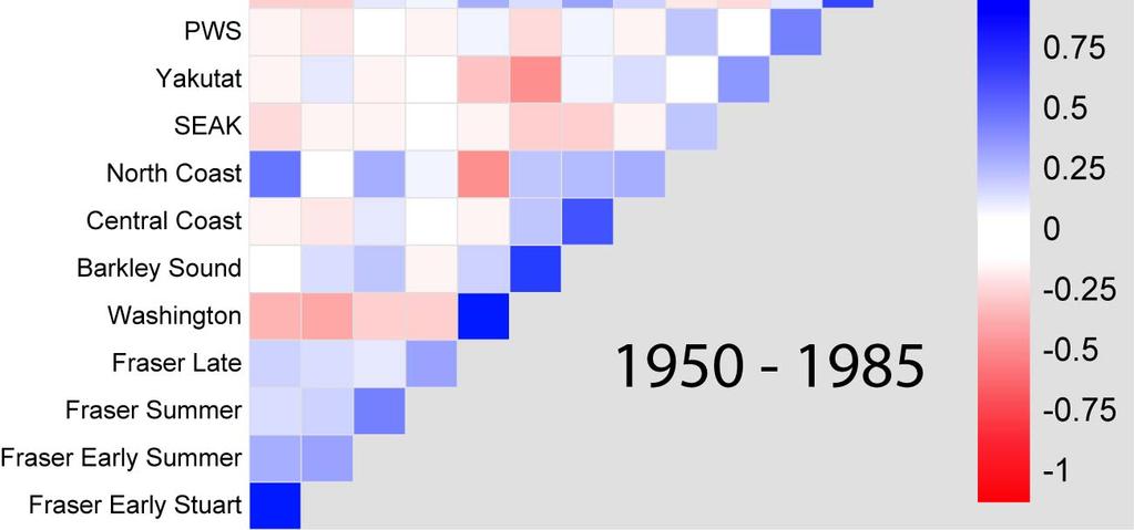
129 126

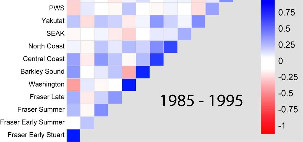
130 127

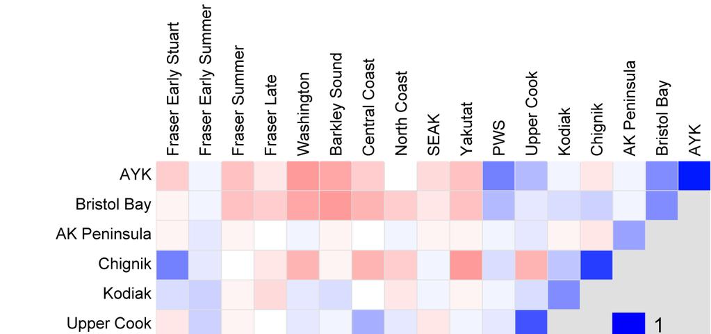
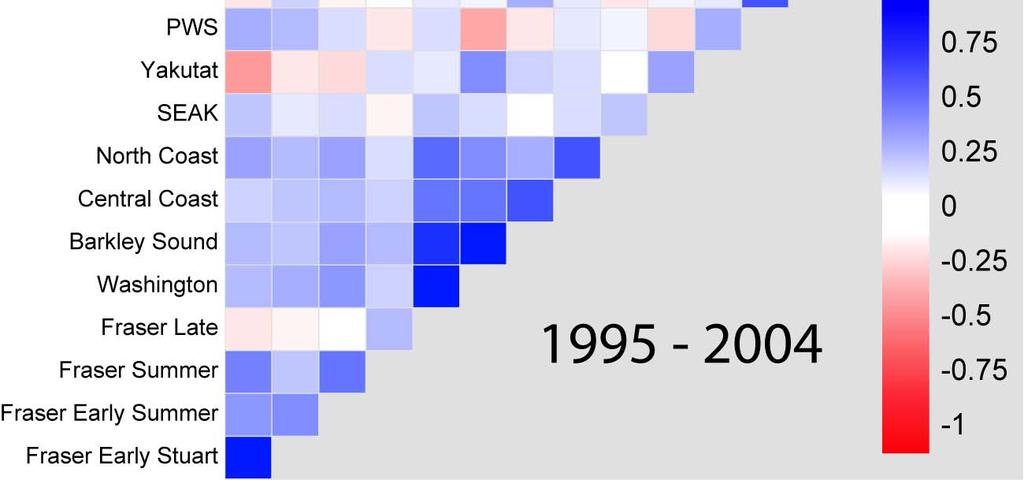
131 128