The Favorite-Longshot Midas

Transcription

1 The Favorite-Longshot Midas Etan A. Green 1, Haksoo Lee 2, and David Rothschild 3 1 University of Pennsylvania 2 Stanford University 3 Microsoft Research February 15, 2019 Abstract Deception underlies a classic case of market inefficiency: the favorite-longshot bias in horserace parimutuel markets. Racetracks provide bettors with predictions. At some tracks, these predictions are well calibrated, and markets are efficient. Other tracks overestimate the chances of longshots; at these tracks, longshots are overbet. The deception is strategic. Deception facilitates arbitrage, and arbitrage generates additional income for the track. Keywords: brokers, deception, arbitrage, parallax and tax, favorite-longshot bias JEL Classification: D22, D82, D83, L83 Please direct correspondence to: etangr@wharton.upenn.edu. We thank Bosko Blagojević and Will Cai for help with scraping and parsing the data; Joe Appelbaum, Hamsa Bastani, Gerard Cachon, Botond Köszegi, Dorothy Kronick, David Laibson, Simone Marinesi, Cade Massey, Ken Moon, Dave Pennock, Alex Rees-Jones, Joe Simmons, and Ran Spiegler for helpful conversations and comments on previous drafts; and Wharton and Microsoft Research for generous financial support.

2 Profit is sweet, even if it comes from deception. Sophocles 1 Introduction Inefficiencies characterize important financial markets. In the stock market, for instance, excess returns are persistent, rather than fleeting (Mehra and Prescott, 1985, 2003); prices swing wildly, often in the absence of news (LeRoy and Porter, 1981; Shiller, 1981, 1992; Shleifer, 1986); and price movements are predictable over short and long horizons (Fama and French, 1988; Jegadeesh and Titman, 1993, 2011). 1 The consensus explanation is that many traders are irrational (Shiller, 1984; Black, 1986; Shleifer and Summers, 1990; De Long, Shleifer, Summers and Waldmann, 1991). These noise traders rely on faulty heuristics and take advice credulously, and they misprice securities by trading on their systematically biased beliefs. Although arbitrage by more sophisticated investors attenuates the mispricing, various limits, such as transaction costs, illiquidity, and risk, preserve some degree of inefficiency (for a review, see Gromb and Vayanos, 2010). A defining trait of noise traders is their gullibility (Akerlof and Shiller, 2015). In pumpand-dump schemes, for example, conspirators deceive gullible traders into overvaluing an asset (i.e., pump) so as to sell their own holdings at higher prices (i.e., dump). This paper characterizes a parallax-and-tax scheme in which a third-party broker, rather than an investor, deceives noise traders and then profits by taxing trade, rather than trading assets. In a visual parallax, the same object appears in different locations when viewed from different positions. Here, a broker induces different valuations of the same asset from different investors. Common valuations present an obstacle to trade (Tirole, 1982) and, hence, an existential threat to brokers. Deception drives a wedge between valuations, increasing trade and brokerage fees. Pump-and-dump schemes require the perpetrator to take a position in the market, entailing financial risk. They are also illegal. Parallax-and-tax schemes, by contrast, shield the broker from financial risk. If they are illegal, they appear to go unprosecuted. In the leadup to the financial crisis, investment banks and credit-rating agencies misled unsuspecting investors about the risk in mortgage-backed securities. Deceived investors overpriced these securities, generating demand from savvy investors for ways to short them, which the same 1 For reviews, see Barberis and Thaler (2003) and Shiller (2003). 1

3 banks engineered and sold for large fees (Lewis, 2015). Investment banks created arbitrage opportunities by deceiving noise traders, and they profited by taxing the arbitrageurs. We begin with an illustrative model of a brokered market with informed arbitrageurs and credulous noise traders. The broker offers two securities: one that pays out if a given event occurs, and one that pays out if the event does not occur. The true probability of the event, p, is known to the broker and the arbitrageurs but not to the noise traders. The broker announces a prediction, q, which noise traders adopt as their beliefs. Noise traders trade in the first period. If q p, they trade on mistaken beliefs and misprice the securities. In the second period, arbitrageurs partially correct the mispricing. Some bias remains, however, because arbitrageurs pay brokerage fees. In choosing q, the broker balances brokerage fees against the long-term costs of deception, both of which increase in the divergence between p and q. More deception increases arbitrage but also becomes more apparent ex post, decreasing future investment by noise traders. We show that if deception has sufficiently convex costs, the broker will deceive by overestimating unlikely outcomes, generating a favorite-longshot bias. 2 In light of this result, we revisit a classic case of market inefficiency: the favoritelongshot bias in horserace parimutuel markets (Griffith, 1949; Thaler and Ziemba, 1988). In parimutuel markets, bettors place wagers on outcomes (e.g., a given horse winning the race), the broker takes a tax, and the remainder is divided among winning wagers. If bettors are risk neutral and have correct beliefs, then expected returns should be the same for favorites and longshots. Consistent with previous literature, we find that wagers on longshots return far less in expectation than wagers on favorites. Whereas a favorite with 1/1 odds (i.e., that pays a $1 dividend on a winning $1 wager) returns 85 cents on the dollar on average, a longshot with 30/1 odds (i.e., that pays a $30 dividend on a winning $1 wager) returns just 63 cents on the dollar. We show that the favorite-longshot bias arises from a parallax-and-tax scheme. track deceives naive bettors by suggesting inflated probabilities for longshots and depressed probabilities for favorites. This deception induces naive bettors to underbet favorites, which creates arbitrage opportunities for sophisticated bettors and, from that arbitrage, incremental tax revenue for the track. 2 This model is most closely related to a series of papers showing that heterogeneous beliefs can generate a favorite-longshot bias in parimutuel markets (Borel, 1938; Hurley and McDonough, 1995; Ottaviani and Sørensen, 2009, 2010; Gandhi and Serrano-Padial, 2014; Chiappori, Salanié, Salanié and Gandhi, 2019) and in markets for Arrow-Debreu securities (Ottaviani and Sørensen, 2015). Our model incorporates the broker, who induces heterogeneous beliefs through deception. The 2

4 Popular accounts of horserace bettors support a simple typology of sophisticates and naifs. Some bettors receive a volume-based rebate. Others pay the full tax. Some bettors place their wagers electronically. Others line up at the track. Some bettors wait until the minutes or seconds before the race begins to place their wagers i.e., when the live odds best predict the final odds (Ottaviani and Sørensen, 2006; Gramm and McKinney, 2009). Others place their wagers twenty minutes before the race begins. Some bettors train algorithms on expensive databases of race histories. Others do not have well-formed beliefs. Anecdotally, those who receive the rebate, who wager electronically, who time their bets strategically, and who analyze data tend to be the same bettors. 3 Tracks provide bettors with a prediction for each horse, in the form of odds. These morning-line odds have no formal bearing on the parimutuel odds. Instead, their ostensible purpose, according to oddsmakers, is to predict, as accurately as possible, how the betting public will wager on each race i.e., to predict the final parimutuel odds. 4 We show that the morning-line odds are miscalibrated: they are insufficiently short for favorites and insufficiently long for longshots. Horses with 1/1 morning-line odds begin the race with parimutuel odds of 1/2, on average; horses with 30/1 morning-line odds end up with parimutuel odds longer than 50/1. If the track is to be believed, and if bettors are risk neutral, then a 1/1 favorite should win about half the time. In practice, horses with morning-line odds of 1/1 win nearly two in three races, yet morning lines are rarely shorter than 1/1. Similarly, a 30/1 longshot should win about 3% of the time. In practice, horses with 30/1 morning-line odds win about 1% of the time, yet morning lines are rarely longer than 30/1. The morning-line odds underestimate the chances of favorites and overestimate the chances of longshots. In other words, they embed a favorite-longshot bias. Across tracks, the extent of the miscalibration in the morning-line odds predicts the extent of the favorite-longshot bias in the parimutuel odds. Some tracks provide well-calibrated 3 From twinspires.com, the online betting platform owned by Churchill Downs, Late odds changes continue to confuse and confound horseplayers...there are big players in the pools and they are called whales. Some whales, not all, use computer software to handicap and make their bets. Because of the volume of the whales play, they are given rebates by advance deposit wagering companies to stimulate more betting. A Bloomberg profile on Bill Benter, whose algorithm made nearly $1 billion betting in horserace parimutuel markets, writes, The odds change in the seconds before a race as all the computer players place their bets at the same time. the-gambler-who-cracked-the-horse-racing-code. 4 Quoted in Getting a Line on the Early Odds, by Joe Kristufek. node/ Similarly, the horse racing columnist Bob Ehalt writes, The intent [of the morning lines] is to frame how the betting on the race will unfold morning-line-odds-betting-tool. Also see: Snyder (1978, p. 1117). 3

5 morning-line odds, and parimutuel odds at those tracks do not exhibit a favorite-longshot bias. Other tracks embed a severe favorite-longshot bias in the morning-line odds, and parimutuel odds at those tracks reflect a severe favorite-longshot bias. These contextual details and stylized facts motivate an application of our two-period brokerage model. In the first period, noise traders infer beliefs, q, under the assumption that the morning-line odds reflect wagering by risk-neutral bettors. Noise traders then wager in proportion to these beliefs, generating odds that reproduce any bias inherent in the morning lines. In the second period, arbitrageurs infer beliefs, p(q), from the observed rates at which horses with implied probability q actually win. Given that the morning-line odds embed a favorite-longshot bias, this correction leads arbitrageurs to view favorites as underpriced, and with the rebate, perhaps profitably so. The track sets the income-maximizing rebate, and a large number of arbitrageurs place all wagers with positive expected value until no more exist. Late wagering concentrates on favorites, and the favorite-longshot bias moderates. The bias does not disappear, however, because arbitrageurs pay some tax. Deceptive morning lines generate excess profit for the track. State-regulated tax rates cap the losses that noise traders should sustain. Deceived traders overbet losers and sustain losses in excess of these caps. Because arbitrage is competitive, these excess losses flow in their entirety into the track s coffers, laundered through taxes on arbitrageurs. We use our model to estimate each track s incremental income from deception. For tracks that embed a favorite-longshot bias in the morning-line odds, we find that as much as 12% of their gambling income comes from taxing arbitrage. A large empirical literature on the favorite-longshot bias in horserace betting markets uses parimutuel odds to estimate the preferences or beliefs of bettors. In this literature, a model is proposed which allows for a downward sloping relationship between the final odds and expected returns. At least one parameter is tuned to match the data. Parameter estimates are then interpreted as evidence of risk-loving preferences (Weitzman, 1965; Ali, 1977; Golec and Tamarkin, 1998), a bias towards overweighting small probabilities (Snowberg and Wolfers, 2010), or heterogeneity in beliefs (Gandhi and Serrano-Padial, 2014) or preferences (Chiappori, Salanié, Salanié and Gandhi, 2019). 5 probability weighting is needed to match the data. 6 Chiappori et al. (2019) conclude that 5 For a more detailed review of the explanations offered for the favorite-longshot bias, see Ottaviani and Sørensen (2008). 6 From page 4: Models relying on an expected utility (EU) framework do not perform well; their fit is quite poor, even for heterogeneous versions of the model...our preferred models are relatively parsimonious versions of homogeneous rank-dependent expected utility (RDEU) preferences, and of homogeneous NEU preferences. In both cases, the main role is played by distortions of probabilities. 4

6 By comparison, our model is restricted in three ways. First, it predicts returns from the formally irrelevant morning-line odds, not the final parimutuel odds. Second, the only parameters in our estimation routine are the hyperparameters we use to (non-parametrically) estimate the beliefs of sophisticated bettors. Third, all agents are risk neutral, and none transforms probabilities. Despite these handicaps, our model closely predicts the observed relationship between odds and returns, outperforming representative-agent models with risk-loving preferences or probability weighting. Moreover, our model predicts the observed variation in the favoritelongshot bias across tracks. In other models, this variation can only be rationalized by trackspecific belief or preference parameters. In our model, variation in the favorite-longshot bias arises from variation in the extent to which tracks overestimate the chances of longshots. The favorite-longshot bias in horserace parimutuel markets is commonly cited as realworld evidence of prospect theory of risk-loving preferences in the domain of losses (Thaler, 2015) or a tendency to overweight small probabilities (Barberis, 2013). We show that neither need be true. Our rendering requires only that some bettors be gullible, rather than speculative or innumerate. Our model also explains three stylized facts that have puzzled researchers for decades. First, prediction markets do not reliably exhibit a favorite-longshot bias. 7 We observe that brokers do not mediate trade in prediction markets. Second, horserace parimutuel markets in Hong Kong and Japan do not exhibit a favorite-longshot bias (Busche and Hall, 1988; Busche, 1994). We observe that race cards in Hong Kong and Japan do not display morning lines. 8 Third, the bias at North American racetracks has moderated over time. In the 1980s, expected returns on a 1/1 favorite and a 50/1 longshot differed by 50 cents on the dollar (Thaler and Ziemba, 1988); they now differ by 35 cents. We suspect that this is due to technologies that facilitate arbitrage in particular, rebates to online bettors. Rebates increase arbitrage volume, which moderates the bias. They also reduce the optimal amount of deception. Absent rebates, arbitrageurs participate only when the track skews the odds such that some wagers promise excess returns, as was true of extreme favorites in the 1980s (Thaler and Ziemba, 1988). When arbitrageurs receive rebates, arbitrage volume can be 7 In prediction markets, the favorite-longshot bias is sometimes present (Wolfers and Zitzewitz, 2004), sometimes absent (Servan-Schreiber, Wolfers, Pennock and Galebach, 2004; Cowgill and Zitzewitz, 2015), and sometimes reversed (Cowgill, Wolfers and Zitzewitz, 2009). Illiquidity and transaction costs are thought to explain inefficiencies in prediction markets (Wolfers and Zitzewitz, 2006). 8 Hong Kong race cards can be accessed at: RaceCard/english/Local/. Japan race cards can be accessed at result/. 5

7 high even when all wagers lose money in expectation. Past studies of the favorite-longshot bias in horserace parimutuel markets ignore the morning-line odds. 9 One reason is that historical morning lines are difficult to obtain. Whereas data on race outcomes, such as the final parimutuel odds, are freely available on the web, historical morning-line odds are only available in an expensive database that is marketed to sophisticated bettors. We collect the morning-line odds by scraping them each morning for over a year. A second reason is that the formal irrelevance of the morning lines appears to have persuaded some scholars of their economic irrelevance. For instance, Ottaviani and Sørensen (2009, p. 2129) justify studying racetrack parimutuel markets because of the absence of bookmakers (who could induce biases). We show that the morning-line odds, devised by the track oddsmaker, induce a favorite-longshot bias. Our model of deception by brokers is distinct from models of deception by firms (Gabaix and Laibson, 2006; Carlin and Manso, 2010; Spiegler, 2011; Heidhues, Kőszegi and Murooka, 2016; Heidhues and Kőszegi, 2017; Kondor and Köszegi, 2017). In these models, profits on naive customers typically offset losses on sophisticated customers. 10 In our model, the broker profits from both naive and sophisticated investors. A similar distinction applies to fixed-odds betting markets, in which a bookmaker, rather than the market, sets the odds. 11 Bookmakers generate excess returns by taking risky positions against bettors with inaccurate beliefs, while using the tax to limit betting by sharps (Levitt, 2004). In our model, the track encourages the sharps to participate and generates a riskless profit by taxing them. The remainder of the paper is organized as follows. Section 2 presents our model of a brokered market with two parimutuel securities. Section 3 describes the empirical context and the data. Section 4 illustrates the favorite-longshot bias and other stylized facts. Section 5 generalizes our model for an arbitrary number of securities, Section 6 compares theoretical predictions with the data, and Section 7 estimates income from deception at each track. Section 8 concludes. 9 To our knowledge, the lone exception is Snyder (1978), who collects the morning-line odds by hand and puzzles over the fact that they reflect a favorite-longshot bias. 10 For instance, Gabaix and Laibson (2006) model a firm that shrouds add-on costs, such as high-priced printer toner. It loses money from sophisticated customers, who only purchase the subsidized printers, and makes money from naive customers, who purchase the toner as well. 11 In fixed-odds betting markets, returns for favorites outpace returns for longshots in horserace betting (Jullien and Salanié, 2000; Snowberg and Wolfers, 2010), but the reverse is generally true for professional American sports (e.g., Gandar et al., 1988; Woodland and Woodland, 1994; Levitt, 2004; Simmons et al., 2010). For models of pricing in fixed-odds markets, see: Shin (1991, 1992); Ottaviani and Sørensen (2005). 6

8 2 Theoretical framework A broker offers two parimutuel securities whose returns are pegged to a binary event. One security pays off if the event occurs; the other pays off if the event does not occur. Let the probability of the event be p 1. Since the event is (weakly) more likely to occur than not, 2 the security tied to the event is the favorite, and the other security is the longshot. The broker announces a prediction for the favorite, q, which a gullible subset of investors take at face value. We are interested in the broker s choice of q Set-up In a parimutuel market, investors purchase shares of a security for a set price (e.g., $1), the broker takes a fee, σ, and the remaining investment is split among shareholders of the security that pays out. Let s be the share of investment in the favorite. If the event occurs, each dollar invested in the favorite returns (1 σ)/s, and investments in the longshot return 0. If the event does not occur, each dollar invested in the longshot returns (1 σ)/(1 s), and investments in the favorite return 0. The more invested in a security, the lower its returns. We consider a two-period model with two types of investors: noise traders and arbitrageurs. Noise traders invest in the first period; arbitrageurs invest in the second. Noise traders are gullible. Absent beliefs about p, they take the broker s prediction, q, at face value i.e., they believe that the event will occur with probability q. Noise traders are also myopic: they fail to anticipate how the parimutuel returns will change in the second period. 13 In the first period, noise traders invest in the security with the higher expected value according to their adopted beliefs. Given the brokerage fee, σ, both securities may portend losses. We rationalize the decision to invest with an additive utility shock, u, consistent with a direct utility from gambling (Conlisk, 1993), and we allow the shock to vary across noise traders. Thus, noise trader j values a $1 investment in the favorite at q(1 σ)/s + u j and a 12 The broker s prediction is cheap talk. We do not write down a cheap talk signaling game (e.g., Crawford and Sobel, 1982) because cheap talk games cannot rationalize biased signals, which we observe in our data. In a cheap talk signaling game, the receiver knows the bias and subtracts it out. Instead, we assume that some investors are gullible. This is similar in spirit to a cursed equilibrium (Eyster and Rabin, 2005), in which agents ignore the signal, though diamatrically opposed in practice here, agents ignore their prior. 13 It is straightforward to write down an alternative model in which noise traders correctly forecast secondperiod investment. In such a model, noise traders invest entirely in the longshot if q < p and entirely in the favorite if q > p; arbitrageurs invest in the other security; arbitrage volume is higher; and broker income is higher as a result. We view this model as implausible because it requires noise traders to know how q compares to the truth and to invest according to q anyway. In other words, one cannot be gullible without also being myopic. 7

9 $1 investment in the longshot at (1 q)(1 σ)/(1 s) + u j. A large number of noise traders each decide whether to invest a $1 endowment, and if so, which security to purchase. We are interested in s, the Walrasian equilibrium share of first-period investment in the favorite. In the second period, arbitrageurs invest in the security with excess returns. Let x be the amount invested by arbitrageurs in the favorite, and let y be the amount invested by arbitrageurs in the longshot. Normalizing the total investment by noise traders to 1, total investment after arbitrage is 1 + x + y, and final parimutuel returns on a $1 investment are (1 σ)(1+x+y)/(s +x) for the favorite and (1 σ)(1+x+y)/(1 s +y) for the longshot. Unlike noise traders, arbitrageurs know p, and they do not receive direct utility from investing. The expected return on a $1 investment in the favorite is: E [ V ($1 in favorite) ] = p(1 σ) 1 + x + y s + x And the expected return on a $1 investment in the longshot is: E [ V ($1 in longshot) ] = (1 p)(1 σ) 1 + x + y 1 s + y The broker price discriminates by offering arbitrageurs a rebate, r, on each dollar invested regardless of the outcome. Hence, the broker s income is: π(r) = σ 1 + (σ r)(x + y) For each dollar invested by noise traders, the broker takes a share σ and arbitrageurs invest x + y dollars, of which the broker takes a share, σ r. We assume that σ is fixed, as when brokers perfectly compete for noise traders or when its fees are regulated. However, the broker holds a monopoly over its own securities, and as such, chooses r to maximize π. We assume that arbitrage is competitive. Hence, the second-period equilibrium is defined by arbitrage volumes {x, y } 0 and a rebate r such that: 1. Arbitrageurs make zero profits in expectation. E [ V ($1 in favorite) ] = $1 r when x > 0 E [ V ($1 in longshot) ] = $1 r when y > 0 2. Arbitrageurs leave no money on the table. E [ V ($1 in favorite) ] $1 r when x = 0 8

10 E [ V ($1 in longshot) ] $1 r when y = 0 3. The broker chooses the income-maximizing rebate: r = arg max r π(r) 2.2 Equilibria In the first-period Walrasian equilibrium, s = q, and only those for whom u j > σ invest. Consider an example with σ = 0.2 and p = 0.6. If the broker predicts q = 0.5, noise traders split their investment evenly among the securities. For a $1 investment on either the favorite or the longshot, the parimutuel advertises a return of (1 σ)/q = (1 σ)/(1 q) = $1.60 were the security to pay out, and noise traders expect a return of 1 σ = 80 cents. Noise traders are gullible, and deception by the broker induces them to misprice the securities. In the example above, the true expected returns are p(1 σ)/q = 96 cents for the favorite and (1 p)(1 σ)/(1 q) = 64 cents for the longshot. Let γ 1 be the ratio of first-period expected returns for the favorite and longshot under correct beliefs: γ 1 = p(1 q) q(1 p) If q < p, the expected return on the favorite exceeds the expected return on the longshot i.e., a favorite-longshot bias. And if q > p, the expected return on the longshot exceeds the expected return on the favorite i.e., a reverse favorite-longshot bias. We now characterize equilibrium rebates, arbitrage volumes, parimutuel returns, and broker revenues. Let r be the income-maximizing rebate. When q < p, the brokerage fee on arbitrage is: σ r = (1 σ)(1 p) ( γ1 1 ) When q > p, ( ) 1 σ r = (1 σ)p 1 γ1 In both cases, fees on arbitrage are positive (i.e., r < σ) and proportional to the square root of the first-period bias, γ 1. When the broker tells the truth, arbitrage is free. Arbitrageurs invest in the security that promises excess returns. When the broker un- 9

11 derestimates the favorite, arbitrageurs invest in the favorite: {x, y } = { q ( γ1 1 ), 0 } When the broker overestimates the favorite, arbitrageurs invest in the longshot: {x, y } = { ( ) 1 } 0, (1 q) 1 γ1 In both cases, the volume of arbitrage increases in the first-period bias. When the broker tells the truth, arbitrage volume is zero. Arbitrage attenuates the bias. Arbitrageurs drive down expected returns on the overvalued security to 1 r for every dollar invested, which increases returns on the undervalued security. Let γ 2 be the ratio of second-period expected returns for the favorite and longshot under correct beliefs. Regardless of q, γ 2 = γ 1 Arbitrage narrows, but does not eliminate, the gap in expected returns. When q < p, 1 < γ 1 < γ 1 ; when q > p, γ 1 < γ 1 < 1. In other words, arbitrage brings the ratio of expected returns closer to one. Arbitrage does not equalize expected returns, however, because arbitrageurs pay some fees. Consider the previous example in which σ = 0.2, p = 0.6, and q = 0.5. The broker sets a rebate of 13 cents, and arbitrageurs invest 11 cents in the favorite for every $1 invested by noise traders. Parimutuel returns for the favorite decrease $1.60 to (1 σ)(1+x )/(q +x ) = $1.46, and parimutuel returns for the longshot increase from $1.60 to (1 σ)(1+x )/(q+x ) = $1.78. Expected returns on a $1 investment decrease from 96 cents to 1 r = 87 cents for the favorite and increase from 64 cents to (1 p)(1 σ)(1 + x )/(1 q) = 71 cents for the longshot. The gap in expected returns shrinks by half. Given the optimal rebate, the broker s equilibrium income is: π (q p) = σ + (1 σ) [ 1 ( ) 2 ] pq + (1 p)(1 q) The first term is the broker s income from noise traders, and the second term is income from arbitrageurs. The broker s income from arbitrage is proportional to one minus the squared Bhattacharyya coefficient, which measures the similarity between two distributions. Hence, 10

12 income from arbitrage, and thus total income, is increasing in the divergence between p and q. When the broker tells the truth, the Bhattacharyya coefficient is 1, and π = σ. When the broker lies, the coefficient is less than 1, and π > σ. By assumption, arbitrageurs make exactly zero profits. Hence, the broker s income equals the total losses sustained by noise traders, which exceed the tax, σ. Because arbitrage is competitive, excess losses incurred by noise traders flow in their entirety to the broker. 2.3 Deception How does the broker choose q? Maximal deception, with q = 0, maximizes the broker s income but may not be advisable in the long run. If the event occurs, noise traders will know they were deceived. Even if it does not, large swings in second-period parimutuel returns will arise suspicion. In response, noise traders may seek out predictions from other sources, decide to invest with other brokers, quit investing altogether, or choose to become sophisticated all of which decrease brokerage fees in the future. Less aggressive deception makes statistical inference more difficult and dampens swings in parimutuel returns, and is presumably less costly for the broker. Rather than model these processes from first principles, we instead add a cost function to the broker s income that is increasing in the divergence between p and q i.e., in the degree of deception. In particular, we assume that the cost of deception, C α (q p), is proportional to the Rényi (or α) divergence between p and q: C α (q p) 1 ( ) p α α 1 log q + (1 p)α, α 1 (1 q) α 1 We use the Rényi divergence because it has a single parameter, α 0, which modulates the function s convexity. 14 Its limiting case as α 1 is the Kullback-Leibler divergence: p log[p/q]+(1 p) log[(1 p)/(1 q)]. Figure 1a shows Rényi divergences for different values of α. Regardless of α, the divergence is zero when q = p, positive when q p (strictly so when α > 0), and increasing as q separates from p. For any α, the function is globally convex in q (Van Erven and Harremos, 2014). At q = p, the convexity in q is proportional to α. Figure 1b shows the broker s income, cost, and profit when the cost of deception is proportional to the Kullback-Leibler divergence. Both income and cost increase with distance between p and q. When q is close to p, income increases faster than cost, implying that 14 Incidentally, the Rényi divergence is also commonly described as the most important divergence in information theory (e.g., Van Erven and Harremos, 2014). 11

13 Figure 1: Rényi divergence between q and p = 0.6 for different values of α (a), and broker financials when the cost of deception is proportional to the Kullback-Leibler divergence (i.e., when α 1). (a) Rényi divergence (b) Broker income, cost & profit Note: In (b), σ = 0.2 and C 1 (q p) includes a multiplicative constant of (1 σ)/3. deception is profitable. In general, deception is profitable when the income function is more convex at q = p than the cost function. 15 When deception is profitable, the profit function has two local maxima one when the broker underestimates the favorite and one when the broker overestimates the favorite. Which is preferable? If α = 1, the broker is indifferent between underestimation and over- 2 estimation. Lemma 1. If α = 1 2, then max q p π(q p) C α (q p) = max q p π(q p) C α (q p). Proof. In Appendix A.1. Using this lemma, we show that the broker overestimates the favorite when α < 1 2 underestimates the favorite when α > 1. 2 and Proposition 1. Let q = arg max q π(q p) C α (q p). If α < 1 2, then q p. If α > 1 2, then q p. 15 This implies an upper bound on the coefficient of proportionality of (1 σ)/2α. 12

14 Proof. In Appendix A.2. The broker induces a favorite-longshot bias when α is sufficiently high i.e., when deception has sufficiently convex costs. When the costs of deception increase rapidly, the broker underestimates the chances of the favorite. 3 Context and data We examine betting markets for North American horseraces, which are run as parimutuels. As in our model, bettors place wagers on outcomes (e.g., a certain horse winning the race), the track takes a state-regulated share σ known as the takeout, and the remainder is split among wagers on the winning outcome. Let s i denote the share of wagers placed on outcome i. A $1 wager on i returns (1 σ)/s i if i occurs, and it returns 0 if i does not occur. Prospective returns are represented as odds, or as the dividend paid on a winning $1 wager: (1 σ)/s i For example, a winning bet at 2/1 odds pays a $2 dividend for every $1 wagered, along with the principal. Tracks update the parimutuel odds in real time on a central board called the tote board, as well as online, but only the final odds, or those the start of the race, are used to calculate payoffs. Wagers on different types of outcomes are collected in separate pools, and odds are calculated within each pool. Almost all tracks offer win, place, and show pools, in which bets are placed on individual horses, and wagers pay out if the horse finishes first (win), first or second (place), or in the top 3 (show). Tracks also offer a selection of exotic pools, in which payoffs are contingent on multiple outcomes. Exacta, trifecta, superfecta, and hi-5 pools pay out if the bettor correctly predicts the first two, three, four, or five horses, respectively, in order; quinella pools pay out if the bettor correctly predicts the first two horses in any order; and daily-double, pick-3, pick-4, pick-5, and pick-6 pools pay out if the bettor correctly predicts the the winners of two, three, four, five, or six races in a row, respectively In practice, tracks round odds down (to multiples of 5 cents for small odds and to larger multiples for higher odds), a practice known as breakage that slightly increases the track s effective takeout. 17 Many exotic wagers can also be constructed as a parlay, or contingent series, of wagers in other pools. For instance, a daily-double wager is logically equivalent to placing the full wager on a win bet in the first race and then placing any winnings on a win bet in the second race. Previous work finds that daily-double returns are less than those of the equivalent parlay, though not by a statistically significant margin and claims that this constitutes evidence of efficient markets (Ali, 1979). We note that parlays are inefficient and hence, impose limits on arbitrage. Though the takeout is generally higher in exotic pools than in win, place, and show pools, the takeout in any exotic pool is always less than the takeout for the equivalent parlay. For example, paying the daily-double takeout once is less expensive than paying the win takeout twice. 13

15 Most empirical studies of the favorite-longshot bias in horse-racing markets analyze data from the race chart, which summarizes the outcome of a race. We compile a similar dataset by collecting: 1) the final odds for each horse in the win pool, 2) the winning outcomes in each pool, 3) the returns to wagers on those outcomes, and 4) the total amount wagered in each pool. 18 Separately, we collect track- and pool-specific takeout rates from the Horseplayers Association of North America. 19 Figure 2: An example race card entry, prominently displaying the morning-line odds (15-1). Source: Equibase.com We supplement this standard dataset with the morning-line odds, or the formally irrelevant win odds chosen by the oddsmaker at the track. Tracks publish morning lines in three places: 1) online; 2) on the tote board at the beginning of the betting window, when betting volume is low and parimutuel odds are unstable; and 3) in the race card, a printed pamphlet handed out at the track that provides information on each horse in each of the day s races. Figure 2 shows an example race card entry. Whereas historical race charts are freely available, historical race cards are not. Instead, we scraped the morning-line odds each morning for 17 months from 2016 to In order to analyze the data within track, we restrict our sample to the 30 tracks for which we observe at least 5,000 horse starts. Our final dataset comprises 238,297 starts in 30,631 races. 21 Table 1 presents summary statistics by track. Takeouts range from 12% to 31%. For comparison, bookmakers typically take 9% of winnings on common wagers in professional team sports. The takeout is typically smaller in the win, place, and show (WPS) pools than 18 One limitation of these data is that only in the win pool are final odds listed for all outcomes (i.e., horses); in other pools, only the odds for the winning outcome are listed The scraper went offline from December 2, 2016 to July 23, This reflects the discarding of 91,727 starts in 12,164 races at 68 excluded tracks. Scraping or parsing issues led to the exclusion of an additional 4,147 races at both included and excluded tracks. 14

16 Table 1: Summary statistics by track. Track Counts Takeout rates Wager % Code Name State Days Races Starts WPS Quinella Exacta Trifecta Superfecta Hi-5 Daily Double Pick 3 Pick 4 Pick 5 Pick 6 WPS Exotic ALB Albuquerque NM AP Arlington IL AQU Aqueduct NY BEL Belmont NY BTP Belterra Park OH CBY Canterbury MN CD Churchill Downs KY CT Charles Town WV DED Delta Downs LA DEL Delaware DE DMR Del Mar CA EVD Evangeline LA FG Fair Grounds LA FL Finger Lakes NY GG Golden Gate CA GP Gulfstream FL IND Indiana IN LA Los Alamitos CA LAD Louisiana Downs LA LRL Laurel MD MNR Mountaineer WV MVR Mahoning Valley OH PEN Penn National PA PID Presque Isle PA PRX Parx PA RP Remington OK SA Santa Anita CA SUN Sunland NM TAM Tampa Bay Downs FL TUP Turf Paradise AZ

17 in the exotic pools, yet as the final two columns show, more money is wagered in exotic pools at every track. All standard errors reported in the paper either directly in the text or in tables, or as 95% confidence intervals in figures are estimated from 10,000 bootstrap samples blocked by track Stylized facts Figure 3: Expected returns for win bets, with 95% confidence intervals. The horizontal line marks the average takeout. Note: Estimated using a local linear regression with a Gaussian kernel. The bandwidth, of log(1.65), minimizes the leave-one-out mean-squared error. Returns are systematically miscalibrated. Figure 3 shows observed returns in the win pool as a smooth function of log final odds. Wagers at all odds lose money on average, given the large takeouts. However, wagers on horses with longer odds lose more money. A $1 bet on a 1/1 favorite loses 15 cents in expectation, a smaller loss than the average takeout of 22 The standard bootstrapping approach is to resample observations, or in our case, an outcome in a given pool. However, doing so would create bootstrap samples for which the number of winning outcomes in each pool need not be one. As a result, we resample entire pools, rather than individual outcomes. The lone exception is Figure 5, for which the confidence intervals are calculated from homoskedastic standard errors. 16

18 17 cents. By contrast, a 20/1 longshot loses 29 cents, and a 50/1 longshot loses 47 cents. 23 Bettors could reduce their losses by betting on favorites instead of longshots. Figure 4: Returns for win bets, by track. In (b), tracks are sorted by the estimated expected returns at 30/1 odds in (a). (a) Expected returns (b) Normalized mean returns Note: Track-specific expected returns in (a) estimated as in Figure 3. For comparability, we use the same bandwidth as in the full sample, of log(1.65). The extent of the favorite-longshot bias varies across tracks. Figure 4a shows expected returns in the win pool as a smooth function of log final odds, separately by track. (Individual plots are shown in Figure 4a in Section 6.) Some tracks exhibit little or no bias, whereas others exhibit severe bias. We summarize the extent of the favorite-longshot bias at track t by its mean returns, µ t, or the expected return on a $1 wager for a bettor who picks horses at random. A random betting strategy overbets longshots relative to the market. Were horses priced efficiently, overbetting longshots would not incur a penalty. Instead, a random betting strategy would surrender the takeout on average, and µ t would equal 1 σ t. When 23 These estimates are consistent with those from other analyses of parimutuel odds. For instance, Snowberg and Wolfers (2010) estimate expected returns of about 85% for a 1/1 favorite, 75% for a 20/1 longshot, and 55% for a 50/1 longshot. The favorite-longshot bias tends to be more severe in markets where bookmakers set the odds. For instance, Jullien and Salanié (2000) estimate expected returns of close to 100% for 1/1 favorites and 50% for 20/1 longshots using data from the United Kingdom, where all odds are set by bookmakers. 17

19 longshots yield lower returns than favorites, however, overbetting longshots generates excess losses. Hence, a steeper favorite-longshot bias implies lower mean returns, µ t. Figure 4b shows normalized mean returns, µ t /(1 σ t ), by track. 24 The tracks are ordered by their estimated returns at win odds of 30/1, as shown in Figure 4a. For some tracks, expected returns are approximately flat and normalized mean returns are close to 1, implying that wagering randomly does not generate excess losses. For the remaining tracks, estimated returns are greater for favorites than for longshots, and random wagering generates excess losses. These differences across tracks cannot be explained by sampling variation alone. A Wald test rejects the null hypothesis that normalized mean returns, µ t /(1 σ t ), are equivalent at all tracks (p <.001). Figure 5: Average log final odds at each morning-line odds. For all but the shortest odds, the 95% confidence intervals are obscured by the point estimates. The favorite-longshot bias appears to be related to the morning-line odds. One immediate observation is that the morning-line odds fail at their ostensible goal of predicting the parimutuel odds. Figure 5 shows average final odds at each observed morning-line odds. Morning-line odds are compressed on average, those shorter than 4/1 are insufficiently short, and those longer than 4/1 are insufficiently long. For example, favorites assigned morning-line odds of 1/1 finish with final odds of 1/2 on average, and longshots assigned 24 In practice, the track s takeout rate is slightly higher than σ t because of the breakage, the practice of rounding down parimutuel odds, typically to the nearest 10 cents. Figure 4b normalizes mean returns by the true return rate, 1/ i R 1/(O i + 1). 18

20 morning-line odds of 30/1 finish with final odds in excess of 50/1. If oddsmakers are trying to predict final odds, they could do better by predicting more extreme values. Figure 6: Time series of the log ratio of live parimutuel odds to morning-line odds, separately for the favorite and longshot (as defined by the morning lines). Note: These estimates reflect second-by-second averages over 1,362 races in 2017 and 2018 for which at least 20 time-stamps were observed during the last 60 minutes of the betting window, and for which the morning-line odds uniquely define a favorite and a longshot. We interpolate missing time-stamps by assigning the most recently observed live odds. The parimutuel odds diverge from the morning lines just before the start of the race. Figure 6 plots a time series of live odds from a separate dataset of 1,362 US races. We plot the average log ratio of parimutuel odds to morning-line odds in the hour before the race, separately for the favorite and the longshot (as defined by the morning-line odds). On average, the parimutuel odds for the favorite and longshot hover around their respective morning-line odds until about 15 minutes before the start of the race. Thereafter, the longshot s odds lengthen and the favorite s odds shorten, implying late wagering on favorites (see also: Asch, Malkiel and Quandt, 1982; Camerer, 1998). The morning-line odds not only mispredict the final odds they also imply distorted beliefs about a horse s chances of winning. Imagine that bettors place wagers such that the parimutuel odds converge to the morning lines, as the track oddsmaker predicts. If these bettors are risk neutral, then the expected value of betting on any horse given subjective 19

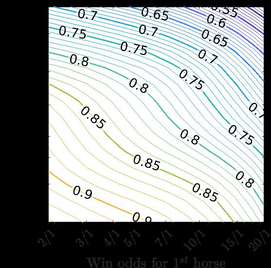
21 beliefs q must be the same for all horses in the race. That is, q i (l i +1) = q j (l j +1) i, j R, where R is the set of horses in a race, and l + 1 is the return on a winning $1 wager. Given that j R q j = 1, the subjective probability of horse i winning is: q i = 1 / 1 l i + 1 l j + 1 j R (1) The beliefs implied by the morning-line odds are simply the inverse of the associated returns on a $1 wager, normalized such that these beliefs sum to Figure 7: Observed win rate, p, as a function of the win probability implied by the morningline odds, q, with a histogram of q. These beliefs are misleading. Figure 7 shows a calibration plot the observed win rate (denoted by p) as a smooth function of q, the win probabilities implied by the morning-line odds. 26 Longshots underperform their implied win probabilities, q. At q = 0.03, for example, 25 Typically, the inverse implied returns sum to about 1/(1 σ t ) i.e., the morning-line odds are odds that could occur in the parimutuel. 26 We are interested in estimating a smooth function, p(q), that measures the rate at which horses with an implied probability of winning, q, actually win the race. To do so, we regress an indicator for whether the observed horse won the race on log q, its log probability of winning, as implied by the morning-line odds and as calculated in (1). In particular, we use the Nadaraya-Watson estimator, otherwise known as local constant regression, which unlike a local linear or local polynomial regression, ensures that the predicted values stay between the bounds of the outcome variable i.e., between 0 and 1. The challenge is that we would like p(q) to be weakly increasing, reflecting an assumption that the morning lines correctly order the horses by 20

22 horses win just 1 in 100 races; at q < 0.03, horses effectively never win. Morning-line odds of 30/1 imply win probabilities of q Of the 7,869 starts assigned 30/1 morning-line odds, just 83, or 1.1%, won the race. Morning-line odds of 50/1 imply win probabilities of q Of the 586 starts assigned morning-line odds longer than 50/1, just 2, or 0.3%, won the race. Symmetrically, favorites outperform their implied win probabilities. At q = 0.5, for example, p = The morning-line odds mislead at some tracks but not at others. Figure 8 replicates the estimate of p separately by track. Some tracks post well-calibrated morning-line odds (e.g., PRX), whereas others post misleading morning-line odds (e.g., LA). Tracks that promulgate distorted predictions deceive bettors in the same manner by assigning insufficiently long morning lines to longshots and insufficiently short morning lines to favorites. In other words, these tracks embed a favorite-longshot bias in the morning-line odds. Across tracks, miscalibration in the morning-line odds predicts the favorite-longshot bias. As before, we measure the extent of the favorite-longshot bias using the normalized mean returns, or µ t /(1 σ t ) in Figure 4b. Miscalibration is measured as follows. Let p t (q j ) be the empirical rate at which a horse with implied probability q j at track t wins, as shown in Figure 8, and let p j be the normalized rate such that j R p j = 1. We measure miscalibration in a given race as the Kullback-Leibler divergence between the vector of implied winning probabilities, q j, and the corresponding vector of normalized winning rates, p j : j R p j log(p j /q j ). If q = p for each horse in the race, the divergence is zero; otherwise it is positive. We then define the miscalibration at track t, denoted δ t, as the average Kullback- Leibler divergence among races at that track. Figure 9 shows a strong correlation between δ t and µ t /(1 σ t ). The more severe the miscalibration in the morning-line odds, the more severe the favorite-longshot bias. It is unclear why miscalibration in the morning-line odds varies across tracks. There are too few tracks in North America let alone in our data to identify correlates of mistheir chances of winning, even if they imply poorly calibrated beliefs. To do so, we follow Hall and Huang (2001) in assigning each observation a weight between 0 and 1, and, via quadratic programming, minimizing the Kullback Leibler divergence of the weight vector, subject to the constraints that 1) the function p(q), estimated at every half-percentage-point value of q, is weakly increasing; and 2) the weights sum to 1. This routine does not guarantee convergence. For instance, if a lone horse with a high implied win probability q did not win its race, the monotonicity constraint will force the weight on this observation to 0, sending the Kullback Leibler divergence to infinity. To avoid this pitfall, we employ a bandwidth hλ(x), where h is a scalar bandwith, and λ is a local bandwidth factor that increases the bandwidth in regions of low density. This multiplicative factor is λ(x) = exp ( 1 N i log f(log q i ) ) / f(x), where f is a kernel density estimate of log q using Silverman s rule-of-thumb bandwidth. The steps are as follows. We find the bandwidth, h, that minimizes the leave-one-out mean-squared error. Fixing the bandwidth, we then find the vector of minimally divergent weights that satisfy the weak monotonicity condition. 21

23 Figure 8: Observed win rate (p) as a function of the win probability implied by the morningline odds (q), by track. The gray outline shows a histogram of q. ALB AP AQU BEL BTP CBY CD CT DED DEL DMR EVD FG FL GG GP IND LA LAD LRL MNR MVR PEN PID PRX RP SA SUN TAM TUP 22

24 Figure 9: Scatter plot, with a regression fit line, of miscalibration in the morning-line odds, δ t, and normalized mean returns for win bets, µ t /(1 σ t ), across tracks. calibration. Nonetheless, an anecdote suggests one predictor: falling income. Wagering at Canterbury Park (CBY) decreased from 2015 to 2016 even though the track cut its takeouts below state-regulated levels. 27 At the same time, Canterbury Park aggressively overestimated the chances of longshots, as shown in Figure Consistent with our model, a track with good reason to discount the future is among the most misleading. 5 Empirical model These stylized facts motivate an application of our model from Section 2 to horserace parimutuel markets. In this section, we generalize the model to an arbitrary number of outcomes (e.g., horses in a race). This allows us to predict an array of quantities arbitrage volume, optimal rebates, track income, parimutuel odds, and expected returns solely from the beliefs of noise traders and arbitrageurs, which we infer from the morning-line odds At Canterbury, horses with 15-1 morning lines (average q of 5.6%) won 2.8% of races, horses with 20-1 morning lines (average q of 4.2%) won 1.1% of races, and horses with 30-1 morning lines (average q of 2.9%) did not win a race in 97 tries. 23

25 5.1 Setup The set-up is identical to Section 2, with the exception that there are now N 2 outcomes, indexed by i. The track announces predictions q i such that N i=1 q i = 1. In the first period, noise traders take the track s predictions at face value and wager on the outcome with the highest subjective expected value. Noise trader j values a $1 investment in outcome i at q i (1 σ)/(1 s i )+u j, where s i is the share of first-period wagering on outcome i and u j is the direct utility that noise trader j receives from wagering $1. A large number of noise traders each decide whether to wager a $1 endowment, and if so, which outcome to bet on. We are interested in s i, the Walrasian equilibrium share of first-period wagering on each outcome. Arbitrageurs wager in the second period. Unlike noise traders, arbitrageurs know p i, and they do not receive direct utility from gambling. Let x i be the amount wagered by arbitrageurs on outcome i. Normalizing total wagering by noise traders to 1, the expected return on a $1 wager on outcome i is: E[V ($1 on i)] = p i (1 σ) 1 + j x j s i + x i The track price discriminates by offering arbitrageurs a rebate, r, on each dollar wagered regardless of the outcome. For every dollar wagered by noise traders, the track receives: π(r) = σ + (σ r) We assume that arbitrage is competitive. Hence, the second-period equilibrium is defined by arbitrage volumes {x i } 0 and a rebate r such that: 1. Arbitrageurs make zero profits: E[V ($1 on i)] = $1 r when x i > 0 2. Arbitrageurs leave no money on the table: E[V ($1 on i)] $1 r when x i = 0 3. The track chooses the income-maximizing rebate: r = arg max r π(r) N i=1 x i 5.2 Results In the first-period Walrasian equilibrium, s i = q i, and only those for whom u j > σ invest. First-period parimutuel odds are O (1) i = (1 σ)/q i 1. For the second-period equilibrium, we first derive the condition under which one exists. 24

26 Lemma 2. Reorder the outcome indices i such that: p 1 q 1 p 2 q 2 p i q i p i+1 q i+1 p N q N An equilibrium exists if and only if there exists an index m such that: p m q m > P m (1 P m ) Q m (1 Q m ) p m+1 q m+1, (2) where P m m i=1 p i and Q m m i=1 q i. In this equilibrium, x i > 0 for i m and x i = 0 for i > m. Proof. In Appendix A.3. The index m separates outcomes that arbitrageurs wager on from those they do not. P m and Q m are the cumulative subjective probabilities held by arbitrageurs and noise traders, respectively among outcomes wagered on by arbitrageurs. Arbitrageurs wager on outcomes for which their own beliefs are high relative to those of noise traders. Corollary 1. P m Q m. Proof. In Appendix A.4. Under a mild condition, an equilibrium exists: Proposition 2. If p 1 > q 1, then there exists an m {1,..., N 1}. Proof. In Appendix A.5. An equilibrium exists so long as subjective beliefs do not coincide for every outcome i.e., if p 1 > q 1 (and hence, p N < q N ). If so, m 1, implying that arbitrageurs always wager on the outcome with the highest ratio of subjective beliefs. In addition, m < N, implying that arbitrageurs never wager on the outcome with the lowest ratio of subjective beliefs. Equilibrium wagers by arbitrageurs are: x i = p i Q m (1 Q m ) P m (1 P m ) q i for i {1,..., m} (3) 25

27 and x i = 0 for i {m + 1,..., N}. The amount wagered by arbitrageurs on outcome i is increasing in its true probability, p i, and decreasing in the beliefs of noise traders, q i, all else equal. Other quantities all have analogous expressions to those in Section 2, with P m replacing p and Q m replacing q. Let: Arbitrageurs collectively wager: γ m P m(1 Q m ) Q m (1 P m ) N x i = Q m ( γ m 1) (4) i=1 Let r be the revenue-maximizing rebate. Then, σ r = (1 σ)(1 P m )( γ m 1) (5) And the track s income is: ( π t (r ) = σ + (1 σ) 1 ( Pm Q m + (1 P m )(1 Q m ) ) ) 2, (6) where σ is the track s income from noise traders, and the second term is track s income from arbitrageurs. The track s income from arbitrage is increasing in the divergence between P m and Q m. If P m = Q m, which occurs only when p i = q i for all i, arbitrageurs place zero wagers, and the track generates zero income from arbitrage. Deviations between p i and q i, and hence between P m and Q m, generate wagers from arbitrageurs and profits for the track. The final parimutuel odds are: [ 1 Pm p i = (1 σ) i + (1 P m ) ] γ m 1, i {1,..., m} [ 1 Qm γm q i + (1 Q m ) ] 1, i {m + 1,..., N} O (2) (7) Without a rebate, the true expected value of a $1 wager on outcome i is: P m + (1 P m ) γ m, i {1,..., m} E[V ($1 on i)] = (1 σ) p i [ Qm γm q i + (1 Q m ) ], i {m + 1,..., N} (8) 26

28 Arbitrage equalizes returns among outcomes on which arbitrageurs wager. A $1 wager on any of the first m outcomes has an expected return of $1 r. For i > m, wagers perform worse in expectation, following from (2), and they perform progressively worse as i increases, given that p i /q i decreases in i. It is straightforward to see how a favorite-longshot bias in the track s predictions manifests in the parimutuel odds. A favorite-longshot bias characterizes the track s predictions if p 1 p 2 p N, as this implies that the track underestimates the favorite (p 1 > q 1 ) and overestimates the longshot (p N < q N ). Further assume that q 1 q 2 q N i.e., the track s predictions correctly order the outcomes by their true probabilities. Given that the parimutuel odds in (7) are inversely proportional to p i, this indexing orders outcomes by their odds, from short to long. For outcomes with shorter odds (i.e., i m), expected returns are flat. For outcomes with longer odds (i.e., i > m), expected returns are decreasing. Hence, the relationship between odds and expected returns is piecewise linear, similar to that observed in Figure 3, with the kink located at the odds of outcome m. 5.3 Estimation We infer the beliefs of noise traders by assuming that they take the morning-line odds at face value i.e, as a well-calibrated, or unbiased, prediction of the parimutuel odds in the win pool. Specifically, noise traders form beliefs q i,win as in (1) i.e., by inverting the morning lines and then normalizing by race such that i R q i,win = In contrast, we imbue arbitrageurs with well-calibrated beliefs, p i,win. Specifically, we non-parametrically estimate the track-specific rates at which horses associated with similar naive beliefs, q i,win, actually win the race, as shown in Figure 8 and described in Footnote 26. We then normalize these estimates by race such that i R p i,win = Whereas noise traders assume that the morning lines imply well-calibrated beliefs, arbitrageurs ensure that their beliefs are well calibrated. We use these beliefs to construct beliefs for exotic outcomes. In doing so, we adopt the Harville assumption: the probability of a horse finishing in n th place is simply its probability of winning the race, divided by the cumulative winning probability among horses that did not finish in the first n 1 positions (Harville, 1973). The race for second place, for instance, 29 In the win pool, noise traders need not form these beliefs explicitly. They behave as if maximizing expected value given q i,win by simply wagering on the horse with the highest ratio of morning-line odds to current parimutuel odds. 30 Because this routine is computationally intensive, we do not repeat it during bootstrapping. Instead, we use the same estimates of p i (and q i ) in every resampled race. 27

29 can be thought of as a race within a race in which the first-place finisher does not participate. We first consider place and show wagers, which pay out if the chosen horse finishes in the top 2 or 3 positions, respectively. The probability of a place wager on horse i paying out is: p i,place = p i,win + j i p j,win p i,win 1 p j,win where the second term is the probability of horse i finishing second. Beliefs for noise traders, q i,place, can be calculated in a corresponding manner. Similarly, the probability of a show wager on horse i paying out is: p i,show = p i,place + j i k (i,j) p j,win p k,win p i,win 1 p j,win 1 p j,win p k,win where the second term is the probability of horse i finishing third. We also consider a range of exotic wagers. Bettors may wager on the order of the first n horses in a single race, as in exacta and trifecta pools, which we denote by order-n. The probability of a sequence, v, is: p v 2,win p order-n ( v) = p v1,win 1 p v1,win p vn,win 1 p v1,win p vn 1,win A variant of the exacta (i.e., order-2) is the quinella, in which the bettor predicts the first two horses regardless of order. Assuming conditional independence, the probability of a quinella bet on (i, j) paying out is: p j,win p i,win p quin (i, j) = p i,win + p j,win 1 p i,win 1 p j,win This is equivalent to the probability that an exacta bet on either (i, j) or (j, i) pays out. Bettors may also wager on the winner of n consecutive races, as in daily-double and pick- 3 pools, which we denote by pick-n. Assuming independence between races, the probability of a sequence, v, is: p pick-n ( v) = n i=1 p (i) v i,win where the superscript indexes the race. Finding the equilibrium in each pool proceeds according to the model. We order outcomes 28

30 by p i /q i, from greatest to smallest. Using a grid search, we find the index m that satisfies the relationship in (2); if more than one such index exists, we choose the one that maximizes track income. 31 For each outcome, we calculate the equilibrium odds in (7) and expected returns in (8). In Section 6, we compare the relationship between equilibrium odds and expected returns predicted by our model to that observed in the data. We then calculate the optimal rebate from (5), which unlike the takeout is unobserved, and track revenues under the optimal rebate (6), which we report in Section Example Table 2 illustrates the estimation routine for an example race at Charles Town. T Rex Express, the favorite with 1/1 morning-line odds, finished with final odds of 3/10 on the tote board and in first place on the track. As a result, win bets on T Rex Express paid out a divided of 30 cents on every dollar wagered. Relative to the morning lines, parimutuel odds lengthened for the other six horses in the race. Table 2: Example race at Charles Town. Odds Beliefs Model predictions in win pool Name M/L Final q i p i p i /q i O (1) i E (1) i x i O (2) i E (2) i T Rex Express 1/ Tribal Heat 2/ Dandy Candy 6/ Click and Roll 8/ Eveatetheapple 20/ Movie Starlet 20/ Boston Banshee 30/ In other words, we consider the equilibrium under the income-maximizing rebate. In the data, 37% of pools have more than one equilibrium. Multiple equilibria are most common for pick-n bets, occurring in 50% of such pools. They are least common for win, place, and show bets, occurring in 32% of those pools. 32 The expressions for equilibrium quantities are slightly different in place and show pools, where more than one outcome obtains. Let k denote the number of outcomes that pay out i.e., k = 2 in place pools and k = 3 in show pools with i q i = i p i = k. Observe that the parimutuel pays out 1/k th of the post-tax pot to winning wagers. Hence, second-period odds can be written as: O (2) i = 1 t k 1 + x 1, q i /k + x i Modified expressions for the equilibrium odds, expected returns, optimal rebate, and track revenues can be derived in the same manner. 29

31 The beliefs ascribed to noise traders, q i, are those that a representative risk-neutral bettor would hold if the final odds coincided with the morning-line odds. Specifically, they are inversely proportional to the returns implied by the morning-line odds, up to a normalizing constant, as in (1). By contrast, the beliefs ascribed to arbitrageurs, p i, are well calibrated i.e., proportional to the track-specific rates at which horses with implied beliefs q i actually win, as shown in Figure 8, up to a normalizing constant. For Charles Town, beliefs of q i > 0.2 are too pessimistic on average, and beliefs of q i < 0.2 are too optimistic on average. As a result, p i > q i for T Rex Express (q = 0.41) and for Tribal Heat (q = 0.27), and p i < q i for the other 5 horses. The first-period odds in the win pool, O (1) i, reflect betting by risk-neutral noise traders, given beliefs q i. They diverge from the morning-line odds only because the morning-line odds do not precisely reflect the takeout, of 17.25%, and the breakage, the practice of rounding down odds to the nearest 10 cents. The first-period odds generate a severe favorite-longshot bias. The first-period expected returns on a $1 wager denoted E (1) i and taken over p i are sharply decreasing in the odds. At first-period odds of 1.0, the p = 0.52 favorite is better than an even money bet. By contrast, at odds of 20.1, the p = 0.01 longshots return just 28 cents on every dollar wagered and the p = 0 longshot returns 0 at any odds. The second-period equilibrium consists of a set of wagers by arbitrageurs, x i, such that they make zero profits and leave zero profits on the table. To find this equilibrium, we sort the outcomes in descending order of p i /q i and find the equilibrium index m. In the example above, this ordering coincides with sorting the horses in ascending order of the morningline odds a product of the favorite-longshot bias embedded in the morning lines. equilibrium m = 4 is unique, implying that x i > 0 for the first 4 horses and x i = 0 for the remaining 3. Second-period wagers concentrate on the favorite, and the predicted odds, O (2) i, shorten for the first two horses and lengthen for all others. A less severe favorite-longshot bias remains. For any of the first three horses, the expected returns on a $1 wager, E (2) i, is 85 cents, with the 15-cent expected loss equaling the optimal rebate. For the longshots, expected losses attenuate in the second period. A $1 wager on either of the horses with 20/1 morning lines, for instance, returns 55 cents in expectation at odds of 40.6, or 21 cents more than at first-period odds of In the win pool, arbitrageurs wager 97 cents for every dollar wagered by the noise traders. However, income from arbitrageurs comprises just 12% of the track s total income in the win pool, as the track offers arbitrageurs a 15-cent rebate. Arbitrage accounts for larger shares of the track s income in exotic pools. In the exacta pool, for instance, that share The 30

32 is 21%; in the superfecta pool, it is 41%. The compound beliefs attached to outcomes in exotic pools amplify differences in beliefs about win probabilities between noise traders and arbitrageurs and hence, taxes from arbitrageurs. This logic implies larger divergences between the cumulative beliefs P m and Q m. In the win pool, for example, P m = 0.97 and Q m = 0.90, whereas in the superfecta pool, P m > 0.99 and Q m = Model predictions We begin by comparing predictions from the first- and second-period equilibria. Figure 10 shows a smoothed estimate of the relationship between log predicted odds and predicted returns for win bets, separately by period. (All predicted returns reflect expected returns absent the rebate and under correct beliefs.) In the first-period equilibrium, predicted odds approximate the morning-line odds, which embed a favorite-longshot bias that is more severe than that observed in the data. Figure 10: Predicted and observed returns for win bets. The horizontal line marks the average takeout. Note: Estimated using a local linear regression with a Gaussian kernel. For comparability, we use the same bandwidth for the predicted estimates as for the observed estimates: the bandwidth used in Figure 3, of log(1.65). The inclusion of arbitrageurs in the second period moderates the favorite-longshot bias, 31

33 and the resulting predictions more closely follow observed returns. For a 1/1 favorite, firstperiod expected returns exceed observed returns by 11 cents; after arbitrage, the difference is 2 cents. For a 30/1 longshot, observed returns exceed first-period expected returns by 19 cents; after arbitrage, the difference is 7 cents. Second-period predictions slightly exaggerate the extent of the bias for reasons that we discuss at the end of this section. We quantify the goodness of our model s predictions by measuring the expected absolute deviation: the average distance between predicted and observed returns, with the expectation taken over the distribution of observed odds. 33 For a bettor who wagers randomly, the absolute difference between her returns and those predicted by the model converges asymptotically to our expected absolute deviation measure. This measure is just 3.1 (se: 0.5) cents for the model s second-period predictions, compared to 9.7 (se: 1.6) cents before arbitrage. Figure 11: Predicted returns for win bets from models with non-standard agents. Note: Estimated using a local linear regression with a Gaussian kernel. For comparability, we use the same bandwidth for the predicted estimates as for the observed estimates: the bandwidth used in Figure 3, of log(1.65). Representative-agent models perform worse. Previous work has rationalized the favoritelongshot bias with risk-loving preferences (e.g., Weitzman, 1965; Ali, 1977) or a tendency to overweight small probabilities (e.g., Snowberg and Wolfers, 2010). Figure 11 shows predicted 33 We estimate this distribution using a kernel density estimator with Silverman s rule-of-thumb bandwidth. 32

34 returns from each model. 34 For both models, predicted returns for favorites exceed observed returns, and the overall fit is poor. Expected absolute deviations, of 9.2 (0.5) cents for the risk-loving model and 7.0 (0.4) cents for the probability-weighting model, exceed the 3.1-cent deviation from our model with arbitrage. The difficulty is that neither model can rationalize highly negative returns for probable events. Risk-loving agents pay a large premium for lottery tickets, but they pay a small premium for gambles with little upside. Prospect-theory agents overweight large probabilities and thus need to receive a premium in order to wager on likely events. The decision to gamble is commonly rationalized by risk-loving preferences (e.g., Thaler and Johnson, 1990) or probability weighting (e.g., Barberis, 2012), but neither explanation can account for a willingness to lose considerable sums, in expectation, when wagering on favorites. 35 Our model with arbitrage also captures differences across tracks in the extent of the bias. Figure 12 shows smoothed estimates of the observed and predicted relationships between log odds and expected returns, separately by track. For most tracks, the predicted relationship closely follows the observed relationship. Figure 13 summarizes the model s fit at each track by comparing observed and predicted normalized mean returns i.e., the expected return on a randomly placed $1 win bet, normalized by the state-sanctioned return, 1 σ t. Observed and predicted values are correlated at ρ = 0.63, and predicted values explain 39% of the variation in the observed values across tracks. We evaluate our second-period predictions in other pools as well. Figure 14 shows ob- 34 We estimate these models following Snowberg and Wolfers (2010). In equilibrium, agents wager until the expected utility of a $1 bet equals $1, or until p i U(O i + 1) = 1 i R in the risk-loving model. For the probability-weighting model, the equilibrium condition is π(p i )(O i + 1) = 1 i R. Each model is governed by one parameter. For the risk-loving model, Snowberg and Wolfers (2010) use the CARA utility function U(x) = ( 1 exp( αx) ) /α, where α modulates the agent s risk tolerance. For the probabilityweighting model, they use the weighting function π(p) = exp [ ( log(p) ) β], where β modulates the degree to which the agent overweights small probabilities and underweights large ones (Prelec, 1998). We estimate each model by minimizing the squared distance between observed returns and expected returns, p i (O i + 1), where O i are the observed parimutuel odds, and p i can be found by solving the appropriate equilibrium condition. In the risk-loving model, we estimate ˆα = (0.001), implying an extreme taste for risk. This representative agent is indifferent between $100 for sure and a gamble that pays $123 with 50% probability and $0 otherwise. In the probability-weighting model, we estimate ˆβ = (0.003), implying overweighting of small probabilities. This representative agent behaves as if an event with 1.0% probability occurs 1.9% of the time. These estimates are more slightly more extreme than those of Snowberg and Wolfers (2010), who estimate ˆα = and ˆβ = Snowberg and Wolfers (2010) use these estimates to predict the odds for exotic bets, which they compare to the observed odds in the Jockey Club database. They find that both models have large prediction errors, though the errors are smaller for the probability-weighting model. Unfortunately, we cannot replicate this analysis using our data, as odds for exotic bets are not listed on the race chart. 35 These explanations were more sensible decades ago, when favorites were close to even-money bets (Thaler and Ziemba, 1988). 33

35 Figure 12: Observed (solid line) and predicted (dashed line) returns for win bets with 95% confidence intervals, by track. The horizontal line marks the state-sanctioned return, or 1 σ t. ALB AP AQU BEL BTP CBY CD CT DED DEL DMR EVD FG FL GG GP IND LA LAD LRL MNR MVR PEN PID PRX RP SA SUN TAM TUP Note: Estimated using a local linear regression with a Gaussian kernel. For comparability, we use a common bandwidth for all estimates: the bandwidth used in Figure 3, of log(1.65). 34

36 Figure 13: Normalized mean returns, observed and predicted. served and predicted returns in place (14a) and show (14b) pools. (Since we only observe final odds in the win pool, in other pools, we estimate the relationship between log odds in the win pool and expected returns in the given pool.) A favorite-longshot bias characterizes returns for both place and show bets. In both pools, favorites with 1/1 win odds return 90 cents on the dollar, and longshots with 30/1 win odds return about 65 cents on the dollar. As in the win pool, the model fit is generally close, with a slight overprediction for favorites and an underprediction for longshots. In place pools, the expected absolute deviation is 5.2 (0.3) cents; in show pools, it is 4.1 (0.2) cents. The final three sets of figures show expected returns on wagers involving two horses those in exacta (15), quinella (16), and daily-double (17) pools. In each set of pool-specific figures, the first figure (a) shows observed returns, the second (b) shows predicted returns, and the third (c) shows the difference between observed and predicted returns. In all figures, expected returns are expressed in terms of the log win odds for the first and second horses chosen. (Since finishing order is irrelevant for quinella wagers, we show expected returns in terms of log win odds for the relative longshot and relative favorite.) 36 For exotic bets, the favorite-longshot bias is severe. In expectation, wagering $1 on two randomly selected horses returns 67 cents in exacta pools, 65 cents in quinella pools, and 36 Each figure is estimated using a local linear regression with a bivariate Gaussian kernel. In each pool, the bandwidth pair minimizes the leave-one-out mean-squared error in the observed data (a). 35

37 Figure 14: Observed and predicted returns for place and show bets, with 95% confidence intervals. The horizontal line marks the average takeout. (a) Place (b) Show Note: Estimated using a local linear regression with a Gaussian kernel. The bandwidth, of log(1.23) for place bets and log(1.29) for show bets, minimizes the leave-one-out meansquared error in the observed data. 68 cents in daily-double pools incurring far larger losses than the average takeouts of 21, 22, and 20 cents, respectively. Predicted returns from our model approximate observed returns in each pool, with expected absolute deviations of 4.9 (0.8) cents for exacta bets, 3.0 (1.6) cents for quinella bets, and 6.2 (0.7) cents for daily-double bets. For exacta bets, the deviation pattern is similar to that for bets on a single horse, with the model overpredicting returns for favorites and underpredicting returns for longshots; for quinella and daily-double bets, the deviation patterns are more idiosyncratic. Our model largely hits the mark, but its misses are generally of the same pattern overpredicting returns for favorites and underpredicting returns for longshots. We suspect that this stems from the coarseness of the beliefs assigned to arbitrageurs. In our model, the beliefs of arbitrageurs derive from a single attribute: the morning-line odds. Hence, every horse at a given track with the same morning lines is allocated the same probability of winning the race, before normalization. In practice, arbitrageurs use other information, such as past performance, to form higher resolution beliefs. This disconnect is most consequential 36

38 Figure 15: Exacta: expected return on $1 wager. (a) Observed (b) Predicted (c) Observed predicted Figure 16: Quinella: expected return on $1 wager. (a) Observed (b) Predicted (c) Observed predicted Figure 17: Daily double: expected return on $1 wager. (a) Observed (b) Predicted (c) Observed predicted 37

39 for favorites with morning-line odds at the censoring threshold. From the morning lines, it is unclear whether such a favorite is merely more likely to win, or is Secretariat. Presumably, sophisticated bettors know the difference. If the arbitrageurs in our model were similarly discerning, they would wager even greater sums on favorites, and the model would predict lower returns for favorites and higher returns for longshots. Figure 18: Distributions of morning-line odds (bars), final odds (solid line), and predicted odds (dashed line) for win bets. Note: Distributions of (log) parimutuel odds both observed and predicted estimated using a kernel density estimator with a Gaussian kernel and Silverman s rule of thumb bandwidth as calculated using the observed data. This limitation is evident in the predicted odds. Figure 18 compares the distributions of morning-line odds (bars), observed parimutuel odds (solid line), and predicted parimutuel odds (dashed line). The predicted odds exhibit more variance than the morning-line odds, owing to the arbitrageurs in our model. However, the predicted odds exhibit less variance than the observed odds presumably due to the low resolution beliefs we assign to arbitrageurs. One corrective would be to use a larger set of variables, along with a more complicated estimation routine, to assign arbitrageurs more refined beliefs. Doing so would likely make the predicted odds more extreme, as in the observed distribution, and the predicted favoritelongshot bias less steep, as in the observed relationship. But we are loathe to complicate 38

40 matters in search of a marginal increase in accuracy. The virtue of our model, as we see it is not that it makes perfect predictions but that it gets close without sacrificing parsimony. 7 Track revenues Our model also predicts the track s income from noise traders and arbitrageurs. Figure 19 shows the predicted share of income from arbitrage (line) for each wager type at each track, as well as takeout rate (star) and the distribution of optimal rebates across races (box plot). At tracks that promulgate well-calibrated morning-line odds (e.g., PRX), rebates concentrate near the takeout, and the track generates minimal income from arbitrage. At other tracks, effective tax rates on arbitrage are higher, and arbitrage generates more income for the track. Miscalibration in the morning-line odds creates arbitrage opportunities, reducing the rebate required to entice arbitrageurs into the market. In some cases, arbitrage opportunities are so enticing that optimal rebates are negative i.e., arbitrageurs pay a surcharge. Exotic wagers generate a disproportionate share of the track s income from arbitrage. This occurs because compound outcomes, such as finishing order or the winners of consecutive races, amplify differences in beliefs between noise traders and arbitrageurs, as illustrated at the end of Section 5. Figure 20 shows each track s share of income from arbitrage. 37 We estimate that as much as 10% of gambling revenues are generated by deception in the morning-line odds. Crosstrack variation is large, however, with a handful of tracks profiting minimally, if at all, from deception. These estimates may underestimate or overestimate their true values. For instance, arbitrageurs likely have more refined beliefs than those we assign them, as discussed at the end of Section 6. If so, the predictions in Figure 20 are probably underestimates, as greater resolution in p i generally increases the deviation between P m and Q m. On the other hand, our assumption of perfect competition among arbitrageurs, if wrong, may lead to overestimation. If we instead assume that competition among arbitrageurs is imperfect, or if we model them as risk averse, then they will wager less, and the track will make less money. (It is also 37 We weight each betting pool by the total amount wagered. For win, place, and show pools, the race chart lists the combined amount wagered rather than the pool-specific amounts. We assume that the listed total was wagered entirely in the win pool, reflecting the unpopularity of place and show bets. At the Santa Anita race track, for example, nearly two in three dollars wagered in the win, place, or show pools is wagered in the win pool ( The model s predictions are generally similar across the three pools, as shown in Figure 19, and the estimates in Figure 20 are meaningfully unchanged when dividing the pot equally among the win, place, and show pools. 39

41 Figure 19: The distribution of optimal rebates across races (box plot) and the share of track income from arbitrage (line), along with the takeout (star), by track and wager type. In the box plots, the box represents the interquartile range, and plus signs denote outliers. ALB AP AQU BEL BTP CBY CD CT DED DEL DMR EVD FG FL GG GP IND LA LAD LRL MNR MVR PEN PID PRX RP SA SUN TAM TUP 40