INHALABILITY AND PERSONAL SAMPLER PERFORMANCE FOR AEROSOLS AT ULTRA-LOW WINDSPEEDS. Darrah K. Sleeth

Transcription

1 INHALABILITY AND PERSONAL SAMPLER PERFORMANCE FOR AEROSOLS AT ULTRA-LOW WINDSPEEDS by Darrah K. Sleeth A dissertation submitted in partial fulfillment of the requirements for the degree of Doctor of Philosophy (Industrial Health) in The University of Michigan 2009 Doctoral Committee: Professor Emeritus James H. Vincent, Chair Assistant Professor John D. Meeker Assistant Professor Angela Violi Professor Sergey Grinshpun, University of Cincinnati

2 Darrah K. Sleeth 2009

3 For My Family ii

4 Acknowledgments First and foremost, I would like to acknowledge the support and mentorship of Dr. James Vincent, who has provided me with wonderful encouragement and has always treated me like a friend and colleague. His incredible contributions to the fields of industrial hygiene and aerosol science will live on as he enjoys retirement. To Dr. Yi-Hsuan Wu, who was an incredible help in the lab, thank you for your early guidance. I would also like to acknowledge the help of Sigurd Andersen at Engineering Laboratory Design, Inc. and Richard Burke at Measurement Technology Northwest for their contributions to the development of our facilities. To the other members of my committee, Dr. John Meeker, Dr. Sergey Grinshpun, Dr. Angela Violi, and Dr. Roy Clarke (who really saved the day), thank you for your time and commitment. I would also like to recognize the involvement of Dr. Michael Bretz, who sadly passed away before this was completed. To the other colleagues and scientists who have guided, inspired or encouraged me along the way, including Richard Garrison, Alan Howe, David Bartley, Ted Zellers and many others. This work would not have been possible without generous financial support from the National Institute for Occupational Safety and Health (NIOSH) and the Department of Environmental Health Sciences at the University of Michigan School of Public Health. Finally, many special thanks are also owed to my friends and family, especially Mom, Dad and Kyle, for being so supportive, even if you might not always understand what I m doing. iii

5 Table of Contents Dedication...ii Acknowledgements... iii List of Tables....vii List of Figures..x List of Appendices xvi List of Abbreviations...xvii Abstract xix Chapter 1. INTRODUCTION SIGNIFICANCE HYPOTHESIS AND OBJECTIVES RESEARCH APPROACH Facilities development 4.2 Experimental program 5. BACKGROUND Useful definitions 5.2 Exposure assessment for aerosol science 5.3 Particle size selective criteria and standards Calm air and low windspeeds 5.4 Aerosol sampling methods Personal sampler performance studies 5.5 Physical principles governing aerosol sampling 6. DEVELOPMENT OF EXPERIMENTAL FACILITIES Principles of new ultra-lowspeed wind tunnel Wind tunnel construction and modification Windspeed uniformity Test aerosols and delivery system Aerosol concentration distribution Aerosol particle size distribution 6.2 Principles of new heated, breathing mannequin Mannequin construction and integration into wind tunnel iv

6 6.3 Conclusions 7. VISUALIZATION OF THE FLOW AROUND A BREATHING MANNEQUIN AT ULTRA-LOW WINDSPEEDS Visualization methods Experimental conditions Basis for qualitative analysis 7.2 Results and discussion Effect of windspeed Effect of breathing flowrate Effect of breathing mode Effect of body temperature Effect of body orientation Effect of clothing and personal protective equipment 7.3 Conclusions 8. ASPIRATION EFFICIENCY OF A BREATHING MANNEQUIN AT ULTRA-LOW WINDSPEEDS Experimental methods 8.2 Pre-modification versus post-modification experiments 8.3 Results Particle aerodynamic diameter Windspeed Breathing parameters 8.4 Discussion Stokes number at ultra-low windspeeds Inlet velocity and its relation to windspeed Mannequin dimensions and orientation Froude number at ultra-low windspeeds Empirical model for aspiration efficiency at ultra-low windspeeds Relation of flow visualization results to inhalability measurements 8.5 Conclusions 9. PERSONAL SAMPLER PERFORMANCE AT ULTRA-LOW WINDSPEEDS Experimental methods Sampling and analysis of individual sampler types 9.2 Individual sampler results and discussion IOM inhalable aerosol sampler Button inhalable aerosol sampler GSP conical inlet sampler Closed-face cassette sampler 9.3 Inter-sampler comparisons 9.4 Sampler correction factors for use at ultra-low windspeeds 9.5 Relation of physical principles and new empirical model 9.6 Conclusions v

7 10. INTEGRATION AND IMPLICATIONS Relation of ultra-low windspeed data to current inhalability criteria Integration of personal sampling data to current criteria 10.2 Relation of ultra-low windspeed data to proposed calm air criteria Integration of personal sampling data to proposed criteria 10.3 Implications for including ultra-low windspeeds in standards 11. CONCLUSIONS. 212 Appendices..215 References vi

8 List of Tables Table 6.1 Mean velocity measurements for different frequency settings, averaged across both the entire wind tunnel and for just the center four sections that represent the mannequin head location, with standard deviation (SD) and coefficient of variation (CV). Table 6.2 Dust generator settings for all combinations of windspeed and powder grade, as indicated by the percentage of the belt speed used during operation, for the contribution of aerosols from both upstream and overhead. Table 6.3 Ratios of the average aerosol concentration (for 2 to 4 individual runs) at the specified sampling point relative to the center sampling point of that plane, with standard error (SE), prior to wind tunnel modification. Table 6.4 Ratio of the average aerosol concentrations between the reference and mannequin planes prior to wind tunnel modification, each including 2-4 experimental runs, with standard error (SE). Table 6.5 Correction factors, applied to the measured reference concentration for establishing the air concentration at the mannequin, to be used for calculating inhalability, for pre-modification experiments only, with standard error (SE). Table 6.6 Uniformity of aerosol concentration along the vertical axis of the wind tunnel, across both sampling planes, shown as the average ratio of each sampling location to the center point, with standard error (SE). Table 6.7 Uniformity between the reference and mannequin planes, as represented by the average concentration ratio for each sampling point on each plane for all powder grades and windspeeds of interest, based on 3 measurements for each plane, with standard error (SE). Table 6.8 Correction factors to be applied to the reference sampler measurement of aerosol concentration for the determination of the actual aerosol concentration at the mannequin plane, as measured by the ratio of the center point concentration for each plane, shown with the standard error (SE) vii

9 Table 6.9 Particle size distributions measured using modified Marple-type cascade impactors prior to wind tunnel modification, represented by the mass median aerodynamic diameter (MMAD) and geometric standard deviation (σ g ). Table 6.10 Particle size distributions, measured by modified Marple-type cascade impactors, for all powder grades and windspeeds of interest in the fully modified wind tunnel, represented by the mass median aerodynamic diameter (MMAD) and geometric standard deviation (σ g ) Table 7.1 Parameters modified for flow visualization experiments. 100 Table 7.2 Summary of results from all flow visualizations, indicating those conditions for which significant disturbances were noted ( YES ) and where no effects were observed ( NO ). Table 8.1 Mean aspiration efficiency measurements obtained before (A pre ) and after (A post ) wind tunnel modification at the same experimental conditions. Table 8.2 Mean aspiration efficiency (A) for the mannequin breathing through the mouth only at 6 L/min, for each combination of windspeed and particle size, shown with standard error (SE). Table 8.3 Mean aspiration efficiency (A) for the mannequin breathing through the mouth only at 20 L/min, for each combination of windspeed and particle size, shown with standard error (SE). Table 8.4 Mean aspiration efficiency (A) for the mannequin breathing through the nose only at 6 L/min, for each combination of windspeed and particle size, shown with standard error (SE). Table 8.5 Mean aspiration efficiency (A) for the mannequin breathing in through the nose and out through the mouth at 6 L/min, for each combination of windspeed and particle size, shown with standard error (SE). Table 8.6 Mean aspiration efficiency (A) for the mannequin breathing in through the nose and out through the mouth at 20 L/min, for each combination of windspeed and particle size, shown with standard error (SE). Table 8.7 Results from t-tests comparing all breathing patterns to one another, as expressed by the p-value. Table 8.8 Stokes numbers (St) calculated for each experimental condition tested viii

10 Table 8.9 Mannequin inlet velocity (U S ) and R-values for each experimental condition tested. 141 ix

11 List of Figures Figure 5.1 Early experimental data for aerosol inhalability (shown here as a percentage) as a function of particle aerodynamic diameter, performed at windspeeds between 0.75 and 2.75 m/s and 5 L minute volume (Ogden and Birkett, 1977). Figure 5.2 Summary of previous experimental data for the aspiration efficiency of the human head (A) as a function of particle aerodynamic diameter (d ae ) at windspeeds in the range from 0.5 to 9 m/s (Vincent, 2007). Figure 5.3 Current inhalability curve for moving air, described as human aspiration efficiency (A) as a function of particle aerodynamic diameter (d ae ) (ACGIH, 2004). Figure 5.4 Histogram of windspeeds measured in modern workplaces for both static and personal anemometers (Baldwin and Maynard, 1998). Figure 5.5 Summary of experimental data for the aspiration efficiency of the human head (A) as a function of particle aerodynamic diameter (d ae ) in calm air (Vincent, 2007). Figure 5.6 Proposed calm air criteria (dashed line, Aitken et al., 1999) as it relates to the currently accepted inhalable aerosol convention (solid line, ISO/CEN/ACGIH). Figure 5.7 Plastic 37-mm cassettes used for aerosol sampling that can be operated in either the (a) open-face or (b) closed-face configuration. Figure 5.8 IOM sampler used to collect the inhalable aerosol particle size fraction, shown with the stainless steel cassette in place. Figure 5.9 Other samplers used to collect the inhalable aerosol fraction, including the (a) Button, (b) seven-hole and (c) GSP/CIS samplers. Figure 5.10 Depiction of the measurements necessary for calculating (a) aspiration efficiency (A) and (b) sampling efficiency (A S ). Figure 6.1 Conceptual sketch of the new ultra-lowspeed wind tunnel, showing aerosol injection from both overhead and upstream and the resultant particle trajectories x

12 Figure 6.2 Fully constructed ultra-lowspeed wind tunnel facility with heated, breathing mannequin installed. Figure 6.3 Time-lapse photographs of the windspeed measurement technique, showing several smoke blips as they travel across the section in which they were timed. Figure 6.4 Calibration of pressure drop versus windspeed across the range of wind tunnel operations, shown with one standard deviation. Figure 6.5 One of the Topas dust generators used to aerosolize and inject narrowly graded powders of fused alumina into the wind tunnel. Figure 6.6 Bi-directional tracking system used to fully disperse aerosols injected into the upstream mixing chamber, with the white arrows indicating the range of motion of the injection nozzle provided by the tracking system and the gray arrow indicating the direction of airflow. Figure 6.7 Structure used for wind tunnel calibration measurements, in this case shown with the Marple cascade impactors used to measure particle size distribution, but also used to measure aerosol concentration distribution with IOM samplers facing upwards as static samplers. Figure 6.8 Modified Marple-type cascade impactor used to measure particle size distributions, shown assembled with the cap (not used here). Figure 6.9 New mannequin system shown (a) fully assembled inside the wind tunnel, (b) with the face piece opened to reveal the internal filter holder, and (c) with all peripheral components. Figure 6.10 Mannequin breathing machine, consisting of two pneumatic cylinders and a servo-linear actuator that cycles in and out to produce a representative range of human breathing flowrates. Figure 6.11 Mannequin breathing manifold with attached filter holder, indicating the various nose and mouth orifices as well as the separate internal tubing connections. Figure 7.1 Smoke generating equipment for flow visualization studies, including (a) remote smoke chamber with flexible tubing connection and (b) rigid plastic tube for ultimate dispersal into wind tunnel working section Figure 7.2 Wind tunnel set-up for smoke generation and flow visualization. 103 Figure 7.3 Still photographs extracted from flow visualization videos 104 xi

13 depicting the air disturbances in front of an unheated mannequin, breathing through the mouth only at 6 L/min, in windspeeds of (a) 0.10 m/s, (b) 0.24 m/s, and (c) 0.42 m/s. Figure 7.4 Still photographs extracted from flow visualization videos depicting the air disturbances in front of an unheated mannequin, breathing through the mouth only, at 0.24 m/s, for breathing flowrates of (a) 6 L/min, (b) 20 L/min. Figure 7.5 Still photographs extracted from flow visualization videos depicting the air disturbances in front of an unheated mannequin at 0.24 m/s windspeed, breathing at a flowrate of 6 L/min using (a) nose-only, (b) mouth-only, and (c) nose-mouth breathing. Figure 7.6 Still photographs extracted from flow visualization videos depicting the non-breathing mannequin, both heated and unheated, at external windspeeds of (a) 0.10 m/s, (b) 0.24 m/s, and (c) 0.42 m/s. Figure 8.1 Isokinetic reference sampler, shown with plastic conical piece and pump tubing, which was used to measure the actual aerosol concentration inside the wind tunnel. Figure 8.2 Comparison of aspiration efficiency measurements before (A pre ) and after (A post ) wind tunnel modification. Figure 8.3 All data for mannequin aspiration efficiency (A) as a function of particle aerodynamic diameter (d ae ). Figure 8.4 Mannequin aspiration efficiency (A) as a function of particle aerodynamic diameter (d ae ) for 6 L/min mouth breathing, at each windspeed separately, shown with the current inhalability convention. Figure 8.5 Mannequin aspiration efficiency (A) as a function of particle aerodynamic diameter (d ae ) for 20 L/min mouth breathing, at each windspeed separately, shown with the current inhalability convention. Figure 8.6 Mannequin aspiration efficiency (A) as a function of particle aerodynamic diameter (d ae ) for 6 L/min nose breathing, at each windspeed separately, shown with the current inhalability convention. Figure 8.7 Mannequin aspiration efficiency (A) as a function of particle aerodynamic diameter (d ae ) for 6 L/min nose-mouth breathing, at each windspeed separately, shown with the current inhalability convention. Figure 8.8 Mannequin aspiration efficiency (A) as a function of particle aerodynamic diameter (d ae ) for 20 L/min nose-mouth breathing, at each xii

14 windspeed separately, shown with the current inhalability convention. Figure 8.9 Aspiration efficiency (A) as a function of particle aerodynamic diameter (d ae ) for each particle size tested. Figure 8.10 Aspiration efficiency (A) as a function of particle aerodynamic diameter (d ae ) at each windspeed, across all experiments. Figure 8.11 Mean aspiration efficiency (A) as a function of particle aerodynamic diameter (d ae ) for different mannequin breathing conditions at windspeeds of (a) 0.10 m/s, (b) 0.24 m/s and (c) 0.42 m/s. Figure 8.12 Mannequin aspiration efficiency (A) as a function of Stokes Number (St), across all experiments. Figure 8.13 Comparison of the aspiration efficiency calculated the newly developed model (A Calculated ) to that measured by the mannequin (A Measured ). Figure 9.1 Experimental set-up for assessing personal sampler performance at ultra-low windspeeds, showing the mannequin with all four personal samplers tested. Figure 9.2 Mean sampling efficiency of the IOM sampler (A IOM ) as a function of particle aerodynamic diameter (d ae ) when attached to a heated mannequin with breathing patterns of (a) 6 L/min mouth, (b) 20 L/min mouth, (c) 6 L/min nose, (d) 6 L/min nose-mouth and (e) 20 L/min nosemouth. Figure 9.3 Comparison of the sampling efficiency for the IOM sampler (A IOM ) to the mannequin aspiration efficiency (A Mannequin ), for all concurrent experiments. Figure 9.4 Mean sampling efficiency of the Button sampler (A Button ) as a function of particle aerodynamic diameter (d ae ) when attached to a heated mannequin with breathing patterns of (a) 6 L/min mouth, (b) 20 L/min mouth, (c) 6 L/min nose, (d) 6 L/min nose-mouth and (e) 20 L/min nosemouth. Figure 9.5 Comparison of the sampling efficiency for the Button sampler (A Button ) to the mannequin aspiration efficiency (A Mannequin ), for all concurrent experiments. Figure 9.6 Mean sampling efficiency of the GSP sampler (A GSP ) as a function of particle aerodynamic diameter (d ae ) when attached to a heated mannequin with breathing patterns of (a) 6 L/min mouth, (b) 20 L/min mouth, (c) 6 L/min nose, (d) 6 L/min nose-mouth and (e) 20 L/min nose-mouth xiii

15 Figure 9.7 Comparison of the sampling efficiency for the GSP sampler (A GSP ) to the mannequin aspiration efficiency (A Mannequin ), for all concurrent experiments. Figure 9.8 Mean sampling efficiency of the CFC sampler (A CFC ) as a function of particle aerodynamic diameter (d ae ) when attached to a heated mannequin with breathing patterns of (a) 6 L/min mouth, (b) 20 L/min mouth, (c) 6 L/min nose, (d) 6 L/min nose-mouth and (e) 20 L/min nosemouth. Figure 9.9 Comparison of the sampling efficiency for the CFC sampler (A CFC ) to the mannequin aspiration efficiency (A Mannequin ), for all concurrent experiments. Figure 9.10 Comparison of the sampling efficiency for the Button sampler (A Button ) relative to the IOM sampler (A IOM ), for all concurrent experiments. Figure 9.11 Comparison of the sampling efficiency for the GSP sampler (A GSP ) relative to the IOM sampler (A IOM ), for all concurrent experiments. Figure 9.12 Comparison of the sampling efficiency for the CFC sampler (A CFC ) relative to the IOM sampler (A IOM ), for all concurrent experiments. Figure 9.13 Comparison of the sampling efficiency for the GSP sampler (A GSP ) relative to the Button sampler (A Button ), for all concurrent experiments. Figure 9.14 Comparison of the sampling efficiency for the CFC sampler (A CFC ) relative to the Button sampler (A Button ), for all concurrent experiments. Figure 9.15 Comparison of the sampling efficiency for the CFC sampler (A CFC ) relative to the GSP sampler (A GSP ), for all concurrent experiments. Figure 9.16 Relationship of sampling efficiency to mannequin aspiration efficiency (A Mannequin ), for the purposes of calculating a correction factor, for inhalable aerosol samplers: (a) IOM, (b) Button and (c) GSP. Figure 10.1 Relationship between the aspiration efficiency measured by the mannequin (A Mannequin ) to the target aspiration efficiency indicated by the current inhalability convention (A Target ) for windspeeds of (a) 0.10 m/s, (b) 0.24 m/s and (c) 42 m/s. Figure 10.2 Relationship between the IOM sampling efficiency (A IOM ) to the aspiration efficiency suggested by the current inhalability convention (A Target ) for windspeeds of (a) 0.10 m/s, (b) 0.24 m/s and (c) 42 m/s xiv

16 Figure 10.3 Relationship between the Button sampling efficiency (A Button ) to the aspiration efficiency suggested by the current inhalability convention (A Target ) for windspeeds of (a) 0.10 m/s, (b) 0.24 m/s and (c) 42 m/s. Figure 10.4 Relationship between the GSP sampling efficiency (A GSP ) to the aspiration efficiency suggested by the current inhalability convention (A Target ) for windspeeds of (a) 0.10 m/s, (b) 0.24 m/s and (c) 42 m/s. Figure 10.5 Relationship between the CFC sampling efficiency (A CFC ) to the aspiration efficiency suggested by the current inhalability convention (A Target ) for windspeeds of (a) 0.10 m/s, (b) 0.24 m/s and (c) 42 m/s. Figure 10.6 Linear regression for data at 0.10 m/s (thick solid line) compared to the existing inhalability convention (thin solid line) and the proposed calm air criteria (dashed line), shown for aspiration efficiency (A) as a function of particle aerodynamic diameter (d ae ). Figure 10.7 Comparison of the new data at ultra-low windspeeds (black symbols) to data obtained for calm air (Aitken et al., 1999) (white symbols), with the current inhalability convention ( moving air ) also shown (thick solid line). Figure 10.8 Relationship between the measured sampling efficiency to the inhalability suggested by the proposed calm air criteria (A Target ) at 0.10 m/s for the (a) IOM, (b) Button, (c) GSP and (d) CFC samplers. Figure 10.9 Relationship between the measured sampling efficiency to the inhalability suggested by the proposed calm air criteria (A Target ) at 0.24 m/s for the (a) IOM, (b) Button, (c) GSP and (d) CFC samplers xv

17 List of Appendices Appendix A: Complete set of flow visualization images Appendix B: Complete table of mannequin inhalability data 222 Appendix C: Complete table of sampling efficiency data for personal samplers Appendix D: Published journal articles arising out of this work 234 xvi

18 List of Abbreviations A A S B C 0 C F C S CFC CIS COPD CV δ D d ae Fr g γ HEPA I IOM MMAD η Θ PPE R SD SE Aspiration efficiency Sampling efficiency Shape of sampler Aerosol concentration in the air Aerosol concentration collected onto a filter Aerosol concentration inside a sampling orifice Closed-face cassette Conical inlet sampler Chronic Obstructive Pulmonary Disease Coefficient of variation Diameter of sampling orifice Width of sampler body Aerodynamic diameter Froude number Gravitational acceleration Density of water High-efficiency particulate air Inhalability Institute of Occupational Medicine Mass median aerodynamic diameter Viscosity of air Orientation Personal protective equipment Windspeed ratio Standard deviation Standard error xvii

19 σ g St U U S V S Geometric standard deviation Stokes number Free-stream air velocity Inlet velocity Particle settling velocity xviii

20 Abstract Inhalability refers to the efficiency with which people inhale airborne particles through the nose and/or mouth during breathing. Most of the previous studies used to set criteria for this were based on high-speed wind tunnels, using breathing mannequins to measure aspiration efficiency as a function of aerodynamic particle size. However, it has been shown that ultra-low windspeeds (between 0.05 and 0.5 m/s) are the most representative of modern workplaces. Bearing that in mind, inhalability studies performed in completely calm air have indicated that inhalability is greater in environments with essentially no air movements, casting doubt on the applicability of the current convention in ultra-low windspeed environments as well. However, there is a lack of information for human inhalability at the ultra-low windspeeds of interest. The hypothesis of this research was that inhalability at ultra-low windspeeds is more similar to calm air than fast moving air, on the basis that convective inertial forces will not completely overcome the effects of gravity, resulting in altered particle trajectories. In order to test this, entirely new facilities were necessary including a new heated, breathing mannequin and a novel wind tunnel that combined the principles and modes of operation of both conventional wind tunnels and calm air chambers. Experiments to assess inhalability as well as the sampling efficiency of common personal samplers used to quantify such exposures in practice were carried out for particle sizes between 7 and 90 µm, at three different windspeeds covering the ultra-low range. Several different breathing patterns were also looked at to xix

21 assess the influence of breathing flowrate and mode of breathing (i.e., nose versus mouth). Results showed that aspiration efficiency for both the mannequin and the personal samplers was dependent on windspeed, with the greatest values at the lowest windspeed. Physical parameters that were found to be important were Stokes number, the ratio of the windspeed to the inlet velocity and the Froude number (i.e., the relative influence of gravity and inertia). With respect to particle-size selective criteria, inhalability was more similar to proposed calm air models at 0.10 m/s while exposures above 0.25 m/s were still described well by the current convention, suggesting the need for dual criteria with which to define inhalability based on windspeed. xx

22 Chapter 1 INTRODUCTION Industrial hygienists have long been concerned with human exposure to aerosols in the workplace. In fact, aerosol science was one of the driving forces of this field in its formative years, due in large part to significant airborne hazards present in the mining and nuclear industries. Today, interest in aerosol exposure has expanded to include a much wider range of workplaces and contaminants, including minerals, metals, combustion-related products, pesticides, bioaerosols and nanomaterials. Obtaining a thorough understanding of aerosol behavior is vital for accurate exposure assessment and control, sampler development, standards setting, and epidemiological research. Another primary interest is understanding adverse health outcomes that result from either intermittent or continuous exposure to aerosols, which can result in both short and long term health complications, including pneumoconiosis, cancer, COPB, occupational asthma, and chronic bronchitis, among others. The basis for establishing links between exposure to airborne materials and such health effects requires precise knowledge of the efficiency with which the human respiratory system inhales such contaminants. It has been known since the early twentieth century that upon inhalation, only the smallest particles eventually reach the deepest part of the lung, the alveolar region (McCrea, 1913). Based on this knowledge, experiments were conducted to quantify the particle size dependency of the penetration of inhaled aerosol particles into the respiratory tract, typically involving human volunteer subjects. However, an additional consideration is the efficiency with which particles are inhaled in the first place. Since the 1970s, the relationship between particle size and the efficiency of human inhalation through the nose and/or mouth has been officially accepted as a physical definition of inhalability (ACGIH, 1999; CEN; 1992; ISO, 1992). This curvilinear relationship, commonly known as the inhalability curve, has typically been studied inside wind 1

23 tunnels using life-sized models of the human head and torso. In principle, this curve is intended to provide the basis for the desired particle size dependency of aerosol samplers, so that those devices accurately reflect what humans inhale (ACGIH, 2004). That relationship has also become very important around the world in the development of criteria for setting occupational exposure standards based on the inhalable aerosol fraction. Notably, finer aerosol sub-fractions also exist, such as the thoracic and respirable fractions, which each represent a particular subset of the inhalable fraction. While these are similarly important particularly in relation to specific aerosol-related diseases the current research is focused on the coarser particles that encompass the full range of the inhalable aerosol fraction. It should also be noted that these finer size fractions all describe aerosol penetration into the respiratory system and not actual deposition into the human body. In other words, the portion of inhaled particles that might be exhaled back into the ambient air is included in typical aspiration efficiency estimates. Most of the previous wind tunnel experiments reported in the literature have been conducted at windspeeds above 0.5 m/s. This was due in part to the practical difficulty inherent in generating well-defined test aerosols in low windspeeds, but also because of the important original application of this research to heavily ventilated mines. There has also been some focus on aerosol behavior at essentially zero windspeed using calm air aerosol chambers. Recently, however, it has been shown that typical workplaces actually have windspeeds that lie somewhere between these extreme scenarios, in the range from about 0.05 to 0.5 m/s (Baldwin and Maynard, 1998; Berry and Froude, 1989). This represents an important gap in our scientific knowledge, since both human inhalability and personal samplers have not been fully characterized in that environment. Findings in calm air indicate that inhalability under those conditions is substantially different than in faster moving air, suggesting that current standards for inhalable aerosols may be based on criteria that are not entirely appropriate. 2

24 As mentioned, the difficulty in creating well-controlled experiments at the lower windspeeds typical of most actual workplaces has so far constrained the ability to generate data for inhalability in such environments. Taking this into consideration, one important objective of this research was to develop experimental methods with which to make more accurate estimates of the inhalability of coarse aerosols at the lower windspeeds of interest. This involved the design and development of brand new facilities, including a novel ultra-lowspeed wind tunnel and a physical model of a living, breathing human. Ultimately, this research hopes to provide further knowledge about aerosol behavior that is more directly relevant to today s workplaces, with possible application for occupational health standards and sampling methodologies. 3

25 Chapter 2 SIGNIFICANCE As stated, most of the previous laboratory research in aerosol science was focused on exposures at windspeeds above 0.5 m/s, with newer research extended into completely calm air. In reality, it is now known that most modern occupational environments experience windspeeds between 0.05 and 0.5 m/s, a regime as yet uncharacterized for most practical purposes. Meanwhile, the occupational standards that are currently in place are based on the research carried out in higher speed wind tunnels and it has so far been simply assumed that these are applicable at lower windspeeds as well. However, it is still unclear whether or not this is a legitimate assumption, particularly in light of research showing differing aerosol inhalability for calm air. The proposed research will therefore provide important data with which to assess the applicability of current inhalability curves and existing personal sampler performance data at ultra-low windspeeds. It will also provide information on the effects of any mitigating factors that could become more influential at these windspeeds, including expired air, breathing flowrate, mode of breathing, or body heat. Ultimately, this research will provide vital information to aid in development of even more representative aerosol exposure standards and methodologies. In fact, several standards setting committees are presently interested in this work, including the International Organization for Standardization (ISO) Technical Committee 146, Subcommittee 2, Working Group 1: Particle size-selective sampling and analysis and the Comité Européen de Normalisation (CEN), Technical Committee 137, Working Group 3: Particulate matter. The conveners of both groups have expressed an interest in the results of these experiments for inhalability and sampler performance at low windspeeds for possible use in the setting of future standards. 4

26 Chapter 3 HYPOTHESIS AND OBJECTIVES It is the central hypothesis of this research that previous measures of inhalability and personal sampler performance for coarse aerosols, based on high-speed wind tunnel experiments, have underestimated the inhalable fraction of aerosols in low windspeed environments. It is believed that reliable experiments for measuring human inhalability and personal sampler performance can be performed at low windspeeds, but must take into account the effects of body heat, breathing parameters and other physical factors that may become more important as external air velocity decreases. As a whole, this research will assess the behavior of aerosols in low windspeeds as it relates to human inhalability and personal aerosol sampler performance. The primary objectives for this research include: (a) Design of a new ultra-lowspeed wind tunnel for studies to be conducted at windspeeds between 0.05 and 0.5 m/s; (b) Design of a new heated, breathing mannequin system for inhalability experiments at ultra-low windspeeds; (c) Characterization of airflow patterns around the mannequin during inhalation, exhalation, and while heated; (d) Development of experimental methods to assess the inhalability of aerosols at ultra-low windspeeds; 5

27 (e) Identification of other factors that may influence inhalability and establish their effects, including: nose versus mouth breathing, breathing flowrate, body temperature, clothing, personal protective equipment, and orientation; (f) Development of experimental methods to assess personal sampler performance at ultra-low windspeeds; (g) Comparison and integration of data for mannequin inhalability and personal sampler performance in relation to existing standards and/or sampling methodologies. 6

28 Chapter 4 RESEARCH APPROACH In order to achieve the above stated objectives, this research employed a novel ultra-low speed wind tunnel and a mechanically breathing, heated mannequin, both designed specifically for this project. After commissioning of the experimental system, which included airflow visualizations inside the wind tunnel, experiments were performed to assess human inhalability and personal sampler performance under simulated realistic workplace conditions. 4.1 Facilities development The new ultra-lowspeed wind tunnel is capable of producing continuously variable windspeeds between 0.05 and 0.5 m/s. It combines the principles and modes of operation of both a conventional aerosol wind tunnel and a calm air aerosol chamber, both of which have been widely used, albeit separately. In this way, the new facility may be described as a hybrid aerosol test system. This allowed for the generation of low windspeeds while maintaining a uniform particle size distribution and uniform aerosol concentration. It is large enough to accommodate the full-sized mannequin torso described below. The new mannequin is a life-sized head and torso, including upper arms. It contains a mechanical breathing apparatus, whose parameters are controlled through a computer, with the ability to operate at a representative range of respiratory rates. It can be heated to a representative range of body temperatures, including zonal heating of five separate areas. Any combination of nose and mouth breathing can be simulated (i.e. inhalation through the nose and exhalation through the mouth, and all other combinations) with inhalation and exhalation along separate pathways. A filter holder is situated along the inhalation pathway for the collection of inhaled particles. 7

29 As part of the facility commissioning, it was important to understand the airflow inside the wind tunnel working section and to ensure that no confounding air movements existed. This was done by digitally visualizing the airflow around the heated, breathing mannequin using smoke lines, from which a library of videos was created showing air patterns around the mannequin under various conditions. 4.2 Experimental program The main experimental program examined the inhalability of the human head and the performances of various personal sampling devices typically used by industrial hygienists. Inhalability was measured for the mannequin for various particle sizes at different windspeeds, with inhaled particles both on the filter and deposited on the inside walls along the inhalation pathway analyzed gravimetrically. The personal samplers were placed on the mannequin body to collect samples simultaneously and were analyzed in the same manner. Reference samples were taken upstream of the mannequin using thin-walled cylindrical sampling probes operating isokinetically. The concentration of aerosols inhaled by the mannequin and collected by the samplers was compared to the measured reference sampler concentration to calculate human inhalability and sampling efficiency, respectively. Analyses were performed in order to not only directly compare the inhalability and personal sampler data obtained here, but also to examine the results in light of existing standards and criteria. The impact of parameters such as windspeed, breathing flowrate, and mode of breathing were examined as well, in addition to a physical analysis based on what we already know about aerosol behavior and the aspiration process. 8

30 Chapter 5 BACKGROUND Prior to a discussion of the specific aspects of the current research, it is important to provide relevant background information for a better understanding of the purpose and importance of this work. First, a few key concepts relevant to this project will be given detailed definitions. A discussion of the field of exposure assessment will follow, including a discussion of particle-size selective criteria as it relates to inhalability and the importance of the ultra-low windspeed regime which have been a significant driving force behind the present work. From that, the focus turns to aerosol sampling methods, including an examination of previous performance studies of the personal sampling devices that were used in this research. Ultimately, a discussion of the fundamental physical principles that actually govern aerosol samplers including the human head in both moving air and calm air environments will tie those broadly related topics together and provide a scientific basis for many of the concepts studied here. 5.1 Useful definitions An aerosol is defined as a system of dispersed particles suspended in a gas, typically air. It can be either solid or liquid and particles may constitute a wide range of sizes. Examples of aerosols encountered in occupational and ambient environments include mists, fogs, smoke, dust, fumes and even biological material such as pollen, viruses and bacteria. Although some aerosols have beneficial uses such as those produced by inhalers used by asthmatics for the purposes of this research the focus is on aerosols that are considered hazardous to human health. Particle aerodynamic diameter is defined as the diameter of a spherical particle with a density of 1 g/cm 3 that has the same terminal settling velocity as the particle of interest. 9

31 This is an effective size that allows for the comparison of aerosol particles of different materials and densities. It is often considered the primary descriptor for classifying aerosol behavior in air for particles greater than about 1 µm. Sampling, as it relates to aerosol science research and its applications, involves collecting a known volume of air and measuring the amount of particulate matter in that air volume. Ideally, the aerosols that are collected in this manner will be representative of the actual concentration to which humans are exposed. Quantification of such measurements may be expressed in many different ways depending on the metric of interest (e.g., mass, volume, surface area, number concentration, etc.) Isokinetic sampling is a sampling technique in which the air velocity inside a cylindrical sampling tube facing directly into the wind equals that of the air stream velocity outside the sampler. Any difference between the two velocities may produce changes in local air movements, leading to inertial forces on the particles that can then influence their trajectories and result in an increase or decrease in the amount of particles collected. When those two air velocities are equivalent, there is no deflection of streamlines and therefore no deflection of particles approaching the sampler inlet. Therefore, all aerosols will be equally collected with no loss or gain of particles from the volume of air entering into the sampling device. In practice, isokinetic sampling ensures that the amount of particles collected is truly representative of what is present in the ambient environment. Aspiration efficiency is a measure of how well a sampling device, such as a personal sampler or the human head, approximates the true aerosol concentration in the air. When the air velocity and particle concentration are uniform in the vicinity of the sampler, it is mathematically defined as the ratio of the aerosol concentration just inside the sampling orifice to the concentration outside the sampler at a distance far enough so as not to be influenced by the sampler. An aspiration efficiency of unity indicates that the concentration inside the sampler will be perfectly representative of the air concentration. 10

32 Sampling efficiency is related to the aspiration efficiency, but instead, it is the ratio of the concentration collected onto a filter (or other media) inside a sampler to the concentration in the air at an appropriate distance from the sampler. The difference between the sampling efficiency and the aspiration efficiency will depend on the characteristics of the particular sampler and how much aerosol is deposited on the inner walls of the sampler before reaching the filter. Inhalability is defined as the aspiration efficiency of the human head. It is the primary criterion on which exposure assessment of coarse aerosols is based and is the focus of this research. 5.2 Exposure assessment for aerosol science In the practice of industrial hygiene, exposure can be broadly defined as coming into contact with a harmful agent. For practical purposes it is more specifically defined as the time-averaged intensity of the agent of interest at the relevant interface between the environment and the worker (Vincent, 1998). Exposure assessment is concerned with measuring the amount of a substance with which a person comes into contact, and it constitutes an important aspect of the entire framework for establishing links to adverse health outcomes. Ultimately, exposure depends on the ability of the worker to come into contact with a hazard. It is therefore important to note that there may be hazards in workplaces that do not result in actual worker exposures. For example, this could be the result of using enclosed processes (e.g., many sand blasting operations) or the presence of particles that are too large to be inhaled (e.g., some types of wood dust). This idea becomes important when considering what fraction of aerosols is useful to collect. In many ways, this concept of exposure has driven new ideas about aerosol sampling and related research. In the first instance, it is the fraction of total ambient aerosol that can actually be inhaled by a worker, which typically includes aerosols less than 100 µm, which will be of interest for exposure assessment as it relates to worker health. It is clear then that the inhalable fraction of aerosols provides the starting point for understanding 11

33 the relationship between exposure to aerosols and adverse health outcomes. In turn, the focus of many occupational health standards for aerosols has evolved to require measurements of this inhalable fraction, and not simply on the total aerosol. Another important reason to measure exposures in the inhalable size range is for those substances that are water-soluble. Essentially, particles in the inhalable fraction can deposit along the entire respiratory tract, and so material that is water-soluble has the potential to be absorbed into the body at locations other than the lungs. That creates the additional possibility for systemic health effects, not just respiratory injury. For those same reasons, it is important to note that other aerosol sub-fractions are also of interest when a particular exposure is associated with health effects that are distinguished by the site of particle deposition (e.g., nasal cancer). This knowledge of different size fractions provides the basis for particle size-selective criteria for aerosol exposure standards, which will be discussed more specifically later in this chapter. It is instructive then to give a short description of other particle size sub-fractions related to deposition in specific anatomical regions of the respiratory tract. These additional, anatomically based sub-fractions include the nasopharyngeal (or extrathoracic), tracheobronchial (or thoracic), and alveolar (or respirable) fractions. The nasopharyngeal fraction identifies aerosols that will deposit in the nasal and pharyngeal regions of the respiratory tract (i.e., the head). These particles tend to be coarse, particularly in the nose where the convoluted pathway through the nasal passages causes impaction of large particles. In addition to impaction, gravitational settling will be an important mechanism of deposition in this region. The thoracic fraction includes aerosols, typically smaller than about 20 µm, which deposit below the larynx but before reaching the deepest part of the lung. These particles are generally finer than those in the nasopharyngeal fraction, with the primary mechanism of deposition being impaction, and to some extent gravitational forces. The smallest fraction is called the alveolar fraction because these particles, typically smaller than about 10 µm, travel to the deepest region of the lung containing the alveolar sacs 1. Diffusion and gravitational settling mainly govern 1 During respiration, gas exchange occurs in the alveolar sacs, which have the slowest rate of particle clearance in the respiratory system. 12

34 deposition in that region, although electrostatic forces may play a role under certain conditions as well (Vincent, 2007). Occasionally, alternative scientific terminology is also used to describe different size fractions of aerosol particles. As a broad term, the fine aerosol fraction refers to the small particle sizes that can penetrate deep into the respiratory system including the alveolar fraction and represents only a small portion of the total inhaled aerosol fraction. Ultra-fine particles include those on the order of several nanometers (e.g., carbon nanotubes), where different physical processes become important, with respect to both their deposition and their fate after deposition. These, however, are both beyond the scope of this research. Here we are concerned with a coarse size fraction consisting of large aerosol particles, namely, the inhalable fraction of aerosol particles up to about 100 µm. Ultimately, differentiating between different particle size fractions will be important for determining the best method to use for measuring aerosol exposures as it relates to human (or mannequin) inhalability. When the purpose of a laboratory aerosol exposure study is to estimate the fraction of inhaled particles that reach deep into the lung, models must accurately depict the lower respiratory tract where those particles typically deposit. Human subjects will be the best method in that case. On the other hand, the inhalable aerosol fraction is not influenced by internal anatomical structures. Processes external to the human body would be most important for studying those exposures, so the use of mannequins would be appropriate, and indeed, have been extensively used for this purpose. Assuming that the mannequin accurately models the aspiration process itself (e.g., tidal volume) as well as those aspects of external human anatomy that have the potential to impact air movements around the body (e.g., face shape and nose versus mouth breathing), human subjects are unnecessary for assessment of the inhalable aerosol fraction. In other words, internal anatomical structures are generally irrelevant to the study of the inhalable fraction, so long as the chosen model represents typical human breathing conditions. 13

35 5.3 Particle size selective criteria and standards For practical purposes, it is important here to acknowledge the distinction between the penetration and deposition of inhaled aerosol particles. More particles will typically penetrate to a given depth in the respiratory tract than will deposit there, with the fraction remaining airborne being exhaled. In other words, only a portion of what is inhaled will actually remain in the respiratory system. It should be kept in mind then that the current size-selective criteria that are described below were based on aerosol penetration, not deposition. At the time the first occupational health standards were established there was no effective way to accurately select for only those particles that were relevant to human health, such as the respirable or inhalable fraction. The first standards related to aerosol exposure were therefore based on the collection of the total aerosol concentration, without regard to any relevant sub-fraction of particles. With the advent of better sampling techniques described in more detail later there was a shift in the 1980s towards the creation of particle size selective criteria that would help define the specific effect of particle size on the inhalability of aerosols. In turn, this furthered interest in the inhalable aerosol fraction, particularly by encouraging the development of personal sampling devices that would measure only that portion of the total aerosol. Criteria for sampling the inhalable fraction were primarily based on laboratory studies of the aspiration efficiency of the human head. Figure 5.1 shows results from the earliest studies, which involved wind tunnel experiments utilizing a life-sized mannequin, breathing with a minute volume of 5 L, for windspeeds from 0.75 to 2.75 m/s and particle aerodynamic diameter (d ae ) up to about 30 µm, with the results averaged uniformly over all orientations (Ogden and Birkett, 1977). Later experiments that extended the ranges of both windspeed and particle size showed similar results (Armbruster and Breuer, 1982; Vincent and Mark, 1982; Vincent et al., 1990), with the overall body of data summarized in Figure

36 The substantial consistency in these data provided the basis for a formal definition of inhalability, first proposed by Vincent and Armbruster (1981) and seen in a later form as the convention still widely used today (Figure 5.3). That convention was represented in the consensus standard that was subsequently adopted by the American Conference of Governmental Industrial Hygienists (ACGIH, 1985), the Comité Européen de Normalisation (CEN, 1992) and the International Organization for Standardization (ISO, 1992). Mathematically, the inhalability curve is described by the following equation: I d ae ) = 0.5[1 + exp( 0.06d )] (5.1) ( ae for windspeeds up to 4 m/s. This is now commonly used as the basis for defining particle size-selection of the inhalable mass fraction Calm air and low windspeeds The set of data just discussed, which was used to develop the inhalable aerosol convention, was obtained in laboratory wind tunnels with fast moving air between 0.5 and 9 m/s. But it is now known that those windspeed conditions are not representative of most modern workplaces, which feature relatively slow moving air between 0.05 and 0.5 m/s. Studies of workplace windspeeds have shown that measured air velocities were almost always less than about 0.3 m/s (Berry and Froude, 1989; Baldwin and Maynard, 1998). Figure 5.4 is reproduced here from the Baldwin and Maynard (1998) study in which windspeeds were measured both by fixed anemometers as well as by personal anemometers placed on the helmets of workers. It is clear that most measured windspeeds fell well below 0.5 m/s the lowest windspeed used in previous inhalability experiments with approximately 50% of measurements showing windspeeds less than 0.10 m/s. It should also be noted that personal windspeed measurements were typically higher than static measurements by approximately 0.05 m/s, a phenomenon that may be important considering the mobility of most workers. 15

37 Identification of this discrepancy between the existing standard and actual working environments encouraged the expansion of inhalability experiments into the realm of calm and slowly moving air. As will be fully discussed later, it was prohibitively difficult to perform laboratory experiments in the more typical slowly moving air. So, in initial efforts to explore this low windspeed regime, calm air chambers were used, essentially simulating zero windspeed. The results of inhalability studies performed in such calm air environments (Ogden et al., 1977; Aitken et al., 1999) are summarized in Figure 5.5. From their experiments, carried out at several laboratories, using a rotating mannequin breathing through the mouth at 6, 10 and 20 L/min flowrates, Aitken et al. (1999) found that inhalability under calm air conditions was higher than what the current convention would predict. In light of these results, they suggested a new criterion for inhalability in calm air: I ( d ae ) = d ae (5.2) which is being considered for the modification of existing standards. A significant difference between this new proposal and the current convention was that the original inhalability criterion was established based on the trends in a large range of data with considerable scatter, while the proposed calm air criterion was formulated from the most conservative linear regression obtained in one study (i.e., 20 L/min breathing flowrate). Figure 5.6 shows the relationship between the current inhalability convention and this proposed new calm air criterion. It is only recently that laboratory aerosol experiments have even been attempted in low windspeed environments (Aizenberg et al., 2001). It is an important feature of aerosol behavior in low windspeeds considered to be between 0.05 and 0.5 m/s that both gravitational settling and convection are highly influential in governing aerosol behavior for sampling purposes. This is especially important for coarse aerosols where the particle settling velocity is similar to, or greater than, the external air velocity, resulting in particle trajectories that may not be horizontal. Therefore, it was previously believed to be especially difficult to create a well-controlled environment in terms of spatial 16

38 uniformity of windspeed and test aerosol concentration in which to assess aerosol behavior under those conditions. Both physical processes must be accounted for, as discussed in detail later, and so a unique experimental set-up is required to examine inhalability in these low windspeeds of primary interest. The limitations set forth by this problem indicate that the amount of data with which to set sampling criteria is limited. As such, the acknowledgement of this data gap presents the imperative for the current research. 5.4 Aerosol sampling methods The inhalability criteria just described are used in large part to develop appropriate sampling devices by setting a target aspiration efficiency for particles of a given size to estimate the aerosol fraction inhaled by humans in a given working environment. It will therefore be instructive to look at the related evolution of aerosol sampling techniques. Specific regard is given to those personal samplers used in the present research and the previous performance studies performed for them. There are two methods of aerosol sampling that are typically carried out in occupational settings: area (also called static ) and personal sampling. Area sampling measures the ambient work environment itself, often associated with specific processes (such as spray painting), by placing samplers at fixed strategic locations. Personal sampling on the other hand attempts to estimate the exposure to specific workers by attaching samplers to individual people, customarily near the breathing zone. 2 While area samplers are typically not constrained by size or access to a power supply, personal samplers require the use of portable sampling pumps with a self-contained power supply, and yet must still not be prohibitively cumbersome for long hours of wear (i.e., up to a full working shift). It is also important to note that area and personal sampling do not necessarily produce comparable results, and reviews of the literature have shown that personal aerosol 2 Breathing zone is a general term that is defined in different ways by different organizations and does not have a strong scientific basis. It typically applies to the area surrounding the nose and mouth in which particles are assumed to be available for inhalation, often described as a half-sphere or bubble with radius approximately cm. 17

39 samplers have almost always measured higher aerosol concentrations than area samplers (Cherrie, 1999 and others). One possibility for explaining this difference is that workers who are mobile can be positioned closer to the source than a fixed sampler, resulting in higher measured concentrations. Aerosol sampling has been a part of industrial hygiene practice since the earliest days of its emergence as a discipline, and not surprisingly, sampling criteria and technical devices have evolved over time. The beginnings of aerosol sampling involved the monitoring of total aerosols or total dust, with area samplers placed near potential sources of exposure. At the time, samplers required an attendant to operate them and so samples were only collected over relatively short periods of time. The primary objective would have been to locate sources of exposure and evaluate control measures, with sampling generally only carried out while processes were operational. Personal sampling began in the 1930s with short snap samples taken in a worker s breathing zone. Again, the number of samples collected would have been limited because a person shadowing the worker had to obtain each one. Initially, the focus would have been on peak exposures, which were thought to be most important with respect to health. However, it was also emerging that a time-weighted average (TWA) at the time based on multiple short period samples was significant in terms of health outcomes as well. Then, in the 1960s there was a major shift in workplace aerosol sampling following the development of the first portable sampling pumps (Sherwood and Greenhalgh, 1960). These pumps were able to provide the necessary airflow, up to about 4 L/min, while still remaining compact enough for workers to comfortably wear them for extended periods of time. Consequently, the elimination of an attendant operator enabled the collection of a timeweighted average that covered a worker s entire shift. Early analysis of total dust was typically done gravimetrically, based on the total particle mass. Even in the early days of workplace air sampling however, it was acknowledged that large, non-respirable particles were skewing those measurements, thus over-estimating the health risks posed by such exposures. The focus was therefore shifted towards measuring the particle count of smaller aerosols, i.e., typically those with 18

40 geometric diameter less than 5 µm. That desire to selectively sample only a fraction of the total aerosols shifted the focus in the development of samplers. From the 1960s onward, this has resulted in the development of devices that could sample specific size fractions first for respirable and later for the inhalable size fraction eventually based on the physics governing the aerodynamics of airborne particles. In that respect, the need for size-selective criteria was also intensified, the development of which is described later in this chapter. Today, this approach to exposure assessment for industrial hygiene purposes a personal sampler operated by a portable pump and collecting a specific fraction of aerosol particles is considered the most accurate and appropriate aerosol exposure assessment technique Personal sampler performance studies The assessment of personal sampling devices that measure aerosol concentration can be carried out in several standard ways, as outlined by the Comité Européen Normalisation (CEN, 2002). The three primary types of studies include (a) laboratory testing with respect to sampling conventions, (b) laboratory comparison of samplers to each other (typically against an established reference method), and (c) field comparison of samplers. In the first instance, samplers are placed in an exposure chamber and sampler aspiration efficiency for a range of particle sizes is measured. For the second and third options, a well-established reference sampler that is known to accurately collect the size fraction of interest is necessary for comparison to the sampler(s) under study. The third type of study can be performed under a wide range of situations pertaining to a specific worksite, and while those studies may be useful for very similar workplaces, the results may not be universally applicable. Only the first two types of sampler studies were carried out in the present research essentially performed concurrently but in order to form a complete picture of previous performance assessments for the samplers of interest, all three types of studies will be discussed here. The most common personal sampler used by American industrial hygienists (and around the world) is the 37-mm plastic cassette, which can be either open-face or closed-face, as 19

41 seen in Figure 5.7. It consists of 2 or 3 polystyrene pieces that fit snugly together to hold a 37-mm filter in place atop a support pad. The sampling orifice measures 35 mm for the open-face configuration and 4 mm for the closed-face, with the inlet pointed downwards at approximately 45 during sampling. It operates at a pump flowrate of 2 L/min. The popularity of this device was in part due to the fact that it was inexpensive, disposable and relatively easy to operate. There are several major drawbacks to this sampler however; the most important arguably being that it was never fully characterized in terms of particle-size selectivity and so its applicability to anything other than a loose approximation of total aerosol is limited. Laboratory assessments of the closed-face cassette (CFC) sampling efficiency as a function of particle aerodynamic diameter have shown consistent under-sampling for particles larger than about 20 µm at windspeeds greater than 0.5 m/s (Buchan et al., 1986; Kenny et al., 1997); similar results were seen in a calm air chamber (Kenny et al., 1999). In field studies, these samplers also tend to generate highly variably internal wall losses, as seen for exposures to metal dust in foundries (Demange et al., 2002) and pharmaceutical dust (Puskar et al., 1991). In the 1980s, the various suggested particle size-selective criteria established for inhalability encouraged the development of personal samplers that would measure the aerosol fraction actually inhaled by humans through the nose and/or mouth. Consequently, this resulted in the development of the IOM sampler (Figure 5.8), which was specifically designed to match the inhalability criterion prevailing at that time (and which still applies today) (Mark and Vincent, 1986). In other words, its performance closely agreed with the relationship established for human aspiration efficiency as a function of aerodynamic diameter (Vincent and Mark, 1987). It is now considered the gold standard for the collection of inhalable aerosols. The design of this sampler included a stainless steel or plastic cassette insert holding a 25-mm filter and having a 15- mm inlet; it operates at a pump flowrate of 2 L/min. By analyzing the insert and filter together, so that the entirety of the aspirated aerosol is assessed, the problem of internal wall losses was eliminated. In later laboratory studies of the IOM sampler, it was shown to have a slight positive bias with respect to the inhalable convention at 0.5 m/s (Kenny et al., 1997). In calm air, it was also shown to provide higher values for aspiration 20

42 efficiency than the current inhalable aerosol convention, however, in that study it was, in fact, well matched to the mannequin aspiration efficiency measured in the same environment (Kenny et al., 1999). The first side-by-side workplace comparison of samplers used to collect either total aerosol or else just the inhalable fraction was carried out in bakeries using the 37-mm open-face plastic cassette and the IOM inhalable sampler, respectively (Lillienberg and Brisman, 1994). The results demonstrated that the IOM inhalable sampler consistently measured significantly higher concentrations than the total aerosol sampler. This was not surprising considering that, as mentioned above, such cassette samplers were not designed for the selection of a particular size range and have consistently underestimated exposure to larger particles. Other studies that compared the IOM to the 37 mm closedface cassette provided similar results (Shen et al., 1993). For metal exposures in a nickel refinery, the bias of the IOM sampler towards measuring higher concentrations than the cassette sampler was shown to be even more pronounced for the coarser fractions than for the finer fractions (Werner et al., 1996). Figure 5.9 shows other samplers, including the Button, seven-hole (not discussed here), and GSP conical inlet sampler (CIS), which have also emerged to satisfy this new desire for inhalable aerosol samplers, with varying degrees of success. The Button inhalable sampler (Figure 5.9a) is a recent addition to the arsenal of instrumentation aimed at collecting the inhalable fraction. It employs a unique inlet arrangement with a rounded stainless steel cap possessing a large number of holes through which aerosols can be sampled. This is in obvious contrast to most other aerosol samplers discussed here, which typically consist of one relatively large sampling orifice. This novel configuration serves not only to reduce airflow disturbances around the sampler but also enables uniform distribution of particles onto the filter with a reduction in internal losses (Aizenberg et al., 2000). The Button sampler requires a 25-mm filter, which is held up by a metal backing and secured by an O-ring, over which the cap is screwed. One drawback to this device is the need for high flowrates, on the order of 4 L/min, which requires a relatively powerful personal sampling pump. Its performance, carried out in windspeeds of 0.05, 0.1, 0.5 and 21

43 2 m/s, showed a slight under-sampling with respect to the current inhalability curve and it also exhibited less dependence on windspeed than the IOM, GSP or CFC samplers. (Aizenberg et al., 2000; Aizenberg et al., 2001). Figure 5.9c shows the GSP, or conical inlet sampler (CIS), developed in Germany, which has also been proposed for the collection of inhalable aerosols. The inlet orifice measures 8 mm and it is believed that the conical sampler shape serves to reduce internal wall losses (Vincent, 2007). The GSP requires a 37-mm filter placed inside a plastic cassette with a metal backing, all of which can be analyzed together, but it is not necessary to do so when filter loading is not expected to be high. In laboratory performance evaluations, the GSP showed positive bias in relation to the current inhalable convention for aerodynamic diameters less than about 50 µm at both 0.5 m/s and in calm air (Kenny et al., 1997 and 1999). Other laboratory evaluations of its performance showed that the GSP was comparable to the Button and IOM samplers (Aizenberg et al., 2000). Lastly, it should be noted that data from field evaluations of both the Button and GSP samplers are very limited. 5.5 Physical principles governing aerosol sampling The mechanics of aerosol sampling, be it with a personal sampler or the human head, are governed by a number of different variables that can each impact aerosol behavior, including: Size (width of sampler body): D Shape of sampler: B Orifice dimension (diameter of sampling orifice): δ Windspeed: U Inlet velocity: U S Orientation: Θ Particle size (aerodynamic diameter): d ae 22

44 Taken together, these parameters describe the aspiration efficiency (A), which was defined previously as the relationship between the aerosol concentration inside the sampling orifice (C S ) to the true aerosol concentration (C 0 ) at a distance far enough away from the sampling orifice so as not to be influenced by the presence of the sampler (Figure 5.10a). More explicitly, it is written as: C S A = (5.3) C o The sampling efficiency (A S ), also defined previously, is the relationship between what is collected on the filter (C F ) inside the sampler, to the concentration outside the sampler (Figure 5.10b), so that: A S C C F = (5.4) o The estimation of sampling efficiency is based on those same factors listed above, and as such its relationship to the aspiration efficiency will relate to the specific sampling device used (i.e., sampler size, shape, orifice dimension, etc.). Here, the discussion of the mechanics of aerosol sampling will only focus on the aspiration efficiency. Again it should be noted that the human head might be thought of as a sampler in its own right, with aspiration efficiency equivalent to what is referred to as inhalability. Based on the parameters listed above, the traditional picture of aerosol sampling mechanics (as it relates to aspiration efficiency) in moving air may be described by the following function: A = f {D, δ, U, U S, Θ, B, d ae } (5.5) In moving air, the aspiration of aerosols into a sampling device is ultimately governed by convective inertial forces, more specifically by Stokes number (St), defined as: 23

45 2 ( d ae ) γu St = (5.6) 18ηδ where γ is the density of water (1000 kg/m 3 ) and η is the viscosity or air (1.78 x 10-5 kg/m s). This represents a dimensionless group of variables that plays an important role in particle motion near a sampler. There are several other such descriptors that are useful for better understanding aspiration efficiency, including R, the ratio of the windspeed (U) to the inlet velocity (U S ), where: U R = (5.7) U S and r, the ratio of the sampler orifice diameter (δ) to the sampler width (D), where δ r = (5.8) D Replacing various parameters with these dimensionless groups reduces the original functional relationship to the following: A = f {St, R, r, B, Θ} (5.9) Mathematical models for aspiration efficiency in moving air, based on the function described by Equation (5.9), have been proposed for simple systems (Durham and Lundgren, 1980; Hangal and Willeke, 1990) and for personal samplers which are mounted on the body (Tsai et al., 1996). In completely calm air with essentially zero windspeed gravitational settling becomes the dominant mechanism affecting aerosol behavior, so the Stokes number shown above is inappropriate. It follows that the Stokes number, and also the windspeed ratio, should 24

46 then be based on the particle settling velocity (V S ) instead of the windspeed, suggesting the new relationship: A = f {St C, R C, r, B, Θ} (5.10) where St C is now written as 2 ( d ae ) γvs St C = (5.11) 18ηδ with V S representing the settling velocity of the particles, given by: 2 g d γ V = ae S 18η (5.12) where g refers to the acceleration due to gravity (9.8 m/s 2 ). The new parameter R C is then the ratio of the particle settling velocity to the inlet velocity: V S R C = (5.13) U S Similar to what was carried out for moving air, mathematical models based on Equation (5.10) have also been proposed for sampling in perfectly calm air (Su and Vincent, 2004; Grinshpun et al., 1993). In the current research, the picture becomes more complicated due to the low windspeeds that were studied. In this case, the effect of both gravity and inertia must be taken into account. That requires the inclusion of the Stokes numbers and windspeed ratios for both moving and calm air, leading to the new functional relationship: A = f {St, R, r, B, Θ, St c, R c } (5.14) 25

47 However, due to the nature of the dimensionless groups, this function accounts for the aerodynamic diameter multiple times. For improved dimensional consistency, that problem can be rationalized by the introduction of the Froude number (Fr), defined as 2 U Fr = (5.15) gd This number is essentially a ratio of the inertial and gravitational forces, and by including it, the redundancies are eliminated and we are presented with the ultimate function for aspiration efficiency at low windspeeds: A = f {St, R, r, B, Θ, Fr} (5.16) This new functional relationship will be highly relevant to the current work in ultra-low windspeed environments by providing a physical basis for describing the behavior of aerosol particles under the influence of both gravity and inertia. 26

48 Figure 5.1 Early experimental data for aerosol inhalability (shown here as a percentage) as a function of particle aerodynamic diameter, performed at windspeeds between 0.75 and 2.75 m/s and 5 L minute volume (Ogden and Birkett, 1977). 27

49 1.5 U = 9 ms A 6 ms ms ms d ae (micrometers) Figure 5.2 Summary of previous experimental data for the aspiration efficiency of the human head (A) as a function of particle aerodynamic diameter (d ae ) at windspeeds in the range from 0.5 to 9 m/s (Vincent, 2007). 28

50 A d ae (µm) Figure 5.3 Current inhalability curve for moving air, described as human aspiration efficiency (A) as a function of particle aerodynamic diameter (d ae ) (ACGIH, 2004). 29

51 Figure 5.4 Histogram of windspeeds measured in modern workplaces for both static and personal anemometers (Baldwin and Maynard, 1998). 30

52 1.5 Aitken et al. (1999) 1.0 A 0.5 Ogden et al. (1977) d ae (micrometers) Figure 5.5 Summary of experimental data for the aspiration efficiency of the human head (A) as a function of particle aerodynamic diameter (d ae ) in calm air (Vincent, 2007). 31

53 1.5 ISO/CEN/ACGIH - moving air Aitken et al. (1999) - calm air 1.0 A d ae (µm) Figure 5.6 Proposed calm air criteria (dashed line, Aitken et al., 1999) as it relates to the currently accepted inhalable aerosol convention (solid line, ISO/CEN/ACGIH). 32

54 (a) (b) Figure 5.7 Plastic 37-mm cassettes used for aerosol sampling that can be operated in either the (a) open-face or (b) closed-face configuration. 33

55 Figure 5.8 IOM sampler used to collect the inhalable aerosol particle size fraction, shown with the stainless steel cassette in place. 34

56 (a) (b) (c) Figure 5.9 Other samplers used to collect the inhalable aerosol fraction, including the (a) Button, (b) seven-hole and (c) GSP/CIS samplers. 35

57 C0 CS (a) C0 CF (b) Figure 5.10 Depiction of the measurements necessary for calculating (a) aspiration efficiency (A) and (b) sampling efficiency (A S ). 36

58 Chapter 6 DEVELOPMENT OF EXPERIMENTAL FACILITIES As mentioned before, it had thus far proven difficult to generate a laboratory test environment that was uniform in airflow, aerosol concentration, and particle size distribution at the ultra-low windspeed range of interest. Previous studies of inhalability and related personal samplers have been performed almost exclusively in either higherspeed wind tunnels or else in calm air chambers, each of which utilizes different principles of operation for simulating exposure. A central aspect of this research program was therefore the development of appropriate facilities in which to perform the necessary experiments. This chapter outlines both the theoretical and practical aspects of a new ultra-lowspeed wind tunnel and a new heated, breathing mannequin developed primarily for this work. 6.1 Principles of new ultra-lowspeed wind tunnel In the case of conventional wind tunnels that have been used for aerosol research, the external air movement as generated by fans is high enough that the force of gravitational settling that acts to remove airborne particles from the air stream is negligible in comparison to convention-driven inertial forces. In other words, particle movement induced by inertial forces in moving air is much greater than the particle settling velocity, resulting in movement that is essentially horizontal. In such systems, aerosols are generated upstream of the working exposure section and carried forward by convective inertial forces. Although this unidirectional exposure source can introduce orientation biases, this can be eliminated by slow continuous rotation of the sampling system (i.e. the mannequin or samplers). 37

59 In contrast, calm air aerosol chambers employ no forced air movement and instead rely on gravitational settling to bring aerosols into contact with the sampling system under study. Test aerosols are introduced from overhead and fall into the working section under gravitational forces only. Ideally, the only sources of air movement in this type of system will be those resulting from the aspirating action of a mannequin or else from forced air required to generate and/or inject aerosols. Rotation of the sampling system might also introduce air currents if used. These two generic experimental systems are quite disparate in their principles and modes of operation, which presents a unique experimental problem for sampling in the windspeeds intermediate between moving and calm air. As the external air velocity in a wind tunnel-type system approaches zero, the gravitational force acting on the aerosols will become increasingly significant, causing some larger particles to settle out of the air stream before reaching the mannequin or samplers. On the other hand, an exposure chamber like that described for experiments in calm air is obviously impractical as well because those systems do not have the capability of generating uniform horizontal air movements although the windspeeds of interest here are low, there is still a net downstream movement of aerosols. Therefore, it was decided that a hybrid exposure facility, one that combines the important features of both a conventional wind tunnel and a calm air chamber, was required to carry out this research. Keeping in mind the unique problems just described, the most appropriate design would enable aerosols to be injected both overhead and upstream of the working section, with horizontal air movement generated by downstream fans. In this system, large particles from upstream that settle out before reaching the working section of the wind tunnel system will be compensated for by corresponding large particles that fall from overhead. Conversely, small particles entering from overhead will be immediately carried downstream by convection, and so will be compensated for in the working section by corresponding small particles injected upstream. Assuming minimal losses during transition into the working section, simultaneous injection of the same aerosols into both the upstream and overhead chambers should result in a spatially uniform distribution of 38

60 aerosols, in terms of both concentration and particle size distribution. A conceptual sketch of the idealized ultra-low windspeed facility based on these principles is shown in Figure Wind tunnel construction and modification On the basis of considerations like those described above, a new lowspeed wind tunnel was built. For this we worked with Engineering Laboratory Design, Inc. (Lake City, MN, USA) who had built previous aerosol test facilities for this laboratory. It was designed to be capable of: (a) containing a human mannequin, consisting of a full life-sized torso above the waist; (b) providing uniform, smooth air flow at velocities continuously variable between 0.05 and 0.50 m/s; and (c) enabling the injection of spatially-uniform test aerosols with well-defined particle size distributions for mass median aerodynamic diameter (MMAD) in the range up to about 100 µm. The fully-realized facility measured 1.22 m x 1.22 m in cross-section and approximately 6 meters in overall length, with the actual working section for aerosol sampling measuring 3 meters in length. Two mixing chambers, one above and one upstream of the working section, were used for injection and mixing of the test aerosols. These were each separated from the working section by a metal honeycomb screen which required some modification, as described later that served to straighten the air flow entering the working section, particularly to minimize the penetration of turbulent motions generated from the forced injection of the test aerosol into the working section. Air from the laboratory entered the system through a pre-filter, passing through the upstream mixing chamber and the metal honeycomb screen to ultimately enter into the working section. Finally, the air was discharged back into the laboratory through a system of pre- and high-efficiency particulate air (HEPA) filters, situated just in front of four fans. These four downstream fans generated the airflow itself, the speeds of which were regulated and synchronized by means of a frequency inverter, enabling easy manipulation of the windspeed in the working section. A photograph of the new ultra-low windspeed facility is shown in Figure

61 As will be described in more detail later, initial attempts at aerosol injection and system calibration demonstrated that uniform distribution of aerosols in the upper particle size range tested, between about 30 and 90 µm, was not achievable using the original wind tunnel configuration. Specifically, it was observed that the upstream honeycomb section at the entrance to the working section acted like an elutriator and so collected a large fraction of the injected particles, enough to significantly alter the particle size distribution of the test aerosol that entered the working section. The upstream honeycomb structure was therefore replaced by a pair of perforated aluminum plates installed in series, with circular openings 4 mm in diameter on 60 centers, resulting in 63% open area. The dimensions were chosen to minimize the downstream propagation of freestream turbulence, but now with minimal particle losses by inertial deposition and none of the previous elutriation losses. This modification proved successful and the new set-up then enabled experiments to be performed under all conditions of interest. A quantitative comparison of the inhalability results obtained before and after wind tunnel modification is included in Chapter Windspeed uniformity Windspeed measurement by anemometry at such low air velocities was very difficult. It is well known that most conventional instruments hot-wire or pitot-static tubes, for example are not usable under such conditions. With this in mind, a homemade 'time-offlight' method using visible tracers of smoke was developed for these experiments. Here, several streams of smoke, generated from incense sticks, were released into the wind tunnel by negative pressure generated by the air movement. Smoke first entered into the wind tunnel via the upstream mixing chamber and traveled through the original honeycomb structure as this was performed prior to replacement of the honeycomb before entering the working section. A 'blip' was introduced into the smoke lines by tapping on the tube through which the smoke entered the tunnel. At these low windspeeds the blips remained coherent and were easy to track using the naked eye as they traveled downstream. A similar system of smoke generation was used for the flow visualizations described in Chapter 7 and full details are given there. 40

62 Figure 6.3 shows two time-lapse photographs of the actual windspeed measurement technique. Two strings set 0.3 meters apart (shown in the figure) were attached vertically to the back wall and then extended across the wind tunnel working section from the top of the wind tunnel s back wall to the bottom of the proximate wall. This set-up was used to eliminate the problem of parallax 1 by ensuring that the distance through which the smoke blips were timed was always 0.3 meters regardless of the distance between the observer and the stream of smoke. This issue of parallax arose because the smoke was observed from outside the wind tunnel, at a distance up to approximately 1 meter. If the observer were to stand at the center of the section over which the smoke was timed, the angle of observation would produce an inaccurate estimate of the time point at which the smoke crossed each string. An observer s line of sight must be perpendicular to the point of observation in order to precisely observe the instant at which an object in this case the smoke blip passes that point. The strings served to indicate this point; by positioning oneself directly in front of the string, the portion that stretches across the working section cross-section will overlap with the portion fixed to the back wall, appearing as one solid line, thereby indicating that the angle of observation is exactly 90. In this way a smoke blip was timed with a stopwatch as it passed between the strings, allowing a simple and quite accurate calculation of the windspeed. To assess the distribution of air velocity over the working section, i.e., the uniformity along vertical and horizontal axes of the wind tunnel, the cross-section of the wind tunnel was divided into 16 equal areas, each approximately 0.9 m 2. The velocity was measured at the centerline of each section for 3 different frequency settings: 25, 40 and 60 Hz, as displayed on the inverter control box of the fan power supply. By changing these settings, it was thus shown that a uniform, stable velocity could be continuously varied between 0.05 and 0.5 m/s. The average windspeed measurements are shown in Table 6.1 and indicate that the velocity distribution was consistent to within approximately ±12%. 1 Parallax is defined as the apparent displacement, or difference in apparent direction, of an object as seen from two different points not on a straight line with the object. 41

63 At the lowest windspeeds, those less than 0.25 m/s, the variability, as described by the coefficient of variation (CV) calculated as the standard deviation divided by the mean was less than 6.5% across the entire wind tunnel and less than 3% in the center sections of interest. The highest windspeed tested, approximately 0.42 m/s, showed a slightly higher CV, in the range of 12-14%. This discrepancy was likely due to measurement bias, in that the higher windspeeds were harder to precisely time using a stopwatch due to the quick reaction time required in following the smoke. An additional indication that the variability in windspeed at the top of the range tested here was not due to factors associated with the wind tunnel itself was observed in the pressure drop across the upstream filters. Fluctuating pressure drop readings would signify changes in windspeed, however, at all windspeeds the pressure drop, and therefore the air velocity, was shown to be quite stable. The windspeed was then calibrated against the pressure drop across the large air filter at the entrance to the wind tunnel, which was measured by a digital micro-manometer. Figure 6.4 shows the resultant graph, which provided quick and accurate windspeed calibration on a day-to-day basis. The values are shown with errors bars representing one standard deviation, which again shows that greater variability was present in the upper range of windspeeds. It was known at the outset that the pressure drop characteristics of the upstream filters through which clean air entered the wind tunnel would change over time as particles from the laboratory were collected on the filter media. The calibration was therefore checked on a regular basis and it was reassuring that it did not show significant drift. Similarly, it was expected that loading of downstream filters with the injected test aerosols, as described later, would reduce the ability of the fans to continuously generate the same rate of air movement through the wind tunnel over an extended period of time. When a high concentration of aerosols was being injected for long time periods into the working section, the frequency setting was therefore monitored closely. When the desired pressure drop reading changed significantly, adjustments to the frequency setting were made so that the same initial pressure drop, and thus the same windspeed, was 42

64 maintained. This was a simple process at the lowest windspeeds, but the highest windspeed initially measured corresponded to the highest frequency setting for which the wind tunnel could be set (i.e., 60 Hz). Therefore, a slightly lower setting (i.e., 55 Hz) was necessary during the experiments requiring test aerosols be injected to allow such adjustments be made when needed. The measured windspeed at this lower setting was approximately 0.35 m/s, but for consistency, the highest windspeed noted in all experiments will still be indicated as 0.42 m/s. In addition, it should be noted that for experiments performed at the lowest windspeed, a lower frequency setting was used to increase the experimental range, and thus cover more of the ultra-low windspeed range of interest. Instead of using a setting of 25 Hz, which corresponded to a measured air velocity of approximately 0.12 m/s, a frequency setting that corresponded to 0.10 m/s (i.e., 20 Hz) was therefore used. Assessment of the spatial uniformity of the air velocity at that setting was determined to be similar to the settings previously tested Test aerosols and delivery system The aerosols used for wind tunnel calibration, as well as for all subsequent experiments, were generated from narrowly-graded powders of fused alumina (Duralum, Washington Mills, Niagara, NY, U.S.A.). These were similar to those used previously in our laboratory and elsewhere, with initial characterization performed by Mark et al. (1985). A range of powder grades was chosen in order to generate aerosol covering the wide range of particle sizes of interest, including F1200, F800, F500, F400, F280 and F240. These were known from long experience with wind tunnel experiments to consistently generate aerosols with nominal particle aerodynamic diameters of 6, 13, 26, 34, 74, and 89.5 µm, respectively, and with low geometric standard deviations (generally less than 1.30). Although these powders have some particle size distribution (i.e., they are are not technically monodispere), the change in aspiration efficiency as a function of particle size is not sharp enough for this to be a concern. It has been shown that even for narrowlygraded powders with geometric standard deviation up to and even greater than 1.2, truly 43

65 monodisperse aerosols are not necessary for these research purposes (Fuchs and Sutugin, 1966). Figure 6.5 shows one of the two identical mechanical dust generators (Topas SAG 410, Dresden, Germany) that were used to aerosolize and inject particles into either the top mixing cone, the upstream mixing chamber, or in both simultaneously, depending on the combination of particle size and windspeed utilized. In order to reduce inter-particle adhesion and thus ensure optimum dispersion, powder samples were conditioned overnight in an oven prior to use. During the experiments themselves, the powder contained in the feed hopper of each generator was then subject to radiant heat from an infrared lamp to maintain the desired low moisture content. The pressure of the air delivered to the aspirator of each generator was maintained above 2 bar, high enough to break up any agglomerates during aerosolization from the bulk powder (Paik and Vincent, 2002). No electrical neutralization was performed in the light of the well-known fact that aerosol particle charge has insignificant effect on aspiration efficiency (Vincent, 2007). Development of the aerosol delivery systems, both upstream and above, required special consideration for the difficulties involved in obtaining sufficient mixing of the aerosol prior to its delivery to the working section. Appropriate mixing was vital for subsequently obtaining optimum spatial uniformity of test aerosol within the working section itself. It was well known that such difficulties would be magnified at low windspeeds, like those of interest in this work, and so care was taken to create an adequate aerosol delivery system. For aerosol generation from upstream, a dual tracking system, as shown in Figure 6.6, was built specifically for these purposes. Here, the injection nozzle was mounted on a motor that allowed it to be moved vertically in a reciprocating motion during a given cycle, such that the aerosol could thus be delivered alternately between the upper and the lower parts of the working section. That motor was in turn mounted onto an overhead tracking system that conveyed it laterally backwards and forwards across the width of the 44

66 entrance to the working section. The nozzle itself was positioned so that the aerosol was injected in the upstream direction, therefore ensuring improved spatial distribution as it blew back over the injection system. By means of this complex system of moving components, the aim was to generate a spatial distribution of the test aerosol in the working section that was uniform when averaged over time. The range of motion enabled by this bi-directional tracking system is indicated in the figure. The system described here is similar in principle to that described by Hinds and Kuo for their own mannequin studies (Hinds and Kuo, 1995). For aerosol generation from above, a similar oscillating system was employed in the upper mixing chamber in order to provide uniform delivery again when averaged over time of aerosol to the top of the working section. That approach again utilized a bidirectional tracking system that conveyed the injection nozzle alternately upstream and downstream, while simultaneously traversing a semi-circular pathway along the horizontal plane that covered the width of the wind tunnel. Here, the nozzle was pointed at approximately a 45 upward angle such that spatial uniformity was again improved. Both delivery systems were adjusted by trial and error to arrive at the optimum placements for uniform aerosol distribution. Preliminary trials with this experimental system before modifications were made soon revealed some important features that represented departures from the simple idealizing assumptions implicit in the original rationale discussed earlier. In the first instance, it was found that aerosols representing the coarsest powder grades (i.e., grades F400, F280 and F240) were not significantly present in the working section when only the upstream delivery system was in operation, even at the higher end of the windspeed range used. It was clearly apparent that this was due to the fact that most of the largest particles were collected by elutriation inside the individual tube-like elements of the honeycomb section located immediately upstream of the working section. Similarly, at the higher end of the windspeed range, aerosols generated from all powders delivered from above did not provide the desired uniform spatial distribution. That was primarily due to the large entry angle of the aerosols as they fell into the wind tunnel working section from above and 45

67 were carried away by the moving air. Based on these initial observations, it was concluded that, for the initial lay-out of the experimental system, only a limited subset of the overall range of desired experimental conditions could be examined: namely, finer grades delivered from upstream at all windspeeds and coarse grades delivered from above only at the lowest windspeeds. To overcome the limitations for the coarser aerosols, wind tunnel modifications were made as described above (involving the removal of the honeycomb section and replacing it with a pair of perforated plates) and the full set of experimental conditions were ultimately tested. It is important to note that, despite these changes, which allowed for experiments to be performed at all windspeeds for all powders used, the nature of the air flow in the working section did not appear to be significantly altered from that of the original set-up. Table 6.2 shows the optimal settings for the two aerosol generators for horizontal and vertical aerosol delivery. These were established, by sequential measurement and modification, in order to achieve the most uniform aerosol concentration in the wind tunnel working section across the range of conditions of interest. The percentages listed in the table refer to the belt speed for the particular aerosol generator used. The procedure for the assessment of aerosol concentration is fully described in the next section, but a few words are necessary here with regard to the determination of the most appropriate aerosol generator settings. Initially, there were several default assumptions with regard to the aerosol generator belt speeds and the relative contribution of aerosols from each injection point. Specifically, at the lowest windspeed the default assumption was to use both aerosol generators at the same belt speed, while at the higher windspeeds the default tests did not inject any aerosols from overhead at all. For the largest particle sizes at the lowest windspeed it was assumed that injection solely from overhead would be sufficient. Starting with these assumptions, if any condition (i.e., any combination of windspeed and particle size) provided results that were not satisfactorily uniform to within the range of approximately ±10%, the settings were adjusted appropriately and the air concentration distribution was measured again. This process was repeated until acceptable spatial uniformity was achieved. As can be seen in Table 6.2, there were several conditions for which these default assumptions provided adequately uniform concentrations and other 46

68 conditions not surprisingly, for the larger particles for which multiple tests were required to optimize the results Aerosol concentration distribution From the outset, it was expected that a major challenge for this novel experimental system would derive from the fact that, at such low windspeeds, it would be difficult to achieve spatial uniformity of the test aerosol in the working section. As Table 6.2 shows, both windspeed and powder grade were parameters that influenced the ability to generate an appropriately uniform exposure atmosphere in the wind tunnel. Therefore, a complete assessment of concentration as well as particle size distribution, as described in the next section required measurements to be taken for each combination of windspeed and powder grade. The ultimate goal was to achieve an optimally uniform distribution of aerosols for each test condition by assessing the spatial uniformity within two different cross-sectional sampling planes separately and then between the two planes as well. The initial step in this calibration process was to identify two planes in the working section at which the measurements would be made. The first one represented the location of the mannequin (the mannequin plane) in the center of the working section, and the second one represented the ultimate location of the reference sampler (the reference plane), situated 0.75 meters upstream of the mannequin plane and 0.75 meters downstream of the entrance from the forward mixing chamber into the working section. To assess uniformity within each sampling plane separately, the distribution of aerosol concentration covering several points on each plane was examined for all 18 different experimental conditions. To assess longitudinal variability through the wind tunnel working section, the relationship between the average aerosol concentration at the reference plane was compared to that at the mannequin plane. Local measurements of aerosol concentration at both the reference and mannequin planes were taken using IOM personal inhalable samplers (SKC Inc, Eighty-Four, PA, U.S.A.) used facing directly upwards as static samplers. The selection of this particular sampler 47

69 for static aerosol concentration measurements was arbitrary and based on practical considerations, including employment of the stainless steel cassette, which enabled easy gravimetric analysis with minimal sample losses and moisture uptake. Since the primary objective of this particular set of experiments was to determine the spatial uniformity of the concentration throughout the wind tunnel, the choice of this sampler and its mode of use were considered satisfactory. For the experiments described here, the mannequin was removed from the wind tunnel and three to five IOM samplers were located at points covering the top, center and bottom of each plane. The majority of experiments were performed with samplers located at the corners and center of a structure similar to the one shown in Figure 6.7 (in that figure, the samplers shown were used for measuring the particle size distribution, as discussed later). In that set-up, the four outer samplers occupied positions representing the center of the four quadrants of the working section cross-section, with the fifth sampler at a location representative of the position of the mannequin, when it was in place. For experiments utilizing three sampling points all of which were performed after wind tunnel modification the samplers were situated at the top, center and bottom positions along the central vertical axis of the wind tunnel. Preliminary experiments performed prior to wind tunnel modification were carried out for three different powder grades (F1200, F800 and F500) and three different windspeeds (0.10 m/s, 0.24 m/s and 0.42 m/s), covering a total of 9 conditions of interest. As discussed previously, attempts to perform experiments for all other conditions proved difficult and so the full experimental regime was not tested until after the honeycomb modification was complete. An additional difference between the pre and postmodification experiments was that aerosols were not injected from overhead for the initial experiments, even at the lowest windspeed (for which they were ultimately used later). Table 6.3 describes the uniformity of the measured aerosol concentration under the initial (i.e., pre-modification) set-up, expressed here as the ratio of the concentration at the 48

70 indicated sampling point to that at the center sampling point, shown separately for the reference and mannequin planes. These results show that the greatest under-sampling relative to the center occurred at the top of the wind tunnel, and was more pronounced at the highest windspeed. The greatest over-sampling occurred at the bottom of the wind tunnel at the lowest windspeed. This makes sense considering the increased influence that gravitational settling would have on aerosol behavior at these low windspeeds, particularly for the larger particles. At low windspeeds, some fraction of coarse aerosols will have a slightly downward trajectory if the particle settling velocity is not entirely overcome by the convective inertial forces, therefore increasing the aerosol concentration near the bottom of the wind tunnel. A corresponding decrease in the concentration of aerosols at the top of the wind tunnel would therefore be expected as well keeping in mind that no aerosols were injected overhead for compensation in these preliminary experiments. The overall uniformity of the outer sampling points to the center point was also calculated and included in Table 6.3, with standard error estimates. On average, the degree of uniformity within each plane before wind tunnel modification decreased with increasing windspeed and with decreasing particle size. The ratio of the average aerosol concentration between the reference and mannequin plane for each experimental condition, again prior to wind tunnel modification, is shown in Table 6.4. Here it appears that, longitudinally throughout the wind tunnel, the aerosol concentration was relatively uniform, to within ± 10% for each experimental condition. While these data were obtained prior to replacement of the upstream honeycomb, they provide evidence that, after aerosols enter the working section, the aerosol concentration did not change significantly as aerosols traveled through the wind tunnel. Although within-plane variability, as shown in Table 6.3, showed marked differences between the top and bottom of the wind tunnel, the data in Table 6.4 indicate that such differences were, in fact, propagated throughout the wind tunnel. In other words, the same variability that existed between the top and bottom of the wind tunnel was present along different planes of the working section. This makes sense because, if the net impact of both gravity and inertia did not vary as the injected aerosols traveled through the wind tunnel, then the 49

71 overall uniformity in one plane relative to any other plane would not be expected to be different either. An additional set of concentration measurements, shown in Table 6.5, was taken along just the centerline of the wind tunnel working section, with one sampler at the location corresponding to the mannequin mouth in subsequent experiments and a second sampler at the location of the reference sampler. The purpose of that was to calculate a correction factor to be applied in the preliminary inhalability experiments, which will be described in Chapter 8. Applying these corrections would ensure that the calculation of inhalability was based on the most accurate assessment of the aerosol concentration to which the mannequin was actually exposed. For these initial tests, the same IOM samplers were used again as static samplers. As will be discussed below, other correction factors were obtained using a slightly different method after the wind tunnel was modified. Only after the wind tunnel was modified was it then possible to assess the uniformity of aerosol concentration for all six powder grades of interest at all three windspeeds, representing 18 experimental conditions. It was eventually noted that variability within each of the top and bottom sections of the wind tunnel was adequately uniform such that a portion of experiments could be performed with the 3-sampler configuration described previously. Due to the change in experimental set-up, the results for assessing spatial aerosol uniformity, shown in Table 6.6, are described somewhat differently than before. Now, for the subset of post-modification experiments performed with 5 samplers, the two top sampler concentrations were averaged into a single Top value; and similarly for the two bottom samplers. In this way, results from the different experimental methods used in the post-modification calibration could be examined in the same way, that is, differences along the vertical axes of the wind tunnel working section were evaluated based on 3 measurements (i.e., top, center and bottom). The vertical variability of the aerosol spatial distribution, as reflected in Table 6.6, is thus expressed as the relative concentration of the top and bottom portions of the wind tunnel working section with respect to the center location. It should also be noted that the ratios calculated for the 50

72 mannequin and reference planes individually were combined to enable a collective assessment. Those results indicate that aerosol concentration was uniform for most conditions, but there were several situations in which the concentration measured for the top and bottom sampling points showed significant differences relative to the center concentration. Typically, the largest differences were seen at the highest windspeeds and for the smallest particles. For the top section of the wind tunnel, there was significant under-sampling with respect to the center using the smallest particles at the higher windspeed. For the bottom section of the wind tunnel, there was significant under-sampling with respect to the center for the smaller particles as well, but at both the highest and lowest windspeed. As expected, over-sampling was typically seen for the largest particle sizes, but those differences were not statistically significant (at a significance level of α = 0.05). Next, the ratios of the aerosol concentration between the reference and mannequin planes for the post-modification data are shown in Table 6.7. Differences between the average reference and mannequin plane concentrations were assessed in a similar manner to what was carried out for the pre-modification data described before (see Table 6.4), except that all conditions of interest were now tested. In this case, differences were typically less than about 10%, and were only statistically significant for powder grade F400 at 0.42 m/s, grade F280 at 0.24 m/s, and grade F240 at 0.10 m/s. Finally, a second set of concentration measurements, shown in Table 6.8, were used to calculate the ratios of aerosol concentration between the reference and mannequin planes for use as correction factors. As mentioned before, these would be applied to the reference sampler concentration measurements obtained during later inhalability experiments in order to provide a more accurate estimate of the actual aerosol concentration to which the mannequin and samplers were exposed. Ideally, this would account for any spatial differences in aerosol concentration that might develop as aerosols travel through the wind tunnel. Although these values are essentially describing the same relationship as that shown in Table 6.7, there were important experimental differences 51

73 that enabled the use of these numbers as correction factors. For one, these measurements were only taken at the locations where the reference sampler and mannequin mouth would ultimately sit, i.e., on the central axis of the wind tunnel. More importantly and the major difference between these values and the initial correction factors shown in Table 6.5 was that the measurements were taken using the thin-walled cylindrical sampling probes that served as the actual reference samplers for the subsequent inhalability experiments. Ultimately, this ensured that the reference concentration measurement was based on the most accurate estimate of the actual air concentration at the mannequin Aerosol particle size distribution Based on considerations along the lines already described, it was reasonable to expect that, in the ultra-low windspeed environment of the new facility, particle size distributions might have been significantly modified during dispersal into the tunnel and conveyance into the working section. It was therefore important to examine the extent to which the mass median aerodynamic diameter (MMAD) and geometric standard deviation (σ g ) for aerosols generated from each powder grade differed from the nominal values reported previously (Mark et al., 1985 and others). The particle size distribution was measured for each of the experimental conditions already identified, with the exception of the aerosols generated from the coarsest-grade particles delivered only from the upper chamber (namely, powder grades F280 and F240 at 0.10 m/s only). In that case, it was assumed that there were no significant losses during entry downwards into the test section, and so the original, nominal particle size distributions were considered appropriate. Measurements were taken using versions of the Marple personal cascade impactor (Model 290, from SKC Inc., Eighty Four, PA, U.S.A.) that had been modified with an additional, porous plastic foam top stage to extend the upper end of the sampler's useful particle size range (Wu and Vincent, 2007). Figure 6.8 shows both the Marple cascade impactor and the modified top stage used here. 52

74 The MMAD and σ g were subsequently obtained by inputting the mass ratio collected onto each stage into a simple inversion algorithm (Wu, 2005). The version of the algorithm that was used was initially developed for aerosol sampler studies in calm air, which meant that aspiration efficiency calculations were based on a model for calm air. In order to use the inversion algorithm and hence the modified- Marple sampler to estimate particle size distribution, a modification was therefore required, involving substitution of models for aspiration efficiency of the instrument at low windspeeds. Of course, that is essentially the subject being studied in this project and no models exist for these purposes. So, appropriate estimations were sought. In order to accomplish this, the approximations for aspiration efficiency at ultra-low windspeeds were obtained by linear interpolation between published models for moving and calm air respectively. The various models employed for interpolation, fully discussed below, were each based on the aspiration efficiency of an idealized upwards-facing cylindrical sampling tube. As can be seen in Figure 6.8, the modified sampler did not utilize a cap which is typically used to prevent large particles from clogging the inlet therefore enabling the application of these models. To estimate the aspiration efficiency (A) in moving air the following model was used (Vincent et al., 1986): 1 A= 1+ 4G( Θ) StR 1/ 2 (6.1) where, as defined in Chapter 5, St is the Stokes number and R is the ratio of the windspeed to the inlet velocity; the coefficient G(Θ) = 2.1 when the sampler is facing upwards. To estimate A for a thin-walled probe facing upward under calm air conditions, the following model was used (Su and Vincent, 2004): A tube up = 1 0.8(4St R C 3/ 2 3/ p q C ) (4StC RC ) 0.12RC ( e e ) (6.2) 53

75 where St C is the Stokes number in calm air, R C is the ratio of the particle settling velocity to the inlet velocity (again, both fully defined in Chapter 5), with the coefficients p and q given by: 1.3 p= 2.2R C St C (6.3) 1.7 q= 75R C St C (6.4) Using these two formulae, interpolated estimates for the aspiration efficiency at ultra-low windspeeds (A U ), to be used in the inversion algorithm for estimates of particle size distribution, were obtained by the following equation: A U = A 0.05 U ( A0.05 A0. 5) 0.5 (6.5) where U is the windspeed, A 0.5 is the estimated aspiration efficiency in fast moving air (U = 0.5 m/s), and A 0.05 is the estimated aspiration efficiency in calm air (U = 0.05 m/s). Assuming a linear relationship between the models for moving and calm air, Equations (6.1), (6.2), and (6.5) may be combined into the existing inversion algorithm to provide the most accurate estimate of MMAD and σ g at the ultra-low windspeeds being studied. At this point, a few words on the averaging of particle size distributions are needed in order to clarify the results shown in Table 6.9 (pre-modification) and Table 6.10 (postmodification). The estimates for MMAD and σ g for each individual sample were the result of inputting the data from 11 different impactor stages for each sample the foam insert, 9 impaction plates, and a back up filter into the inversion algorithm. For each combination of windspeed and powder grade, one option for obtaining an overall estimate of MMAD based on multiple samplers would be simple arithmetic averaging. However, the same cannot be done to estimate the σ g for such an average, since that is a geometric standard deviation, and so an alternative strategy was used. For each individual impactor stage, the mass ratio (i.e., the proportion of the overall sample that was collected 54

76 on that stage) was averaged across all experimental repeats and it was those new 11 averaged values that were put into the algorithm to get the best estimate for the average MMAD and the corresponding σ g. In other words, each impactor stage was treated as a specific measurement point for which an average was obtained across all samples. That resulted in a set of new impactor stage data that could then be plugged directly into the algorithm to obtain the overall average MMAD and σ g for each set of conditions. Prior to the wind tunnel modification, only a subset of experimental conditions the same as that tested in initial assessments of aerosol concentration uniformity was used for determination of the particle size distributions. Using the experimental set-up shown in Figure 6.7, five modified-marple cascade impactors were placed in the four quadrants and center point of the wind tunnel working section at the mannequin plane. Samples were taken over a 20-minute period, with 2 repeats for each experimental condition. Table 6.9 summarizes those pre-modification measurements, each representing the average of 10 samples obtained at a specific set of conditions. Those initial results show a surprising pattern in the relationship between windspeed and MMAD: for a given powder grade, the largest MMAD was observed in the middle windspeed (0.24 m/s). That trend was seen for all three powders. However, at each windspeed, the MMAD increased as the powder grade became coarser, as would be expected. Additionally, the σ g values were typically much larger than the nominal values, indicating that the particle size distribution was less narrowly graded than for aerosols generated using the same powder in fast moving air, as was done for initial characterization by Mark et al. (1985). After the wind tunnel modification, a slightly different set up was used to measure the aerosol particle size distributions assuming nominal values for the two largest powder grades in the lowest windspeed, as indicated previously. Measurements were concurrently taken at just the center of the reference and mannequin planes, again over a 20-minute period with two repeats for each set of conditions, using the same modified- Marple cascade impactors. Table 6.10 summarizes the particle size distributions, obtained in the final wind tunnel configuration, which were arrived at by averaging the data from all samplers over all repeat tests in the same manner as described above. The results 55

77 indicated that for the given powder grades, with the exception of grade F800, the particle size distributions were indeed significantly different (at α = 0.05) from the nominal values, which, it will be remembered, correspond to generation in fast moving air. In addition, σ g was again generally greater than the original, nominal values. It is interesting to note that the pattern seen for the preliminary measurements of MMAD in which the largest value was observed in the middle windspeed of 0.24 m/s had disappeared; and although the σ g values were still typically higher than the nominal ones, they were generally smaller than the pre-modification estimates in Table 6.9. One difference between the two sets of data was that the newest set of experiments included fewer measurements, but they were obtained on both the mannequin and reference planes, and were all confined to the center of the working section. In contrast, the premodification measurements included 5 samplers covering the entire wind tunnel crosssection for each test, but they were all confined to the mannequin plane. Although the experimental procedure was otherwise essentially the same, those differences could have impacted the averaging of the data. However, another and more likely explanation for the post-modification estimates of MMAD and σ g conforming better to expectations was that the wind tunnel modification enabled increased penetration of aerosols into the working section. Ultimately, the MMAD given in Table 6.10 were the values used to define the test aerosol as utilized in the primary experiments described in later chapters of this dissertation. 6.2 Principles of new heated, breathing mannequin As previously stated, the current research is concerned with measuring just the inhalable fraction of aerosols at ultra-low windspeeds. In Chapter 5 several other important fractions of aerosols were discussed that are important in their own right, but which ultimately depend on are sub-fractions of the inhalable fraction itself. It is important to understand then that the only human physiological structures that might significantly impact total aerosol inhalability, and so must be taken into account in the mannequin design, are the external body surfaces, orifice openings, and breathing patterns. It is 56

78 therefore only necessary to accurately model the external anatomical structure of a typical human (i.e., the nose and mouth openings) and not any internal respiratory system configuration, so long as representative values for relevant breathing parameters (e.g., tidal volume, breathing cycles per minute, etc.) could be achieved. It could also be argued then that the size and structure of the lungs may impact inhalability as it relates to the flow of air in and out of the respiratory tract. However, as indicated, the mannequin system described here was able to operate at a typical range of breathing flowrates, as signified by different tidal volumes and breaths per minute. Differences associated with different breathing capacities could therefore be easily tested with this system. An important consideration when discussing inhalability is that the air jet produced from exhalation has the potential to impact the inhalation of aerosols in the next part of the breathing cycle, specifically by disturbing the flow in the vicinity of the mannequin. It was therefore considered important to enable mannequin exhalation back into the wind tunnel working section in contrast to other studies that have exhausted it out of the exposure chamber and thereby ignored any possible impact from expired air. In addition, it was important to separate the air streams into and out of the mannequin during breathing in order to avoid the possibility of re-entrainment of aerosols already collected onto the filter or deposited onto surfaces along the inhalation pathway which may have occurred in some reported studies. Therefore, an additional requirement of the new mannequin system was to allow entirely different pathways for inhalation and exhalation. To achieve this, the mannequin was designed so that nasal breathing went in through one nostril and out through the other, both being slightly enlarged to represent the area of two nostrils. Similarly, oral breathing went in through one mouth opening and out through another mouth opening located adjacent. Further details on this design characteristic are discussed below as it relates to the actual mannequin that was built. Another important consideration for the design of the mannequin system was the possibility of effects due to body heat. In mannequin studies at high windspeeds, it was assumed that the external air movement was large enough to eliminate any air buoyancies created as warm air rises near the heated mannequin body. At the ultra-low windspeeds 57

79 employed here this cannot be so simply assumed. In order to study this aspect, the mannequin designed for the present work was built with the ability to heat to typical human body temperatures. Finally, it is well known that, as it relates to inhalability, there is a bias associated with the mannequin s orientation with respect to wind direction and the aerosol source. Some studies have overcome this by performing multiple tests at different orientations and averaging the results (Ogden and Birkett, 1978), while others have allowed the mannequin to continually or incrementally rotate during sampling (Aitken et al., 1999 and others). For the present research, it was decided that a fully rotating body would obtain the best orientation-averaged results and limit the need for extra experiments. The mannequin was therefore designed to fit onto a rotating mechanism integrated into the wind tunnel structure, with slow rotation in a continuous, albeit reciprocal, manner as described later Mannequin construction and integration into wind tunnel Mannequin design and construction was completed in cooperation with Measurement Technology Northwest, Seattle, WA, U.S.A., who had previously built heated, breathing mannequins for other applications elsewhere. The goal for this apparatus was to: (a) realize a life-sized mannequin with accurately modeled external human features; (b) simulate continuously-variable, representative breathing parameters (e.g., tidal volume, breathing frequency, etc); (c) allow for inspiration and expiration through either the nose or mouth, in any combination; (d) enable collection or recovery of all inhaled particles; (e) heat to a representative range of body temperatures; and (f) fit the new system into the new wind tunnel (described above) with the ability to rotate slowly (between 1 and 3 rpm) and continuously through a full 360º about a vertical axis. The resultant system is shown in the photographs in Figure 6.9. The mannequin as it sits fully assembled in the wind tunnel is shown in Figure 6.9a. Figure 6.9b shows the mannequin with the face-piece dropped down to reveal the 47-mm filter holder, along 58

80 with the various connections that could be manually adjusted to achieve any desired combination of nose and mouth breathing. What cannot be shown are the heating coils located just under the surface of the mannequin at the front and back torso, in each arm and on the head to simulate the desired body temperature. Figure 6.9c shows the mannequin with the associated breathing machine (in the suitcase) and the laptop computer that operated and controlled all heating and breathing mechanisms, including the desired body temperature, breathing minute volume, and breathing cycles per minute. Figure 6.10 shows the open breathing machine suitcase revealing the two pneumatic cylinders each of volume 1.4 L, for a total of 2.8 L that could be cycled in and out by a servo-linear actuator, resulting in a sinusoidal breathing pattern. The control system allowed for tidal breathing volumes from 0.1 to 2.5 L (as governed by the distance the pistons traveled), and breathing frequency from 5 to 30 cycles per minute (as governed by the speed of travel). Airflow rates were monitored by means of integrated spirometers and body temperatures were monitored by means of thermocouples located at strategic locations just under the mannequin surface. During the aerosol inhalation experiments (described in later chapters), it was an essential feature that the inspired air passed through a filter, which allowed for collection of the inhaled aerosol, and also that particles collected on the inner walls of the nose and/or mouth before reaching the filter during inspiration were recoverable. It was considered especially important that air flowing through the system during the expiration cycle should not follow the same route as during inspiration. There was serious concern that particles having been collected on the filter or deposited on the internal walls during inspiration might be re-entrained during the expiration part of the cycle, and so exit the mannequin in the exhaled air. With these concerns in mind, the mannequin was designed so that inspired and expired air followed different pathways. This required a complex system of pathways and connectors inside the head, as shown in Figure Here, the breathing manifold has been removed from the mannequin, revealing the nose and mouth inlets, the internal tubing connections, and the filter holder. 59

81 For nose breathing, separation of the airflows was achieved by allowing air to be inspired through one nostril and out through the other, each measuring 12 mm in diameter, having designed the size of each nostril to be equivalent in area to a pair of nostrils, in order to ensure approximately the same air velocity at entry and exit. For mouth breathing, the same objective was achieved by providing the mannequin with two mouths, each with dimensions equivalent to a typical human mouth, measuring 40 mm long and 3 mm wide, and located vertically adjacent to one another. Due to constraints of the tubing connections inside the mannequin head, oral inhalation was always through the upper mouth and oral exhalation was always through the lower mouth. For consistency, nasal breathing was established to always be in through the left nostril and out through the right nostril. For collection of inhaled particles, the 47-mm filter holder shown in Figure 6.11 was situated along the mannequin s inhalation pathway. The aluminum holder consisted of a conical inlet piece fitted with a thick silicone O-ring that secured the filter in place onto a metal backing that sat in the outlet portion, all of which was secured together by a metal ring (shown in blue in Figure 6.11) that screwed the two sections together. On the inside of the mannequin head, the breathing manifold that included the pathways from each nose and mouth opening contained a quick-release device from which the filter holder inlet could be easily snapped in and out. The outlet of the filter holder was attached to flexible tubing that ran through the mannequin body and ultimately passed through the floor of the wind tunnel to connect to the breathing machine. The fully installed mannequin system also contained a mechanism that allowed for 360º slow rotation about a vertical axis. This required a shaft and motor be mounted in the center underneath the floor of the wind tunnel working section. The shaft was installed in the middle of a hollow tube on which the mannequin sat, and through which the wires connecting the breathing and heating functions were feed. Continuous rotation of the mannequin in the same direction, while desirable, was impractical due to the need for these tubing and wire connections. To overcome this difficulty, the rotating mechanism was connected to a relay system that was triggered after one full rotation, at which point 60

82 the mannequin would follow the same path back through another 360º. In this way the mannequin was continually in motion, yet switching the direction of travel for each rotation. This enabled the mannequin reciprocal yet continuous rotation, up to approximately 3 RPM. Thus, averaged over time, there was no preferred orientation with respect to the wind. Lastly, the mannequin system also had the capability of moving in the vertical direction, if required, for adjustment or cleaning. 6.3 Conclusions This chapter has outlined the new facilities developed and built for the study of aerosol transport at ultra-low windspeeds. That included a novel hybrid wind tunnel into which well-characterized aerosols here generated from narrowly graded powders of fused alumina may be introduced, as well as a life-sized mannequin capable of breathing and heating to body temperature. It was expected from the beginning that realizing such a system would present difficulties, primarily associated with creating a spatially uniform distribution of aerosols into such a slow moving air stream. Although modifications were made during the commissioning and calibration, a reliable, working system was achieved. Ultimately, this lays the foundation for the primary experimental program looking at inhalability and personal sampler performance at ultra-low windspeeds to be performed. 61

83 Table 6.1 Mean velocity measurements for different frequency settings, averaged across both the entire wind tunnel and for just the center four sections that represent the mannequin head location, with standard deviation (SD) and coefficient of variation (CV). Frequency (Hz) Pressure Drop ( H20) Overall Velocity (m/s) SD CV (%) Center Velocity (m/s) SD CV (%)

84 Table 6.2 Dust generator settings for all combinations of windspeed and powder grade, as indicated by the percentage of the belt speed used during operation, for the contribution of aerosols from both upstream and overhead. Powder Grade Windspeed (m/s) Upstream Overhead Upstream Overhead Upstream Overhead F % 25% 25% 0% 25% 0% F800 25% 25% 25% 0% 25% 0% F500 25% 5% 25% 0% 25% 0% F400 25% 5% 25% 0% 25% 0% F280 0% 10% 50% 5% 25% 5% F240 0% 10% 50% 5% 40% 5% 63

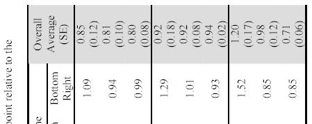
85 64

86 Table 6.4 Ratio of the average aerosol concentrations between the reference and mannequin planes prior to wind tunnel modification, each including 2-4 experimental runs, with standard error (SE). Powder Grade Windspeed (m/s) Ratio SE Ratio SE Ratio SE F F F

87 Table 6.5 Correction factors, applied to the measured reference concentration for establishing the air concentration at the mannequin, to be used for calculating inhalability, for pre-modification experiments only, with standard error (SE). Powder Grade Windspeed (m/s) Ratio SE Ratio SE Ratio SE F F F F * -- * -- *Condition not tested 66

88 Table 6.6 Uniformity of aerosol concentration along the vertical axis of the wind tunnel, across both sampling planes, shown as the average ratio of each sampling location to the center point, with standard error (SE). Powder Grade Windspeed Top Bottom (m/s) Ratio SE Ratio SE F a a a 0.03 F a a a 0.03 F F a a F F a Difference from center is statistically significant at α =

89 Table 6.7 Uniformity between the reference and mannequin planes, as represented by the average concentration ratio for each sampling point on each plane for all powder grades and windspeeds of interest, based on 3 measurements for each plane, with standard error (SE). Powder Grade Windspeed (m/s) Ratio SE Ratio SE Ratio SE F F F F a 0.11 F a F a a Difference between reference and mannequin plane is statistically significant at α =

90 Table 6.8 Correction factors to be applied to the reference sampler measurement of aerosol concentration for the determination of the actual aerosol concentration at the mannequin plane, as measured by the ratio of the center point concentration for each plane, shown with the standard error (SE). Powder Grade Windspeed (m/s) Ratio SE Ratio SE Ratio SE F F F F F F

91 Table 6.9 Particle size distributions measured using modified Marple-type cascade impactors prior to wind tunnel modification, represented by the mass median aerodynamic diameter (MMAD) and geometric standard deviation (σ g ). Powder Windspeed (m/s) Nominal Value Grade MMAD MMAD MMAD MMAD σ (µm) g σ (µm) g σ (µm) g σ (µm) g F F F

92 Table 6.10 Particle size distributions, measured by modified Marple-type cascade impactors, for all powder grades and windspeeds of interest in the fully modified wind tunnel, represented by the mass median aerodynamic diameter (MMAD) and geometric standard deviation (σ g ). Powder Windspeed (m/s) Nominal Value Grade MMAD MMAD MMAD MMAD σ (µm) g σ (µm) g σ (µm) g σ (µm) g F F F F F a 1.19 a F a 1.29 a a Nominal value used for this condition 71

93 Figure 6.1 Conceptual sketch of the new ultra-lowspeed wind tunnel, showing aerosol injection from both overhead and upstream and the resultant particle trajectories. 72

94 Figure 6.2 Fully constructed ultra-lowspeed wind tunnel facility with heated, breathing mannequin installed. 73

95 (a) (b) Figure 6.3 Time-lapse photographs of the windspeed measurement technique, showing several smoke blips as they travel across the section in which they were timed. Also shown are the strings that demarcated the timing section and eliminated the problem of parallax. 74

96 Windspeed (m/s) Pressure Drop ("H 2 O) Figure 6.4 Calibration of pressure drop versus windspeed across the range of wind tunnel operations, shown with one standard deviation. 75

97 Figure 6.5 One of the Topas dust generators used to aerosolize and inject narrowly graded powders of fused alumina into the wind tunnel. 76

98 Figure 6.6 Bi-directional tracking system used to fully disperse aerosols injected into the upstream mixing chamber, with the white arrows indicating the range of motion of the injection nozzle provided by the tracking system and the gray arrow indicating the direction of airflow. 77

99 Figure 6.7 Structure used for wind tunnel calibration measurements, in this case shown with the Marple cascade impactors used to measure particle size distribution, but also used to measure aerosol concentration distribution with IOM samplers facing upwards as static samplers. The gray arrow indicates the direction of airflow. 78

100 Figure 6.8 Modified Marple-type cascade impactor used to measure particle size distributions, shown assembled with the cap (not used here). Also shown is one of the disassembled top foam stages. 79

101 Figure 6.9 New mannequin system shown (a) fully assembled inside the wind tunnel, (b) with the face piece opened to reveal the internal filter holder, and (c) with all peripheral components. 80

102 Figure 6.10 Mannequin breathing machine, consisting of two pneumatic cylinders and a servo-linear actuator that cycles in and out to produce a representative range of human breathing flowrates. 81

103 Figure 6.11 Mannequin breathing manifold with attached filter holder, indicating the various nose and mouth orifices as well as the separate internal tubing connections. 82

104 Chapter 7 VISUALIZATION OF THE FLOW AROUND A BREATHING MANNEQUIN AT ULTRA-LOW WINDSPEEDS In the same way that most of the research on human inhalability has not included the ultra-low windspeeds of interest, characterization of air movements around the human body at low windspeeds has also not been fully studied. On the other hand, laboratory studies have been carried out for higher windspeeds greater than 0.5 m/s looking at external airflow effects around a breathing mannequin. For example, Wood and Birkett (1979) found qualitative evidence of air disturbances resultant from the breathing action of a mannequin operating with a minute volume of 25 L/min at 1 m/s windspeed. However, with respect to personal samplers mounted onto the mannequin lapel, their observations did not translate into quantifiable differences in sampling efficiency. In addition to such experimental work, extensive theoretical or mathematical modeling has also been conducted to understand the physical processes that influence human aspiration (Erdal and Esmen, 1995; Dunnett and Ingham, 1986; and others). More recently, numerical modeling of human aspiration has included computer simulations of airflow patterns around the human body under calm air and ultra-low windspeed conditions (Gilmutdinov and Zivilskii, 2008). However, laboratory experiments examining airflow patterns around a simulated human both breathing and heated have not been attempted in the more relevant ultra-low range of windspeeds. Understanding air movement in the newly developed system, described in Chapter 6, was therefore identified as an important initial segment of the larger body of work characterizing human aspiration at ultra-low windspeeds. In that way, the flow visualization experiments described here were intended as a qualitative analysis of the effect of various physical parameters (e.g., minute volume, 83

105 breathing mode, etc.) on the airflow around a mannequin in low windspeed environments, with the focus on air patterns directly in front of the nose and mouth during human inhalation. These parameters are important because they strongly influence particle transport, and hence the efficiency of inhalation, in that region. The results will therefore complement and provide additional insight to later quantitative experiments of human inhalability in low windspeeds performed under the same conditions, described in following chapters. 7.1 Visualization methods An ideal visible tracer method was sought that would accurately reflect the motion of the air itself and thereby identify the streamlines that define the airflow pattern in the wind tunnel and around the mannequin; such a method would indicate the expected motion of particles within that air stream. The free stream turbulence in the new wind tunnel was low enough that such flow visualization was possible, aided in part by the upstream honeycomb that served to straighten the airflow as it entered the working section. For purposes of the present work, several methods of flow visualization were considered or attempted. Initially, helium bubbles were identified as a potentially simple and nontoxic technique, similar to what has been used by aerodynamicists (Kerho and Bragg, 1994; Mueller, 1996). A commercially available helium bubble generator (Sai, Sage Action, Inc., Freeville, NY, U.S.A.) was set-up outside the wind tunnel, with a stainless steel connecting tube for the introduction of bubbles directly into the working section. In that system, soap bubbles were filled with helium gas such that they remained neutrally buoyant and would, theoretically, follow the airflow inside the wind tunnel. One difficulty that arose with this technique was the fragile nature of the bubbles, which tended to die before they entered the working section of the wind tunnel. This was due in large part to the length of piping that was necessary to introduce the bubbles throughout the entire cross section of the wind tunnel. In addition, the helium bubble generator required very precise adjustment to create an appropriate, uniform bubble size, which was important for establishing and maintaining the desired neutral buoyancy. 84

106 These difficulties in achieving optimum conditions were a significant impediment to the use of this technique in the present research. After many attempts and a considerable amount of time, application of this method continued to prove very challenging and satisfactory results were never fully realized. Another option that was considered, but never carried out, was the hot-wire smoke generator, which has been widely used in other wind tunnel studies for smoke generation purposes (Sreenath et al., 1997). This technique employed a heated wire onto which oil droplets would fall and create lines of smoke. One major drawback to this method, however, was that it would require the construction of housing for the system. That would have been significantly cumbersome inside the wind tunnel and would have severely disturbed the airflow, as would the presence of a heat source inside the wind tunnel. After careful consideration, this option was therefore not attempted. Ultimately, the technique that proved most effective, and so was developed and employed, involved the use of smoke generated from incense sticks. Initially, the lighted sticks were placed directly into the working section of the wind tunnel to generate smoke. Here, however, it was observed that the smoke tended to rise upwards and did not appear to follow the airflow directly. The same phenomenon was also seen when the incense stick was placed further upstream of the working section, i.e., before the honeycomb structure. Rising smoke was also evident when cigarettes were used for smoke generation as well, and so the effect did not appear to be related to the particular incense sticks used. It was believed then that the heat generated from the burning of the incense might have been the cause of that anomaly, which presented a similar problem to what was anticipated for the hot-wire technique. In order to eliminate such effects, the smoke was generated in a chamber located outside the wind tunnel, which proved highly effective. Figure 7.1 depicts the system that was eventually realized. Figure 7.1a shows the external smoke chamber, which was constructed of particleboard on 5 sides with a plexi-glass top and steel brackets holding all sides together. For this study, eight incense sticks (Florasense Incense, Blyth HomeScents International, Des Plaines, IL, U.S.A) were 85

107 lighted and placed inside the chamber and allowed to burn for at least five minutes before turning on the wind tunnel. This allowed for the smoke to accumulate and therefore the smoke lines appeared thicker. In order to introduce smoke into the wind tunnel, tubing was attached from the smoke chamber through the floor of the upstream mixing chamber, as can be seen in Figure 7.1a. Figure 7.1b shows the part of the system that was located inside the wind tunnel, which consisted of a long, rigid plastic tube, measuring approximately 1.2 meters, connected to the end of the flexible tubing. Twelve small, equally spaced holes were drilled into the rigid tube, allowing smoke to enter the wind tunnel as parallel streams. This tube was placed flush against the honeycomb and could be oriented in both the vertical and horizontal directions along any plane of the wind tunnel. For the system described, smoke was drawn into the wind tunnel using only negative pressure by the four fans at the downstream end of the wind tunnel. That eliminated the need for additional forced air to introduce smoke into the wind tunnel, thus ensuring that no secondary airflows were generated from this method. As can be seen in the resultant photographs (see later Figures 7.3 through 7.6), the mannequin body and the space between the mannequin and the wind tunnel floor were sealed with polyurethane film in order to reduce potential leakage of outside air into the working section. Assuming there were no leaks or other unwanted sources of air in the wind tunnel, it was reasonable to expect that the smoke lines generated in the manner just described directly followed the air stream. It should be noted that incense smoke generally has aerosol particle sizes between 0.1 and 1 µm (Yang et al., 2007), which indicated that issues with gravitational settling would not be expected. Although that particle size range is smaller than what will be used for later experiments, incense stick smoke proved to be an excellent technique and enabled clear visualization of the air patterns around the mannequin. In addition, the fully enclosed nature of the smoke chamber and the use of HEPA filters in the wind tunnel limited exposure of the researchers to the smoke. 86

108 A sketch of the wind tunnel configuration ultimately used for the flow visualizations can be seen in Figure 7.2. An important feature of this set-up, as seen in the figure, was the lighting system developed in order to enable adequate illumination of the smoke traces as they moved through the wind tunnel working section. This was achieved by placing a series of five 250-watt floodlight bulbs inside the upper mixing chamber, sitting directly atop the honeycomb structure that separated that chamber from the main exposure section. With the help of the honeycomb, this provided columniation of the light and excellent illumination of the smoke lines and mannequin. As mentioned previously, it was important to limit sources of heat inside the wind tunnel, and therefore the lighting system remained off unless it was required for the purpose of video recording. The primary flow visualization experiments to examine windspeed, breathing flowrate, and mode of breathing were all carried out with the mannequin facing directly into the wind in order to best understand the fundamental impact of those parameters. Those assessments did not take into account the behavior of smoke traces after they had passed the mannequin. As described previously in Chapter 6, the mannequin was attached to a rotational mechanism to obtain orientation-averaged sampling results for the subsequent inhalability and personal sampler studies. That served to eliminate any bias associated with the directionality of an aerosol source, as required for those later studies. For the flow visualization studies then, it was of some interest to understand the patterns of air movement around the mannequin at several angles, covering the range of orientations for which the mannequin would ultimately be sampling. However, it is clear from Figure 7.2 that illumination was primarily upstream of the mannequin. This prevented the capturing of videos that could adequately demonstrate the impact of orientations other than facing directly upstream. Therefore, the analysis of breathing effects at other orientations required the use of a large hand-held flashlight to illuminate the flow in front of the rotated mannequin, with detailed observations subsequently written down; consequently, no videos exist for that analysis Most of the experiments to be described here were also performed with an unclothed mannequin. However, the aerosol experiments described in Chapters 8 and 9 utilized the 87

109 mannequin wearing a laboratory coat onto which personal samplers were mounted. It was therefore important to understand any effects of added garments on the airflow around the mannequin and a limited set of tests were carried out to look at this. Again, full video recordings were not obtained, and so only observations written down at the time of the experiments are discussed. From the outset it was recognized that the usefulness of this flow visualization study would be heavily dependent on obtaining high quality images of the flow patterns around the mannequin. With this in mind, appropriate photography and video equipment was purchased. The new digital camera (Panasonic, DMC-FZ50 Lumix) was capable of producing not only high-resolution photographs, but also high-quality video clips, from which high quality photographs could also be extracted. During the experiments, the camera was placed on a fixed tripod to ensure that the resultant videos had a consistent appearance in terms of scale and background. To help with this, black-out paper was installed on the back wall of the wind tunnel to reduce glare. In addition, thick black cloths were draped over the wind tunnel viewing windows to significantly reduce ambient light. Each of the final videos obtained using this system lasted for approximately 40 seconds and incorporated from 5 to 10 full breathing cycles Experimental conditions The parameters that were modified for the flow visualization experiments are listed in Table 7.1. They were chosen to complement those conditions for which future quantitative inhalability and personal sampler measurements were to be carried out, including: Windspeed (m/s) Breathing flowrate (minute volume, L/min) Mode of breathing (i.e., nose or mouth breathing) Body temperature ( C) 88

110 Orientation Clothing Three different windspeeds (0.10 m/s, 0.24 m/s and 0.42 m/s) were chosen to examine the range of environments that are considered ultra-low. Two different breathing flowrates, expressed in terms of minute volume, were chosen to simulate at rest breathing and a moderate work level (6 L/min and 20 L/min, respectively). Those values were based on either 12 or 20 breaths per minute with either 0.5 L or 1.0 L tidal volume, respectively. The modes of breathing that were used included mouth-only breathing (in and out through the mouth), nose-only breathing (in and out through the nose), and in through the nose but out through the mouth (nose-mouth breathing). The additional possibility of breathing in through the mouth and out through the nose was not included because this was not considered to be a normal mode of breathing. At the higher breathing flowrate (20 L/min), nose-only breathing was not examined because this too was not considered a common breathing pattern 1 (Saibene et al., 1978). Combining the parameters of breathing flowrate and mode of breathing provided 5 different breathing patterns : 6 L/min mouth, 20 L/min mouth, 6 L/min nose, 6 L/min nose-mouth, and 20 L/min nose-mouth. Mannequin body temperature was regulated through a computer-controlled heating mechanism and was either unchanged (i.e., room temperature) or heated to typical human skin temperature (33 ºC). Analysis of orientation effects was completed under a slightly more limited set of conditions, with the mannequin operating unheated with either nose-only or mouthonly breathing for each of the three windspeeds and two flowrates used previously. The orientations that were studied included facing into the wind (0º), at a right angle to the wind direction (90º), and facing downstream from the wind direction (180º). Again to a limited extent, the effects of clothing lab coat, safety glasses and hard hat were tested for the mannequin both heated and unheated but not breathing. 1 The term breathing pattern as used here refers to the various combinations of flowrate and breathing mode, so that ultimately 5 different breathing patterns were examined: mouth-only at 6 L/min, mouth-only at 20 L/min, nose-only at 6 L/min, nose-mouth at 6 L/min and nose-mouth at 20 L/min. 89

111 A complete description of the mannequin breathing system was offered in Chapter 6 and so only important details will be repeated here. It will be remembered that the mannequin was set up with two mouths, one vertically adjacent to the other and each measuring approximately 40 mm by 3 mm, as well as two nostrils, set side by side in the normal human anatomical position, each measuring 12 mm in diameter. The mannequin was created this way in order to prevent inhalation and exhalation from using the same pathway, thus eliminating the potential for re-entrainment of particles collected onto the filter or along the inside walls prior to reaching the filter. For mouth-only breathing, inspiration 2 was therefore through one mouth orifice and expiration through the other. Due to the size of the filter holder located along the inhalation pathway for use during later studies where inhaled aerosols are collected the inhalation tubing was always attached to the upper mouth, with expiration through the lower mouth. Although the present study of air patterns around the breathing mannequin did not require the use of any filters, the same configuration was used here for consistency. Similarly for nose-only breathing, inspiration was through one nostril and expiration was through the other nostril. In this case, each orifice was available for either inspiration or expiration, but again for consistency, inspiration was established always to be through the left nostril with expiration through the right nostril. It is important to acknowledge that in these simulations, the jet produced by breathing through only one nostril, as opposed to normal human breathing through both nostrils at once, was not an entirely accurate picture of real human nasal breathing. However, the size of each nostril was designed such that the air velocity in the expired air jet was the same as would have been achieved for the two nostrils at actual size. It should be noted then that preliminary observations confirmed that no difference in air disturbance was visible based on which nostril was chosen for expiration. 2 The terms inspiration and expiration are used here to describe the act of breathing air without aerosols, i.e., only clean air is being drawn into the nose and/or mouth. The words inhalation and exhalation imply the presence of aerosols. 90

112 Basis for qualitative analysis As previously stated, this portion of the overall body of research was largely qualitative. So a few words are given here to explain the basis upon which these analyses were performed. For each condition of interest, the primary analytical question was: Was the airflow approaching the mannequin noticeably modified by the breathing action of the mannequin? Essentially, this is asking if obvious movements in the smoke near the mannequin nose and/or mouth appeared when it began breathing and disappeared shortly after it stopped breathing. If so, then the next question was: Did the modification persist long enough to disturb the airflow through the subsequent inspiration phase? In other words, did the expired air continuously disturb the airflow in front of the mannequin throughout the entire breathing cycle? If the answer was yes, then it was concluded that such disturbance was large enough to potentially impact aerosol transport during breathing, and by extension affect aspiration efficiency. If the answer was no, then it was concluded that the impact of that air disturbance on inhalability would be negligible. An additional research question that was of interest was the extent to which body temperature might affect air movement around the heated mannequin. In theory, a warm body has the potential to produce secondary air movements, based on the tendency of hot air to rise relative to colder air. The following question was therefore posed: Did smoke traces around the heated mannequin while it was not breathing show any significant, continuous air disturbances near the nose and/or mouth that differed noticeably from that seen for the unheated mannequin? 91

113 If so, then it would be concluded that body temperature could potentially impact aerosol transport as well. 7.2 Results and discussion The ultimate outcome of the flow visualization experiments was a library of videos 30 in total depicting the breathing mannequin under the various sets of conditions specified above. From those, still photographs at various points in the mannequin breathing cycle were extracted and compiled into the figures shown here. These specific examples were chosen for the clarity with which they show the overall results, but the full set of extracted photographs are provided in Appendix A. In each case, the pictures are meant to represent what was observed at the peak of the inspiration and expiration phases. Those points were determined by both visually identifying the moment at which the smoke disturbance was closest to and farthest from the breathing orifice concerned and also by noting the audible sounds also captured in the recordings that accompanied inspiration and expiration. Although the raw video footage was considerably more instructive for analysis, it is obviously not possible to include them here. So the photographs are shown with the understanding that they are representative of the actual video recordings Effect of windspeed Figure 7.3 shows typical results for analyzing the effect of windspeed on air movements around the breathing mannequin in that particular example the photographs were taken with the mannequin unheated and breathing through the mouth at 6 L/min. As seen in the figure, there was a clear difference in airflow disturbances around the mannequin based on the windspeed in the tunnel. Even before the mannequin started to breathe, the undisturbed air looked somewhat different at 0.10 m/s compared to what was observed at 0.24 and 0.42 m/s, specifically in relation to the thickness and smoothness of the smoke lines. At the two higher windspeeds, the smoke lines were less smooth and contained small internal eddies that tended to increase the width of the smoke lines. Some of that 92

114 was due to a slight increase in free stream turbulence present at the higher windspeed, but some was also likely the result of imperfections in the holes drilled into the rigid plastic injection tubing. The results indicated that, during expiration, the lowest air velocity (0.10 m/s) produced a larger area of disturbed air directly in front of the mannequin face compared to the higher air velocities. During inspiration, which is the most important phase in terms of predicting any effects on inhalation measurements, the lowest windspeed still showed a disturbed airflow pattern, resulting from the persistence of the disturbance that was generated during expiration in the preceding cycle. In other words, the original, smooth airflow pattern that existed when the mannequin was not breathing did not fully recover to its previous stable pattern in the lowest windspeed situation. In contrast, at 0.24 m/s and 0.42 m/s the smooth smoke pattern was seen to fully recover by the end of the subsequent inspiration phase. That indicates that at low windspeeds the mannequin s expired air has the potential to impact aerosol inhalation, but at higher windspeeds no impact would be anticipated. As expected, for a given windspeed, the actual degree of disturbance in terms of how far the plume of expired air extended out in front of the mannequin was also dependent on both the mode of breathing and the breathing flowrate. Looking at the collection of videos for each breathing pattern, similar results with regard to the effect of windspeed (i.e., more disturbed flow in the lowest windspeed) were seen for all but one combination of breathing mode and breathing flowrate. That exception was for nose-only breathing at the low flowrate (6 L/min), where the air disturbances were minimal and not persistent for all windspeeds, and therefore no significant effects would be expected. The individual impact of these other factors is discussed in more detail below Effect of breathing flowrate Figure 7.4 shows the effect of breathing flowrate, depicted here by the example of an unheated, mouth-only breathing mannequin at 0.24 m/s windspeed. It was evident that, 93

115 for every combination of windspeed and mode of breathing, the lower flowrate produced a plume of expired air that did not extend upstream as far as that from the higher flowrate. There was also an inverse relationship between the flowrate and the windspeed, such that the least amount of disturbance was observed when the mannequin was breathing at rest in the higher windspeeds. Conversely, the most disturbed air was seen when the mannequin was breathing at the high flowrate in the lowest windspeed. For the same mode of breathing (i.e., for the same inlet diameter), the velocity of the expired air will be different based on the breathing flowrate. The observed difference based on flowrate is therefore not surprising, and would be accounted for by the different combinations of the tidal volume (0.5 versus 1.0 L) and the breaths per minute (12 versus 20). The breathing flowrate should therefore be taken into account as a possible influential factor with respect to human aspiration efficiency Effect of breathing mode Figure 7.5 shows the effect that the mode of breathing had on the airflow around the mannequin. Expiration through the mouth created a jet that was directed into the area immediately in front of the mannequin head for the stationary mannequin used here, that direction was upstream. When the mannequin was expiring through the nose, the jet was instead directed at a downward angle close to the body, disturbing the air in front of the mannequin torso. The condition of inspiration through the nose with expiration through the mouth looked similar to mouth-only breathing, with disturbances in front of the head. This latter observation indicated that it was likely that the expiration process produced the air disturbances seen in the smoke traces, making the inspiration process appear irrelevant with respect to altering air patterns around the mannequin. On the other hand, the disturbance from mouth-only breathing was always greater than that from nose-only breathing. So, for the case of nose-mouth breathing it is hard to understand the relative impact of each orifice and it is therefore difficult to predict from this qualitative analysis 94

116 alone if differences in the mode of inspiration might indeed influence aerosol transport and inhalability. Overall, however, it was clear that, at the same breathing flowrate, the air was more highly disturbed when mannequin expiration was through the mouth. Another consideration with respect to nose versus mouth breathing relates to personal samplers mounted onto the body. The observed differences in the direction of the expired air jet for nose and mouth breathing could potentially produce discrepancies in sampler measurements and sampling efficiency. Specifically, exhaling through the nose might alter the concentration of aerosols in the vicinity of the samplers to a greater extent than exhaling through the mouth. By extension, that may impact the relationship between sampler and mannequin measurements in the experiments that will be described later Effect of body temperature Figure 7.6 shows examples of the effect that body temperature had on airflow patterns around the non-breathing mannequin at different windspeeds. For the two higher windspeeds (0.24 and 0.42 m/s), there was no noticeable impact from heating the mannequin to skin temperature. At the lowest windspeed (0.10 m/s), however, a comparison of the smoke patterns around the heated and unheated mannequin indicated an interesting phenomenon in which the smoke appeared to be forced downward. In other words, when the mannequin was unheated all the smoke lines stayed at the same height level at which they entered the working section, but when the mannequin was heated and in extremely low windspeeds, the uppermost smoke lines traveled at a downward angle towards the mannequin. Specifically, the topmost smoke line, which entered the wind tunnel only a few inches below the top of the working section, subsequently reached the mannequin at the level of its head, approximately 30 cm from the wind tunnel ceiling. While interesting in its own right, this observance did not actually disrupt the airflow in the immediate vicinity of the mannequin nose and mouth, and therefore it is not likely to influence aerosol inhalability or personal sampler performance. 95

117 One explanation for this observance is a buoyancy effect, whereby air that had risen off the heated mannequin collided with the wind tunnel ceiling to create a re-circulating eddy in the upper portion of the chamber; that in turn may have served to deflect the incoming smoke. Additional support for this explanation can be seen in a wave-like pattern that was also observed in the upper levels of smoke under those conditions. In such a scenario, the confined space of the wind tunnel appeared to be a key, mitigating factor, and observance of the same phenomenon would not be likely to occur in a larger wind tunnel facility or as it relates to practical situations in an unconfined open space. Again, this phenomenon was observed at the lowest windspeed only, and the effect of body heat was clearly insignificant at the higher windspeeds Effect of body orientation As mentioned previously, assessment of the possible impact of other orientations required visualization of the smoke downstream of the mannequin. Due to the complex flow around the mannequin body, including associated flow separation and turbulence, it was not possible to obtain video recordings of sufficient quality. Therefore, the results described here are based on written observations made at the time of the experiments. It was seen that turning the mannequin to a 90 angle, facing towards the side wall of the wind tunnel, affected the smoke patterns only slightly, and in a way such that no impact on aspiration efficiency would be expected. Eddies were observed on the downstream side of the head as a result of separation of the air flowing over the mannequin and recirculating against the body. These secondary air movements were clearly not a result of the mannequin breathing action, although they did appear to be close enough to the nose and mouth that aerosol inhalation might potentially be affected. Other than this possibility, the breathing action itself did not alter the smoke in ways noticeably different from what was previously observed for the conditions tested here. At 180º, facing downstream into the wind tunnel, the smoke pattern at the mannequin face was seen to be highly disturbed due to the same eddy formation just described. 96

118 These eddies were closest to the mannequin face at the lowest windspeed, with increasing windspeed creating more distance between the smoke eddies and the nose and mouth. The same patterns of smoke disturbance that resulted from the breathing patterns of the forward-facing mannequin (e.g., mouth breathing extending out from the face and nose breathing directed at a downward angle, etc) were similarly evident at this orientation. However, one difference that was observed was that nose-only breathing appeared to generate smaller disturbances in front of the mannequin torso relative to the 0 upstream orientation. That was most likely the result of airflow blockage by the mannequin body, as evidenced by a lack of smoke in that region. It should also be noted that, because the mannequin will be rotating continuously throughout the following inhalability experiments, those results will be averaged over all orientations and any impact that different body positions may have had would be negated Effect of clothing and personal protective equipment The presence of all three garments lab coat, safety glasses, hard hat did not impact the movement of smoke around the unheated mannequin in any significant way. The tracer lines did appear to travel over the hard hat more aerodynamically, but overall the same air disturbances were observed as before and no additional ones were noted. The glasses and lab coat did not appear to have any significant effect as well. It should be noted however that when the mannequin was heated to skin temperature, the presence of the lab coat and hard hat had a slight cooling effect such that the garments displayed a lower temperature than the mannequin body itself, as measured by an infrared thermometer. It is possible then that the presence of such clothing might reduce or eliminate the phenomenon observed in the airflow around the heated mannequin at the lowest windspeed. 7.3 Conclusions Table 7.2 shows an integrated summary of these findings, indicating the conditions for which the impact of expired air was substantial enough to noticeably and continuously destabilize the air upstream of the mannequin. In other words, for those conditions 97

119 indicated in the figure, expiration from the mannequin permanently disturbed the surrounding airflow throughout the entire breathing cycle and smooth smoke lines were never re-established. It was apparent that the lowest windspeed tested here (0.10 m/s) showed a markedly different airflow pattern than the highest windspeed for nearly all conditions of interest. In addition, the higher flowrate (20 L/min), representative of a moderate working level, tended to show more extensive disturbances to the approaching air compared to at rest breathing (6 L/min). And finally, expiration through the mouth was clearly more disruptive to the approaching air stream than expiration through the nose, for which the primary disturbance was in front of the torso and was not persistent. It should also be reiterated that body temperature, orientation and clothing did not show any significant effects that might present a concern for future measurements of inhalability. Although this study was focused on the impact that mannequin expiration had on airflow in the wind tunnel, these results provide an interesting insight about the impact that the route of inspiration (i.e. nose versus mouth) might have on aerosol transport in the vicinity of the breathing orifice. For the case where the mannequin was breathing in through the nose and out through the mouth, the smoke patterns were identical to those seen for mouth only breathing, regardless of the breathing flowrate. That indicated that it was the force of the expired air projecting out of the body, not the force of air being inhaled into the body, which led to the air disturbances seen in the videos. If the rate of airflow into and out of the nose and/or mouth was the same, as governed by the moving pistons of the breathing machine, the larger diameter of the nose will produce an inlet velocity that is smaller than that from the mouth. It therefore makes sense that exhaling through the mouth will produce a more forceful air jet. Ultimately, this may result in differences in measured aspiration efficiency based on the mode of breathing. Of course, a full understanding of these observed differences will require the future quantitative measurements of inhalability obtained at the same experimental conditions. As mentioned above, the placement of personal samplers on the body of the mannequin might also be affected differently by different breathing parameters the downward trajectory of aerosols resultant from nose-only breathing could potentially impact the 98

120 concentration collected by such samplers. But again, the expired air jet from the nose was relatively weak compared to that from the mouth, and so any impact on sampling efficiency may not be detectable. Those concepts will be important to consider when comparing data from personal samplers mounted onto the mannequin operating under different breathing conditions, described in Chapter 9. To varying degrees, each of the parameters that were found to be important windspeed, breathing flowrate and mode of expiration have the potential to impact the accumulation of particles near the mannequin face and therefore may influence measurements of aerosol inhalation. Of course it is not possible from these videos alone to determine the direction an increase or decrease in aspiration efficiency in which these results might show an effect, if in fact the effects are quantifiable at all. Whether or not any of these observed differences holds true in actual practice will be studied in the quantitative inhalability experiments described in Chapter 8. On the whole, these flow visualizations enable the recognition of those scenarios for which possible effects are most likely to influence aerosol transport as it relates to inhalation. Ultimately, the importance of qualitative understanding of the airflow patterns around this life-sized mannequin will be useful for analyzing the quantitative measurement of human inhalability provided by the same mannequin. 99

121 Table 7.1 Parameters modified for flow visualization experiments. Breathing Body Orientation Windspeed Mode of Flowrate Temperature (º From wind (m/s) Breathing (L/min) (ºC) direction) Clothing 0.10 Mouth Lab coat 0.24 Nose 20 Ambient (~23) 90 Hard hat 0.42 Nose-Mouth 180 Safety glasses 100

122 Table 7.2 Summary of results from all flow visualizations, indicating those conditions for which significant disturbances were noted ( YES ) and where no effects were observed ( NO ). Breathing Windspeed (m/s) Parameter Mouth 6 L/min YES NO NO 20 L/min YES YES NO Nose 6 L/min NO NO NO Nose-Mouth 6 L/min YES NO NO 20 L/min YES YES NO 101

123 (a) (b) Figure 7.1 Smoke generating equipment for flow visualization studies, including (a) remote smoke chamber with flexible tubing connection and (b) rigid plastic tube for ultimate dispersal into wind tunnel working section. 102

124 Figure 7.2 Wind tunnel set-up for smoke generation and flow visualization. 103

125 Figure 7.3 Still photographs extracted from flow visualization videos depicting the air disturbances in front of an unheated mannequin, breathing through the mouth only at 6 L/min, in windspeeds of (a) 0.10 m/s, (b) 0.24 m/s and (c) 0.42 m/s. 104

126 Figure 7.4 Still photographs extracted from flow visualization videos depicting the air disturbances in front of an unheated mannequin, breathing through the mouth only, at 0.24 m/s, for breathing flowrates of (a) 6 L/min and (b) 20 L/min. 105

127 Figure 7.5 Still photographs extracted from flow visualization videos depicting the air disturbances in front of an unheated mannequin at 0.24 m/s windspeed, breathing at a flowrate of 6 L/min using (a) nose-only, (b) mouth-only and (c) nose-mouth breathing. 106

128 Figure 7.6 Still photographs extracted from flow visualization videos depicting the nonbreathing mannequin, both heated and unheated, at external windspeeds of (a) 0.10 m/s, (b) 0.24 m/s and (c) 0.42 m/s. 107

129 Chapter 8 ASPIRATION EFFICIENCY OF A BREATHING MANNEQUIN AT ULTRA-LOW WINDSPEEDS With the new ultra-lowspeed wind tunnel fully calibrated (see Chapter 6) and the flow patterns around the heated, breathing mannequin examined (see Chapter 7) measurements of mannequin aspiration efficiency were then possible. This chapter will therefore describe the primary experiments carried out to assess human inhalability at ultra-low windspeeds. Firstly, the new data were examined with respect to the factors potentially influencing aspiration efficiency, including particle size, windspeed and the various mannequin breathing parameters. Next, the data were looked at in light of the potentially influential physical processes outlined in Chapter 5, including the development of a model based on the dimensionless quantities discussed there. Discussions will also include reference to the flow visualizations from the preceding chapter and how those results may provide additional insight into these quantitative measurements. Ultimately, these discussions will help form a more complete understanding of human aspiration efficiency at the ultra-low windspeeds of interest. 8.1 Experimental methods The experimental methods employed here involved measuring the aerosol concentration inhaled by a breathing mannequin and relating it to the aerosol concentration measured by a reference sampler. The new ultra-lowspeed wind tunnel and heated, breathing mannequin, previously described in Chapter 6, form the primary experimental set-up for assessing the aspiration efficiency of the human head in ultra-low windspeed environments. The mannequin was located in the center of the wind tunnel working section, approximately 1.5 meters downstream of the forward mixing chamber. It was connected to a remote computer that controlled both the heating and breathing elements, 108

130 with internal wires fed through the floor of the wind tunnel via the center shaft of the rotating mechanism on which the mannequin sat. For each experiment, a 47-mm glass fiber filter was conditioned overnight in a desiccator to stabilize the mass by reducing the moisture content then weighed and inserted into the filter holder. The entire device was then snapped into place along the inhalation pathway inside the mannequin head. Tweezers were used to transfer the filters into and out of the holder and powder-free latex gloves were also worn to reduce contamination. The filters were analyzed gravimetrically using an electronic analytical balance (Model MC210S, Sartorius, Elk Grove, IL, U.S.A.) located in a room adjacent to where the wind tunnel was operating. After sampling, the entire filter holder was removed from inside the mannequin head for transport to the balance room, being careful to keep the inlet pointed upward so as not to lose any of the sample. The conical cover piece of the filter holder was set aside for wipe sampling and the filter was removed and placed in a covered glass dish inside the desiccator, to be conditioned again and re-weighed the next day. Any particulate material that was deposited inside the conical piece including on the O- ring was collected using small cotton balls impregnated with isopropyl alcohol. These were similarly conditioned and weighed when thoroughly dry prior to and after sampling. The mass stability of the cotton balls was shown to be comparable to that for the glass fiber filters when similarly allowed to stabilize in a desiccator for at least 24 hours. Finally, particles deposited inside of the mannequin head, along the inhalation pathway between the entry (i.e., the nose or mouth opening) and the filter, were recovered and weighed as well. That was accomplished by pushing the same alcoholenriched cotton balls through the orifice of inhalation using tweezers, being careful to wipe all surfaces along the pathway. Filter and cotton blanks were prepared once each day, typically during the first experiment of that day. Since the filter holder inside the mannequin was the only one of its type, during the experiments, the filter blank was put into a covered glass dish similar to what the loaded filters were placed in after sampling. The cotton blanks were also 109

131 placed into glass dishes after being dipped into the isopropyl alcohol in a similar manner as the cotton balls used for sampling. However, it was not expected that issues related to moisture build-up might arise because, as previously mentioned, they were dried in a desiccator both before and after sampling. In addition, the samples were only transferred approximately 20 meters between sampling and analysis (i.e., from the wind tunnel to the balance) and so sample loss or gain during transport was considered to be minimal. If any of the blanks were questionable or unusable another group was set-up for a later experiment. Ultimately, all reported values were blank-corrected, which meant that differences in the weight of the filter blank or cotton blank were subtracted from the corresponding loaded substrates. The mass of particulates collected (i.e., inhaled) during sampling including the portion recovered by the cotton balls afterwards was obtained by taking the difference in the mass of the filter before and after sampling, and similarly for the cotton balls. The resultant filter (m F ) and wall (m w ) particulate masses were combined minus the resultant masses on the filter blank (b F ) and cotton blank (b c ) to provide the total inhaled aerosol mass. From the breathing flowrate (Q), i.e., the minute volume, expressed as [L/min], and the sampling time (t), the corresponding total volume of inhaled air (V) was calculated: V = Q t (8.1) The inhaled aerosol mass concentration (C M ) was then obtained directly using the following equation: C M ( mf bf ) + ( mw bc ) = (8.2) V An additional important consideration was obtaining an accurate measurement of the true aerosol concentration in the wind tunnel to be used as a reference concentration for calculating inhalability. The best method for this was an isokinetic sampler defined fully in Chapter 5 where the sampler inlet velocity exactly matched the air stream 110

132 velocity. That ensured there was no aerodynamic deflection of particles, such that the result was a measurement of the actual air concentration. For fast moving air (i.e., U > 0.5 m/s), isokinetic sampling is straightforward because convective inertial forces alone largely govern particle motion. On the other hand, for situations where the free stream air velocity is effectively zero (i.e., U < 0.05 m/s), isokinetic sampling in the traditional sense was previously considered inappropriate because vertical movement of particles due to gravitational settling is the primary motion of the particles. In the intermediate range of windspeeds used here, the use of isokinetic sampling therefore had to be carefully considered. Ultimately, it was determined that, despite the additional influence of gravitational settling at low yet, still non-zero windspeeds, isokinetic sampling was still possible based on the same principles governing dispersion of aerosols into the wind tunnel. It was expected that the stream of air eventually aspirated by the isokinetic sampler would experience some loss of particles due to gravitational settling, but that loss would be simultaneously and equally compensated for by particles falling into the aspirated air from above. One anticipated result of this would be enhanced deposition of particles onto the inside walls of the reference sampler. So, such losses were subsequently analyzed along with the filter. As required for isokinetic sampling, the device used here, shown in Figure 8.1, was a thin-walled cylindrical tube, with a plastic conical piece fit over the probe to improve the aerodynamics around the sampler. For the current situation, where the desired inlet velocity (U S ) would be equal to the windspeed (U), the following equation was used to calculate the appropriate flowrate (Q) for each individual windspeed scenario: 2 U Q= πδ S (8.3) 4 where δ = 0.01 m for the reference sampler used here. Although a full assessment of the windspeed inside the wind tunnel was initially performed for calibration purposes, as 111

133 described in Chapter 6, windspeeds were measured again for these experiments to ensure an accurate calculation of the required flowrates. It was then determined that pump flowrates of 0.51, 1.03 and 1.65 L/min were required for the reference samplers at the corresponding nominal windspeeds of 0.10, 0.24 and 0.42 m/s, respectively. For these relatively low required flowrates it was possible to use a personal sampling pump (Model XR5000, SKC Inc, Eighty Four, PA, U.S.A.) to create the desired inlet velocity for the isokinetic samplers. The reference sampler pump was calibrated using a primary flow meter (DryCal DC-Lite, Model 20k rev 1.06, BIOS International), both before each test and then again after sampling was completed. The average of these two values was used to determine the total volume of air sampled. If the change in flowrate throughout an experiment was greater than 5% as per manufacturer recommendations then the sample was deemed unusable and the experiment was repeated. In addition, the pump was programmed with a delay so that before sampling began there was ample time to turn on the wind tunnel, the aerosol generating systems including approximately one minute for the aerosols to properly mix and disperse into the working section and the mannequin breathing machine. In that way, the reference sampler was operating during exactly the same time period as the mannequin. The reference sampler was placed approximately 0.75 meters upstream of the mannequin, a distance close enough to ensure similar aerosol exposure and yet far enough so that any mannequin breathing disturbances would not impact airflow at the reference sampler. Due to do the length of the probe and the expectation of internal wall deposits, alcoholsoaked cotton was used to recover any particles that deposited before reaching the filter. The cotton was handled in the same manner as that for deposits in the mannequin head, i.e., it was allowed to sit in the desiccator overnight before weighing, both prior to and after sampling. In order to get the most accurate estimate of the wind tunnel aerosol concentration at the mannequin itself, a correction factor (a) was applied to the concentration collected at the reference sampler based on the previous determination of the concentration ratio between the two planes, as discussed in Chapter 6 (see Table 6.8). The true reference sampler concentration (C R ) was thus calculated as follows: 112

134 C R ( mf bf ) + ( mw bc ) = a (8.4) V where m F refers to the mass collected on the reference sampler filter, b F refers to the blank filter weight, m w refers to the mass recovered from inside the reference sampler walls, b c refers to the blank cotton weight and V is the volume of air sampled, calculated as before. From Equations (8.2) and (8.4), it was a simple matter to then calculate the mannequin aspiration efficiency or inhalability (A) by taking the ratio of the mannequin concentration (C M ) to the reference concentration (C R ) as follows: C C M A= (8.5) R The nature of the sampling environment and the range of aerosol particle sizes of interest required that slightly different experimental set-ups be used for each combination of windspeed and powder grade. As discussed in Chapter 6, the relationship between the external windspeed and the particle settling velocity necessitated a different proportion of aerosols be injected in each mixing chamber to optimize the spatial uniformity of aerosol concentration and particle size distribution. Aerosols were thus introduced into the test section of the wind tunnel at a range of injection mass flowrates from both upstream and above (see Table 6.2). Each sampling run lasted for 20 minutes and consisted of the breathing mannequin, heated up to body temperature (33 ºC) and dressed in a laboratory coat, with the reference sampler located 0.75 meters upstream. Each experiment included a combination of three different parameters: windspeed (0.10, 0.24 and 0.42 m/s), particle size (as given by the calculated MMAD for powder grades F1200, F800, F500, F400, F280 and F240, representing a particle size range from 9.3 µm up to 89.5 µm), and breathing pattern (6 L/min mouth, 20 L/min mouth, 6 L/min nose, 6 L/min nose-mouth and 20 L/min nose- 113

135 mouth). Two or three tests were performed for each combination of conditions for a total of 183 experiments. As mentioned in Chapter 6, a limited set of preliminary experiments was carried out prior to modification of the wind tunnel. The ranges of conditions at which those were performed included combinations of the three finest powder grades (F1200, F800 and F500) at the same three windspeeds (0.10, m/s), essentially representing 9 particle sizes from about 7 µm up to about 28 µm. For these tests, the mannequin was always breathing through the mouth at 20 L/min. Additional tests were performed for powder grade F500 (representing MMAD of 13.9, 18.6 and 27.9, depending on the windspeed) with the mannequin breathing through the mouth at 6 L/min at all three windspeeds, and also for powder grade F240 (MMAD = 89.5 µm) breathing through the mouth at 20 L/min at 0.10 m/s windspeed only. In those early tests, all aerosols were injected upstream for the three smaller aerosol particle sizes and were injected only from above for the largest aerosol particle sizes. Otherwise, the procedure was the same as for the later full set of experiments. These preliminary tests represented 26 experiments and are included here for completeness, for a total of 209 experiments. The analyses that are described below were performed using SAS 9.1 (SAS Institute, Cary, NC, U.S.A.) and Sigma Plot 2000 (SPSS, Inc., Chicago, IL, U.S.A.). 8.2 Pre-modification versus post-modification experiments Before a full analysis of the data could be undertaken, it was essential to compare the results obtained before and after the wind tunnel was modified. As discussed in Chapter 6, the elutriation of larger particles in the upstream honeycomb required a modification to the wind tunnel in order to test the full set of conditions of interest. Prior to this change, preliminary experiments were carried out to assess the aspiration efficiency of the mannequin for the subset of the desired conditions listed above. It is important to know how inhalability measurements compare before and after the modification in order to establish that the major calibration performed was still valid for the post-modification 114

136 experimental set-up. Additionally, the flow visualizations discussed in Chapter 7 were performed prior to modification and so any utilization of those results as they relate to inhalability required that the airflow not be substantially different after modification. Analysis of the pre-modification results as they compare to the post-modification results was therefore an important bridge that enabled linkage between both the flow visualizations and the wind tunnel calibrations to the full set of inhalability data at ultralow windspeeds. Table 8.1 shows the mean aspiration efficiency results from both before and after the wind tunnel modification, indicating the similar experimental conditions used. Figure 8.2 compares the pre-modification results to the post-modification results, represented by the aspiration efficiency at each corresponding condition for which there are data under both experimental configurations. The solid line represents an idealized relationship with perfect agreement (slope = 1) and the dashed line represents the actual relationship (slope = 0.88). In general, it can be seen that, the aspiration efficiency indicated by the premodification results was somewhat larger compared to the post-modification results for the same sampling environment. One explanation for this is that the elutriation of larger particles into the honeycomb structure shifted the particle size distribution in the working section towards the smaller aerosols. Based on what we already know about the general trend of aspiration efficiency as a function of particle size (i.e., that it increases with decreasing particle size), the smaller particle size distribution in the pre-modification setup would therefore be expected to show higher values for aspiration efficiency. However, a paired t-test was carried out to assess the magnitude of this observed difference and no statistically significant difference between these two sets of data was detected (p-value = 0.214). This provided support for the inclusion of the pre-modification data in the ultimate analyses. Therefore, although those initial data were limited in their scope, they were shown to be broadly consistent with later measurements and so are included in all subsequent discussions. 115

137 8.3 Results The research conducted here represents an important set of experiments that will bridge the gap between the previous aspiration efficiency studies conducted at high windspeeds in traditional wind tunnels and those performed at essentially zero windspeed in calm air aerosol chambers. The data set is therefore presented in its entirety in Appendix B, including experiments performed prior to wind tunnel modification (shown there in shaded rows). A single outlier (A = 2.73) was observed that did not appear to belong to the larger distribution of data points. Ultimately, it was decided not to include this point in data analyses. The particle aerodynamic diameter (d ae ) used for analysis was that value obtained directly from the cascade impactor measurements described in Chapter 6, expressed as mass median aerodynamic diameter (MMAD). Aspiration efficiency was calculated based on the relative concentration between the mannequin and the reference sampler, with the appropriate correction factor applied, as discussed above. All data are displayed graphically in Figure 8.3 for aspiration efficiency (A) as a function of particle aerodynamic diameter (d ae ). Here the graph encompasses the entire set of raw data, including experimental results obtained before the wind tunnel was modified, but excludes the one outlier mentioned. This figure was included to visualize the overall spread of the data, but differences in experimental parameters preclude the calculation of meaningful descriptions of variability there. For that purpose, Tables 8.2 through 8.6 display the mean aspiration efficiency for each of the 18 combinations of windspeed and powder grade under each of the 5 individual breathing conditions: 6 L/min mouth, 20 L/min mouth, 6 L/min nose, 6 L/min nose-mouth and 20 L/min nose-mouth, respectively. Averages include between 2 and 6 repeats except for the noted exception in Table 8.1 for which the outlier was removed. To complement that, Figures 8.4 through 8.8 present graphical depictions of the data. Each point on the graph represents the average of all repeat experiments done under the same conditions, with error bars in the vertical axis showing one standard deviation (SD). For each set of unique experimental conditions, straight lines were drawn between adjacent points to better delineate between the data points at each windspeed. 116

138 A 3-way ANOVA was carried out that looked at the mannequin aspiration efficiency as a function of particle size, windspeed and breathing pattern. The overall interaction model was highly significant (p-value < ), with those three factors explaining 58% of the variability. Each individual variable was also found to be significant (p-value <0.0001, , and , respectively). The next few results sections provide an examination of each of these parameters as directly tested in these experiments. The subsequent discussion section sets about to understand how these parameters interact into various dimensionless groups, as discussed in Chapter 5. That involves a discussion of the physical processes relevant to human inhalability at ultra-low windspeeds, including a new semi-empirical model developed for these data Particle aerodynamic diameter The first parameter that will be analyzed in more detail is the effect of aerosol particle size. As mentioned previously, it is described here by the mass medium aerodynamic diameter (MMAD) and the geometric standard deviation (σ g ) obtained from modified Marple-type cascade impactors (see Tables 6.9 and 6.10). Including the pre-modification data, the size range of the particles tested in these experiments was from 6.8 to 89.5 µm, covering a significant portion of the inhalable aerosol size fraction. These values for aerodynamic diameter were measured directly and most indicated a slight shift upward from the nominal values as determined by Mark et al. (1985). The fact that each combination of powder grade and windspeed constituted a different MMAD and σ g meant that effectively, 9 different particle sizes were tested before modification and 18 different particle sizes were tested after modification. Figure 8.9 shows the mean aspiration efficiency as a function of particle aerodynamic diameter, averaged across all tests performed at each particle size. It will be remembered from Chapter 6 that the powders used for these experiments are narrowly graded, but not monodisperse. Therefore, the particle size value shown on the X-axis is, in actuality, the mass median value from a particle size distribution, the spread of which is described by the geometric standard deviation. In this way, conventional arithmetic standard deviations 117

139 are not appropriate for showing variability. Hence, the horizontal error bars shown in Figure 8.9 represent the 16 th (d 16 ) and 84 th (d 84 ) percentiles calculated from the geometric standard deviation as follows: d50 d16 = (8.6) σ g d 84 = d 50 σ g (8.7) where d 50 represents the mass median aerodynamic diameter (MMAD) and σ g represents the geometric standard deviation. It should also be noted that one would expect additional trends or biases to exist within these data that might also influence human inhalability, related to changes in other experimental conditions, such as windspeed or breathing pattern. Therefore, error estimates for the mean aspiration efficiency on the vertical axis are not appropriate. The effect of these other parameters will be discussed in further detail below. For the entire set of data presented here, ANOVA results showed that particle size was highly significant (p-value < ), with the values for aspiration efficiency generally decreasing with increasing particle size. It is interesting to observe that the general trend for aspiration efficiency as a function of particle size also appeared to agree with the accepted inhalability criterion, as can be observed in Figure 8.9. Here, it can be seen that aspiration efficiency approached unity for the smallest particles and decreased as particle size increased, leveling off at about A = 0.50 for the largest particle sizes. More detailed discussion of the new data presented here as it relates to inhalability criteria and standards will be given in Chapter Windspeed It will now be instructive to further separate out the data into the various experimental conditions to examine the importance of the other parameters tested, which also enables 118

140 the inclusion of variability estimates. The first of these, and a primary topic for this research, was the effect that windspeed had on mannequin aspiration efficiency. Figure 8.10 shows the complete set of data, again represented by the mean aspiration efficiency (A) at each aerodynamic particle size (d ae ), but here it is separated out by windspeed. All breathing flowrates and modes of breathing are included in these means so again it was inappropriate to assign an error estimate. For an indication of the variability, Figure 8.11 shows the results for A as a function of d ae at 0.10, 0.24 and 0.42 m/s, respectively, with data separated into the five mannequin breathing conditions (e.g., 6 L/min mouth breathing, etc) and error bars in the vertical axis showing one standard deviation. The results illustrate that inhalability at lower windspeeds, irrespective of the mannequin s breathing pattern, was consistently greater than at higher windspeeds. ANOVA results for windspeed confirm that aspiration efficiency was significantly greater at 0.10 m/s compared to 0.24 m/s and 0.42 m/s, and was also significantly greater at 0.24 m/s than at 0.42 m/s (all p-values < ). On first inspection of Figure 8.11, it also appeared that the mean aspiration efficiency at 0.10 m/s was generally above the current convention, while at 0.24 m/s the data look relatively evenly distributed about that curve and at 0.42 m/s the majority of values are below it. A more thorough analysis of these data with respect to this criterion is given in Chapter 10, when discussion of the research turns to the relevant standards. Referring back to Figures 8.3 to 8.7, it is also useful to look more closely at the effect of windspeed within each breathing pattern separately, especially since the relationship between windspeed and mean inlet velocity may be influential, as explained in Chapter 5 and discussed in more detail later. The only condition for which windspeed was not a significant factor was with 6 L/min nose-mouth breathing (p-value = ). For all other breathing conditions, aspiration efficiency was significantly different based on windspeed (for a significance level of α = 0.05), with the lowest windspeed always being associated with the highest inhalability. 119

141 8.3.3 Breathing parameters The next parameters of interest all relate to the various mannequin breathing conditions. Looking at the impact of breathing flowrate and mode of breathing as separate parameters is important, but first it will be instructive to look at the combination of those parameters into the five different breathing patterns tested. As previously stated, that included mouth breathing at 6 L/min and 20 L/min, nose breathing at 6 L/min and nosemouth breathing at 6 L/min and 20 L/min. ANOVA showed that aspiration efficiency was significantly different based on the breathing pattern of the mannequin across all windspeeds (p-value = ). However, looking at each windspeed separately (see Figure 8.11), there were no significant differences for aspiration efficiency based on the mannequin breathing pattern at windspeeds 0.10 m/s and 0.24 m/s (p-values = and , respectively), but it did become significant at 0.42 m/s (p-value = ). That apparent dependence on windspeed suggests that the combination of windspeed and breathing pattern may actually be most important to consider, a concept that will be looked at in more detail later with respect to the dimensionless physical parameters. Next, the individual impact of breathing flowrate and mode of breathing were analyzed including differentiation between the inlet and outlet orifices. A 2-way ANOVA was performed to look at these effects, as well as their interaction, which showed that while flowrate was not significant (p-value = ), mode of breathing (p-value = ) and the interaction between the two parameters (p-value = ) were significant factors for determining aspiration efficiency. In order to more fully understand the effect of each breathing parameter individually (i.e., breathing flowrate, inlet orifice and outlet orifice), t-test comparisons between each breathing pattern were carried out, the results of which are shown in Table 8.7. That indicated that mouth breathing at 6 L/min was not significantly different from mouth breathing at 20 L/min, and also nose-mouth breathing at 6 L/min was not significantly different from nose-mouth breathing at 20 L/min. This supports the finding that breathing flowrate by itself was not an important factor for determining inhalability. 120

142 Looking next at the breathing mode, a direct comparison of mouth-only breathing to nose-only breathing suggested that, at the same breathing flowrate in this case, 6 L/min breathing mode was not an important factor for determining inhalability (p-value = ). That is in contrast to the ANOVA results discussed previously, which indicated that mode of breathing was significant across all experiments. In order to understand this further, it may be instructive to look at the relative importance of the separate inhalation and exhalation orifices as they relate to inhalability. This is possible here because different orifices for inhalation and exhalation were used for some tests. In that case, it is interesting to note that mouth breathing at 6 L/min was significantly different from nose-mouth breathing at 6 L/min. However, the same was not true for 20 L/min mouth breathing, which was not significantly different from nose-mouth breathing at 20 L/min. On one hand, that leaves it ambiguous as to the influence that the orifice of inhalation (i.e., inhaling through the mouth versus inhaling through the nose) may have on inhalability. On the other hand, it was shown previously that the interaction of flowrate and mode of breathing was significant. Therefore, it is not surprising that different flowrates might show different levels of importance for the orifice of inhalation as it relates to aspiration efficiency. In contrast, with respect to the orifice of exhalation, for the same breathing flowrate of 6 L/min, nose breathing was not significantly different from nose-mouth breathing. That suggests that the orifice of exhalation was not an important factor for determining inhalability. In fact, across all experiments, the inlet orifice was shown to be statistically significant (p-value = ), with mouth breathing consistently indicating higher inhalability, while the orifice of exhalation was not significant (p-value = ). Finally, it is also interesting to note that the most significant difference was between mouth breathing at 6 L/min and nose-mouth breathing at 20 L/min, which again suggests that the combination of differences in breathing flowrate and inhalation orifice was the most important breathing parameter for determining inhalability. Essentially, the sampling inlet velocity includes mathematically the combination of flowrate and inhalation orifice, shown to be important here. Combining that with the 121

143 apparent effect of windspeed as it related to the breathing patterns of the mannequin, it will be interesting to examine the relationship of the combination of these parameters into the dimensionless quantities that describe the physical principles governing aspiration efficiency. 8.4 Discussion From the preceding results, the discussion will now move into an examination of human aspiration efficiency at ultra-low windspeeds in light of what is already known about the physical principles that govern the sampling and human aspiration of aerosols. It will be remembered that the following function was developed in Chapter 5 for describing aspiration efficiency at ultra-low windspeeds: A = f {St, R, r, B, Θ, Fr} (8.8) These parameters, as defined previously, reflect dimensionless combinations of the various relevant factors already discussed individually e.g., particle size, windspeed, breathing flowrate and mode of breathing. Therefore, examining these parameters may enable a further understanding of the results, and by discerning their relative importance a simplified model may also be developed. Additionally, the results of the flow visualizations described in Chapter 7 will be discussed in terms of how those qualitative findings might help explain the quantitative measurements of inhalability obtained here Stokes number at ultra-low windspeeds Firstly, it is useful to calculate the Stokes number (St) for each experimental condition to examine its importance relative to aspiration efficiency. Table 8.8 lists the relevant Stokes numbers, based on windspeed, particle size, and sampler orifice diameter as defined in Chapter 5, with the mouth and nose having different sampler dimensions of meters and meters, respectively. Figure 8.12 then displays the entire set of raw data for aspiration efficiency (A) as a function of Stokes number (St). What quickly 122

144 emerges is the impact that the different pathways of inhalation (i.e., nose versus mouth) have on the value of Stokes number. In the facility used for this research, the mannequin nose measured 4 times as wide as the mouth, resulting in lower Stokes numbers for nose breathing. Essentially, Stokes number describes particle inertial behavior, with aspiration efficiency of airborne particles consistently shown to decrease as Stokes number increases (Grinshpun et al., 1989 and others). As mathematically defined, Stokes number will increase with increasing windspeed (U), increasing particle size (d ae ), and decreasing orifice diameter (δ). Based on the knowledge of both these well-established relationships (i.e., A decreasing with increasing St; and St increasing with increasing U, increasing d ae, and decreasing δ), it would therefore be expected that aspiration efficiency would decrease with an increase in windspeed, an increase in particle size and a decrease in the orifice diameter. In fact, each of these relationships was confirmed here as fully discussed previously such that aspiration efficiency was shown to be a function of windspeed (A decreased as U increased within the ultra-low range), particle size (A decreased as d ae increased from about 7 up to about 90 µm), and orifice dimension (with the same orifice of exhalation, inhaling through the mouth showing greater A than inhaling through the nose). Therefore it is not surprising that, as can be seen earlier in Figure 8.12, the same relationship between aspiration efficiency and Stokes number was also observed in the present study at ultra-low windspeeds, with a downward trend for A as St increased. This was also confirmed by ANOVA, which found a significant difference in mannequin aspiration efficiency based on Stokes number (p-value < ). Therefore, the Stokes number appears to be a useful tool for understanding aerosol inhalability at ultra-low windspeeds Inlet velocity and its relation to windspeed The second parameter of interest, R, represents the ratio of the windspeed (U) to the inlet velocity (U S ) where U S was generated by the various breathing patterns (i.e., the 123

145 combinations of breathing flowrate and mode of breathing). The different breathing flowrates used in these experiments were obtained by changing both the tidal volume and the breathing frequency, but the actual inlet velocity was also different depending on the dimension of the sampling orifice (δ), described here by the inlet diameter. From those parameters, the inlet velocities for each breathing condition, shown in Table 8.9, were calculated as follows: 4Q U S = 2 πδ (8.9) where, as before, δ = m for oral inhalation and δ = m for nasal inhalation. Effectively, breathing with a higher minute volume (6 L versus 12 L) means that a larger amount of air is inhaled over the same time period, thereby requiring an increase in the velocity with which it must travel into the breathing orifice. Additionally, the smaller diameter of the mouth opening here means that, for a given flowrate, the inlet velocity would again be larger. Those concepts help explain previous observations from the flow visualizations in Chapter 7, whereby the expired air jet resulting from mouth breathing was more disruptive to the approaching air stream than nose breathing. In other words, the resultant mean inlet velocity was many times greater from the mouth than from the nose. In addition, analysis of the quantitative measurements described previously indicated that the combination of breathing flowrate and inlet orifice was important for inhalability. These findings were confirmed by ANOVA results, which did in fact show a significant difference in mannequin aspiration efficiency based on the ratio, R, of the windspeed to the inlet velocity (p-value < ). Here, decreases in that ratio (i.e., where the windspeed decreased relative to the same inlet velocity) were associated with increases in mannequin aspiration efficiency. In general, this indicates that, regardless of whether mannequin breathing parameters influenced inhalability on their own, the relationship 124

146 between those parameters and the external windspeed was a significant factor for inhalability. Given the values for inlet velocity, shown in Table 8.9, it is also interesting to look at the case where inhalation and exhalation utilized different pathways for a given breathing cycle, which would translate into different air velocities for inhalation and exhalation. For the situation where the mannequin was breathing in through the nose and out through the mouth at 6 L/min, that corresponded to an inlet velocity of less than 1 m/s and an outlet velocity of about 14 m/s. At 20 L/min that represented an inlet velocity of about 3 m/s and an outlet velocity of about 47 m/s. In both cases, the ratio of outlet to inlet velocities would be on the order of 16:1. Therefore, it is interesting to recall that only the orifice of inhalation was found to be a significant factor in determining aspiration efficiency, despite the potential for large differences in the relative velocity into and out of the mannequin. This again indicates that the expired air jet, by itself, may not influence aspiration efficiency, but the impact of that air jet relative to the windspeed may be an important factor. Referring back to the data in Tables 8.2 to 8.6, it will be noted that several conditions indicated mean aspiration efficiency greater than unity, which might have suggested the existence of experimental biases. However, this discussion of the importance of the windspeed ratio may help explain that result. First, all of the results where A > 1 were obtained at the lowest windspeed and the lower breathing rate one for particle size 28.8 µm during 6 L/min mouth breathing and the other three for particle size 9.6 µm in 6 L/min mouth breathing, 6 L/min nose breathing and 6 L/min nose-mouth breathing. In an ideal situation, assuming no external air effects (i.e., no net loss or gain of particles from the air stream that enters the breathing orifice), the aerosol concentration inhaled by the human head would not be expected to be higher than the ambient air concentration. In reality however, the inlet velocity of the human nose and/or mouth will typically be much greater than the external windspeed (see Table 8.9). That creates the potential for oversampling with respect to the measured ambient air concentration. In addition, as previously discussed, when the windspeed decreased relative to a constant inlet velocity, 125

147 aspiration efficiency increased. Therefore it is not surprising that all of the instances where aspiration efficiency was greater than unity were at the lowest windspeed. In this way, the values for aspiration efficiency that measured greater than unity may be explainable by the physical principles that govern airborne particles and are most likely not due to experimental biases Mannequin dimensions and orientation The next few parameters from Equation (8.8) were all related to the size and shape of the mannequin in its capacity as a sampler, that is, its dimensions and orientation. The first of these, r, was the ratio of the sampler orifice diameter (δ) to the sampler width (D). For these purposes, the sampler width was given by the size of the mannequin head, with D = 0.2 m, making it essentially a constant for all experiments. In that way, analysis of the r parameter was simply an assessment of the impact of the orifice diameter. As previously discussed, the orifice diameter was already determined to be a significant factor for determining aspiration efficiency in this case, for the inhalation orifice but not the exhalation orifice and with mouth breathing having a greater impact relative to nose breathing. In addition, it will be remembered that the Stokes number accounted for the influence of orifice dimension on aspiration efficiency in its calculation. Therefore, the r parameter may be disregarded for these purposes. The next parameter that could influence measurements of aspiration efficiency was sampler shape (B). Generally speaking, this is an aerodynamic parameter that relates to the overall shape of the human head, but it is not well understood in practical terms. Again, however, it was reasonable to assume that sampler shape was essentially the same for all experiments performed here, insofar as the primary external airflow around the body of the mannequin head was relatively constant. For that reason, this parameter was also ignored for the present purposes. Finally, the orientation parameter (Θ), which represented the mannequin orientation with respect to the aerosol source, was also essentially eliminated as a possible influential 126

148 factor by continuous rotation of the mannequin. For practical purposes including consideration of these data for standards setting the only useful option in performing these experiments was to provide uniform orientation. It is well known that directionality is important for aerosol aspiration efficiency, and so the simplest, and most practical, solution was for orientation-averaged sampling. So, again, this parameter was ignored as well Froude number at ultra-low windspeeds The final parameter that will be discussed in more detail is the Froude number (Fr), which was defined in Chapter 5. Essentially it is the ratio of the square of the windspeed (U 2 ) to the gravitational constant (g), while also taking into account the sampler width (D). As such, it describes the relative importance of gravity on aerosol behavior as it relates to sampling. As noted previously, the sampler width was essentially a constant, and so for the three windspeeds used here (0.10, 0.24 and 0.42 m/s) the Froude number was calculated to be 0.005, and 0.090, respectively. That implied that increasing the windspeed from 0.10 m/s to 0.42 m/s would be expected to increase the influence of gravity on aspiration efficiency by a factor of about 18. The true usefulness of the Froude number lies in its relationship to Stokes number where Fr is smaller than St, the influence of gravity should not be ignored. Looking at the St values in Table 8.8, it can be seen that Froude number was generally smaller than or close to Stokes number for most of the conditions. However, there were some situations where Fr was slightly greater than St, namely, with the smallest aerosol particle sizes (approximately 9 and 13 µm) for a nose-breathing mannequin. At the two higher windspeeds, there were additional conditions for which the same was true, specifically for the mouth-breathing mannequin, but again these were all for small particles. As expected, ANOVA results indicated that the Froude number was associated with significant differences in mannequin aspiration efficiency, with greater inhalability seen for a lower Froude number. On the whole, it is clear that, as expected, gravity was in fact a highly important force affecting aerosol behavior at the ultra-low windspeeds used in these experiments. 127

149 8.4.5 Empirical model for aspiration efficiency at ultra-low windspeeds The next goal of this analysis was to bring together the results obtained here to provide a cohesive understanding of human aspiration efficiency at ultra-low windspeeds. This involved incorporating what is already known about these various dimensionless parameters and applying that knowledge to the quantitative data obtained in this study. Based on the assessment just provided for each of the dimensionless parameters at ultralow windspeeds, it has become apparent that several factors may effectively be ignored, namely r, B, and, Θ. That leaves the following functional relationship to describe aspiration efficiency at ultra-low windspeeds: A = f {St, R, Fr} (8.10) This makes sense considering that each of these parameters included one or more factors that were previously found to be important, e.g., particle aerodynamic diameter, orifice diameter, windspeed and importantly for these purposes the relative influence of inertia and gravity on particle motion that is of significance at ultra-low windspeeds. In addition, ANOVA analyses showed that mannequin inhalability was significantly different based on each of these three dimensionless parameters indicated (all p-values < ). From the reduced function in Equation (8.10) it was then possible to fit a simplified model to effectively describe aspiration efficiency at ultra-low windspeeds based on aerodynamic principles. So, using non-linear regression, the following empirical model was established: A = 0.362( St R Fr) (8.11) where, as previously defined, St is the Stokes number, R is the ratio of the windspeed to the inlet velocity and Fr is the Froude number. Here, the r 2 adj = 0.30 and the model, including each individual coefficient, was significant (all p-values < ). While other models were considered or attempted, including those similar to what was used by Tsai et al. (1996) for describing aspiration efficiency in calm air, the function utilized here was 128

150 relatively arbitrary. Ultimately, Equation (8.11) was accepted based on the best fit with the least number of coefficients. Figure 8.13 shows the relationship between this newly developed model and the measured data. From that it can be observed that the model estimated the aspiration efficiency obtained directly by the mannequin relatively well. It should be noted however that the usefulness of such a model is limited, and in general serves merely to describe the data based on the underlying physical principles that are believed to be most influential Relation of flow visualization results to inhalability measurements In Chapter 7 it was determined that low windspeed, high breathing flowrates and exhaling through the mouth were the most disruptive to airflow around a breathing mannequin; the orifice of inhalation appeared to be irrelevant to the generation of air disturbances around the mannequin. For an integrated analysis of human aspiration efficiency it is therefore instructive to examine these same relationships with respect to the quantitative measurements of inhalability described in this chapter. Across all flow visualization videos, it was clear that the lowest windspeed was noticeably different than either of the higher windspeeds, with the highest windspeed showing the least amount of air disturbance. As discussed here, the results obtained for aspiration efficiency as a function of particle size showed that the lowest windspeed was associated with the greatest inhalability. In this case, the observation of continuous airflow disturbances around the mannequin directly translated into a measurable difference in aspiration efficiency with greater disturbances resulting in greater inhalability. Another important conclusion drawn from the flow visualization videos was the impact of the breathing flowrate, with the largest flowrate producing the greatest air disturbances in front of the mannequin. Although analysis of the breathing flowrate on its own did not 129

151 indicate significant differences for inhalability, examination of the inlet velocity (accounting for the breathing flowrate and the orifice of inhalation) showed significance relative to the external windspeed. The difference between mouth breathing at 20 L/min versus 6 L/min was an inlet velocity over 3 times greater, so it was not surprising then that the air was much more disturbed at the higher flowrate. However, as indicated, the windspeed also appears to remain important with respect to quantifiable differences in aspiration efficiency based on breathing flowrate. Finally, it was noted in Chapter 7 that nose and mouth breathing each influenced the approaching airflow in a distinct manner. There, it was seen that exhaling through the mouth was more disruptive to the approaching airflow, and exhaling through the nose showed only minimal, non-persistent disturbances that formed primarily in front of the mannequin torso, not the head. In light of that, it is interesting to compare the instances where (a) both inhalation and exhalation were through the mouth to (b) those situations where inhalation was through the nose but exhalation was still through the mouth. As discussed previously, the inhalability measurements suggested that the orifice of inhalation did in fact have a significant impact on the inhalability of aerosols, at both flowrates and across all windspeeds. On the other hand, the flow visualization videos clearly showed a difference in airflow patterns when the mannequin was exhaling through the mouth compared to the nose, and there it was unclear whether the orifice of inhalation might have a similar impact. Quantitative measurements indicated that, in fact, the reverse was true, i.e., that the orifice of exhalation was not significant in determining aspiration efficiency but the orifice of inhalation was influential. It is possible that this discrepancy may be a product of the flow visualization format, such that visualization of mannequin inspiration was not as straightforward as recognizing the effects of mannequin exhalation. Particularly at the lowest windspeed, the continuous air disturbance that appeared to be produced by the expired air may have obscured the ability to observe the effects of inhalation on the approaching air stream. 130

152 8.5 Conclusions From an examination of the complete set of mannequin aspiration efficiency data obtained in these experiments, one important conclusion that can be drawn is that inhalability is influenced by windspeed. Specifically, lower windspeed environments were associated with higher mannequin aspiration efficiency. These observations were confirmed in the statistical analyses which showed that inhalability was highest at the lowest windspeed and lowest at the highest windspeed and were also supported by the flow visualization studies from Chapter 7. As expected, based on many previous studies, the aerodynamic diameter was found to be highly significant as well, with aspiration efficiency decreasing for increases in aerosol particle size. From examination of the various mannequin breathing parameters, it was also interesting to see that the combination of breathing flowrate and orifice of inhalation was the most important influential factor related to effects from the mannequin itself. The combination of these influential parameters into dimensionless groups was also instructive. That indicated that, from the original function describing aspiration efficiency, only the Stokes number, windspeed ratio and Froude number were associated with significant differences in inhalability. Together, those values accounted for all of the other important parameters, including particle size, windspeed, orifice diameter and breathing flowrate, with specific regard to the relative influence of gravity as well. Therefore it was not surprising that the model developed to include those quantities was also significant, but again, the application of that model is limited in its usefulness. Finally, the effects observed in the flow visualization study in Chapter 7 were generally supported by the results of the inhalability measurements as well, with both studies suggesting that the windspeed and the inlet velocity (as it relates to breathing flowrate and inhalation orifice) were significant factors. In that case, the most disturbed air patterns translated into measurements of higher aspiration efficiency. Importantly, as suggested by the analysis of the dimensionless parameters, the relative effect of 131

153 windspeed and breathing pattern (as represented by the inlet velocity) was also a significant factor, which was observed in those flow visualization videos as well. As a whole, the preceding experiments represent an important contribution to the understanding of aerosol inhalability for relevant workplace environments, that is, at ultra-low windspeeds. It has clearly been shown that windspeed is an important factor for determining the aspiration efficiency of aerosols in the inhalable size fraction. For a more practical application of these results, as will be discussed in Chapter 10, it will be interesting to take these findings and compare them to the existing criteria for inhalability to understand the relative importance of windspeed with respect to current standards for the inhalable aerosol fraction. 132

154 Table 8.1 Mean aspiration efficiency measurements obtained before (A pre ) and after (A post ) wind tunnel modification at the same experimental conditions. Powder Grade F1200 Breathing Pattern 20 L/min Mouth Windspeed (m/s) A pre A post F L/min Mouth F500 6 L/min Mouth F L/min Mouth F L/min Mouth

155 Table 8.2 Mean aspiration efficiency (A) for the mannequin breathing through the mouth only at 6 L/min, for each combination of windspeed and particle size, shown with standard error (SE). Powder Grade Windspeed (m/s) d ae A SE d ae A SE d ae A SE F F F F F F * * Removal of outlier prevented calculation of SE. 134

156 Table 8.3 Mean aspiration efficiency (A) for the mannequin breathing through the mouth only at 20 L/min, for each combination of windspeed and particle size, shown with standard error (SE). Powder Grade Windspeed (m/s) d ae A SE d ae A SE d ae A SE F F F F F F

157 Table 8.4 Mean aspiration efficiency (A) for the mannequin breathing through the nose only at 6 L/min, for each combination of windspeed and particle size, shown with standard error (SE). Powder Grade Windspeed (m/s) d ae A SE d ae A SE d ae A SE F F F F F F

158 Table 8.5 Mean aspiration efficiency (A) for the mannequin breathing in through the nose and out through the mouth at 6 L/min, for each combination of windspeed and particle size, shown with standard error (SE). Powder Grade Windspeed (m/s) d ae A SE d ae A SE d ae A SE F F F F F F

159 Table 8.6 Mean aspiration efficiency (A) for the mannequin breathing in through the nose and out through the mouth at 20 L/min, for each combination of windspeed and particle size, shown with standard error (SE). Powder Grade Windspeed (m/s) d ae A SE d ae A SE d ae A SE F F F F F F

160 Table 8.7 Results from t-tests comparing all breathing patterns to one another, as expressed by the p-value. Mouth - 20 Nose - 6 Nose/Mouth - 6 Nose/Mouth - 20 Mouth a a Mouth Nose a Nose/Mouth a Statistically significant difference at α =

161 Table 8.8 Stokes numbers (St) calculated for each experimental condition tested. Powder Grade Windspeed (m/s) d ae St St St d ae d ae Mouth Nose Mouth Nose Mouth Nose F F F F F F

162 Table 8.9 Mannequin inlet velocity (U S ) and R-values for each experimental condition tested. Breathing Orifice Q (L/min) U S R (m/s) 0.10 m/s 0.24 m/s 0.42 m/s Nose Mouth

163 Figure 8.1 Isokinetic reference sampler, shown with plastic conical piece and pump tubing, which was used to measure the actual aerosol concentration inside the wind tunnel. 142

164 2 A post A pre Figure 8.2 Comparison of aspiration efficiency measurements before (A pre ) and after (A post ) wind tunnel modification. The solid line represents an ideal relationship and the dashed line represents the actual relationship (slope = 0.88). 143

165 A d ae (µm) Figure 8.3 All data for mannequin aspiration efficiency (A) as a function of particle aerodynamic diameter (d ae ). The current inhalability convention (solid line) is shown for comparison. 144

166 A m/s 0.24 m/s 0.42 m/s ISO/CEN/ACGIH d ae (µm) Figure 8.4 Mannequin aspiration efficiency (A) as a function of particle aerodynamic diameter (d ae ) for 6 L/min mouth breathing, at each windspeed separately, shown with the current inhalability convention. Error bars represent one standard deviation. 145

167 m/s 0.24 m/s 0.42 m/s ISO/CEN/ACGIH 1.0 A d ae (µm) Figure 8.5 Mannequin aspiration efficiency (A) as a function of particle aerodynamic diameter (d ae ) for 20 L/min mouth breathing, at each windspeed separately, shown with the current inhalability convention. Error bars represent one standard deviation. 146

168 m/s 0.24 m/s 0.42 m/s ISO/CEN/ACGIH 1.0 A d ae (µm) Figure 8.6 Mannequin aspiration efficiency (A) as a function of particle aerodynamic diameter (d ae ) for 6 L/min nose breathing, at each windspeed separately, shown with the current inhalability convention. Error bars represent one standard deviation. 147

169 m/s 0.24 m/s 0.42 m/s ISO/CEN/ACGIH 1.0 A d ae (µm) Figure 8.7 Mannequin aspiration efficiency (A) as a function of particle aerodynamic diameter (d ae ) for 6 L/min nose-mouth breathing, at each windspeed separately, shown with the current inhalability convention. Error bars represent one standard deviation. 148

170 m/s 0.24 m/s 0.42 m/s ISO/CEN/ACGIH 1.0 A d ae (µm) Figure 8.8 Mannequin aspiration efficiency (A) as a function of particle aerodynamic diameter (d ae ) for 20 L/min nose-mouth breathing, at each windspeed separately, shown with the current inhalability convention. Error bars represent one standard deviation. 149

171 A d ae (µm) Figure 8.9 Aspiration efficiency (A) as a function of particle aerodynamic diameter (d ae ) for each particle size tested. Horizontal error bars represent the 16 th and 84 th percentiles calculated from the geometric standard deviation. The current inhalability convention is shown for comparison. 150

172 1.5 ISO/CEN/ACGIH 0.10 m/s 0.24 m/s 0.42 m/s 1.0 A d ae (µm) Figure 8.10 Aspiration efficiency (A) as a function of particle aerodynamic diameter (d ae ) at each windspeed, across all experiments. The current inhalability convention is also shown for comparison. 151

173 L/min Mouth 20 L/min Mouth 6 L/min Nose 6 L/min Nose-Mouth 20 L/min Nose-Mouth ISO/CEN/ACGIH A (a) d ae (µm) L/min Mouth 20 L/min Mouth 6 L/min Nose 6 L/min Nose-Mouth 20 L/min Nose-Mouth ISO/CEN/ACGIH A 0.5 (b) d ae (µm) L/min Mouth 20 L/min Mouth 6 L/min Nose 6 L/min Nose-Mouth 20 L/min Nose-Mouth ISO/CEN/ACGIH A 0.5 (c) d ae (µm) Figure 8.11 Mean aspiration efficiency (A) as a function of particle aerodynamic diameter (d ae ) for different mannequin breathing conditions at windspeeds of (a) 0.10 m/s, (b) 0.24 m/s and (c) 0.42 m/s. Error bars represent one standard deviation. The current inhalability convention is also shown for comparison. 152

174 A Figure 8.12 Mannequin aspiration efficiency (A) as a function of Stokes Number (St), across all experiments. St 153

175 1.5 A Measured A Calculated Figure 8.13 Comparison of the aspiration efficiency calculated the newly developed model (A Calculated ) to that measured by the mannequin (A Measured ). The solid line represents perfect agreement and the dashed line shows the actual relationship (r 2 adj = 0.30). 154

176 Chapter 9 PERSONAL SAMPLER PERFORMANCE AT ULTRA-LOW WINDSPEEDS Understanding the performance characteristics of sampling devices is essential to effectively choosing the best method for estimating personal exposures to workplace aerosols. There are a large number of factors that will determine which sampler is appropriate for a given situation (e.g., sensitivity, interferences, portability, etc.); however, most of these are beyond the scope of this work. Here, the focus of the sampler performance study discussed in this chapter is on the effectiveness of various aerosol samplers for collecting the inhalable aerosol fraction at ultra-low windspeeds. This represents an important contribution to the larger body of research that has been conducted here to examine the behavior of inhalable aerosols in ultra-low windspeed environments. As previously discussed, most of the previous work to characterize aerosol inhalability and personal sampler performance has been carried out in high-speed wind tunnels or in calm air chambers. Minimal data have been obtained for the more relevant intermediate windspeeds that have been identified as important. So, just as it was important to understand how human inhalability might be modified at ultra-low windspeeds, the performance of personal sampling devices is also relevant at these more realistic conditions. In Chapter 8 it was determined that, within the ultra-low range of windspeeds, human aspiration efficiency for aerosols in the size range from 7 µm up to about 90 µm was significantly greater at the lowest windspeed compared to the higher windspeeds tested. Considering those results, it is important to determine if personal samplers operating in the same environment have sampling efficiencies modified in a corresponding manner. If that is in fact the case, then it suggests that those devices may still provide accurate measurements of the inhalable fraction. In other words, any observed differences in human aspiration efficiency based on windspeed may be similarly seen for manufactured 155

177 sampling devices that presumably mimic human inhalability. That concept has yet to be examined at the ultra-low windspeeds of practical interest. This portion of the research will therefore assess the applicability of current inhalable aerosol sampling devices for use in ultra-low windspeed environments. 9.1 Experimental methods Four different personal sampling devices were tested in this study: the IOM inhalable aerosol sampler, the Button inhalable aerosol sampler, the GSP conical inlet sampler and the closed-face plastic cassette (CFC). The first three samplers were chosen because they are widely used around the world to measure personal exposures to the inhalable aerosol fraction and are commercially available to industrial hygienists. The fourth sampler, the CFC, is not specifically an inhalable aerosol sampler, but it is the sampler most commonly used by industrial hygienists in the United States and is assumed to measure an approximation of total aerosol, as discussed in Chapter 5 so it is included in this assessment as well. During each experiment, the samplers were all operating concurrently with the heated, breathing, rotating mannequin and the isokinetic reference sampler. Chapter 8 has already detailed the full experimental methods for the mannequin and reference sampler operation and so only relevant details will be repeated here. It should also be noted that all personal sampler data were obtained after the wind tunnel was modified. The parameters that were studied included: particle size (fused alumina powder grades F1200, F800, F500, F400, F280 and F240, covering a range of particle sizes from 9.3 µm up to 89.5 µm), windspeed (0.10, 0.24 and 0.42 m/s), and mannequin breathing pattern (6 L/min mouth, 20 L/min mouth, 6 L/min nose, 6 L/min nose-mouth and 20 L/min nosemouth). The mannequin to which the samplers were attached was always heated to skin temperature (33 ºC) and continuously rotated for orientation-averaged sampling. For each of the experimental conditions tested, 2 repeats were performed with 20 minutes per sampling period. As shown in Figure 9.1, the personal samplers were variously attached to a lab coat worn by the mannequin. To eliminate any biases based on sampler position 156

178 and with specific regard to the fact that the mannequin was always exhaling through the left nostril, as discussed in Chapter 6 the samplers were moved to the opposite coat lapel for the second test. Otherwise, placement of the samplers was arbitrary. It is also important to note that reversing the direction of mannequin rotation after every complete turn meant that possible bias associated with a sampler being positioned on the leading side of the moving body should be negligible. Each sampler was operated with its own individual personal sampling pump, similar to what was used for the reference sampler described in Chapter 8 (Model XR5000, SKC Inc, Eighty Four, PA, U.S.A.). Initially, there was a significant issue with respect to attaching the sampling pumps to the mannequin, due to the shape of the mannequin body and the need for continuous rotation. Usually, in a typical industrial hygiene survey, a personal pump of this type weighing approximately 0.75 kg would be clipped to the worker s belt and positioned at the lower back. However, the mannequin used here was shaped in such a way that it was not possible for a belt to continuously hold the weight of all four pumps without sagging to the floor. That had the result of increasing resistance to the mannequin rotation, which in turn caused slower, jerky movements. Ultimately, to address this problem, the pumps were all placed in a small backpack situated at the back of the mannequin torso, which was secured by a single strap that sat across the mannequin chest. As shown in Figure 9.1, the samplers were each connected to their respective pumps with flexible tubing long enough to reach around the body. This allowed easy rotation of the mannequin with all equipment fully contained. It also had the added benefit of keeping the pumps themselves relatively free from excessive aerosol exposure. All samplers used either 25-mm (IOM, Button) or 37-mm (GSP, CFC) glass fiber filters, which were conditioned overnight in a desiccator to remove moisture, both before and after sampling. With the exception of the disposable CFC samplers, the IOM, Button and GSP samplers were all washed with soap and water and re-used for subsequent experiments. Blanks were obtained for each sampler type once a day, during the first experiment of that day, alongside the filter and cotton blanks prepared for the mannequin 157

179 and reference sampler, as described in Chapter 8. Again, it was not expected that issues related to moisture build-up on the filters might arise, for the same reasons outlined previously, but all reported values were blank-corrected. The different pump flowrates required for the personal samplers (i.e., between 2 and 4 L/min) were calibrated using a primary flow meter both before each test and then again after sampling was completed. The same criterion for sample rejection was applied here, with changes in flowrate greater than 5% deemed unacceptable. The average of the two flowrates was used to determine the total volume of air sampled. Taking the change in filter weight (m 2 m 1 ) less the change in filter blank weight (b 2 b 1 ), and dividing that by the pump flow volume (V) provided the concentration of sampled material (C S ), calculated as follows: [( m2 m1 ) ( b2 b1 )] C S = (9.1) V This value was then compared to the reference sampler concentration (C R ), defined fully in Chapter 8, to obtain an estimate of the sampling efficiency (A S ): A S C C S = (9.2) R The sampler filter mass concentration could also be compared to the inhaled concentration as measured by the mannequin (C M ), again described fully in Chapter 8, to estimate the sampling efficiency for the inhalable fraction (A I ): A I C C S = (9.3) M The analyses that are described below were performed using SAS 9.1 (SAS Institute, Cary, NC, U.S.A.) and Sigma Plot 2000 (SPSS, Inc., Chicago, IL, U.S.A.). 158

180 9.1.1 Sampling and analysis of individual sampler types In addition to those methods just described, each personal sampler had a slightly different methodology for sampling and analysis and so a few words will be given here for each sampler separately. A full description of the theoretical principles governing each sampler type including the various studies previously carried out to assess their performances was provided in Chapter 5. The IOM inhalable aerosol sampler (SKC, Inc.) used for these experiments can be seen on the mannequin in Figure 9.1 on the far right side of that photograph. The version used here included a stainless steel cassette insert that held a 25-mm glass fiber filter, all of which was weighed together. The entire cassette was placed in the desiccator overnight prior to weighing, which included both before the experiment was carried out and after the sample was obtained. Fitted caps were placed over the cassette inlet when the samples were inside the desiccator to prevent dust from settling onto the loaded filters and care was taken to wipe off the outside of the cassette with a dry cloth prior to weighing. The IOM required a sampling pump operated at a flowrate of 2 L/min and the fully assembled sampler was clipped to the mannequin s lab coat so that the inlet pointed directly out from the body. The Button sampler (SKC, Inc.) is shown on the center-right side of the mannequin picture in Figure 9.1. For this sampler, a 25-mm glass fiber filter that had been desiccated overnight was weighed on its own before and after sampling. The O-ring that held the filter in place tended to be quite snug against the filter, and so extra care was taken when removing it from atop the filter to prevent sample loss. As required, the pump was operated at 4 L/min and the sampler itself was attached to the lab coat with the inlet again pointing out from the body. The GSP conical inlet sampler (BGI, Inc., Waltham, MA, U.S.A.) is shown attached to the mannequin lab coat in the center-left portion of the photograph in Figure 9.1. It 159

181 utilized a removable plastic cassette holding a 37-mm glass fiber filter. For these experiments, the filter again, desiccated overnight was removed from the cassette and weighed separately before and after sampling. The pump connected to this sampler operated at 3.5 L/min and the sampler was clipped to the lab coat with the inlet pointing directly away from the body. Lastly, the 37-mm closed-face cassette (SKC, Inc.) is shown in the far left of Figure 9.1, draped over the mannequin shoulder. The version of the CFC sampler used for these experiments consisted of 3 polypropylene stages that fit snugly together and was certified Leak-Free by the manufacturer. A 37-mm glass fiber filter was weighed individually and placed on top of a supportive pad inside the cassette. All pieces of the sampler were kept in the desiccator overnight with the filter before and after sampling to control moisture uptake. One concern with the CFC sampler, as noted previously, was that it had been consistently shown to suffer from high levels of internal wall deposits, which are not analyzed when only the filter is weighed. Although there exist ways in which to collect these deposits such as wipes or specially-designed inserts it was decided that, for this study, the analysis of the CFC sampler would be carried out in the way it is traditionally done by industrial hygienists as general practice. That is, by analyzing only the filter. Again, care was taken when removing the filter from the sampler to avoid potential sample loss due to mishandling. In contrast to the other samplers described, this sampler was not clipped to the mannequin s lab coat, but was instead draped over one shoulder so that the inlet was pointed downward at an angle of approximately 45. The sampling pump operated at 2 L/min. 9.2 Individual sampler results and discussion The first section of results will examine each personal sampler individually. Here, the overall sampling efficiency and the relationship of the sampling efficiency to the aspiration efficiency of the breathing mannequin will be assessed. A more thorough examination of the personal samplers as they directly relate to the current inhalability convention will be presented in Chapter 10. As was done for the inhalability data, any 160

182 experiments where the indicated sampling efficiency did not appear to belong to the overall distribution of values were considered to be outliers and subsequently removed from analysis. Special attention was paid to the relationship between all of the samplers for a given experiment in order to make the best decision regarding removal of outliers. Ultimately, that translated into 7 samples being rejected out of a total 735 samples taken. Appendix C contains the complete table of experimental results for all samplers tested IOM inhalable aerosol sampler Figure 9.2 shows all data for the aspiration efficiency of the IOM sampler. These represent the data separated into each of the mannequin breathing conditions (i.e., 6 L/min mouth, 20 L/min mouth, 6 L/min nose, 6 L/min nose-mouth and 20 L/min nosemouth, respectively) with further separation in each graph based on the three different windspeeds tested. Each data point represents the mean across all experimental runs under those conditions, with error bars indicating one standard deviation. There were four outliers not included in analysis (A = 2.95, 3.15, 3.87, 4.28); all were observed for particles larger than 35 µm at 0.10 m/s. The current inhalability convention is included in the figure for the purpose of comparison. ANOVA results showed that the IOM sampling efficiency was significantly different based on the windspeed (p-value < ), with sampling efficiency decreasing as windspeed increased. There were no statistically significant differences based on the breathing pattern of the mannequin (p-value = ) or for just the mode of breathing (p-value = ). However, sampling efficiency was significantly different based on mannequin breathing rate (p-value = ). Here, the higher mannequin breathing rate was reflected in greater IOM sampling efficiency. This suggests that the strength of the mannequin s air jet during exhalation but not necessarily its direction may influence IOM sampler performance. Essentially, this indicated that, at the higher breathing rate, increased disturbance in front of the mannequin that was observed in the flow visualizations, discussed in Chapter 7 may increase the aerosol concentration at the sampler. 161

183 From that figure it can also be seen that, at the lowest windspeed (0.10 m/s), the IOM sampler consistently provided sampling efficiencies greater than the inhalability curve. In addition, the mean sampling efficiency at the lowest windspeed was considerably greater than unity for many conditions. At the two higher windspeeds (0.24 and 0.42 m/s), the IOM followed the criterion somewhat better, but even so, most of the data still appeared to fall above the curve. Further analysis of those relationships will be discussed in Chapter 10 with respect to relevant sampling criteria and standards. Another detail to note in those figures is the size of the standard deviations, which appeared to be quite large for the largest particle sizes at the lowest windspeed. Some of this may be a result of the relatively small number of tests performed for each condition. Another factor may be that the conditions showing large standard deviations indicating a large spread in the data had the least uniform conditions, as discussed earlier in Chapter 6. There, calibration tests indicated that the largest particle sizes were associated with the most noticeable differences in aerosol concentration between the reference plane and the mannequin plane. That may also be reflected in the high variability seen for the IOM sampler measurements. Figure 9.3 shows the relationship between the IOM sampling efficiency and the mannequin aspiration efficiency, across all experiments. The solid line represents perfect agreement (A Mannequin = A IOM ) and the dashed line represents a simple linear regression of the data (r 2 adj = 0.35) given by the following empirical formula: A IOM = A (9.4) Mannequin It is interesting to note here that the slope of the relationship is 1:1, as desired in an ideal inhalable aerosol sampler. However, as can be seen in Figure 9.3, the IOM sampler consistently had higher sampling efficiency relative to the mannequin, for a given set of conditions. Indeed, a t-test comparison of those data indicated a statistically significant difference between the IOM and the mannequin (p-value < ). Looking at each 162

184 windspeed separately, the IOM still showed significantly higher sampling efficiency than the mannequin (all p-values < ). Despite those observed differences, the relationship shown here between the IOM sampling efficiency and mannequin inhalability at ultra-low windspeeds indicates that increases in mannequin aspiration efficiency were matched by equal increases in IOM sampling efficiency. This can be seen in Equation (9.4), which shows that, for any given mannequin aspiration efficiency, the IOM would be expected to consistently indicate a sampling efficiency that was an additional 0.27 greater. On one hand, such consistent differences in sampling efficiency might imply a non-random bias for the IOM with respect to the mannequin in the current experimental system. For example, this could result from differences between the measured pump flowrate and the actual pump flowrate. However, the same flow meter was used for calibrating all pumps, including the reference sampler pump. Therefore, unless the sampling pump connected to the IOM sampler was always biased, it is unlikely that factor would result in a systematic bias. In addition, due to the wide range of particle sizes tested, the actual concentration measurements as opposed to the ratio of the sampler concentration to the reference were often considerably different from one experiment to another. In that way, contamination of the samples such as ambient dust settling on the IOM cassettes in the desiccator would not be expected to result in such consistent differences. In general, a systemic bias based on some aspect of the sampling methods used here therefore seems unlikely. It appears possible then to calculate a correction factor to better match IOM measurements to the inhalable aerosol fraction at these ultra-low windspeeds, the calculation of which is discussed in more detail later Button inhalable aerosol sampler Figure 9.4 shows the results for the mean sampling efficiency of the Button sampler as a function of particle aerodynamic diameter. The data are again organized into the five previously described breathing pattern combinations (i.e., 6 L/min mouth, 20 L/min 163

185 mouth, 6 L/min nose, 6 L/min nose-mouth and 20 L/min nose-mouth, respectively), and the three windspeeds, with error bars representing one standard deviation. For these data, two outliers (A = 2.67 and 4.73), for particle sizes 74 and 89.5 µm at 0.10 m/s, were not included. The current inhalability curve is shown again for comparison. ANOVA results showed that the Button sampling efficiency was significantly different based on the windspeed inside the wind tunnel (p-value < ), with sampling efficiency increasing with decreasing windspeed. This result can be observed in Figure 9.4, which shows that the Button sampler typically indicated higher sampling efficiencies at 0.10 m/s compared to 0.24 m/s and 0.42 m/s. In addition, it can also be seen that the lowest windspeed was consistently associated with sampling efficiencies greater than the current inhalability convention. For the two higher windspeeds however, there was better agreement with that convention. With respect to the mannequin breathing parameters breathing pattern, flowrate and mode of breathing no significant differences (at a significance level of α = 0.05) were observed for the Button sampler. Figure 9.5 shows the relationship between the Button sampling efficiency and the mannequin aspiration efficiency, as measured during concurrent sampling exercises. Including all experimental conditions, a paired t-test showed that those two datasets had a statistically significant difference (p-value < ). However, when separated out by windspeed, the highest windspeed (0.42 m/s) did not show significant differences for the Button sampler relative to the mannequin (p-value = ). On the other hand, at the two lower windspeeds (0.10 m/s and 0.24 m/s), the Button sampling efficiency remained statistically different (p-values < and , respectively). This indicates that, at the highest windspeed, the Button sampler corresponded well to the inhalable fraction as measured here by the mannequin. Figure 9.5 also includes a linear regression (r 2 adj = 0.36) of all the data, shown by the dashed line and described by the following equation: A Button = A (9.5) Mannequin 164

186 Here, it can be observed that the Button sampler had a steeper increase in sampling efficiency relative to the aspiration efficiency of the mannequin. However, in this case, the intercept was close to zero. This means that, for a given mannequin aspiration efficiency, the Button sampler consistently provided a sampling efficiency approximately 25% greater than the mannequin. For similar reasons to those outlined previously with respect to the IOM sampler, non-random bias did not appear to be a concern for the Button sampler as well. Therefore, despite a slight positive bias with respect to the inhalable aerosol fraction, this consistency may enable the calculation of a correction factor for the Button sampler at ultra-low windspeeds, discussed in more detail later GSP conical inlet sampler Figure 9.6 shows the results for the mean sampling efficiency of the GSP conical inlet sampler. That figure is organized in the same way as previously, with one graph for each of the five breathing patterns (6 L/min mouth, 20 L/min mouth, 6 L/min nose, 6 L/min nose-mouth and 20 L/min nose-mouth, respectively), including data at each windspeed shown separately. One outlier was removed (A = 3.20), which was observed for an experiment at 0.10 m/s using 89.5 µm aerosols when the mannequin was breathing through the mouth at 6 L/min. Error bars show one standard deviation, with the inhalability curve included as well. ANOVA results showed that the sampling efficiency of the GSP sampler was significantly different based on the windspeed in the wind tunnel (p-value < ), with sampling efficiency again increasing with decreasing windspeed. There were no statistically significant differences (at α = 0.05) for the sampling efficiency of the GSP based on any mannequin breathing parameters tested including pattern, flowrate or mode of breathing. Similar to what was seen for the performance of the Button sampler, the GSP sampling efficiency was typically greater than the inhalability convention at the lowest windspeed, but was more consistent with that criterion for both of the higher windspeeds tested. 165

187 An additional consideration with respect to the specific GSP sampling methods is also interesting to mention here. As indicated previously, for the present experiments, the plastic cassette that held the filter inside the sampler was not included for gravimetric analysis. However, it was observed that some portion of aspirated particulates deposited onto this cassette. Therefore, it should be noted that, inclusion of the cassette for gravimetric analyses would generally be expected to result in a higher sampling efficiency than what was reported here. Figure 9.7 shows the relationship between the GSP sampling efficiency and the mannequin aspiration efficiency at ultra-low windspeeds. Analysis of that relationship using a paired t-test showed a statistically significant difference (p-value < ). When separated out by windspeed, the highest windspeed (0.42 m/s) did not show significant differences relative to the mannequin aspiration efficiency (p-value = ). The two lower windspeeds (0.10 m/s and 0.24 m/s) did remain statistically significant however (p-values < and , respectively). A linear regression is included in the figure (r 2 adj = 0.57), described by the following empirical equation: A GSP = A (9.6) Mannequin On one hand, the overall fit as indicated by the r 2 adj value of this regression for the GSP to the mannequin was better than the other inhalable aerosol samplers. However, in contrast to the IOM and Button samplers, the actual relationship between the GSP and the mannequin appeared to be more complex. Use of a correction factor based on the empirical data for this sampler may be a less desirable option for sampling the inhalable fraction at ultra-low windspeeds, but it will be considered in a later discussion Closed-face cassette sampler Figure 9.8 shows the results for the CFC sampler. Here, the data are again separated based on the various mannequin breathing parameters (6 L/min mouth, 20 L/min mouth, 6 L/min nose, 6 L/min nose-mouth and 20 L/min nose-mouth, respectively) and the three 166

188 windspeeds used. Error bars represent one standard deviation and the current inhalability criterion is also displayed for comparison purposes. ANOVA results showed that sampling efficiency was significantly different based on windspeed (p-value < ), but not significant (at α = 0.05) based on any breathing parameters pattern, flowrate or mode of breathing. For the CFC, it can be observed in those figures that for each experimental condition the sampling efficiency dropped off quickly and approached zero for particles larger than approximately 20 µm. The only conditions for which the CFC provided a sampling efficiency similar to the current inhalability convention were for the smallest particles (approximately 9 µm) at the lowest windspeed (0.10 m/s). Figure 9.9 depicts the relationship between the sampling efficiency for the CFC sampler and the mannequin aspiration efficiency. As expected, a t-test comparison of those data showed a statistically significant difference (p-values < ). Looking at each windspeed separately also indicated significant differences between the CFC and the mannequin (all p-values < ). In contrast to the other samplers tested, differences associated with the CFC were in the opposite direction, indicating much lower sampling efficiency than the mannequin. The linear regression included in the figure (r 2 adj = 0.32) is described by the following equation: A CFC = A (9.7) Mannequin This empirical equation indicates that, for a given mannequin aspiration efficiency, the CFC will collect less than half of what the mannequin inhales. Essentially this implies that when the aspiration efficiency of the mannequin is less than about 0.30, Equation (9.7) estimates that the sampling efficiency of the CFC would effectively be zero. Even though the current convention does not indicate inhalability below 0.50, that value corresponds to a CFC sampling efficiency on the order At such low sampling efficiencies particularly when large particles are present the use of a correction factor 167

189 for the CFC sampler at ultra-low windspeeds would not be appropriate, especially considering that more accurate sampling options are available. 9.3 Inter-sampler comparisons The purpose of this next section is to compare all the tested samplers to one another. As discussed, the IOM sampler has previously been considered the gold standard for sampling the inhalable aerosol fraction, in that it was designed with specific regard to the inhalability convention. In that way, it is useful to compare the performances of the other samplers to the IOM. Additionally, the CFC remains the most popular personal sampler in use today by American industrial hygienists, and others elsewhere. So it will also be instructive to understand how the performance of that device compares to the other samplers offered for specifically sampling the inhalable aerosol fraction. Figure 9.10 shows the relationship between the IOM and Button inhalable aerosol samplers for all concurrent experiments (r 2 adj = 0.62). From visual inspection of the graph, it appears that the sampling efficiencies of these two samplers are in quite close agreement, with the IOM typically providing slightly greater values compared to the Button. Despite this observed similarity, however, there was a statistically significant difference for these two samplers across all ultra-low windspeeds tested (p-value < ). It is interesting to note, however, that when separated out by windspeed, this statistical difference was less significant at 0.10 m/s (p-value = ) compared to 0.42 m/s (p-value < ). That implies that a decrease in windspeed may be associated with better agreement between the sampling efficiencies of the IOM and Button samplers. Figure 9.11 shows the corresponding relationship between the IOM and GSP inhalable aerosol samplers (r 2 adj = 0.53). Here, the difference between the IOM and GSP sampling efficiencies is greater than that seen for the IOM and Button, but again, the IOM sampler provided higher values compared to the GSP. A paired t-test showed a significant difference between these two samplers (p-value < ). That difference also remained highly significant within each windspeed tested individually. 168

190 Figure 9.12 shows the relationship between the IOM and the 37-mm CFC sampler (r 2 adj = 0.14). Here, it is clear that the IOM nearly always provided higher sampling efficiencies than the CFC. Therefore, it is not surprising that the difference between these two samplers was highly significant across all windspeeds as well as for each windspeed individually (all p-values < ). That result agrees well with the body of work carried out previously to assess their relative performances, both in the lab and in the field, discussed previously in Chapter 5. Although the IOM is the most commonly used sampler for measuring the inhalable fraction, it is also informative to compare the other inhalable aerosol samplers tested here the Button and GSP samplers to one another and to the CFC sampler. That will help form a more complete picture of the relative performances of these personal samplers. For that purpose, Figure 9.13 shows the relationship between the Button and GSP samplers for all concurrent experiments (r 2 adj = 0.55). A paired t-test indicated that, for all windspeeds, there was a significant difference between the Button and GSP samplers (pvalue = ), with the Button typically indicating higher sampling efficiencies compared to the GSP. However, when separated out by windspeed, these two samplers were not different at 0.10 m/s or 0.24 m/s (p-value = and , respectively), with only a slight difference at 0.42 m/s (p-value = ). This suggests that an increase in the windspeed corresponded to an increase in the difference between the performances of these two samplers. In other words similar to what was seen for the comparison of the IOM and Button samplers agreement between these inhalable aerosol samplers was best at the lowest windspeed. Figure 9.14 shows the relationship between the Button and the CFC sampler (r 2 adj = 0.16). Here, it can be seen that the Button nearly always provided a greater sampling efficiency than the CFC. Paired t-test comparisons showed that those differences were highly statistically significant across all windspeeds and within each windspeed separately (all p-values < ). And lastly, Figure 9.15 shows the relationship between the GSP and CFC samplers (r 2 adj = 0.53). Here, the same relationship that both the IOM 169

191 and Button had with the CFC sampler also existed, with the GSP almost always providing a sampling efficiency greater than the CFC. As expected, paired t-test comparisons showed that, once again, these differences were highly statistically significant across all windspeeds and within each windspeed separately (all p-values < ). 9.4 Sampler correction factors for use at ultra-low windspeeds As the preceding discussion has shown, the three nominally inhalable aerosol samplers in contrast to the CFC sampler appeared to over-sample the inhalable fraction at ultralow windspeeds. However, the consistency in those data indicates that the application of correction factors to enable usage of these samplers in very low windspeed environments is feasible Firstly, the IOM sampler provided the most ideal relationship to the mannequin, with increases in inhalability equally matched by increases in the IOM sampling efficiency. However, the exact nature of that relationship which was based on a simple additive factor of for sampling efficiency measurements complicated the calculation of an appropriate correction factor. That was due in part to the fact that sampling efficiency is a dimensionless quantity that relates the aerosol concentration measured by the sampler to the actual air concentration. In practical sampling situations, the true ambient aerosol concentration is rarely known, and therefore a correction factor based on sampling efficiency would be impractical. An ideal correction factor would therefore be a simple multiplier applied to the concentration measured by the sampler. Ultimately, because the same reference concentration was used here to calculate all of the efficiency values for a given experiment, the relationship between the concentration inhaled by the mannequin and the concentration measured by the IOM would look the same as that shown in Figure 9.3, but with units of concentration on each axis instead. This is particularly relevant for the IOM sampler, where the suggested sampling efficiency correction factor was additive, which would not be possible to apply to IOM 170

192 sampler measurements without knowing the true aerosol concentration. The calculation of a simple correction factor to be applied to IOM sampler measurements therefore required a linear regression that passed through the origin. That modified relationship can be seen in Figure 9.16a, which suggested that a multiplicative factor of 0.73 should be applied to concentration measurements obtained using the IOM sampler to better correlate it to the inhalable aerosol fraction at ultra-low windspeeds. Here, the r 2 adj for the regression was now 0.30 compared to 0.35 for the initial regression indicating less of a fit to the data. But, in general, this correction factor appears appropriate for use of the IOM sampler at ultra-low windspeeds. The same justification just given for calculating a sampler correction factor at ultra-low windspeeds can be applied to the other inhalable aerosol samplers tested here as well. Figure 9.16b shows the simplified relationship between the Button sampler and the mannequin, with new r 2 adj remaining the same at For that sampler, the suggested correction factor was 0.78, to be applied to Button sampler measurements for better agreement with the inhalable aerosol fraction. Similarly, Figure 9.16c shows the same relationship for the GSP sampler and the mannequin aspiration efficiency. In this case the r 2 adj was reduced only slightly from 0.57 to 0.56 in the new regression. The indicated correction factor for using the GSP in ultra-low windspeed environments was estimated to be Ultimately, these correction factors provide a simple means for understanding the relationship between the aerosol concentration measured by the inhalable aerosol samplers to the aerosol concentration inhaled by the mannequin at ultra-low windspeeds. However, they do not take into account factors other than windspeed such as particle size, for example and are therefore limited in their scope. In addition, it should be kept in mind that, these correction factors were based on the true fraction of aerosols inhaled at ultra-low windspeeds as measured here by the mannequin and therefore comparing sampler measurements corrected with them to inhalability criteria is not entirely appropriate. Essentially, what this means is that, because the existing criterion was based on high windspeed data, it would not be a suitable reference for an inhalable sampler 171

193 corrected for use at low-windspeeds. As discussed in more detail in Chapter 10, a modified criterion for ultra-low/calm air environments would be necessary, against which these sampler performance results may then be compared. Even then, it should be emphasized that these corrections are a guideline for understanding the relationship between a sampler measurement and the inhalable aerosol fraction at ultra-low windspeeds, rather than a factor that might be directly applied to sampler measurements in practical situations. 9.5 Relation of physical principles and new empirical model The physical principles governing aerosol sampling discussed in Chapter 5 and again in Chapter 8 are, of course, applicable to the discussion of the performances of the sampling devices tested here. In general, however, the usefulness of doing so for these experiments is questionable. On one hand, the four samplers tested here represent distinctly different sampler designs in terms of not only inlet dimensions and body size, but also with respect to the number of orifices, the sampler orientation and sampling flowrate. In actuality, however, it was found that the three inhalable samplers used here to measure the inhalable aerosol fraction had relatively similar performances with respect to matching mannequin inhalability. It will be remembered that, for present purposes, the most important consideration in this assessment of personal sampler performance was the ability of these personal samplers to accurately measure the inhalable aerosol fraction at ultra-low windspeeds. It has been shown that, with an appropriate correction factor, the three nominally inhalable aerosol samplers are, in fact, suited to that purpose. It is therefore beyond the scope of the current work to attempt a more specific physical analysis of each sampler, which, again, are each very different in terms of orifice and body dimensions. Since the human head is essentially an aerosol sampler itself, those physical parameters that were shown to be influential for inhalability at ultra-low windspeeds Stokes number, windspeed ratio and Froude number would be expected to also be influential for personal sampling devices like those tested here under similar conditions. 172

194 Some consideration was also given to attempting to fit the model developed in Chapter 8 based on those physical principles just mentioned to the data obtained for these personal samplers. For similar reasons to those just addressed, it was decided ultimately that this would be relatively meaningless. That is especially true considering that the data used to generate that model were obtained in the same experiments as those described here for the personal samplers. Therefore, the analyses just discussed for each sampler as they directly relate to mannequin aspiration efficiency serves the same purpose. 9.6 Conclusions Firstly, it is an important finding that the windspeed in the wind tunnel was a significant factor influencing the performance of all four samplers tested, which included the IOM, Button, GSP, and CFC samplers. In contrast, previous studies have suggested that, for air velocities of 0.5 and 1 m/s, sampling efficiency was not dependent on windspeed (Aizenberg et al., 2001). In the current research however, it was shown that for windspeeds between 0.10 and 0.42 m/s which is more representative of actual workplaces there was, in fact, a dependency on windspeed. Specifically, the sampling efficiency increased with decreasing windspeed for each sampler type tested here. The other potentially influential factors that were examined for each sampler related to the mannequin (i.e., the breathing pattern, the mode of breathing and the breathing flowrate). Here, it was shown that the breathing pattern of the mannequin (i.e., the combination of breathing flowrate and mode of breathing) had no significant impact on the sampling efficiency of any personal samplers attached to the body. The breathing mode (i.e., nose, mouth or nose-mouth breathing), looked at independently, was also not a factor for determining sampling efficiency for any of the samplers. However, where the breathing flowrate was looked at as a separate factor, only the IOM sampler was significantly different, although that difference appeared to be only minimal. Overall, these results suggest that differences in human aspiration may not have any substantial effect on the performance of personal samplers attached to the body. For that reason, 173

195 these findings also imply that only with respect to windspeed, and not any of the mannequin parameters, did differences in airflow disturbances observed in the flow visualizations, described in Chapter 7, translate into quantifiable effects on sampling efficiency for these samplers. Next, the performance of each sampler was assessed relative to the mannequin aspiration efficiency obtained during the same experiments. Here, when experiments for all ultralow windspeeds were taken together, all samplers performed in a manner that was significantly different from the mannequin. More specifically, the inhalable aerosol samplers the IOM, Button, and GSP typically provided higher sampling efficiencies than the mannequin, while the CFC sampler consistently provided lower sampling efficiencies. However, when the data were separated out into the three different windspeeds, both the Button and GSP were statistically similar to the mannequin at the highest windspeed (0.42 m/s). On the other hand, both the IOM and CFC remained statistically different from the mannequin at each windspeed. This suggests that, at the higher end of the ultra-low windspeeds used in this work, the Button and GSP samplers may provide reasonably accurate measurements of the inhalable fraction of aerosols. In contrast, at both lower windspeeds (0.10 m/s and 0.24 m/s), none of the samplers provided accurate estimates of the inhalable aerosol fraction, which was measured here directly by the mannequin. In general, the results described in this chapter suggest that, if current samplers are to be used in ultra-low windspeed environments, correction factors to better correlate those sampler measurements to the inhalable aerosol fraction may be necessary. In addition, for the most accurate application of these samplers for such use, modified criteria against which to compare those measurements would also be required. Nevertheless, in the simplified calculation performed here, a multiplier of 0.73 was suggested for the IOM based on these new data at ultra-low windspeeds. For the Button, that factor was 0.78 and for the GSP it was For the CFC, on the other hand, the sampling efficiency was much too low to enable a reasonable correction factor for use at ultra-low windspeeds. Ultimately, it should be kept in mind that, if left uncorrected at ultra-low windspeeds, the 174

196 results presented here indicate that these samplers are likely to measure higher aerosol concentrations than what would actually be inhaled by humans. All of these conclusions presume that the mannequin aspiration efficiency measured here provided an accurate estimate of the inhalable fraction. A direct comparison of the results for these personal samplers to the currently accepted inhalability convention will also be instructive though. Chapter 10 will therefore provide a more thorough analysis of how the performances of the personal samplers tested here relate to that convention as well as to proposed calm air criteria. However, a few words will be given here as well. Suffice to say that these results indicate that, at 0.10 m/s, each of the three nominally inhalable aerosol samplers tested here consistently provided higher sampling efficiency than the target value that criterion indicates for a human inhaling aerosols of a given size. In contrast, at the higher windspeeds, agreement with the criterion appeared to improve for all three inhalable aerosol samplers. The finding that the Button and GSP samplers were similar to the mannequin at the highest windspeed supports that observation. For the CFC sampler, it was not surprising based on the results of many other studies discussed previously that it had poor agreement with the inhalability convention. In addition to individual sampler analyses, the preceding discussion also included comparisons of each sampler to one another. Since the IOM inhalable aerosol sampler was originally designed to match the current inhalability convention, it is often used as the standard against which to measure other inhalable aerosol samplers. Here, the Button sampler showed the best agreement with the IOM with respect to sampling efficiency, although the GSP provided a relatively good fit as well. However, as suggested previously, the best direct estimations of the inhalable fraction as measured by the mannequin used here were the Button and GSP samplers at 0.42 m/s. But it will be remembered that 0.42 m/s is at the high end of what is typically seen in modern workplaces. So it should be noted again that, for the lowest windspeeds, all inhalable aerosol samplers provided a higher sampling efficiency relative to the mannequin. Lastly, it was shown that the CFC sampler, despite being the most common personal sampler 175

197 used today, consistently provided a much lower sampling efficiency relative to all the inhalable aerosol samplers tested here. As a whole, the experiments just described represent an important addition to the knowledge and understanding of common personal samplers in use today. In general, all of these findings are consistent with what has been learned about the relative performances of these samplers in other studies, both in laboratory and field tests. However, laboratory assessment of inhalable aerosol samplers at ultra-low windspeeds being more representative of typical working environments had not been performed previously. Ultimately, these results suggest that, as a well-established inhalable aerosol sampler with consistent agreement to mannequin inhalability, the IOM may be useful at ultra-low windspeeds with the inclusion of a correction factor. To some extent, the Button and GSP samplers are similarly appropriate, but the CFC sampler is not recommended for measuring the inhalable fraction at ultra-low windspeeds. Such conclusions should be informative not only for industrial hygienists performing workplace assessments, but also for the standards-setting community concerned with sampling methodologies. 176

198 Figure 9.1 Experimental set-up for assessing personal sampler performance at ultra-low windspeeds, showing the mannequin with all four personal samplers tested. Not shown is the bag situated on the back of the mannequin torso that held the four sampling pumps. 177

199 m/s 0.24 m/s 0.42 m/s ISO/CEN/ACGIH m/s 0.24 m/s 0.42 m/s ISO/CEN/ACGIH A IOM A IOM (a) d ae (µm) (b) d ae (µm) m/s 0.24 m/s 0.42 m/s ISO/CEN/ACGIH A IOM (c) d ae (µm) m/s 0.24 m/s 0.42 m/s ISO/CEN/ACGIH m/s 0.24 m/s 0.42 m/s ISO/CEN/ACGIH A IOM 1.0 A IOM (d) d ae (µm) (e) d ae (µm) Figure 9.2 Mean sampling efficiency of the IOM sampler (A IOM ) as a function of particle aerodynamic diameter (d ae ) when attached to a heated mannequin with breathing patterns of (a) 6 L/min mouth, (b) 20 L/min mouth, (c) 6 L/min nose, (d) 6 L/min nose-mouth and (e) 20 L/min nose-mouth. The current inhalability convention is also shown. 178

200 2 A IOM A Mannequin Figure 9.3 Comparison of the sampling efficiency for the IOM sampler (A IOM ) to the mannequin aspiration efficiency (A Mannequin ), for all concurrent experiments. The solid line shows perfect agreement and the dashed line is the actual relationship (r 2 adj = 0.35). 179

201 m/s 0.24 m/s 0.42 m/s ISO/CEN/ACGIH m/s 0.24 m/s 0.42 m/s ISO/CEN/ACGIH A Button A Button d ae (µm) d ae (µm) (a) (b) m/s 0.24 m/s 0.42 m/s ISO/CEN/ACGIH A Button (c) d ae (µm) m/s 0.24 m/s 0.42 m/s ISO/CEN/ACGIH m/s 0.24 m/s 0.42 m/s ISO/CEN/ACGIH A Button A Button d ae (µm) d ae (µm) (d) (e) Figure 9.4 Mean sampling efficiency of the Button sampler (A Button ) as a function of particle aerodynamic diameter (d ae ) when attached to a heated mannequin with breathing patterns of (a) 6 L/min mouth, (b) 20 L/min mouth, (c) 6 L/min nose, (d) 6 L/min nosemouth and (e) 20 L/min nose-mouth. The current inhalability convention is also shown. 180

202 2 A Button A Mannequin Figure 9.5 Comparison of the sampling efficiency for the Button sampler (A Button ) to the mannequin aspiration efficiency (A Mannequin ), for all concurrent experiments. The solid line shows perfect agreement and the dashed line is the actual relationship (r 2 adj = 0.36). 181

203 m/s 0.24 m/s 0.42 m/s ISO/CEN/ACGIH m/s 0.24 m/s 0.42 m/s ISO/CEN/ACGIH A GSP A GSP (a) d ae (µm) (b) d ae (µm) m/s 0.24 m/s 0.42 m/s ISO/CEN/ACGIH A GSP (c) d ae (µm) m/s 0.24 m/s 0.42 m/s ISO/CEN/ACGIH m/s 0.24 m/s 0.42 m/s ISO/CEN/ACGIH A GSP A GSP d ae (µm) d ae (µm) (d) (e) Figure 9.6 Mean sampling efficiency of the GSP sampler (A GSP ) as a function of particle aerodynamic diameter (d ae ) when attached to a heated mannequin with breathing patterns of (a) 6 L/min mouth, (b) 20 L/min mouth, (c) 6 L/min nose, (d) 6 L/min nose-mouth and (e) 20 L/min nose-mouth. The current inhalability convention is also shown. 182

204 2 A GSP A Mannequin Figure 9.7 Comparison of the sampling efficiency for the GSP sampler (A GSP ) to the mannequin aspiration efficiency (A Mannequin ), for all concurrent experiments. The solid line shows perfect agreement and the dashed line is the actual relationship (r 2 adj = 0.57). 183

205 m/s 0.24 m/s 0.42 m/s ISO/CEN/ACGIH 0.10 m/s 0.24 m/s 0.42 m/s ISO/CEN/ACGIH A CFC A CFC d ae (µm) d ae (µm) (a) (b) m/s 0.24 m/s 0.42 m/s ISO/CEN/ACGIH A CFC d ae (µm) (c) m/s 0.24 m/s 0.42 m/s ISO/CEN/ACGIH m/s 0.24 m/s 0.42 m/s ISO/CEN/ACGIH A CFC A CFC d ae (µm) d ae (µm) (d) (e) Figure 9.8 Mean sampling efficiency of the CFC sampler (A CFC ) as a function of particle aerodynamic diameter (d ae ) when attached to a heated mannequin with breathing patterns of (a) 6 L/min mouth, (b) 20 L/min mouth, (c) 6 L/min nose, (d) 6 L/min nose-mouth and (e) 20 L/min nose-mouth. The current inhalability convention is also shown. 184

206 2 A CFC A Mannequin Figure 9.9 Comparison of the sampling efficiency for the CFC sampler (A CFC ) to the mannequin aspiration efficiency (A Mannequin ), for all concurrent experiments. The solid line shows perfect agreement and the dashed line is the actual relationship (r 2 adj = 0.32). 185

207 2 A Button A IOM Figure 9.10 Comparison of the sampling efficiency for the Button sampler (A Button ) relative to the IOM sampler (A IOM ), for all concurrent experiments. The solid line shows perfect agreement and the dashed line is the actual relationship (r 2 adj = 0.62). 186

208 2 A GSP A IOM Figure 9.11 Comparison of the sampling efficiency for the GSP sampler (A GSP ) relative to the IOM sampler (A IOM ), for all concurrent experiments. The solid line shows perfect agreement and the dashed line is the actual relationship (r 2 adj = 0.53). 187

209 2 A CFC A IOM Figure 9.12 Comparison of the sampling efficiency for the CFC sampler (A CFC ) relative to the IOM sampler (A IOM ), for all concurrent experiments. The solid line shows perfect agreement and the dashed line is the actual relationship (r 2 adj = 0.15). 188

210 2 A GSP A Button Figure 9.13 Comparison of the sampling efficiency for the GSP sampler (A GSP ) relative to the Button sampler (A Button ), for all concurrent experiments. The solid line shows perfect agreement and the dashed line is the actual relationship (r 2 adj = 0.56). 189

211 2 A CFC A Button Figure 9.14 Comparison of the sampling efficiency for the CFC sampler (A CFC ) relative to the Button sampler (A Button ), for all concurrent experiments. The solid line shows perfect agreement and the dashed line is the actual relationship (r 2 adj = 0.21). 190

212 2 A CFC A GSP Figure 9.15 Comparison of the sampling efficiency for the CFC sampler (A CFC ) relative to the GSP sampler (A GSP ), for all concurrent experiments. The solid line shows perfect agreement and the dashed line is the actual relationship (r 2 adj = 0.53). 191

213 2 A IOM (a) A Mannequin 2 A Button (b) A Mannequin 2 A GSP (c) A Mannequin Figure 9.16 Relationship of sampling efficiency to mannequin aspiration efficiency (A Mannequin ), for the purposes of calculating a correction factor, for inhalable aerosol samplers: (a) IOM, (b) Button and (c) GSP. 192

214 Chapter 10 INTEGRATION AND IMPLICATIONS From the outset, one objective of this research was to determine whether current standards which were based on data collected at high windspeeds are still appropriate at ultra-low windspeeds characteristic of most workplaces. The first part of this chapter will therefore examine the results presented thus far relative to existing criteria. In light of the fact that a smaller body of similar work carried out in calm air showed higher inhalability than that for moving air in the range previously studied, a modified criterion recently proposed for calm air will be considered here as well. As an extension of those discussions, the personal samplers tested in Chapter 9 will also be examined against these criteria. Finally, the implications of modifying the current convention to include the ultralow range of windspeeds will be addressed Relation of ultra-low windspeed data to current inhalability criteria It will be remembered from Chapter 5 that the current inhalability convention is described by the following function: I d ae ) = 0.5[1+ exp( 0.06d )] (10.1) ( ae As discussed, this function was based on the consistent trends observed in a significant number of studies of human inhalability carried out at windspeeds between 0.5 and 4 m/s. In Chapter 8, aspiration efficiency at the lowest windspeed tested here (0.10 m/s) was observed to be consistently higher than that inhalability criterion. At the middle windspeed (0.24 m/s), it appeared to generally conform to the standard. And lastly, at the highest windspeed (0.42 m/s), aspiration efficiency appeared to be lower than the 193

215 standard. In order to understand the relative magnitude of these differences, a paired t-test was used here comparing the data at each windspeed to the target provided by the current standard at the same particle size. The results of those comparisons did, in fact, show a dependence on windspeed. Relative to the lowest windspeed data as well as to the highest windspeed data, estimates from the existing standard showed significant differences (pvalues < ), albeit in different directions, as expected. In contrast, aspiration efficiency at the middle windspeed was not significantly different from what the current convention sets as a target inhalability (p-value = ). Figure 10.1 shows the relationship between aspiration efficiency measured by the mannequin to that given by the inhalability convention, for each of the three windspeeds tested. Here, the various relationships just described can clearly be observed. These findings agree with and add confidence to the results previously discussed in Chapter 8. Thus, not only were aspiration efficiency measurements influenced by windspeed, but these differences corresponded to different relationships with the inhalability convention as well. As a whole, the results for inhalability presented in this dissertation provide a useful insight into the relationship between human aspiration efficiency at ultra-low windspeeds and the existing definition for the inhalable aerosol fraction. Firstly, it should be noted that, the entire set of ultra-low windspeed data obtained in the present research were within the general range of the current convention. This is especially important to note bearing in mind the large range of data that were used to set that criterion (see Figure 5.6). Even more interesting however, is the apparent dependence on windspeed that was shown for aspiration efficiency in the ultra-low range of windspeeds. This is particularly noteworthy because the lowest windspeed in the studies used for setting the current standard (i.e., 0.5 m/s) was greater than any of the windspeeds used here. Bearing that in mind, comparison of the new ultra-low windspeed data to the existing convention suggests that, for practical purposes, that criterion may be appropriate at windspeeds down to about 0.25 m/s. At that windspeed, the data appear to agree with the convention relatively well. On the other hand, the new data also suggest that inhalability at 194

216 windspeeds less than that is not described well by the current convention. Considering that windspeeds less than 0.25 m/s are present in the majority of modern workplaces, as discussed in Chapter 5, an alternative inhalable aerosol criterion, applicable in those environments, would be desirable Integration of personal sampling data to current criteria As an extension of this discussion of the applicability of the current inhalability convention at ultra-low windspeeds, it is also important to acknowledge the importance of personal sampler performance under these same conditions. In fact, one of the primary applications of the existing inhalability curve is to provide a benchmark against which personal samplers may be examined, with respect to how accurately they sample the inhalable fraction of aerosols. Therefore, before discussion of a modified criterion can begin, integration of the results from the personal samplers relative to the existing convention is needed. From Chapter 9 it will be remembered that all of the personal samplers tested showed the same dependence on windspeed, with higher sampling efficiency at lower windspeeds. With respect to mannequin aspiration efficiency, the inhalable aerosol samplers IOM, Button, and GSP showed greater sampling efficiencies relative to the mannequin at lower windspeeds. Therefore, they would each be expected to be greater than the convention under those windspeed conditions as well. On the other hand, the performances of the Button and GSP samplers were actually quite similar to the mannequin at the highest windspeed, and would therefore be expected to follow the inhalability curve in a similar manner under those conditions. Lastly, the sampling efficiency of the CFC sampler was shown to be far too low for it to be of use for sampling the inhalable fraction at ultra-low windspeeds and would therefore not be expected to match the current criteria. As discussed previously, the IOM sampler was originally developed specifically to fit the current inhalability curve. Therefore, it is interesting to recall from Chapter 9 that, while 195

217 the IOM consistently provided a greater sampling efficiency than the mannequin, increases in mannequin aspiration efficiency were directly matched by the IOM. That 1:1 relationship implied that a simple correction factor might be appropriate to enable use of the IOM at ultra-low windspeeds. Considering those findings, it was of special interest to compare the IOM directly to the current convention. Figure 10.2 shows the IOM sampling efficiency relative to the inhalability convention for each of the three windspeeds tested. It can be observed in those graphs that the IOM consistently had greater sampling efficiencies than the current convention sets as a target, with increased agreement as windspeed increased. Paired t-tests confirmed that, for each windspeed (0.10, 0.24 and 0.42 m/s), the IOM sampler indicated significantly greater values for sampling efficiency in relation to the convention (p-values: <0.0001, < and , respectively). That is not surprising considering the relationship between the IOM and the mannequin that was discussed previously, and it lends additional support for the use of an IOM correction factor at ultra-low windspeeds. Figure 10.3 shows the relationship between the Button sampling efficiency and the inhalability convention. Here, agreement between this sampler and the current convention is similar to that for the IOM, except that agreement with the standard improved significantly at the highest windspeed. Although the two lower windspeeds revealed significant differences (p-values: < and , respectively), at the highest windspeed, the Button was not statistically different from the existing inhalability convention (p-value = ). That is not surprising considering that the Button sampler matched mannequin aspiration efficiency relatively well at that windspeed. Next, Figure 10.4 shows the relationship between the GSP sampling efficiency and the inhalability convention. In this case, the GSP was significantly different from the current convention for each windspeed (p-values: <0.0001, <0.0001). Here it can be observed that at the highest windspeed (0.42 m/s), the GSP was actually under-sampling relative to the convention. That is especially interesting in light of the finding that the GSP sampler matched mannequin aspiration at that windspeed. 196

218 Finally, Figure 10.5 shows the relationship between the CFC sampling efficiency and the inhalability convention. As expected, based on all previous experience with that sampler, it significantly under-estimated the inhalable fraction of aerosols at all three ultra-low windspeeds (all p-values < ). In this case, inspection of that figure suggests that sampling at the lowest windspeed agreed better with that criterion relative to the highest windspeed. This again supports the general findings that lower windspeeds resulted in higher sampling efficiency. From this collection of results, it appears that, at the ultra-low range of windspeeds of interest, these commonly used personal samplers are not always appropriate for estimating the inhalability convention as defined by the currently accepted criteria. On the one hand, at the highest windspeed tested here, the Button and GSP samplers do appear adequate for those purposes. However, at 0.10 m/s and 0.24 m/s, adoption of an alternative inhalability criterion may be advisable Relation of ultra-low windspeed data to proposed calm air criteria Although previous work at ultra-low windspeeds is limited, there is in fact a sizeable body of work looking at aerosol behavior in relation to inhalability and personal sampler performance in calm air aerosol chambers. In one comprehensive study, Aitken et al. (1999) suggested a specific new model for aerosol inhalability as a function of particle aerodynamic diameter under calm air conditions, based on trends in their own data. As discussed in more detail previously, their results showed increased inhalability under approximately zero windspeed conditions, and therefore they recommended the following empirical model: I( d ae ) = d ae (10.2) This is now under consideration by the various standards setting organizations, in light of the discrepancy between inhalability data obtained at high windspeeds and in calm air. 197

219 Again, it will be recalled from Chapter 8 that mannequin aspiration efficiency at the lowest windspeed (0.10 m/s) was shown to be significantly greater than aspiration efficiency at the higher windspeeds tested. In addition, as outlined above, it was also greater than the existing inhalability convention. On the other hand, at the higher windspeeds used here (0.24 and 0.42 m/s), the results indicated that aspiration efficiency was either similar to or less than the current inhalability convention. Assuming that inhalability at 0.24 and 0.42 m/s might be reasonably consistent with the existing standard, as suggested, it will now be useful to examine inhalability at 0.10 m/s as it compares to the new proposed criterion for calm air. For that purpose, Figure 10.6 shows the inhalability data obtained at 0.10 m/s in the current study relative to both criteria being discussed. Here, it is apparent that at the lowest windspeed utilized in these new experiments human inhalability was more similar to the calm air model than to the existing convention. Attempts to perform a regression of these data based solely on aerodynamic particle size similar to what both criteria have done also made it clear that a simple linear model similar to the calm air criterion was more appropriate than the exponential decay function used in the existing standard. As shown on the graph, this regression is described by the following equation: I ( d ae ) = d ae (10.3) This translates into the low windspeed model having a steeper slope than the calm air model. That essentially situates it between the calm air criterion and the inhalability curve, as can be seen in Figure Of course, that makes sense considering that ultralow windspeeds represent conditions that are themselves intermediate between calm and fast-moving air. For practical purposes, however, this low windspeed model just developed is reasonably close to the one proposed earlier for calm air conditions. For a closer examination of the new data collected in this research compared to the proposed calm air criterion, it was useful to next look at the actual data collected in those previous studies by Aitken et al. Figure 10.7 shows the mean aspiration efficiency as a 198

220 function of particle aerodynamic diameter for the four different calm air experiments they carried out (i.e., for mannequin breathing rates of 6 L/min, 10 L/min and two different laboratory experiments at 20 L/min). Also shown are data obtained in the current study for similar mannequin aspiration conditions (i.e., 6 L/min and 20 L/min). Those previous studies used a mannequin inhaling through the mouth, and hence the results shown here at ultra-low windspeeds for 6 L/min and 20 L/min are also for the mouth mode of breathing. In that figure, it can clearly be seen that those data do not appear substantially different from one another, and indeed, ANOVA confirmed that observation (p-value = ). This lends more support to the suggestion that aspiration efficiency at windspeeds on the order of 0.10 m/s are not described well by the current definition of inhalability. Consequently, the criterion proposed for calm air appears to be a useful alternative for that purpose. Although it is an important finding that data at 0.10 m/s are similar to those obtained under calm air conditions, it is also worth noting that typical workplace environments are not likely to have truly calm air. It will be remembered that, based on the windspeed measurements performed by Baldwin and Maynard (1998) described in Chapter 5, personal anemometers typically measured greater windspeeds than static anemometers on the order of 0.05 m/s greater. That implied that a mobile worker might generally be exposed to higher windspeeds relative to a stationary worker. Considering that the results presented here indicated a shift from calm air conditions to moving air conditions between 0.10 and 0.25 m/s, those differences in windspeed measurement have the potential to be significant. In some ways, these issues may reduce the applicability of the new calm air model to low windspeeds. However, the agreement between substantial portions of new data from the ultra-low windspeed range to the calm air model suggests considerable support for its use Integration of personal sampling data to proposed criteria As stated above, examination of the personal sampling data relative to the current inhalability convention suggested that a shift between calm and moving air might lie 199

221 somewhere in the range between 0.10 m/s and 0.25 m/s. Therefore, it will be instructive to compare the personal sampler data at both of these windspeeds to the proposed calm air criteron. For that purpose, Figure 10.8 shows those relationships at 0.10 m/s and Figure 10.9 shows the same relationships at 0.24 m/s. At 0.10 m/s, it can be observed that all of the designated inhalable aerosol samplers provided greater sampling efficiency relative to the proposed calm air criterion, with the CFC sampler providing lower sampling efficiency relative to that criterion. At this windspeed, all of those samplers were in fact significantly different from the target suggested by the calm air model (IOM, GSP and CFC: p-values < , Button: p- value = ). That indicates that, although the calm air criterion provided a better definition of true human inhalability at 0.10 m/s, the personal samplers currently used to measure the inhalable fraction do not actually match that criterion particularly well. Therefore, as discussed in Chapter 9, the use of a correction factor to better correlate the sampler results to mannequin inhalability would again be suggested by these results. At 0.24 m/s, agreement with that proposed criterion improved for all of the inhalable aerosol samplers, but was poorer for the CFC sampler. Although the GSP and Button samplers appear to provide moderately good fits to the calm air model, the data were in fact quite spread out and so a paired t-test found the sampling efficiency of both those samplers to be significantly different from the calm air criterion (p-values < and , respectively). Of particular interest is the IOM sampler, however, which did in fact match reasonably well to the proposed criterion for calm air at this windspeed (pvalue = ). That is despite the fact that it over-estimated exposures relative to the mannequin at that windspeed. Ultimately, considering that Kenny et al. (1999) found that the IOM sampler also tracked mannequin aspiration efficiency relatively well under calm air conditions, the IOM appears to be the most appropriate sampler for measuring the inhalable fraction at ultralow windspeeds. However, as suggested in Chapter 9, a correction factor here, 200

222 suggested as 0.73 may be required to obtain the best estimates of the inhalable aerosol fraction under these conditions Implications for including ultra-low windspeeds in standards From the collective results just discussed, it appears that an alternative definition of inhalability may be necessary for workplaces with windspeeds less than about 0.25 m/s. This range of windspeeds also includes the regime of calm air, where essentially zero windspeed conditions are assumed. In that way, the proposed calm air criterion may be an appropriate alternative. However, the decision to provide separate criteria for inhalability based on different workplace windspeeds effectively a dual standard presents several additional considerations. In the first instance, having different definitions for the inhalable fraction based on windspeed means that additional workplace assessments may be required to appropriately apply the standard. It was shown here that by employing a correction factor to IOM measurements, that sampler may effectively be used in both high and low windspeed environments. However, in order to know whether or not that factor must be applied, a thorough assessment of the windspeed in a given working environment would be necessary. Not having such information might call into question the validity of personal sampler measurements. On the other hand, complicated changes to accepted sampling methodologies might be met with resistance from the industrial hygiene community. In addition, although the science justifying a dual standard appears relatively straightforward, obtaining the consensus of a standards group or committee to adopt such a standard is more difficult. As it currently stands, the inhalability convention has been widely accepted throughout the world in some cases, even written into national policy as the primary functional definition of human inhalability. Modifying such a standard has the potential of becoming a political issue, where the science behind such changes becomes secondary. It should also be kept in mind that the current convention is still appropriate for many workplaces. Therefore, another alternative option of replacing it 201

223 entirely, in favor of a single standard based on calm air, would be similarly unjustified. In light of these concerns, it is suggested that regardless of what is decided by standards organizations for the existing standard all future relevant standards (i.e., those specifically related to criteria for size-selective sampling) should include a dual convention. This would enable a thorough discussion of what ultra-low/calm criteria would actually entail, without the need for a complete overhaul of the current system. Guidelines for assessing aerosol exposures in ultra-low windspeed environments could then be developed and included in all subsequent, relevant standards. Ultimately, the goal of an occupational health standard of this type is to provide the most reliable, accurate data for assessing and analyzing exposures of workers to aerosols in the workplace. As the results presented here have indicated, the most accurate data on inhalability must, on some level, make reference to the influence of windspeed. Otherwise, measurements of exposure to the inhalable fraction of aerosols may continue to be under-estimated for ultra-low windspeed environments. 202

224 A Target (a) A Mannequin A Target (b) A Mannequin A Target (c) A Mannequin Figure 10.1 Relationship between the aspiration efficiency measured by the mannequin (A Mannequin ) to the target aspiration efficiency indicated by the current inhalability convention (A Target ) for windspeeds of (a) 0.10 m/s, (b) 0.24 m/s and (c) 42 m/s. The solid line represents perfect agreement and the dashed line represents a linear regression. 203

225 A Target (a) A IOM A Target (b) A IOM A Target (c) A IOM Figure 10.2 Relationship between the IOM sampling efficiency (A IOM ) to the aspiration efficiency suggested by the current inhalability convention (A Target ) for windspeeds of (a) 0.10 m/s, (b) 0.24 m/s and (c) 42 m/s. The solid line represents perfect agreement and the dashed line represents a linear regression. 204

226 A Target (a) A Button A Target (b) A Button A Target (c) A Button Figure 10.3 Relationship between the Button sampling efficiency (A Button ) to the aspiration efficiency suggested by the current inhalability convention (A Target ) for windspeeds of (a) 0.10 m/s, (b) 0.24 m/s and (c) 42 m/s. The solid line represents perfect agreement and the dashed line represents a linear regression. 205

227 A Target (a) A GSP A Target (b) A GSP A Target (c) A GSP Figure 10.4 Relationship between the GSP sampling efficiency (A GSP ) to the aspiration efficiency suggested by the current inhalability convention (A Target ) for windspeeds of (a) 0.10 m/s, (b) 0.24 m/s and (c) 42 m/s. The solid line represents perfect agreement and the dashed line represents a linear regression. 206

228 A Target (a) A CFC A Target (b) A CFC A Target (c) A CFC Figure 10.5 Relationship between the CFC sampling efficiency (A CFC ) to the aspiration efficiency suggested by the current inhalability convention (A Target ) for windspeeds of (a) 0.10 m/s, (b) 0.24 m/s and (c) 42 m/s. The solid line represents perfect agreement and the dashed line represents a linear regression. 207

229 m/s Calm air (Aitken et al., 1999) Moving air (ISO/CEN/ACGIH) 1.0 A d ae (µm) Figure 10.6 Linear regression for data at 0.10 m/s (thick solid line) compared to the existing inhalability convention (thin solid line) and the proposed calm air criteria (dashed line), shown for aspiration efficiency (A) as a function of particle aerodynamic diameter (d ae ). The white symbols represent each data point for aspiration efficiency obtained here at 0.10 m/s. 208

230 Calm air - 6 L/min Calm air - 10 L/min Calm air - 20 L/min (IOM) Calm air - 20 L/min (HSL) Ultra-low - 6 l/min Ultra-low - 20 l/min Moving air A d ae (µm) Figure 10.7 Comparison of the new data at ultra-low windspeeds (black symbols) to data obtained for calm air (Aitken et al., 1999) (white symbols), with the current inhalability convention ( moving air ) also shown (thick solid line). 209

231 A Target A Target (a) A IOM (b) A Button A Target A Target (c) A GSP (d) A CFC Figure 10.8 Relationship between the measured sampling efficiency to the inhalability suggested by the proposed calm air criteria (A Target ) at 0.10 m/s for the (a) IOM, (b) Button, (c) GSP and (d) CFC samplers. The solid line represents perfect agreement and the dashed line represents a linear regression. 210

232 A Target A Target (a) A IOM (b) A Button A Target A Target (c) A GSP (d) A CFC Figure 10.9 Relationship between the measured sampling efficiency to the inhalability suggested by the proposed calm air criteria (A Target ) at 0.24 m/s for the (a) IOM, (b) Button, (c) GSP and (d) CFC samplers. The solid line represents perfect agreement and the dashed line represents a linear regression. 211

233 Chapter 11 CONCLUSIONS As the preceding chapters have outlined, the objectives for this research were all successfully achieved, with these experiments representing a large, cohesive body of work. The new facility consisting of the ultra-lowspeed wind tunnel and heated, breathing mannequin was conceptualized, built, commissioned and fully calibrated. Flow visualizations were performed inside the wind tunnel to look at air patterns around the mannequin, particularly while it was breathing. Next, aspiration efficiency and personal sampler performance at ultra-low windspeeds were both assessed in the new system. Finally, the results were used to examine the implications of ultra-low windspeeds with respect to inhalability criteria and standards. Firstly, it is important to emphasize the significance of the new experimental facilities, which were developed especially for this research to simulate the more relevant workplace windspeeds between 0.05 and 0.5 m/s. In order to successfully perform inhalability experiments at these ultra-low windspeeds, entirely new equipment was required that would overcome the difficulties inherent in sampling in environments with minimal but non-zero windspeeds. The theoretical basis of the new equipment represented a completely novel design, in which the principles of a calm air chamber were incorporated into a traditional wind tunnel. This allowed for the influence of gravitational settling to be accounted for while maintaining a spatially uniform distribution of aerosols both in terms of concentration and particle size distribution. The development of these facilities was therefore, by itself, a major achievement and laid the groundwork for reliable experiments to be performed in ultra-low windspeed conditions. Following the completion of the wind tunnel and mannequin construction, the second major component of this research involved commissioning the newly built facilities, in 212

234 terms of generating the desired spatial uniformity of windspeed, aerosol concentration and particle size distribution. In order to obtain the best spatial distribution of aerosols inside the exposure section of the wind tunnel, novel aerosol injection systems were designed and modifications to the wind tunnel were made as necessary. Of course, as might be expected with a new piece of equipment, a period of calibration and adjustment was necessary to optimize conditions and find solutions to issues that were not originally considered. Ultimately, appropriate exposure conditions were achieved for all desired combinations of windspeed and aerosol particle size. An important outcome of the calibration portion of the research was the flow visualization videos. Since this system represented a novel wind tunnel design, understanding the airflow patterns inside the new facility was essential. However, it turned out to be even more useful when it was determined that high quality video recordings of the airflow could also be obtained. From that, an extensive library of digital videos was created, which effectively cataloged the airflow patterns present in the environment in which experiments were to be performed. These enabled a link between the wind tunnel environments as observed visually and the quantitative measurements obtained later. Assessment of those recordings provided visual indication that factors such as windspeed and breathing flowrate had the potential to influence human aspiration efficiency, while body temperature did not appear significant. Ultimately, these videos proved to be a valuable resource in light of the novel wind tunnel design. The next major research objectives were completed with the collection of the two major sets of quantitative data at ultra-low windspeeds, for both aerosol inhalability and personal sampler performance. Although they were each presented as separate experiments, they were in fact performed together. This allowed for direct linkage between human aspiration efficiency and the use of personal samplers to measure the inhalable aerosol fraction. The final results indicated that, in fact, human inhalability and sampling efficiency were significantly dependent on windspeed, being the highest at the lowest windspeed. In addition, it was shown that, relative to current criteria based on data at much higher windspeeds, inhalability at ultra-low windspeeds was much greater than 213

235 the target set by that convention. As a whole, the results and analyses performed here supported the initial hypothesis, which stated that previous measures of inhalability at high windspeeds had under-estimated aerosol exposures at ultra-low windspeeds. This was shown to be true for both the human aspiration process as assessed by the mannequin as well as for the personal samplers tested. In the case of the personal samplers, simplified correction factors of 0.73, 0.78 and 0.83 were calculated for the IOM, Button and GSP, respectively, for use at ultra-low windspeeds to better estimate the inhalable aerosol fraction. The CFC sampler, despite being one of the most commonly used devices by industrial hygienists, was shown to be ill suited for measuring the inhalable aerosol fraction at ultra-low windspeeds. Lastly, the final objective was to examine the possibility and practical implications of modifying existing criteria to better estimate workplace exposures at the ultra-low windspeeds of interest. It was concluded that the existing standard for inhalability is still relevant for high windspeed environments, greater than about 0.25 m/s; however, criteria for aspiration efficiency developed in calm air are more appropriate for environments with windspeeds on the order of 0.10 m/s. It was therefore suggested that future standards account for this dichotomy and incorporate it with dual criteria Overall, this research presents important findings relevant for industrial hygienists taking workplace air samples and for those involved in setting occupational health standards. It may also be of interest for researchers involved in the collection of aerosol exposure data for use in epidemiological studies, where accurate data is vital for establishing links to adverse health effects. At its core though, this research has focused on fundamental principles of aerosol science and industrial hygiene. In that way, it is unlikely that similar experiments will be funded or carried out in the future. However, the new wind tunnel and mannequin system represent excellent resources for possible future exposure studies at the more relevant ultra-low windspeeds. 214

236 Appendix A Complete set of flow visualization images. Experimental Conditions No Breathing Peak Expiration Peak Inspiration Mouth-only 6 L/min 0.10 m/s Unheated Mouth-only 6 L/min 0.10 m/s Heated Mouth-only 6L/min 0.24 m/s Unheated Mouth-only 6L/min 0.24 m/s Heated 215

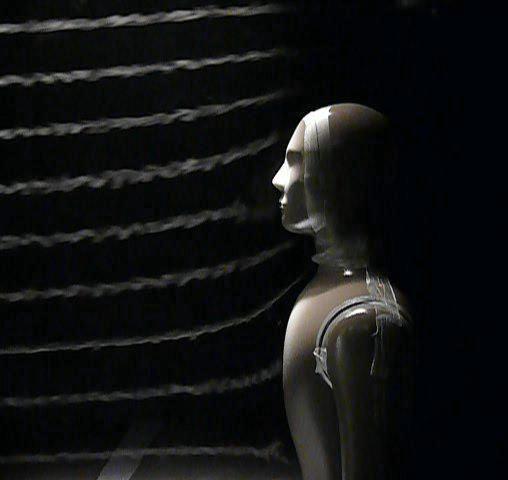
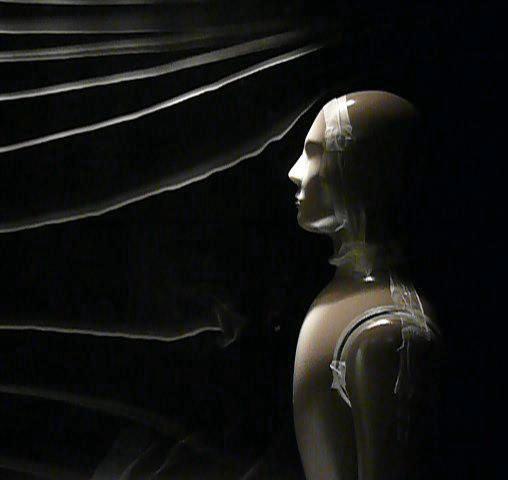
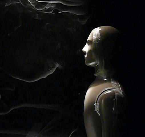
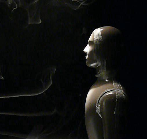
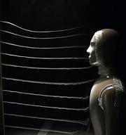
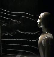
237 Mouth-only 6 L/min 0.42 m/s Unheated Mouth-only 6 L/min 0.42 m/s Heated Mouth-only 20 L/min 0.10 m/s Unheated Mouth-only 20 L/min 0.10 m/s Heated Mouth-only 20 L/min 0.24 m/s Unheated 216

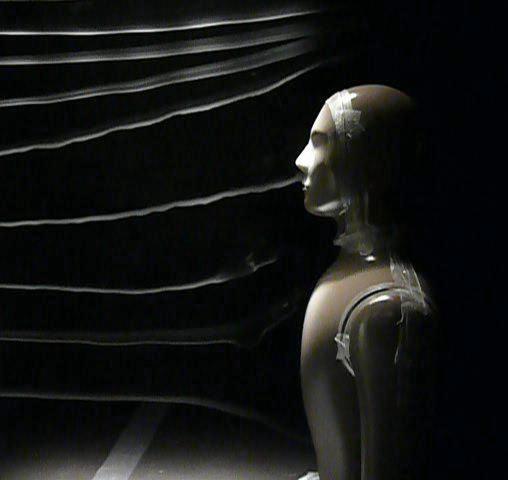
238 Mouth-only 20 L/min 0.24 m/s Heated Mouth-only 20 L/min 0.42 m/s Unheated Mouth-only 20 L/min 0.42 m/s Heated Nose-only 6 L/min 0.10 m/s Unheated Nose-only 6 L/min 0.10 m/s Heated 217

239 Nose-only 6 L/min 0.24 m/s Unheated Nose-only 6 L/min 0.24 m/s Heated Nose-only 6 L/min 0.42 m/s Unheated Nose-only 6 L/min 0.42 m/s Heated Nose-Mouth 6 L/min 0.10 m/s Unheated 218

240 Nose-Mouth 6 L/min 0.10 m/s Heated Nose-Mouth 6 L/min 0.24 m/s Unheated Nose-Mouth 6 L/min 0.24 m/s Heated Nose-Mouth 6 L/min 0.42 m/s Unheated Nose-Mouth 6 L/min 0.42 m/s Heated 219

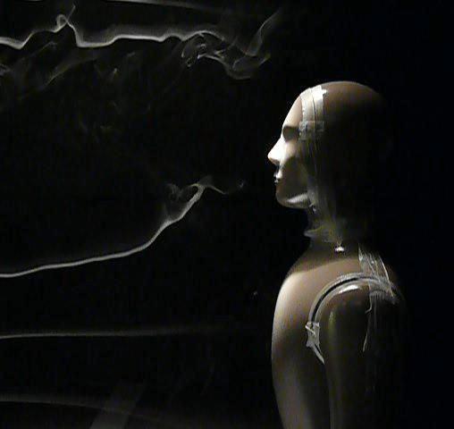
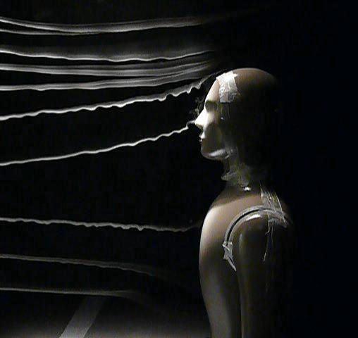
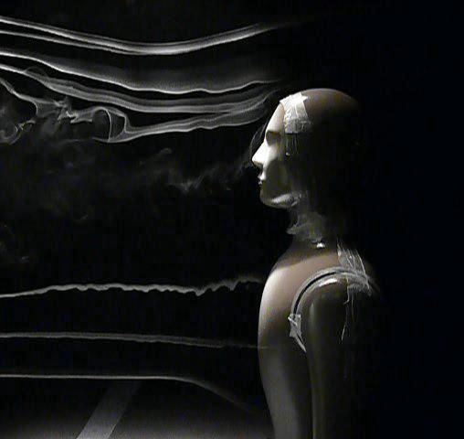
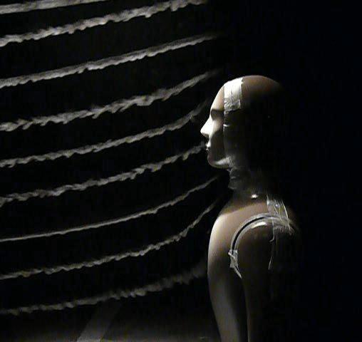
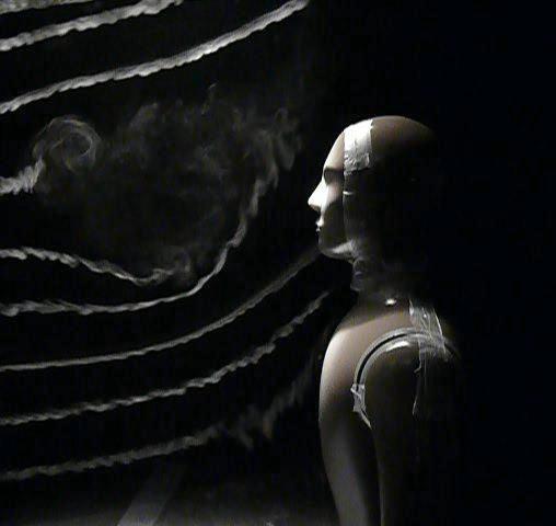
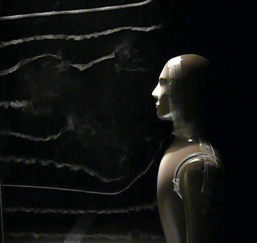
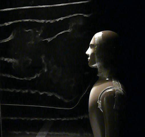
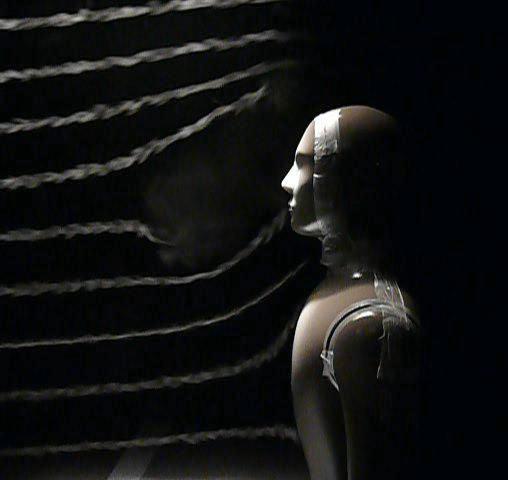
241 Nose-Mouth 20 L/min 0.10 m/s Unheated Nose-Mouth 20 L/min 0.10 m/s Heated Nose-Mouth 20 L/min 0.24 m/s Unheated Nose-Mouth 20 L/min 0.24 m/s Heated Nose-Mouth 20 L/min 0.42 m/s Unheated 220

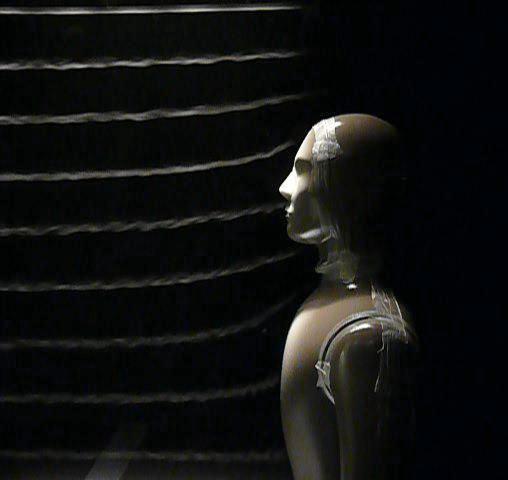
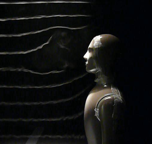
242 Nose-Mouth 20 L/min 0.42 m/s Heated 221

243 Appendix B Complete table of mannequin inhalability data. Highlighted cells indicate experiments performed prior to wind tunnel modification. Powder Grade Mode of Breathing Breathing Flowrate (L/min) Windspeed (m/s) MMAD (µm) σ g Stokes Number F1200 Mouth F1200 Mouth F1200 Mouth F1200 Mouth F1200 Mouth F1200 Mouth F1200 Mouth F1200 Mouth F1200 Mouth F1200 Mouth F1200 Mouth F1200 Mouth F1200 Mouth F1200 Mouth F1200 Mouth F1200 Mouth F1200 Mouth F1200 Mouth F1200 Nose F1200 Nose F1200 Nose F1200 Nose F1200 Nose F1200 Nose F1200 NoseMouth F1200 NoseMouth F1200 NoseMouth F1200 NoseMouth F1200 NoseMouth F1200 NoseMouth F1200 NoseMouth F1200 NoseMouth F1200 NoseMouth F1200 NoseMouth F1200 NoseMouth F1200 NoseMouth F800 Mouth F800 Mouth A 222

244 F800 Mouth F800 Mouth F800 Mouth F800 Mouth F800 Mouth F800 Mouth F800 Mouth F800 Mouth F800 Mouth F800 Mouth F800 Mouth F800 Mouth F800 Mouth F800 Mouth F800 Mouth F800 Mouth F800 Mouth F800 Nose F800 Nose F800 Nose F800 Nose F800 Nose F800 Nose F800 NoseMouth F800 NoseMouth F800 NoseMouth F800 NoseMouth F800 NoseMouth F800 NoseMouth F800 NoseMouth F800 NoseMouth F800 NoseMouth F800 NoseMouth F800 NoseMouth F800 NoseMouth F800 NoseMouth F500 Mouth F500 Mouth F500 Mouth F500 Mouth F500 Mouth F500 Mouth F500 Mouth F500 Mouth F500 Mouth F500 Mouth

245 F500 Mouth F500 Mouth F500 Mouth F500 Mouth F500 Mouth F500 Mouth F500 Mouth F500 Mouth F500 Mouth F500 Mouth F500 Mouth F500 Mouth F500 Mouth F500 Mouth F500 Nose F500 Nose F500 Nose F500 Nose F500 Nose F500 Nose F500 NoseMouth F500 NoseMouth F500 NoseMouth F500 NoseMouth F500 NoseMouth F500 NoseMouth F500 NoseMouth F500 NoseMouth F500 NoseMouth F500 NoseMouth F500 NoseMouth F500 NoseMouth F400 Mouth F400 Mouth F400 Mouth F400 Mouth F400 Mouth F400 Mouth F400 Mouth F400 Mouth F400 Mouth F400 Mouth F400 Mouth F400 Mouth F400 Nose F400 Nose

246 F400 Nose F400 Nose F400 Nose F400 Nose F400 NoseMouth F400 NoseMouth F400 NoseMouth F400 NoseMouth F400 NoseMouth F400 NoseMouth F400 NoseMouth F400 NoseMouth F400 NoseMouth F400 NoseMouth F400 NoseMouth F400 NoseMouth F280 Mouth F280 Mouth F280 Mouth F280 Mouth F280 Mouth F280 Mouth F280 Mouth F280 Mouth F280 Mouth F280 Mouth F280 Mouth F280 Mouth F280 Nose F280 Nose F280 Nose F280 Nose F280 Nose F280 Nose F280 NoseMouth F280 NoseMouth F280 NoseMouth F280 NoseMouth F280 NoseMouth F280 NoseMouth F280 NoseMouth F280 NoseMouth F280 NoseMouth F280 NoseMouth F280 NoseMouth F280 NoseMouth

247 F240 Mouth F240 Mouth F240 Mouth F240 Mouth F240 Mouth F240 Mouth F240 Mouth F240 Mouth F240 Mouth F240 Mouth F240 Mouth F240 Mouth F240 Mouth F240 Mouth F240 Mouth F240 Mouth F240 Nose F240 Nose F240 Nose F240 Nose F240 Nose F240 Nose F240 NoseMouth F240 NoseMouth F240 NoseMouth F240 NoseMouth F240 NoseMouth F240 NoseMouth F240 NoseMouth F240 NoseMouth F240 NoseMouth F240 NoseMouth F240 NoseMouth F240 NoseMouth

248 Appendix C 227

249 228

250 229

251 230

252 231

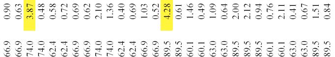
253 232