BUBBLE SIZE, COALESCENCE AND PARTICLE MOTION IN FLOWING FOAMS

Transcription

1 BUBBLE SIZE, COALESCENCE AND PARTICLE MOTION IN FLOWING FOAMS Department of Earth Science and Engineering Imperial College London Kathryn Elizabeth Cole A Thesis Submitted for the Degree of Doctor of Philosophy and Diploma of Imperial College 2010

2 2

3 3

4 Abstract ABSTRACT In minerals processing, froth flotation is used to separate valuable metal minerals from ore. The efficiency of a froth to recover these valuable minerals is closely related to the bubble size distribution through the depth of the froth. Measurement of the bubble size entering the froth and at the froth surface has been achieved previously; however measurement of the bubble size within the froth is extremely difficult as the mineral laden bubble surfaces are opaque and fragile. This work developed a flowing foam column to enable new measurement techniques, in particular visual measurement of the bubble size distribution and velocity profile throughout the depth of the foam. Two phase foam systems share their structure with three phase froth flotation systems, but are transparent in a thin layer. A foam column was constructed to contain a monolayer of overflowing and coalescing foam. This enabled direct measurement of the dynamic bubble size and coalescence through image analysis. The results showed a strong link between column geometry and the foam behaviour. In addition, the measured bubble streamlines closely matched simulated results from a foam velocity model. Positron Emission Particle Tracking (PEPT) is the only existing technique to measure particle behaviour inside froths. In this work, tracer particles with different size and hydrophobicity were tracked in a foam flowing column with PEPT. The particle trajectories were verified with image analysis, thereby increasing confidence in PEPT measurements of opaque flotation systems. The results showed that as hydrophilic tracer particles passed through the foam, their trajectory was determined by the local structure and changes of the foam, such as coalescence events. A hydrophobic tracer particle was involved in drop off and reattachment events, however in the majority of cases still overflowed with the foam. The tracer particle did not always follow the bubble streamlines of the flowing foam, taking instead the shortest path to overflow which cut across streamlines. This work has developed an experimental methodology to validate flowing foam and coalescence models and has developed the necessary techniques to interpret PEPT trajectories in froth flotation.

5 Declaration DECLARATION I declare that no portion of the work referred to in this thesis has been submitted in support of an application for another degree or qualification at this or any other university or institute of learning. Kathryn Cole January 2011

6 Table of Contents TABLE OF CONTENTS ABSTRACT... 4 DECLARATION... 5 LIST OF TABLES... 9 LIST OF FIGURES ACKNOWLEDGMENTS CHAPTER INTRODUCTION Motivation Organisation of the Thesis CHAPTER LITERATURE REVIEW Introduction Minerals Processing Froth Flotation Slurry and the Pulp Phase Froth Overflow Circuits Models of Froth Flotation Models With Coalescence Models of Particle Motion Models of Froth Motion and Cell Design Bubble Size Distribution Measurements Froths Foams Bubble Coalescence Mechanism of Film Rupture Thin Films Binary Coalescence in Liquids Foams Froth Films Particle Motion in Foams and Froths Summary... 42

7 Table of Contents CHAPTER EXPERIMENTAL METHOD WITH FOAM COLUMNS Introduction Flowing Foam Columns Small Overflowing Foam Column (400 mm x 400 mm) Large Overflowing Foam Column (800 mm x 800 mm) Foaming Solution Operation Foam Measurements Image Preparation Proportional Bubble Size Distribution Bubble Area Distribution of the Foaming Space Bubble Velocity Air Recovery Steady State Measurements of Foam Columns Steady State of the Small Overflowing Foam Column Steady State of the Large Overflowing Foam Column Insert Geometries Inserts in the Small Overflowing Foam Column Inserts in the Large Overflowing Foam Column The Effect of Ambient Humidity Summary CHAPTER BUBBLE SIZE, COALESCENCE AND FLOWING PROPERTIES OF OVERFLOWING FOAM Introduction Variation in Air Recovery with Superficial Gas Velocity Variations in The Bubble Speed Distribution and Streamlines with Superficial Gas Velocity Variations in the Bubble Size Distribution with Superficial Gas Velocity Variation in Coalescence with Superficial Gas Velocity Variation in Bubble Area Distribution with Superficial Gas Velocity Geometry Investigation Variation in Air Recovery with Insert Geometry Variations in Bubble Speed Distribution and Streamlines with Insert Geometry Variation in Coalescence with Insert Geometry Variation in Bubble Area Distribution with Insert Geometry Summary

8 Table of Contents CHAPTER POSITRON EMISSION PARTICLE TRACKING IN FLOWING FOAMS Introduction Verification of the PEPT Trajectory with Image Analysis Experimental Method PEPT Trajectory and Foam Profile Time Weighting Function PEPT and Image Correspondence PEPT Tracer Velocity Compared To Local Foam Structure Experimental Method PEPT Trajectory and Foam Velocity Profile PEPT Image Correspondence for an Ascending Tracer PEPT Image Correspondence for a Descending Tracer PEPT in the Large Overflowing Foam Column with Inserts Experimental Method Particle Trajectory in the Large Overflowing Foam Column Particle Trajectories in the Large Overflowing Foam Column with a Small Insert Particle Trajectories in the Large Overflowing Foam Column with a Large Insert Particle Trajectories in the Large Overflowing Foam Column with a Triangular Insert Summary CHAPTER CONCLUSIONS AND FURTHER WORK Conclusions Foam Measurements The Effect of Insert Geometry PEPT Trajectories in Flowing Foam Further work The Effect of Liquid Fraction Statistical Behaviour of Individual Coalescence Events Industrial Crowder Implementation PEPT for Flotation Bubble Size Distribution from a Coalescing Foam Model REFERENCES APPENDICES

9 List of Tables LIST OF TABLES MAIN TEXT Table 3-1: Comparison of the effect of 0.1 g/l xanthan gum on the equilibrium surface tension of two foaming solutions with different concentrations of MIBC Table 3-2: Comparison of values to determine the shear rate dependent viscosity of an aqueous xanthan gum solution at 100 ppm concentration Table 3-3: Values of the minimum, maximum, mean, standard deviation and final value of the unit bubble area for the Triangle 2 insert bubble size distribution measurement Table 3-4: Table showing an example of the data from image analysis (left), converted from pixel units to mm, and the data changed into a two dimensional array with bubble area units in mm Table 4-1: The maximum bubble speed values with superficial gas velocity for experimental and simulated data in the small overflowing foam column Table 4-2: Table showing the different combinations of parent bubbles forming daughters of unit size in binary coalescence, with the number of coalescence events corresponding to each daughter unit size Table 5-1: Different experimental conditions for Tracer 1 including tracer particle properties, PEPT camera and algorithm configuration, and camera recording information Table 5-2: Component errors in the final PEPT image correspondence for Tracer 1 in a rising foam column Table 5-3: Different experimental conditions for Tracer 2 including tracer particle properties, PEPT camera and algorithm configuration, and camera recording information Table 5-4: Component errors in the final PEPT image correspondence for Tracer 2 in a rising foam column APPENDICES Table A 1: Air recovery, average overflowing velocity and overflowing froth depth in the small overflowing foam column at different superficial gas velocities Table A 2: Horizontal foam velocity (mm/s) relative to the bottom-left of the column at different grid positions (mm) in the small overflowing foam column at a superficial gas velocity of 5.2 cm/s Table A 3: Vertical foam velocity (mm/s) relative to the bottom-left of the column at different grid positions (mm) in the small overflowing foam column at a superficial gas velocity of 5.2 cm/s Table A 4: Horizontal foam velocity (mm/s) relative to the bottom-left of the column at different grid positions (mm) in the small overflowing foam column at a superficial gas velocity of 8.3 cm/s Table A 5: Vertical foam velocity (mm/s) relative to the bottom-left of the column at different grid positions (mm) in the small overflowing foam column at a superficial gas velocity of 8.3 cm/s

10 List of Tables Table A 6: Horizontal foam velocity (mm/s) relative to the bottom-left of the column at different grid positions (mm) in the small overflowing foam column at a superficial gas velocity of 12.5 cm/s Table A 7: Vertical foam velocity (mm/s) relative to the bottom-left of the column at different grid positions (mm) in the small overflowing foam column at a superficial gas velocity of 12.5 cm/s Table A 8: Horizontal foam velocity (mm/s) relative to the bottom-left of the column at different grid positions (mm) in the small overflowing foam column at a superficial gas velocity of 14.6 cm/s Table A 9: Vertical foam velocity (mm/s) relative to the bottom-left of the column at different grid positions (mm) in the small overflowing foam column at a superficial gas velocity of 14.6 cm/s Table A 10: Horizontal foam velocity (mm/s) relative to the bottom-left of the column at different grid positions (mm) in the small overflowing foam column at a superficial gas velocity of 15.6 cm/s Table A 11: Vertical foam velocity (mm/s) relative to the bottom-left of the column at different grid positions (mm) in the small overflowing foam column at a superficial gas velocity of 15.6 cm/s Table A 12: Proportions of bubbles of different unit size and total number of bubbles counted per measurement in the lower half of the small overflowing foam column for different superficial gas velocities Table A 13: Proportions of bubbles of different unit size and total number of bubbles counted per measurement in the upper half of the small overflowing foam column for different superficial gas velocities Table A 14: Proportions of bubbles of different unit size and total number of bubbles counted per measurement in the total small overflowing foam column for different superficial gas velocities Table A 15: The average bubble area (mm 2 ) at different grid positions (mm) in the small overflowing foam column at a superficial gas velocity of 5.2 cm/s Table A 16: The average bubble area (mm 2 ) at different grid positions (mm) in the small overflowing foam column at a superficial gas velocity of 8.3 cm/s Table A 17: The average bubble area (mm 2 ) at different grid positions (mm) in the small overflowing foam column at a superficial gas velocity of 12.5 cm/s Table A 18: The average bubble area (mm 2 ) at different grid positions (mm) in the small overflowing foam column at a superficial gas velocity of 14.6 cm/s Table A 19: The average bubble area (mm 2 ) at different grid positions (mm) in the small overflowing foam column at a superficial gas velocity of 15.6 cm/s Table A 20: The mean air recovery, standard deviation in air recovery, wetting perimeter and cross sectional area of a range of different inserts in the small overflowing foam column at a superficial gas velocity of 5.2 cm/s Table A 21: Horizontal foam velocity (mm/s) relative to the bottom-left of the column at different grid positions (mm) in the small overflowing foam column with the 2 cm x 12.5 cm insert at a superficial gas velocity of 5.2 cm/s Table A 22: Vertical foam velocity (mm/s) relative to the bottom-left of the column at different grid positions (mm) in the small overflowing foam column with the 2 cm x 12.5 cm insert at a superficial gas velocity of 5.2 cm/s Table A 23: Horizontal foam velocity (mm/s) relative to the bottom-left of the column at different grid positions (mm) in the small overflowing foam column with the 5 cm x 5 cm insert at a superficial gas velocity of 8.3 cm/s

11 List of Tables Table A 24: Vertical foam velocity (mm/s) relative to the bottom-left of the column at different grid positions (mm) in the small overflowing foam column with the 5 cm x 5 cm insert at a superficial gas velocity of 8.3 cm/s Table A 25: Horizontal foam velocity (mm/s) relative to the bottom-left of the column at different grid positions (mm) in the small overflowing foam column with the 8 cm x 3.1 cm insert at a superficial gas velocity of 12.5 cm/s Table A 26: Vertical foam velocity (mm/s) relative to the bottom-left of the column at different grid positions (mm) in the small overflowing foam column with the 8 cm x 3.1 cm insert at a superficial gas velocity of 12.5 cm/s Table A 27: Horizontal foam velocity (mm/s) relative to the bottom-left of the column at different grid positions (mm) in the small overflowing foam column with the 8 cm x 12.5 cm insert at superficial gas velocity 14.6 cm/s Table A 28: Vertical foam velocity (mm/s) relative to the bottom-left of the column at different grid positions (mm) in the small overflowing foam column with the 8 cm x 12.5 cm insert at superficial gas velocity 14.6 cm/s Table A 29: Horizontal foam velocity (mm/s) relative to the bottom-left of the column at different grid positions (mm) in the small overflowing foam column with the Triangle 2 insert at a superficial gas velocity of 15.6 cm/s Table A 30: Vertical foam velocity (mm/s) relative to the bottom-left of the column at different grid positions (mm) in the small overflowing foam column with the Triangle 2 insert at a superficial gas velocity of 15.6 cm/s Table A 31: Proportions of bubbles of different unit size and total number of bubbles counted per measurement in the lower half, upper half and over the total area of the small overflowing foam column with different inserts at a superficial gas velocity of 5.2 cm/s Table A 32: The average bubble area (mm 2 ) at different grid positions (mm) in the small overflowing foam column with the 2 cm x 12.5 cm insert at a superficial gas velocity of 5.2 cm/s Table A 33: The average bubble area (mm 2 ) at different grid positions (mm) in the small overflowing foam column with the 5 cm x 5 cm insert at a superficial gas velocity of 5.2 cm/s Table A 34: The average bubble area (mm 2 ) at different grid positions (mm) in the small overflowing foam column with the 8 cm x 3.1 cm insert at a superficial gas velocity of 5.2 cm/s Table A 35: The average bubble area (mm 2 ) at different grid positions (mm) in the small overflowing foam column with the 8 cm x 12.5 cm insert at a superficial gas velocity of 5.2 cm/s Table A 36: The average bubble area (mm 2 ) at different grid positions (mm) in the small overflowing foam column with the Triangle 2 insert at a superficial gas velocity of 5.2 cm/s Table B 1: Different coalescence events occurring during 0.405s in the small foam column at steady state and a superficial gas velocity of 5.2 cm/s

12 List of Figures LIST OF FIGURES MAIN TEXT Figure 2-1: Flow chart with photographs of the stages of minerals processing to obtain the finished product from ore Figure 2-2: Schematic of a flotation tank Figure 2-3: Schematic of different bubble structures in the pulp and the froth with attached (black) and entrained (grey) particles (Hatfield, 2006: p.34) Figure 2-4: Variation in air recovery with air flowrate (left) (Barbian et al., 2006: p. 4) and the effect of aeration on flotation bank performance (right) (Hadler & Cilliers, 2009: p. 4) Figure 2-5: Photographs of different launder and crowder designs on industrial flotation cells, with the froth flow direction shown as arrows. A Linear launders with a triangular cross section on a cylindrical flotation column; B Linear launders on a rectangular flotation tank; C Crowder on a flotation tank, directing froth to overflow the weir Figure 2-6: Images of flotation tanks in banks and circuits Figure 2-7: Graphs showing the entrainment factor as a function of particle size (Neethling & Cilliers, 2009: p. 5, including experimental relationships from Savassi et al. (1998) and Zheng et al. (2006)) Figure 2-8: Froth motion model of a cylindrical industrial flotation cell (Zheng et al., 2004: p. 4) Figure 2-9: Froth crowder and concentrate launder configuration from an industrial flotation cell (Zheng & Knopjes, 2004: p. 3) Figure 2-10: Photographs of bubbles from the pulp (left) and films at the froth surface (right) Figure 2-11: Photographs of a foam showing the changes in bubble size and shape with height (left) and an aqueous foam showing key features (right) Figure 2-12: Typical bubble break up sequence recorded at 100 frames per second (Caps et al., 2006: p. 3) Figure 2-13: Diagram showing the bridging effect of particles on films, where the contact angle θ is shown for A, a hydrophilic particle and B, a strongly hydrophobic particle (Aveyard et al., 1994: p. 7) Figure 2-14: Trajectory of a galena tracer particle as it moves through the froth and over the weir in different planes and views (Waters et al., 2008b: p. 4) Figure 3-1: Schematic of the small foam column, with measurements in millimetres. The plate separation is 5 mm. 45 Figure 3-2: Photograph of the small overflowing foam column Figure 3-3: Schematic of the large foam column with measurements in millimetres. The plate separation is 5 mm Figure 3-4: Photograph of the large foam column... 48

13 List of Figures Figure 3-5: Graphs showing the viscosity with shear rate for a dilute (0.1 g/l) xanthan gum solution. Results from Whitcomb & Macosko (1978) are shown on the left, and the results from this work on the right Figure 3-6: Experimental set-up in plan view Figure 3-7: Image processing used to segregate the Plateau border network and gas cells from an image of the foam profile Figure 3-8: Example of extracting a sample for measuring the unit bubble size from the lower half of each image Figure 3-9: Histogram of the bubble area (left) and the proportion of bubbles of unit size (right) for a superficial gas velocity of 5.2 cm/s Figure 3-10: Sample bubble image and quiver plot combined to show the bubble velocity in pixels between two consecutive frames Figure 3-11: Graph showing the average height with time of the small overflowing column at a superficial gas velocity of 5.2 cm/s. The top of the column is shown as a dashed line Figure 3-12: Graph showing the change in air recovery with time for the small overflowing column at a superficial gas velocity of 5.2 cm/s Figure 3-13: Graph showing the variation in the unit bubble size with time Figure 3-14: Graph showing the proportion of bubbles of different sizes with time for the small overflowing column at a superficial gas velocity of 5.2 cm/s Figure 3-15: Graph showing the variation in the overflowing foam height in the large overflowing foam column with time, at a superficial gas velocity of 5.7 cm/s Figure 3-16: Graph showing the fluctuation in the overflowing foam height in the large column during a period of 3 seconds at a superficial gas velocity of 5.7 cm/s Figure 3-17: Diagrams showing the different depths (mm) used with 2cm, 5cm and 8cm wide inserts in the foaming space of the small overflowing foam column Figure 3-18: Diagrams showing the dimensions (mm) of triangular inserts in the foaming space of the small overflowing foam column Figure 3-19: Images of the small overflowing foam column with a rectangular insert of 2 cm width at various depths (cm) at a superficial gas velocity of 5.2 cm/s Figure 3-20: Images of the small overflowing foam column with a rectangular insert of 5 cm width at various depths (cm) at a superficial gas velocity of 5.2 cm/s Figure 3-21: Images of the small overflowing foam column with a rectangular insert of 8 cm width at various depths (cm) at a superficial gas velocity of 5.2 cm/s Figure 3-22: Images of the small overflowing foam column with different shaped inserts at a superficial gas velocity of 5.2 cm/s

14 List of Figures Figure 3-23: Diagrams showing the dimensions of different inserts used in the foaming space of the large overflowing foam column, with measurements in mm. The inserts were positioned at depths relative to the mid- point of the column Figure 3-24: Photographs of the large overflowing column with different inserts at a superficial gas velocity of 5.7 cm/s Figure 3-25: Graph showing the effect of ambient humidity on air recovery of the small overflowing foam column with 8x3.1 insert at a superficial gas velocity of 5.2 cm/s Figure 4-1: Images of the small overflowing column at different superficial gas velocities, 5.2 to 10.4 cm/s Figure 4-2: Images of the overflowing small column at different superficial gas velocities, 11.5 to 15.6 cm/s Figure 4-3: Graph showing the change in air recovery with superficial gas velocity for the small overflowing foam column Figure 4-4: Graph showing the variation of foam depth overflowing the weir with superficial gas velocity for the small overflowing foam column Figure 4-5: Graph showing the variation of the average overflowing bubble velocity with superficial gas velocity for the small overflowing foam column Figure 4-6: Plot showing the experimental flow streamlines and average speed distribution in mm/s (left), and plot showing the simulated flow streamlines and foam velocity distribution in m/s (right), for the overflowing small column at a superficial gas velocity of 5.2 cm/s Figure 4-7: Plot showing the experimental flow streamlines and average speed distribution in mm/s (left), and plot showing the simulated flow streamlines and foam velocity distribution in m/s (right), for the overflowing small column at a superficial gas velocity of 8.3 cm/s Figure 4-8: Plot showing the experimental flow streamlines and average speed distribution in mm/s (left), and plot showing the simulated flow streamlines and foam velocity distribution in m/s (right), for the overflowing small column at a superficial gas velocity of 12.5 cm/s Figure 4-9: Plot showing the experimental flow streamlines and average speed distribution in mm/s (left), and plot showing the simulated flow streamlines and foam velocity distribution in m/s (right), for the overflowing small column at a superficial gas velocity of 14.6 cm/s Figure 4-10: Plot showing the experimental flow streamlines and average speed distribution in mm/s (left), and plot showing the simulated flow streamlines and foam velocity distribution in m/s (right), for the overflowing small column at a superficial gas velocity of 15.6 cm/s Figure 4-11: Graph showing the numbers of bubbles counted in the small overflowing foam column operated at different superficial gas velocities Figure 4-12: Chart showing the proportion of bubbles of different unit size in the lower half of the small overflowing column operated at different superficial gas velocities Figure 4-13: Chart showing the proportion of bubbles of different unit size in the upper half of the small overflowing column operated at different superficial gas velocities

15 List of Figures Figure 4-14: Chart showing the proportion of bubbles of different unit size for the total area of the small overflowing column operated at different superficial gas velocities Figure 4-15: Average bubble size distribution (in mm 2 ) and flow streamlines for the overflowing small column at different superficial gas velocities (cm/s) Figure 4-16: Graph showing the variation in air recovery with insert width for different insert widths in the small overflowing foam column at a superficial gas velocity of 5.2 cm/s Figure 4-17: Graph showing the variation in air recovery with insert depth for different insert widths in the small overflowing foam column at a superficial gas velocity of 5.2 cm/s Figure 4-18: Graph showing the variation in air recovery with insert wetted perimeter with lines of constant depth, for a range of inserts in the small overflowing foam column at a superficial gas velocity of 5.2 cm/s Figure 4-19: Graph showing the variation in air recovery with insert area with lines of constant depth, for a range inserts in the small overflowing foam column at a superficial gas velocity of 5.2 cm/s Figure 4-20: Plot showing the experimental (left, mm/s) and simulated (right, m/s) flow streamlines and average bubble speed distribution with the 2x12.5 insert in the small overflowing foam column at a superficial gas velocity of 5.2 cm/s Figure 4-21: Plot showing the experimental (left, mm/s) and simulated (right, m/s ) flow streamlines and average bubble speed distribution with the 5x5 insert in the small overflowing foam column at a superficial gas velocity of 5.2 cm/s Figure 4-22: Plot showing the experimental (left, mm/s) and simulated (right, m/s) flow streamlines and average bubble speed distribution with the 8x3.1 insert in the small overflowing foam column at a superficial gas velocity of 5.2 cm/s Figure 4-23: Plot showing the experimental (left, mm/s) and simulated (right, m/s) flow streamlines and average bubble speed distribution with the 8x3.1 insert in the small overflowing foam column at a superficial gas velocity of 5.2 cm/s Figure 4-24: Plot showing the experimental (left, mm/s) and simulated (right, m/s) flow streamlines and average bubble speed distribution with the Triangle 2 insert in the small overflowing foam column at a superficial gas velocity of 5.2 cm/s Figure 4-25: Graph showing the variation in the area of the unit bubble measured in the small overflowing foam column with different inserts Figure 4-26: Graph showing the total number of bubbles counted in the small overflowing foam column at a superficial gas velocity of 5.2 cm/s for a number of rectangular inserts with depth Figure 4-27: Charts showing the proportion of bubbles of different unit size in the lower half of the small overflowing foam column at a superficial gas velocity of 5.2 cm/s with different inserts Figure 4-28: Charts showing the proportion of bubbles of different unit size in the upper half of the small overflowing foam column at a superficial gas velocity of 5.2 cm/s with different inserts Figure 4-29: Charts showing the proportion of bubbles of different unit size for the total area of the small overflowing foam column at a superficial gas velocity of 5.2 cm/s with different inserts

16 List of Figures Figure 4-30: Average bubble area distribution (in mm 2 ) and flow streamlines in the small overflowing foam column at a superficial gas velocity of 5.2 cm/s with a 2x12.5 cm insert Figure 4-31: Average bubble area distribution (in mm 2 ) and flow streamlines in the small overflowing foam column at a superficial gas velocity of 5.2 cm/s with a 5x5 cm insert Figure 4-32: Average bubble area distribution (in mm 2 ) and flow streamlines in the small overflowing foam column at a superficial gas velocity of 5.2 cm/s with a 8x3.1 cm insert Figure 4-33: Average bubble area distribution (in mm 2 ) and flow streamlines in the small overflowing foam column at a superficial gas velocity of 5.2 cm/s with a 8x12.5 cm insert Figure 4-34: Average bubble area distribution (in mm 2 ) and flow streamlines in the small overflowing foam column at a superficial gas velocity of 5.2 cm/s with the Triangle 2 insert Figure 5-1: Schematic diagram of the non-overflowing foam column (left), with measurements in mm, and a photograph of the rising foam (right) Figure 5-2: Diagram showing the position of the foam column within the PEPT camera (left) and a photograph of the experimental set up (right). The foam column contains black dye not used in these experiments Figure 5-3: Graph showing the tracer descent during 14.3 seconds within the column (dashed line) Figure 5-4: Optical image analysis measurement of the vertical foam velocity profile near the bottom of the column, across its width for a superficial gas velocity of 2.7 cm/s Figure 5-5: Graph showing the kernel for a time weighting function composed of cubic splines for interpolating and smoothing the PEPT trajectory Figure 5-6: Graphs of the tracer trajectory with time measured with PEPT, with the vertical (y) direction with time during 2 seconds above and the horizontal (z) direction with time during 2 seconds below. The unprocessed data is shown on the left, and the trajectory smoothed with time weighting kernel width 200 ms is on the right Figure 5-7: A sequence of digital images with final PEPT correspondence co-ordinates shown as a white circle with radius corresponding to total error. The points were produced with a time weighting function kernel width of 200 ms. The tracer image location is visible as a black spot. Each image size corresponds to 5 cm x 5 cm with a scale of 1 pixel/mm Figure 5-8: Optical image analysis measurement of the foam vertical velocity profile at the top of the column, across its width at a superficial gas velocity of 4.4 cm/s Figure 5-9: Total trajectory of the 70 μm tracer in the foam column during 10 seconds; the unprocessed PEPT data is on the left, and the trajectory smoothed with time weighting kernel width 200 ms is on the right. The tracer starts at the base in the centre, moves up and then down the left side of the column Figure 5-10: Focus section of the 70 μm tracer ascent in the foam column; the unprocessed PEPT data is on the left, and the trajectory smoothed with time weighting kernel width 200 ms is on the right. The tracer starts at the bottom right and moves upwards Figure 5-11: Graph showing the vertical velocity of Tracer 2 (70 μm diameter) with time for a focus section of the tracer ascent measured with PEPT and processed with time weighting kernel width 200 ms

17 List of Figures Figure 5-12: Image sequence corresponding to the tracer descent shown in Figure 5-11, where times shown are in seconds. The tracer path, measured with PEPT and processed with time weighting with kernel width 200 ms, is shown as a dot with diameter corresponding to the total error. Each image size corresponds to 3.6 cm x 2.5 cm with a scale of 6 pixels/mm Figure 5-13: Focus section of the 70 μm tracer descent in the foam column; the unprocessed PEPT data is on the left, and the trajectory smoothed with time weighting kernel width 200 ms is on the right. The tracer starts at the top and moves downwards Figure 5-14: Graph showing the vertical velocity of Tracer 2 (70 μm diameter) with time for a focus section of the tracer descent measured with PEPT and processed with time weighting kernel width 200 ms Figure 5-15: Image sequence corresponding to the tracer descent shown in Figure 5-14, where the time intervals are in seconds. The tracer path, measured with PEPT and processed with time weighting with a kernel width of 200 ms, is shown as a white dot with diameter equalling the total error. Each image corresponds to the size 5.7 cm x 2.1 cm with a scale of 6 pixels/mm Figure 5-16: Photograph showing the experimental set up for the investigation into the insert effect on particle motion in the large overflowing foam column. The foam column contains pink dye not used in any of the experiments Figure 5-17: Scanning Electron Microscope images of the tracer particle with a hydrophobic coating at 100 and 500 times magnification Figure 5-18: Graph showing three hydrophobic particle trajectories that overflowed the weir at different times in the large overflowing foam column at a superficial gas velocity of 4.3 cm/s Figure 5-19: Graph showing three hydrophobic particle trajectories that overflowed the weir at different times in the large overflowing foam column at a superficial gas velocity of 4.3 cm/s Figure 5-20: Graph showing five hydrophobic particle trajectories that overflowed the weir at different times in the large overflowing foam column at a superficial gas velocity of 4.3 cm/s Figure 5-21: Graph showing four hydrophobic particle trajectories that overflowed the weir at different times in the large overflowing foam column with the small insert at a superficial gas velocity of 4.3 cm/s Figure 5-22: Graph showing six hydrophobic particle trajectories that overflowed the weir after particle drop off at different times in the large overflowing foam column with the small insert at a superficial gas velocity of 4.3 cm/s. 135 Figure 5-23: Graph showing three hydrophobic particle trajectories that did not overflow the weir at different times in the large overflowing foam column with the small insert at a superficial gas velocity of 4.3 cm/s Figure 5-24 : Graph showing two hydrophobic particle trajectories that overflowed the weir at different times in the large overflowing foam column with the large insert at a superficial gas velocity of 4.3 cm/s Figure 5-25: Graph showing five hydrophobic particle trajectories that overflowed the weir after particle drop off at different times in the large overflowing foam column with the large insert at a superficial gas velocity of 4.3 cm/s. 137 Figure 5-26: Graph showing five hydrophobic particle trajectories that overflowed the weir after particle drop off at different times in the large overflowing foam column with the large insert at a superficial gas velocity of 4.3 cm/s

18 List of Figures Figure 5-27: Graph showing two hydrophobic particle trajectories that did not overflow the weir at different times in the large overflowing foam column with the large insert at a superficial gas velocity of 4.3 cm/s Figure 5-28: Graph showing three hydrophobic particle trajectories that did not overflow the weir at different times in the large overflowing foam column with the large insert at a superficial gas velocity of 4.3 cm/s Figure 5-29: Graph showing two hydrophobic particle trajectories that overflowed the weir at different times in the large overflowing foam column with the triangle insert at a superficial gas velocity of 4.3 cm/s Figure 5-30: Graph showing two hydrophobic particle trajectories that overflowed the weir after particle drop off at different times in the large overflowing foam column with the triangle insert at a superficial gas velocity of 4.3 cm/s Figure 5-31: Graph showing three hydrophobic particle trajectories that did not overflow the weir at different times in the large overflowing foam column with the triangle insert at a superficial gas velocity of 4.3 cm/s Figure 6-1: Graphs showing the experimental and simulation bubble size distributions for different heights in a nonoverflowing foam APPENDICES Figure B 1: Graph showing the proportion of different coalesced bubble sizes for a sample during 0.405s Figure B 2: Graph showing the frequency of parent bubbles of different size coalescing with bubbles of size unit 1, for a sample during 0.405s Figure B 3: Chart showing the location of different coalescence types according to unit daughter bubble size within the small foam column at a superficial gas velocity of 5.2 cm/s Figure B 4: Graph showing the frequency of different angles between the centre of bubbles involved in coalescence in the small overflowing column at a superficial gas velocity of 5.2 cm/s

19 Acknowledgments ACKNOWLEDGMENTS In no particular order, my thanks to: My PhD supervisor, Prof Jan Cilliers, for his guidance and encouragement throughout this work; Dr. Stephen Neethling for answering many questions and helping with code; Dr. Kathryn Hadler for her unswerving support; Dr. Pablo Brito-Parada and Dr. Mingming Tong for going out of their way to help me with simulations; Dr. Mark Pursell, Dr. Chris Smith, Dr. Gareth Morris, Barry Shean and the rest of the Froth and Foam Research Group for their assistance during experiments and being useful sounding boards; Christine Xu and Ryan Cunningham for their help in writing image processing algorithms; Graham Nash, Alex Toth and the guys at the Chemical Engineering workshop for their expertise in making experimental rigs; The team at the University of Birmingham with support from Dr. Kriss Waters without whom I would not have been able to complete PEPT experiments; EPSRC for funding this PhD, and Teachers Pensions so that I could afford to live a little; The C R Barber Trust at the Institute of Physics and the International Travel Grant at the Royal Academy of Engineering to allow me to attend an international conference; Greg Wilson and his amazing mixes for late night writing sessions; My grandparents, Jim and Doris, for their strength; My mum, Liz, and sisters, Anna and Jenny, for always being there, especially when it s difficult; Ollie, for being there every day and supporting me when I had to give a little extra; Two dads - Nigel for inspiring me to do a PhD, and my own who never knew I would end up doing a PhD but believed in me. I wish I could share this with you both.

20 Chapter 1: Introduction CHAPTER 1 INTRODUCTION 1.1 MOTIVATION Global demand for metal minerals is increasing. Meeting this demand is not straightforward as securing new resources has become increasingly politically complex and new mines are expensive due to large capital costs in construction. Modern attitudes towards the environment have changed, and mining companies must show that they can behave in a responsible and sustainable way. One of the processes required to obtain metal minerals from ore is froth flotation. This is a mineral separation process that differentiates between fine ( μm) mineral particles based on their hydrophobicities in a flowing froth. More than 3 billion tons of ore is treated by flotation annually to recover the valuable metal minerals. Despite this high tonnage, flotation is still ill-understood and remarkably inefficient as much as 10% of the recoverable mineral may be discarded. Enhancing flotation efficiency via technology or productivity will make the supply of new minerals more sustainable. Two decades of research into physical models of foam drainage and solids motion within froths has lead to the development of Computational Fluid Dynamics, CFD, models of froth flotation. A significant aspect of the froth behaviour is the effect of coalescence. Excessive amounts of coalescence decrease the area of bubble surface available for solids loading. The bubble size entering the froth has already been measured (Chen et al., 2001), and the bubble size at the froth surface is used to control flotation efficiency (Yang et al., 2009). However recent studies have highlighted the fact that the surface bubble size distribution may not be representative of the froth interior (Wang & Neethling, 2006). Measurement of the bubble size within the froth is difficult as the froth is opaque and fragile. The first aim of this project is to develop an overflowing foam column, where the bubble size distribution can be measured optically over the entire height of the column. Previously, the bubble size distribution in

21 Chapter 1: Introduction foam has been inadequately measured with techniques such as electrical resistance (Xie et al. 2004) where the technique was limited by the system resolution, or X-ray tomography (Lambert et al., 2005) which requires a stable foam due to lengthy processing times. Optical bubble size measurements through a container wall are not a true representation of the internal bubble size distribution (Cheng & Lemlich, 1983). In this work, a Hele-Shaw column was designed and constructed to study the behaviour of a monolayer of bubbles, or quasi 2D foam. Hele-Shaw columns are typically non-overflowing (eg. Cox & Janiaud, 2008; Caps et al., 2006). This is the first time that the properties of an overflowing 2D foam in a vertical Hele-Shaw column have been investigated. A chemical system was designed to provide a dynamic, coalescing foam that overflowed and burst at the foam surface. High speed images and videos of the foam were captured to enable measurement of the properties of individual bubbles in the 2D foam column. Therefore the evolving bubble size distribution can be related to the bubble velocity and average flow streamlines. The overflowing foam behaviour was quantified in terms of the air recovery, or amount of air that overflows as unburst bubbles. Recent studies have highlighted a link between the air recovery and performance of a flotation cell (Ventura Medina et al., 2003; Barbian et al., 2006). Therefore the inclusion of air recovery in this analysis allows direct comparison to a flotation cell. The recent trend in flotation technology has been to increase the size of the flotation cell, which increases the froth volume. To increase the recovery, crowders and launders have been placed in the froth zone to increase the volume of overflowing froth. However, this has not been done with adequate knowledge of the effect on the froth behaviour. The second aim of this project is to investigate the effects of different inserts on the overflowing foam behaviour. If there is an optimum crowder geometry that will maximise flotation performance, this has huge potential benefits for the mining industry. The application of Positron Emission Particle Tracking, or PEPT, to froth flotation was pioneered at Imperial College London to investigate bubble-particle behaviour (Waters et al., 2008a; Waters et al., 2008b). However, the initial results revealed complicated particle behaviour within the froth that could not be adequately explained. In this project, the trajectories of hydrophilic particles were measured with PEPT in a rising foam column and combined with image analysis of the foam structure. The changes in particle trajectory could be explained by foam structure and events, such as coalescence. Then hydrophobic particles were tracked in an overflowing foam column to relate particle attachment and detachment to the evolving bubble size and speed distribution with column geometry. The achievement of these goals will provide a new understanding of processes within the froth, such as coalescence. By combining multi modal measurements of image analysis and PEPT, the effect of insert geometry on the flowing foam behaviour can be ascertained. Furthermore, the complex particle trajectories measured in flotation froths with PEPT can be fully explained with the techniques developed in this work. These components can be included in the next generation of CFD flotation models, to increase flotation efficiency through system optimisation or improvements in equipment design. 1.2 ORGANISATION OF THE THESIS The thesis is organised according to the outline given above. Chapter 2 is a review of previously published work. The role of froth flotation in minerals processing is explained, followed by a description of the main 21

22 Chapter 1: Introduction parts of a typical flotation cell and how they enable particle separation. The provision for coalescence and particle motion in models of flotation is presented, with the current state of the art for measurements of coalescence and the bubble size distribution within froths and foams. Chapter 3 is a description of the two overflowing foam columns developed in this work: one small (400 mm x 400 mm) for bubble size measurements and one large (800 mm x 800 mm) to track particles with PEPT. The properties of a foaming solution developed to produce a coalescing foam are explained, along with the time required for the foam to achieve steady state and its duration. Different foam measurements performed with image analysis are described: the methods for measuring the bubble size distribution, the bubble speed distribution, average bubble tracks and air recovery. The geometries of the different inserts are also included in this chapter. Chapter 4 presents the results of image analysis measurements from the small overflowing foam column with different superficial gas velocities and insert geometries. The bubble speed distribution and bubble tracks from experiment are compared to simulations of the streamlines over the foaming space. The bubble size distribution is analysed in detail, in terms of the proportions of bubbles of different sizes and their distribution over the foaming space. The optimum insert geometry is determined for the air recovery and bubble size distribution. In Chapter 5, the results of tracking different tracer particles with PEPT are discussed. A large tracer was tracked with PEPT and image analysis, to test the accuracy of the PEPT trajectory. This enables the combination of PEPT trajectories and image analysis to explain changes in the PEPT trajectory of a smaller tracer particle that is too small to be observed visually. The behaviour displayed by a hydrophobic particle in the large overflowing foam column with different inserts is discussed, and compared to the streamlines measured in the small overflowing column. Chapter 6 is the final chapter in this work, and presents conclusions and future work that could be undertaken to develop an empirical model of coalescence in overflowing 2D foams, and to interpret PEPT trajectories measured in flotation froths. The appendix presents multiple journal publications developed during this course of study. Three have been peer-reviewed and published online, and the final paper has been submitted for peer review. 22

23 Chapter 2: Literature Review CHAPTER 2 LITERATURE REVIEW 2.1 INTRODUCTION This chapter will introduce minerals processing, the series of industrial processes that are used to transform ore to mineral concentrates in a useable form. Froth flotation is a key stage, where the valuable metal mineral grains are separated from any waste particles. Froth flotation will be described in detail, including the design of the equipment and how the structure of a froth determines the particle separation process. The air recovery, or amount of unburst bubbles that overflow to the concentrate, will be presented as an important indicator of flotation performance. Recent simulations of froth flotation include models for coalescence, the dispersion of liquid and particles within the froth, and how cell design affects the motion of the froth. Major contributions to each of these areas of modelling will be described in this chapter. Foams share froth structure, but do not contain the solid phase. The difficulties in measuring the bubble size distribution in foams will be discussed, despite the optical transparency of individual films. Next, the process of bubble coalescence will be described, including what it is, what causes film rupture and how it has been measured in liquids. Experiments and models highlighting the role of the size and shape of containers on foam and froth behaviour will also be included. Positron Emission Particle Tracking (PEPT) uses penetrating radiation and can therefore track particles inside opaque multi phase systems. The technique will be described, along with some issues to be countered in order to measure particle behaviour inside flotation froths.

24 Chapter 2: Literature Review 2.2 MINERALS PROCESSING Metal production underpins the industrialised world that we know today. For example, copper is used in many applications, such as power, housing and transport. An important source of copper is sulphide minerals, which are present as small grains of valuable mineral within a larger mass of undesirable material. Initially, the ore is mined and then the minerals must be liberated by a series of crushing, grinding and milling processes, as shown in Figure 2-1. The next stage involves separating the valuable minerals grains from the waste. Separation exploits differences in particle properties, such as specific gravity or magnetism (Wills, 2006). Flotation is the most common separation process, and employs the difference in surface properties of valuable minerals and waste, or gangue, material to separate them (Wills, 2006). There is an optimum size for flotation to ensure the particle adheres to the bubble and therefore overflows to the concentrate rather than being lost as tailings. Jameson et al. (2007) cite a range of 10 to 70 μm for successful flotation of base metal minerals, however the particle density ultimately determines the optimum size range for each mineral species. Outside of this range, recovery decreases with ultrafine and coarse particles. After flotation, the valuable mineral concentrate can then be removed for further processing such as smelting. Figure 2-1: Flow chart with photographs of the stages of minerals processing to obtain the finished product from ore. 2.3 FROTH FLOTATION A typical flotation cell is shown in Figure 2-2. Slurry is pumped into the base of the cell, where it is agitated by an impeller and aerated. The valuable mineral particles attach to bubbles in the pulp phase of the cell, and rise to the surface. The bubbles begin to pack to form the froth phase of the column. The froth concentrate overflows the cell walls, for further processing such as smelting. In practice some gangue 24

25 Chapter 2: Literature Review becomes entrained in the froth, which reduces the grade of the concentrate. Grade is a key indicator of flotation efficiency, and is a measure of the quality of the final product. Recovery is defined as the percentage of total valuable mineral that reaches the concentrate stream compared to the amount present in the ore (Wills, 2006). This section will describe the different components of a flotation cell: the slurry, the pulp phase, the froth phase and the overflow, along with a description of how flotation cells are arranged. Froth Concentrate Overflow Tailings Pulp Impeller Aeration Slurry G. D. M Morris Figure 2-2: Schematic of a flotation tank SLURRY AND THE PULP PHASE After crushing and grinding, the ore is treated with chemical reagents to prepare it for flotation. Different kinds of reagent are used to maximise the flotation efficiency. A collector makes the valuable mineral surfaces selectively hydrophobic; the effect of which may need to be increased with a promoter. Depressants can be added to prevent undesirable hydrophobic material, such as talc, from attaching to bubbles. Frothers are often added to make the bubble surfaces more stable and less likely to rupture. The slurry is pumped into the base of the cell, where it is agitated by an impeller to keep the particles constantly suspended, as shown in Figure 2-2. Air is dispersed within slurry to form the pulp phase of a flotation cell. Agitation from the impeller and stator increases the collision frequency of bubbles with particles in the pulp. Under the right chemical conditions, hydrophobic particles adhere to bubbles which then rise upwards towards the pulp-froth interface under the effect of buoyancy. The bubble sizes in the pulp are typically of the order of 0-2 mm FROTH As the bubbles rise they begin to pack, to form a froth structure. Slurry is trapped between the bubbles, containing entrained liquid and particles, both valuable and gangue. A schematic diagram of the different 25

26 Chapter 2: Literature Review structures in the pulp and froth, and the role of attached and entrained particles, is shown in Figure 2-3. With increasing froth height, the amount of entrained material is reduced due to the effect of gravity drawing it back towards the pulp. Figure 2-3: Schematic of different bubble structures in the pulp and the froth with attached (black) and entrained (grey) particles (Hatfield, 2006: p.34). The froth is composed of gas cells, separated by thin film surfaces called lamellae which contain attached particles. This structure is described in detail by Weaire & Hutzler (1999). Lamellae meet at their edges in a channel, termed a Plateau border, which contains liquid and entrained particles. Plateau borders have a triangular concave cross section, and four meet together at a node. The combination of Plateau borders and nodes form a network throughout the froth, around films and gas cells to form polyhedral bubble shapes. The froth depth may range from 5 cm to 1 metre deep, with a bubble size range of 1 to 10 cm at the surface. Bubbles at the surface either overflow to the concentrate stream or burst, releasing their solids load back into the Plateau border network. These solids may reattach to bubbles, overflow the froth as entrained material, or drain back into the pulp. Froth drainage thins the films, which makes them increasingly likely to rupture through coalescence. Coalescence is the merging of two bubbles, where the separating film ruptures to create a larger gas cell space. This concentrates the valuable mineral particles by increasing the coverage of attached particles and removes entrained materials by decreasing the Plateau border volume. However, excessive amounts of coalescence have a negative effect on recovery, as valuable mineral particles become detached and the specific bubble surface area is reduced. The lamellae stability is determined by the particle loading behaviour, such that it can impair drainage and provide a steric barrier to thinning. This energy barrier provides the disjoining force that must be overcome to rupture a film (Neethling and Cilliers, 2008). Dippenaar (1982b) showed that froth rupture will occur when the film thins to the particle size, where it is likely that the particle will bridge the film and destroy it. 26

27 Chapter 2: Literature Review OVERFLOW Some of the froth at the top of a flotation cell overflows for further processing, such as smelting. An important property of the overflowing flow is the air recovery, which is a measure of the rate of film bursting at the froth surface. The volume of froth overflowing the weir can be maximised with the inclusion of launders and crowders. These two features of overflowing froth will be explained in this subsection AIR RECOVERY During industrial surveys at flotation plants, the air recovery, or air overflowing the weir as unburst bubbles, is used to maximize system efficiency. The volume of overflowing air is calculated from image analysis measurement of the froth velocity and physical measurement of the froth depth and cell lip length. Air recovery is associated with the recovery of attached valuable mineral particles, where an increase in the air recovery leads to an increase in the surface area of bubbles overflowing the weir. Air recovery also influences the recovery of entrained particles, as an increase in air recovery leads to an increase in Plateau border area overflowing the weir. The air recovery has been shown to be related to froth stability and flotation performance (Ventura Medina et al., 2003; Barbian et al., 2006). The air recovery was used by Woodburn et al. (1994) to link the froth surface to froth dynamics. Barbian et al. (2006) conducted froth stability measurements at different air rates on an industrial scale. They linked operational parameters to the flotation performance and the air recovery. The results for a single flotation column on the left in Figure 2-4, show that the air recovery increased with air flow rate to a peak at an intermediate air flow rate. At higher air flow rates the air recovery decreased. The froth stability had a linear relationship with the air recovery. Hadler & Cilliers (2009) measured flotation performance with air rate for a series of flotation cells. The results for grade and recovery are shown on the right in Figure 2-4, where the data points are cumulative over four cells, and reported as a ratio to the initial cell in the bank. The highest recovery occurred for an intermediate superficial gas velocity without compromising the grade. This intermediate superficial gas velocity corresponded to the peak in air recovery. Therefore these studies have highlighted an important link between froth stability, flotation performance and air recovery. Figure 2-4: Variation in air recovery with air flowrate (left) (Barbian et al., 2006: p. 4) and the effect of aeration on flotation bank performance (right) (Hadler & Cilliers, 2009: p. 4). 27

28 Chapter 2: Literature Review LAUNDERS AND CROWDERS Launders and crowders can be inserted into a flotation cell to increase the overflowing volume of froth. Examples of these designs are shown in Figure 2-5. Internal launders are inclined drainage boxes inserted into flotation cells to maximise the overflowing weir length for froth concentrate (Gorain et al., 2007) and are configured in either a linear, spiral or radial form (Coleman, 2009). Launders are designed specifically for different flotation cells, to ensure they have sufficient capacity for the overflowing froth and are angled correctly to prevent froth build up (Laskowski et al., 2007). Figure 2-5: Photographs of different launder and crowder designs on industrial flotation cells, with the froth flow direction shown as arrows. A Linear launders with a triangular cross section on a cylindrical flotation column; B Linear launders on a rectangular flotation tank; C Crowder on a flotation tank, directing froth to overflow the weir. Crowders are devices inserted above the pulp, and direct a greater volume of froth to overflow the cell lip or into a launder. This reduces the amount of air needed for flotation (Degner & Colsax, 1997). They can be planar, as shown in image C in Figure 2-5, or conical. Gorain et al. (2007) described the effect of adding a conical crowder above the impeller hood to a Wemco 1+1 flotation machine. The crowder increased the copper recovery by 18% CIRCUITS Industrial flotation tanks may be very large, with a volume of around m 3. This can be observed in Figure 2-6, in relation to the man included for scale. Flotation tanks are generally arranged in circuits, such as rougher, cleaner and scavenger, with multiple stages. Each stage repeats the flotation process under slightly different operating conditions to remove further valuable material from the pulp as concentrate. 28

29 Chapter 2: Literature Review There may be multiple stages, each with a series of flotation tanks arranged in a bank. At the end of the circuit any pulp material remaining is discarded as tailings. Figure 2-6: Images of flotation tanks in banks and circuits. 2.4 MODELS OF FROTH FLOTATION The ultimate aim of flotation modelling studies is to create an all inclusive model that can be used to improve the flotation process, such as the design of new equipment. Over thirty years of research into computational fluid dynamics has led to very complicated models of flotation. This section will describe models with coalescence and models of particle motion and liquid dispersion. Models of froth motion have been used to simulate different cell geometry, and are described below MODELS WITH COALESCENCE Neethling & Cilliers (2003) used a flotation model where the frequency of film failure, P f, could be expressed as a function of the local froth conditions. These were the chemical conditions (nature and concentration of surfactant and particle loading), the radius of curvature of the corresponding Plateau border, r PB, and the bubble size, r bubble. An equation for the rate in change of bubble size can be expressed as: Equation 2-1 where N film is the average number of films per bubble, and is divided by two since a coalescence event is shared by two bubbles. It used two mechanisms for film failure: time to thin beyond the failure limit, and the mechanical vibrations required to rupture a film at its equilibrium thickness. The model successfully predicted the relative performances of several different flotation cell designs, each containing a launder and weir. The model developed by Neethling & Cilliers (2003) is dependent on channel-dominated drainage theory, which assumes that Plateau border walls in the froth are infinitely rigid and no viscous losses occur in the nodes (Stevenson et al., 2003). Stevenson (2007) proposed a new drainage model, where the 29

30 Chapter 2: Literature Review superficial liquid drainage rate is expressed as a Stokes type number. Coalescence was included as an effect similar to adding wash water, where it increased the liquid content locally. Neethling (2008) developed simple relationships to estimate froth recovery, including the effect of coalescence as the fraction of attached material that becomes detached from the lost surface area during individual coalescence events. This was estimated from measurements of the change in bubble size distribution and solids loading between the pulp-froth interface and the froth surface. A model for the entrainment factor, or the ratio of the fractional gangue recovery and fractional water recovery (Neethling & Cilliers, 2009), showed that a change in bubble size over the depth of the froth was a key variable to show a particle size dependence on the entrainment factor. The simulated results, as shown in Figure 2-7, showed a similar trend with particle size to several experimental measurements (Savassi et al., 1998; Zheng et al., 2006). Figure 2-7: Graphs showing the entrainment factor as a function of particle size (Neethling & Cilliers, 2009: p. 5, including experimental relationships from Savassi et al. (1998) and Zheng et al. (2006)) MODELS OF PARTICLE MOTION The relative motions of different particle components within the froth have been modelled with computational fluid dynamics by Neethling & Cilliers (2002). These include the motions of attached and unattached particles; geometric particle dispersion (perpendicular to the froth motion); particle dispersion within Plateau borders (in line with the froth flow); hindered settling of particles, and particles released from coalescence. Neethling & Cilliers (2003) combined this solids motion model with models for the motion of gas and liquid within the froth, for a fundamentally based model of all three phases present within a flotation froth. Geometric particle dispersion results from the structure of froths, where the Plateau borders form a network which split and disperse flow at each vertex (Meloy et al., 2007a). Meloy et al. (2007b) modelled geometric dispersion in froths to find a power law relationship between the dispersion of unattached particles and liquid drainage velocity MODELS OF FROTH MOTION AND CELL DESIGN The effect of a crowder on flotation performance in an industrial flotation cell was modelled and measured by Zheng et al. (2004) and Zheng & Knopjes (2004), respectively. Zheng et al. (2004) modelled froth transportation characteristics according to the position within the froth phase and cylindrical flotation cell, as shown in Figure 2-8, where the horizontal froth behaviour becomes more pronounced 30

31 Chapter 2: Literature Review with larger flotation cells. The stagnant zone, near the impeller, does not interact with the other zones in the cell, and any particles that rise into the froth zone become detached and return to the pulp phase. The second zone occurs beneath the level of the launder lip, with vertical froth motion directing froth to the concentrate. The amount of coalescence and drainage determines the amount of valuable material that ends up the in the third, horizontal froth zone and thus the froth recovery. The final, horizontal, froth transportation zone determines how much froth reports to the concentrate, where bursting acts to diminish the amount of material that overflows. Zheng & Knopjes (2004) compared this model to results from an industrial flotation cell, which contained a crowder device to direct a larger volume of froth to overflow to the concentrate stream. The crowder design is shown in Figure 2-9. The froth velocity measured at the froth surface was in reasonable agreement with values created by the model. Moys (1984) used Laplace s equation to create bubble streamlines and the velocity distribution through the froth phase. Neethling & Cilliers (1999) used a stream function which obeys Laplace s equation, to obtain the foam velocity and predict the streamlines of a flowing and coalescing foam. Despite being incorporated as a model of bubble motion in a larger model of flotation froths, this prediction is only valid in two dimensional cases. Brito Parada (2010) instead solved the foam velocity with a potential function, where the froth motion was described by Laplace s equations. This enabled the development a 3D froth model for solving transient liquid drainage equations. This model was used to compare different launder designs on a laboratory flotation column. These new fundamental flotation models can be used to assess different flotation cell designs, to find the optimum configuration of launders and crowder devices to improve flotation performance. Figure 2-8: Froth motion model of a cylindrical industrial flotation cell (Zheng et al., 2004: p. 4). 31

32 Chapter 2: Literature Review Figure 2-9: Froth crowder and concentrate launder configuration from an industrial flotation cell (Zheng & Knopjes, 2004: p. 3). 2.5 BUBBLE SIZE DISTRIBUTION MEASUREMENTS The change in bubble size distribution through the froth can provide a measure of coalescence. Therefore the bubble size distribution throughout the froth is very important for flotation models, which need the effect and extent of coalescence. However, the solid particles loaded on the film surfaces and contained in the Plateau borders make the films completely opaque. This limits the use of optical methods to investigate the internal froth structure. Since nothing of the froth structure or processes can be seen beyond the top surface, research into coalescence has focused on experiments and models of thin films, bubbles and foams created in the laboratory. The main advantage of these lab-based systems is that they can be designed to be transparent or to isolate the effect of specific phases. This section will review methods for studying the bubble size distribution in froths, then introduce the study of bubble size distributions in foams FROTHS The bubble size entering the froth from the pulp can be measured with the McGill Bubble Size Analyser (Chen et al., 2001). In this system, bubbles from the pulp are drawn up against a sloped wall viewing chamber, for image analysis. An example is shown on the left in Figure The characteristics of the froth surface, such as film size and overflowing velocity, are widely measured in industrial flotation cells diagnostically to control the system efficiency. An example of the froth surface is shown on the right in Figure The size distribution of the surface films of flotation froths has been measured by Yang et al. (2009). This image analysis measurement employs an edge detection algorithm to segregate the bubble surfaces and the Plateau borders. Another example is the SmartFroth algorithm (Sweet et al., 1999; De Jager et al., 2003) which can measure the overflowing bubble speed, average surface film size and the texture of the froth surface. Recent simulation studies by Wang & Neethling (2006, 2009) have shown that the relationship between the froth surface film size distribution and the bubble size distribution underneath is complicated. The size 32

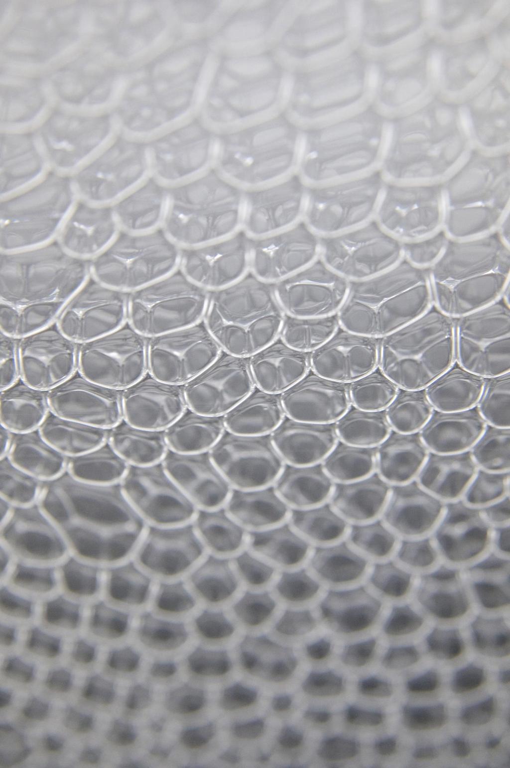
33 Chapter 2: Literature Review of film visible at the froth surface may be related to a range of underlying bubble sizes. Simulation of a monodisperse bubble sized foam resulted in a high range of polydispersity of film sizes at the froth surface. As the bubble size distribution at the froth surface may not be a sufficient indicator of the change in bubble size with height, the bubble size distribution within the froth must be fully quantified to develop accurate models of flotation. Figure 2-10: Photographs of bubbles from the pulp (left) and films at the froth surface (right) FOAMS An aqueous foam is essentially many bubbles squeezed together, where the liquid separating them is contained in a network of Plateau borders, as shown in Figure Liquid drains downwards due to gravity, the films thin leading to coalescence and the bubble size increases with height. Therefore foams are similar in structure to flotation froths. However they do not contain solids loading on the film surfaces, and require a surfactant to be created. In an aqueous foam, surfactant molecules adsorb as a monolayer on interfaces separating the gas and liquid phases. Since they are amphiphilic, they contain hydrophobic (water repelling) and hydrophilic (water attracting) tails which allow the molecule to straddle the gas/liquid boundary (Weaire & Hutzler, 1999). They improve the stability of the foam by reducing the gas/liquid surface tension, changing the visco-elasticity of the surfaces and inducing repulsive forces between the surfaces (Saint-Jalmes, 2006). Foam structure is shown in Figure 2-11: the bottom of the foam has roughly spherical bubbles with thick films separating them, but as they age the films drain, creating polyhedra with thin flat films. The bubbles increase in size due to coalescence and coarsening, but coarsening is limited by the use of gases with low diffusivity. Prof. J. Cilliers Plateau border Node Figure 2-11: Photographs of a foam showing the changes in bubble size and shape with height (left) and an aqueous foam showing key features (right). Lamella 33

34 Chapter 2: Literature Review There has been already been significant research into bubble sizing methods and foam structure measurements. These can be grouped into measurements of 3D and 2D foams D FOAMS The edge detection algorithm developed by Yang et al. (2009) to measure the bubble size distribution of the surface films of flotation froths is not useful for measuring the bubble size distribution of foams through a container wall, due to the shadows of rear films being indistinguishable from films visible at the container surface. Zabulis et al. (2007) developed a template matching algorithm to try to overcome this issue. The algorithm created a bubble prototype which evolved with different bubble sizes and rotations. However this technique has so far only been applied to spherical bubbles, and requires lengthy processing. Papara et al. (2009) studied the effect of cylindrical container diameter, wettability and base shape on the drainage of an aqueous foam by using multi modal measurements: electrical conductance for the liquid fraction, and image analysis for the bubble size distribution. With foam aging, there was a relationship between the amount of coalescence and the evolution of the liquid fraction. The largest container had the fastest drainage, despite changes in the wettability of the walls. A rounded column base stabilised the foam by increasing capillary suction effects. Cheng & Lemlich (1983) investigated errors in the measurement of foam bubble size distributions through a container wall with image analysis. A statistical sampling bias was present in the analysis, which discriminated against small bubbles. Bubbles were distorted against the column surface, so that the measured bubble size was not the actual size, and small bubbles wedged larger bubbles away from the cell surface, misrepresenting the internal bubble size distribution. In addition, the investigation showed that bubbles near a wall experience different stability conditions to those within the foam. These bubbles have fewer neighbours for bubble interactions, such as coalescence and coarsening. In general, 3D foams cannot be observed simply unless the films are very dry. In these instances other techniques have been used, such as light scattering probes (Durian et al., 1991; Vera et al., 2001) or X-ray tomography measurements (Lambert et al., 2005). However the majority of these techniques are either invasive with an effect on the foam structure; are only suitable for small, stable, foam samples; or require lengthy processing times. Foam density can be measured with electrical conductivity, as liquid can transmit an electric current and the electrical conductivities of gases, such as air, are low. Foam electrical conductivity experiments involve a number of electrodes positioned within or around a foam container. The liquid content can be calculated as the ratio of the volume of liquid contained in the foam films, Plateau borders and nodes to the total foam volume. However, to calculate the liquid content, the relationship between the electrical conductivity of the foam compared to the bulk liquid must be known. Early work by Clark (1948) showed a linear relationship between the electrical conductivity of foam and its solution, where the type of surfactant was not important in this relationship. A relationship between the electrical conductivity and liquid content in polyhedral foam was derived by Lemlich (1978), assuming that the majority of the liquid was contained in the Plateau borders, as is the case for dry foams. Electrical resistance tomography (ERT) can be used to find areas of different density within a foam, by measuring multiple signals measured from sensing electrodes placed all around an area of interest (Wang & Cilliers, 1999; Cilliers et al., 2001). Xie et 34

35 Chapter 2: Literature Review al., (2004) used ERT to measure the average bubble size in different flowing foams, as the foam density was shown to be inversely proportional to the bubble diameter in foams with Plateau borders of a certain, equal, size. Different orifices were inserted into the flowing foam column to determine the effect of air rate and orifice size on the bubble coalescence rate. This system was used to measure the dynamic behaviour of foam, but could not resolve individual bubbles. A recent review by Karapantsios & Papara (2008) highlighted an important issue with measurements based on electrical conductivity alone: that as foams evolve, their structure may change significantly without an appreciable change in the liquid content. Monnereau & Vignes-Adler (1998) developed an optical tomography system to map foam structure. After creating a stable 3D foam in a transparent column, they used a camera with a short depth of field to view consecutive slices of the foam. Each node location was recorded, so that computer visualisation of the foam structure could be reproduced with surface energy minimisation software. This visualisation was then analysed for bubble properties, such as the number of faces per bubble. However this technique was only suitable for stable foams due to the large processing times required. Ireland and Jameson (2007) measured changes in liquid transport in a dispersed two phase system. This showed that liquid fraction is a critical determinant of coalescence behaviour, but the superficial liquid velocity profiles were independent of the actual coalescence process D FOAMS Measurements of dynamic 3D foam behaviour have only been made through a transparent column wall, where only the bubbles closest to the wall are visible to image analysis methods. Additionally it has been shown that bubble behaviour is changed due to the proximity of the wall and this mode of measurement discriminates small bubbles (Cheng & Lemlich, 1983). One solution to this problem is to investigate a monolayer of bubbles. Quasi 2D foam can be created between a pair of parallel plates with a small separation; called a Hele-Shaw cell. A single layer of foam seems more limited than 3D foams, but has been shown to display important behaviour (Cox & Janiaud, 2008). Cox et al. (2002) investigated the transition of a 2D foam to a 3D foam. A bubble of volume, V, squeezed between two plates, is stable in a cylindrical configuration. If d is the distance between the plates, it has a threshold value, Equation 2-2 Past d crit the bubble deforms to a wine bottle shape, with one surface eventually pulling away from the plate and creating a hemispherical shaped bubble. This is termed a Rayleigh-Plateau instability, and this shape transition will affect the bubble neighbours, eventually creating a foam packed in 3 dimensions. The structural transition observed between the pulp and the froth in flotation, and that between spherical and polyhedral bubbles in 3D foam, corresponds to a transition from cylindrical bubbles to polygonal prisms in 2D foam. Both these shapes have constant cross sections, of circles or polygons. Their area can be readily measured from images of the foam to compare the bubble size distribution. Horizontal 2D foam behaviour has been widely investigated (e.g. Cantat et al., 2005; Dollet & Graner, 2007); these experiments are performed horizontally to reduce the effects of drainage. 35

36 Chapter 2: Literature Review Caps et al. (2006) created a vertical 2D foam in a Hele-Shaw cell by a series of inversions, or flips. The bubble size distribution of the monolayer was related to the number of flips, and bubble break ups were observed, as shown in Figure Large bubbles, such as those shown in grey, were broken up by liquid falling from above. Cox & Janiaud (2008) created a 2D foam in a vertical Hele-Shaw column to investigate liquid motion. Liquid was added to the top of the foam for forced drainage experiments. This system did not overflow. Investigations into the behaviour of a quasi 2D foam flowing horizontally around a circular obstacle in a channel have been performed by experiments and simulations. Raufaste et al. (2007) found that the yield drag, defined as the low velocity limit of the interaction force between the obstacle and the foam, was linearly proportional to the ratio of the bubble size and obstacle size, and did not depend on the channel width. A decrease in liquid fraction was associated with an increase in yield drag, as more stretched bubbles accumulated behind the obstacle at low liquid fractions. Dollet & Graner (2007) linked bubble neighbour swapping processes and bubble deformation velocity gradients in the foam flow. This revealed a complex relationship between the elasticity, plasticity and flow properties of foam. Figure 2-12: Typical bubble break up sequence recorded at 100 frames per second (Caps et al., 2006: p. 3). 2.6 BUBBLE COALESCENCE Coalescence occurs for bubbles in contact, after the liquid film separating them ruptures to form a new daughter bubble. This has a smaller lamella surface area and Plateau border length than the sum of its parents. Some of the liquid displaced by the rupture process remains in the new lamellae, to create thicker films (Cilliers et al., 2002). Surface tension acts to straighten the new lamellae, and may initiate a cascade of coalescence throughout the foam. This section will describe research into coalescence using acoustic emission and results from experiments with coalescence of bubbles created at a pair of nozzles submerged in a liquid so far the only quantified measure of bubble coalescence. Vandewalle et al. (2001) made acoustic measurements of bursting in collapsing foams. When a film ruptures, the acoustic energy that is released is proportional to its surface area. Analysis of the sound waves showed that foam collapse did not occur continuously, rather in avalanches with periods of stasis in between. The wide range of signal amplitudes showed that multiple bubble sizes were involved in each avalanche. Kracht & Finch (2009) measured the coalescence of bubbles occurring at a capillary tip using a 36

37 Chapter 2: Literature Review characteristic sound trace. With this technique, coalescence events every several milliseconds were resolved. Neethling & Cilliers (1998) found that the weir angle in a foam cell had an effect on coalescence zones, where a sloping 60 weir (from vertical) created more coalescence than a steep 30 weir. The flow profile was an additional precursor to coalescence, where different streams of bubbles colliding produced shear effects from bubble deformation. Investigations into coalescence behaviour have generally focused on bubble pair formation in liquids, either at horizontal or vertical nozzles. Such results are generally more applicable to pulp zone coalescence, however coalescence observations at the pulp/froth interface or within the froth zone are currently unattainable. They thus provide insight into coalescence mechanisms that may occur throughout the froth height. As a complete empirical model of coalescence has not yet been obtained, simplified experimental systems have been used to investigate the relationship between certain fundamental parameters. Ghosh (2009) recently reviewed all models of coalescence in liquids. These can be grouped into two categories: liquid drainage models, where coalescence is determined by the time for the film separating two coalescing bubbles to thin to the point of rupture, and stochastic models, to explain why coalescence times do not have single values in experiments. This review highlighted the importance of the surfactant adsorption behaviour at film interfaces in coalescence. Tse et al. (2003) observed binary coalescence events in the liquid phase. Some of these events produced daughter bubbles smaller than the initial bubble size. As a pair of bubbles coalesced, an annular wave of liquid initiated from the hole following film rupture, and propagated through the disappearing film. This distorted the new bubble to produce an unstable extension. They also found that larger bubbles were more prone to distortion following coalescence. A recent investigation into bubbles formed at a pair of vertical nozzles in a viscous fluid by Kazakis et al. (2008) has provided a qualitative relationship between gas flow rate, viscosity and parent bubble size. Aqueous solutions of glycerine and isobutanol were used to create the viscous liquid. As the gas flow rate was increased, a linear trend in coalescence probability was not observed. The results showed four distinct trends: in particular, the second regime for an intermediate gas flow rate had the highest coalescence probability. This occurred due to shear effects between the interfaces increasing the time for a film to drain to a critical thickness. For higher gas flow rates the coalescence probability decreased. An increase in the viscosity of the solution led to decreased drainage through the film joining the bubbles and damped the oscillation of bubble deformations after coalescence. The coalescence time was found to be inversely proportional to viscosity, with the fastest coalescence time occurring for the most viscous solution due to the greater shear stress developed. Different parent bubble sizes were created by varying the distance between the nozzles. The larger bubbles experienced severe deformations after coalescence, which continued during the bubble lifetime. By creating parent bubbles of different sizes, the angle at which bubbles approached could be investigated. This changed the drainage properties of the separating film. 37

38 Chapter 2: Literature Review 2.7 MECHANISM OF FILM RUPTURE During coalescence, the film separating two bubbles ruptures. Therefore the stability of individual films can determine the extent of coalescence. This section discusses the mechanism of rupture for the isolated film; the film separating a pair of bubbles in liquid; films contained in foams, and particle stabilised films found in flotation froths THIN FILMS Manev & Nguyen (2005) have shown that thin films have a fluctuating thickness throughout their lifetimes, with the frequency and amplitude of the discrepancies increasing with film radius. The diffusion of surfactant molecules from the bulk liquid to the interface partially compensates the surface tension gradient which prevents the outflow of liquid from the film. For thin films it accelerates the thinning process BINARY COALESCENCE IN LIQUIDS Experiments of coalescing bubbles in liquid by Tse et al. (2003) have shown an annular wave of fluid radiating away from the first point of film rupture, causing a rippling effect along the length of the bubble which may cause pinching and further rupture. A review by Craig (2004) explains that thermal disturbances cause these liquid surface waves which increase with the effect of the attractive Van der Waals forces. The superposition of these oscillations may produce a pinching effect and ultimately rupture if they have enough time to develop an amplitude similar to the thickness of the film. This is known as the capillary wave rupture mechanism (CWRM). Elasticity from the adsorbed surfactant acts to dampen these capillary waves, and thus provides an energy barrier to rupture. The only alternative proposed so far to CWRM is the process of hole nucleation, where holes in the film may spontaneously develop. The probability of their formation increases with thinning FOAMS Studies of film rupture and pairs of bubbles in the liquid phase have provided some insight into the mechanism of coalescence, but it has not yet been elucidated whether the same factors are important in foams which contain multiple bubbles and a high packing density. However, there have been few internal measurements of coalescence in foam due to the opaque nature of foam. Carrier & Colin (2003) conducted experiments with foams for free and forced drainage. These two types correspond to states where the foam is left to drain due to gravity, or where additional liquid is added to the foam to change the liquid fraction. Carrier & Colin (2003) measured the disjoining pressure exerted on foam films during rupture to be significantly less than that required to rupture an isolated film. A critical film dilatation theory was proposed as a possible cause of coalescence. This theory pronounces that foam rearrangements occur too quickly in comparison to the elastic response of the composite films. As the surfaces are stretched and drain, film rupture will occur if the time for surfactant diffusion to replenish the surfaces does not equal the time for the rearrangement FROTH FILMS Dippenaar (1982b) showed that particle stabilised films will rupture when the film thins to the particle size, where it is likely that the particle will bridge the film and destroy it. This effect can be seen in Figure 38

39 Chapter 2: Literature Review Krasowska & Malysa (2007) postulated hole nucleation as another possible source of rupture in froths. The hole is a three phase contact point which forms at the conjunction of the solid, liquid and gas phases. Figure 2-13: Diagram showing the bridging effect of particles on films, where the contact angle θ is shown for A, a hydrophilic particle and B, a strongly hydrophobic particle (Aveyard et al., 1994: p. 7). Ata (2008) investigated coalescence of pairs of loaded bubbles in a transparent liquid with high speed photography. This indicated that the role of the surfactant in film stability is different for particle stabilised bubbles, as the bubble without solids loading deformed more after coalescence. It was suggested that during the formation of flotation froths, surfactant molecules adsorbed onto the solid phase may reposition with the addition of the gas phase to stabilise the gas/liquid interface. Hydrophobicity is a surface property, and is proportional to the contact angle, θ, which is the angle a liquid film makes with a particle surface. Strongly hydrophobic particles, with a contact angle greater than 90, were found by Dippenaar (1982a) to destabilise a thin film. Johansson & Pugh (1992) postulated a peak hydrophobicity for film stabilisation. However, there is some disagreement about the specific contact angle value: Aveyard et al. (1994) suggested a value of whereas Ata et al. (2003) found the peak hydrophobicity around θ=66. Ata et al. (2003) showed that particle hydrophobicity affects froth stability in a laboratory flotation column. Hydrophilic particles with a low contact angle of 50 did not aid stability, whereas particles with an intermediate hydrophobicity (θ=66 ) created the most stable froth. Mixtures of the two were also stable, such that the more hydrophilic particles became entrained and inhibited drainage by increasing the local viscosity. They found that coalescence was increased near strongly hydrophobic particles (θ=82 ), but it still occurred with the lesser hydrophobic particles. This suggests that other mechanisms are also important in rupture, such as drainage. Since hydrophobic particles are most likely to reattach after detachment, their presence may cause a wave of film ruptures. Particle packing may affect froth stability: Ata (2008) suggested that a closely packed structure will be the most likely to resist rupture. Results of a recently published model by Morris et al. (2008) have shown that 39

40 Chapter 2: Literature Review the distance separating particles may have a stronger effect on stability than hydrophobicity. Packing arrangements can overcome the destabilising influence of particles with a large contact angle. For densely packed particles, a hexagonal packing arrangement is preferable to square packing as it requires a higher capillary pressure to rupture the film. Packing is also limited by the size and shape of the particles: Dippenaar (1982a) has suggested that irregular particle shapes would make a film more unstable. These thin film studies found that smooth glass particles required contact angles greater than 90 to rupture a film. However, cubic galena crystals ruptured a film at contact angles less than 90, as their special shape forces two 3-phase boundaries together at the same point on the particle surface. Morris et al. (2010) investigated the orientation of cubic particles in a film and their effect on the stability. Antifoam studies by Livshits & Dudenkov (1965) found an optimum particle size for coalescence. Large particles will buffer two bubbles and slow the coalescence process whereas small particles become entrained, and inhibit drainage by increasing the viscosity. Experiments by Tao et al. (2000) showed that small particles only stabilise a froth at high concentrations and have a destabilising influence at low concentrations. However, it was found that large particles always destabilised a film by increasing the onset of bridging the film. 2.8 PARTICLE MOTION IN FOAMS AND FROTHS Since the motions of different particle classes cannot be visually observed within froths as the mineral loaded bubbles are opaque, empirical research has focused on particle tracking in foams to investigate the particle motion and internal flow dynamics. The flow dynamics of the foam liquid network have already been measured by liquid dispersion in an individual Plateau border (Pitois et al., 2005); by particle dispersion in a foam under forced drainage (Lee et al., 2005), and also by particle dispersion in an overflowing foam with modified viscosity (Ata et al., 2006). Bennani et al. (2007) used Particle Tracking Velocimetry (PTV) to track particles through individual Plateau borders and nodes of a quasi-2d rising foam. By combining the PTV data with digital images, their results showed important correlations between tracer velocity and foam structure. The tracer particles achieved their maximum speed when traversing nodes and had low residence times inside Plateau borders with low angles from vertical. Ata et al. (2006) added phosphorescent tracer particles to a foam column to measure their dispersion after an injection point. Images from a CCD camera with a green filter showed changes in the liquid content profile. They added 70% by volume of glycerol to mimic the viscosity of an industrial froth while maintaining a transparent solution for analysis. However both these forms of particle tracking are limited by the need for an optically transparent system, so cannot be directly applied to flotation studies. Positron Emission Particle Tracking (PEPT) utilises pairs of back-to-back gamma-rays from positronelectron annihilation events, which can penetrate opaque surfaces, to determine the location of a radioactive tracer particle by triangulation. PEPT was developed at the University of Birmingham as a variant of the medical Positron Emission Tomography (PET) technique (Parker et al., 1993) and uses a positron camera consisting of a pair of gamma-ray detectors (Parker et al., 2002). In PEPT, a tracer particle is labelled with a positron emitting radionuclide, usually 18 F (Fan et al., 2006a; Fan et al., 2006b). The tracer is usually composed of an ion exchange resin material. During positron electron annihilation events, a pair of back-to-back gamma rays is emitted. Multiple gamma ray pairs emitted from the tracer can be detected with a positron camera and used to triangulate its position. The data logging rate of the system, which increases with tracer radioactivity, must be maximised in order to improve the signal-to- 40

41 Chapter 2: Literature Review noise ratio and provide better detection sensitivity and resolution. The tracer triangulation algorithm removes corrupt events such as from Compton scattering. The probability of tracer detection also varies with the 3D location of the tracer within the detector, where the positron camera separation is important (Guida et al., 2009). The accuracy of the technique has been validated in two ways: in the first instance, Parker et al. (2002) placed a tracer on a turntable and compared visual observations to PEPT measurements. The root mean square (r. m. s.) of the deviation of the PEPT measurement from the true path, or the spread of the data, was 0.6 mm. In the z-direction between the detectors, there was approximately 2.5 times greater uncertainty in the PEPT measurement. Parker & Fan (2008) report that for steady-state mixing, the time averaged flow pattern measured by PEPT agrees well with the instantaneous flow observed with PTV. Barigou (2004) presented a review of successful applications of PEPT to opaque mixing systems. More recently, Chan et al. (2009) observed solid particle motion in standpipes with PEPT and Guida et al. (2009) tracked particles with PEPT in a mechanically agitated solid-liquid suspension. Edwards et al. (2009) used PEPT concomitantly with Electrical Resistance Tomography, to understand aluminium hydroxide precipitation. PEPT is particularly useful for measuring foam and froth properties as the tracers can have defined surface characteristics such as size, density and hydrophobicity. The motions of hydrophilic and hydrophobic particles were measured inside a dynamic froth by Waters et al. (2008a) and Waters et al. (2008b). This showed previously unobserved particle behaviours including particle-bubble attachment, froth drop-off and re-attachment. The particle trajectory in the froth also displayed high frequency, small amplitude fluctuations superimposed on the particle motion, as shown in Figure This could not be dismissed as noise or explained due to froth structural changes as the froth and container material were completely opaque. Unexplained fluctuations Figure 2-14: Trajectory of a galena tracer particle as it moves through the froth and over the weir in different planes and views (Waters et al., 2008b: p. 4). 41

42 Chapter 2: Literature Review PEPT has already shown interesting particle behaviour within flotation froths, but this behaviour has not been verified nor quantified. This study develops methods to interpret aspects of particle trajectories measured with PEPT, and to measure particle behaviour in an overflowing 2D foam column. 2.9 SUMMARY A survey of recent literature has shown a need to quantify the mechanism and extent of coalescence throughout the froth for models of froth flotation. The bubble size entering the froth has been measured (Chen et al., 2001) along with the bubble size at the froth surface (Yang et al., 2009). However the bubble size within the froth has not been measured as the froth is fragile and opaque. Much research has focused on the bubble size distribution within foams, but this has not been without problems. Measurements of liquid fraction with electrical resistance tomography have been unable to resolve the bubble size (Xie et al., 2004). In addition, calculations of the bubble size from the measurement of liquid fraction may not be completely representative of the actual bubble size due to changes in structure occurring without a change in liquid fraction (Karapantsios & Papara, 2008). Some measurements, such as optical tomography, require stable foams to resolve the full 3D structure (Monnereau & Vignes-Adler, 1998). In addition, measuring the bubble size through a container wall is susceptible to wall effects and may not represent the internal bubble size distribution (Cheng & Lemlich, 1983). While 2D foams, or a monolayer of bubbles, behave differently to 3D foams due to the absence of lateral bubble neighbours, they present an opportunity to measure the foam properties directly through a container wall. Studies of a pair of coalescing bubbles produced at capillary tips in bubbles (Kazakis et al., 2008) provide insight into the mechanism of coalescence in liquid. However it has not yet been elucidated that the same behaviour occurs within foams or froths. Therefore the column developed in this work has a novel combination of elements: a vertical Hele-Shaw 2D foam which overflows and coalesces at a highly dynamic rate. With measurements of the bubble size, velocity and air recovery, the behaviour of the 2D flowing foam can be related to the performance of a flotation cell. This literature study has highlighted a link between cell geometry and the properties of foams and froths, such as coalescence (Neethling & Cilliers, 1998), bubble size (Papara et al., 2009) and froth motion (Zheng et al., 2004). However a comprehensive review of the effects of cell geometry on foam and froth behaviour has not been published yet. By including different inserts in the flowing foam column developed in this work, different crowder designs can be analysed in terms of the effect on bubble size, velocity and air recovery. Particle motion in the froth phase is also affected by coalescence, and requires further classification for flotation models (Neethling & Cilliers, 2002). Positron Emission Particle Tracking (Parker et al., 1993; Parker et al., 2002) can measure the behaviour of tracer particles in multiphase systems. It has already been applied to flotation froths (Waters et al., 2008a; Waters et al., 2008b), but requires further development to interpret the small detail in the trajectory of hydrophobic particles. The transparent foam column developed in this work offers an opportunity to combine PEPT trajectories and image analysis, to explain changes in the tracer trajectory. 42

43 Chapter 3: Experimental Method with Foam Columns CHAPTER 3 EXPERIMENTAL METHOD WITH FOAM COLUMNS 3.1 INTRODUCTION This chapter will detail the properties of two foam columns, which were designed, manufactured and operated to measure flowing foam behaviour with image analysis. In three phase froth systems the mineral laden films render the bubble surfaces opaque, such that nothing can be seen of the interior structure. This means that the bubble size distribution within the froth cannot be measured readily by optical methods. Two phase foams share a similar structure with flotation froths, but foams do not contain solids particles. This enables bubble size measurements with optical tomographic methods, such as in Monnereau & Vignes-Adler (1998). However many of these systems cannot resolve individual bubbles in dynamic flowing foam. The bubble surfaces are reflective and become visually opaque with several layers of bubbles. This work developed foam columns containing a single layer of foam, termed pseudo 2D, typical of a Hele-Shaw column. Therefore the bubble size distribution can be measured directly and frequently with image analysis, up to the limit of the recording frequency of high speed cameras. To better approximate flotation cells, the foams have to overflow, coalesce and burst. In this study, the columns contained a pair of internal weirs and a liquid recycle, so the foam rose in the centre of the column and overflowed on both sides. Two different sizes were used: a small column with fewer bubbles for detailed measurement of the bubble size distribution, and a large column for particle tracking. This

44 Chapter 3: Experimental Method with Foam Columns chapter begins by describing the different column properties. In order for the foam to coalesce and burst, a very specific foaming solution was developed which could be reliably measured with image analysis. Individual bubbles were tracked through image analysis so that their position, size and velocity could be compared and used to calculate the foam air recovery and average flow streamlines. These measurements will be detailed to find the steady state height, air recovery and bubble size distribution. Inserts of different size and shape were positioned in the foaming space of the overflowing foam columns to ascertain the effect of the insert geometry on the bubble size distribution, air recovery, bubble speed distribution, and streamlines. The insert geometries used in both columns will be illustrated, followed by a summary of the investigations performed in this study. 3.2 FLOWING FOAM COLUMNS A Hele-Shaw type column is composed of two vertical parallel plates, with a narrow space in between. By controlling the plate separation, a foam column with a single layer of foam can be created. With the correct separation, the bubbles form cylinders or polygonal prisms in between the plates. These prisms have a constant cross section along their axis, which is perpendicular to the column plates. This cross section can be used as a measure of the bubble area. In this work, a plate separation of 5 mm was used to create a foam with only one layer of bubbles between two Perspex plates. Two internal weirs created a foaming space and an area for the liquid from the overflowing foam to recycle. Compressed air was supplied at the base of the column and the top of the column was open to the atmosphere. Multiple PVC capillary tubes, of internal diameter mm, were arranged in a parallel configuration to ensure an even air distribution at the column base. Aeration was supplied from an air gas cylinder (purchased from BOC) attached to flowmeters operating in the ranges 0 5 l/min and 0-20 l/min. Selection of a suitable air rate and surfactant concentration produced an overflowing foam inside the column with internal coalescence and bursting at the surface. The equilibrium surface tension of each solution was measured with a MessTechnik Sita Scienceline Tensiometer t60. The viscosity of each solution was measured with an Expotech USA Model 35 Viscometer. The ambient temperature and humidity were measured with an internal room sensor. In this work two different sized overflowing Hele-Shaw columns were fabricated with specific properties to enable measurements of the bubble size distribution. The order in which the two different columns are presented in this thesis does not represent the chronological order in which experiments were conducted. The large foam column was fabricated first to provide a wider height range for coalescence to occur and to be measured with PEPT. It was composed of two Perspex plates of size 800 mm x 800 mm. The larger foaming space, size 320mm (x) and 510mm (y), contained around 6000 bubbles at the lowest air rate. The smaller column was fabricated second to measure the foam s bubble size distribution, as it contained fewer bubbles which decreased the processing time of measurements. It was composed of two Perspex plates of size 400 mm x 400 mm. The size of the foaming space was 160 mm (x) and 265 mm (y), which contained approximately 2000 bubbles at the lowest air rate. The small overflowing foam column will be described first for foam measurements, and the large overflowing foam column will be described secondly for particle motion measurements. 44

45 Chapter 3: Experimental Method with Foam Columns SMALL OVERFLOWING FOAM COLUMN (400 MM X 400 MM) A schematic of the small overflowing foam column, size 400 mm x 400 mm, is shown in Figure 3-1. It contained 16 air capillaries at the base of the column, internal diameter 1 mm, spaced every 10 mm. The pair of weirs, of width 20 mm, had outwardly angled tops. The inside surfaces of the weirs were machined and polished to a high degree of smoothness. A photograph of the small overflowing foam column is shown in Figure 3-2. The liquid recycle area contained sloping sides to minimise the liquid needed for an overflowing system at steady state. Each weir contained small gap near the column base to enable liquid from the overflowing foam to recycle. Recycle Weir Foaming Space Figure 3-1: Schematic of the small foam column, with measurements in millimetres. The plate separation is 5 mm. 45

46 Chapter 3: Experimental Method with Foam Columns Figure 3-2: Photograph of the small overflowing foam column. 46

47 Chapter 3: Experimental Method with Foam Columns LARGE OVERFLOWING FOAM COLUMN (800 MM X 800 MM) The overflowing foam was enclosed within a pair of 800 mm x 800 mm Perspex plates separated by 5mm. It contained 32 capillaries of internal diameter 1.5 mm to provide aeration at the base of the column and flat topped weirs of width 25 mm. A schematic of this system, with the weir heights and foaming space, is shown in Figure 3-3. A photograph of the experimental system is shown in Figure 3-4. Each weir contained small gap near the column base to enable liquid from the overflowing foam to recycle. Foaming Space Weir Recycle Figure 3-3: Schematic of the large foam column with measurements in millimetres. The plate separation is 5 mm. 47

48 Chapter 3: Experimental Method with Foam Columns Overflowing 2D Foam Internal Weir Solution Recycle Air Distribution Figure 3-4: Photograph of the large foam column. 48

49 Chapter 3: Experimental Method with Foam Columns 3.3 FOAMING SOLUTION It was desirable to have a surfactant used in the flotation industry, to make the results more applicable to froth flotation. The properties of the different foams were analysed visually, to find a foam that not only burst at the surface with internal coalescence, but also that overflowed and broke down rapidly after overflowing. Initially it was intended to include solid particles in the experiments, however their presence degraded the quality of captured images and the particles did not recycle completely, leading to particles clogging up lower parts of the column. A viscosity modifier was added to the foaming solution to increase the foam viscosity to a level of cp as suggested by Ata et al. (2006) to mimic flotation froths. Different surfactants were tested in the overflowing foam columns to create a suitable foam. This combination was the best compromise: a two phase system that behaved like a three phase system in terms of viscosity and remained transparent in a thin layer. It was regrettable to lose many particle effects, such as film stability, however measurement of particle behaviour was not completely removed: the motion of single particles was included with PEPT measurement. The increased viscosity also increased the Plateau border width visible at the column face. Methyl isobutyl carbinol, MIBC (Aldrich), was used as the surfactant at 2 g/l in the small column and 1 g/l in the large column. Xanthan gum (purchased from Sigma) was added at 0.1 g/l as a viscosity modifier. All solutions were prepared with deionised water, and in between experiments all equipment was rinsed with deionised water and a dilute ethanol solution (denatured, purchased from Aldrich). The effect of the xanthan gum on the two foaming solutions with different concentrations of MIBC is shown in Table 3-1. Xanthan gum had minimal effect on the surface tension of either solution. Table 3-1: Comparison of the effect of 0.1 g/l xanthan gum on the equilibrium surface tension of two foaming solutions with different concentrations of MIBC. MIBC Concentration Equilibrium Surface Tension without Xanthan gum (mn/m) Equilibrium Surface Tension with 0.1 g/l Xanthan gum (mn/m) 2 g/l Small Column g/l Large Column Xanthan gum has non-newtonian rheology, where the viscosity reduces with increasing shear rate (Whitcomb & Macosko, 1978). Song et al. (2006) express the shear rate dependent viscosity as Equation 3-1 where is the shear rate, K is the consistency index and n is the flow behaviour index. For values of n<1, the behaviour is defined as pseudoplastic. Figure 3-5 compares the measured viscosity for this system with results from Whitcomb & Macosko (1978) for the viscosity of an aqueous xanthan solution at 100 ppm. Both graphs show the expected power law trends. Table 3-2 compares the parameter values for the shear rate dependent viscosity. Both results have values of K in same order of magnitude, and values of n less than unity. The differences in the values may be attributed to the different ranges of shear rates applied. It is not possible to measure directly the shear rates present in the foam columns. 49

50 Viscosity (PaS) Viscosity (PaS) Chapter 3: Experimental Method with Foam Columns y = x R² = y = x R² = Shear Rate (s -1 ) Shear Rate (s -1 ) Figure 3-5: Graphs showing the viscosity with shear rate for a dilute (0.1 g/l) xanthan gum solution. Results from Whitcomb & Macosko (1978) are shown on the left, and the results from this work on the right. Table 3-2: Comparison of values to determine the shear rate dependent viscosity of an aqueous xanthan gum solution at 100 ppm concentration. Whitcomb & Macosko (1978) Experiment n K Shear Rate Range s s OPERATION The foaming solution was poured into the top of the column after the air at been set at the requisite level. A superficial gas velocity, J g, of 5.2 cm/s was required to provide an overflowing foam in the small foam column with 60 ml of solution. The superficial gas velocity is the ratio of the volumetric flow rate of air to the cross-sectional area of the column. The corresponding air rate for this superficial gas velocity was 2.5 l/min. The flowing foam behaviour was investigated in increments of 0.5 l/min up to a maximum of 7.5 l/min or J g = 15.6 cm/s, beyond which foam flowed out of the top of the column. The bubble size at the lowest air rate was very uniform and evenly distributed across the column width, but this changed with air rate. At the lowest air rate the bubble area was 10.5 mm 2. This bubble area was present at high air rates, however the majority of bubbles coalesced immediately after formation at higher air rates. The resultant foams had a height range of 280 to 320 mm at steady state, with a bubble size range of mm 2 from the bottom to the top of the column. This is an equivalent circular diameter of mm. For the large column, a superficial gas velocity of 5.7 cm/s was required to provide an overflowing foam with 300 ml of solution. This superficial gas velocity corresponded to an air rate of 5.5 l/min. The flowing foam behaviour was investigated in increments of 0.5 l/min up to a maximum of 9.5 l/min or J g = 9.9 cm/s, beyond which foam flowed out of the top of the column rather than overflowing the weir and collapsing. The resultant foams had a height range of 570 to 650 mm at steady state with a bubble size range of mm 2 from the bottom to the top of the column. This is an equivalent circular diameter of mm. 50

51 Chapter 3: Experimental Method with Foam Columns 3.5 FOAM MEASUREMENTS Each foam column was placed in front of a strong diffuse light source to increase the shadow of the foam Plateau borders visible to a digital camera. This was achieved with a pair of fluorescent strip lights and a diffuser screen, as shown in Figure 3-6. Images of the foam profile were captured at high resolution with a digital SLR camera, model Canon 450 EOS, at a pixel resolution of 3072 x High speed videos of the flowing foam were captured with a Casio Exilim FH20, recording at a rate of 210 frames per second and pixel resolution of 480 x 360. This camera was also used to capture a high speed, high resolution sequence at a rate of 40 frames per second. Figure 3-6: Experimental set-up in plan view. After preparing the image for analysis, the resulting images were used to measure the bubble size distribution, the bubble velocity and air recovery. This data was used to generate bubble streamlines and 2D representation of the bubble size distribution IMAGE PREPARATION Images of 2D foam contain two important characteristics: the Plateau border network and the gas cells. As an image is composed of pixels, where each pixel location is recorded as a light intensity, image processing can emphasise these two different features. The different image analysis processes used to achieve this, with their effect, are shown in Figure 3-7. The image processing software ImageJ was used (Rasband, 2008). To enable measurement of the bubble size distribution the following steps were required: 1. Reduce the image to grayscale. An image histogram shows the colour channel with the narrowest histogram peak, or lowest noise levels. In this work this was the green channel. 2. Subtract background noise and enhance the image contrast. 3. Reduce the image to binary format by thresholding, or removing pixels above a certain light level. 4. Reduce the image noise levels further, by removing light and dark outliers. Black and white inversion produces an image ready for size analysis. 51

52 Chapter 3: Experimental Method with Foam Columns 5. Obtain a list of bubble properties such as area, centre co-ordinates and perimeter with the Analyse Particles function. The recognised bubbles are shown as outlines. A combination of the outlines with the original image was used to check the validity of the bubble boundaries identified. Figure 3-7: Image processing used to segregate the Plateau border network and gas cells from an image of the foam profile. 52

53 Chapter 3: Experimental Method with Foam Columns PROPORTIONAL BUBBLE SIZE DISTRIBUTION The bubble size distribution was described in a histogram format by relating each bubble area to the initial bubble area. The bubble size distribution displayed in this way is a measure of how much coalescence has taken place over the column height, assuming all bubbles start at initial size. Two other assumptions were made: the gas has low diffusivity so the effects of diffusion can be ignored, and coalescence events did not create daughter bubbles smaller than the initial bubble area. Therefore each bubble can be represented as a multiple of the initial, or unit bubble area. The unit bubble area was estimated as an average from a sample of approximately 100 bubbles of the same initial bubble area measured with image analysis. An example of the extraction of a sample around 100 bubbles is shown in Figure 3-8. Figure 3-8: Example of extracting a sample for measuring the unit bubble size from the lower half of each image. Regarding the lower half of the column, a portion of the raw image is selected for analysis. Any bubbles not in the unit size category are removed, so that the bubble size distribution can be measured with the procedure described previously with Image J. The minimum, maximum, mean and standard deviation of the bubble areas measured can be taken from the bubble population, as shown in Table 3-3. The range of bubble areas within the sample is quite high, from 6.81 to mm 2. If the mean bubble area is used as the unit bubble size in compiling a histogram of the bubble size distribution, each class will only contain 68% of the bubbles within each unit size. For example, with the Triangle 2 measurement, using the mean of 8.67 as the unit 1 size would class all bubbles between 8.67 and as bubbles of size unit 2. From Figure 3-8, it can be clearly seen that the bubbles sampled are all of size unit 1, and therefore using 53

54 Frequency Proportion Chapter 3: Experimental Method with Foam Columns merely the mean as the unit size is incorrect. This problem would be further compounded by including bubbles of true size unit 2, in the unit 3 class, and so on, with a resulting skewed histogram. Table 3-3: Values of the minimum, maximum, mean, standard deviation and final value of the unit bubble area for the Triangle 2 insert bubble size distribution measurement. Bubble Area (mm 2 ) Minimum 6.81 Maximum Mean 8.67 Standard Deviation 0.70 Unit size at 95% confidence (μ+2σ) Therefore, assuming a normal distribution, the unit bubble area, A, was calculated at the 95% confidence limits value, Equation 3-2 where μ is the mean and σ is the standard deviation of the bubble area from the sample. The 95% confidence limits were included in the value of the unit bubble size to ensure that 95% of the population of bubbles in each unit size were included in each histogram bin. At higher air rates the population of bubbles of unit size was too small to measure with confidence, therefore the value of the unit bubble size at a superficial gas velocity of 5.2 cm/s was used. An example histogram for a superficial gas velocity of 5.2 cm/s is shown in Figure 3-9. The frequency of bubbles with areas grouped into bins of width 10.5 mm 2 is shown on the left, and the same data can be represented as the proportion of bubbles of increasing unit size, on the right. This is similar to the method of size fraction in particle sizing Bubble Area (mm 2 ) Unit Bubble Size Figure 3-9: Histogram of the bubble area (left) and the proportion of bubbles of unit size (right) for a superficial gas velocity of 5.2 cm/s. 54

55 Chapter 3: Experimental Method with Foam Columns BUBBLE AREA DISTRIBUTION OF THE FOAMING SPACE Foam images were analysed to measure the bubble area distribution across the foaming space. The lower and upper halves of the foam profile were photographed and analysed separately, to maximise the resulting pixel resolution of the images and to minimise errors from parallax. The output from image analysis was a list of measurements for each bubble, including centre co-ordinates and area. The data was interpolated into two dimensional arrays with the averageifs function in Microsoft Excel. Each bubble was represented as an area at the bubble centre point. A grid was defined with intervals at 10 mm over the column foaming space. Values of the bubble areas were averaged for any bubble centres occurring within each element. An example of this analysis is shown in Table 3-4. This form of representing the data is biased towards smaller bubbles, as larger bubbles may occupy several grid elements but are only represented in one grid element. Any grid elements that did not contain a bubble centre were given a value of the bubble area averaged from neighbouring elements. This process was repeated, for three pairs of photographs captured 0.5 seconds apart. The mean of three measurements was used to plot the average bubble area distribution with column area with the imagesc function in MATLAB. Table 3-4: Table showing an example of the data from image analysis (left), converted from pixel units to mm, and the data changed into a two dimensional array with bubble area units in mm 2. No. Bubble Centre X Y Bubble Area Y (mm) X (mm) (mm) (mm) (mm 2 ) BUBBLE VELOCITY The bubble area distribution method described in section creates a list of all bubbles, together with their area and centre co-ordinates. An algorithm was written in Matlab to calculate the velocity of a sample of bubbles between two high resolution images recorded at a rate of 40 frames per second. The distance moved by each bubble between consecutive frames was small compared to the average bubble size. For each bubble in the first frame, the algorithm searched for the nearest bubble in the second frame by comparing the bubble centre co-ordinates. The resulting distance between bubble centres in each frame was divided by the time separation between frames, seconds, to calculate individual bubble velocities. A quiver plot is shown in Figure 3-10 combined with an image of the foam, to show individual bubble velocities in between two consecutive frames. The measurement was interpolated into 55

56 Chapter 3: Experimental Method with Foam Columns a 2D format as described for bubble area in section 3.5.3, and repeated. A grid was defined with intervals at 10 mm over the column foaming space. Values of horizontal and vertical velocity were averaged for any bubble centres occurring within each element. The mean of three velocity measurements was plotted as streamlines with the MATLAB function streamslice and as a speed distribution with column area map with the imagesc function in MATLAB. The experimental streamlines are actually average bubble tracks. Figure 3-10: Sample bubble image and quiver plot combined to show the bubble velocity in pixels between two consecutive frames AIR RECOVERY The air recovery, α, of an overflowing system can be measured as (Barbian et al., 2007): Equation 3-3 where v f is the overflowing foam velocity, h w is the height of foam overflowing the weir, l is the weir lip length and Q A,in is the volumetric flow rate of gas entering the system. In this work, l corresponds to the plate separation of 5 mm. An image sequence was obtained from a high speed video of the overflowing bubble profile, where the bubble centres were approximately aligned vertically as they overflowed the weir. Two measurements were performed for each bubble with image analysis: the vertical separation between the bubble centre and the bubble centre immediately below (Δh i ), and the horizontal velocity (v h,i ) over a number of frames. For the bubble immediately above the weir, the vertical distance of the bubble centre to the weir (h 0 ) and its horizontal velocity over the weir were also measured (v h,0 ). The air recovery was therefore calculated as: Equation

57 Average Foam Height (mm) Chapter 3: Experimental Method with Foam Columns where n is the total number of bubbles in each measurement. In this work, a symmetrical overflowing profile was assumed, and the measurement from one side of the column was doubled to provide the resulting air recovery. 3.6 STEADY STATE MEASUREMENTS OF FOAM COLUMNS The columns were operated at the lowest air rate for up to 2 hours to find the steady state of the column. For the small foam column, the steady state height of the overflowing foam was found first, followed by the steady state time for the air recovery and the bubble size distribution. The steady state height of the large foam column was investigated in further detail STEADY STATE OF THE SMALL OVERFLOWING FOAM COLUMN A solution of 2 g/l MIBC and 0.1 g/l xanthan gum was used to provide an overflowing foam in the small column with J g = 5.2 cm/s. Initially the time required for the foam to achieve steady state was determined, in terms of the foam height, air recovery and bubble size distribution STEADY STATE HEIGHT The variation in the total foam height with time was measured by image analysis. At J g = 5.2 cm/s the foam achieved a steady height within several minutes, as shown in Figure High speed videos of the foam height were taken approximately every 10 minutes, after 5 minutes required to start the foam column. A sequence of 40 frames was taken from each high speed video, enabling eight measurements (one every five frames) of the foam height with image analysis. Each point was calculated as the mean of eight measurements, so that the error bars shown correspond to the 95% confidence limits on the mean calculated from the t-distribution. The dashed line corresponds to the level of the weir, so that after 100 minutes the foam no longer overflowed. The surface tension of a solution mixed at the same concentration did not change over a period of 120 minutes Time (min) Figure 3-11: Graph showing the average height with time of the small overflowing column at a superficial gas velocity of 5.2 cm/s. The top of the column is shown as a dashed line. 57

58 Unit Bubble Size (mm 2 ) Air Recovery Chapter 3: Experimental Method with Foam Columns STEADY STATE AIR RECOVERY The change in air recovery of the overflowing foam with time at an air rate of 2.5 l/min was measured using the profile method described by Equation 3-4. The error in the measurement was estimated as ±10% from the propagation of errors from each image analysis measurement involved in calculating the air recovery. The results are shown in Figure 3-12, where the air recovery was approximately constant for a period of 25 minutes. After this, it decreased to zero with time where after 120 minutes the foam no longer overflowed Time (min) Figure 3-12: Graph showing the change in air recovery with time for the small overflowing column at a superficial gas velocity of 5.2 cm/s STEADY STATE BUBBLE SIZE DISTRIBUTION The bubble size of the whole foam with time was measured with image analysis and represented in a histogram with bins according to the initial, or unit, bubble area. The change in unit bubble size used in each histogram is plotted with time in Figure This unit bubble size is the value at 95% confidence limit rather than the mean, as described by Equation Time (min) Figure 3-13: Graph showing the variation in the unit bubble size with time. The results are shown in Figure 3-14, where the bars represent the proportion of bubbles of different sizes at different times. Bubbles over a unit size of 5 were grouped together due to their low frequency. 58

59 Proportion Chapter 3: Experimental Method with Foam Columns The proportion of unit 1 bubbles decreased with time, with this effect becoming more pronounced at times over 55 minutes. The number of larger bubbles, unit 2 or greater, also increased after a time of 55 minutes. As the amount of coalescence increased with time, the foaming capacity of the solution reduced with time. Pronounced differences were seen after 45 minutes. 100% 90% 80% 70% 60% 50% 40% 30% 20% 10% 0% Time (min) Unit 5+ Unit 4 Unit 3 Unit 2 Unit 1 Figure 3-14: Graph showing the proportion of bubbles of different sizes with time for the small overflowing column at a superficial gas velocity of 5.2 cm/s. Therefore a time of 15 minutes was selected for the foam to obtain a steady height, air recovery and bubble size distribution and could be maintained for a further 10 minutes. This steady state time, having been verified experimentally for the small overflowing foam column at a superficial gas velocity of 5.2 cm/s, was used as the steady state time for higher superficial gas velocities. This assumption is reasonable for a foam with internal coalescence: Neethling et al. (2005) and Grassia et al. (2006) found that the time for foams stabilised with the surfactant Teepol to reach an equilibrium height decreased with superficial gas velocity STEADY STATE OF THE LARGE OVERFLOWING FOAM COLUMN A solution of 1 g/l MIBC and 0.1 g/l xanthan gum was used to provide an overflowing foam in the large column. The variation in the overflowing foam height with time was measured via image analysis. At the air rate of 5.5 l/min, or J g = 5.7 cm/s the foam achieved a steady height within 20 minutes, as shown in Figure High speed videos of the overflowing foam height were taken every two minutes, after the six minutes required to start the foam column. A random frame number was chosen from each video, and used to measure the overflowing foam height with image analysis. Each point after 10 minutes was calculated as the mean of three measurements, so that the error bars shown correspond to the standard deviation of these three measurements. Five points show large error bars, where the value at 14 minutes has a standard deviation corresponding to 30% of the mean. The video sequence obtained at 10 minutes was analysed further to obtain a measurement of the overflowing foam height in every 10 frames, or an interval of (10/210) seconds. The results are shown in Figure Over a period of 3 seconds the overflowing foam height fluctuated, with a repeated trend to rise for up to 0.5 seconds followed by an immediate drop off. The maximum drop 59

60 Overflowing foam height (mm) Overflowing Foam Height (mm) Chapter 3: Experimental Method with Foam Columns edge measured was 25 mm at 1.5 seconds and was due to a cascade of bursting events immediately above the weir Time (min) Figure 3-15: Graph showing the variation in the overflowing foam height in the large overflowing foam column with time, at a superficial gas velocity of 5.7 cm/s Time (s) Figure 3-16: Graph showing the fluctuation in the overflowing foam height in the large column during a period of 3 seconds at a superficial gas velocity of 5.7 cm/s. A time of 25 minutes was selected as the time required for the overflowing foam to obtain a steady height. The time for a steady air recovery and bubble size distribution are not presented as the air recovery and bubble size were not measured in the large overflowing foam column in this work. 3.7 INSERT GEOMETRIES Inserts of different size and shape were inserted into the foaming space (see Figure 3-1) of the overflowing foam columns. The inserts were composed of Perspex, with a thickness of 5 mm corresponding to the plate separation. 60

61 Chapter 3: Experimental Method with Foam Columns INSERTS IN THE SMALL OVERFLOWING FOAM COLUMN Inserts of different size and shape were positioned in the foaming space of the small overflowing foam column at superficial gas velocity 5.2 cm/s. Three rectangular inserts were used, with 2 cm, 5 cm and 8 cm width. The different depths of insertion relative to the top of the weir are shown in Figure These rectangular inserts were made with machined and polished edges, similar to the weir edges, to minimise the friction experienced by flowing foam. The insert geometry will be described according to the following example: 8x3.1 is an insert of 8 cm width at 3.1 cm depth relative to the top of the weir. Figure 3-17: Diagrams showing the different depths (mm) used with 2cm, 5cm and 8cm wide inserts in the foaming space of the small overflowing foam column. 61

62 Chapter 3: Experimental Method with Foam Columns Inserts of different shape were also used to investigate the effect on the flowing foam behaviour. The shaped inserts were made with a laser cutter; their surface was slightly different to the rectangular inserts with ridges barely visible to the eye. Their positions within the foaming space of the small foam column are shown in Figure Two inserts with triangular ends with different apex angles were inserted into the foam to create Triangle 1 with an apex angle of 90, and Triangle 2 with an apex angle of 54. The triangular shapes were 6 cm wide, inserted at depths of 5 cm for Triangle 1 and 6 cm for Triangle 2. Both the triangle ended inserts had a rectangular profile above the foaming space. Triangle 1 Triangle 2 Figure 3-18: Diagrams showing the dimensions (mm) of triangular inserts in the foaming space of the small overflowing foam column. The inserts can be described in terms of their wetted perimeter and their cross section. The wetted perimeter is the edge length of insert inside the foaming space, and the cross section is the area of insert within the foaming space. For example, the 8x12.5 insert has a wetted perimeter of (2 x 12.5) + 8 = 33 cm, and a cross section of (8 x 12.5) = 100 cm 2. Similarly, the Triangle 2 insert has a wetted perimeter of 2 x ( ) = 13.4 cm and a cross section of (6 x 6)/2 = 18 cm 2. After the foaming solution had been poured into the top of the column, and the air started, the insert was positioned centrally in the foaming space and clamped. The column was operated at 2.5 l/min, corresponding to J g of 5.2 cm/s, as this system had a uniform initial bubble size distribution. The column overflowed at this air rate with an air recovery of 0.21, leaving a range of 0.79 for improvements due to the insert design. The system was left for 15 minutes to achieve steady state. Images and high speed sequences of the foaming space were captured for image analysis measurements of the air recovery, bubble size and velocity. The unit bubble size was measured separately for each insert bubble size measurement. Examples of the foam with different inserts are shown in: Figure 3-19 for the 2 cm rectangular insert, Figure 3-20 for the 5 cm rectangular insert; Figure 3-21 for the 8 cm rectangular insert and Figure 3-22 for the triangular inserts. 62

63 Chapter 3: Experimental Method with Foam Columns Figure 3-19: Images of the small overflowing foam column with a rectangular insert of 2 cm width at various depths (cm) at a superficial gas velocity of 5.2 cm/s. 63

64 Chapter 3: Experimental Method with Foam Columns Figure 3-20: Images of the small overflowing foam column with a rectangular insert of 5 cm width at various depths (cm) at a superficial gas velocity of 5.2 cm/s. 64

65 Chapter 3: Experimental Method with Foam Columns Figure 3-21: Images of the small overflowing foam column with a rectangular insert of 8 cm width at various depths (cm) at a superficial gas velocity of 5.2 cm/s. 65

66 Chapter 3: Experimental Method with Foam Columns Figure 3-22: Images of the small overflowing foam column with different shaped inserts at a superficial gas velocity of 5.2 cm/s INSERTS IN THE LARGE OVERFLOWING FOAM COLUMN Three inserts of different size and shape were inserted into the foaming space (see Figure 3-4) of the large overflowing foam column. The inserts were composed of Perspex, with a thickness of 5 mm corresponding to the plate separation of the Hele-Shaw foam column. Two rectangular inserts were used, with 6 cm and 16 cm width. The inserts were inserted to a depth beyond the middle of the column, along a central line. The different depths of foam insertion relative to the top of the weir are shown in Figure The large foam column was operated at a superficial gas velocity of 5.7 cm/s. Photographs of the large overflowing column containing the inserts are shown in Figure The inserts were made with machined and polished edges, similar to the weir edges, to minimise the friction experienced by flowing foam. The insert geometry will be described as small, large and triangle. Positron Emission Particle Tracking Experiments in the large overflowing foam column are described in more detail in Chapter 5. 66

67 Chapter 3: Experimental Method with Foam Columns Figure 3-23: Diagrams showing the dimensions of different inserts used in the foaming space of the large overflowing foam column, with measurements in mm. The inserts were positioned at depths relative to the mid- point of the column. 67

68 Chapter 3: Experimental Method with Foam Columns Figure 3-24: Photographs of the large overflowing column with different inserts at a superficial gas velocity of 5.7 cm/s. 3.8 THE EFFECT OF AMBIENT HUMIDITY The ambient humidity of the laboratory was measured with a room sensor at the beginning of each experiment. The air recovery with humidity for an 8 cm insert at 3.1 cm depth (8x3.1) at a superficial gas velocity of 5.2 cm/s is shown in Figure The error bars correspond to the standard deviation of multiple measurements of the air recovery. Air recovery decreased with humidity. It was not possible to conduct experiments in a humidity controlled environment. All further experiments were performed with ambient humidity in the range 30-40% and ambient temperature C to minimise the effects of humidity and temperature on the air recovery. 68

69 Air Recovery Chapter 3: Experimental Method with Foam Columns Humidity (%) Figure 3-25: Graph showing the effect of ambient humidity on air recovery of the small overflowing foam column with 8x3.1 insert at a superficial gas velocity of 5.2 cm/s. 3.9 SUMMARY This work developed overflowing Hele-Shaw foam columns, where a narrow separation between two parallel plates created a pseudo-2d foam. The foam columns contained a pair of internal weirs and a liquid recycle area so that the foam overflowed on two sides. The foams achieved steady state after a certain time, which was determined by performing stability assessments over a long period of operation. The foam columns were made in two sizes, a larger one to create more detail in the overflowing foam properties and to investigate particle behaviour, and a smaller one for more efficient measurement of the bubble size and coalescence properties of the foam. A foam solution was developed as a dilute aqueous solution of MIBC to obtain an overflowing coalescing foam, and xanthan gum for increased viscosity. The resulting liquid behaved in a Non-Newtonian manner. These foam tests allow direct comparsion to a flotation cell as the foaming solution was designed to behave like a three phase flotation froth, but still actually be a two phase system suitable for image analysis measurements. The foam has a viscosity at a level found in froths; shares flow properties with flotation froths, with internal coalescence and bursting at the surface, and had geometrical aspects in common with a flotation cell, such as a weir and inserts to mimic industrial crowders. Photographs and high speed videos were captured of the foam to enable several measurements by image analysis. The bubble centres were tracked through a sequence of images, to enable calculation of the flow streamlines and air recovery. The bubble area was measured and presented as a comparison with the initial, or unit, bubble area. These measurements were applied to the small overflowing foam column at the base air rate with time to find the steady state height, air recovery and bubble size distribution. Different inserts were placed into the foam columns to change the flowing properties of the foam. Rectangular and triangular inserts of different widths were placed at different depths to investigate the effect on air recovery and the bubble size distribution. Humidity had a large effect on the air recovery. 69

70 Chapter 4: Bubble Size, Coalescence and Flowing Properties of Overflowing Foam CHAPTER 4 BUBBLE SIZE, COALESCENCE AND FLOWING PROPERTIES OF OVERFLOWING FOAM 4.1 INTRODUCTION The efficiency of a flotation froth to recover valuable mineral particles and reject gangue is closely related to the bubble size distribution through the depth of the froth. The bubble size entering the froth and the bubble size distribution at the froth surface have been measured in industry. However measurement of the bubble size within the froth is extremely difficult as the mineral laden bubble surfaces are opaque and fragile. Therefore measurement of froth interior structure cannot be achieved by optical methods. This work developed overflowing foam columns to measure the flowing properties of foam over the total column area. In this chapter, the variation in air recovery with superficial gas velocity of the overflowing foam will be determined at steady state, along with the relationship between superficial gas velocity and coalescence. The overflowing bubble velocity profile with height over the weir will be compared to the air recovery. The average bubble speed distribution will be shown to be related to the average bubble area distribution and flow streamlines. The geometry of the foam column was changed with different inserts to represent different designs for industrial crowders. Rectangular and triangular inserts were positioned in the flowing foam. After measuring the bubble velocities and sizes, the air recovery will be related to the flowing streamlines. The effect of the insert on the bubble size distribution was measured in terms of the proportions of bubbles of different sizes and their location within the foaming column.

71 Chapter 4: Bubble Size, Coalescence and Flowing Properties of Overflowing Foam 4.2 VARIATION IN AIR RECOVERY WITH SUPERFICIAL GAS VELOCITY Overflowing foams were generated in the small foam column, with a MIBC and xanthan gum solution, in order to investigate the relationship between superficial gas velocity and air recovery. Images of the overflowing small column at different values of J g are shown in Figure 4-1 and Figure 4-2. Figure 4-1: Images of the small overflowing column at different superficial gas velocities, 5.2 to 10.4 cm/s. 71

72 Chapter 4: Bubble Size, Coalescence and Flowing Properties of Overflowing Foam Figure 4-2: Images of the overflowing small column at different superficial gas velocities, 11.5 to 15.6 cm/s. 72

73 Air Recovery Chapter 4: Bubble Size, Coalescence and Flowing Properties of Overflowing Foam The air rates corresponding to each superficial gas velocity were selected at random, and the column was rinsed in between experiments. A new solution was used for each measurement and the system was allowed to run for 15 minutes in order to obtain steady state. High speed image sequences and videos were taken of the lower and upper halves of the column separately at that time. Several low resolution, but high speed (210 frames per second) image sequences were recorded for measurements of the air recovery. The air recovery of the foam overflowing the weir was calculated by Equation 3-4 using measurements of the velocity and height of every bubble over the weir. Regarding the foams in Figure 4-1 and Figure 4-2, the foam depth increases with superficial gas velocity, up to the maximum value of 15.6 cm/s. After this point the foam flowed out of the top of the column. The bubble size noticeably increases with superficial gas velocity, with fewer bubbles of unit size observed at the higher superficial gas velocities. The variation in air recovery with superficial gas velocity is shown in Figure 4-3. The error bars correspond to the 95% confidence limits of the mean calculated with the t-distribution. At superficial gas velocities lower than 12.5 cm/s the air recovery increased with J g. At values of J g of 13.5 and 14.6 cm/s, the air recovery decreased with superficial gas velocity. The highest measured air recovery occurred at 15.6 cm/s, indicating an overall trend for the air recovery to increase with superficial gas velocity. Despite two maxima in the air recovery, at an intermediate value of 12.5 cm/s and at 15.6 cm/s, a linear trend fits the data well with a value of R 2 of y = x R² = J g (cm/s) Figure 4-3: Graph showing the change in air recovery with superficial gas velocity for the small overflowing foam column. The variation in foam depth and average bubble velocity overflowing the weir with superficial gas velocity are shown in Figure 4-4 and Figure 4-5 respectively. The error bars correspond to the 95% confidence limits of the mean calculated with the t-distribution. The overflowing foam depth increased with J g up to a value of 9.4 cm/s, and after this remained approximately constant with J g, until increasing again after J g = 13.5 cm/s. The average overflowing bubble velocity also increased with J g up to 8.3 cm/s. After a drop in the average overflowing bubble velocity at J g = 8.3 cm/s, the velocity continued to increase while the overflowing foam depth remained constant. Both the average overflowing bubble velocity and foam 73

74 Overflowing Froth Depth (mm) Average Overflowing Velocity (mm/s) Chapter 4: Bubble Size, Coalescence and Flowing Properties of Overflowing Foam depth show an overall trend to increase with superficial gas velocity, resulting in the trend in air recovery that is shown in Figure 4-3. In flotation cells the drop off in air recovery after the peak is associated with a peak film stability, which is related to the particle behaviour at the film interface. This behaviour was not observed in the overflowing foam column, which contained film surfaces stabilised by a surfactant only J g (cm/s) Figure 4-4: Graph showing the variation of foam depth overflowing the weir with superficial gas velocity for the small overflowing foam column J g (cm/s) Figure 4-5: Graph showing the variation of the average overflowing bubble velocity with superficial gas velocity for the small overflowing foam column. The data illustrated in Figure 4-3, Figure 4-4 and Figure 4-5 is provided in Table A 1 in Appendix A. 74

75 Chapter 4: Bubble Size, Coalescence and Flowing Properties of Overflowing Foam 4.3 VARIATIONS IN THE BUBBLE SPEED DISTRIBUTION AND STREAMLINES WITH SUPERFICIAL GAS VELOCITY The velocity of individual bubbles at steady state was measured with image analysis in the small overflowing foam column at a range of different superficial gas velocities. By interpolating the data into two dimensional arrays, the bubble speed distribution can be plotted as a map and compared to the average flow streamlines. These results will be compared to simulations by Brito Parada (2010), involving a computational fluid dynamics model to represent froth flow in terms of a velocity potential which satisfies Laplace s equation. This model was then solved with a finite element method and applied to the geometry of the small overflowing column to obtain plots of the average velocity distribution and streamlines. The boundary conditions were defined in terms of the input air rate, bursting surface area of the foam column and the air recoveries measured at different superficial gas velocities. The experimental and simulated bubble speed distributions and average flow streamlines for J g = 5.2 cm/s are shown in Figure 4-6. The experimental data is provided in Table A 2 and Table A 3 in Appendix A. The bubble speed increased from the bottom to the top of the column with most bubbles moving at speeds of less than 100 mm/s. This implies that the bubbles accelerated with column height, particularly towards the left weir. At the centre of the column and upwards, the bubble speeds were very low. The maximum bubble speeds occurred near the side walls, with an asymmetric configuration. The bubble speeds actually in contact with the side walls were low due to friction contact forces. The average flow streamlines are all directed upwards and are quite straight. The air recovery at this air rate was This low value can be explained via Figure 4-6, as only the streamlines measured adjacent to the weir overflow, and those in the centre do not deviate towards the weir at the top of the column. The experimental and simulated streamlines are similar: all are directed upwards, with any significant horizontal deviation occurring above the weir. The simulation predicts a V-shaped section of slower bubbles at the foam surface, in agreement with the experimental speed distribution. The simulation did not predict a regions of higher bubble speeds (~120 mm/s) near the side walls. The simulation predicted the highest bubble speeds immediately over the weir, but these were not measured experimentally. However the image analysis measurement was only performed in an area of foaming space defined by the edges of the internal weir. This created partial bubble areas at the edges of the image, which were excluded from the measurements. Therefore some bubbles above the apex of the weir, where the simulation predicted high bubble speeds, were not necessarily included in the image analysis measurement. The bubble speed distribution and average flow streamlines for J g = 8.3 cm/s are shown in Figure 4-7. The experimental data is provided in Table A 4 and Table A 5 in Appendix A. In the lower part of the column, bubble speeds tended to be higher in the centre and slower near the side walls due to drag. The bubble speed distribution in the top part of the column was symmetric, with bands of areas of low and high bubble speed occurring in parallel. Areas where the streamlines compress coincide with higher bubble speeds, and areas where the streamlines expand align with lower bubble speeds. A greater number of streamlines overflowed the weir compared to J g = 5.2 cm/s in Figure 4-6, particularly over the right weir. This corresponds to a higher air recovery of 0.46 from Figure 4-3. Some streamlines do not overflow as they actually represent average bubble tracks, and may terminate in coalescence. Bubbles in the centre 75

76 Figure 4-6: Plot showing the experimental flow streamlines and average speed distribution in mm/s (left), and plot showing the simulated flow streamlines and foam velocity distribution in m/s (right), for the overflowing small column at a superficial gas velocity of 5.2 cm/s. Chapter 4: Bubble Size, Coalescence and Flowing Properties of Overflowing Foam and near the weirs had the greatest speed, with bubbles in between flowing more slowly. This caused a significant bending or horizontal deviation in the streamlines, to direct them to overflow the weir. 76

77 Figure 4-7: Plot showing the experimental flow streamlines and average speed distribution in mm/s (left), and plot showing the simulated flow streamlines and foam velocity distribution in m/s (right), for the overflowing small column at a superficial gas velocity of 8.3 cm/s. Chapter 4: Bubble Size, Coalescence and Flowing Properties of Overflowing Foam 77

78 Chapter 4: Bubble Size, Coalescence and Flowing Properties of Overflowing Foam The experimental and simulated streamlines agree, where both are straight and directed upwards. Both sets of streamlines bend over the weir, with high bubble speeds occurring in this region. The simulation predicted an area of slower bubbles at the foam surface, and this is also visible in the experimental results. The simulation underestimated the magnitude of the bubble speed in the lower part of the column, which were as high as 200 mm/s in the experimental results. The bubble speed distribution and average flow streamlines for J g = 12.5 cm/s are shown in Figure 4-8. The experimental data is provided in Table A 6 and Table A 7 in Appendix A. Bubbles near the side walls tended to be slower, with bubbles in the centre tending to be faster. The average flow streamlines show rapid changes in directionality in the lower half of the column, with areas of lower speed acting as a barrier which areas of higher speed must deviate around. This was most significant at the vertical centre of the column, where areas of high speeds were deflected towards the weirs. The average flow streamlines associated with these areas of high speed are therefore directed over the weir. Referring back to Figure 4-3, the air recovery at J g = 12.5 cm/s was The air recovery was higher at this superficial gas velocity as many streamlines are directed to overflow the weir, and bubbles travelling along these streamlines have a uniformly high speed; over 200 mm/s. The bubble speed distribution was more symmetric than measured at lower air rates. The streamlines in the upper half of the column were straighter than in the lower half, until they approached the weir. The maximum speeds measured were towards the top of the column. In comparison to the simulated streamlines, the experimental streamlines are mostly straight and directed upwards before bending over the weir. Small changes in directionality present in the lower half of the column were not predicted by the simulation. The experimental and simulated speed distributions agree in an area of lower speed at the top centre of the column and high bubble speed over the weir. However, the simulation did not predict high bubble speeds along overflowing streamlines before they approached the apex of the weir. In addition, the simulation did not predict areas of lower speed near the side walls associated with wall effects. The bubble speed distribution and average flow streamlines for J g = 14.6 cm/s are shown in Figure 4-9. The experimental data is provided in Table A 8 and Table A 9 in Appendix A. In the lower half of the column there were patches of low and high speed occurring together. The average flow streamlines were straighter in this region and tended to flow upwards, in comparison to a superficial gas velocity of 12.5 cm/s shown in Figure 4-8. In the top part of the column, the speed in the centre was higher than at lower values of J g, but the bubble speed near the side walls was lower. The speed distribution was asymmetric, with areas of very low speed (<50 mm/s) overflowing at the surface on the left side, and high speed areas (~150 mm/s) overflowing on the right. However a large number of streamlines are directed to overflow the weir, contributing to the high value of air recovery of 0.55 from Figure 4-3. Fewer wall effects were evident at this higher superficial gas velocity. 78

79 Figure 4-8: Plot showing the experimental flow streamlines and average speed distribution in mm/s (left), and plot showing the simulated flow streamlines and foam velocity distribution in m/s (right), for the overflowing small column at a superficial gas velocity of 12.5 cm/s. Chapter 4: Bubble Size, Coalescence and Flowing Properties of Overflowing Foam 79

80 Figure 4-9: Plot showing the experimental flow streamlines and average speed distribution in mm/s (left), and plot showing the simulated flow streamlines and foam velocity distribution in m/s (right), for the overflowing small column at a superficial gas velocity of 14.6 cm/s. Chapter 4: Bubble Size, Coalescence and Flowing Properties of Overflowing Foam 80

81 Chapter 4: Bubble Size, Coalescence and Flowing Properties of Overflowing Foam The area of high speed bubbles in the centre had a squeezing effect on the area of lower speed bubbles near the weir, creating a horizontal deviation similar to that at J g = 8.3 cm/s, shown in Figure 4-7. This effect is more pronounced than the reverse situation at the right weir, where an area of low speed adjacent to the weir has less deviating effect on the higher speed bubbles above. The maximum speeds measured were towards the top of the column. The simulated streamlines are in agreement with the experimental streamlines, which are mostly straight in the lower half of the column with a significant bending over the weir. The simulated bubble speed distribution was in agreement with the experimental data, with an average speed of around 180 mm/s. However, the experimental speed distribution was asymmetric, with areas of high speed occurring in the centre of the column that were not predicted by the simulations. The bubble speed distribution and average flow streamlines for J g = 15.6 cm/s are shown in Figure The experimental data is provided in Table A 10 and Table A 11 in Appendix A. The majority of the bubble speeds measured in the lower half of the column were greater than 150 mm/s, with small patches of low speed in the centre and at the base of the left wall. These areas of low speed created a horizontal deviation in the surrounding areas of high velocity.. The air recovery at J g = 15.6 cm/s was 0.73 from Figure 4-3. This higher value can be explained by coupling the large number of overflowing streamlines with the higher speed distribution at the top of the column. The speed distribution over the column was symmetric, unlike that measured for J g = 14.6 cm/s in Figure 4-9. At the lower superficial gas velocity there was a tendency for higher bubble speeds at the right side of the column, but the differences between the left and right sides of the column are less pronounced at this higher superficial gas velocity. Fewer wall effects were observed at this high superficial gas velocity. The simulated streamlines at a superficial gas velocity of 15.6 cm/s do not contain small horizontal deviations that occur throughout the column height in the experimental streamlines. The area of lower bubble speed at the foam surface predicted by the simulation was not as pronounced in the experimental data, despite having been in close agreement at lower superficial gas velocities. The decreased wall effects in the experimental bubble speed distribution are in better agreement with the simulation than at lower superficial gas velocities. The simulation predicted maximum bubble speeds over the weir, whereas in the experimental data bubbles of high speed were distributed over the column. The simulated plots are all characterised by streamlines that are parallel and vertically straight in the lower half of the column, with a symmetrical, uniformly low velocity distribution. In the top part of the column the streamlines deviate towards the weir; the extent of this deviation increases with superficial gas velocity. This behaviour was also observed in the experimental data, but small horizontal deviations in the streamlines within the foaming space were also measured. However these streamlines actually represent average bubble tracks, and are therefore subject to the effect of coalescence. The experimental bubble speed distribution was generally not as uniform as predicted by the simulations. The minimum velocities occur in the top centre of the column in the simulations, in between the overflowing sides of the column. This was observed experimentally at the superficial gas velocities 5.2, 8.3 and 12.5 cm/s. At a higher superficial gas velocity of 14.6 cm/s, the experimental speed distribution was asymmetric, resulting in high speeds in the foam top centre. At a superficial gas velocity of 15.6 cm/s, this area of low speed at the top-centre of the column was not as pronounced. The simulation and 81

82 Figure 4-10: Plot showing the experimental flow streamlines and average speed distribution in mm/s (left), and plot showing the simulated flow streamlines and foam velocity distribution in m/s (right), for the overflowing small column at a superficial gas velocity of 15.6 cm/s. Chapter 4: Bubble Size, Coalescence and Flowing Properties of Overflowing Foam experimental results differ most at the higher superficial gas velocities, implying that at higher gas flow rates the foam experiences additional effects that were not included in the simulation. 82

83 Chapter 4: Bubble Size, Coalescence and Flowing Properties of Overflowing Foam The simulated maximum velocities are confined in an area immediately above each weir, and the magnitude of this high velocity area increases with superficial gas velocity. Areas of high speed were measured above the weir at each of the superficial gas velocities, but these speeds were not the maximum speeds measured in the foam column. The experimental results show areas of equivalent maximum speed, located in the centre and near the weirs of the column. The simulated velocity distribution is approximately uniform over the column, which is markedly different to the experimental speed distribution, where many areas of areas of low and high speed occur together. In particular, the experimental speed distribution shows areas of lower speed near the side walls. This wall effect due to friction was not included in the simulations. The maximum simulated and experimental velocities at each superficial gas velocity are in agreement, as shown in Table 4-1. A superficial gas velocity of 15.6 cm/s is an exception where the simulation overestimates the maximum experimental velocity. Table 4-1: The maximum bubble speed values with superficial gas velocity for experimental and simulated data in the small overflowing foam column. J g (cm/s) Maximum Bubble Speed, Experiment (mm/s) Maximum Bubble Speed, Simulation (mm/s) In conclusion, Laplace s equation can be used to simulate the streamlines of the overflowing foam column. The simulations produced a uniform bubble speed distribution over the majority of the foaming space of the foam column, where experimental results showed areas of higher speed in the centre of the foaming space. The absence of wall effects and coalescence in the simulations is the likely cause of these differences. 4.4 VARIATIONS IN THE BUBBLE SIZE DISTRIBUTION WITH SUPERFICIAL GAS VELOCITY The bubble size distribution in the small overflowing foam column was measured with image analysis for a range of superficial gas velocities. A high resolution image sequence, recorded at 40 frames per second, was obtained for this purpose. The number of bubbles counted, the amount of coalescence, and the bubble area distribution will be looked at in further detail. The bubble size distribution data is provided in Table A 12, Table A 13 and Table A 14 in Appendix A. The total number of bubbles counted for each superficial gas velocity is shown in Figure The number of bubbles counted tended to decrease with J g. 83

84 Total Number of Bubbles Chapter 4: Bubble Size, Coalescence and Flowing Properties of Overflowing Foam J g (cm/s) Figure 4-11: Graph showing the numbers of bubbles counted in the small overflowing foam column operated at different superficial gas velocities VARIATION IN COALESCENCE WITH SUPERFICIAL GAS VELOCITY The bubble size distributions with superficial gas velocity were represented in a histogram format, so that every bubble could be compared to the initial, or unit, bubble size. The unit bubble area, as described in subsection 3.5.2, was 10.5 mm 2 for a superficial gas velocity of 5.2 cm/s. This value was also used as the unit bubble area for the higher superficial gas velocities, as the frequency of bubbles of unit size diminished rapidly with superficial gas velocity. At higher superficial gas velocities the sample size of bubbles of unit size was too small for a representative sample. Assuming that coalescence is a binary process, Table 4-2 shows the different combinations of bubbles involved in making daughter bubbles of certain unit size. Therefore bubbles of size unit 2 have only coalesced once, and two coalescence events are required to produce a daughter bubble of size unit 3 (event 1: 1+1, event 2: 2+1). Therefore the bubble size distribution, displayed as a histogram with bin corresponding the unit, or initial bubble area, can be a measure of coalescence. Table 4-2: Table showing the different combinations of parent bubbles forming daughters of unit size in binary coalescence, with the number of coalescence events corresponding to each daughter unit size. Daughter Unit Size Combinations of Coalescence Number of Coalescence Events

85 Proportion of Bubbles Chapter 4: Bubble Size, Coalescence and Flowing Properties of Overflowing Foam The variation in the bubble size distribution in the lower half of the column with superficial gas velocity is shown in Figure The data is represented in terms of the proportion of bubbles of different unit size, where any bubbles larger than unit 10 have been grouped together. At J g = 5.2 cm/s, the smallest proportion of bubbles have coalesced as the number of unit 1 bubbles is at a maximum. Additionally, less than 5% of bubbles are larger than the size unit 2, meaning that the coalesced bubbles have only been involved in one coalescence event. At J g = 10.4 cm/s, most bubbles have undergone coalescence as the number of unit 1 bubbles is at a minimum. If this value is an anomaly, the proportion of bubbles involved in coalescence events would be roughly constant from a superficial gas velocity of 9.4 cm/s and higher. However if it is not, it would imply that there is some particular film stability condition associated with the small overflowing foam column operated at this superficial gas velocity. In the lower half of the column, the proportions of bubbles at J g of 7.3 and 8.3 coalescing once are similar, as the proportions of unit 2 bubbles are similar. From the value of J g = 5.2 to 10.4 cm/s, the number of bubbles sized unit 4 to 6 increased. At a superficial gas velocity of 10.4 cm/s, 50% of bubbles have coalesced more than once, forming bubbles of size unit 3 and greater. The number of uncoalesced bubbles decreased with superficial gas velocity from 5.2 to 10.4 cm/s. At higher values of J g the number of uncoalesced, or unit 1, bubbles did not change significantly. However the proportions of bubbles of other size increased, where the number of bubbles larger than size unit 10 doubled after J g = 12.5 cm/s. 100% 90% 80% 70% 60% 50% 40% 30% 20% 10% 0% Unit 10 Unit 9 Unit 8 Unit 7 Unit 6 Unit 5 Unit 4 Unit 3 Unit 2 Unit 1 J g (cm/s) Figure 4-12: Chart showing the proportion of bubbles of different unit size in the lower half of the small overflowing column operated at different superficial gas velocities. The variation in the bubble size distribution in the upper half of the column with superficial gas velocity is shown in Figure The least amount of coalescence occurred at J g = 5.2 cm/s, as in the lower half of the column. However at all other superficial gas velocities, at least 80% of the bubbles had coalesced at least once by the time they reached the upper half of the column. The proportion of bubbles coalescing once, corresponding to a bubble size of unit 2, remained roughly constant between the values of J g

86 Proportion of Bubbles Chapter 4: Bubble Size, Coalescence and Flowing Properties of Overflowing Foam and 12.5 cm/s. The proportion of bubbles coalescing three times or more, corresponding to bubbles sized unit 4 and above, increased to 50% at superficial gas velocities of 9.4 and 10.4 cm/s. 100% 90% 80% 70% 60% 50% 40% 30% 20% 10% 0% Unit 10+ Unit 9 Unit 8 Unit 7 Unit 6 Unit 5 Unit 4 Unit 3 Unit 2 Unit 1 J g (cm/s) Figure 4-13: Chart showing the proportion of bubbles of different unit size in the upper half of the small overflowing column operated at different superficial gas velocities. At high superficial gas velocities, 13.5 cm/s and above, the proportion of bubbles coalescing many times increased, with the proportions of bubbles sized unit 6 and upwards at least 30%. Between the values of J g of 5.2 and 8.3 cm/s, the proportion of bubbles size unit 10 and above increased. Between the values of J g of 9.4 and 12.5 cm/s the proportion of bubbles with size unit 10 and above was roughly constant, with the smallest proportion at 12.5 cm/s. At the higher superficial gas velocities, 13.5 to 15.6 cm/s, the amount of bubbles with size over unit 10 was over 10%. The bubble size distributions from the lower and upper halves of the column are combined in Figure Overall, the amount of coalescence increased between the superficial gas velocities 5.2 and 8.3 cm/s, as a result of the increase in bubbles coalescing twice or more. An intermediate superficial gas velocity of 10.4 cm/s had a bubble size distribution with the greatest proportion of coalesced bubbles. Values of J g of 11.5 and 12.5 cm/s had comparable levels of coalescence, with similar amounts of bubbles of different unit size. At superficial gas velocities over 12.5 cm/s, the bubble size distributions tended to have larger bubbles, with 15.6 cm/s having the largest number of bubbles coalescing three times or more. A superficial gas velocity of 15.6 cm/s was associated with an additional increase in air recovery after a decrease in air recovery from 12.5 cm/s, shown in Figure 4-3. The proportion of bubbles over size unit 10 was the highest at 15.6 cm/s, and the proportion of bubbles coalescing three or more times was 25%. The air recovery at J g = 15.6 cm/s was 8% higher than at 12.5 cm/s, but this increase had an effect on the bubble size distribution. Between the superficial gas velocities 12.5 cm/s and 15.6 cm/s, the proportion of total coalesced bubbles did not change significantly, however the number of coalescence events 86

87 Proportion of Bubbles Chapter 4: Bubble Size, Coalescence and Flowing Properties of Overflowing Foam increased with increased proportions of larger bubbles. If this data represented the bubble size distribution of a industrial flotation system, the improvement in air recovery between superficial gas velocities of 12.5 and 15.6 cm/s would not be justified due to the increase in bubble size. The increased proportion of coalescence would diminish flotation efficiency by causing a decrease in recovery of attached valuable mineral particles. 100% 90% 80% 70% 60% 50% 40% 30% 20% 10% 0% Unit 10+ Unit 9 Unit 8 Unit 7 Unit 6 Unit 5 Unit 4 Unit 3 Unit 2 Unit 1 J g (cm/s) Figure 4-14: Chart showing the proportion of bubbles of different unit size for the total area of the small overflowing column operated at different superficial gas velocities VARIATION IN BUBBLE AREA DISTRIBUTION WITH SUPERFICIAL GAS VELOCITY The bubble area distribution in the small overflowing column at different values of J g was interpolated into a 2D format. By comparing the bubble speed and size distributions over the foaming space, the effect of the bubble speed distribution on the bubble area distribution can be found. The experimental data for the figures in this subsection is provided in Table A 15, Table A 16, Table A 17, Table A 18 and Table A 19 in Appendix A. The average bubble area distribution and flow streamlines for the small overflowing column at different superficial gas velocities can be seen in Figure At a superficial gas velocity of 5.2 cm/s the bubble area distribution was asymmetric, with a tendency for larger bubbles to be on the left hand side of the column. For a superficial gas velocity of 8.3 cm/s, the top centre area containing large bubbles occurred immediately after a high speed area, as shown in Figure 4-7, which contained small bubbles. Bubble area increases were only measured at the top of the column. At a superficial gas velocity of 12.5 cm/s, bubble area increases started at the bottom of column, with two bands of larger bubbles aligned with compressed streamlines that overflowed the weir. The bubble area was constant along these streamlines until they reached the weir, despite initiating with a larger bubble area of approximately 100 mm 2. 87

88 Chapter 4: Bubble Size, Coalescence and Flowing Properties of Overflowing Foam Figure 4-15: Average bubble size distribution (in mm 2 ) and flow streamlines for the overflowing small column at different superficial gas velocities (cm/s). 88

89 Chapter 4: Bubble Size, Coalescence and Flowing Properties of Overflowing Foam At a superficial gas velocity of 14.6 cm/s, the bubble area distribution was asymmetric, as was the speed distribution as shown in Figure 4-9. Two bands of larger bubbles started in the bottom of the column along overflowing streamlines. In comparison to J g = 12.5 cm/s where the bubble area remained constant along streamlines of higher velocity, at J g = 14.6 cm/s the bubble area increased along the equivalent streamlines. At a superficial gas velocity of 15.6 cm/s, there were few bubbles of initial size, implying that the bubbles coalesced immediately after formation. The areas of small bubbles coincide with areas of low speed, as shown previously in Figure The areas of larger bubbles coincide with areas of high speed. At higher superficial gas velocities, large bubbles broke up and coalescence events produced daughter bubbles smaller than the initial bubble area. These behaviours were observed by Caps et al. (2006) in a inverting Hele-Shaw foam column and Tse et al. (2003) for a pair of bubbles in a liquid phase, respectively. Generally, the average bubble area increased with column height, and the proportion of smaller bubbles decreased with superficial gas velocity. The largest bubble area measured was at a superficial gas velocity of 15.6 cm/s. Bubble size increases often coincided with areas where streamlines were compressed together, or spread apart. The bubble area distributions at each superficial gas velocity showed larger bubbles in a V shape at the top of the column, which is an area which coincides with bubble stretching at the surface. This occurs when bubble streamlines are spread apart as bubbles near the weir overflow. 4.5 GEOMETRY INVESTIGATION Different inserts were placed in the small overflowing foam column in order to investigate the effect of insert size and shape on the resulting flowing foam properties. The results will provide insight into different crowder designs used to maximise the overflowing froth properties on industrial flotation cells. Air recovery in industrial flotation cells is associated with metallurgical performance, in particular the recovery of attached and entrained particles. Excessive coalescence results in a lower recovery of attached particles, therefore the optimum column geometry will have high air recovery and modest levels of coalescence. As described in section 3.7.1, rectangular inserts of different width were positioned at different depths in the foam to find the effect on air recovery and coalescence. Triangular inserts were also tried. Several cases were studied in further detail: three rectangular inserts with equivalent area but different width and depth; an insert with high width and depth, and a triangular insert. Images of the flowing foams were analysed to find the bubble size and speed distributions, and their relationship with average flow streamlines VARIATION IN AIR RECOVERY WITH INSERT GEOMETRY High speed sequences of the flowing foams were captured for measurement of the bubble velocity and height above the weir. Several measurements were made for each insert, each of a stack of bubbles with aligned centres as they overflowed the weir. These measurements were used to calculate the air recovery with Equation 3-4. Each set of measurements was repeated at least three times to find the mean air recovery. This section will present the air recovery calculated for rectangular inserts first, followed by shaped inserts. The data illustrated in this section in provided in Table A 20 in Appendix A. 89

90 Air Recovery Chapter 4: Bubble Size, Coalescence and Flowing Properties of Overflowing Foam The effect of insert width for different depths on the air recovery of a small overflowing foam column at J g = 5.2 cm/s is shown in Figure The error bars correspond to the standard deviation in the mean air recovery for each insert. The standard deviation of the mean air recovery was often large, due to a high range of variability in the measurements of the air recovery. It would be logical to expect the air recovery to increase with insert width, as increasing the insert width would be continually reducing the area at the top of the column through which the foam flows. Within the limits of the error bars, there is a trend for the air recovery to increase with insert width shown in Figure However it does not appear to be uniform with depth and shape. The rectangular insert with the greatest effect on the air recovery was an 8 cm wide insert at a depth of 12.5 cm. It improved the air recovery of the system compared to no insert approximately twice to 0.68 by removing a quarter of the total foaming space. However, narrower inserts at a depth of 12.5 cm had very little effect on the air recovery. At a depth of 3.1 cm, the air recovery increased linearly with insert width, with the most pronounced effect with the 8 cm width insert. At depths of 5 cm and 8 cm, none of the inserts had a significant effect on the air recovery with only small increases. The Triangle 1 insert had a similar effect on the air recovery as the rectangular inserts of comparable width and depth. The Triangle 2 insert increased the air recovery to a similar level of the 8x12.5 insert, despite being of lesser width and depth. In this instance, shape is obviously a determining factor in the air recovery behaviour. The Triangle 1 insert looks like a rectangular insert at the top of the weir, with its triangular shaped portion lower in the column, and it has an air recovery within the limits of a rectangular insert of the same width and depth. The Triangle 2 insert has a triangular shape up to the point of the weir, and therefore has a much stronger influence on the flow direction No Insert 12.5 cm Depth 8 cm Depth 5 cm Depth 3.1 cm Depth 1.9 cm Depth Triangle 1 Triangle Insert Width (cm) Figure 4-16: Graph showing the variation in air recovery with insert width for different insert widths in the small overflowing foam column at a superficial gas velocity of 5.2 cm/s. 90

91 Air Recovery Chapter 4: Bubble Size, Coalescence and Flowing Properties of Overflowing Foam The effect of insert depth on the air recovery for different insert widths in the small overflowing foam column at J g = 5.2 cm/s is shown in Figure The error bars correspond to the standard deviation in the mean air recovery for each insert. Overall the 2 cm width insert had little effect on the air recovery within the limits of the error bars. The 5 cm width insert increased the air recovery by at least 50% at shallow depths, from 1.9 cm to 3.1 cm depth. However at depths beyond 5 cm this effect reduced, culminating in a negative effect on the air recovery at 12.5 cm depth. The 8 cm width insert doubled the air recovery at shallow depths, but this effect decreased with depth to a minimum at 8 cm depth. At a depth of 8 cm, all inserts had a similar effect on the air recovery, implying that the insert width was not an important insert property in the air recovery. The effect of the 8 cm width insert on air recovery increased with insert depth after 8 cm depth, with a maximum at 12.5 cm depth despite removing a quarter of the total foaming space in this configuration No Insert 2 cm Width 5 cm Width 8 cm Width Triangle 1 Triangle Insert Depth (cm) Figure 4-17: Graph showing the variation in air recovery with insert depth for different insert widths in the small overflowing foam column at a superficial gas velocity of 5.2 cm/s. The Triangle 1 insert had a small positive effect on the air recovery, but this was similar in magnitude to the rectangular inserts at the same depth, 5 cm. This implies that the insert depth was more important than the insert shape at intermediate depths. The Triangle 2 insert had a large effect on the air recovery, raising it to 0.68 compared to 0.29 with no insert. The rectangular inserts between a depth of 5 and 8 cm did not have any large effect on the air recovery: therefore as the Triangle 2 insert was positioned at a depth of 6 cm, this implies that the shape of the insert was the determining factor in the air recovery. The effect of inserts of different wetted perimeter on the air recovery of the small overflowing column at J g = 5.2 cm/s is shown in Figure 4-18 with lines of constant depth. The 2 cm insert was designated with coloured triangle symbols, 5 cm with coloured diamonds and 8 cm with coloured squares. The triangular inserts are shown as grey and white triangles. The path by which a bubble travels to overflow the weir should be related to the wetted perimeter, as bubbles in contact with the insert must pass around the 91

92 Air Recovery Chapter 4: Bubble Size, Coalescence and Flowing Properties of Overflowing Foam insert perimeter to reach the foam surface, and bubbles nearby are influenced by this trajectory. In the small overflowing foam column, the air recovery tended to increase with wetted perimeter at low depths. The insert width provides the greatest component to the wetted perimeter at shallow depths, and therefore determines the air recovery. The main effect of the width of the rectangular inserts is to reduce the area by which foam may leave the column, and can increase the air recovery by forcing bubbles to rise near the weir where it is more likely they will overflow. The extent of this effect was an increase in air recovery of around 50%. The lowest width inserts generally did not have any effect on the air recovery as the width did not reduce the foam surface significantly. The width 2 cm corresponds to the diameters of two bubbles, so the insert will not influence the path of many bubbles. This effect is at a maximum air recovery around 13 cm, with the 8x3.1 insert, which has enough width to force foam over the weir but not enough depth to interfere with the foam below. The Triangle 2 insert had a greater effect, partly due to its moderately high width, but more importantly due to its shape. The angled sides directed foam away from the foam surface and towards the weir. Further the angle of the triangle sides is important too, as the Triangle 2 insert, with an apex angle of 54 and width and depth 6 cm, raised the air recovery to 0.69 from 0.29 with no insert. This was approximately twice the effect of the Triangle 1 insert, with an apex angle of 90, width 6 cm and depth 5 cm, even though both inserts had similar wetted perimeters Insert Wetting Perimeter (cm) No Insert 8 cm x 12.5 cm 8 cm x 8 cm 8 cm x 5 cm 8 cm x 3.1 cm 8 cm x 1.9 cm 5 cm x 12.5 cm 5 cm x 8 cm 5 cm x 5 cm 5 cm x 3.1 cm 5 cm x 1.9 cm 2 cm x 12.5 cm 2 cm x 7.8 cm 2 cm x 3.1 cm Triangle 1 Triangle 2 Figure 4-18: Graph showing the variation in air recovery with insert wetted perimeter with lines of constant depth, for a range of inserts in the small overflowing foam column at a superficial gas velocity of 5.2 cm/s. After this maximum, the air recovery then decreased with increasing wetted perimeter. As the wetted perimeter increased, the insert depth increased to become the larger component in the wetted perimeter. It is likely that the increased insert depth provides more distance for the bubbles to straighten their path, and therefore burst at the surface near the insert rather than be directed towards the weir. This effect was at a minimum around cm for the 2 and 5 cm inserts at a depth of 12.5 cm. However the second maximum in the air recovery does not fit with this interpretation: at a wetted 92

93 Air Recovery Chapter 4: Bubble Size, Coalescence and Flowing Properties of Overflowing Foam perimeter of 33 cm, corresponding to the 8x12.5 insert, the air recovery was The high value may be a result of the combination of the width and depth effects described previously: the increased cross section of the column may be the reason for the increased air recovery with the 8x12.5 insert. The reason could not be width alone as the 8 cm width insert had less effect on the air recovery at intermediate depths, and it could not be solely depth as the 2 cm and 5 cm inserts at 12.5 cm depth had the lowest values of air recovery. The effect of inserts of different cross-sectional area on the air recovery of the small overflowing foam column at J g = 5.2 cm/s is shown in Figure The 8x12.5 insert had the highest cross-sectional area and the greatest air recovery. This can be explained by the large cross-section significantly reducing the foam volume in the centre of the column, as here bubbles at the surface are furthest away from the weir and therefore least likely to overflow. However, despite occurring at different ends of the insert cross-section range, the 8x12.5 and Triangle 2 inserts had the same effect on the value of the air recovery: the maximum with the Triangle 2 insert was at 18 cm 2 and the 8 x 12.5 cm insert was at 100 cm Insert Cross Section (cm 2 ) No Insert 8 cm x 12.5 cm 8 cm x 8 cm 8 cm x 5 cm 8 cm x 3.1 cm 8 cm x 1.9 cm 5 cm x 12.5 cm 5 cm x 8 cm 5 cm x 5 cm 5 cm x 3.1 cm 5 cm x 1.9 cm 2 cm x 12.5 cm 2 cm x 7.8 cm 2 cm x 3.1 cm Triangle 1 Triangle 2 Figure 4-19: Graph showing the variation in air recovery with insert area with lines of constant depth, for a range inserts in the small overflowing foam column at a superficial gas velocity of 5.2 cm/s. The different insert depths were selected at the beginning of the geometry investigation to enable direct comparison between the cross-sectional area of different widths of rectangular insert. For example, at an insert cross-sectional areas of 40 cm 2, the 5x8 and 8x5 geometries had a similar, small effect on the air recovery. The geometry combinations 8x1.9 and 5x3.1 also had very similar insert cross-sectional areas: 15.2 cm 2 and 15.5 cm 2. They had similar positive effects on the air recovery, compared to the air recovery with no insert. However, the 2x7.8 insert also has a similar cross-sectional area of 15.6 cm 2, and had little effect on the air recovery. Furthermore, the range of air recoveries for inserts with cross-sectional area around 25 cm 2 was quite high: 8x3.1 doubled the air recovery; 5x5 increased by a lesser amount of 75% and had the 2x12.5 insert had a slight negative effect on the air recovery. 93

94 Chapter 4: Bubble Size, Coalescence and Flowing Properties of Overflowing Foam Therefore, the results in this section have indicated that at shallow depths, a high insert width leads to a high air recovery. However, at intermediate depths the increase in the insert wetted perimeter leads to a decrease in the air recovery and any benefits from increasing the width are lost. The effects of width and depth at intermediate range are potentially less important than insert shape as the Triangle 2 insert produced a high air recovery. This effect can be attributed to the angled sides of the insert directing bubble paths towards the weir. At high depths, narrow inserts had no effect on the air recovery, whereas an 8cm width insert produced a maximum air recovery. This insert combination had a high cross-sectional area, however the other inserts did not show any strong trend between air recovery and cross-sectional area. The high air recovery is a likely a result of the large insert cross-section removing the area of the foam surface which is normally associated with bursting rather than overflowing the weir. It is worth noting that nearly all of the inserts had a positive effect on the air recovery VARIATIONS IN BUBBLE SPEED DISTRIBUTION AND STREAMLINES WITH INSERT GEOMETRY Five different insert combinations were analysed further to compare the bubble speed distribution with column area and average flow streamlines. The data was interpolated into a 2D format with the averageifs function in Microsoft Excel. The five insert geometries investigated were 2x12.5, 5x5, 8x3.1, 8x12.5 and Triangle 2. The experimental streamlines and speed distribution of the column with different inserts were compared to the model developed by Brito Parada (2010). This was developed to represent foam flow in terms of a velocity potential which satisfies Laplace s equation. The average bubble speed distribution and flow streamlines for the 2x12.15 insert in the small overflowing foam column is shown in Figure The experimental data is provided in Table A 21 and Table A 22 in Appendix A. Referring back to the average speed distribution and average flow streamlines at J g = 5.2 cm/s with no insert, Figure 4-6 showed an small increase in speed from the bottom to the top of the column. The streamlines were mostly straight, with minor deviations at the top towards the weir. In the lower half of the column with the 2x12.5 insert, the average bubble speed was generally higher than in the column without insert. The base of the insert created horizontal deviations in the nearby average flow streamlines, with decreasing effect on streamlines towards the weir. The streamlines that were deviated by the insert towards the weir, actually ended up straightening or even deviating towards the insert at the foam surface. This confirms the idea mentioned in the previous section, that due to the great insert depth, the streamlines deviated by the insert had sufficient distance to straighten before reaching the foam surface. The deviating influence of the insert was therefore lost, and did not lead to an increase in air recovery. The bubble streamlines in contact with the insert experienced an additional drag force, and the average bubble speed in this area was lower. The streamlines were also compressed in between the weir and insert, but only the two streamlines closest to the weir overflowed. For the 2x12.5 insert, the simulated streamlines are strong agreement with the experimental streamlines, in terms of being mostly straight with deviation around the base of the insert and overflowing the weir. The simulated and experimental average bubble speed distributions are similar, where they agree on the bubble deceleration between the insert and side wall and areas of low speed at the base and top of the insert. They differ in the absence of wall effects in the simulated data, and the presence of increased bubble velocity above the weir and at the insert corners. 94

95 Figure 4-20: Plot showing the experimental (left, mm/s) and simulated (right, m/s) flow streamlines and average bubble speed distribution with the 2x12.5 insert in the small overflowing foam column at a superficial gas velocity of 5.2 cm/s. Chapter 4: Bubble Size, Coalescence and Flowing Properties of Overflowing Foam 95

96 Chapter 4: Bubble Size, Coalescence and Flowing Properties of Overflowing Foam The effect of the 5x5 insert on the average bubble speed distribution and average flow streamlines in the small overflowing foam column at J g = 5.2 cm/s is shown in Figure The experimental data is provided in Table A 23 and Table A 24 in Appendix A. The thin strip of 0 values to the left of the insert are a result do not respond to measure bubble speeds, rather the grid elements are empty. The 5x5 insert increased the air recovery to 0.43 from 0.29 compared to the column with no insert. This increase can be explained by the bubble acceleration in between the insert and weirs and the increased number of overflowing streamlines due to the presence of the insert. In the lower half of the column, the average bubble speed was higher with the 5x5 insert compared to the column without insert. In the upper half of the column, the insert created horizontal deviations in the streamlines around the base of the insert. The extent of this deviation was greater than with the 2x12.5 insert, however the streamlines nearest to the insert did not overflow. The average bubble speed was at a maximum along these streamlines, however as they did not overflow, their increased velocity did not contribute to an increase in the air recovery. At the base of the insert, the average bubble speed was lower, implying that bubbles decelerated upon coming into contact with the insert. The average bubble speed overflowing the weir was higher than with the 2x12.5 insert, therefore resulting in a higher air recovery. With the 5x5 insert, the average bubble speed in the column was generally underestimated by the simulation in comparison to the experimental data. The experimental average bubble speed in between the insert and the weirs approaches 150 mm/s, whereas the simulated average bubble speed approaches 90 mm/s towards the top of the column. In addition, the high bubble speeds along streamlines adjacent to the insert were not predicted by the simulation. However, the simulation and experiment did agree in the acceleration around the insert corners, and in the size of the low speed area underneath the insert. The experimental streamlines were predicted by the simulation, particularly in the degree of horizontal deviation around the base of the insert and over weir. The average bubble speed distribution and flow streamlines in the small overflowing foam column with the 8x3.1 insert at J g = 5.2 cm/s are shown in Figure The experimental data is provided in Table A 25 and Table A 26 in Appendix A. The air recovery of this system was approximately double the value of the column with no insert; 0.62 compared to The average bubble speed at the bottom of the column was higher than in the column without insert, however these bubbles decelerated towards the centre of the column. In the upper half of the column, bubbles accelerated towards the base of the insert and then decelerated after colliding with it. The area of low speed under the insert was larger than that observed with the 5x5 insert in Figure Maximum speeds occurred around the corners of the insert, but the bubbles then decelerated slightly before overflowing. The insert created large horizontal deviations in the streamlines around the base of the insert. As the insert was inserted at a shallow depth in the foam, the streamlines did not straighten very much before reaching the foam surface. The number of overflowing streamlines and average bubble speed over the weir were both higher than observed for the column with and without other inserts, resulting in the higher value of air recovery. 96

97 Figure 4-21: Plot showing the experimental (left, mm/s) and simulated (right, m/s ) flow streamlines and average bubble speed distribution with the 5x5 insert in the small overflowing foam column at a superficial gas velocity of 5.2 cm/s. Chapter 4: Bubble Size, Coalescence and Flowing Properties of Overflowing Foam 97

98 Figure 4-22: Plot showing the experimental (left, mm/s) and simulated (right, m/s) flow streamlines and average bubble speed distribution with the 8x3.1 insert in the small overflowing foam column at a superficial gas velocity of 5.2 cm/s. Chapter 4: Bubble Size, Coalescence and Flowing Properties of Overflowing Foam 98

99 Chapter 4: Bubble Size, Coalescence and Flowing Properties of Overflowing Foam The simulated average bubble speed distribution with insert 8x3.1 generally agrees with the experimental equivalent. The bubble streamlines were similar in both experiment and simulation, including the straightening effect of the insert depth of 3.1 cm. The experimental and simulated bubble speed distributions also agreed on the zone of low bubble speeds near the base of the insert. In the simulation, the areas of high speed are localised to the corners of the insert and immediately above the weir. Areas of high speed also occurred here in the experimental data, but the areas encompassed the entire space between the insert and the weir. The bubble acceleration before collision with the base of the insert or at the bottom of the column were not predicted in the simulated average bubble speed distribution. The average bubble speed distribution and flow streamlines in the small overflowing foam column with insert 8x12.5 are shown in Figure The average bubble speed in the lower half of the column was higher than in the column with no insert, from Figure 4-6. As the streamlines approached the insert base, they did not deviate around the insert corners as much as observed previously for the 8x3.1 insert, in Figure There was an area of lower speed directly underneath the insert, as observed with all the inserts in this section. In the upper half of the column, the bubbles accelerated between the weir and the insert to around 200 mm/s, with very few areas of low bubble speed. The high value of air recovery, 0.68, is a result of the high bubble speeds in between the weir and insert, despite the apparent low number of overflowing streamlines. The average bubble speed distribution was underestimated by the simulation, as it did not predict the magnitude of the bubble acceleration in between the insert and the weir. However the simulation did predict the areas of high average bubble speed near to the corners of the insert. The The simulated flow streamlines with the insert 8x12.5 are similar to the experimental streamlines, however small horizontal perturbations are present in the experimental streamlines. This may be due to coalescence, which was not included in the simulations. The average speed distribution and flow streamlines for the small overflowing foam column with insert Triangle 2 at J g = 5.2 cm/s are shown in Figure The experimental data is provided in Table A 29 and Table A 30 in Appendix A. The average bubble speed distribution was very similar to that of the rectangular inserts, with one major exception: the area of lower speed underneath the insert was much smaller at the triangle apex. The horizontal deviation in the streamlines induced by the triangular insert was more gradual and uniformly distributed between the insert and the side walls. There was less acceleration in between the insert and side wall than compared to the inserts 8x3.1 and 8x12.5, and the average bubble speed was much lower. However the air recovery was of equivalent magnitude to those rectangular inserts with the Triangle 2 insert, thus agreeing with the idea from the previous section that the triangle shape of the insert deviated the bubbles over the weir. The rectangular portion of the insert above the triangle shape reduced the number of overflowing streamlines, as some adjacent to the insert did not overflow. 99

100 Figure 4-23: Plot showing the experimental (left, mm/s) and simulated (right, m/s) flow streamlines and average bubble speed distribution with the 8x3.1 insert in the small overflowing foam column at a superficial gas velocity of 5.2 cm/s. Chapter 4: Bubble Size, Coalescence and Flowing Properties of Overflowing Foam 100

101 Figure 4-24: Plot showing the experimental (left, mm/s) and simulated (right, m/s) flow streamlines and average bubble speed distribution with the Triangle 2 insert in the small overflowing foam column at a superficial gas velocity of 5.2 cm/s. Chapter 4: Bubble Size, Coalescence and Flowing Properties of Overflowing Foam 101

102 Average Bubble Area (mm 2 ) Chapter 4: Bubble Size, Coalescence and Flowing Properties of Overflowing Foam The simulation again underestimated the average bubble speed distribution in between the insert and weir for the Triangle 2 insert. The experimental average bubble speed distribution did not show the same level of acceleration immediately over the weir and also showed an area of deceleration below the weirs. This area of deceleration is likely to be a result of the streamlines deviated by the insert toward the weir, restricting the path of streamlines rising directly from below adjacent to the side wall. The degree of deviation in the experimental streamlines was predicted by the simulation, along with the areas of low speed at the triangle apex and at the foam surface adjacent to the insert. In summary, the foam flow simulation with Laplace s equation did predict the streamline behaviour observed in the experimental data for a range of different inserts. However the average speed distribution in between the weir and in the insert was generally not predicted well by the simulation, with the maxima occurring in different locations VARIATION IN COALESCENCE WITH INSERT GEOMETRY The bubble size distribution of the small overflowing foam column with a range of different inserts was measured at steady state. High resolution images at 40 frames per second were recorded to enable image analysis measurements. The initial, or unit 1, bubble area was measured with each insert and used as the bin width to represent the data in a histogram format. In this way, the amount of coalescence and the resulting bubble areas were determined for each insert. The data illustrated in this subsection is provided in Table A 31 in Appendix A. The initial bubble areas used as the unit bubble size for different inserts are shown in Figure The unit size remained roughly constant with insert width and depth. The unit bubble size for the column without insert was measured again, at the same time as the other insert tests in the small overflowing foam column. The value was higher than measured at a superficial gas velocity of 5.2 cm/s for analysis of the bubble area distribution variation with superficial gas velocity in section This difference can be attributed to the Perspex panels of the column stretching with the frequent addition and removal of the inserts. As the tests varying the superficial gas velocity were performed prior to the insert tests, their results have not been influenced by the damage to the Perspex panels Insert Depth (cm) 2cm Width 5cm Width 8cm Width No Insert Triangle 1 Triangle 2 102

103 Total Number of Bubbles Chapter 4: Bubble Size, Coalescence and Flowing Properties of Overflowing Foam Figure 4-25: Graph showing the variation in the area of the unit bubble measured in the small overflowing foam column with different inserts. The total number of bubbles for rectangular inserts of different width with depth is shown in Figure Over the total column, the number of bubbles decreased with insert depth and width. The Triangle 2 insert contained the most overall bubbles, approximately 250 more than the column without insert No Insert 2cm Insert 5cm Insert 8cm Insert Triangle 1 Triangle Insert Depth (cm) Figure 4-26: Graph showing the total number of bubbles counted in the small overflowing foam column at a superficial gas velocity of 5.2 cm/s for a number of rectangular inserts with depth. The proportions of bubbles of different sizes in the lower half of the small overflowing foam column with different insert combinations are shown in Figure The initial entry of 0 corresponds to the case with no insert. For a 2 cm width insert, the amount of coalescence increased with insert depth, as the number of unit 1 bubbles decreased by nearly 20% with the 2x12.5 insert. The combination 2x3.1 had the same proportions of coalesced bubbles to the column with no insert, however the proportion of unit 2 bubbles was less with the insert, with a corresponding increase in bubbles of size unit 3. There was not a consistent relationship between different insert depths of the 5 cm wide insert in the lower half of the column. The insert combinations 5x1.9, 5x8 and 5x12.5 had similar proportions of coalesced bubbles, whereas the proportion of larger sized bubbles increased with insert depth. At a depth of 3.1 cm, the proportion of coalescence was comparable to the column with no insert, around 10%. The 5x5 insert combination resulted in around 25% coalescence, due to an increased number of bubbles coalescing to form size unit 2. The amount of coalescence increased with insert depth for an 8 cm width insert in the lower half of the small overflowing foam column. The amount of coalescence increased to a maximum at a depth of 3.1 cm, where the most coalescence in the lower half of the column was observed for all rectangular insert combinations. At this depth, over 20% of the bubbles had coalesced once, with a further 10% coalescing twice or more. The 8x5 insert combination also had over 20% coalescence, whereas more bubbles were coalescing twice than at the lower depth of 3.1 cm. 103

104 Proportion of Bubbles Proportion of Bubbles Proportion of Bubbles Proportion of Bubbles Chapter 4: Bubble Size, Coalescence and Flowing Properties of Overflowing Foam The Triangle 1 insert had little effect on the proportion of total coalesced bubbles, compared to the column with no insert, marked as 0. The Triangle 2 insert also had little effect on the proportion of coalesced bubbles, compared to the rectangular inserts 2x12.5 and 5x5. Overall few bubbles over size unit 1 were measured in the lower half of the column and the 5x5, 8x3.1 and 8x5 insert combinations increased the proportion of coalesced bubbles in the base of the column to over 20%. 100% 90% 80% 70% 60% 50% 40% 30% 20% 10% 0% 100% 90% 80% 70% 60% 50% 40% 30% 20% 10% 0% Insert Width (Depth) (cm) Insert Width (Depth) (cm) 100% 90% 80% 70% 60% 50% 40% 30% 20% 10% 0% 100% 90% 80% 70% 60% 50% 40% 30% 20% 10% 0% Unit 5+ Unit 4 Unit 3 Unit 2 Unit 1 Insert Width (Depth) (cm) Insert Figure 4-27: Charts showing the proportion of bubbles of different unit size in the lower half of the small overflowing foam column at a superficial gas velocity of 5.2 cm/s with different inserts. The proportions of bubbles of different unit size for different insert combinations in the upper half of the small overflowing foam column are shown in Figure Higher proportions of coalesced bubbles were observed in the upper part of the column than in the lower part. The 2 cm width insert again had little effect on the overall proportion of coalescence at a depth of 3.1 cm, but increased the proportion of bubbles coalescing more than once to produce bubbles of size unit 3 and over. This had a corresponding decrease in the number of bubbles of size unit 2. The insert combination 2x7.8 had a similar effect to the 104

105 Proportion of Bubbles Proportion of Bubbles Proportion of Bubbles Proportion of Bubbles Chapter 4: Bubble Size, Coalescence and Flowing Properties of Overflowing Foam 2x3.1 insert, with marginally more bubbles of size unit 5 and above. All three insert depths doubled the amount of bubbles over size unit 5, compared to the proportion of bubbles in the column without an insert. The combination 2x12.5 increased the amount of coalescence the most compared with the other depths of the 2 cm width insert. A similar trend in the proportion of coalesced bubbles with insert depth for a 5 cm wide insert was observed in the upper half of the column as well as in the lower half. The 5x12.5 insert had a similar proportion of total coalesced bubbles to the column without an insert, differing only in an increased proportion of bubbles of size unit 5 and greater. The proportion of coalesced bubbles decreased with insert depth up to a depth of 3.1 cm. The insert combination 5x5 had the greatest proportion of coalesced bubbles in the upper half of the column, with 20% of bubbles larger than size unit 5. The insert combinations 8x1.9, 8x5 and 8x8 all increased the amount of coalescence to around 70% in the upper half of the column. The proportion of bubbles measured larger than size unit 5 increased with insert depth, to a maximum at 8 cm depth. In the lower half of the column, the insert depth with the highest proportion of coalescence was 3.1 cm. In the upper half of the column, 8x3.1 increased the proportion of coalescence by 10% compared to the column with no insert, but had a lower proportion of bubbles of size unit 2 and 3 compared to the other insert depths. 100% 90% 80% 70% 60% 50% 40% 30% 20% 10% 0% 100% 90% 80% 70% 60% 50% 40% 30% 20% 10% 0% Insert Width (Depth) (cm) Insert Width (Depth) (cm) 100% 90% 80% 70% 60% 50% 40% 30% 20% 10% 0% 100% 90% 80% 70% 60% 50% 40% 30% 20% 10% 0% Unit 5+ Unit 4 Unit 3 Unit 2 Unit 1 Insert Width (Depth) (cm) Insert 105

106 Proportion of Bubbles Proportion of Bubbles Proportion of Bubbles Proportion of Bubbles Chapter 4: Bubble Size, Coalescence and Flowing Properties of Overflowing Foam Figure 4-28: Charts showing the proportion of bubbles of different unit size in the upper half of the small overflowing foam column at a superficial gas velocity of 5.2 cm/s with different inserts. In the upper part of the column, the Triangle 1 and Triangle 2 inserts had little effect on the total proportion of coalescence, compared to the column with no insert. The triangular inserts did increase the proportion of larger bubbles, with a reduction in the number of size unit 2 bubbles. Overall the proportion of coalescence was greater in the upper half of the small overflowing foam column compared to the lower half. The insert combinations 5x5 and 8x5 had the greatest proportions of coalesced bubbles, particularly in proportions of bubbles of bubbles of size unit 5 or greater. The proportion of bubbles of different sizes due to coalescence for the total small overflowing foam column is shown in Figure The total proportions were calculated by summing the total number of bubbles of unit size in both the lower and upper halves of the columns. The 2 cm wide insert increased the proportion of bubbles greater than size unit 5, with minimal effects with the other unit sizes. The 2 cm width insert at depths of 3.1 cm and 12.5 cm had little effect on the proportion of coalesced bubbles and referring back to Figure 4-17, they also had very little effect on the air recovery of the overflowing foam column. 100% 90% 80% 70% 60% 50% 40% 30% 20% 10% 0% 100% 90% 80% 70% 60% 50% 40% 30% 20% 10% 0% Insert Width (Depth) (cm) Insert Width (Depth) (cm) 100% 90% 80% 70% 60% 50% 40% 30% 20% 10% 0% 100% 90% 80% 70% 60% 50% 40% 30% 20% 10% 0% Unit 5+ Unit 4 Unit 3 Unit 2 Unit 1 Insert Width (Depth) (cm) Insert 106

107 Chapter 4: Bubble Size, Coalescence and Flowing Properties of Overflowing Foam Figure 4-29: Charts showing the proportion of bubbles of different unit size for the total area of the small overflowing foam column at a superficial gas velocity of 5.2 cm/s with different inserts. The 5 cm wide insert at 5 cm depth had the greatest overall proportion of coalesced bubbles, over 40%. Compared to other depths for the 5 cm width, the 5 cm depth had the greatest number of bubbles of size unit 2 and over size unit 5. The insert combinations 5x3.1 and 5x12.5 had a similar proportion of coalesced bubbles compared to the column with no insert, with a shift towards large bubbles due to a decrease in the proportion of unit 2 bubbles and a corresponding increase in the proportion of unit 3 bubbles. Similar to the cases of 2x3.1 and 2x12.5, the insert combinations 5x3.1 and 5x12.5 had little effect on the proportion of coalesced bubbles and on the air recovery. The 8 cm insert at depths of 1.9, 3.1 and 5 cm had similar proportions of coalesced bubbles, with around 40% total coalesced bubbles. The proportions of coalescence for the combinations 8x5 and 8x12.5 were similar. The inserts 8x3.1 and 8x12.5 had pronounced effects on the air recovery when included in the small overflowing foam column, as shown in Figure The 8x3.1 insert increased the air recovery at the expense of the bubble size, with an increase in the proportion of coalesced bubbles of over 10%. On the other hand the 8x12.5 insert did not increase the proportion of coalesced bubbles as a result of the increase in air recovery. The only negative effect of the insert on the bubble size distribution was an increase in the proportion of bubbles over size unit 5, implying that the frequency of bubbles coalescing more than once increased. The triangular inserts had very similar amounts of coalescence of bubbles of different unit size. Moreover, the total proportion of coalescence for these inserts was measured as slightly less than in the column without insert. Therefore the presence of the inserts increased the air recovery without compromising the bubble size distribution, with a potential benefit of inhibiting coalescence. Comparing the proportion of bubble sizes to the images of the foam containing rectangular inserts (Figure 3-20 and Figure 3-21), it can be seen that large bubbles often formed at the base of the 5 cm and 8 cm inserts. This is the reason for the proportional increase in the number of larger bubbles with these inserts. The image of the foam column containing the 5x5 insert combination in Figure 3-20 shows an increased foam depth above the weir. As foam films thin with height, the increased height of the foam implies there is more potential for coalescence events. The extent of coalescence due to the triangular inserts can be explained by regarding images of the foam in Figure The bubble size distribution below the Triangle 1 insert is very similar to the column without insert. Above the insert the frequency of larger bubbles is slightly higher, but did not have any significant effect on the air recovery as the slope of the triangle sides did not align with the weir apex. The Triangle 2 insert increased the air recovery as the slope of the triangle sides did align with the weir and therefore directed bubbles to overflow the weir. The slope of Triangle 2 increased bubble stretching over the weir, but this did not lead to a significant increase in bubble size as it was only localised to the foam surface VARIATION IN BUBBLE AREA DISTRIBUTION WITH INSERT GEOMETRY The bubble area distributions in the small overflowing column with five different inserts at a superficial gas velocity of 5.2 cm/s were interpolated into a 2D format, to compare to the average flow streamlines. The average bubble area distribution and streamlines for the small overflowing foam column with the 107

108 Chapter 4: Bubble Size, Coalescence and Flowing Properties of Overflowing Foam insert 2x.12.5 are shown in Figure The illustrated data is provided in Table A 32 in Appendix A. The insert made the bubble area distribution more symmetric, compared to the column with no insert in Figure The insert had little discernable effect on the bubble area distribution in the lower half of the column, but increased the average bubble area in the upper half of the column, above the weir. The largest bubbles measured with the 2x12.5 insert were above the weir, rather than in contact with the insert. The areas of larger bubbles occur above the areas of high speed over the weir, as shown in Figure 4-20, and the location corresponds to the areas of lower speed at the foam surface. The larger bubbles overflowing the weir align with the streamlines that expand as they deviate over the weir. The average flow streamlines deviated around the base of the insert, however this did not have any effect on the bubble area distribution. Figure 4-30: Average bubble area distribution (in mm 2 ) and flow streamlines in the small overflowing foam column at a superficial gas velocity of 5.2 cm/s with a 2x12.5 cm insert. The average bubble area distribution and streamlines for the small overflowing foam column with the insert 5x5 are shown in Figure The illustrated data is provided in Table A 33 in Appendix A. The insert had little effect on the bubble area distribution in the lower half of the column, compared to the column without an insert. The average bubble area increased at the base of the insert, over the weir and at the foam surface in contact with the insert. The largest bubble overflowing the weir was 250 mm 2. The bubble area increase under the insert coincided with an area of low speed distribution, as shown in Figure Here, the streamlines were not sufficiently deviated to pass around the insert; rather, bubbles approaching the base of the insert collided and coalesced, with a resulting increase in bubble area. Above the weir, the average bubble speed increased along streamlines directed to overflow the weir as shown 108

109 Chapter 4: Bubble Size, Coalescence and Flowing Properties of Overflowing Foam previously in Figure This was associated with an increase in the average bubble area, whereas the areas of high speed in between the insert and the weir did not have an associated increase in average bubble area. At the top centre of the column, the streamlines were directed upwards and not over the weir. The bubbles in this area had a low speed, and the collision with bubbles rising from below led to an increase in bubble area. Figure 4-31: Average bubble area distribution (in mm 2 ) and flow streamlines in the small overflowing foam column at a superficial gas velocity of 5.2 cm/s with a 5x5 cm insert. The average bubble area distribution and flow streamlines in the small overflowing foam column with the 8x3.1 insert are shown in Figure The illustrated data is provided in Table A 34 in Appendix A. The insert had little obvious effect on the bubble area distribution in the lower half of the column. At the midpoint of the column, the bubble area was larger compared to the 2x12.5 and 5x5 inserts, shown previously in Figure 4-30 and Figure The largest bubbles occurred at the corners of the insert within the foam, increasing the bubble area to around 200 mm 2. This area of larger bubbles coincides with an increased bubble speed near the insert corners, as shown previously in Figure The insert had a significant deviating effect on the streamlines, which were directed around the base of the insert. The narrowing of the streamlines in between the insert and weir is associated with an increase in average bubble area. On the right hand side of the column, the average bubble area was larger as a result of the increased bubble speed in this area. On the left hand side of the column, the bubbles at the foam surface in contact with the insert had a lower speed as they did not overflow the weir. The streamlines showed large amounts of horizontal deviation, but not sufficient to overflow the weir. Therefore the bubbles were stretched in this area, and coupled with collisions from bubbles rising from below, this led to an increased 109

110 Chapter 4: Bubble Size, Coalescence and Flowing Properties of Overflowing Foam average bubble area. An area of reduced speed and increased bubble area was measured immediately below the insert, similar to the 5x5 as shown in Figure Figure 4-32: Average bubble area distribution (in mm 2 ) and flow streamlines in the small overflowing foam column at a superficial gas velocity of 5.2 cm/s with a 8x3.1 cm insert. The average bubble area distribution and flow streamlines for the small overflowing foam column with an 8x12.5 insert are shown in Figure The illustrated data is provided in Table A 35 in Appendix A. The bubble area distribution in the lower half of the column was similar to the column with no insert, as shown previously in Figure The area underneath the insert was associated with an increase in bubble area and reduced speed, as with other inserts. This effect was also observed with the 8x12.5 insert, but the increase in bubble area was less and the size of this area was much smaller. With the 8x3.1 and 5x5 inserts, the bubbles accelerated between the insert and the weir in the top part of the column. The bubbles also accelerated in this region with the 8x12.5 insert, as shown in Figure 4-23, but this did not increase the average bubble area. A small increase in bubble area was also observed at the corners of the insert base, but this effect was much smaller than compared to the 8x3.1 insert. The average bubble area increased at the foam surface, although this effect was not as pronounced above the weir or adjacent to the insert as observed for the 8 cm wide insert at depth 3.1 cm. 110

111 Chapter 4: Bubble Size, Coalescence and Flowing Properties of Overflowing Foam Figure 4-33: Average bubble area distribution (in mm 2 ) and flow streamlines in the small overflowing foam column at a superficial gas velocity of 5.2 cm/s with a 8x12.5 cm insert. The average bubble area distribution and flow streamlines for the small overflowing foam column with the Triangle 2 insert are shown in Figure The illustrated data is provided in Table A 36 in Appendix A. The average bubble area in the lower half of the column with the Triangle 2 insert was less than observed in the column with no insert, as shown in Figure In the upper half of the column, the bubble area distribution was more symmetric than any of the other inserts reviewed in this subsection. The average bubble area increased above the level of the triangle apex, with little effect on the foam below. The bubble area increased near the foam surface, with values up to 150 mm 2 measured over the weir and adjacent to the insert. Near the corners of the Triangle 2 insert, the bubble area increased, but this effect was less pronounced than observed with the rectangular inserts. The average flow streamlines deviated across the width of the column, in line with the triangle apex. Despite this compressing effect from the streamlines, the bubble area did not increase until immediately above the weir and at the foam surface. The bubble speed distribution with the Triangle 2 insert, as shown in Figure 4-24, was mostly uniform over the column with areas of highest speed over the weir. These areas of high speed coincide with the increase in bubble area observed with the Triangle 2 insert. In contrast to the rectangular inserts, the base of the Triangle 2 insert did not have an associated increase in bubble area and decrease in bubble speed. The streamlines deviated around the sides of the triangular section of the insert implying that bubbles flowed past the insert rather than colliding with it. Therefore the rectangular base of inserts can be considered as a cause of coalescence. 111

112 Chapter 4: Bubble Size, Coalescence and Flowing Properties of Overflowing Foam Figure 4-34: Average bubble area distribution (in mm 2 ) and flow streamlines in the small overflowing foam column at a superficial gas velocity of 5.2 cm/s with the Triangle 2 insert. 4.6 SUMMARY The air recovery, bubble speed, average bubble tracks and bubble size distribution were measured in the small overflowing foam column with image analysis. For a range of superficial gas velocities, there was no peak in air recovery. The air recovery increased linearly with superficial gas velocity. Experimental bubble speed distributions and streamlines were compared to simulations of foam motion with Laplace s equation (Brito-Parada, 2010). This method of simulation can predict the streamlines of the foam column with superficial gas velocity, but was not able to predict the non-uniformity of the bubble speed distribution measured experimentally at high values of superficial gas velocity. Wall effects and coalescence were not included in the simulation and affected the experimental bubble speed distribution. The bubble size distribution of the foam at different superficial gas velocities was analysed in detail. The proportion of bubbles of different size can be used to indicate the amount of coalescence. This generally increased with superficial gas velocity, however at intermediate values of J g, increases in the gas rate did not affect the coalescence. At higher superficial gas velocities, larger bubbles were measured, implying bubbles were coalescing three times or more. The distribution of different bubble areas over the foaming space changed with superficial gas velocity. At low superficial gas velocities, no major increases in bubble area were observed in the lower half of the column. At an intermediate superficial gas velocity, the bubble area increased in the lower half of the column and rose upwards in two bands of uniformly large bubble area. These bands coincided with overflowing streamlines. At higher superficial gas velocities the 112

113 Chapter 4: Bubble Size, Coalescence and Flowing Properties of Overflowing Foam bubble area increased along these streamlines, to result in the largest bubble areas measured in the top centre of the column at a superficial gas velocity of 15.6 cm/s. Different rectangular and triangular inserts were positioned into the small overflowing foam column. The 2x12.5 insert resulted in a small decrease in the air recovery of the column compared to the column without insert, with an increase in bubble speed over the column and an increase in bubble area at the surface. The 5x5 insert had a small increase in the air recovery of the column compared to the column without an insert, but had a significant increase in the bubble size and thus amount of coalescence. The 8x3.1 insert doubled the air recovery of the overflowing foam column, which had a marked effect on the bubble size: the amount of coalescence increased by 20% and the bubble area increased from the midpoint of the column. The deviating influence of the insert was reduced as the average flow streamlines straightened in between the insert and the weir throughout the insertion depth of 3.1 cm. The 8x12.5 insert increased the air recovery of the small overflowing column by more than double, as the bubble speed was increased in the area between the insert and the weir. The reduced area of the foaming space had a squeezing effect on the bubbles, causing them to accelerate towards the weir. This effect did not have an associated increase in bubble size which was observed with the other inserts. This implies that the relationship between the bubble size distribution and air recovery is not uniform with insert depth. The rectangular inserts of 5 cm and 8 cm width had flat bases which acted as a barrier to the flow of bubbles. The bubbles slowed near the base of the inserts, with an associated increase in the bubble area. The square corners of the rectangular inserts in the foam had a negative effect on the bubble area distribution. The Triangle 2 insert deviated the average flow streamlines towards the weir without an increase in bubble area or a decrease in bubble speed near the base of the insert. Therefore the angled sides of the insert had a positive effect on the air recovery; doubling it to

114 Chapter 5: Positron Emission Particle Tracking in Flowing Foams CHAPTER 5 POSITRON EMISSION PARTICLE TRACKING IN FLOWING FOAMS 5.1 INTRODUCTION Froth flotation is a three phase system, with solid particles attached to the bubble surfaces and entrained in the Plateau border network. Current measurements can assess the particle properties entering the froth from the pulp and at the froth surface. However the behaviour of particles throughout the froth height is very difficult to measure as the solid particles make the film surfaces opaque and fragile. It has already been discussed that foams share their distinctive structure with flotation froths, and are transparent in a thin layer. In this work, techniques were developed to synchronise images of flowing foam with PEPT data to correlate small scale tracer velocity changes to specific foam structures or events. Initially a large tracer was tracked with PEPT and image analysis to verify the tracer location. Then smaller tracers were used, which are more representative of the particles found in flotation, but are too small to be optically tracked. Therefore multi-modal measurements were required to explain the particle behaviour in the large overflowing foam column. This chapter will describe the experimental method used to measure particle behaviour in a foam column. This will be followed by details of the interpolation required to achieve a close match between tracer trajectories measured with PEPT and image analysis. The vertical velocity of a hydrophilic tracer in a rising foam column will be explained relative to foam structure events. Finally, the effect of inserts on the motion of a hydrophobic particle within the large overflowing foam column will be related to the flowing foam properties.

115 Chapter 5: Positron Emission Particle Tracking in Flowing Foams Two journal articles on the analysis techniques developed to interpret PEPT trajectories in foams have already been published. These are given in the Appendix. 5.2 VERIFICATION OF THE PEPT TRAJECTORY WITH IMAGE ANALYSIS In the first instance, a large tracer with 2.5 mm diameter was tracked with PEPT as the tracer location could also be measured with image analysis. To provide good agreement between the tracer location measured with PEPT and image analysis, a time weighting function was applied to the PEPT data to interpolate and smooth the data. Finally the PEPT trajectory was combined with the corresponding image sequence, to ensure that the PEPT locations matched the image locations within the error limits of the technique EXPERIMENTAL METHOD A small, non-overflowing foam column was used to compare images of the foam with the PEPT trajectory. A schematic of this column is shown on the left in Figure 5-1. The foam column was composed of a pair of parallel thin Perspex sheets, separated by a gap of 12 mm (x), to create a foaming space of 425 mm (y) x 80 mm (z). A photograph of this column is shown on the right in Figure 5-1. Eight narrow capillary tubes were arranged in parallel at centimetre increments at the bottom of the column for an even air distribution. Air was sourced from a compressor at a rate of 1.6 l/min. Foaming Space Figure 5-1: Schematic diagram of the non-overflowing foam column (left), with measurements in mm, and a photograph of the rising foam (right). 115

116 Chapter 5: Positron Emission Particle Tracking in Flowing Foams The foaming solution contained 2.5 g/l dodecyltrimethylammonium bromide and glycerol. The Newtonian viscosity modifier was added at 70% w/w concentration in order to achieve a viscosity comparable to a flotation froth of cp, similar to that suggested by Ata et al. (2006). The resulting foam had one or two layers of bubbles between the Perspex sheets and a height of 200 mm. The bubble size ranged from 5 to 20 mm from the bottom to the top of the foam, with thick Plateau borders clearly visible at the column face. The column was placed centrally in the positron camera, with the largest face perpendicular to the detectors to facilitate filming of the bubble profile as shown in Figure 5-2. A strong, diffuse, light source incident on the rear of the foam column increased the contrast of the Plateau border profile at the column face. The two detectors were spaced at maximum separation, around 800 mm. Foam Column Video Cameras PEPT Camera Figure 5-2: Diagram showing the position of the foam column within the PEPT camera (left) and a photograph of the experimental set up (right). The foam column contains black dye not used in these experiments. A tracer was prepared by staff at the University of Birmingham by coating the particle surface with the radionuclide 18 F, obtained in solution by irradiating deionised water with a cyclotron (Fan et al., 2006a; Fan et al., 2006b). A large glass tracer, of diameter 2.5 mm, was selected so the tracer was large enough to be measured with image analysis. As the 18 F radiocnuclides on the tracer surface decayed, they released positrons. These positrons annihilated with electrons in the surrounding matter, emitting pairs of back-to-back gamma rays. This energy was detected by the PEPT camera. A triangulation algorithm was then applied to the data to create the tracer trajectory and remove corrupt events, such as from Compton scatter (Parker et al., 1993). The tracer was added to the top of the column for capture with PEPT. The resulting PEPT trajectory contained 56 tracer locations per second; each location a triangulation of about 13 detection events. A high speed camera (Casio Exilim EX-FH20) recorded the foam behaviour onto SD memory at 210 frames per second and 480 x 360 pixel resolution. The entire experiment was performed under blackout material 116

117 Chapter 5: Positron Emission Particle Tracking in Flowing Foams to prevent extraneous light degrading the image quality. As the layer of foam was only a few bubbles deep, the foam velocity profile was measured by manually tracking node movements with image analysis. The PEPT recording system and the high speed video capture were started manually at approximately the same time. However this could not ensure simultaneity, so a video camera (Panasonic NVGS37E) was used to capture and correct for small differences between the start of each recording system. A summary of the different tracer properties, PEPT configuration and camera recording information is given in Table 5-1. The average number of events per triangulation is the number of events per data point after the triangulation method devised by Parker et al. (1993). Table 5-1: Different experimental conditions for Tracer 1 including tracer particle properties, PEPT camera and algorithm configuration, and camera recording information. Tracer 1 Properties Diameter 2.5 mm Material Glass Initial Radioactivity 340 μci PEPT Detector Separation 805 mm Triangulation Frequency 56 points/sec Average Number of events per Triangulation 13 Digital Camera Casio Exilim High Speed FH-20 Image Recording Rate 210 frames/sec Image Resolution 480 x PEPT TRAJECTORY AND FOAM PROFILE The tracer was manually dropped in the top of the column, reaching the bottom after 14.3 seconds. The tracer descended through the Plateau border network, with short intervals during which the tracer rose with the foam. Figure 5-3 shows the total trajectory, where the average descending velocity of the tracer was 2.3 cm/s. Figure 5-3: Graph showing the tracer descent during 14.3 seconds within the column (dashed line). 117

118 Foam Velocity (cm/s) Chapter 5: Positron Emission Particle Tracking in Flowing Foams The foam vertical velocity profile across the column width, near the bottom of the column, is shown in Figure 5-4. The air rate of the foam column, 1.6 l/min, corresponds to a superficial gas velocity of 2.7 cm/s. The resulting foam was composed mostly of 3D foam with small areas of 2D foam towards the top of the column. There was a relatively constant foam velocity across the column width, with a slightly decreased velocity near the right column wall Column Width (cm) Figure 5-4: Optical image analysis measurement of the vertical foam velocity profile near the bottom of the column, across its width for a superficial gas velocity of 2.7 cm/s TIME WEIGHTING FUNCTION A software programme was written to overlay the tracer co-ordinates measured with PEPT onto the corresponding image sequence. The tracer location was measured by image analysis and compared to the PEPT location. A time weighting function was applied to interpolate and smooth the set of discrete PEPT data points into a continuous function; this was necessary due to a difference in recording frequency between PEPT (56 points/sec) and the camera (210 frames/sec). Cubic splines with a varying kernel width were used in the weighting function. If Equation 5-1 If Equation 5-2 The weights are a function of q i Equation

119 Chapter 5: Positron Emission Particle Tracking in Flowing Foams where t is the time, t i is the time of a PEPT co-ordinate, and Δt is the weighting function width, equal to half the kernel width. For each final PEPT co-ordinate, Equation 5-4 where is one of the co-ordinates y or z, and is the PEPT co-ordinate at time i. Two dimensions, y and z, were considered in the PEPT measurement, corresponding to the vertical and horizontal dimensions of the camera images. The kernel is shown in Figure 5-5. Two important features of the weighting function relate to the kernel properties: compactness and the non-infinite value at the kernel centre. The function is compact such that points beyond the kernel width have zero importance. It is therefore more computationally efficient as the function does not search the entire data set to create each final value. In addition, the function does not tend to infinite importance at the centre of the kernel. The weighting therefore provides a combination of interpolation and smoothing, since even when the time, t, corresponds to one of the times of a data point measured by PEPT, the position calculated by the time weighting function includes an influence from neighbouring data points measured by PEPT. Therefore the function behaves well if the kernel covers a number of data points. For example, use of a 36 ms kernel width would create a PEPT coordinate for each high speed frame as a normalized weighted mean of around 3 PEPT data points, while a 200 ms kernel width would use around w i q i Figure 5-5: Graph showing the kernel for a time weighting function composed of cubic splines for interpolating and smoothing the PEPT trajectory. For a sample sequence of 500 frames, the linear distances between each final correspondence coordinate and the image co-ordinate ( P-P IMAGE ) were measured. They were normally distributed about a mean of 0. As the accuracy of PEPT measurement varies with direction, the y and z co-ordinates were 119

120 Chapter 5: Positron Emission Particle Tracking in Flowing Foams reviewed separately. For the vertical (y) direction, the final correspondence co-ordinates were the same as the image tracer co-ordinates (P=P IMAGE ) at a minimum confidence level of 95% (given the estimated error in the co-ordinate correspondence method), using any kernel width from 36 ms to 500 ms. In the horizontal (z) direction, small kernel widths did not provide correspondence at the 95% confidence level, given the error limits of the technique. This was only achieved using a minimum kernel width of 200 ms. Above a kernel width of 500 ms, the confidence level in the final correspondence co-ordinate decreased again. As this weighting method is only successful at smoothing out random errors if the particle can be assumed to be moving at constant velocity, eventually as the kernel width is increased, the error reduction due to the smoothing of random noise will be less than the error introduced due to any particle acceleration. The time weighting function with kernel width 200 ms was applied to the PEPT data, and the results are shown in Figure 5-6. In both detector planes, vertical (y) and horizontal (z), the time weighting function removed small amplitude, high frequency fluctuations in the trajectory of Tracer 1. The effect was more pronounced in the horizontal (z) direction as the PEPT detectors are less efficient in this direction (Parker et al., 1993). Figure 5-6: Graphs of the tracer trajectory with time measured with PEPT, with the vertical (y) direction with time during 2 seconds above and the horizontal (z) direction with time during 2 seconds below. The unprocessed data is shown on the left, and the trajectory smoothed with time weighting kernel width 200 ms is on the right. 120

121 Chapter 5: Positron Emission Particle Tracking in Flowing Foams The r. m. s. deviation, or spread of the data, at a time kernel width of 200 ms was 1.3 mm in the vertical y- direction and 1.4 mm in the horizontal z-direction. This is higher than the value of 0.6 mm recorded by Parker et al. (2002), due to the additional errors incurred due to the resolution of the images used during the tracking and calibration processes. The total error had three main components, which are summarised in Table 5-2. Each PEPT co-ordinate had a triangulation error corresponding to the average distance to all the events used in triangulating each co-ordinate. The mean of all the triangulation errors for the dataset was 1.4 mm. An error of ±1 mm was incurred due to the resolution of the image used in the manual tracking process to visually measure the true co-ordinates of the tracer particle (P IMAGE ). Finally, an error arose in calibrating the PEPT reference frame with that of the images. This required measurement of two sets of co-ordinates for 3 reference points on the column surface. Only 3 reference points were necessary as the foam column was thin, so that the software programme algorithm projected a 3D PEPT data point onto a 2D plane, the image of the column face, rather than complete a full 3D spatial correction. After the projection, the algorithm corrected for rotation to cancel out any perspective issues arising from an angled camera view. Marking the location of 2 of these points was achieved within ±1 mm, whereas the final point was only located to within ±1.5 mm. In quadrature, these calibration errors combine to ±2.1 mm. The three total errors combine in quadrature to a total of ±2.7 mm. This value is not the error in either the image coordinates or the PEPT co-ordinates; it is the expected error in the correspondence between the two sets of measurements. Table 5-2: Component errors in the final PEPT image correspondence for Tracer 1 in a rising foam column. Tracer 1 Value (mm) Triangulation Error ±1.4 Resolution Error in Manual Tracking ±1 Reference Frame Calibration Error ±2.1 Total Error ± PEPT AND IMAGE CORRESPONDENCE The final PEPT location was plotted onto the corresponding image as a white circle, with diameter equalling the total error. The PEPT detectors are less sensitive in the horizontal z-direction requiring a time weighting function with a cubic spline kernel width of 200 ms to interpolate and smooth the PEPT discrete data points. This ensured 95% confidence that there was no difference between the final correspondence of the co-ordinates measured with PEPT and those found visually, within error limits of ±2.7 mm. The final sequence combining image and PEPT is shown in Figure 5-7. The tracer image location (black spot) remains within the error of the PEPT measurement (white circle) in nearly all of the frames. Therefore this experimental technique has verified the tracer position recorded by PEPT measurement, enabling experiments with smaller tracers that are not visible to a video camera. 121

122 Chapter 5: Positron Emission Particle Tracking in Flowing Foams Figure 5-7: A sequence of digital images with final PEPT correspondence co-ordinates shown as a white circle with radius corresponding to total error. The points were produced with a time weighting function kernel width of 200 ms. The tracer image location is visible as a black spot. Each image size corresponds to 5 cm x 5 cm with a scale of 1 pixel/mm. 5.3 PEPT TRACER VELOCITY COMPARED TO LOCAL FOAM STRUCTURE A smaller tracer was tracked in the rising foam column with PEPT, with a diameter around 70 μm. This is more readily comparable to particle motion in a flotation froth but cannot be verified with image analysis. The previous tracer, at 2.5 mm diameter, was significantly larger than the Plateau border width ( 1 mm), which will disturb the dimensions of the Plateau borders that it traverses. The tracer was made of alumina, and was therefore hydrophilic. In this section the experimental method will be explained, which was similar to that described in the previous section. The tracer trajectory will be compared to the vertical foam velocity profile in the relevant part of the column. Two parts of the tracer trajectory, ascending and descending, will be combined with a corresponding image sequence. The velocity of the tracer can be explained by local foam structure events such as coalescence EXPERIMENTAL METHOD A similar method to that described in the previous section was followed to pair a PEPT trajectory with an image sequence, with several differences. The air rate supplied to the column during experiments with Tracer 2 was 2.5 l/min, to provide a foam height of 30 cm and more coalescence events over the height of the column. The tracer particle was a hydrophilic 70 μm alumina particle. The different tracer properties, and other experimental parameters are summarised in Table 5-3. A different camera was used to record the foam behaviour with the smaller tracer for superior image resolution, with the compromise of a decrease in recording rate. Experiments with Tracer 2 used a smaller PEPT detector separation, enabling an increased triangulation frequency and average number of events per triangulation. Table 5-4 compares the different component and total errors for the smaller tracer. Tracer 2 had a greater triangulation error, but since the tracer diameter was only 70 μm, it was not visible to track with image analysis and could not be compared to the final PEPT tracer location. Therefore the error component arising from tracking through image analysis was zero. For Tracer 1, the largest error 122

123 Chapter 5: Positron Emission Particle Tracking in Flowing Foams component arose from the reference frame calibration. As the experiments with Tracer 2 were filmed with a camera with increased image resolution, this error was reduced, leading to a reduced total error of ±1.8 mm. Table 5-3: Different experimental conditions for Tracer 2 including tracer particle properties, PEPT camera and algorithm configuration, and camera recording information. Tracer 2 Properties Diameter 70 μm Material Alumina Initial Radioactivity 366 μci PEPT Detector Separation 450 mm Triangulation Frequency 133 points/sec Average Number of events per Triangulation 24 Digital Camera Panasonic Video NVGS37E Image Recording Rate 25 frames/sec Image Resolution 720 x 576 Table 5-4: Component errors in the final PEPT image correspondence for Tracer 2 in a rising foam column. Tracer 2 Value (mm) Triangulation Error ±1.6 Resolution Error in Manual Tracking 0 Reference Frame Calibration Error ±0.9 Total Error ± PEPT TRAJECTORY AND FOAM VELOCITY PROFILE Tracer 2 remained entrained in the Plateau border network, and did not come into contact with any of the Perspex sheets or walls during the sequences presented here. The tracer velocities were determined by the local foam structure and showed interesting behaviour during events such as coalescence. The foam had a height of 30 cm, containing mostly 3D foam with a tendency for 2D foam in the centre and top of the column. The foam velocity profile of the rising foam column was measured by tracking the foam nodes with image analysis. The corresponding superficial gas velocity for the foam operating at an air rate of 2.5 l/min is 4.4 cm/s. The vertical foam velocity profile with column width at the top of the column is shown in Figure 5-8. The foam in the centre of the cell rose upwards rapidly with thin Plateau borders, in comparison to the foam at the column walls which moved downwards slowly with thick, wet Plateau borders. The foam vertical velocity profile at the top of the column, shown in Figure 5-8, displays a convective roll superimposed on the foam flowing motion (Hutzler et al, 1998). Hutzler et al. (2007) distinguish this type of motion as a cylindrically symmetric roll due to hysteresis, where surface bubbles move downwards, in contrast to the rise of the bubbles in the bulk. This instability is a result of differences in liquid fraction, and has been explained by foam shearing during drainage (Neethling, 2006) and the effect of liquid weight on Plateau borders (Embley & Grassia, 2006; Embley & Grassia, 2009). 123

124 Foam Velocity (cm/s) Chapter 5: Positron Emission Particle Tracking in Flowing Foams Column Width (cm) Figure 5-8: Optical image analysis measurement of the foam vertical velocity profile at the top of the column, across its width at a superficial gas velocity of 4.4 cm/s. Figure 5-9 shows an example of the 70 μm tracer motion within the column cross section during 10 seconds. The tracer exhibited a convective motion, such that it rose up through the flow in the centre of the column, across to the left and then back down at the side of the column. This is in agreement with the foam velocity profile, as shown in Figure 5-8. Figure 5-9: Total trajectory of the 70 μm tracer in the foam column during 10 seconds; the unprocessed PEPT data is on the left, and the trajectory smoothed with time weighting kernel width 200 ms is on the right. The tracer starts at the base in the centre, moves up and then down the left side of the column. 124

125 Vertical velocity (cm/s) Chapter 5: Positron Emission Particle Tracking in Flowing Foams PEPT IMAGE CORRESPONDENCE FOR AN ASCENDING TRACER Figure 5-10 shows the PEPT trajectory with a time weighting kernel width of 200 ms for a focus section of the tracer ascent during 1.6 seconds. The time weighting algorithm removed noise and small fluctuations in the tracer trajectory. The tracer moved upwards and towards the left wall of the column, with small changes within this motion. Figure 5-10: Focus section of the 70 μm tracer ascent in the foam column; the unprocessed PEPT data is on the left, and the trajectory smoothed with time weighting kernel width 200 ms is on the right. The tracer starts at the bottom right and moves upwards. The vertical tracer velocity with time is shown in Figure The tracer travelled upwards with a low velocity, around 1 cm/s, with short cycles of travelling downwards before ascending again. The tracer velocity was 0 on two occasions Time (s) Figure 5-11: Graph showing the vertical velocity of Tracer 2 (70 μm diameter) with time for a focus section of the tracer ascent measured with PEPT and processed with time weighting kernel width 200 ms. 125

126 Chapter 5: Positron Emission Particle Tracking in Flowing Foams Figure 5-12 shows the final PEPT and image correspondence for the focus ascent. The hydrophilic tracer does not always ascend with the foam flow as it is not attached to a bubble. The properties of the local foam structure affect the tracer trajectory. Figure 5-12: Image sequence corresponding to the tracer descent shown in Figure 5-11, where times shown are in seconds. The tracer path, measured with PEPT and processed with time weighting with kernel width 200 ms, is shown as a dot with diameter corresponding to the total error. Each image size corresponds to 3.6 cm x 2.5 cm with a scale of 6 pixels/mm. 126

127 Chapter 5: Positron Emission Particle Tracking in Flowing Foams Comparing Figure 5-11 and Figure 5-12 shows a relationship between the tracer velocity and its position within a node. At 0.12 seconds the tracer velocity was at a minimum, and the tracer was contained in a node. After this the tracer traversed a Plateau border that was almost vertical, and accelerated upwards. It reached a peak velocity at 0.2 seconds, at which point it was again contained in a node. After this node, the tracer passed through a Plateau border at a significant angle from vertical (approximately 35 measured with image analysis) and decelerated. At 0.92 seconds the tracer had a peak velocity and then decelerated as it passed through a series of Plateau borders angled away from the vertical (angles of approximately 30, 35 and 30 ). At 1.16 seconds the tracer velocity experienced a velocity trough, at which point it was contained in a node. The tracer then accelerated as it passed through a vertical Plateau border, to a peak velocity in a node at 1.32 seconds. Therefore in this sequence the tracer experienced a maximum or minimum velocity inside nodes. The size of these peaks and troughs were similar at each occurrence, where the maxima were in the range cm/s and the minima were at -0.4 cm/s. The tracer also accelerated in vertical Plateau borders, and decelerated in Plateau borders angled away from the vertical. At 0.48 seconds two bubbles directly above the tracer coalesced, creating a net tracer velocity of 0 as the upwards velocity of the rising foam balanced the downwards velocity of the tracer descent. Immediately after this the tracer velocity peaked, as its motion was determined solely by the upwards momentum the tracer received from the rising foam. A similar event occurred at 0.8 seconds, as two bubbles immediately above the tracer location coalesced creating a net tracer velocity of PEPT IMAGE CORRESPONDENCE FOR A DESCENDING TRACER The tracer followed a convective motion within the foam column, rising in the centre and descending near the weir. A focus section of the tracer descent in the top part of the column during 1.2 seconds is shown in Figure After removing noise and rapid fluctuations in the tracer data, the tracer motion was to move downwards and towards the left wall of the column. However there were some abrupt changes in direction in this section. Figure 5-13: Focus section of the 70 μm tracer descent in the foam column; the unprocessed PEPT data is on the left, and the trajectory smoothed with time weighting kernel width 200 ms is on the right. The tracer starts at the top and moves downwards. 127

128 Vertical Velocity (cm/s) Chapter 5: Positron Emission Particle Tracking in Flowing Foams For the focus section of the tracer descent, the vertical velocity of the small hydrophilic tracer with time is shown in Figure The tracer generally moved with a negative, or downwards, velocity. The tracer accelerated and decelerated in cycles, particularly around 0.7 seconds when the tracer accelerated downwards to a maximum downwards velocity Time (s) Figure 5-14: Graph showing the vertical velocity of Tracer 2 (70 μm diameter) with time for a focus section of the tracer descent measured with PEPT and processed with time weighting kernel width 200 ms. Figure 5-15 shows the final image and PEPT correspondence for the focus section of the descent of Tracer 2. Different aspects of the foam structure, such as coalescence and bubble streamlines, affected the tracer trajectory in different ways. In the image sequence in Figure 5-15 at 0.12 seconds, the tracer was contained in a Plateau border adjacent to a coalescence event. Comparison to Figure 5-14 shows that the tracer descended with increasing speed after 0.12 seconds and then accelerated as the Plateau borders in the new coalesced bubble deformed. Coalescence occurred again immediately below the tracer at 0.44 seconds, causing a wave of liquid flow as the local Plateau borders and lamellae deformed. This behaviour is mirrored in the tracer velocity shown in Figure 5-14, with the tracer accelerating briefly and then moving downwards with an increasing speed as the Plateau borders of the new bubble stretched and the foam around the new bubble contracted. At 0.92 seconds, another coalescence event occurred below the tracer, and after this the tracer moved from an ascending bubble streamline to a descending bubble streamline attached to the column wall. After this, around 1 second, the tracer moved downwards with constant speed, following the foam vertical velocity profile as shown previously in Figure 5-8. The tracer speed was of the order of magnitude of the particle settling velocity within a glycerol solution, 1.5 cm/s. 128

129 Chapter 5: Positron Emission Particle Tracking in Flowing Foams Figure 5-15: Image sequence corresponding to the tracer descent shown in Figure 5-14, where the time intervals are in seconds. The tracer path, measured with PEPT and processed with time weighting with a kernel width of 200 ms, is shown as a white dot with diameter equalling the total error. Each image corresponds to the size 5.7 cm x 2.1 cm with a scale of 6 pixels/mm. 5.4 PEPT IN THE LARGE OVERFLOWING FOAM COLUMN WITH INSERTS The motion of a hydrophobic tracer particle in the large overflowing foam column was measured with PEPT at the University of Birmingham. Different inserts were positioned in the foaming space to measure the effect of the flowing foam properties on the tracer trajectory. The experimental method and tracer properties will be described first in this section. The tracer trajectories within the column without an insert will be reviewed next, followed by the small, large and triangle inserts, as described previously in Figure

130 Chapter 5: Positron Emission Particle Tracking in Flowing Foams EXPERIMENTAL METHOD An overflowing foam was created in the laboratory using the large foam column, as described in Figure 3-4. A photograph of the experimental set up is shown in Figure Overflowing Foam Column PEPT Camera High Speed Cameras Supporting Steel Frame y z x Figure 5-16: Photograph showing the experimental set up for the investigation into the insert effect on particle motion in the large overflowing foam column. The foam column contains pink dye not used in any of the experiments. 130

131 Chapter 5: Positron Emission Particle Tracking in Flowing Foams The foam column was placed between the PEPT cameras at maximum separation; approximately 800 mm. The foaming space of the column was aligned with the active area of the PEPT cameras with a steel supporting frame. A strong diffuse light source was placed behind the PEPT camera to enable filming of the foam profile. However the light could not be placed close enough to the column to obtain images suitable for PEPT and image correspondence. An overflowing foam was created in the column with an aqueous solution of 1 g/l MIBC and 0.1 g/l xanthan gum. Compressed air entered the bottom of the column at a rate of 4.1 l/min. The resulting foam overflowed at both sides, with a bubble area change of 10 to 400 mm 2. Different inserts were positioned at the centre of the foaming space, with a depth around the mid-point of the foaming space. The tracer was made from a 300 μm ion exchange resin with a hydrophobic coating added after the tracer had adsorbed radioactivity. The hydrophobic coating increased the density of the tracer. Figure 5-17 shows images of the tracer particle viewed with a JEOL Scanning Electron Microscope, model 5610LV, at magnifications x100 and x500. Regarding the lower magnification image, the hydrophobic coating has changed the shape of the previously spherical particle. It became an ellipse, with a major axis of 400 μm. The tracer surface looks rough at a magnification of x500, showing cracks and particulate matter. The tracer was put into the top left side of the foam column with a wet paintbrush and some of the foaming solution. The system was then left for 25 minutes to achieve steady state. The initial tracer radioactivity was 440 μci. The PEPT recording frequency was 45 points per second, with an average of 10 events used per triangulation. The tracer regularly got stuck in the recycle areas of the column, either at the liquid surface or in the extreme corners of the column. In this event, a long steel tube of 4 mm diameter was used to move the tracer by either removing a small amount of solution and squirting the tracer, or moving the tube from side to side to move the tracer towards the foaming space. Figure 5-17: Scanning Electron Microscope images of the tracer particle with a hydrophobic coating at 100 and 500 times magnification PARTICLE TRAJECTORY IN THE LARGE OVERFLOWING FOAM COLUMN A hydrophobic tracer was added to the left side of the large overflowing foam column with different inserts. After achieving steady state, the particle trajectory was measured with PEPT. A time weighting function was applied to the trajectory to interpolate and smooth the data. In the first instance, results will 131

132 Chapter 5: Positron Emission Particle Tracking in Flowing Foams be presented for the particle trajectory in the large overflowing foam column without insert. This will be followed by results for the foam column containing a small insert, a large insert and a triangle insert. Two data sets were obtained for the hydrophobic tracer in the large overflowing foam column without insert. In the first set, sixteen overflowing particle trajectories were measured over a period of 3000 seconds. A representative sample of six of these trajectories is shown in Figure 5-18 and Figure The images correspond to a yz-slice through the 3D PEPT data, as the column was placed at an angle within the positron camera. In Figure 5-18, the three trajectories show the tracer moving along a streamline close to the weir. The particle rose immediately with the foam flow after it travelled through the small gap in the bottom of the weir to allow liquid to recycle (see Figure 3-4). The trajectory at 544 seconds rose with the foam very close to the weir, and overflowed the weir near the top of the overflowing foam depth. The trajectory at 2425 seconds rose with the foam nearer the centre of the column, and overflowed the weir immediately over the top of the weir. In Figure 5-19, the three trajectories show the tracer moving towards the centre of the column after entering the foaming space of the large overflowing foam column through the liquid recycle gap. The trajectories then deviated towards the weir, and overflowed the weir close to the weir top. Figure 5-18: Graph showing three hydrophobic particle trajectories that overflowed the weir at different times in the large overflowing foam column at a superficial gas velocity of 4.3 cm/s. Figure 5-20 shows five particle trajectories as they overflowed the weir, from a second data set measured in the large overflowing foam column without insert. In 2700 seconds, seven trajectories were measured where the tracer particle travelled with the rising foam. All of the particle trajectories shown rose to the top of the column, but near the surface they left the active area of the PEPT cameras creating the discontinuities shown. 132

133 Chapter 5: Positron Emission Particle Tracking in Flowing Foams Figure 5-19: Graph showing three hydrophobic particle trajectories that overflowed the weir at different times in the large overflowing foam column at a superficial gas velocity of 4.3 cm/s. Figure 5-20: Graph showing five hydrophobic particle trajectories that overflowed the weir at different times in the large overflowing foam column at a superficial gas velocity of 4.3 cm/s. The tracer was inserted at the top left of the column, however during this data set the tracer particle moved around in the liquid phase, to overflow in the centre of the column and over the right weir. The trajectory at 142 seconds ended in bursting at the surface, and the particle was slowly moved over the weir by subsequent bursting events. The particle trajectories at 1214, 1281 and 2586 seconds showed areas of particle drop off in the middle and centre of the column. After a brief descent, the tracer particle 133

134 Chapter 5: Positron Emission Particle Tracking in Flowing Foams began to rise again. This implies that the hydrophobic particle was either attached to bubble, or entrained in a Plateau border, which was then involved in coalescence. The particle either reattached to another bubble or remained entrained in the surrounding Plateau borders to overflow the weir. In the data sets obtained for the motion of a hydrophobic tracer particle in a large overflowing foam column, there were no particle trajectories measured that did not culminate in the particle overflowing the weir PARTICLE TRAJECTORIES IN THE LARGE OVERFLOWING FOAM COLUMN WITH A SMALL INSERT A small insert was placed into the foaming space of the large overflowing foam column, as shown in Figure During a recording interval of 1200 seconds, thirteen particle trajectories were measured. Four trajectories that overflowed the weir are shown in Figure The particle had high mobility in the liquid phase of the column, implying that the particle became entrained for a short period of time, or rapidly attached and detached from bubbles. The trajectory at 1059 seconds rose upwards with a relatively straight path directly in between the insert and the weir. The particle trajectory at 164 seconds was deflected away from and then towards the insert as it rose to the top of the column, before becoming attached to the column surface after a bursting event. Over a period of time, the tracer was slowly moved horizontally to overflow the weir. The particle trajectory measured at 518 seconds rose near the centre of the column, and was deviated away from the base of the insert towards the weir. The small insert geometry in the large overflowing foam column was similar to the insert combination 2x12.5 in the small overflowing foam column. In that foam column, the average flow streamlines in the centre of the column were deviated around the base of the insert and did not overflow the weir. Only the streamlines closest to the weir overflowed at the top of the weir. The particle trajectories observed in the large overflowing foam column with the small insert therefore did not always follow the average flow streamlines. Six particle trajectories that overflowed the weir after being involved in particle drop off are shown in Figure Particle drop off occurred for particles beginning their ascent near the centre of the column. The drop off occurred in between the side walls and the insert, but the particle continued to overflow the weir in these cases. The trajectories at 417 and 826 seconds collided with the insert and particle drop off occurred in contact with the weir. For the small overflowing foam column with the 2x12.5 insert, bubble area increases occurred in this area, therefore the drop off can be attributed to coalescence. Both these trajectories contained two drop off events, before the particle eventually overflowed the weir. The trajectories at 306 and 602 seconds also contained particle drop off events in between the insert and the side wall. The particle then travelled downwards towards the side wall, where the particle then rose again to overflow very close to the weir. 134

135 Chapter 5: Positron Emission Particle Tracking in Flowing Foams Figure 5-21: Graph showing four hydrophobic particle trajectories that overflowed the weir at different times in the large overflowing foam column with the small insert at a superficial gas velocity of 4.3 cm/s. Figure 5-22: Graph showing six hydrophobic particle trajectories that overflowed the weir after particle drop off at different times in the large overflowing foam column with the small insert at a superficial gas velocity of 4.3 cm/s. 135

136 Chapter 5: Positron Emission Particle Tracking in Flowing Foams Three particle trajectories measured in the large overflowing foam column with the small insert were involved in drop off events; however the particle did not overflow the weir and drained back down to the bottom of the column. The particle drop off locations were in between the side walls and the insert, as shown in Figure Each trajectory showed the particle dropping off and rising again several times. Figure 5-23: Graph showing three hydrophobic particle trajectories that did not overflow the weir at different times in the large overflowing foam column with the small insert at a superficial gas velocity of 4.3 cm/s PARTICLE TRAJECTORIES IN THE LARGE OVERFLOWING FOAM COLUMN WITH A LARGE INSERT A large insert was positioned in the large overflowing foam column, as shown in Figure A hydrophobic tracer was tracked with PEPT over a period of 1230 seconds. In this time seventeen particle trajectories were measured. Figure 5-24 shows two particle trajectories that overflowed the weir after starting in the middle of the column base. The particle trajectories were deviated around the base of the insert, to overflow on both sides of the column. The trajectory at 129 seconds was involved in a drop off event below the insert and the trajectory at 605 seconds remained stationary underneath the insert for a period of time. However both trajectories ultimately overflowed the weir. The large insert geometry in the large overflowing foam column is similar to the 8x12.5 insert in the small overflowing column. The average flow streamlines in that column do not coincide with the trajectories shown in Figure Five particle trajectories that overflowed the weir after being involved in drop off events are shown in Figure The trajectories at 339 and 680 seconds followed similar paths to the trajectories shown in Figure 5-24; but the particle was involved in drop off events in between the insert and the side wall. The trajectory at 758 seconds was comparable to the streamlines measured in the small overflowing foam column with the 8x12.5 insert (see Figure 4-23). At 339 and 456 seconds the particle was involved in drop off events in contact with the insert. 136

137 Chapter 5: Positron Emission Particle Tracking in Flowing Foams Figure 5-24 : Graph showing two hydrophobic particle trajectories that overflowed the weir at different times in the large overflowing foam column with the large insert at a superficial gas velocity of 4.3 cm/s. Figure 5-25: Graph showing five hydrophobic particle trajectories that overflowed the weir after particle drop off at different times in the large overflowing foam column with the large insert at a superficial gas velocity of 4.3 cm/s. 137

138 Chapter 5: Positron Emission Particle Tracking in Flowing Foams Five further particle trajectories that overflowed the weir after being involved in a drop off event are shown in Figure The particle started at a range of positions between the weir and the centre of the column, and rose close to the weir. These trajectories are comparable to the average flow streamlines measured in the small overflowing foam column with the 8x12.5 insert. The drop off locations were near the corner of the insert case in the five trajectories shown. Figure 5-26: Graph showing five hydrophobic particle trajectories that overflowed the weir after particle drop off at different times in the large overflowing foam column with the large insert at a superficial gas velocity of 4.3 cm/s. Figure 5-27 and Figure 5-28 show five particle trajectories in the large overflowing foam column with the large insert that were involved in drop off events but did not overflow the weir. All trajectories started in the centre of the column and after several drop off events drained back down to the bottom of the column near the weir. Some drop off locations were in between the insert and the weir, similar to the locations of drop off event in the large foam column with the small insert. Comparison to the small overflowing foam column with 8x12.5 insert in Figure 4-23 shows that the bubble velocities were high in this region. As there was no associated increase in bubble area, as shown in Figure 4-33, the particle drop off may be a result of bubble contacts that did not cause coalescence. In the large foam column with the large insert, the particle trajectories were also involved in drop off events near the bottom of the column, away from the insert. This implies that if the insert is positioned at a depth near the bottom of the column, it will affect the position of drop off events. 138

139 Chapter 5: Positron Emission Particle Tracking in Flowing Foams Figure 5-27: Graph showing two hydrophobic particle trajectories that did not overflow the weir at different times in the large overflowing foam column with the large insert at a superficial gas velocity of 4.3 cm/s. Figure 5-28: Graph showing three hydrophobic particle trajectories that did not overflow the weir at different times in the large overflowing foam column with the large insert at a superficial gas velocity of 4.3 cm/s. 139

140 Chapter 5: Positron Emission Particle Tracking in Flowing Foams PARTICLE TRAJECTORIES IN THE LARGE OVERFLOWING FOAM COLUMN WITH A TRIANGULAR INSERT The triangular insert was positioned in the large overflowing foam column, as shown in Figure A hydrophobic tracer particle was tracked with PEPT over an interval of 1000 seconds, resulting in six particle trajectories within the foam. Figure 5-29 shows two particle trajectories that overflowed the weir. The particle had a significant amount of horizontal deviation in these trajectories, travelling towards or away from the insert in the lower part of the column, then towards the weir. The deviation towards the weir was at a similar angle as that of the triangle base. The trajectory at 247 seconds showed an instantaneous horizontal deviation adjacent to the corner of the triangle. This trajectory passed nearer the insert and the centre of the column, then overflowed at the top of the overflowing foam depth. The trajectory at 781 seconds rose with the foam nearer the weir, and then overflowed immediately over the weir top. This is in agreement with the streamlines measured for the Triangle 2 insert in the small overflowing foam column, as shown in Figure Figure 5-29: Graph showing two hydrophobic particle trajectories that overflowed the weir at different times in the large overflowing foam column with the triangle insert at a superficial gas velocity of 4.3 cm/s. Two particle trajectories that overflowed the weir after being involved in drop off events are shown in Figure Both trajectories showed horizontal deviation as a result of the triangle shape of the insert. The trajectory at 140 seconds showed particle drop off near the bottom of the column, whereas the trajectory at 840 seconds showed particle drop off near the foam surface, likely due to bursting. The particle reattached near the corner of the triangle, which was associated with high speeds in the overflowing small foam column with the Triangle 2 insert in Figure The tracer left the active area of the PEPT camera at the foam surface, and was slowly moved towards the weir with bursting bubbles. Two particle trajectories showed particle drop off, but did not eventually overflow the weir, and instead drained back to the bottom of the column. These are shown in Figure

141 Chapter 5: Positron Emission Particle Tracking in Flowing Foams Figure 5-30: Graph showing two hydrophobic particle trajectories that overflowed the weir after particle drop off at different times in the large overflowing foam column with the triangle insert at a superficial gas velocity of 4.3 cm/s. Figure 5-31: Graph showing three hydrophobic particle trajectories that did not overflow the weir at different times in the large overflowing foam column with the triangle insert at a superficial gas velocity of 4.3 cm/s. 141

142 Chapter 5: Positron Emission Particle Tracking in Flowing Foams The particle dropped off near the corner of the triangle insert, and at a point above near the weir. Both particle trajectories showed many drop off events in the bottom of the column, then rose adjacent to the weir before draining back to the bottom of the column. 5.5 SUMMARY In this chapter techniques were developed to explain small fluctuations in the trajectories of tracer particles in rising and overflowing foams. A large tracer, of diameter 2.5 mm was used initially to compare the particle trajectory measured with PEPT and with image analysis. The PEPT trajectory was overlaid onto foam images to explain the small fluctuations due to the foam structure and events such as coalescence. To obtain good agreement between the PEPT and image analysis particle trajectories, a time weighting function was applied to the PEPT data to interpolate and smooth the particle trajectory. A kernel width of 200 ms was required for 95% confidence in the agreement between the PEPT and image analysis trajectories, within the error limits of the technique. The motion of a 70 μm ascending hydrophilic tracer was determined by its position in the foam liquid network. When the tracer passed through a node its velocity experienced either a minimum or maximum, determined by whether the tracer had previously been accelerating or decelerating. The tracer accelerated within vertical Plateau borders, and decelerated inside Plateau borders angled away from vertical. When the tracer was party to coalescence events, the tracer had a net velocity of 0 before ascending with the foam. The velocity of a 70 μm descending hydrophilic tracer changed when proximate to coalescence events, which caused local foam deformation. In the sequence analysed in this work, the tracer accelerated and decelerated with local foam extension and contraction. The tracer motion followed different bubble streamlines: near the column wall, upwards and downwards flowing streamlines occurred adjacently as a convective roll was superimposed on the foam flowing motion. A local coalescence event provided the tracer with enough momentum to move the tracer between these streamlines. The tracer moved at approximately the settling velocity of a particle in a glycerol solution when it was in a downwards flowing streamline attached to the column wall. A hydrophobic coating was fixed to a 300 μm diameter resin tracer particle, to observe its motion in the large overflowing foam column. The same particle was used in all experiments. In the column without insert, all the particle trajectories measured overflowed the weir, with only two drop off events measured. The tracer drop off events were likely a result of coalescence, but this did not indicate whether the particle was attached to a bubble or entrained in a Plateau border. When a small insert was added to the foam column, the majority of the particle trajectories contained particle drop events, however only three did not eventually overflow the weir. The particle drop off events were in between the insert and the side wall. A large insert was positioned in the large overflowing foam column. Several particle trajectories did not follow the average flow streamlines observed in the small overflowing foam column with the similar insert geometry 8x12.5. Particle trajectories that overflowed the weir crossed bubble streamlines, moving from the centre of the column to the top of the weir. This implies that the particle was not attached to a bubble, as it did not follow the bubble trajectories. Some particle trajectories followed the average flow 142

143 Chapter 5: Positron Emission Particle Tracking in Flowing Foams streamlines observed in the small overflowing foam column, but showed drop off events in between the weir and the insert. Several trajectories followed non-overflowing streamlines at low speed, and after drop off followed overflowing streamlines at higher speed. This area of the column was associated with high speeds in the small overflowing foam column with the 8x12.5 insert. The particle drop off locations were all in between the weir and the large insert. A triangle insert was positioned in the large overflowing foam column. The overflowing particle trajectories were deviated by an angle comparable to the triangle shape of the insert. Particle drop off events were only observed adjacent to either the insert or the weir. Two trajectories had particle drop off events next to the side wall, and then drained back to the bottom of the column. One trajectory showed drop off near the insert, then began to ascend again near the corner of the triangle insert. This is different to both rectangular inserts in the large overflowing column, where particle drop off events coincided with the insert corners. The flat base of rectangular inserts was associated with an area of low velocity and increased coalescence in the small overflowing foam column. The particle trajectories in the large overflowing column that approached the base of the insert did not end in drop off, or drain back to the lower part of the column. They passed around the corner of the insert and overflowed the weir by a diagonal path, which is the shortest distance from the corner to the weir. As particle trajectories measured with both rectangular inserts had a high frequency of particle drop off between the insert and the weir, this implies that the depth of the insert is an important consideration in crowder design. 143

144 Chapter 6: Conclusions and Future Work CHAPTER 6 CONCLUSIONS AND FURTHER WORK 6.1 CONCLUSIONS The main conclusion of this work is that the bubble speed and size distributions can be measured through the entire depth of an overflowing 2D foam. This work developed overflowing Hele-Shaw columns with a specific solution that created a coalescing and bursting foam. Image analysis measurements of the foam speed were used to validate Laplace s equations in models of foam motion. The foam columns developed in this work can also be used to validate particle trajectories measured with PEPT. By combining the PEPT trajectories and image analysis, the particle behaviour can be explained in terms of the foam structure FOAM MEASUREMENTS The air recovery of the small overflowing foam column increased linearly with superficial gas velocity. Experimental bubble speed distributions and streamlines were compared to a model of foam motion using Laplace s equations. The simulations predicted the streamline behaviour and maximum velocities observed in the experimental data. However the simulation was not able to predict the non-uniformity of the bubble speed distribution, as it did not include wall effects or coalescence. The bubble size distribution of the overflowing foam column increased with superficial gas velocity, with a tendency for bubbles to coalesce three or more times at high superficial gas velocities. At low superficial gas velocities no bubble area increases were observed until the top third of the column. At intermediate superficial gas velocities, the bubble area increased from the bottom of the column, to form two bands of uniformly larger bubbles that coincided with overflowing streamlines. At high superficial gas velocities, the bubble area increased along these streamlines. Therefore the superficial gas velocity of the system is related to the extent and location of coalescence.

145 Chapter 6: Conclusions and Future Work THE EFFECT OF INSERT GEOMETRY Narrow rectangular inserts did not have any large effect on the amount of coalescence or the air recovery of the small overflowing foam column, compared to the column without insert. Inserts with intermediate widths and depth increased the air recovery of the overflowing foam, but also increased the amount of coalescence. A wide insert inserted to the half way point of the column increased the air recovery significantly, without an associated increase in coalescence. The flat base of the rectangular inserts acted as a barrier to bubbles and an area of high coalescence. A triangular insert with an apex angle of 54 also increased the air recovery by least a factor of 2, and decreased the amount of coalescence observed with rectangular inserts. These experimental results predict that a wide insert with steeply angled sides would have a positive effect on flotation performance, by increasing the air recovery and limiting the amount of coalescence. Fortunately industrial launders often have a triangular cross section, so in addition to increasing the overflowing length of flotation cells, they also have a beneficial crowding effect PEPT TRAJECTORIES IN FLOWING FOAM A large tracer particle (2.5 mm diameter) was tracked simultaneously with PEPT and with image analysis to validate PEPT measurements in flowing foams. An interpolation and smoothing algorithm was applied to the PEPT trajectory to remove the effects of signal noise and to ensure a high level of correspondence between the particle trajectory measured with PEPT and image analysis. Images of a rising foam were combined with the trajectory of a small hydrophilic PEPT tracer with 70 μm diameter. The tracer velocity was determined by the local foam structure, and the tracer was perturbed by local coalescence events. A small hydrophobic tracer (300 μm diameter) was tracked within the large overflowing foam column. The tracer particle was involved in drop off events, but the majority of trajectories overflowed the weir. Different inserts were included in the large overflowing foam column. The highest frequency of particle drop off events was measured in between the insert and the side walls, and the corners of rectangular inserts were associated with particle drop off. This effect was minimised by using a triangular insert, as the corners of the insert did not coincide with areas of particle drop off. The particle trajectories were compared with the streamlines measured in the small overflowing foam column. The tracer particle did not always follow the bubble streamlines and sometimes took the shortest path to the weir, travelling across bubble streamlines in a diagonal path from the corner of an insert to the top of the weir. This implies that the particle was not attached to a bubble and therefore entrained in the Plateau border network. The increased frequency of particle drop events with the inclusion of the inserts in the large overflowing foam column implies that the path of the particle is disturbed by the insert, particularly as the locations of most drop off events were between the insert and the side walls of the column. However, the majority of trajectories measured still overflowed the weir after the particle reattached or remained entrained in a rising Plateau border. 145

146 Chapter 6: Conclusions and Future Work 6.2 FURTHER WORK This thesis presented results from experiments that were achieved within the course of PhD study. Further analysis and investigation, such as the effect of inserts on foam behaviour at higher superficial gas velocities, were not possible due to the time constraints of the three year course. However, the overflowing foam columns described in this work can be used for a wide range of foam and flotation tests, which can be used to further understanding of foam behaviour and for model validation. Some suggestions as to the best candidates for immediate review are given in this subsection THE EFFECT OF LIQUID FRACTION The transport of liquid throughout the foam was not measured in this work, but would provide a key component for an empirical model of coalescence in a flowing foam. The transport of liquid has been shown to be important in determining coalescence behaviour (Ireland & Jameson, 2007). The experimental results developed during this study would be enhanced by measurements of the liquid fraction in the overflowing foam columns, by electrical resistance tomography or fluorescence. The effects of bulk solution viscosity on the flowing foam behaviour could also be interpreted with the series of image analysis measurements described here. This data could be combined with the bubble size distribution measurements to implement an empirical model of coalescence in an overflowing foam STATISTICAL BEHAVIOUR OF INDIVIDUAL COALESCENCE EVENTS Individual coalescence events can also be discerned by the methodology developed in this work. Further work in this area would form the basis of an empirical model for coalescence in flowing foams. The overflowing foam columns developed in this work can be used to measure the behaviour of individual coalescence events, as well as the bubble size distribution. This is the basis for an empirical model of coalescence in flowing foams. Some initial studies in this area are described in Appendix B INDUSTRIAL CROWDER IMPLEMENTATION Further insert designs should be tested; as combinations of the best inserts determined by this work, and with different shapes. The best inserts could be used to guide the construction of crowders for 3D foams and three phase froths on a laboratory scale, to see if the behaviour observed in flowing foam is also relevant for flotation froths and improves flotation performance. Ultimately, these crowder designs could be implemented on an industrial scale, to find a new flotation crowder design PEPT FOR FLOTATION Using the analysis techniques developed in this work, images of overflowing foam in the large column could be combined with particle trajectories measured with PEPT. Then the 2D overflowing foam behaviour described in this work can be enhanced with measurement of the behaviour of tracer particles. If the motion of tracer particles can be measured during coalescence events, this will provide insight into the behaviour of particles and liquid during coalescence. The data interpolation techniques, verified for particle motion in coalescing foams in this work, could be used to increase confidence in the PEPT measurements of particle motion in opaque flotation froths. In this way, coalescence and structural events can be discerned with PEPT in froth flotation. 146

147 Chapter 6: Conclusions and Future Work BUBBLE SIZE DISTRIBUTION FROM A COALESCING FOAM MODEL The bubble size distributions measured in this work can be used immediately to validate bubble size models. The experimental methodology described in this work was modified to measure the bubble size distribution of a non-overflowing 2D foam in a Hele-Shaw column for comparison to a foam coalescence model developed by Dr. Mingming Tong and Dr. Stephen Neethling at Imperial College London, UK. This foam model includes a liquid drainage and population balance model to combine the effects of Plateau border drainage and coalescence to determine the bubble size distribution. The model can currently simulate a non-overflowing foam, and the results are in strong agreement with the experimental data, as shown in Figure 6-1. In the future the model can be extended to overflowing foams and then used to enhance CFD models of froth flotation. The full details of this work have been published online as a journal article in Colloids and Surfaces A: Physicochemical and Engineering Aspects, and a copy is given in Appendix C. Figure 6-1: Graphs showing the experimental and simulation bubble size distributions for different heights in a non-overflowing foam. 147

148 References REFERENCES Ata, S. (2008) Coalescence of Bubbles Covered by Particles. Langmuir, 24, Ata, S., Pigram, S. & Jameson, G. J. (2006) Tracking of particles in the froth phase: An experimental technique. Minerals Engineering, 19, Ata, S., Ahmed, N. & Jameson, G. J. (2003) A study of bubble coalescence in flotation froths. International Journal of Mineral Processing, 72, Aveyard, R., Binks, B. P., Fletcher, P. D. I., Peck, T. G. & Rutherford, C. E. (1994) Aspects of aqueous foam stability in the presence of hydrocarbon oils and solid particles. Advances in Colloid and Interface Science, 48, Barbian, N., Cilliers, J. J., Morar, S. H. & Bradshaw, D. J. (2007) Froth imaging, air recovery and bubble loading to describe flotation bank performance. International Journal of Mineral Processing, 84, Barbian, N., Ventura-Medina, E. & Cilliers, J. J. (2003) Dynamic froth stability in froth flotation. Minerals Engineering, 16, Barbian, N., Hadler, K. & Cilliers, J. J. (2006) The froth stability column: Measuring froth stability at an industrial scale. Minerals Engineering, 19, Barigou, M. (2004) Particle tracking in opaque mixing systems: An overview of the capabilities of PET and PEPT. Chemical Engineering Research & Design, 82,

149 References Bennani, N. A., Fujiwara, A., Takagi, S. & Matsumoto, Y. (2007) Coarse particles sedimentation within a quasi two-dimensional rising foam. Colloids and Surfaces a-physicochemical and Engineering Aspects, 309, Brito Parada, P. (2010) Modelling the transient drainage of liquid in foams. PhD Thesis. Imperial College London, UK. Cantat, I. & Pitois, O. (2005) Mechanical probing of liquid foam ageing. Journal of Physics-Condensed Matter, 17, S3455-S3461. Caps, H., Vandewalle, N. & Broze, G. (2006) Foaming dynamics in Hele-Shaw cells. Physical Review E, 73, 4. Carrier, V. & Colin, A. (2003) Coalescence in draining foams. Langmuir, 19, Chan, C. W., Seville, J., Fan, X. & Baeyens, J. (2009) Solid particle motion in a standpipe as observed by Positron Emission Particle Tracking. Powder Technology, 194, Chen, F., Gomez, C. O. & Finch, J. A. (2001) Bubble size measurement in flotation machines. Minerals Engineering, 14, Cheng, H. C. & Lemlich, R. (1983) Errors in the measurement of bubble-size distribution in foam. Industrial & Engineering Chemistry Fundamentals, 22, Cho, Y. S. & Laskowski, J. S. (2002) Effect of flotation frothers on bubble size and foam stability. International Journal of Mineral Processing, 64, Cilliers, J. J., Neethling, S. J., Spyridopoulos, M. T. & Simons, S. J. R. (2002) The Failure of Thin Films Between Bubbles from micromanipulation to foam stability. In Ralston, J., Miller, J. & Rubio, J. (eds) Flotation and Flocculation: From Fundamentals to Applications, July 28 - Aug , Hawaii. Snap Printing, Medindie, SA, Australia. pp Cilliers, J. J., Xie, W., Neethling, S. J., Randall, E. W. & Wilkinson, A. J. (2001) Electrical resistance tomography using a bi-directional current pulse technique. Measurement Science & Technology, 12, Clark, N. O. (1948) The electrical conductivity of foam. Transactions of the Faraday Society, 44, Coleman, R. (2009) Flotation cells: Selecting the correct concentrate launder design. Filtration & Separation, 46, Cox, S. J. & Janiaud, E. (2008) On the structure of quasi-two-dimensional foams. Philosophical Magazine Letters, 88, Cox, S. J., Weaire, D. & Vaz, M. F. (2002) The transition from two-dimensional to three-dimensional foam structures. European Physical Journal E, 7, Craig, V. S. J. (2004) Bubble coalescence and specific-ion effects. Current Opinion in Colloid & Interface Science, 9,

150 References De Jager, G., Hatfield, D.P., Bradshaw, D.J., Francis, J.J. & Rapacz, B.M., (2003) The extraction of valuable minerals from mined ore, Smartfroth. Adams & Adams Patent Attorneys, Pretoria, South Africa. A&A, REF: v15597 (1 11) (Patent). Degner, V. R. & Colsax, C. A. (1997) Flotation cell crowder device. Minerals Engineering, 10, Dippenaar, A. (1982a) The destabilization of froth by solids. I. The mechanism of film rupture. International Journal of Mineral Processing, 9, Dippenaar, A. (1982b) The destabilization of froth by solids. II. The rate-determining step. International Journal of Mineral Processing, 9, Dollet, B. & Graner, F. (2007) Two-dimensional flow of foam around a circular obstacle: local measurements of elasticity, plasticity and flow. Journal of Fluid Mechanics, 585, Durian, D. J., Weitz, D. A. & Pine, D. J. (1991) Multiple light-scattering probes of foam structure and dynamics. Science, 252, Edwards, I., Axon, S. A., Barigou, M. & Stitt, E. H. (2009) Combined Use of PEPT and ERT in the Study of Aluminum Hydroxide Precipitation. Industrial & Engineering Chemistry Research, 48, Embley, B. & Grassia, P. (2009) Strain and liquid content of sheared, stretching foams: A model for dynamic dilatancy. Colloids and Surfaces a-physicochemical and Engineering Aspects, 344, Embley, B. & Grassia, P. (2006) Mechanisms for the onset of convective instability in foams. Philosophical Magazine Letters, 86, Fan, X., Parker, D. J. & Smith, M. D. (2006a) Enhancing F-18 uptake in a single particle for positron emission particle tracking through modification of solid surface chemistry. Nuclear Instruments & Methods in Physics Research Section a-accelerators Spectrometers Detectors and Associated Equipment, 558, Fan, X., Parker, D. J. & Smith, M. D. (2006b) Labelling a single particle for positron emission particle tracking using direct activation and ion-exchange techniques. Nuclear Instruments & Methods in Physics Research Section a-accelerators Spectrometers Detectors and Associated Equipment, 562, Gélinas, S., Finch, J. A. & Gouet-Kaplan, M. (2005) Comparative real-time characterization of frother bubble thin films. Journal of Colloid and Interface Science, 291, Ghosh, P. (2009) Coalescence of bubbles in liquid. Bubble Science, Engineering & Technology, 1, Gorain, B. K., Oravainen, H., Allenius, H., Peaker, R., Weber, A. & Tracyzk, F. (2007) Mechanical froth flotation cells. In: Fuerstenau, M. C., Jameson, G. J. & Yoon, R.-H. (eds.) Froth Flotation: A Century of Innovation. Colorado, Society for Mining, Metallurgy and Exploration, Grassia, P., Neethling, S. J., Cervantes, C. & Lee, H. T. (2006) The growth, drainage and bursting of foams. Colloids and Surfaces A: Physicochemical and Engineering Aspects, 274,

151 References Guida, A., Fan, X., Parker, D. J., Nienow, A. W. & Barigou, M. (2009) Positron emission particle tracking in a mechanically agitated solid-liquid suspension of coarse particles. Chemical Engineering Research & Design, 87, Hadler, K. & Cilliers, J. J. (2009) The relationship between the peak in air recovery and flotation bank performance. Minerals Engineering, 22, Hadler, K. (2006) Down the Bank Froth Stability and Flotation Performance. PhD Thesis, University of Manchester, UK. Hatfield, D. (2006) The Implications of Froth Structure and Surface Appearance for Flotation Performance. PhD Thesis, University of Cape Town, South Africa. Hutzler, S., Cox, S. J., Janiaud, E. & Weaire, D. (2007) Drainage induced convection rolls in foams. Colloids and Surfaces A: Physicochemical and Engineering Aspects, 309, Hutzler, S., Weaire, D. & Crawford, R. (1998) Convective instability in foam drainage. Europhysics Letters, 41, Ireland, P. M. & Jameson, G. J. (2007) Liquid transport in a coalescing froth. Canadian Journal of Chemical Engineering, 85, Jameson, G. J., Nguyen, A. V. & Ata, S. (2007) The flotation of fine and coarse particles. In: Fuerstenau, M. C., Jameson, G. J. & Yoon, R.-H. (eds.) Froth Flotation: A Century of Innovation. Colorado, Society for Mining, Metallurgy and Exploration, Johansson, G. & Pugh, R. J. (1992) The influence of particle-size and hydrophobicity on the stability of mineralized froths. International Journal of Mineral Processing, 34, Karapantsios, T. D. & Papara, M. (2008) On the design of electrical conductance probes for foam drainage applications: Assessment of ring electrodes performance and bubble size effects on measurements. Colloids and Surfaces A: Physicochemical and Engineering Aspects, 323, Kazakis, N. A., Mouza, A. A. & Paras, S. V. (2008) Coalescence during bubble formation at two neighbouring pores: An experimental study in microscopic scale. Chemical Engineering Science, 63, Kracht, W. & Finch, J. A. (2009) Using sound to study bubble coalescence. Journal of Colloid and Interface Science, 332, Krasowska, M. & Malysa, K. (2007) Kinetics of bubble collision and attachment to hydrophobic solids: I. Effect of surface roughness. International Journal of Mineral Processing, 81, Lambert, J., Cantat, I., Delannay, R., Renault, A., Graner, F., Glazier, J. A., Veretennikov I. & Cloetens, P. (2005) Extraction of relevant physical parameters from 3D images of foams obtained by X-ray tomography. Colloids and Surfaces a-physicochemical and Engineering Aspects, 263,

152 References Laskowski, J. S., Luttrell, G. H. & Arnold, B. J. (2007) Coal flotation. In: Fuerstenau, M. C., Jameson, G. J. & Yoon, R.-H. (eds.) Froth Flotation: A Century of Innovation. Colorado, Society for Mining, Metallurgy and Exploration, Lee, H. T., Neethling, S. J. & Cilliers, J. J. (2005) Particle and liquid dispersion in foams. Colloids and Surfaces a-physicochemical and Engineering Aspects, 263, Lemlich, R. (1978) A theory for the limiting conductivity of polyhedral foam at low density. Journal of Colloid and Interface Science, 64, Livshits, A. K. & Dudenkov, S. V. (1965) Some factors in flotation froth stability. In: Arbiter, N. (ed) Proceedings of VII International Minerals Processing Congress, Leningrad, USSR. New York, Gordon and Breach, pp Manev, E. D. & Nguyen, A. V. (2005) Effects of surfactant adsorption and surface forces on thinning and rupture of foam liquid films. International Journal of Mineral Processing, 77, Meloy, J. R., Neethling, S. J. & Cilliers, J. J. (2007a) Geometric dispersion of unattached particles in foams. Colloids and Surfaces a-physicochemical and Engineering Aspects, 309, Meloy, J. R., Neethling, S. J. & Cilliers, J. J. (2007b) Modelling the axial dispersion of particles in froths. International Journal of Mineral Processing, 84, Monnereau, C. & Vignes-Adler, M. (1998) Optical tomography of real three-dimensional foams. Journal of Colloid and Interface Science, 202, Morris, G., Neethling, S. J. & Cilliers, J. J. (2010) The effects of hydrophobicity and orientation of cubic particles on the stability of thin films. Minerals Engineering. [In Press: Online] Available from: doi: /j.mineng [Accessed: 4 th October 2010]. Morris, G., Pursell, M. R., Neethling, S. J. & Cilliers, J. J. (2008) The effect of particle hydrophobicity, separation distance and packing patterns on the stability of a thin film. Journal of Colloid and Interface Science, 327, Moys, M. H. (1984) Residence time distributions and mass transport in the froth phase of the flotation process. International Journal of Mineral Processing, 13, Neethling, S. J. (2008) Simple approximations for estimating froth recovery. International Journal of Mineral Processing, 89, Neethling, S. J. (2006) Effect of simple shear on liquid drainage within foams. Physical Review E, 73. Neethling, S. J. & Cilliers, J. J. (2009) The entrainment factor in froth flotation: Model for particle size and other operating parameter effects. International Journal of Mineral Processing, 93, Neethling, S. J. & Cilliers, J. J. (1998) The effect of weir angle on bubble motion in a flotation froth: Visual modelling and verification. Minerals Engineering, 11,

153 References Neethling, S. J. & Cilliers, J. J. A visual kinematic model of flowing foams incorporating coalescence. Powder Technology, 1010, Neethling, S. J. & Cilliers, J. J. (2002) Solids motion in flowing froths. Chemical Engineering Science, 57, Neethling, S. J. & Cilliers, J. J. (2003) Modelling flotation froths. International Journal of Mineral Processing, 72, Neethling, S. J. & Cilliers, J. J. (2008) Predicting air recovery in flotation cells. Minerals Engineering, 21, Neethling, S. J., Lee, H. T. & Grassia, P. (2005) The growth, drainage and breakdown of foams. Colloids and Surfaces A: Physicochemical and Engineering Aspects, 263, Papara, M., Zabulis, X. & Karapantsios, T. D. (2009) Container effects on the free drainage of wet foams. Chemical Engineering Science, 64, Parker, D. J., Forster, R. N., Fowles, P. & Takhar, P. S. (2002) Positron emission particle tracking using the new Birmingham positron camera. Nuclear Instruments & Methods in Physics Research Section a- Accelerators Spectrometers Detectors and Associated Equipment, 477, Parker, D. J., Broadbent, C. J., Fowles, P., Hawkesworth, M. R. & McNeil, P. (1993) Psoitron emission particle tracking a technique for studying flow within engineering equipment. Nuclear Instruments & Methods in Physics Research Section a-accelerators Spectrometers Detectors and Associated Equipment, 326, Parker, D. J. & Fan, X. (2008) Positron emission particle tracking--application and labelling techniques. Particuology, 6, Pitois, O., Fritz, C. & Vignes-Adler, M. (2005) Liquid drainage through aqueous foam: study of the flow on the bubble scale. Journal of Colloid and Interface Science, 282, Rasband, W. S. ( ) ImageJ. U. S. National Institutes of Health, Bethesda, Maryland, USA. [Online]. Available from: [Accessed 4 th December 2009]. Raufaste, C., Dollet, B., Cox, S., Jiang, Y. & Graner, F. (2007) Yield drag in a two-dimensional foam flow around a circular obstacle: Effect of liquid fraction. European Physical Journal E, 23, Sadr-Kazemi, N. & Cilliers, J. J. (2000) A technique for measuring flotation bubble shell thickness and concentration. Minerals Engineering, 13, Saint-Jalmes, A. (2006) Physical chemistry in foam drainage and coarsening. Soft Matter, 2, Savassi, O. N., Alexander, D. J., Franzidis, J. P. & Manlapig, E. V. (1998) An empirical model for entrainment in industrial flotation plants. Minerals Engineering, 11, Song, K.-W., Kim, Y.-S. & Chang, G.-S. (2006) Rheology of concentrated xanthan gum solutions: Steady shear flow behavior. Fibers and Polymers, 7,

154 References Stevenson, P. (2007) Hydrodynamic theory of rising foam. Minerals Engineering, 20, Stevenson, P., Stevanov, C. & Jameson, G. J. (2003) Liquid overflow from a column of rising aqueous froth. Minerals Engineering, 16, Sweet, C.G., Bradshaw, D.J., Cilliers, J.J.L., Wright, B.A., De Jager, G., Francis, J.J., (2000) The extraction of valuable minerals from mined ore, Smartfroth. Adams & Adams Patent Attorneys, Pretoria, South Africa. A&A, REF: v13676 (1 11) (Patent). Tao, D., Luttrell, G. H. & Yoon, R. -H. (2000) A parametric study of froth stability and its effect on column flotation of fine particles. International Journal of Mineral Processing, 59, Tse, K. L., Martin, T., McFarlane, C. M. & Nienow, A. W. (2003) Small bubble formation via a coalescence dependent break-up mechanism. Chemical Engineering Science, 58, Vandewalle, N., Lentz, J. F., Dorbolo, S. & Brisbois, F. (2001) Avalanches of popping bubbles in collapsing foams. Physical Review Letters, 86, Ventura-Medina, E., Barbian, N. & Cilliers, J. J. (2003) Froth stability and flotation performance In: XXII International Minerals Processing Congress, Cape Town, South Africa, 28 September - 3 October Vera, M. U., Saint-Jalmes, A. & Durian, D. J. (2001) Scattering optics of foam. Applied Optics, 40, Wang, M. & Cilliers, J. J. (1999) Detecting non-uniform foam density using electrical resistance tomography. Chemical Engineering Science, 54, Wang, Y. & Neethling, S. J. (2009) The relationship between the surface and internal structure of dry foam. Colloids and Surfaces A: Physicochemical and Engineering Aspects, 339, Wang, Y. & Neethling, S. J. (2006) Simulating realistic froth surfaces. Minerals Engineering, 19, Waters, K. E., Rowson, N. A., Fan, X., Parker, D. J. & Cilliers, J. J. (2008a) Positron emission particle tracking as a method to map the movement of particles in the pulp and froth phases. Minerals Engineering, 21, Waters, K. E., Rowson, N. A., Fan, X., Parker, D. J. & Cilliers, J. J. (2008b) The use of positron emission particle tracking as a method for tracking particles in flotation froths. Philosophical Magazine Letters, 88, Weaire, D. & Hutzler, S. (1999) The Physics of Foam. Great Clarendon Street, Oxford, Oxford University Press. Whitcomb, P. J. & Macosko, C. W. (1978) Rheology of Xanthan Gum. Journal of Rheology, 22, Wills, B. A. (2006) Wills' Mineral Processing Technology: An Introduction to the Practical Aspects of Ore Treatment and Mineral Recovery. Napier-Munn, T. (ed). Burlington, USA: Butterworth Heineman, Elsevier. 154

155 References Woodburn, E. T., Austin, L. G. & Stockton, J. B. (1994) A froth based flotation kinetic-model. Chemical Engineering Research & Design, 72, Xie, W., Neethling, S. J. & Cilliers, J. J. (2004) A novel approach for estimating the average bubble size for foams flowing in vertical columns. Chemical Engineering Science, 59, Yang, C.-h., Xu, C.-h., Mu, X.-m. & Zhou, K.-j. (2009) Bubble size estimation using interfacial morphological information for mineral flotation process monitoring. Transactions of Nonferrous Metals Society of China, 19, Yianatos, J. B. & Henriquez, F. (2007) Boundary conditions for gas rate and bubble size at the pulp-froth interface in flotation equipment. Minerals Engineering, 20, Zabulis, X., Papara, M., Chatziargyriou, A. & Karapantsios, T. D. (2007) Detection of densely dispersed spherical bubbles in digital images based on a template matching technique - Application to wet foams. Colloids and Surfaces A: Physicochemical Engineering Aspects, 309, Zheng, X., Johnson, N. W. & Franzidis, J. P. (2006) Modelling of entrainment in industrial flotation cells: Water recovery and degree of entrainment. Minerals Engineering, 19, Zheng, X., Franzidis, J. P. & Manlapig, E. (2004) Modelling of froth transportation in industrial flotation cells: Part I. Development of froth transportation models for attached particles. Minerals Engineering, 17, Zheng, X. & Knopjes, L. (2004) Modelling of froth transportation in industrial flotation cells: Part II. Modelling of froth transportation in an Outokumpu tank flotation cell at the Anglo Platinum Bafokeng- Rasimone Platinum Mine (BRPM) concentrator. Minerals Engineering, 17,

156 Appendices APPENDICES APPENDIX A: EXPERIMENTAL DATA APPENDIX B: STATISTICAL MODEL OF COALESCENCE APPENDIX C: JOURNAL ARTICLES

157 Appendices APPENDIX A EXPERIMENTAL DATA FROM FOAM MEASUREMENTS Table A 1: Air recovery, average overflowing velocity and overflowing froth depth in the small overflowing foam column at different superficial gas velocities. 157

158 Appendices Table A 2: Horizontal foam velocity (mm/s) relative to the bottom-left of the column at different grid positions (mm) in the small overflowing foam column at a superficial gas velocity of 5.2 cm/s. Table A 3: Vertical foam velocity (mm/s) relative to the bottom-left of the column at different grid positions (mm) in the small overflowing foam column at a superficial gas velocity of 5.2 cm/s. 158

159 Appendices Table A 4: Horizontal foam velocity (mm/s) relative to the bottom-left of the column at different grid positions (mm) in the small overflowing foam column at a superficial gas velocity of 8.3 cm/s. Table A 5: Vertical foam velocity (mm/s) relative to the bottom-left of the column at different grid positions (mm) in the small overflowing foam column at a superficial gas velocity of 8.3 cm/s. 159

160 Appendices Table A 6: Horizontal foam velocity (mm/s) relative to the bottom-left of the column at different grid positions (mm) in the small overflowing foam column at a superficial gas velocity of 12.5 cm/s. Table A 7: Vertical foam velocity (mm/s) relative to the bottom-left of the column at different grid positions (mm) in the small overflowing foam column at a superficial gas velocity of 12.5 cm/s. 160

161 Appendices Table A 8: Horizontal foam velocity (mm/s) relative to the bottom-left of the column at different grid positions (mm) in the small overflowing foam column at a superficial gas velocity of 14.6 cm/s. Table A 9: Vertical foam velocity (mm/s) relative to the bottom-left of the column at different grid positions (mm) in the small overflowing foam column at a superficial gas velocity of 14.6 cm/s. 161

162 Appendices Table A 10: Horizontal foam velocity (mm/s) relative to the bottom-left of the column at different grid positions (mm) in the small overflowing foam column at a superficial gas velocity of 15.6 cm/s. Table A 11: Vertical foam velocity (mm/s) relative to the bottom-left of the column at different grid positions (mm) in the small overflowing foam column at a superficial gas velocity of 15.6 cm/s. 162

163 Appendices Table A 12: Proportions of bubbles of different unit size and total number of bubbles counted per measurement in the lower half of the small overflowing foam column for different superficial gas velocities. Table A 13: Proportions of bubbles of different unit size and total number of bubbles counted per measurement in the upper half of the small overflowing foam column for different superficial gas velocities. Table A 14: Proportions of bubbles of different unit size and total number of bubbles counted per measurement in the total small overflowing foam column for different superficial gas velocities. 163

164 Appendices Table A 15: The average bubble area (mm 2 ) at different grid positions (mm) in the small overflowing foam column at a superficial gas velocity of 5.2 cm/s. Table A 16: The average bubble area (mm 2 ) at different grid positions (mm) in the small overflowing foam column at a superficial gas velocity of 8.3 cm/s. 164

165 Appendices Table A 17: The average bubble area (mm 2 ) at different grid positions (mm) in the small overflowing foam column at a superficial gas velocity of 12.5 cm/s. Table A 18: The average bubble area (mm 2 ) at different grid positions (mm) in the small overflowing foam column at a superficial gas velocity of 14.6 cm/s. 165

166 Appendices Table A 19: The average bubble area (mm 2 ) at different grid positions (mm) in the small overflowing foam column at a superficial gas velocity of 15.6 cm/s. Table A 20: The mean air recovery, standard deviation in air recovery, wetting perimeter and cross sectional area of a range of different inserts in the small overflowing foam column at a superficial gas velocity of 5.2 cm/s. 166

167 Appendices Table A 21: Horizontal foam velocity (mm/s) relative to the bottom-left of the column at different grid positions (mm) in the small overflowing foam column with the 2 cm x 12.5 cm insert at a superficial gas velocity of 5.2 cm/s. Table A 22: Vertical foam velocity (mm/s) relative to the bottom-left of the column at different grid positions (mm) in the small overflowing foam column with the 2 cm x 12.5 cm insert at a superficial gas velocity of 5.2 cm/s. 167

168 Appendices Table A 23: Horizontal foam velocity (mm/s) relative to the bottom-left of the column at different grid positions (mm) in the small overflowing foam column with the 5 cm x 5 cm insert at a superficial gas velocity of 8.3 cm/s. Table A 24: Vertical foam velocity (mm/s) relative to the bottom-left of the column at different grid positions (mm) in the small overflowing foam column with the 5 cm x 5 cm insert at a superficial gas velocity of 8.3 cm/s. 168

169 Appendices Table A 25: Horizontal foam velocity (mm/s) relative to the bottom-left of the column at different grid positions (mm) in the small overflowing foam column with the 8 cm x 3.1 cm insert at a superficial gas velocity of 12.5 cm/s. Table A 26: Vertical foam velocity (mm/s) relative to the bottom-left of the column at different grid positions (mm) in the small overflowing foam column with the 8 cm x 3.1 cm insert at a superficial gas velocity of 12.5 cm/s. 169

170 Appendices Table A 27: Horizontal foam velocity (mm/s) relative to the bottom-left of the column at different grid positions (mm) in the small overflowing foam column with the 8 cm x 12.5 cm insert at superficial gas velocity 14.6 cm/s. Table A 28: Vertical foam velocity (mm/s) relative to the bottom-left of the column at different grid positions (mm) in the small overflowing foam column with the 8 cm x 12.5 cm insert at superficial gas velocity 14.6 cm/s. 170

171 Appendices Table A 29: Horizontal foam velocity (mm/s) relative to the bottom-left of the column at different grid positions (mm) in the small overflowing foam column with the Triangle 2 insert at a superficial gas velocity of 15.6 cm/s. Table A 30: Vertical foam velocity (mm/s) relative to the bottom-left of the column at different grid positions (mm) in the small overflowing foam column with the Triangle 2 insert at a superficial gas velocity of 15.6 cm/s. 171

172 Appendices Table A 31: Proportions of bubbles of different unit size and total number of bubbles counted per measurement in the lower half, upper half and over the total area of the small overflowing foam column with different inserts at a superficial gas velocity of 5.2 cm/s. 172

173 Appendices Table A 32: The average bubble area (mm 2 ) at different grid positions (mm) in the small overflowing foam column with the 2 cm x 12.5 cm insert at a superficial gas velocity of 5.2 cm/s. Table A 33: The average bubble area (mm 2 ) at different grid positions (mm) in the small overflowing foam column with the 5 cm x 5 cm insert at a superficial gas velocity of 5.2 cm/s. 173

174 Appendices Table A 34: The average bubble area (mm 2 ) at different grid positions (mm) in the small overflowing foam column with the 8 cm x 3.1 cm insert at a superficial gas velocity of 5.2 cm/s. Table A 35: The average bubble area (mm 2 ) at different grid positions (mm) in the small overflowing foam column with the 8 cm x 12.5 cm insert at a superficial gas velocity of 5.2 cm/s. 174

175 Appendices Table A 36: The average bubble area (mm 2 ) at different grid positions (mm) in the small overflowing foam column with the Triangle 2 insert at a superficial gas velocity of 5.2 cm/s. 175

176 Appendices APPENDIX B STATISTICAL BEHAVIOUR OF INDIVIDUAL COALESCENCE EVENTS An overflowing foam was created in the small foam column, with a MIBC and xanthan gum solution and an air rate of 2.5 l/min. This air rate corresponds to a superficial gas velocity of 5.2 cm/s. A high speed video sequence was taken after a period of 15 minutes to allow the foam to obtain steady state. A sequence of 85 frames was analysed to measure the properties of individual coalescence events. For each event, the location, bubble sizes involved and angle between the parent bubbles were measured with image analysis. In a period of seconds there were 230 coalescence events. The results are shown in Table B 1, where the Unit column corresponds to the coalesced bubble size, and coalescence type shows the sum of the parent bubbles involved in coalescence. 3BCS is an abbreviation for three bubble coalescence and is a record of any coalescence events involving three bubbles. These events were recorded as ternary bubble coalescence, but they may be a result from two binary coalescence events occurring so close together that they could not be observed at the recording rate of 210 frames per second. The frequency of different coalescence types was counted to provide a measure of the probability of each type occurring. These are shown in the final column of Table B 1 and in Figure B 1. The proportion of each coalesced bubble size followed a power law trend, with Unit 2 bubbles accounting for 45% of the total. Bubble size unit 10 or greater accounted for 6% of the measured coalescence events. Within each coalescence type, different parent bubble size configurations were possible. To produce a bubble size of unit 4, coalescence of a unit 3 and unit 1 (3+1) occurred more than coalescence of two unit 2 bubbles (2+2). To produce a bubble size of unit 5, both coalescence types, 3+2 and 4+1, occurred with the same frequency. Bubbles of size unit 5 were more likely to coalesce than bubbles of size unit

177 Appendices Ternary coalescence accounted for only 1% of the observed coalescence events, and always involved a bubble of size unit 1. Unit Coalescence Type 3BCS Sum Proportion Table B 1: Different coalescence events occurring during 0.405s in the small foam column at steady state and a superficial gas velocity of 5.2 cm/s. 177

178 Frequency Proportion of Sample Appendices y = x R² = Coalesced Bubble Size (Units) Figure B 1: Graph showing the proportion of different coalesced bubble sizes for a sample during 0.405s. The majority of coalescence events involved one parent bubble of size unit 1, as shown in Figure B 2 for different second parent bubble unit sizes. The frequency of coalescence for larger bubbles with a size unit 1 bubble followed a power law trend, with R 2 = The bubbles of size unit 1 may experience greater instability in between the parallel walls of the 2D foam column, as their dimensions are closest to the limit, d crit, as described in Cox et al. (2002). This instability may relate to the increased frequency of coalescence of bubbles of size unit 1, and this would therefore be an artefact of a 2D foam measurement y = x R² = Unit Size of Second Parent Bubble Figure B 2: Graph showing the frequency of parent bubbles of different size coalescing with bubbles of size unit 1, for a sample during 0.405s. Figure B 3 shows the location of different types of coalescence events within the small foam column. The dashed lines indicate the internal weirs of the column. Coalescence occurred increasingly over the height of the column, with a trend for larger bubbles towards the top of the column. In the lower half of the column, coalescence occurred more often near the weirs. Towards the top of the column coalescence occurred across the entire column width, with a trend for larger bubbles in the centre of the column. 178

179 Proportion of Sample Appendices Figure B 3: Chart showing the location of different coalescence types according to unit daughter bubble size within the small foam column at a superficial gas velocity of 5.2 cm/s. The centre of bubbles involved in each coalescence event was measured, enabling measurement of the angle between coalescing bubbles. The proportion of the sample with different angles between the coalescing bubbles is shown in Figure B 4. A large peak occurred at an angle of 10, where a large proportion (30%) of the bubbles in each event coalesced vertically; between bubbles in the same streamline. The may be explained in two ways: horizontal films (separating vertically aligned bubbles) in this foam may be less stable to forces perpendicular to the film length, and these films will receive additional upwards forces from bubbles rising below. Very few bubbles coalesced in a horizontal direction. A second, smaller, peak occurred at an angle of 45. This may be attributed to the packing effects observed in two dimensional foam Angle from Vertical (degrees) Figure B 4: Graph showing the frequency of different angles between the centre of bubbles involved in coalescence in the small overflowing column at a superficial gas velocity of 5.2 cm/s. 179

180 Appendices APPENDIX C JOURNAL ARTICLES PUBLISHED ONLINE AFTER PEER REVIEW: Cole, K. E., Waters, K. E., Parker, D. J., Neethling, S. J., Cilliers, J. J. (2010). PEPT combined with high speed digital imaging for particle tracking in dynamic foams. Chemical Engineering Science, 65, 5, Cole, K. E., Waters, K. E., Fan, X., Neethling, S. J., Cilliers J.J. (2010). Combining Positron Emission Particle Tracking and image analysis to interpret particle motion in froths. Minerals Engineering, 23, 11-13, Cole, K.E., Morris, G.D.M., Cilliers, J.J. (2010). Froth Touch Samples viewed with a Scanning Electron Microscope. Minerals Engineering, 23, 11-13, Tong, M., Cole, K. E., Neethling, S. J. (2010) Drainage and stability of 2D foams: Foam behaviour in vertical Hele-Shaw cells. Colloids and Surfaces A: Physicochemical and Engineering Aspects. [In Press: Online] Available from: doi: /j.colsurfa [Accessed: 13 th December 2010]. 180

181 ARTICLE IN PRESS Chemical Engineering Science 65 (2010) Contents lists available at ScienceDirect Chemical Engineering Science journal homepage: Shorter Communication PEPT combined with high speed digital imaging for particle tracking in dynamic foams K.E. Cole a,, K.E. Waters a, D.J. Parker b, S.J. Neethling a, J.J. Cilliers a a Department of Earth Science and Engineering, South Kensington Campus, Imperial College London, SW7 2AZ, UK b School of Physics and Astronomy, University of Birmingham, Edgbaston, Birmingham, B15 2TT, UK article info Article history: Received 26 June 2009 Received in revised form 13 October 2009 Accepted 16 October 2009 Available online 27 October 2009 Keywords: Foam Imaging Bubble Froth Flotation Particle PEPT abstract Positron emission particle tracking (PEPT) has been combined with high speed digital imaging to track a particle within a foam column. The tracer was sufficiently large (diameter 2.5 mm) to allow visual verification of the tracer trajectory recorded with PEPT. This enables validation of the technique for use with smaller, less visible, tracers in the future. A difference in recording rates of PEPT and the high speed camera necessitated the use of a weighting function to interpolate the discrete PEPT data set into a continuous function. A kernel width of 200 ms was used to ensure a confidence level of 95% that the tracer position calculated from PEPT and measured visually were the same, within error limits of 72.7 mm. The largest contribution to the error was the resolution of the images. Images of dynamic foam structure can now be paired with PEPT measurement to observe the tracer trajectory relative to individual bubbles. & 2009 Elsevier Ltd. All rights reserved. 1. Introduction Foam has a distinctive structure, where gas cells are separated by film surfaces, and the film edges meet to form a network of channels called Plateau borders (Weaire and Hutzler, 1999). Froth shares its structure with foam; however the additional solid phase entrained in the Plateau borders and attached to the lamellae surfaces dominates the froth stability and also completely prevents inspection of the froth interior. Understanding of froth structure is particularly important for minerals processing which relies on froth flotation to separate and concentrate valuable mineral particles from a complex ore body. Events such as coalescence and bursting act to diminish flotation efficiency by reducing the recovery of valuable mineral particles. These particles, along with entrained water and gangue (waste particles), are released into the Plateau border network where they may move away freely. Since the extent of these processes cannot be observed in-froth as the mineral loaded bubbles are opaque, empirical research has focused on particle tracking in transparent foams to investigate the particle motion and internal flow dynamics. Corresponding author. address: k.cole07@imperial.ac.uk (K.E. Cole). The flow dynamics of the foam liquid network have already been measured by liquid dispersion in an individual Plateau border (Pitois et al., 2005); by particle dispersion in a foam under forced drainage (Lee et al., 2005), and also by particle dispersion in an overflowing foam with modified viscosity (Ata et al., 2006). Bennani et al. (2007) used particle tracking velocimetry (PTV) to track particles through individual Plateau borders and nodes of a quasi-2d rising foam. By combining the PTV data with digital images, their results showed important correlations between tracer velocity and foam structure. PTV is limited by the need for a transparent system and fluorescent particles. Positron emission particle tracking (PEPT) utilises the pairs of back-to-back gamma-rays from positron-electron annihilation events, which can penetrate the opaque surfaces, to determine the location of a radioactive tracer particle by triangulation. PEPT was developed at the University of Birmingham as a variant of the medical positron emission tomography (PET) technique (Parker et al., 1993) and uses a positron camera consisting of a pair of gamma-ray detectors (Parker et al., 2002). The accuracy of the technique has been validated in two ways: in the first instance, Parker et al. (2002) placed a tracer on a turntable and compared visual observations to PEPT measurements. The root mean square of the deviation of the PEPT measurement from the true path, or the spread of the data, was 0.6 mm. In the z-direction between the detectors, there was approximately 2.5 times greater uncertainty in the PEPT measurement. Parker and Fan (2008) report that for /$ - see front matter & 2009 Elsevier Ltd. All rights reserved. doi: /j.ces

182 ARTICLE IN PRESS 1888 K.E. Cole et al. / Chemical Engineering Science 65 (2010) steady-state mixing the time averaged flow pattern measured by PEPT agrees well with the instantaneous flow observed with PTV. Barigou (2004) presents a review of successful application of PEPT to opaque mixing systems. More recently, Chan et al. (2009) observed solid particle motion in standpipes with PEPT and Guida et al. (2009) tracked particles with PEPT in a mechanically agitated solid liquid suspension. Edwards et al. (2009) used PEPT concomitantly with Electrical Resistance Tomography, to understand aluminium hydroxide precipitation. PEPT is particularly useful for measuring foam and froth properties as the tracers can have defined surface characteristics such as size, density and hydrophobicity. It was applied to a dynamic froth by Waters et al. (2008) to show liquid mixing and bubble attachment and motion in the froth. The measured particle velocity behaviour could not be ascribed to froth structural changes as the froth and container material were completely opaque. This work develops a method to address this question. This paper presents a technique developed to synchronise images of dynamic foam with PEPT data so that the tracer motion can be observed relative to individual bubble behaviour. In this way, small scale tracer velocity changes can be correlated to specific foam structures or events. This work employed a tracer large enough to verify the tracer location with image analysis. However, the true potential of the technique will be realised with smaller tracers which are more representative of the particles found in flotation, but which are too small to be optically tracked. 2. Experimental description The experimental set-up is shown in Fig. 1. The foam column was composed of Perspex, with internal dimensions 12 mm (x), 425 mm (y), and 80 mm (z). Eight PVC capillaries of internal diameter 1.5 mm attached to an air compressor provided the aeration to the base of the column. The foam column was placed centrally between the detectors, with the largest face perpendicular to the detectors to facilitate filming of the bubble profile. The PEPT scanner detectors were spaced at maximum separation (800 mm). Full details of the PEPT technique can be found in Parker et al. (1993), Parker et al. (2002) and Parker and Fan (2008). The tracer fabrication and radionuclide labelling (usually with Fluorine-18), is detailed in Fan et al. (2006a, b). A high speed camera (Casio Exilim EX-FH20) video recorded the foam behaviour onto SD memory at 210 frames/s and pixel resolution. A strong, diffuse light source was placed behind the column to enhance the Plateau borders at the front of the column. The entire experiment was performed under blackout material to prevent extraneous light degrading the image quality. The column contained 20 ml of a solution containing deionised water, 2.5 g/l dodecyltrimethylammonium bromide and 70% v/v glycerol. The glycerol was included to increase the viscosity of the solution to make it comparable to that of an industrial froth, as suggested by Ata et al. (2006). The air rate was 1.6 l/min to create a rising foam of height 20 cm and bubble diameter range of 5 20 mm between the liquid level and the surface. The PEPT recording system and the high speed video capture were started manually at approximately the same time. However this could not ensure simultaneity, so a video camera (Panasonic NVGS37E) was used to capture and correct for small differences between the start of each recording system. A hydrophilic tracer particle with an initial activity of 340 mci was created by adsorbing the radionuclide 18 F from solution onto the surface of a 2.5 mm glass bead and then sealing the surface using cellulose paint. The tracer was added to the top of the column for capture with PEPT and the high speed camera. The PEPT system logged a tracer co-ordinate approximately every 18 ms, each co-ordinate being a triangulation of about 13 detection events. 3. PEPT data interpolation algorithm A time weighting function was applied to interpolate and smooth the set of discrete PEPT data points into a continuous function; necessary due to a difference in recording frequency between PEPT (56 points/s) and the camera (210 frames/s). Cubic splines with a varying kernel width were used in the weighting function. If ðqio0:5þ; w i ¼ 1 6q 3 i þ6q3 i If ð0:5oq i o1:0þ; w i ¼ 2ð1 q i Þ 3 The weights are a function of q i q i ¼ jt i tj Dt where and Dt is the weighting function width, equal to half the kernel width. For each final PEPT co-ordinate, ð1þ ð2þ ð3þ ^A ¼ P wi ^Ai w i ð4þ Fig. 1. The experimental set-up in the yz-plane with the PEPT detector containing the aerated foam column. where ^A is one of the co-ordinates y or z, and ^A i is the PEPT coordinate at time i. Two PEPT dimensions, y and z, were considered, corresponding to the vertical and horizontal dimensions of the camera images. The kernel is shown in Fig. 2. Two important features of the weighting function relate to the kernel properties: compactness and the non-infinite value at the kernel centre. The function is compact such that points beyond the kernel width have zero importance. It is therefore more computationally efficient as the function does not search the entire data set to create each final value. In addition, the function does not tend to infinite importance at the centre of the kernel. The weighting therefore provides a combination of interpolation and smoothing, since even when the time corresponds to one of PEPT times, the calculated position includes an influence from neighbouring time

183 ARTICLE IN PRESS K.E. Cole et al. / Chemical Engineering Science 65 (2010) Fig. 2. Graph showing the kernel for a weighting function composed of cublic splines for interpolating and smoothing the PEPT data. steps. Therefore the function behaves well if the kernel covers a number of data points. For example, use of a 36 ms kernel width would create a PEPT co-ordinate for each high speed frame as a normalised weighted mean of around 3 PEPT data points, while a 200 ms kernel width would use around 12. A software programme was written to overlay the final correspondence co-ordinates (P) as a white circle onto each image sequence, where its diameter equals the total error. This error has three main components: firstly, each PEPT co-ordinate had a triangulation error corresponding to the average distance to all the events used in triangulating each co-ordinate. The mean of all the triangulation errors for the dataset was 1.4 mm. Secondly, an error of 71 mm was incurred due to the resolution of the image used in the manual tracking process to visually measure the true co-ordinates of the tracer particle (P IMAGE ). Finally, an error arose in calibrating the PEPT reference frame with that of the images. This required measurement of two sets of coordinates for 3 reference points on the column surface. Only 3 reference points were necessary as the foam column was thin, such that the software programme algorithm projected a 3D PEPT data point onto a 2D plane, the image of the column face, rather than complete a full 3D spatial correction. After the projection, the algorithm corrected for rotation to cancel out any perspective issues arising from an angled camera view. Marking the location of 2 of these points was achieved within 71 mm, however the final point was only located to within 71.5 mm. In quadrature, these calibration errors combine to 72.1 mm. The three total errors combine in quadrature to a total of 72.7 mm. It is worth noting that this is not the error in either the image co-ordinates or the PEPT co-ordinates; it is the expected error in the correspondence between the two sets of measurements. 4. Results and discussion Fig. 3. Graph showing the tracer descent during 14.3 s within the column (dashed line). The tracer was manually dropped in the top of the column, reaching the base after 14.3 s. The tracer descended through the Plateau border network, with short intervals during which the tracer rose with the foam. Fig. 3 shows the total trajectory, where the average velocity of the descending tracer was 2.3 cm/s. For a sample sequence of 500 frames, the linear distances between each final correspondence co-ordinate and the image coordinate ( P P IMAGE ) were measured. They were normally distributed about a mean of 0. As the accuracy of PEPT measurement varies with direction, the y and z co-ordinates were reviewed separately. For the vertical (y) direction, the final correspondence co-ordinates were the same as the image tracer co-ordinates (P=P IMAGE ) at a minimum confidence level of 95% (given the estimated error in the co-ordinate correspondence method), using any kernel width from 36 to 500 ms. In the horizontal (z) direction, small kernel widths did not provide correspondence at the 95% confidence level, given the error limits of the technique. This was only achieved using a minimum kernel width of 200 ms. Above a kernel width of 500 ms, the confidence level in the final correspondence co-ordinate decreased again. As this weighting method is only successful at smoothing out random errors if the particle can be assumed to be moving at constant velocity, eventually as the kernel width is increased, the error reduction due to the smoothing of random noise will be less than the error introduced due to any particle acceleration. The r.m.s. deviation, or spread of the data at a time kernel width of 200 ms was 1.3 mm in the vertical y-direction and 1.4 mm in the horizontal z-direction. This is higher than the value of 0.6 mm recorded by Parker et al. (2002), due to the additional errors incurred due to the resolution of the images used during the tracking and calibration processes. Fig. 4 shows a sample sequence of images demonstrating the technique with a time weighting kernel width of 200 ms. 5. Conclusions and future work This experimental technique has verified the tracer position recorded by PEPT measurement, enabling future experiments with smaller tracers that are not visible to a video camera. It is also possible to track a particle in a dynamic foam with PEPT and correlate its motion to local foam structure. The PEPT detectors are less sensitive in the horizontal z-direction requiring a time weighting function with a cubic spline kernel width of 200 ms to interpolate and smooth the PEPT discrete data points. This ensures 95% confidence that there is no difference between the final correspondence between the co-ordinates obtained from PEPT and those found visually, within error limits of 72.7 mm. In the future, use of higher resolution images will reduce this error.

184 ARTICLE IN PRESS 1890 K.E. Cole et al. / Chemical Engineering Science 65 (2010) Fig. 4. A sequence of digital images with final correspondence co-ordinates shown as a white circle with radius corresponding to total error. The points were produced with a time weighting function kernel width of 200 ms. The tracer image location is visible as a black spot. Each image size corresponds to 5 cm 5 cm with a scale of 1 pixel/mm. Acknowledgements This study was performed in the Rio Tinto Centre for Advanced Mineral Recovery at Imperial College London. The authors gratefully acknowledge the EPSRC for their financial support of this project. References Ata, S., Pigram, S., Jameson, G.J., Tracking of particles in the froth phase: an experimental technique. Minerals Engineering 19, Barigou, M., Particle tracking in opaque mixing systems: an overview of the capabilities of PET and PEPT. Chemical Engineering Research & Design 82, Bennani, N.A., Fujiwara, A., Takagi, S., Matsumoto, Y., Coarse particles sedimentation within a quasi two-dimensional rising foam. Colloids and Surfaces A Physicochemical and Engineering Aspects 309, Chan, C.W., Seville, J., Fan, X., Baeyens, J., Solid particle motion in a standpipe as observed by positron emission particle tracking. Powder Technology 194, Edwards, I., Axon, S.A., Barigou, M., Stitt, E.H., Combined use of PEPT and ERT in the study of aluminium hydroxide precipitation. Industrial & Engineering Chemistry Research 48, Fan, X., Parker, D.J., Smith, M.D., 2006a. Enhancing F-18 uptake in a single particle for positron emission particle tracking through modification of solid surface chemistry. Nuclear Instruments & Methods in Physics Research Section A Accelerators Spectrometers Detectors and Associated Equipment 558, Fan, X., Parker, D.J., Smith, M.D., 2006b. Labelling a single particle for positron emission particle tracking using direct activation and ion-exchange techniques. Nuclear Instruments & Methods in Physics Research Section A Accelerators Spectrometers Detectors and Associated Equipment 562, Guida, A., Fan, X., Parker, D.J., Nienow, A.W., Barigou, M., Positron emission particle tracking in a mechanically agitated solid liquid suspension of coarse particles. Chemical Engineering Research & Design 87 (4A), Lee, H.T., Neethling, S.J., Cilliers, M., Particle and liquid dispersion in foams. Colloids and Surfaces A Physicochemical and Engineering Aspects 263, Parker, D.J., Broadbent, C.J., Fowles, P., Hawkesworth, M.R., Mcneil, P., Positron emission particle tracking A technique for studying flow within engineering equipment. Nuclear Instruments & Methods in Physics Research Section A Accelerators Spectrometers Detectors and Associated Equipment 326, Parker, D.J., Forster, R.N., Fowles, P., Takhar, P.S., Positron emission particle tracking using the new Birmingham positron camera. Nuclear Instruments & Methods in Physics Research Section A Accelerators Spectrometers Detectors and Associated Equipment 477, Parker, D.J., Fan, X.F., Positron emission particle tracking application and labelling techniques. Particuology 6, Pitois, O., Fritz, C., Vignes-Adler, M., Liquid drainage through aqueous foam: study of the flow on the bubble scale. Journal of Colloid and Interface Science 282, Waters, K.E., Rowson, N.A., Fan, X., Parker, D.J., Cilliers, J.J., Positron emission particle tracking as a method to map the movement of particles in the pulp and froth phases. Minerals Engineering 21, Weaire, D., Hutzler, S., The Physics of Foam. Oxford University Press, Great Clarendon Street, Oxford.

185 Minerals Engineering 23 (2010) Contents lists available at ScienceDirect Minerals Engineering journal homepage: Combining Positron Emission Particle Tracking and image analysis to interpret particle motion in froths K.E. Cole a, *, K.E. Waters a,b, X. Fan c,1, S.J. Neethling a, J.J. Cilliers a a Department of Earth Science and Engineering, South Kensington Campus, Imperial College London, London SW7 2AZ, UK b Department of Mining and Materials Engineering, McGill University, Montreal, Quebec, Canada H3A 2B2 2 c Institute for Materials and Processes, School of Engineering, The University of Edinburgh, Edinburgh EH9 3JL, UK 2 article info abstract Article history: Available online 25 June 2010 Keywords: Flotation froths Flotation bubbles Froth flotation Previous research into particle motion in the froth zone has focussed on constructing detailed CFD models that describe the behaviour of particle classes with different properties; density, size and hydrophobicity. These models have been reasonably successful in predicting trends in the separation behaviour and how it can be manipulated. Models of separation sub-processes cannot readily be verified experimentally due to the opacity and fragility of froth systems. Positron Emission Particle Tracking (PEPT) can be applied to particles in froth flotation systems to observe the behaviour of individual particles in a mixed particle liquid gas system. However, measuring the particle position alone is not adequate as its behaviour is also affected by instantaneous froth events such as bubble coalescence. To link the observed particle behaviour to the froth behaviour requires multimodal measurements. Video footage of a rising foam column was recorded simultaneously with PEPT data, so that the PEPT tracer trajectory could be explained in terms of foam structure and events. A time weighting function of cubic splines with kernel width 200 ms was used to remove the effects of signal noise. An ascending 70 lm hydrophilic tracer accelerated within vertical Plateau borders and decelerated in Plateau borders angled away from vertical. The tracer trajectory showed velocity peaks and troughs when it was contained in nodes in a rising foam. When the tracer descended within a foam showing convective roll, coalescence events and subsequent foam deformation directly influenced the tracer trajectory. Ó 2010 Elsevier Ltd. All rights reserved. 1. Introduction In minerals processing, froth flotation is used to separate valuable metal minerals from ore. After being liberated from ore, the surfaces of valuable mineral particles are made hydrophobic with chemical reagents in order to attach to rising bubbles to form a froth structure. The presence of the solid particles makes the bubble surfaces opaque, so that the distinctive structure of froth cannot be readily observed. Froth structure is better defined by a system containing gas cells separated by film surfaces called lamellae. It is these lamellae that hold the solids loading and meet at their edges in a channel termed a Plateau border. Four Plateau borders meet at a node, to form a network through which liquid and particles may travel throughout the froth. The thin films that make up the froth are also fragile, further compounding the problem of * Corresponding author. Tel.: +44 (0) address: k.cole07@imperial.ac.uk (K.E. Cole). 1 Formerly at: School of Physics and Astronomy, University of Birmingham, Edgbaston, Birmingham B15 2TT, UK 2 Present address. observation. The need to completely understand froth structure and corresponding particle motion has driven two decades of research into Computational Fluid Dynamics, CFD. This has provided fundamental physical models of solids motion within froths: Neethling and Cilliers (2002, 2003), Lee et al. (2005) and Meloy et al. (2007a,b). However several aspects of froth behaviour, such as the effect of bubble coalescence, are not yet completely understood but are fundamental for a complete CFD model of flotation. Several particle tracking methods have been applied previously to understand particle motion in structures found in flotation froths. Particle Tracking Velocimetry, or PTV, was used to measure the settling of hydrophilic particles in a two dimensional foam column (Bennani et al., 2007). Foam is similar in structure to froth, containing two phases, gas and liquid, in comparison to the three phases found in froth: gas, liquid and solid. Two dimensional foam contains only one layer of bubbles between narrowly separated sheets, whereas three dimensional foam contains two or more layers of bubbles. Consequently 2D foam is optically transparent, and this feature has enabled measurement of particle motion within the type of structure also found in flotation froths. The tracer /$ - see front matter Ó 2010 Elsevier Ltd. All rights reserved. doi: /j.mineng

186 K.E. Cole et al. / Minerals Engineering 23 (2010) particles tracked in Bennani et al. (2007) achieved their maximum speed when traversing nodes and had low residence times inside Plateau borders with low angles from vertical. However PTV is limited by the need for an optically transparent system, so cannot be directly applied to flotation studies. Positron Emission Particle Tracking, or PEPT, was developed at the University of Birmingham (Parker et al., 1993, 2002) and can measure the position of a tracer particle within multiphase systems, such as flotation froths. In PEPT, a tracer particle is labelled with a positron emitting radionuclide, usually 18 F (Fan et al., 2006a,b). During positron electron annihilation events, a pair of back-to-back gamma rays is emitted. Multiple gamma ray pairs emitted from the tracer can be detected with a positron camera and used to triangulate its position. As gamma radiation is the most penetrating it can therefore be detected outside of dense, opaque systems. The data logging rate, which increases with tracer radioactivity, must be maximised in order to improve the signalto-noise ratio and provide better detection sensitivity and resolution. The tracer triangulation algorithm uses N events to determine the final tracer position, having removed corrupt events such as from Compton scattering. The probability of tracer detection also varies with the 3D location of the tracer within the detector, where the positron camera separation is important (Guida et al., 2009). PEPT was recently applied to a flotation froth by Waters et al. (2008a,b) and provided information on the motion of hydrophobic and hydrophilic particles. Previously unobserved particle behaviours including particle bubble attachment, froth drop-off and re-attachment were clearly shown. However, the particle velocity in the froth also displayed higher frequency, small amplitude fluctuations. Whether this could be dismissed as noise or explained due to froth structural changes could not be verified as the froth and container material were completely opaque. Cole et al. (2010) developed a technique to pair PEPT measurement with high-speed digital images of a foam column. By making use of the increased visibility of structure in a thin layer of foam, the tracer particle trajectory was observed relative to bubble motion. The method was tested by simultaneously tracking a large tracer particle in two ways: with PEPT and with image analysis. A time weighting function with cubic splines was used to interpolate and smooth the PEPT data. A kernel width of 200 ms was required to remove the effects of signal noise and ensure a 97% confidence level that the PEPT trajectory matched the tracer trajectory measured with image analysis. This work develops the method further, using smaller tracers which are more representative of the particles used in flotation. The motion of hydrophilic tracer particles in a foam column can be considered as a model experimental system investigating the motion of waste particles in a flotation column. In this way, analysis of the tracer velocity can provide information on local foam structure and events, such as coalescence. 2. Methods A photograph of the experimental set-up is shown in Fig. 1. The foam column was composed of a pair of parallel thin Perspex sheets, separated by a narrow gap of 12 mm (x). The active area of the column had a cross section of 400 mm (y) 80 mm (z). Narrow capillary tubes of internal diameter 1.5 mm were arranged in parallel to provide an even air distribution to the base of the column. Air was sourced from a compressor at two rates of 1.6 l/min and 2.5 l/min to obtain foams with different heights and velocity profiles. The column contained a solution of 2.5 g/l dodecyltrimethylammonium bromide and glycerol. This provided a layer of one or two bubbles between the Perspex sheets, of diameter 5 20 mm with thick Plateau borders clearly visible at the Fig. 1. Photograph of the experimental set-up. The foam column (containing black dye not used in the experiments) was contained within the two sides of the positron camera and lit by a strong diffuse light source. The foam profile was filmed with three video cameras held by mechanical arms under blackout material. column face. Glycerol was added at 70% v/v concentration in order to achieve a viscosity comparable to a flotation froth of cp, as suggested by Ata et al. (2006). The column was placed between the PEPT detectors, in front of a strong diffuse light source. The strong light source incident on the rear of the foam column further increased the contrast of the Plateau border profile at the column face. A camera with a high speed continuous shutter setting (Casio Exilim FH-20) was used to capture the foam profile. As the foam was only a few bubbles deep, the foam velocity profile was measured by manually tracking node movements with image analysis. Two hydrophilic tracers were prepared by staff at the University of Birmingham and used separately: a 2.5 mm glass bead and a 70 lm alumina particle. They were prepared by coating the particle surface with the radionuclide 18 F, obtained in solution by irradiating deionised water with a cyclotron (described in full detail in Fan et al., 2006a,b). The tracers were added to the top of the col- Table 1 Different experimental conditions for Tracers 1 and 2, including A, tracer particle properties, B, PEPT camera and algorithm configuration, and C, camera recording information. A Diameter Material Initial radioactivity Tracer mm Glass 340 lci Tracer 2 70 lm Alumina 366 lci B PEPT detector separation Triangulation frequency Tracer mm 56 points/s 13 Tracer mm 133 points/s 24 Average number of events per triangulation (N) C Camera Image Image resolution recording rate Tracer 1 Casio Exilim high speed FH frames/s Tracer 2 Panasonic Video NVGS37E 25 frames/s

187 1038 K.E. Cole et al. / Minerals Engineering 23 (2010) Table 2 Comparison of component and total errors for Tracers 1 and 2. Tracer 1 Tracer 2 Triangulation error (mm) Resolution error in manual tracking (mm) Reference frame calibration error (mm) ±1.4 ±1 ±2.1 ±2.7 ±1.6 0 ±0.9 ±1.8 Total error (combine in quadrature) (mm) The error in combining the PEPT trajectory and an image set has three components: a triangulation error; a resolution error from tracking the particle through image analysis, and an error from calibrating the PEPT and image reference frames with three reference points. Table 2 compares the different component and total errors for the different tracers. Tracer 2 had a greater triangulation error, however since the tracer diameter was only 70 lm, it was not visible to track with image analysis and could not be compared to the final PEPT tracer location. Therefore the error component arising from tracking through image analysis was zero. For Tracer 1, the umn for PEPT measurement. The air rate supplied to the column during experiments with Tracer 1 was 1.6 l/min, and for Tracer 2, 2.5 l/min. During PEPT measurement, the column face was recorded with a camera in order to synchronise the PEPT trajectory with images of the foam structure. Different cameras were used for each tracer, where one was superior in recording rate and the other had superior image resolution. A summary of the different tracer properties, PEPT configuration and camera recording information is given in Table 1. Experiments with Tracer 2 used a smaller PEPT detector separation, enabling an increased triangulation frequency and average number of events per triangulation. A time weighting function with cublic splines of varying kernel width was applied to the PEPT data to interpolate and smooth the discrete set of PEPT data points into a continuous function. When the PEPT data was overlaid on the corresponding image set, a kernel width of 200 ms was necessary to smooth out signal noise without underestimating tracer acceleration. This also ensured a high confidence that the final PEPT tracer location matched the tracer location observed with image analysis. Full details of the time weighting function can be found in Cole et al. (2010), which uses the same experimental method. Fig. 3. Optical image analysis measurement of the vertical foam velocity profile at the column base, across its width for an air rate of 1.6 l/min. Fig. 2. Graphs of the tracer trajectory with time measured with PEPT, with the vertical (y) direction with time during 2 s above and the horizontal (z) direction with time during 2 s below. The unprocessed data is shown on the left, and the trajectory smoothed with time weighting kernel width 200 ms is on the right.

188 K.E. Cole et al. / Minerals Engineering 23 (2010) Fig mm tracer velocity measured with PEPT during 250 ms with corresponding tracer location and local foam structure shown in a digital image sequence. The PEPT co-ordinates (smoothed with a time weighting kernel width of 200 ms) are shown as a white circle. The true tracer image location is visible as a black spot. Each image size corresponds to 4 cm 4 cm with a scale of 1 pixel/mm. largest error component arose from the reference frame calibration. As the experiments with Tracer 2 were filmed with a camera with increased image resolution, this error was reduced, leading to a reduced total error of ±1.8 mm. 3. Results and discussion The experimental data included in Cole et al. (2010) was used to validate the PEPT tracer trajectory with image analysis. Here it is re-analysed to explain features in the tracer trajectory by comparing the PEPT tracer velocity to the local foam structure. A similar analysis was performed with the trajectory of Tracer 2, which is Fig. 5. Total trajectory of the 70 lm tracer in the foam column during 10 s; the unprocessed PEPT data is on the left, and the trajectory smoothed with time weighting kernel width 200 ms is on the right. The tracer starts at the base in the centre, moves up and down the left side of the column. Fig. 6. Optical image analysis measurement of the foam vertical velocity profile at the top of the column, across its width for an air rate of 2.5 l/min.

189 1040 K.E. Cole et al. / Minerals Engineering 23 (2010) more readily comparable to particle motion in a flotation froth, but cannot be verified with image analysis. Both Tracer 1 and 2 remained entrained in the Plateau border network, and did not come into contact with any of the Perspex sheets or walls during the sequences presented in this paper. The tracer velocities were determined by the local foam structure and showed interesting behaviour during events such as coalescence Tracer 1, 2.5 mm glass hydrophilic particle Fig. 2 shows the effect of the time weighting function with kernel width 200 ms on the tracer trajectory. In both detector planes, vertical (y) and horizontal (z), the time weighting function removed small amplitude, high frequency fluctuations in the trajectory of Tracer 1. The effect was more pronounced in the horizontal (z) direction as the PEPT detectors are less efficient in this direction (Parker et al., 1993). The foam vertical velocity profile across the column width, near the base of the column, is shown in Fig. 3. The air rate of the foam column, 1.6 l/min, corresponds to a superficial gas velocity of 2.7 cm/s. The resulting foam had a height of 20 cm and was composed mostly of 3D foam with small areas of 2D foam towards the top of the column. There was a relatively constant foam velocity across the column profile, with a slightly decreased velocity near the right column wall. Fig. 4 shows a sample sequence of images with the corresponding PEPT tracer location and vertical velocity after time weighting with a kernel width of 200 ms. As the tracer descended through the foam, it had zero vertical velocity as it passed through a horizontal Plateau border immediately before the gas cell below disappeared between 38.4 and 57.6 ms. After this, the tracer became contained in a node and began to ascend with the foam flow at a constant velocity of 4 mm/s. This node formed the junction of two adjacent bubble columns, rising at different rates with different bubble size distributions. During residence in a Plateau border between these bubble columns rising at different rates, the tracer trajectory showed a cycle of deceleration and acceleration. The large dimensions of Tracer 1 were selected in order to test the accuracy of the technique developed by Cole et al. (2010) to overlay the PEPT trajectory onto a set of images. At 2.5 mm diameter, the tracer size is significantly larger than the Plateau border width (1 mm), which will disturb the dimensions of the Plateau Fig. 7. Focus section of the 70 lm tracer ascent in the foam column; the unprocessed PEPT data is on the left, and the trajectory smoothed with time weighting kernel width 200 ms is on the right. The tracer starts at the bottom right and moves upwards. Fig. 8. Graph showing the vertical velocity of Tracer 2 (70 lm diameter) with time for a focus section of the tracer ascent measured with PEPT and processed with time weighting kernel width 200 ms.

190 K.E. Cole et al. / Minerals Engineering 23 (2010) borders that it traverses. A smaller tracer, of diameter 70 lm is more suitable for flotation studies Tracer 2, 70 lm alumina hydrophilic particle Fig. 5 shows an example of the 70 lm tracer motion within the column cross section during 10 s. The tracer exhibited a convective motion, such that it rose up through the flow, across and then back down at the side of the column. The foam in the centre of the cell rose upwards rapidly with thin Plateau borders, in comparison to the foam at the column walls which moved downwards slowly with thick, wet Plateau borders. The foam had a height of 30 cm, containing mostly 3D foam with a tendency for 2D foam in the centre and top of the column. The foam vertical velocity profile at the top of the column, shown in Fig. 6, displays a convective roll superimposed on the foam flowing motion (Hutzler et al., 1998). Hutzler et al. (2007) distinguish this type of motion as a cylindrically symmetric roll due to hysteresis, where surface bubbles move downwards, in contrast to the rise of the bubbles in the bulk. This instability is a result of differences in liquid fraction, and has been explained by foam shearing during drainage (Neethling, 2006) and the effect of liquid weight on Plateau borders (Embley and Grassia, 2006, 2009). The corresponding superficial gas velocity for the foam operating at an air rate of 2.5 l/min is 4.4 cm/s. Two sections were considered in detail: part of the tracer ascent and descent Focus section of the tracer ascent Fig. 7 shows the PEPT trajectory with a time weighting kernel width of 200 ms for a focus section of the tracer ascent. Fig. 9. Image sequence corresponding to the tracer descent shown in Fig. 7, where times shown are in seconds. The tracer path, measured with PEPT and processed with time weighting with kernel width 200 ms, is shown as a dot with diameter corresponding to the total error. Each image size corresponds to 3.6 cm 2.5 cm with a scale of 6 pixels/ mm.

191 1042 K.E. Cole et al. / Minerals Engineering 23 (2010) The vertical tracer velocity with time is shown in Fig. 8. Fig. 9 shows the final PEPT and image correspondence for the focus ascent. The hydrophilic tracer does not always ascend with the foam flow as it is not attached to a bubble. The properties of the local foam structure affect the tracer trajectory. Comparing Figs. 8 and 9 show a relationship between the tracer velocity and its position within a node. At 0.12 s the tracer velocity was at a minimum, and contained in a node. After this the tracer traversed a Plateau border that was almost vertical, and accelerated upwards. It reached a peak velocity at 0.2 s, at which point it was again contained in a node. After this node, the tracer passed through a Plateau at a significant angle from vertical (approximately 35 measured with image analysis) and decelerated. At 0.92 s the tracer had a peak velocity and then decelerated as it passed through a series of Plateau borders angled away from the vertical (angles of approximately 30, 35 and 30 ). At 1.16 s the tracer velocity experienced a velocity trough, at which point it was contained in a node. The tracer then accelerated as it passed through a vertical Plateau border, to a peak velocity in a node at 1.32 s. Therefore in this sequence the tracer experienced a maximum or minimum velocity inside nodes. The size of these peaks and troughs were similar at each occurrence, where the maxima were in the range cm/s and the minima were at 0.4 cm/s. The tracer also accelerated in vertical Plateau borders, and decelerated in Plateau borders angled away from the vertical. At 0.48 s two bubbles directly above the tracer coalesced, creating a net tracer velocity of 0 as the upwards velocity of the rising foam balanced the downwards velocity of the tracer descent. Immediately after this the tracer velocity peaked, as its motion was determined solely by the upwards momentum the tracer received from the rising foam. A similar event occurred at 0.8 s, as two bubbles immediately above the tracer location coalesced creating a net tracer velocity of 0. Fig. 10. Focus section of the 70 lm tracer descent in the foam column; the unprocessed PEPT data is on the left, and the trajectory smoothed with time weighting kernel width 200 ms is on the right. The tracer starts at the top and moves downwards Focus section of the descent A focus section of the descent of Tracer 2 can be seen in Fig. 10. For the focus section of the tracer descent, the vertical velocity of Tracer 2 with time is shown in Fig. 11. Fig. 12 shows the final image and PEPT correspondence for the focus section of the descent of Tracer 2. Different aspects of the foam structure, such as coalescence and bubble streamlines, affected the tracer trajectory in different ways. In the image sequence in Fig. 12 at 0.12 s, the tracer was contained in a Plateau border adjacent to a coalescence event. Comparison to Fig. 11 shows that the tracer descended with increasing speed after 0.12 s and then accelerated as the Plateau borders in the new coalesced bubble deformed. Coalescence occurred again immediately below the tracer at 0.44 s, causing a wave of liquid flow as the local Plateau borders and lamellae deformed. This behaviour is mirrored in the tracer velocity shown in Fig. 11, with the tracer accelerating briefly and then moving downwards with an increasing speed as the Plateau borders of the new bubbles stretched and the foam around the new bubble contracted. At 0.92 s, another coalescence event occurred below the tracer, and after this the tracer moved from an ascending bubble streamline to a descending bubble streamline attached to the column wall. After this, around 1 s, the tracer moved downwards with constant speed, following the foam vertical velocity profile as shown previously in Fig. 6. The tracer speed was of the order of magnitude of the particle settling velocity within a glycerol solution, 1.5 cm/s. Fig. 11. Graph showing the vertical velocity of Tracer 2 (70 lm diameter) with time for a focus section of the tracer descent measured with PEPT and processed with time weighting kernel width 200 ms.

192 K.E. Cole et al. / Minerals Engineering 23 (2010) Fig. 12. Image sequence corresponding to the tracer descent shown in Fig. 10, where the time intervals are in seconds. The tracer path, measured with PEPT and processed with time weighting with a kernel width of 200 ms, is shown as a white dot with diameter equalling the total error. Each image corresponds to the size 5.7 cm 2.1 cm with a scale of 6 pixels/mm. 4. Conclusions This experimental technique has shown that it is possible to track particles within a foam column with PEPT, and correlate their motion to specific foam structure features. Experiments with a large tracer, of 2.5 mm diameter, were unsuitable for creating a model flotation system as the diameter was significantly larger than the Plateau border width generated in the foam column. The motion of a 70 lm ascending hydrophilic tracer was determined by its position in the liquid network. When the tracer passed through a node its velocity experienced either a minimum or maximum, determined by whether the tracer had previously been accelerating or decelerating. The tracer accelerated within vertical Plateau borders, and decelerated inside Plateau borders angled away from vertical. When the tracer was party to coalescence events, the tracer had a net velocity of 0 before ascending with the foam. The velocity of a 70 lm descending hydrophilic tracer changed when proximate to coalescence events causing local foam deformation. In the sequence analysed for this paper, the tracer accelerated and decelerated with local foam extension and contraction. The tracer velocity followed different bubble streamlines: near the column wall, upwards and downwards flowing streamlines occurred adjacently as a convective roll was superimposed on the foam flowing motion. A local coalescence event provided the tracer with enough momentum to move the tracer between these streamlines. The tracer moved at approximately the settling velocity of a particle in a glycerol solution when it was in a downwards flowing streamline attached to the column wall. Future experiments are planned with hydrophobic tracer particles to investigate the motion of mineral particles in a froth. Acknowledgements This study was performed in the Rio Tinto Centre for Advanced Mineral Recovery at Imperial College London. The authors gratefully acknowledge the EPSRC for their financial support of this project. References Ata, S., Pigram, S., Jameson, G.J., Tracking of particles in the froth phase: an experimental technique. Minerals Engineering 19, Bennani, N.A., Fujiwara, A., Takagi, S., Matsumoto, Y., Coarse particles sedimentation within a quasi two-dimensional rising foam. Colloids and Surfaces A Physicochemical and Engineering Aspects 309, Cole, K.E., Waters, K.E., Parker, D.J., Neethling, S.J., Cilliers, J.J., PEPT combined with high speed digital imaging for particle tracking in dynamic foams. Chemical Engineering Science 65 (5), Embley, B., Grassia, P., Mechanisms for the onset of convective instability in foams. Philosophical Magazine Letters 86,

193 1044 K.E. Cole et al. / Minerals Engineering 23 (2010) Embley, B., Grassia, P., Strain and liquid content of sheared, stretching foams: a model for dynamic dilatancy. Colloids and Surfaces A Physicochemical and Engineering Aspects 344, Fan, X., Parker, D.J., Smith, M.D., 2006a. Enhancing F-18 uptake in a single particle for positron emission particle tracking through modification of solid surface chemistry. Nuclear Instruments & Methods in Physics Research Section A Accelerators Spectrometers Detectors and Associated Equipment 558, Fan, X., Parker, D.J., Smith, M.D., 2006b. Labelling a single particle for positron emission particle tracking using direct activation and ion-exchange techniques. Nuclear Instruments & Methods in Physics Research Section A Accelerators Spectrometers Detectors and Associated Equipment 562, Guida, A., Fan, X., Parker, D.J., Nienow, A.W., Barigou, M., Positron emission particle tracking in a mechanically agitated solid liquid suspension of coarse particles. Chemical Engineering Research & Design 87 (4A), Hutzler, S., Cox, S.J., Janiaud, E., Weaire, D., Drainage induced convection rolls in foams. Colloids and Surfaces A Physicochemical and Engineering Aspects 309, Hutzler, S., Weaire, D., Crawford, R., Convective instability in foam drainage. Europhysics Letters 41, Lee, H.T., Neethling, S.J., Cilliers, M., Particle and liquid dispersion in foams. Colloids and Surfaces A Physicochemical and Engineering Aspects 263, Meloy, J.R., Neethling, S.J., Cilliers, J.J., 2007a. Geometric dispersion of unattached particles in foams. Colloids and Surfaces A Physicochemical and Engineering Aspects 309, Meloy, J.R., Neethling, S.J., Cilliers, J.J., 2007b. Modelling the axial dispersion of particles in froths. International Journal of Mineral Processing 84, Neethling, S.J., Cilliers, J.J., Solids motion in flowing froths. Chemical Engineering Science 57, Neethling, S.J., Cilliers, J.J., Modelling flotation froths. International Journal of Mineral Processing 72, Neethling, S.J., Effect of simple shear on liquid drainage within foams. Physical Review E 73, Parker, D.J., Broadbent, C.J., Fowles, P., Hawkesworth, M.R., Mcneil, P., Positron emission particle tracking a technique For studying flow within engineering equipment. Nuclear Instruments & Methods in Physics Research Section A Accelerators Spectrometers Detectors and Associated Equipment 326, Parker, D.J., Forster, R.N., Fowles, P., Takhar, P.S., Positron emission particle tracking using the new Birmingham positron camera. Nuclear Instruments & Methods in Physics Research Section A Accelerators Spectrometers Detectors and Associated Equipment 477, Waters, K.E., Rowson, N.A., Fan, X., Parker, D.J., Cilliers, J.J., 2008a. Positron emission particle tracking as a method to map the movement of particles in the pulp and froth phases. Minerals Engineering 21, Waters, K.E., Rowson, N.A., Fan, X.F., Parker, D.J., Cilliers, J.J., 2008b. The use of positron emission particle tracking as a method for tracking particles in flotation froths. Philosophical Magazine Letters 88,

194 Minerals Engineering 23 (2010) Contents lists available at ScienceDirect Minerals Engineering journal homepage: Froth touch samples viewed with Scanning Electron Microscopy K.E. Cole *, G.D.M. Morris, J.J. Cilliers Department of Earth Science and Engineering, South Kensington Campus, Imperial College London, SW7 2AZ, United Kingdom article info abstract Article history: Received 22 December 2009 Accepted 30 April 2010 Available online 2 June 2010 Keywords: Flotation froths Modelling Particle size Sampling The stability of the thin films found in the froth phase of flotation plays an important role in the overall efficiency of the separation process. In turn, the physical behaviour of the particles attached to the films has a direct impact on the lamella stability. This effect is not fully understood. The film solids loading, or attached mass to area ratio, is an indicator of froth stability and has been measured by touch sampling of surface bubbles. Multiple samples can also be assayed as an indicator of maximum possible grade. Here the touch sample technique is used to show the particle packing arrangement on the film. This work presents images of touch samples from the top of the froth viewed under a Scanning Electron Microscope (SEM). Froth samples were obtained during batch flotation of glass beads with a size fraction of lm. The packing arrangement of the particles attached to the surface lamellae were clearly resolved, making it possible to obtain a measure of film packing density using image analysis. These results can be used to validate and expand physical models that predict film stability. Ó 2010 Elsevier Ltd. All rights reserved. 1. Introduction Sampling the surface lamellae of a flotation froth is done using the touch sample method, devised by Sadr-Kazemi and Cilliers (2000) to measure the film solids loading and grade. The technique employs a clean microscope slide which is used to burst a bubble, leaving behind an imprint of the lamella. After weighing and sizing the imprint with image processing software, the solids loading can be calculated as the mass to surface area ratio. Ventura-Medina et al. (2004) developed the method further; taking multiple samples of a flotation column at steady state to obtain a large enough sample to find the grade by chemical assay. They found that the grade of the lamellae did not vary with the operational conditions, air flow rate, froth depth or frother concentration, but was dependent on the feed grade. In addition they found the ratio of attached to unattached valuable particles going to the concentrate stream. For the same experimental data, Barbian et al. (2005) found that the solids loading increased with the rate of bursting, suggesting that the released particles were becoming reattached to bubbles below. Barbian et al. (2007) used the solids loading to find the flow rate of valuable material attached to bubbles and the volumetric mineral loading down a bank of column flotation cells. A drop in the overflow of valuable material down the bank was attributed to a decrease in the mineral bubble loading and the froth stability. As an indicator of the froth stability, solids loading data has also improved froth models: two models in particular are a mass balance model relating overflowing froth properties to froth structure * Corresponding author. Tel.: +44 (0) address: k.cole07@imperial.ac.uk (K.E. Cole). (Ventura-Medina and Cilliers, 2002) and more recently, a model relating froth recovery to froth parameters (Neethling, 2008). The stability of a thin froth film is affected by the properties of the particles attached to it, including not only their size, shape and hydrophobicity, but also their arrangement in the film. Flotation froths are highly dynamic systems with large numbers of bubbles coalescing within the froth and bursting at the surface which makes detailed observation of the interaction of particles in the films difficult. A 2D analytical model of spherical particles in thin films was used by Ali et al. (2000) to investigate the effect of particle separation and hydrophobicity on the stability of thin films associated with armoured bubbles. Denkov et al. (1992) also used an analytical model to investigate the effect of particles on the stabilisation of emulsions. The model used assumed an axisymmetric cell boundary surrounding the spherical particle, effectively reducing it to a 2D problem. This allowed the film curvature to be found as a function of particle separation and hydrophobicity. Spherical particles do not pack on a film to form circular cell boundaries, and once the boundary is no longer axisymmetric, the film shape cannot be solved analytically. Morris et al. (2008) used Surface Evolver software (Brakke, 1992) to model the film surface in 3D for spherical particles with hexagonal and square boundaries. These boundaries correspond to particles packed hexagonally and squarely in the film as shown in Fig. 1. It was found that a hexagonal close packed particle arrangement required a higher capillary pressure to rupture the film than a close packed square one, due to the lower area of exposed film associated with the former /$ - see front matter Ó 2010 Elsevier Ltd. All rights reserved. doi: /j.mineng

195 K.E. Cole et al. / Minerals Engineering 23 (2010) Fig. 1. Close packed hexagonal (left) and square (right) particles in a film. However, simulations of the equilibrium positions of particles randomly placed in a thin film show that densely packed particles do not adopt an ordered regular pattern in the film as shown in Fig. 2. Kaptay (2004) derived a model for film stability determined by interfacial forces between two neighbouring bubbles. It was found that the optimum particle contact angle for film stability resided in the range for different monolayer and multiple layer structures. Multiple layers of particles and particle clusters had a greater stabilising influence on the film compared to particle monolayers, as the capillary pressure required to rupture the film was greater. Loosely packed particle arrangements were considered most likely to occur, with an optimum contact angle in the range depending on the ratio of the surface energy of the solid to the surface tension of the liquid. The results from these models show that the particle properties, such as contact angle and packing arrangement, have a large effect on the film stability. Therefore it is necessary to understand how particles will physically pack on a film. The relationship between surface packing, structural strength and contact angle for spherical particles at a liquid vapour interface was investigated by Hórvölgyi et al. (1996). At the interface, it was found that particles with the highest hydrophobicity (contact angle 90 ) formed a monolayer of particles with the greatest structural strength. Particles with lower hydrophobicity (contact angles 55 and 72 ) were more likely to form multiple layers due the weaker cohesive forces between particles in a monolayer. An untreated glass slide was used to obtain a sample of the most hydrophobic particles (contact angle 90 ) and observe their packing structure directly. This was not possible for particles with lower hydrophobicities due to the running away of particles as the slide was drawn out of the solution. Fig. 2. Equilibrium position of particles in a thin film after moving from a random initial configuration. Bournival and Ata (2010) measured the surface packing of a submerged air bubble loaded with spherical glass particles, and extended their investigations to cubic galena particles. For a range of reagent concentrations, the bubble loaded with glass spheres of size lm showed a hexagonal packing arrangement. The bubble was loaded with galena particles in the absence of reagents and adopted either a square or hexagonal packing arrangement, where the hexagonal packing was more likely to occur. After the coalescence of two bubbles completely covered with hydrophobic particles (contact angle 90 ), very few particles were ejected from the bubble surface despite the 20% loss in surface area. This implied that the particles moved from an arrangement with lower packing density to a higher one, possibly forming multiple layers. To enable multiple packing configurations, the packing must depend on other local conditions, such as applied stress and in the case of flotation, hydrodynamics and gravity. These theoretical and experimental approaches have highlighted the effects of several key particle properties on the resulting packing arrangement found at an interface, thin film or bubble. However, the particles found in a flotation froth are neither spherical, mono-sized nor regularly spaced and their behaviour will be determined by many dynamic processes within the froth. In order to validate and improve the accuracy of the computer models that predict particle effects on film stability, it is necessary to observe particle behaviour directly in froth films. This paper presents an additional application for the touch sample technique of Sadr-Kazemi and Cilliers (2000): the particle packing behaviour of films at the froth surface can be fixed with an adhesive surface and revealed by a Scanning Electron Microscope (SEM). 2. Method A particle laden froth was generated in a laboratory Denver batch flotation cell with 10% solids in the pulp. The particles used were glass ballotini, purchased from Jenkins at VWR with a size fraction lm. The solution contained 800 ml water with 0.35 g/l of dodecyltrimethylammonium bromide surfactant (C 12 TAB, purchased from Sigma). An air rate of 5 l/min provided an overflowing froth of depth 5 cm and surface bubble diameter cm. The surface bubble touch samples were taken directly with 9 mm SEM stubs with carbon adhesive tape, rather than the microscope slide described previously. Four samples were taken from the overflowing lip of the cell during a 2 min period, 15 min after the batch test was started. The samples were taken together to provide a snapshot of the particle laden lamellae overflowing at that instant. The contact angle of a sample of the particles from the froth was measured with digital images from an optical microscope. It should be noted that when the particles are transferred from the film to the stub, they move from a curved to a flat surface

196 1020 K.E. Cole et al. / Minerals Engineering 23 (2010) which distorts their arrangement. In order to minimise this effect, large bubbles were selected for sampling which have a lower radius of curvature. The samples were dried in a low temperature oven (50 C) overnight, gold sputter coated and analysed with a JEOL Scanning Electron Microscope, model 5610LV, for a resultant magnification of Results and discussion The contact angle of a sample of particles obtained from the froth was measured from the photographs shown in Fig. 3. With a contact angle of 31.5, the particles can be considered to have low hydrophobicity. Samples 1 and 3 did not adhere to the stub surface and were therefore not used for further analysis. Sample 4 showed multiple features which are described in more detail below. It can be seen in Fig. 4 that the particles do not form neat ordered arrangements on the film as in Fig. 1, but appear to have moved to a random packing arrangement. This is what would be expected in a flotation froth where particles of many sizes are present. Fig. 5 has a wider range of particle shapes and sizes and the area highlighted shows the apparent propensity for particles with more asperities to group together. It can also be seen that the very small particles group together forming much more tightly packed rafts, covering the film to a much greater extent and leaving less exposed film area. By thresholding the images obtained from the SEM (Fig. 6), the packing density of the lamellae was calculated as the ratio of total particle area to total sample area. In Fig. 4 the packing density is 0.79 which compares to a value of 0.74 for the maximum hexagonal close packing of circles in 3D. This difference can be attributed to the large range of particle sizes and shapes which allows a higher packing density to be achieved. As film stability is linked to the particle packing density, a film containing particles with a large number of sizes will achieve a higher packing density and be more stable than one in which all the particles are monodisperse. Therefore a flotation froth which contains particles of a large number of sizes will have films with a higher packing density and greater stability. Fig. 7 shows a touch sample with multiple layers of particles in the film. As the glass particles contained in these multiple layers were of low hydrophobicity (contact angle 31.5 ), their presence Fig. 4. A monolayer of particles displaying non-uniform packing. Fig. 5. A monolayer of particles displaying a grouping on the film according to size and shape. Fig. 6. Showing the threshold image of particles in a film used to calculate packing density. Fig. 3. Photographs of particles from an optical microscope at 25 magnification. is in agreement with the findings of Hórvölgyi et al. (1996), where particles of low hydrophobicity were more likely to form multiple layers. The multiple layers do not cover the entire sample, indicating that there are localised areas where the film is much thicker. However, both images show that areas of low packing density can occur adjacent to more stable multiple layers. The presence of multiple particle layers does not necessarily increase the film

197 K.E. Cole et al. / Minerals Engineering 23 (2010) Fig. 7. Images of touch samples at 50 magnification showing examples of double layer packing. stability as it is only as strong as its weakest point, however it does indicate that the film is likely to be heavily loaded as there are more particles than film space. It should also be noted that the multiple layers may have developed defects during drying, as only the surface particle layer of the lamellae would be fixed by the adhesive layer on the sample holder. During drying, any liquid remaining in the film on the sample evaporates and changes the forces incident on the particles in the liquid. This could cause motion of the particles not attached to the adhesive layer and may change the particle packing arrangement of the multiple layers. Particles from the surface layer of the lamellae sampled (on the bottom of any multiple layers captured during sampling) were fixed by the adhesive layer on the SEM stub with a corresponding high level of certainty in any observations and measurements. The close presence of these fixed layers may minimise the ways and the degree to which the multiple layers above can rearrange. The multiple layers of particles have a lower degree of certainty in the patterns observed due to the possible defects developed during drying. However, without measurement of Fig. 8. Composite image at 50 magnification showing a semi collapsed particle laden bubble captured using touch sampling. the multiple layer particle packing prior to drying, the extent of these effects cannot be determined. It was also possible to collect an entire bubble from the froth which remained stable on the sample holder. However, these were still extremely fragile and only one survived to be viewed with the SEM. Fig. 8 shows a composite image of the remaining dry structure of one of these armoured bubbles from Sample 2. The bubble lamella that is attached to the sample stub can be seen in the lower left part of the image and there are several small areas where a localised double layer was captured. In the upper right portion of Fig. 8 the structure of the remaining bubble shell with a disordered particle packing arrangement can be seen. The edge of the bubble shell is highlighted and is composed of particles of varying size and shape in a single layer. The flatter particles are orientated in the film so that their longer axes are parallel to the film surface, thus maximising the area they occupy in the film. 4. Conclusion The froth surface touch sampling technique combined with SEM can yield information on the particle arrangement on films. One sample showed particles forming irregular patterns on the film, which have a higher packing density than the theoretically predicted ones for close packed monodisperse particles. This is due to the varying size and shape of the particles used which have shown a tendency to group according to size and shape within the films, allowing the higher density packing. These results suggest that films containing particles with a range of sizes will have a higher packing density and are therefore likely to be more stable. The number of successful samples obtained during this study was too low to provide any firm findings, however has opened the way for further, in depth investigation. Multiple layers of particles were also observed on the samples. When a film is fully coated by multiple layers, its stability is increased. However, when multiple layers occur in localised areas on the film, it shows there is insufficient space to accommodate all the particles on the film surface. This indicates heavy loading and a higher density packing, leading to greater film stability. These areas of single and double layers occurring concomitantly on the film form a complicated system requiring further investigation to fully comprehend. It has also been shown that individual particle laden bubbles can be captured and imaged, allowing the structure and packing arrangement of the particles on the bubble to be seen. All of these results build upon previous work on particle packing to help build a more detailed understanding of the role particles play in the stability of flotation froth films. This method can also be used to compare the particle packing arrangements found in flotation froth films with those simulated

198 1022 K.E. Cole et al. / Minerals Engineering 23 (2010) by computer models, helping to validate and improve them. Future work will also focus on using this technique on an industrial flotation froth. Coupling the results from SEM microscopy with those obtained from energy dispersive X-ray spectroscopy (EDX) or TOF-SIMS means the chemical composition of the particles as well as their distribution in the film can be found. Acknowledgements This study was performed in the Rio Tinto Centre for Advanced Mineral Recovery at Imperial College London. The authors gratefully acknowledge the EPSRC and CIKTN with Anglo Platinum for their financial support of this project. References Ali, S.A., Gauglitz, P.A., Rossen, W.R., Stability of solids-coated liquid layers between bubbles. Industrial & Engineering Chemistry Research 39, Barbian, N., Ventura-Medina, E., Cilliers, J.J., Mineral attachment and bubble bursting in flotation froths. In: Centenary of Flotation Symposium Brisbane, Brisbane, Australia, Barbian, N., Cilliers, J.J., Morar, S.H., Bradshaw, D.J., Froth imaging, air recovery and bubble loading to describe flotation bank performance. International Journal of Mineral Processing 84, Bournival, G., Ata, S., Packing of particles on the surface of bubbles. Minerals Engineering 23, Brakke, K., The surface evolver. Experimental Mathematics 1, Denkov, N.D., Ivanov, I.B., Kralchevsky, P.A., Wasan, D.T., A possible mechanism of stabilization of emulsions by solid particles. Journal of Colloid and Interface Science 150, Hórvölgyi, Z., Németh, S., Fendler, J.H., Monoparticulate layers of silanized glass spheres at the water air interface: particle particle and particle subphase interactions. Langmuir 12, Kaptay, G., Interfacial criteria for stabilization of liquid foams by solid particles. Colloids and Surfaces A: Physicochemical Engineering Aspects 230, Morris, G., Pursell, M.R., Neethling, S.J., Cilliers, J.J., The effect of particle hydrophobicity, separation distance and packing patterns on the stability of a thin film. Journal of Colloid and Interface Science 327, Neethling, S.J., Simple approximations for estimating froth recovery. International Journal of Mineral Processing 89, Sadr-Kazemi, N., Cilliers, J.J., A technique for measuring flotation bubble shell thickness and concentration. Minerals Engineering 13, Ventura-Medina, E., Cilliers, J.J., A model to describe flotation performance based on physics of foams and froth image analysis. International Journal of Mineral Processing 67, Ventura-Medina, E., Barbian, N., Cilliers, J.J., Solids loading and grade on mineral froth bubble lamellae. International Journal of Mineral Processing 74,

199 G Model COLSUA-16702; No. of Pages 8 ARTICLE IN PRESS Colloids and Surfaces A: Physicochem. Eng. Aspects xxx (2010) xxx xxx Contents lists available at ScienceDirect Colloids and Surfaces A: Physicochemical and Engineering Aspects journal homepage: Drainage and stability of 2D foams: Foam behaviour in vertical Hele-Shaw cells M. Tong, K. Cole, S.J. Neethling Department of Earth Science and Engineering, Imperial College London, Prince Consort Road, London SW7 2AZ, UK article info abstract Article history: Received 16 August 2010 Received in revised form 3 November 2010 Accepted 4 November 2010 Available online xxx Keywords: Liquid drainage Bubble coalescence Population balance Bubble size distribution An integrated numerical model was developed to predict the spatial and temporal evolution of the bubble size distribution within foams. In order to validate the modelling, experiments in a vertical pseudo-2d Hele-Shaw cell were carried out since the bubble size distribution in this system can be readily measured. The model combines a population balance sub-model for predicting the bubble size with a liquid drainage sub-model. The liquid drainage model is a version of the standard foam drainage equation that has been modified to account for a pseudo-2d geometry. It has also been modified to account for the confined shape of the bubble and the size of the gap between the vessel walls, as well as the different Plateau border shapes and orientations found in this system. The population balance model is used to predict the change of bubble size as films fail and bubbles coalesce. The population balance and liquid drainage models are fully coupled, with the bubble size distribution influencing the drainage and the capillary pressure exerted by the Plateau borders influencing coalescence. In order to validate this integrated numerical model, the size of bubbles in a rising pseudo-2d foam was measured with image analysis. The numerical model reasonably predicted the evolution of the mean bubble size and was in strong agreement with the bubble size distribution over the depth of the pseudo-2d foam. The predictions are very close to the measured experimental data Elsevier B.V. All rights reserved. 1. Introduction The bubble size distribution and its evolution are of critical importance to many foam systems. Although it is feasible to measure the bubble size at the surface of bulk foams with image analysis, it is very difficult to measure the evolution of the bubble size distribution over the depth of a foam. Foams contained in a rectangular Hele-Shaw cell have been extensively used as typical case studies by many researchers in the study of foams. When the gap between the parallel walls of the Hele-Shaw cell is reasonably small compared with the dimensions of the bubbles, there is only a monolayer of bubbles in between the walls of the foam cell and accordingly the foams trapped in the Hele-Shaw cell are pseudo-2d foams. The restriction to 2D allows easy visualization and analysis of experimental data. Pseudo-2D foams contained in horizontal Hele-Shaw cells have been widely used in the study of the rheology of foams [1,2]. Unlike the horizontal case, when studying the behaviour of foams in a vertically oriented Hele-Shaw cell the drainage of the liquid needs to be considered. Hutzler et al. [3] and Huang and Sun [4] studied foams contained in vertical Hele-Shaw cells in order to explore the foam drainage in two dimensions. However the foams produced in these studies were not pseudo-2d because of multiple layers of bubbles Corresponding author. Tel.: address: s.neethling@imperial.ac.uk (S.J. Neethling). between the walls instead of a monolayer of bubbles. There is no existing model for liquid drainage through the Plateau border network in vertically oriented pseudo-2d foams and so in the first section of this article this model will be presented. Numerical simulation is a powerful method for the prediction of bubble size distributions in foams. There have been a variety of numerical models [5 8] predicting the evolution of bubble size distribution due to the coarsening of bubbles. Many important foam systems, such as those encountered in froth flotation, foam fractionation, metal foams and many others, are relatively unstable, with the key factor dominating the evolution of the bubble size being the coalescence of bubbles due to the failure of films instead of the coarsening of bubbles due to gas diffusion. In numerical modelling of the change of bubble size due to coalescence, such as the numerical models of Ireland [9], Bhakta and Ruckenstein [10] and Neethling and Cilliers [11], coalescence is directly related to the failure rate of average sized films. Although these models are easy to use, they can only predict the evolution of the average bubble size, rather than that of the bubble size distribution. As the film failure rate is typically non-linearly dependent on the film size, a failure rate based on the average film size is not necessarily a good approximation of the average failure rate. A population balance model (PBM) [12] is a statistical model that describes the evolution of the size distribution of a disperse phase dispersed in a continuous phase. It has been very widely used to predict the evolution of the bubble size distribution in bubbly flows [13 16]. The application of population balance /$ see front matter 2010 Elsevier B.V. All rights reserved. doi: /j.colsurfa Please cite this article in press as: M. Tong, et al., Drainage and stability of 2D foams: Foam behaviour in vertical Hele-Shaw cells, Colloids Surf. A: Physicochem. Eng. Aspects (2010), doi: /j.colsurfa

200 G Model COLSUA-16702; No. of Pages 8 ARTICLE IN PRESS 2 M. Tong et al. / Colloids and Surfaces A: Physicochem. Eng. Aspects xxx (2010) xxx xxx Fig. 1. Photograph (a) and dimensions (b) of the equipment that were used in the experiment. models in the prediction of bubble size distribution in foams is very limited. Li et al. [17] predicted the change of bubble size due to the coarsening of bubbles for metallic foams in the liquid state. Magrabi et al. [18] predicted the bubble size distribution in aqueous foam. Ramaswami et al. [7] studied the disproportionation effects in semi-batch foams. In all published applications of population balance modelling that predict the bubble size distribution in foams, the change of bubble size was assumed to be only due to gas diffusion and did not consider the coalescence of bubbles. In this article we present an integrated numerical model for the prediction of bubble size distribution and its evolution over the depth of foams, as function of foam drainage. 2. Geometrical and numerical models This integrated numerical model consists of two sub-models. They are the PBM that describes the bubble coalescence due to the failure of films and the liquid drainage model that describes the drainage of liquid through the Plateau border network. The PBM model provides the calculated bubble size as an input parameter for the liquid drainage model, and obtains the input parameter of capillary pressure, which is exerted by the Plateau borders on films, from the liquid drainage model. The coupling of these two submodels forms the integrated numerical model for the prediction of the bubble size distribution as a function of liquid drainage in foams. In this paper, this numerical model is applied to simulate the spatial and temporal evolution of the bubble size distribution in the pseudo-2d foams contained in a rectangular Hele-Shaw cell. decreases and the foam approaches a steady height. The height that the foam reaches depends on the inlet gas rate and so this was adjusted to produce a steady foam height that was slightly less than the height of the cell. As the foam is contained between the two parallel walls of the Hele-Shaw cell, and the bubbles are all a reasonable amount larger than the gap between the walls, the bubbles span the two opposite walls of the foam cell. At the interface between the bulk liquid and foam, the bubbles are assumed to be randomly packed cylinders, which gives the bottom condition. Above this interface, however, the shapes of the bubbles are assumed to be polygonal prisms, see Fig. 2. If the foam is assumed to be reasonably dry, then the Plateau borders account for most of the liquid volume. In this paper, when referring to the number of films per bubble, only the films separating bubbles are considered, and the films between the wall and the bubbles are not included. This is because only the films between the bubbles are involved in the coalescence process. We also characterise the size of the bubbles according to the cross-sectional area of the bubbles parallel to the vertical walls of the cell (at low liquid contents, this is equivalent to the area of the bubbles as seen through the front and back walls of the cell) Set-up of the case study and the geometrical models of the bubbles The case study used in this paper is a foam contained in a vertical Hele-Shaw cell. The Hele-Shaw cell consists of two parallel transparent walls. Fig. 1(a) and (b) shows a photograph and dimensions of the experimental system. The sides of the cell are sealed, so that liquid can only enter at the bottom. The bottom of the foam cell is immersed in the bulk solution and the foam is produced by bubbling gas from the bottom. The foam initially grows, but as bubbles increasingly burst at the top surface, the rate of growth gradually Fig. 2. Schematics of the hexagonal prism bubbles that span the opposite vertical walls of the foam cell. Please cite this article in press as: M. Tong, et al., Drainage and stability of 2D foams: Foam behaviour in vertical Hele-Shaw cells, Colloids Surf. A: Physicochem. Eng. Aspects (2010), doi: /j.colsurfa

201 G Model COLSUA-16702; No. of Pages 8 ARTICLE IN PRESS M. Tong et al. / Colloids and Surfaces A: Physicochem. Eng. Aspects xxx (2010) xxx xxx 3 In this paper the cross-section of the Hele-Shaw cell remains constant with respect to height and the gas motion is plug flow, which reduces the problem to a 1D transient problem, with spatial variations only occurring in the vertical direction. A y coordinate is defined to measure distance vertically upward. If it is assumed that the liquid flow in the wall Plateau borders is quasi-static (i.e., inertia is ignored), the capillary suction exerted on the liquid due to the change in size of the Plateau borders is balanced by the gravitational force and the shear force: p l = g cos() + C dragu l A w (1) where p = p g /R PB is the pressure in the Plateau borders, p/ l the partial differential of pressure along a section of wall Plateau border, R PB = A/C PB is the radius of curvature of the arcs of the cross-section of the Plateau borders, C PB is a dimensionless geometrical parameter, A w is the area of the cross-section of the wall Plateau borders, is the angle of the Plateau border from the vertical, the density of the liquid, g the gravitational acceleration, the surface tension, C drag a dimensionless drag coefficient for the liquid inside the wall Plateau borders and u l the liquid velocity along a wall Plateau border. In pseudo-2d foams, as the wall Plateau borders are randomly oriented along the vertical walls of the foam cell, the liquid velocity should be averaged in all possible orientations to get the following average liquid velocity v l along the y direction: v l = g 2C drag A w C PB A 1/2 A w w 4C drag y + v g (2) Fig. 3. Cross-sections of the Plateau borders perpendicular to the walls (a) and along the walls (b) Liquid drainage model The foam in the Hele-Shaw cell contains two kinds of Plateau borders. One kind are those Plateau borders that are perpendicular to the vertical walls of the foam cell, of which the cross-section is enclosed by three intersecting circular arcs as shown in Fig. 3(a). They are surrounded by three neighbouring bubbles. In this paper, these Plateau borders are referred to as horizontal Plateau borders. The other kind are those Plateau borders that are along the vertical walls of the foam cell, of which the cross-section is enclosed by two touching circular arcs and one straight line segment (see Fig. 3(b)). They are surrounded by two neighbouring bubbles and the vertical walls of the foam cell. In this paper, these are referred to as wall Plateau borders. The liquid drainage model is based on the assumption of low liquid content and Plateau border dominated drainage. The model is therefore related to the standard foam drainage equation for bulk foams [19], but with important differences that are highlighted below. In a low liquid content foam, the liquid is contained primarily in the Plateau borders, with the vertices and films accounting for relatively little of the liquid. In the vertical Hele-Shaw cell, the horizontal Plateau borders cannot carry liquid relative to the gas motion and therefore all the relative liquid motion occurs along the wall Plateau borders. The horizontal Plateau borders do play an important role, though, as they contain a relatively large reservoir of liquid that needs to move through the wall Plateau borders in order for drainage to occur. We will assume that the gap between the walls (i.e., the length of the horizontal Plateau borders) is small enough that the horizontal Plateau borders remain in capillary equilibrium with their neighbouring wall Plateau borders (i.e., they have the same radius of curvature). where v g is the gas rate, which is also the rate at which the Plateau borders themselves are moving relative to the stationary reference frame. Since the drag in the wall Plateau borders will be influenced by both the motion of the liquid relative to the foam and the stationary wall, the drag coefficient, C drag, will be a function of the gas rate. As the experiments in this paper are carried out at a single gas rate and the parameter is fitted empirically, this dependency is not considered. The continuity equation is: = (Q ) t (3) Q = v l w A w + v g h A h (4) = w A w + h A h (5) where Q is the flux of liquid due to liquid flow through the wall Plateau borders and advection of horizontal Plateau borders, is the liquid content, A h is the cross-sectional area of the horizontal Plateau borders, and w and h are the length per volume of foam of the wall and horizontal Plateau borders respectively. As the pressure in the wall and horizontal Plateau borders are locally balanced, the size of these two kinds of Plateau borders are related as follows: A w C PB w = A h C PB h (6) 3 where the geometrical parameter C PB h = (/2) for the horizontal Plateau borders and C PB w = 2 (/2) for the wall Plateau borders. Accordingly, the liquid content can be expressed as: [ ( CPB ) 2 ] = w + h h A w (7) C PB w where w = 2 3/S b /W and h =2/S b assuming the foam contains hexagonal prisms (see Fig. 2(b)), and S b is the cross sectional Please cite this article in press as: M. Tong, et al., Drainage and stability of 2D foams: Foam behaviour in vertical Hele-Shaw cells, Colloids Surf. A: Physicochem. Eng. Aspects (2010), doi: /j.colsurfa

202 G Model COLSUA-16702; No. of Pages 8 ARTICLE IN PRESS 4 M. Tong et al. / Colloids and Surfaces A: Physicochem. Eng. Aspects xxx (2010) xxx xxx area {[ of the bubbles. The continuity equation becomes: w + h (C PB h /C PB w ) 2] } A w t ( ( CPB ) 2 ) = v l w A w + v g h h A w C PB w (8) Eqs. (12) (15) show that there are many factors, including the movement of bubbles, the number of bubbles of specific size and the coalescence rate of bubbles, which influence the change in bubble size. Among them, the coalescence rate of bubbles is the key factor. In this paper, the coalescence rate of a bubble of the ith group with bubbles of the jth group is described as: a i,j = N i P i,j f j (17) 2.3. Population balance model The population balance model for the evolution of the bubble size is described by an integral differential equation of the number density function. The number density function n(x, V, t) denotes the number of bubbles of volume V per unit volume at the spatial position, x and time t. The form of the population balance model equation is [12]: n(x, V, t) + [U(x, t)n(x, V, t)] = B(x, V, t) D(x, V, t) (9) t where, U(x, t) is the advection velocity of bubbles, B(x, V, t) isthe birth rate of bubbles of volume V due to the coalescence of bubbles smaller than V and D(x, V, t) is the death rate of bubbles of volume V due to their coalescence with other bubbles. In the current model, the change of bubble size due to gas diffusion between bubbles, i.e., coarsening, is not considered. The birth and death rates are calculated by: B(x, V, t) = 1 V a(v V,V,x,t)n(V,x,t) dv (10) 2 0 D(x, V, t) = a(v, V,x,t)n(V, x, t) dv (11) 0 a(v, V, x, t) is the rate at which bubbles of volume V coalesce with bubbles of volume V. Eqs. (9) (11) are discretized using the method developed by Kumar and Ramkrishna [20]. In this method, the bubble size is divided into M different size groups, V 1, V 2,...V i, V M, in which V i < V i+1. The discrete population balance model equation for the ith bubble size group can be obtained by integrating Eq. (9) over the ith group: dn i (x, t) + [U(x, t)n dt i (x, t)] = B i (x, t) D i (x, t) (12) where n i (x, t) = n(x, V, t) dv (13) V i and B i (x, t) and D i (x, t) are the birth and death rates of bubbles in the ith size group: B i (x, t) = D i (x, t) = ε i,j,k = V j V k V i 1 V j +V k V i+1 (1 0.5ı j,k )a j,k ε i,j,k n j (x, t) (14) M a i,j n i (x, t) (15) j=1 V i+1 (V j + V k ) V i+1 V i, V i V j + V k V i+1 (V j + V k ) V i 1 V i V i 1, V i 1 V j + V k V i (16) where Eq. (16) assures the conservation of bubble volume, a i,j is the rate at which bubbles of the ith group coalesce with bubbles of the jth group. where N i is the number of films per bubble of the ith group, P i,j is the failure rate of films separating bubbles of the ith and jth groups, f j is the probability of a bubble of the ith group sharing the same film with the bubbles of jth group in the foam. In the 3D foam, parameters N i and f i,j can be determined by the geometrical and topological properties of the foam, which can be obtained either by experiments (like [21]) or by structural simulation of foams, such as [22,23]. In this paper, since the bubbles are assumed to be hexagonal prisms (see Fig. 2), the parameters are simplified as N i = 6 and f j = N j n j M k=1 N kn k (18) This assumes the bubbles in the foam are randomly packed in terms of bubble size and therefore the possibility of sharing the same film with bubbles of jth group equals the ratio of the total number of films belonging to the bubbles of jth group to the overall number of films in the foam. We formulate the failure frequency of films P i,j based on the method used by Neethling and Cilliers [11]. Because the shape of the films that separate neighbouring bubbles is assumed to be rectangular (Fig. 2), we assume the thinning rate of rectangular film is a superposition of the 1D thinning rates along the direction of L (which is the edge length of the hexagons) and W (which is the gap between the opposite vertical walls of the foam cell). Based on the deduction explained in the Appendix, the obtained thinning rate of the rectangular films is: dh dt = (p g p PB p avg )h (W/L) 2 W 2 (19) where h is the thickness of the film, is the dynamic viscosity of the liquid, p g is the gas pressure, p PB is the capillary pressure exerted by the Plateau borders on the films and p avg is the average pressure within the film. Because the thinning rate of the film is proportional to the cubic thickness of the film, the film drains very rapidly when the film is thick and only slows down when the film is relatively thin. Therefore the time required for the film to approach its critical thickness has the following form [11]: W 2 p PB p c 1 + (W/L) 2 (20) where is the life time of the film and p c is the critical pressure for the film to fail. The frequency of the film failure is inversely proportional to the life time of the film as: P i,j = K(p PB p c ) 1 + (W/L)2 W 2 (21) where K is a empirical coefficient that depends on the fluid viscosity and surface chemistry since it affects the process of film thinning when the thickness of film approaches the critical value. K includes the hybrid effects of relevant physicochemical properties of the employed surfactant solution on the stability of films. The frequency of the film failure formulated by Eq. (21) not only dictates the rate of the internal bubble coalescence but also dictates the rate of the bursting of the bubbles at the top surface of the foam. The steady state foam height is the result of competition between the upward growth of the foam due to advection of bubbles and the Please cite this article in press as: M. Tong, et al., Drainage and stability of 2D foams: Foam behaviour in vertical Hele-Shaw cells, Colloids Surf. A: Physicochem. Eng. Aspects (2010), doi: /j.colsurfa

203 G Model COLSUA-16702; No. of Pages 8 ARTICLE IN PRESS M. Tong et al. / Colloids and Surfaces A: Physicochem. Eng. Aspects xxx (2010) xxx xxx 5 surface bubbles. The size of the Plateau borders at the top surface of the foam can be determined by Eq. (2). The input parameters employed in the solution of the governing equations include the steady height of the foam, gas flow rate, geometrical parameters of the foam cell, the bubble size distribution at the interface between the bulk liquid and foam surface tension, dynamic viscosity and density of the surfactant solution. 3. Results and discussion Fig. 4. Linking of the model for liquid drainage and the population balance model. collapse of the foam due to bursting of bubbles at the top surface of the foam. When keeping operational parameters (e.g., input gas rate) and other physicochemical properties (e.g., surface tension) constant in the simulation, the height of the foam at the steady state is only determined by the bursting rate of bubbles at the top surface of the foam. Because the bursting rate of surface bubbles is directly determined by Eq. (21), by adjusting the empirical coefficient K in the simulation, we change the simulated height of the foam at steady state. When the simulated height of foam at steady state matches the experimental measurement, the coefficient K is determined and hence the combined effects of the relevant physicochemical properties of the employed surfactant solution on the stability of films are considered Numerical solution of the governing equations Eqs. (2), (8) and (12) are the governing equations that dominate the evolution of the foam system. The liquid drainage model of Eq. (8) obtains the input of S b from the population balance model (Eq. (12)) and provides the capillary pressure, p PB, as an input to the population balance model. The flow chart of Fig. 4 illustrates the linking of these two numerical models. The governing equations are solved simultaneously with a finite difference method. A staggered uniform 1D grid is used with velocity parameters located on one set of nodes and other parameters located on the other set of nodes. An implicit scheme is used to update the dependent variables, such as A w and n i. In the simulation, the foam height is initially zero and the foam is gradually produced by the bubbling of gas. The details of the boundary conditions are as follows. At the interface between the bulk liquid and foam, the bubble size distribution is obtained from experimental data. At the interface, because the bubbles can be simplified as cylinders, the liquid content can be reduced to the porosity of the packing of circles in 2D. Ouchiyama and Tanaka [24] developed a geometrical model to predict the porosity of packing of polydisperse spheres (3D particles) with the size distribution function as input. Updating this method, a variant of this model based on the packing of polydiperse circles was applied (i.e., cylindrical bubbles) to predict the liquid content at the bottom of the foam cell with the measured bubble size distribution as input. Therefore, the cross-sectional area of wall Plateau borders can be fixed at the interface. At the top surface of the foam, the liquid flow through the wall Plateau borders has to balance the flux of liquid due to the bursting of surface bubbles as: ( ( v B dh dt ) w A w + v g dh dt ) h ( Ch C w ) 2 A w = 0 (22) where v B is the liquid velocity to be set at the top surface of the foam and the growth rate of foam, dh/dt, is the difference between the gas rate and the bursting rate of surface bubbles, which can be determined by the bursting rate of surface films and the size of The main aim of this research is to predict the evolution of the bubble size distribution over the depth in the 2D foam. Firstly the experimental data is illustrated, followed by the simulation results Experimental set up The experimental set up is shown in Fig. 1(a) and (b). In the Hele-Shaw type foam column, two sheets of Perspex are mounted in parallel to form a narrow space in between. The dimensions of the active space are 320 mm (width), 510 mm (height) and 5 mm (separation). Eight capillary tubes of internal diameter 1.5 mm were arranged in a parallel circuit to provide aeration to the base of the column at a rate of 1.1 l/min. An aqueous solution of 0.2 g/l sodium dodecyl sulphate was used to provide a non-overflowing, coalescing foam. Glycerol (98% purity) was added at 70% w/w concentration to increase the liquid viscosity in the foam and thus increase the Plateau border width visible at the column face, as well as decreasing the coalescence rate. After 2 h the foam maintained a constant height of 430 mm, with internal bubble coalescence and bubble bursting at the top surface. The equilibrium surface tension of this solution was 56.6 mn/m measured with a MessTechnik Sita Scienceline Tensiometer t60. The viscosity of the solution was 8.5 cp measured with a Expotech USA Model 35 Viscometer. The column was placed in front of a strong diffuse light source to enhance the foam profile visible at the column face. After 3 h the foam profile was captured with a digital SLR camera (Canon EOS 450D), at pixel resolution A section of 160 mm was taken from the centre of each foam image, in order to remove bubbles displaying the greatest wall effects. Each image was prepared using ImageJ built-in functions, including thresholding, noise reduction and edge detection [25]. The bubble size distribution was measured with the Analyse Particles function. Fig. 5 shows a focus section of a photograph of the pseudo-2d foam, with the bubble outlines representing the area measured by ImageJ Experimental and simulation results Fig. 6 shows the bubble size at different vertical positions (relative to the bottom of the foam) in the 2D foam. The scattered symbols represent the experimental data of the size of individual bubbles. Firstly, it can be seen that there is a horizontal band of very concentrated symbols in the plot. These symbols mean that, vertically throughout the foam, there are many bubbles of the same size as the input bubbles. Secondly, there are an increasing number of symbols above the horizontal band at increasing vertical positions in the foam. This means there is an increasing number of bigger bubbles, from the bottom through to the top of the foam. The mean area of the bubbles from the experimental data is shown by the hollow square symbols in the plot. This clearly shows the gradual increase of the mean bubble size as bubbles are counted upwards in the foam. The continuous curve shows the simulation result for the mean bubble size. It can be seen that the simulation results closely follow the experimental data. Fig. 7 (a) (c) shows the bubble size distribution at different vertical positions in the 2D foam. In the plots, the connected scat- Please cite this article in press as: M. Tong, et al., Drainage and stability of 2D foams: Foam behaviour in vertical Hele-Shaw cells, Colloids Surf. A: Physicochem. Eng. Aspects (2010), doi: /j.colsurfa

204 G Model COLSUA-16702; No. of Pages 8 ARTICLE IN PRESS 6 M. Tong et al. / Colloids and Surfaces A: Physicochem. Eng. Aspects xxx (2010) xxx xxx Fig. 5. Individual bubbles measured by the image analysis software. tered symbols denote the experimental data and the continuous curves represent the simulation results. At the bottom of the foam (Fig. 7(a)), the profile of the bubble size distribution shows a narrow single peak located at 4.5 mm 2. This profile means that, at the bottom of the foam, most of the bubbles that enter the foam cell are of equivalent size, with a small number of either bigger or smaller bubbles. At a vertical position of 260 mm (relative to the bottom of the foam, see Fig. 7(b)), there are two peaks in the profile of the bubble size distribution. The first peak is still located at the bubble Fig. 7. Experimental and simulated bubble size distribution at the positions of 0 mm (a), 260 mm (b) and 380 mm (c) relative to the bottom of the foam. Fig. 6. Size of bubbles at different vertical positions in the foam. size of 4.5 mm 2. The second peak, however, is located at the bubble size of 9 mm 2. The occurrence of the second peak is due to internal coalescence of bubbles in the foam. The coalescence of bubbles in the first peak makes bubbles with twice the volume and thus twice the area, since the gap remains constant. At a vertical position of 380 mm, as shown in Fig. 7(c), the profile of the bubble size distribution becomes wider. Although there are still two peaks in the profile, the height of the first peak is lowered and the height of Please cite this article in press as: M. Tong, et al., Drainage and stability of 2D foams: Foam behaviour in vertical Hele-Shaw cells, Colloids Surf. A: Physicochem. Eng. Aspects (2010), doi: /j.colsurfa