Statistics of Internal Tide Bores and Internal Solitary Waves. Observed on the Inner Continental Shelf off Point Sal CA

Transcription

1 Statistics of Internal Tide Bores and Internal Solitary Waves Observed on the Inner Continental Shelf off Point Sal CA JOHN A. COLOSI 1, NIRNIMESH KUMAR 2, SUTARA H. SUANDA 3, TUCKER M. FREISMUTH 1, AND JAMIE H. MACMAHAN 1 1 Department of Oceanography, Naval Postgraduate School, Monterey Bay, CA 2 Department of Civil & Environmental Engineering, University of Washington, Seattle WA 3 Integrative Oceanography Division, Scripps Institution of Oceanography, La Jolla, CA Revised to Journal of Physical Oceanography, August 22, 2017 Corresponding author address: J. Colosi, Department of Oceanography, Naval Postgraduate School, Monterey CA

2 ABSTRACT Moored observations of temperature and current were collected on the inner continental shelf off Point Sal, California between 9 June and 8 August The measurements consist of 10 moorings in total, 4 moorings each on the 50 and 30 meter isobaths covering a 10-km along shelf distance and an across shelf section of moorings on the 50, 40, 30, and 20 m isobaths covering a 5-km distance. Energetic, highly variable, and strongly dissipating transient wave events termed internal tide bores and internal solitary waves (ISW s) dominate the records. Simple models of the bore and ISW space/time behavior are implemented as a temperature match filter to detect events and estimate wave-packet parameters as a function of time and mooring position. Wave derived quantities include 1) group speed and direction, 2) time of arrival, time duration, vertical displacement amplitude, and waves per day, and 3) energy density, energy flux and propagation loss. In total over 1000 bore events and over 9,000 ISW events were detected providing well-sampled statistical distributions. Statistics of the waves are rather insensitive to position along-shelf but change markedly in the across-shelf direction. Two compelling results are: 1) that the probability density functions for bore and ISW energy flux are nearly exponential suggesting the importance of interference and 2) that wave propagation loss is proportional to energy flux thus giving an exponential decay of energy flux towards shore with an e-folding scale of km and average dissipation rates for bores and ISWs of 144 W/m and 1.5 W/m respectively. 2

3 1. Introduction Nonlinear internal wave generation, propagation and dissipation on the continental slope and shelf is a lively topic which has garnered significant attention over the last few decades (Duda and Farmer 1999; Helfrich and Melville 2006; Apel et al. 2007; Nash et al. 2012; Lamb 2014). From the very first observations the inherent variability of the waves has been clear (Lee and Beardsley 1974; Liu 1988; Nash et al. 2012), leading to efforts to better understand the wave propagation physics. Internal wave variability can be driven by several factors including variability in background stratification and currents (Lee and Beardsley 1974; Grimshaw et al. 2004), wave interference (Badiey et al. 2013, 2016), turbulent dissipation (MacKinnon and Gregg 2003; Moum et al. 2003, 2007b), shoaling and boundary processes (Brink 1988; Lentz and Fewings 2012), horizontal plane propagation effects (Zhang et al. 2014; Duda et al. 2014), and some degree of variability in the generation and propagation processes on the slope and outershelf (Colosi et al. 2001a; Shroyer et al. 2010) While variability has been a hallmark of the observations there are in fact limited studies that have quantified the statistical distributions of nonlinear internal wave characteristics (A few exceptions with small ensembles are Shroyer et al. 2010, 2011; Richards et al. 2013; Zhang et al. 2015; Badiey et al. 2016). The work that has been done is primarily associated with the outer and mid-shelf. This observational study takes on the topic of internal wave variability in the inner continental shelf region using measurements obtained off Point Sal CA which is north of Point Conception (Fig. 1). Here the inner shelf is generically defined as the region between the 50-m isobath and the outer surf zone, and the waves are expected to be influenced by complex propagation and dissipation processes. Related work for Massachussets Bay has been described 3

4 FIG by Scotti et al. (2006) and Monterey Bay inner shelf wave variability and its association with up/downwelling was analyzed by Walter et al. (2014). The approach here is to break the waves up into two categories, bores and internal solitary waves (ISWs), and to examine their variability separately. It is, of course apparent that the ISWs are generated by the bores so there is a clear dynamical connection. Because the observations come from a relatively sparse array of moorings (Fig. 1) with no measurements of turbulence, the objective is not so much to pin point physical processes but to assemble a large ensemble of nonlinear wave events so that statistical distributions are well characterized. The statistical distributions imply certain physical processes, for example the Rayleigh distribution represents randomly interfering waves. Further, by examining the large scale fields of stratification and current in which the nonlinear waves are propagating and comparing these conditions to the observed variability implicates certain modulating dynamical processes, such as upwelling (Walter et al. 2014). Observables of interest here include (1) wave speed and direction, (2) vertical displacement amplitude, time of arrival, time duration, and number of waves per day, and (3) wave vertically integrated energy density, energy flux, and propagation loss. Our ensembles are large with over 1000 bore events and over 9000 ISW events. The analysis reveals several interesting aspects of the energetic, variable, and dissipating bores and ISWs some of which are summarized here. Perhaps the most compelling statistical result is that the bore and ISW Probability Density Functions (PDFs) for energy observables such as flux resemble those of twinkling stars (Wheelon 2003) and scintillating ocean acoustic signals (Colosi 2016). These PDFs are associated with wave systems in which interference effects have an impact on the fluctuations. This result might help explain the observations that wave energy densities on the New Jersey Continental shelf spanned three decades (Shroyer et al. 2010). In fact observations of crossing waves and complex interference patterns in Synthetic Aperture Radar (SAR) images are 4

5 all too common (Apel et al. 1997; Ramp et al. 2004; Zhang et al. 2014) and in the present context it is likely that significant internal tide interference is occurring due to remote and local internal tide generation (Nash et al. 2012) as well as horizontal propagation effects. The observation of interfering ISWs has also been reported on the New Jersey continental shelf and mapping techniques have been developed to better visualize the wave fields (Badiey et al. 2013, 2016). Dynamical modulating processes are also of keen interest. The observed wave fluctuations show many timescales but if the focus is on low frequency modulation on the order of days to weeks several interesting correlations emerge in the energy observables. Namely bore energy flux is modulated by deep stratification variations while ISW energy flux is modulated by changes in shallow main thermocline stratification. In both these cases there is no apparent modulation either by the spring/neap cycle, daily inequality, or by background currents. The connection of bore flux to deep stratification is due to the fact that the Point Sal shelf is fairly subcritical but close to critical for semi-diurnal internal tides and so a rise/fall in deep N causes a rise/fall in flux due to changes in bottom bounce amplification (Wunsch and Hendry 1972; Eriksen 1998). Similarly ISWs are sensitive to upper ocean stratification as they are riding on the shallow thermocline, and the rate of ISW generation from the bore is proportional to N, the density stratification(apel 2003). There is also the important issue of wave dissipation in this shallow inner shelf region. Because of the large number of observed waves a detailed statistical picture emerges. In particular the dependence of propagation loss on wave energy flux is close to linear: high energy waves dissipate more than low energy waves as might be expected from stability analysis. This relationship means that energy flux will on average decay exponentially toward shore and the observed decay scales for bores and ISWs are 2.0±0.1 and 2.4±0.1 km respectively. This leads to average dissipation rates of 144 and 1.5 W/m for bores and ISWs, which are comparable to those of other studies (Moum et al. 5

6 a; Shroyer et al. 2010). The processes leading to this dissipation are unknown as the field work did not include observations of mixing or turbulence Lastly an important concept must be stressed, and that is the notion that the space/time behavior of these waves is strongly stochastic. There is no such thing as a typical wave and thus the PDFs of the waves and the dynamical processes that shape the PDFs are the fundamental quantities to be considered. To the extent that this situation is universal to inner shelf nonlinear internal waves will need to be demonstrated by further observations, though many investigators have come to this conclusion with regards to outer and mid shelf waves (Nash et al. 2012) The organization of this paper is as follows. Section 2 describes the experimental arrangement and physical setting of the Point Sal region. Section 3 explains the bore and ISW models used for the interpretation of the data as well as important wave detection and signal processing techniques. Sections 4 and 5 present the statistical results for bores and ISWs respectively, and section 6 has a brief summary and conclusions. 2. Experimental Description and Setting The observations and analysis presented in this manuscript were part of a larger Office of Naval Research (ONR) effort called the Inner Shelf Department Research Initiative or Inner shelf DRI. The goals of the DRI are to 1) Quantify the interactions between, and relative importance of wind, eddies, surface waves, internal waves, mixing processes, and surf zone processes in driving the three-dimensional circulation and stratification variability of the inner continental shelf, 2) Quantify the space and time scales of transport phenomena across the inner shelf and the processes that drive it, 3) Determine the impact of coastline geometry and topographic effects on the dynamical 6

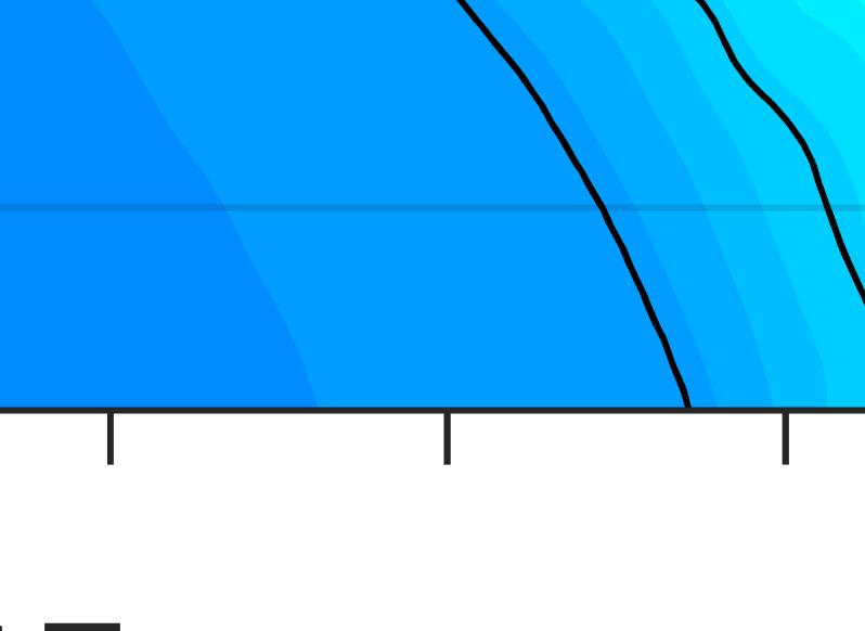
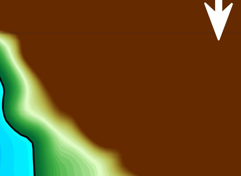
7 processes in (1), and the transport phenomena in (2), and 4) Evaluate the ability of rapidly evolving, state-of-the-art hydrostatic and non-hydrostatic circulation and wave models to simulate the key processes driving circulation, stratification and transport variability on the inner shelf. The Point Sal region located North of Point Conception CA was chosen as a field testing site for the activities of the DRI because of its strong wind driven circulation, eddy field, surface waves, and internal waves, and its diverse coastline and inner shelf topography (Fig. 1 and also See (Suanda et al. 2016)). Regional oceanographic background information can be found in studies by Washburn et al. (2011) and Aristizábal et al. (2016). The DRI has focused its efforts in many technical areas including in-situ observations, coastal and ship board radar, satellite and aircraft remote sensing, and numerical ocean modeling. In an effort to gain some insight into this lightly observed region (Cudaback and McPhee-Shaw 2009; Dever and Winant 2002) off the California coast, to test equipment, and to test a newly developed system of nested ocean models (Suanda et al. 2016), a pilot study was undertaken in the summer of 2015 termed the Point Sal Innershelf EXperiment (PSIEX) pilot. The whole suite of inner shelf DRI technical areas were at play during the pilot study, but of particular relevance to this study were in situ measurements of temperature and current made between the 50 and 20 m isobaths (Fig. 1, and Table 1) 1. Information concerning specific instrumentation on the moorings and sampling schemes is also presented in Table 1. The bottom topography is relatively simple between the 50 and 30 m isobaths but inshore of this area the bottom becomes more rough and rocky. There is a rocky outcrop rising up to 15 m water depth in the neighborhood of the O30 and O20 moorings. In the experimental region, current and temperature variability is dominated by nonlinear internal wave activity, and Fig. 2 shows 1 In situ measurements were made all the way into the 8-m isobath, but the focus of this study is on deeper water. 7

8 FIG Table examples of 4 different types of observed wave packets. By far the most common waves are waves of depression bringing warm water down from the surface and these waves correspond to internal tide bores (a), undular bores (b), and ISWs (c). The internal tide bore and undular bore are quite similar except the undular bore has many high frequency ISWs near the front face of the bore. In several cases the ISWs are separated from the bore and appear in groups (Fig. 2, Panel (c), yearday 205 to 205.2). In rarer cases, particularly in shallower depths, a reverse undular bore (d) is observed in which the bore forms on the rear of the wave and solitary waves of elevation bring cold water up from depth (Vlasenko and Hutter 2002; Duda et al. 2011). One of the strongest observational limitations of the data set are the noisy ADCP currents. Because of memory and power limitations, the ADCPs in this study sampled at a frequency of 1/5 Hz (one ping per 5 seconds) leading to smaller ensembles and some contamination by aliased surface gravity wave processes such as wave groups, infra-gravity waves and/or aliasing by the sea-swell band. While this noisiness is not important for the bores (due to their long timescale) it severely limits the ISW analysis. In particular the often useful vertical velocities for examining ISW dynamics(richards et al. 2013) could not be used here. The temperature observations, on the other hand, show the waves beautifully (Fig. 2), and since the T/S relationship in this region is relatively simple (Fig. 3 and See (Dever and Winant 2002)) temperature is a good indicator of vertical displacement. Because a consistent analysis procedure is sought for both bores and ISWs it is most practical to carry out the analysis using temperature alone. But current information is needed to derive energy fluxes and thereby examine dissipation processes. Through trial and error it has been determined that it is more insightful and accurate to derive current information from a displacement model using some approximations and kinematical constraints, than to work directly with the noisy current data. One exception to this rule is that the observed currents were used to 8

9 133 validate and slightly correct the kinematic results for the bore horizontal velocities (See Sec. 4). FIG Lastly the mooring array provides critical information about the large-scale environment in which the internal waves are propagating. Examples of low-pass filtered temporal variations in background stratification and current fields are shown in Figs. 4 and 5. The cut off frequency for all low-pass filtered data in this study is 0.25 cpd. A key result of this study is that stratification changes are an important factor affecting the statistics of the internal waves. The stratification changes are driven by winds (Lentz and Fewings 2012; Suanda et al. 2016) and by an active shelf eddy field 140 (Bassin et al. 2005). FIG. 4 FIG Wave Analysis The objectives of this section are two fold. First methods for wave detection and characterization are described. This step involves two idealized but quite effective models with a few simple parameters for match filtering in the time domain. The time domain approach is useful due to the transient wave nature of the bores and ISWs as well as the strong variability from wave to wave. Time domain techniques described here nicely complement harmonic methods which have had broad use (Nash et al. 2005). The second more challenging goal is that of taking the models with their fit parameters and inferring other properties of the waves such as speed, direction, energy flux and propagation loss. This second step involves several reasonable assumptions that will be discussed below and as such the derived wave quantities presented here should be considered to be a zero or first order approximation to reality. Estimated uncertainties are at the 10% level. The following sections provide an exposition of the adopted bore and ISW models and parameters as well as details of the match filtering and parameter estimation problem. 9

10 a. Bore Model A remarkably simple model represents the vast number of observed bores. Consider a mode 1, triangular waveform propagating in the x direction given by ζ(x, z, t) = ζ 0 ψ(z)(1 + (x x 0) c(t t 0 ) ), 0 < (x x 0 ) c(t t 0 ) <. (1) Here the wave packet group speed is c, the on-set time of the bore is t 0, and is the bore spatial width that can be related to the observed temporal width by = c t, (2) assuming a wave of fixed form. The bore mode function is ψ(z) and is computed using the linear, flat bottom, internal wave mode equation with rotation at the semi-diurnal frequency (Phillips 1977). Low-pass filtered temperatures are used to estimate buoyancy frequencies which are then used to compute the changing mode shapes over the course of the experiment (Fig. 4). The effects of background currents on the mode shapes are ignored. The mode is also given a unit normalization at the maximum value so that ζ 0 is the displacement amplitude. Empirical Orthogonal Function (EOF) analysis of the temperature and current records (not shown) supports the idea of a dominant mode 1 vertical structure as is commonly observed (Helfrich and Melville 2006; Apel et al. 2007). The objective is to fit this model locally to the moored observations by finding appropriate values of ζ 0, t 0 and t. The details of the fitting procedure are described in Sec. 3c. The fit parameters are thus a function of both time and mooring position. The issue of estimating the bore speed, c as well as its direction has some complications. The approach here is to take bore onset times 10

11 at multiple moorings and use plane wave beamforming to estimate speed and direction. These results are presented in Section 4.a, and the analysis reveals that the bores are primarily propagating perpendicular to the isobaths and that their speed is given to a reasonable approximation by the linear group speed, c 0, plus a first order KdV correction. The relation is c = c 0 + αζ 0 3, with α = 3c 0 0 D (ψ ) 3 dz 2 0 D (ψ ) 2 dz (3) where D is water depth, ψ is the derivative of ψ, and α is the nonlinear parameter from the standard KdV equation (Grimshaw et al. 2004; Apel et al. 2007) Having fit the displacement model to the observations a practical way forward is to use kinematics to estimate the currents. Here again the assumption is that background currents are not important but this is a complexity that may be relevant and will require further analysis (Grimshaw et al. 2004; Helfrich and Melville 2006). Ignoring advection, the vertical velocity is simply the time derivative of the displacement and the horizontal velocity in the direction of the wave is obtained via continuity ( u/ x = w/ z) yielding w(x, z, t) = ζ 0cψ u(x, z, t) = ζ 0 cψ [1 + (x x 0) c(t t 0 ) ]. (5) (4) Equation 5 slightly over estimates the observed u currents from the ADCPs where a factor of 0.8 is needed to bring them into agreement (See Sec 4.c). Given this encouraging result it is tempting to use the y component of the momentum equation ( v/ t = fu, the Coriolis parameter is f) to obtain the transverse current. This has been done but this model vastly over estimates the currents. 11

12 Furthermore the depth and temporal structure of the observed transverse currents is much more complicated than the in-plane currents, a result that was reported by Lerczak et al. (2003). In the foregoing analysis the transverse currents are therefore treated empirically based upon the ADCP observations. This is discussed further in Sec. 4. In addition, there are of course issues with discontinuities on the edges of this triangle wave but these effects will be ignored as second order. Here also the x dependence has been retained but when these results are applied to a single mooring this dependence is eliminated. In this case the maximum t t 0 = t The notation and approach of Moum et al. (2007b,a) are by-and-large followed in defining the wave energy quantities. Because transient wave events are being analyzed, the most fundamental quantity is the wave energy transmitted per length of coastline, E (J/m). This quantity is the vertically and horizontally integrated energy density, that is E = 0 D dz E dx = 0 D dz E cdt, (6) where the last step follows for a wave of fixed form. Here D is water depth and E is the wave energy density, kinetic plus potential in the linear limit given by E = ρ 2 (N 2 ζ 2 + w 2 + γu 2 ). (7) In Eq.7, γ is an O(1) empirical factor derived from the ADCP observations that accounts for a slight overestimate of u by the kinematic model and for the v contribution (See Sec. 4c, where we find γ = 0.82 utilizing v = uf/σ M2 ). If an idealized sinusoidal mode shape with vertical wave number 12

13 201 π/d is used, the triangular bore model has a simple form for E, namely E = ρ 0 2 ζ2 0c 2 [ N 2 D + D 3c γπ2 ], (8) 3D where N 2 is a water column average value of the squared buoyancy frequency. Here the order of the terms correspond to potential energy, vertical kinetic energy, and horizontal kinetic energy. In practice the integral over depth is done numerically with time dependent modes ψ(z) computed using a time dependent buoyancy frequency profile. Equation 8 is useful for showing the dependence on parameters, but it is not used directly in the analysis of the data. Because >> D for the bores one can safely ignore the vertical kinetic energy contribution in this expression. This is not necessarily so for the ISWs. 209 A transient energy flux (W/m) can be associated with the bore as follows f E = E t. (9) 210 A second form of energy flux is useful for this analysis and that is a daily average flux given by f E = 1 T J j=1 E j. (10) Here the energy of all the bores detected in a day (J) is summed up and then divided by the number of seconds in a day (T = 86, 400 s). This second form of energy flux will be useful when examining wave propagation loss. 13

14 b. ISW Model Now considering the ISWs, there is a similarly simple and useful model that has the same parameters as the bore model. Here a mode 1 Gaussian waveform is used given by ζ(x, z, t) = ζ 0 ψ(z) exp[ 4((x x 0) c(t t 0 )) 2 2 ]. (11) As with the bores, EOF analysis reveals the expected dominant mode 1 structure for the ISWs (Helfrich and Melville 2006; Apel et al. 2007). This Gaussian model is virtually identical to the classic hyperbolic secant squared ISW solution of the KdV equation, but it should be noted that in the present notation is the full width not the common half width of the ISW. The Gaussian form is used instead of the hyperbolic secant due to its relative analytic simplicity for the quantities of interest here. Here the ISW mode function, ψ(z), is computed using the linear, flat bottom, non-rotating mode equation at a frequency that is one quarter of the maximum buoyancy frequency. This choice of frequency means that rotation is not important and it yields mode shapes with either no turning points or with turning points close to the boundaries. This vertical structure is consistent with the observations as these mode shapes are fit to estimates of displacement as a function of depth (Sec. 2.c). As with the bore model the fit parameters, ζ 0, t 0 and t are all functions of both time and mooring position. The vertical and horizontal currents of the ISWs are obtained as described 14

15 228 previously for the bore model giving w(x, z, t) = 4ζ 0cψ(z) exp[ 4((x x 0) c(t t 0 )) 2 ][ 2((x x 0) c(t t 0 )) ] (12) 2 u(x, z, t) = ζ 0 cψ (z) exp[ 4((x x 0) c(t t 0 )) 2 v(x, z, t) 0. 2 ] (13) (14) The out of plane current, v, is taken to be zero because rotation has a small effect on these high frequency, small scale ISWs. As before with a mode vertical wave number of π/d, the wave energy per length of coastline has a simple analytic form namely E = ρ π 2 8 ζ2 0c 2 [ N 2 D + 2D 2c 2 + π2 ]. (15) 2D Here the first, second and third terms correspond to potential energy, vertical kinetic energy, and horizontal kinetic energy, and in practice the depth integral over the mode is done numerically using the time dependent mode shapes computed as described above The transient wave energy flux and the daily average flux for the ISWs are of the same form as that for the bores, namely Eqs. 9 and 10. This daily average flux is particularly important for quantifying the ISW propagation loss because it is rarely possible to track a specific wave across the moorings. Differences in daily average flux across shelf moorings then give a bulk measure of the wave losses. 15

16 c. Signal Processing FIG Because of the similarity of the bore and ISW models, the processing steps are nearly identical and therefore the exposition will be done together. The first step is the wave detection problem which includes the estimation of the wave time t 0, the wave time width t, and the wave temperature amplitude, T. Because temperature records are examined, the waves are most pronounced in the main thermocline. The wave detection analysis, therefore is carried out for the second and third sensor depths (Table 1), where the temperature records are band-pass filtered between 0.25 cpd and 24 cpd for the bore problem and the records are high pass filtered with a cut-off frequency of 24 cpd for the ISWs. The match filter is applied to the data as follows. At a given time ˆt 0 a Gauss-Markov estimation (Munk et al. 1995) (weighted least squares with priors) is carried out on a small time span of data around ˆt 0 to give a wave temperature amplitude T, a temperature offset, and a wave time width t. The data time span for bore/isw fits are t and 2 t. The fit yields a normalized mean square model-data mismatch of χ 2 (ˆt 0 ). This procedure is repeated at the next time step (30 seconds later) building up a timeseries of χ 2 (ˆt 0 ), T (ˆt 0 ), and t (ˆt 0 ). The wave detection is then carried out by examining χ 2 (ˆt 0 ) and finding minima in which the model accounts for over 50 percent of the data variance and where the temperature amplitude is positive (waves of depression). The minima then give wave times t 0 as well as T (t 0 ) and t (t 0 ). This procedure is applied at the two sensor depths in the main thermocline as sometimes for various reasons a detection is made at one depth but not the other. Examples of bore and ISW fits are shown in Fig. 6, and examples of waves and detections in the across shore and along shore directions are shown in Figs. 7 and Once the wave times and time widths are established then the Gauss-Markov fit is done over 16

17 all 5 sensors yielding a temperature amplitude as a function of depth, T (t 0, z). Using low-pass filtered temperature records, T lp (t, z), where the cut-off frequency is 0.25 cpd, the temperature amplitudes are converted to vertical displacement, ζ(t 0, z) using a nonlinear vertical interpolation method 2. The last step is to estimate the mode 1 amplitude, ζ 0 (t 0 ). This is done by computing the bore and ISW mode shapes from the low-pass filtered buoyancy frequency profiles (for example Fig. 4) as described above and then carrying out a least square fit to get ζ 0 (t 0 ). The depth fits are quite good by virtue of the dominant mode 1 EOF structure of the waves (See discussion on limitations below). Other quantities are also computed with the modes. The group speed, c 0 (t 0 ) and the KdV nonlinear parameter α(t 0 ) give an estimate of the wave speed, c(t 0 ) via Eq. 3, and depth integrals of ψ 2, N 2 ψ 2 and (ψ ) 2 are used for the depth integrated energy flux. A few words about the issues in carrying out this detection problem are necessary. The two conjoined main issues are data model mismatch and detection probability vs false alarm. With regards to data-model mismatch, Tables 2 and 3 show χ 2 statistics and the simple match filter models match 75-85% of the variability. It is important to point out that not all of the data/model misfit is about shortcomings of the model. Some of the misfit is variability that is associated with other processes that could not be filtered out. As for detection probability and false alarms, given certain threshold choices in the detector one must accept some number of missed detections and some number of false alarms. Via visual inspection we have chosen thresholds that capture nearly all the obvious wave events but do let in a few dubious waves. There are also rare cases when the model data mismatch is simply too severe to get a useful detection. The issue is not with the vertical structure of the waves which is quite robust but with the temporal structure. For the bores three main 2 The method goes as follows. The perturbed temperature at sensor z is given by T p (z) = T lp (z) + T (z). Using spline interpolation we then find the depth, ẑ, in the unperturbed profile where T lp (ẑ) = T p (z). The condition 0 ẑ D is enforced. The displacement is therefore ζ(z) = z ẑ. This nonlinear method is more accurate than the linear method of using the local temperature gradient. 17

18 FIG FIG. 8 situations arise. The first is when there is an undular bore, which when lowpass filtered, gives a bore on-set that is not as steep as a pure bore (Fig. 2). The second case is where the bore relaxation is not a simple linear decrease. This occurs for flat-top looking bores or when a bore splits into two bores perhaps due to nonlinear effects or wave interference. The third and last anomalous case is that of the reverse undular bore (Fig. 2). Similarly for the ISW s there are non-canonical looking waves, which include square or flat-topped ISW s perhaps due to strong non-linearity or a surface mixed layer, closely spaced or interfering ISWs, noisy ISWs perhaps due to mixing processes, and strongly surface intensified ISWs. As is evidenced by Figs. 7 and 8, the methods employed here are capturing most of the variability, though it is clear from the previous discussion that we cannot precisely close the error budgets with the present data set. 4. Statistics of Bores Table 2952 Bore statistics are addressed first as the ISWs are in fact spawned from the bores. Summary statistical information can be found in Table 2 for several observables. Because the bores are generally identifiable from mooring to mooring the question of speed and direction of propagation can be directly addressed: This is not the case for the ISWs. a. Speed and Direction To estimate bore speed and propagation direction, plane wave beamforming was carried out using the bore arrival times, t 0 at four different moorings, two each on the 50 and 30 m isobaths. The plane wave beamforming is implemented using the Gauss Markov method in this case to estimate the two parameters from the four arrival times at the moorings. Because of nonlinearities 18

19 the approach is to linearize the problem and iterate a few times to get convergence. The initial guess is c = 25 cm/s and propagation direction due East. The inversion is for the wave speed at the 50-m isobath and it is assumed that the speed has a D dependence. For the inversions both data error covariance and prior covariances are assumed diagonal, and specific values are 1 hr 2 for the variance of t 0, 100 (cm/s) 2 for the variance of c, and 400 deg 2 for the variance in the direction. A solution is considered acceptable if the data model residuals are all less than 1 hr which is the time scale of the low-pass filter used in the bore detection. An example using moorings S50, S30, LR50, and LR30 is provided in Fig. 9. Similar results are obtained for other groups of moorings but this case is particularly insightful because of the relative uniformity of the bottom slope along shelf. Here the observed wave speeds in Fig. 9 have been corrected for large scale background currents. Low-pass filtered barotropic currents (e.g. See Fig. 5) from the ADCPs at S50, S30, LR50, and LR30 were projected in the direction of wave propagation, averaged and then subtracted from the estimated speed described above. This procedure, with corrections ranging from -5 to +8 cm/s, significantly reduces the scatter in the estimated wave speeds thus giving confidence in the result. While there is some variability, the KdV corrected wave speeds computed using Eq. 3 show a close correspondence to the observed speeds (Fig. 9). The wave speeds are also responding to the changing stratification as exemplified by Fig. 4. For example there is a general speeding up of the waves as the summer stratification strengthens. This result provides confidence in the use of Eq. 3 for the calculation of energy fluxes. Note that time gaps in Fig. 9 occur where there are not 4 detections on each of the moorings or where there is large uncertainty in the bore time t 0. Note the gaps around yeardays 176 and 210 are due to a strong drop in bore energy (See Sec. 4.c). Lastly, the direction of bore propagation is slighly to the East-NorthEast (12 from East) with 19

20 323 FIG an rms of 10. Because of this result, it will be assumed in the subsequent analysis that the waves are propagating perpendicular to the local isobaths. b. Amplitude, Width, Separation, and Waves per Day The mode 1 displacement amplitude, ζ 0, the wave time width, t, the wave separation, t 0, and the number of waves per day, N w have been characterized. Summary statistics are shown in Table 2. The displacement amplitudes, ζ 0, are relatively large ranging from 1/5 to 1/2 the water depth thus attesting to the energy and nonlinearity of these waves. The average bore time widths, t, are close to 9 hours and are thus shorter than the semi-diurnal tidal period again attesting to the nonlinearity of the waves, and perhaps shoaling effects. While the bores themselves are shortened relative to the tidal period, the interval between bores, t 0 is still close to the tidal period which is an indicator of the regularity of the wave generation A key consideration is the along- and across-shelf variability. Along the 50-m and 30-m isobaths the statistics of ζ 0 and t are relatively homogenous. The greatest inhomogeneity is in the displacement statistics on the 30-m isobath where N30 is lower than the other three. This is due in part to the fact that the distance between N50 and N30 is roughly 0.90 km longer than the distances between the other lines (Table 1) In the across-shelf direction the O-line (O50, O40, O30, and O20) is of primary interest. Here the mean displacements show a steady decrease as the waves move onshore with a particularly large drop from O30 to O20 where the bores are propagating over the rough rocky outcrop (Fig. 1). Regarding time width the trend is toward widening bores as the waves propagate onshore. This suggests that dispersion is having an increasing effect on the bores as they weaken towards shore. 20

21 There is also the matter of number of bores per day, N w and the bore separation, which are shown in Table 2, columns 4 and 6. Here on average there are two bores per day, and roughly on every other day there is a third bore. Also the average bore separation is between 11 and 12 hours with an rms of 3 to 5 hours (Table 2, column 6). The variability in the bore arrival times, likely caused primarily by fluctuations in wave speed, can be associated with phase modulation of the internal tide leading to a loss of coherence with the local tide. Colosi and Munk (2006) show that the coherent and incoherent energy fractions are given by ν 2 and 1 ν 2 respectively where ν 2 = e θ2 and θ 2 is the mean square phase. The observations suggest θ 2 4 rad 2 thus giving a largely incoherent field (ν 2 = ). c. Energy Flux A key objective of the field work is to quantify internal wave energy fluxes and to come to an understanding of the processes that are responsible for their variation. Candidate processes have been discussed in Sec. 2. Before this is addressed, however, the matter of the bore transverse currents needs to be confronted. A comparison between observed bore horizontal currents by the ADCPs and modeled bore currents are shown in Fig. 10. Here the model is Eq. 5 and the y component of the linear momentum equation gives v, v(x, z, t) = ζ 0 fψ 2 [1 + (x x 2 0) c(t t 0 ) ]. (16) In spite of bandpass filtering around the semi-diurnal tide frequency the ADCP currents are quite noisy and so the important point here is not the scatter in Fig. 10 but the slopes. In the direction 21

22 FIG FIG of the wave, u, the observed and model currents are similar differing on average by a factor of 0.76 ± 0.02 (Fig. 10 ). At the 30-m isobath the factor is 0.81 ± The transverse currents, v, on the other hand, are dramatically over estimated by the model (Eq. 16), making this approach for estimating the bore energy flux untenable. However, the observed ratio of u to v in the bore is roughly what would be expected from a linear internal tide, that is the ratio f/σ M2 (Fig. 10 right panels). A semi-empirical approach is therefore taken in computing the energy flux contributions from the two components of the horizontal kinetic energy density, that is the u component of the horizontal kinetic energy density is computed using the model and then it is multiplied by the factor γ = (0.78) 2 (1 + (f/σ M2 ) 2 ) 0.82 to give the total horizontal kinetic energy. The mean and rms fluctuation of the bore energy density, E, the individual wave transient energy flux, f E, and the daily average energy flux f E are shown in Table 2. It is noteworthy that the rms values are of the same order of magnitude as the mean values which will have some implications for the physical interpretation of the variability in terms of interference. The temporal evolution of the daily averaged energy fluxes f E averaged along the 50 and 30 m isobaths are shown in Fig. 11. Variability over many timescales is observed. There is no apparent correlation to the spring neap cycle where spring/neap tides are expected near yeardays 166/175, 184/190, 196/205, and 213/220 (See Fig 1). The lack of spring/neap modulation is perhaps due to the 70 to 90 km propagation distance from the suspected generation region on Santa Rosa-Cortes Ridge to the innershelf. Over this long distance propagation and dissipation mechanisms could be masking the tidal modulation. Another possibility is that the internal tide is not generated locally but remotely (Nash et al. 2012). There are also no correlations with the background currents (Fig. 5). There are however two events of strongly diminished fluxes between yeardays and 22

23 that are associated with two periods of strongly reduced deep stratification (Figs. 11 and 4). The reduced fluxes are apparent in both the 50 and 30 m isobath records, but they are more clearly observed at the 50 meter site. Recall that this result is observed along a 10-km along shelf distance and so it is a large scale feature of the internal-wave field. The result could be due, in part, to neap tides that occurred on year days 175 and 205 which immediately preceded the drop in fluxes, but no similar drop in flux is observed during other neap tides. Another mechanism possibly explaining the loss is the transfer of energy from the bores to the solitons. These two periods do in fact correspond to times of increased soliton activity however the magnitude of the soliton fluxes are not large enough to account for all of the drop in bore flux (See Section 5). Also there are other times where the soliton activity is increased yet there is no corresponding drop in bore fluxes. Another possibility is another form of dissipation, perhaps due to mixing or instability Two more promising possibilities are as follows. First there could be seaward/shoreward shifts in the generation region thus increasing/decreasing the distance over which propagation loss can act. Another interesting possibility is a change in wave amplification due to subcritical bottom reflection, an effect that is sensitive to bottom stratification. The closer the bottom slope is to critical the more forward reflecting amplification occurs. Using ray theory the wave intensity amplification at frequency σ for one bottom bounce is sin(α + β) sin(α β), (17) where the subcritical group-propagation angle is α = tan 1 (σ 2 f 2 )/(N 2 σ 2 ) and the uniform bottom slope is β. Bottom slopes on the Point Sal inner and mid-shelf are in fact just below critical and fall in the range 0.4 to 0.5. For bottom stratification variation from 6 to 3 cph, α changes 23

24 from 0.62 to 1.23 giving a variation in the amplification factor of 2-9. If there are multiple bottom bounces involved the effects are multiplied. This is close to the factors needed to reconcile the low frequency variations in bore flux shown in Fig. 11. There is bore variability due to changes in the wave propagation environment but several factors point to another critical factor and that is interference. In Table 2 the rms values of energy densities and fluxes are comparable to the mean values. This is indicative of scintillation or strong interference phenomena typical in many branches of wave propagation especially optics and acoustics (Colosi 2016). In these cases the probability density function (PDF) is telling (Fig. 12). The bore PDF of energy flux resembles an exponential distribution. The physical interpretation of the exponential PDF comes from the central limit theorem (CLT) where if we consider the field to be a sum (interference) of many waves then the real and imaginary parts of the demodulated field tend towards zero mean Gaussian random variables as the number of waves tends towards infinite(colosi and Baggeroer 2004). The PDF of intensity is then a degree 2 chi-square distribution or exponential, and the PDF of wave amplitude is Rayleigh(Colosi 2016). The ratio of rms to mean for the Rayleigh and exponential distributions are 0.52 and 1.0 respectively. These values are consistent with the moments of displacement amplitude, ζ 0, and energy observables in Table 2. The energy flux PDF for the ISWs is also reminiscent of an exponential (Section 5). Pinning down the source of the interference in the bores will require further measurements but a little speculation is warranted. First, it is possible that the interference is coming from multiple sources of internal tide or horizontal plane propagation effects (Duda et al. 2014). Another possibility is that the bore statistics are being influenced by the ISWs because the majority of the bore events were undular bores that we attempt to smooth out with low pass filters (Fig. 2). In conclusion it is important to emphasize that the point of this PDF analysis is to show that the 24

25 observations have characteristics of interfering waves such as represented by the asymptotically valid exponential PDF. Our objective is not to do a hypothesis test, though this has been done. The Chi-square and Kolmogorov-Smirnov tests (Press et al. 1992) soundly reject the exponential PDF, 429 as is likely evident from the curves in Fig. 12. FIG. 12 d. Propagation Loss FIG All measures of bore energy or flux are observed to decay as the bores propagate onshore (Table 2), and the objective here is to quantify and characterize this propagation loss. Because the bores are propagating primarily perpendicular to the isobaths (Fig. 8), the wave propagation loss is defined as a gradient of the daily average energy fluxes between the 50 and 30 m isobaths, that is L E = f E(50) f E (30). (18) dx The distances dx as a function of mooring pairs (N50/N30, O50/O30, etc) are given in Table 1. A nearly linear relationship is obtained when the average flux between the 50 and 30 m isobaths, f 50,30 = (f E (50) + f E (30))/2 is plotted against the loss, L E (Fig. 13). This means that f E is expected to decay exponentially with distance towards shore where a linear fit to the data yields an e-folding scale of roughly x E = 2.4 ± 0.1 km. The exponential model also nicely represents the changes in mean fluxes along the O-line from the 50 to 20 m isobaths (Fig. 13 right panel). The decay rate is reasonable given that it is an average over all the 50 and 30 m isobath moorings The result that propagation loss is proportional to energy flux is not entirely unexpected since higher amplitude waves are more prone to instability. The relation between propagation loss and 25

26 FIG stratification is also of interest (Fig. 14). Here there is a slight tendency for the largest loss events to be associated with larger N but otherwise the loss is mostly independent of N. Unfortunately the field effort here did not have observations of turbulence and mixing, so the matter of bore dissipation cannot be properly addressed. Subsequent field efforts in the main experiment will rectify this situation. e. Dissipation Rate The exponential decay of the energy fluxes can also be interpreted in terms of a dissipation rate. Considering a 1-D balance, the wave energy equation is written E τ + ce x = 0, (19) where c is the group speed. Here it is important to distinguish between slow dissipation time τ and fast transient wave time t. This scale separation is a bit flimsy for the bores but is much better obeyed for the ISWs. Integrating Eq. 19 in both depth and time t an equation is obtained for the transient wave radiated energy density, E that is E τ + c E x = 0. (20) Because of the way transient wave energy flux was defined (Eqs. 9 and 10) this means E will also decay exponentially with propagation distance, and therefore the dissipation rate following the 456 wave is given by E τ = E (0) τ d exp[ τ τ d ]. (21) 26

27 Here τ d = x E /c is the dissipation timescale. At the 50-m isobath an average bore will have a transmitted wave energy density E of about 2.3 MJ per meter of coastline, and τ d 4.4 hours. The initial dissipation rate is then about 144 W per meter of coastline, lessening as the wave moves into shallower water. This large dissipation is a compelling observation in which the dissipated wave energy could be going to turbulence or since we are seeing a gradient in the momentum flux in the direction of the wave there could be a body force driving along shore flows via geostrophy (Winters 2015). These are questions for future study. 5. Statistics of Internal Solitary Waves The analysis of the ISWs is carried out along the same lines as that for the bores and of course there is a dynamical connection here since the bores are the source of the ISWs. A summary of 466 several ISW statistical quantities is shown in Table 3. Table 3 a. Speed and Direction Observationally establishing the speed and direction of the ISWs is problematic given the variability of the waves and the array geometry. The plane wave beamforming carried out on the bore arrivals cannot be done here because very rarely can an identifiable ISW be detected on two, let alone four moorings in our array. Since the bores are spawning the ISWs its not an unreasonable assumption that the ISWs are propagating in the same direction and roughly at the same speed as the bores. This has been confirmed by a small number of identifiable ISWs. With regards to ISW speed, there is some confidence in the KdV method (Eq. 3) which accurately re-produces the observed bore speeds (Fig. 9). Therefore in the following analysis it is assumed that the waves are 27

28 propagating perpendicular to the isobaths and that KdV theory is sufficient to estimate the wave speeds. Calculations of the ISW speeds over the duration of the experiment shows a similar time varying pattern to what was observed for the bores ( Fig. 9) except the ISW speeds are slightly faster (Table 3). This last fact is supported by images of the undular bores (Figs. 2 and 7 ) which shows the common occurrence of ISWs stretched out in front of the bores. b. Amplitude, Width, Separation, and Waves per day Four important ISW quantities that have been characterized are the ISW amplitude, the time width, the time separation between successive waves, and the number of waves per day. ISW displacement amplitudes are roughly one-third of those observed for the bores, but like the bores the displacements have large variability with rms fluctuations of order half the mean (typical of the Rayleigh distribution). The time widths also show a great deal of variability. In simple KDV theory there is a relationship between displacement and width such that larger waves are narrower until a maximal wave amplitude is reached after which the wave widens as the energy grows (Grimshaw et al. 2004; Apel et al. 2007). However, in this analysis a not so simple relationship is found: small narrow waves are just as likely to be found as large wide waves. The waves are also observed to be relatively close to one another. The average wave separation is roughly 3 wave widths and there is large variation about the mean. These three points: The large rms displacement relative to the mean, the lack of a relationship between displacement and width, and the close proximity of the waves to each other suggests that a nonlinear ISW interference pattern is being observed As with the bores a key consideration is the along- and across-shelf variability. Along the 50 and 30 m isobaths both displacement, time width, and time separation show relatively homogeneous 28

29 statistics (Table 3) which will allow for combining observations along isobaths to reduce sampling errors. In the across shelf direction there is clear inhomogeneity. Vertical displacements are observed to decay towards shore and the ISWs are narrowing in time width and time separation. More will be said about the decay of the waves but the narrowing and changing time separation of the waves is a topic that will likely need further analysis and modeling The number of ISWs in a day, N w is another important observable, particularly with regards to the amount of energy the ISWs transport over time. Not only does the displacement drop as the waves move toward shore but also the number of ISW s per day declines (Table 3). From the 50 to 20 m isobaths the rate of ISWs is reduced by a little over one half. The time evolution of ISW rate is also of interest and is shown in Fig. 15. There is no correlation here with the spring/neap cycle but 505 there is correlation with the low frequency variations in shallow stratification as described below. FIG. 15 c. Energy Flux Mean and rms fluctuation of the ISW energy density, E, individual wave transient energy flux, f E, and daily average energy flux f E are shown in Table 3. As in the case of the bores it is noteworthy that the rms values are of the same order of magnitude as the mean values which suggests interference. The discussion of the variability of the ISW s however will start with an examination of the temporal variability The temporal variation of ISW daily mean flux (f E ) for the 50 and 30 m isobaths are shown in Fig. 16. This variation is compared to the low-frequency temporal changes of the maximum stratification (depth mean N could be used too, but maximum N is chosen because the correlation is a bit clearer). The timeseries show that peaks/valleys in the stratification are associated with 29

30 FIG FIG peaks/valleys of the energy flux. Also, the fluctuations in daily average energy flux are largely attributable to the fluctuations in the ISW rate (Fig. 15). To first order, N is the generation rate of ISW s from a bore, that is a new ISW is added to the undular bore every buoyancy period (Apel 2003). Variations in N are of order a factor of 2 while changes in ISW rate and energy flux are much larger suggesting that there is slightly more afoot here than simply effects from N. Daily average fluxes tell one story but these values are the average over many ISWs. The individual ISW statistics show more variability and in all cases the rms fluctuation exceeds the mean sometimes over a factor of 2. (Table 3). This is an indication of coherent interference yielding strong focusing 3. The PDF of f E (Fig. 17) can be compared to the exponential and modulated exponential distributions(colosi et al. 2001b). The physical interpretation of the modulated exponential is of random wave interference consistent with the exponential distribution but with some modulation of the mean dictated by the parameter b. In this case an adequate comparison is obtained with b = 0.45 which indicates that the mean is modulated by 45%. The notion that ISWs in the undular bore or in packets of their own are interacting or interfering with each other is not new (Henyey and Hoering 1997; Badiey et al. 2013, 2016). As previously noted the point of this analysis is not to do a hypothesis test on any particular PDF model. The models simply demonstrate how interference and modulation effects can be manifest in the PDFs. d. Propagation Loss 532 Next the issue of propagation loss is addressed. Like the bores, if L E is plotted against f 50,30 3 An example of this phenomena of strong focusing are the bright bands/webs of light that can be observed on the bottom of a swimming pool as light passes through the wavy surface. Purely random interference does not create this pattern(colosi 2016). 30

31 a linear relation is obtained (Fig. 18 left panel) but in this case the e-folding distance is slightly shorter yielding x E = 2.0 ± 0.1 km. The exponential drop in mean energy flux across the O-line demonstrates the effect (Fig. 18 right panel). The observation that more energetic waves have greater loss was also reported by MacKinnon and Gregg (2003) and Shroyer et al. (2010). The relationship between propagation loss and maximum N is shown in Fig. 14, and the result is similar to the bore case. Some of the highest loss events are associated with large N, but for the majority of 539 the cases there is no clear relationship between loss and stratification. FIG. 18 e. Dissipation Rate Dissipation rates for the ISWs are estimated using Eq. 21. Again thinking of the 50-m isobath as a reference point, an average ISW will have a transmitted wave energy density E of about 20 kj per meter of coastline, and τ d 3.7 hours. The initial dissipation rate is then about 1.5 W per meter of coastline, lessening as the wave moves into shallower water. This is less than the dissipation rate for the bores (144 W/m) because of the smaller energy density. These values are also much smaller than measurements made on the Oregon (14 W/m) and New Jersey (50 W/m) shelves (Moum et al. 2007a; Shroyer et al. 2010). In both these cases wave dissipation was shown to be roughly in balance with observations of turbulence dissipation. 6. Summary and Conclusions Using some simple models and dynamical constraints, an effective time-domain methodology has been developed to allow detection and characterization of over 1000 bore and 9000 ISW wave events on the inner continental shelf off Point Sal CA over a 50 day period. This time domain 31

32 approach is essential given the variable and transient nature of the waves. The spirit of the problem is captured in the following question: How do you characterize a 12-hour wave that is different every 12 hours? Be that as it may, with the large ensemble of observed waves, the statistical behavior of several nonlinear internal wave characteristics have been well quantified. Importantly statistical behavior implies certain dynamics and two key results in this regard are 1) the observation of near exponential PDFs for bore and ISW energy flux suggesting strong wave interference and 2) the observed linear relationship between wave flux and propagation loss giving an exponential decrease in fluxes and dissipation rates towards shore. A relevant point here is that there is no such thing as a typical wave, rather it is the distribution functions of the waves that are of fundamental significance. In this work an attempt was made to implicate certain dynamical processes driving the variability. Here key issues are associated with the degree to which stratification changes, background flow fields, and topographic effects initiated by processes such as up/downwelling, eddies, and the coastal general circulation are modulating the waves. Dynamical processes of interest such as wave instability and mixing, bottom reflection amplification, wave refraction and interference, nonlinear wave-wave interaction, and transfer of energy from bores to ISWs may be working in isolation or in concert. Understanding such processes is pre-requisite to making headway on other important questions such as quantifying the transport of heat, salt, momentum, and other quantities in the inner shelf, estimating novel stresses imposed on the large scale circulation by small scale processes, and even for understanding acoustic propagation. But, more questions are raised than are answered, and our data has limitations such that error budgets cannot be completely closed. Therefore new modeling and observational efforts will be required to come to a dynamical understanding of the observed wave distribution functions. 32

33 Acknowledgments: This work was supported by the Office of Naval Research, and is funded under the inner shelf DRI. The authors are appreciative of the able captain and crew of the R/V Oceanus for enabling the successful deployment and recovery of the instrumentation used in this work. Special thanks to Jim Moum, and Tim Duda for enlightening discussions and helpful comments on many versions of the paper. 33

34 REFERENCES Apel, J., M. Badiey, C. Chiu, S. Finnette, R. Headrick, J. Kemp, J. Lynch, A. Newhall, M. Orr, B. Pasewark, D. Teilbuerger, A. Turgut, K. von der Heydt, and S. Wolf, 1997: An overview of the 1995 swarm shallow water internal wave acoustic scattering experiment. IEEE J. Oceanic Eng., 22, Apel, J., L. Ostrovsky, Y. A. Stepanyants, and J. Lynch, 2007: Internal solitons in the ocean and their effect on underwater sound. J. Acoust. Soc. Am., 121(2), Apel, J. R., 2003: A new analytical model for internal solitons in the ocean. J. Phys. Oc., 33, Aristizábal, M. F., M. R. Fewings, and L. Washburn, 2016: Contrasting spatial patterns in the diurnal and semidiurnal temperature variability in the santa barbara channel, california. J. Geophys. Res. Oc., 121, Badiey, M., L. Wan, and J. Lynch, 2016: Statistics of nonlinear internal waves during the shallow water 2006 experiment. J. Atmos. Oc. Tech., 33, Badiey, M., L. Wan, and A. Song, 2013: Three-dimensional mapping of evolving internal waves during the shallow water 2006 experiment. JASA Exp. Lett., 134. Bassin, C., L. Washburn, M. Brzezinki, and E. McPhee-Shaw, 2005: Sub-mesoscale coastal eddies observed by high frequency radar: A new mechanism for delivering nutrients to kelp forests in the southern california bight. Geophys. Res. Let., 32, Brink, K. H., 1988: On the effect of bottom friction on internal waves. Cont. Shef Res., 8(4), Colosi, J., 2016: Sound Propagation through the Stochastic Ocean. Cambridge University Press, 420 pp. 34

35 Colosi, J., R. Beardsley, J. Lynch, G. Gawarkiewicz, C. Chiu, and A. Scotti, 2001a: Observations of nonlinear internal waves on the outer new england continental shelf during the summer shelfbreak primer study. J. Geophys. Res. Oceans, 106(C5), Colosi, J., F. Tappert, and M. Dzieciuch, 2001b: Further analysis of intensity fluctuations from a 3252-km acoustic propagation experiment in the eastern north pacific ocean. J. Acoust. Soc. Am., 110, Colosi, J. A., and A. B. Baggeroer, 2004: On the kinematics of broadband multipath scintillation and the approach to saturation. J. Acoust. Soc. Am., 116(6), Colosi, J. A., and W. Munk, 2006: Tales of the venerable honolulu tide gauge. J. Phys. Oc., 36, Cudaback, C. N., and E. McPhee-Shaw, 2009: Diurnal-period internal waves near point conception, california. Estuary, Coastal and Shelf Science, 83, Dever, E., and C. Winant, 2002: The evolution and depth structure of shelf and slope temperatures and velocities during the el nino near point conception, california. Progr. in Oc., 54, Duda, T., and D. Farmer, 1999: The 1998 whoi/ios/onr internal solitary wave workshop: Contributed papers. WOODS HOLE OCEANOGRAPHIC INSTITUTION Technical Report. Duda, T. F., Y. Lin, and B. Reeder, 2011: Observationally constrained modeling of sound in curved ocean internal waves: Examination of deep ducting and surface ducting at short range. J. Acoust. Soc. Am., 130, Duda, T. F., W. G. Zhang, K. R. Helfrich, A. E. Newhall, Y.-T. Lin, J. F. Lynch, P. Lermusiaux, P. Haley, and J. Wilkin, 2014: Issues and progress in the prediction of ocean submesoscale features and internal waves Oceans-St. John s, IEEE,

36 Eriksen, C., 1998: Internal wave reflection and mixing at fieberling guyot. J. Geophys. Res., 103, Grimshaw, R., E. Pelinovsky, T. Talipova, and A. Kurkin, 2004: Simulation of the transform of internal solitary waves on oceanic shelves. J. Phys. Oc., 34, Helfrich, K. R., and W. K. Melville, 2006: Long nonlinear internal waves. Annu. Rev. Fluid Mech., 38, Henyey, F. S., and A. Hoering, 1997: Energetics of borelike internal waves. J. Geophys. Res. Oc., 102, Lamb, K. G., 2014: Internal wave breaking and dissipation mechanisms on the continental slope/shelf. Ann. Rev. Fl. Mech., 46, Lee, C., and R. Beardsley, 1974: The generation of long nonlinear internal waves in a weakly stratified shear flow. J. Geophys. Res., 79(3), Lentz, S., and M. Fewings, 2012: The wind- and wave- generated inner-shelf circulation. Annu. Rev. Mar. Sci., 4, 317?343. Lerczak, J. A., C. Winant, and M. Hendershott, 2003: Observations of the semidiurnal internal tide on the southern california slope and shelf. Journal of Geophysical Research: Oceans, 108. Liu, A. K., 1988: Analysis of nonlinear internal waves in the new york bight. J. Geophys. Res. Oc., 93, MacKinnon, J., and M. Gregg, 2003: Mixing on the late-summer new england shelf-solibores, shear, and stratification. J. Phys. Oc., 33, Moum, J., D. Farmer, E. Shroyer, W. Smyth, and L. Armi, 2007a: Dissipative losses in nonlinear internal waves propagating across the continental shelf. J. Phys. Oc., 37, Moum, J., D. Farmer, W. Smyth, L. Armi, and S. Vagle, 2003: Structure and generation of turbulence 36

37 at interfaces strained by internal solitary waves propagating shoreward over the continental shelf. J. Phys. Oc., 33, Moum, J. N., J. M. Klymak, J. D. Nash, A. Perlin, and W. D. Smyth, 2007b: Energy transport by nonlinear internal waves. J. Phys. Oc., 37(7), Munk, W., P. Worcester, and C. Wunsch, 1995: Ocean Acoustic Tomography. Cambridge University Press, 433 pp. Nash, J., M. Alford, and E. Kunze, 2005: Estimating internal wave energy fluxes in the ocean. J. Atmos. and Oc. Tech., 22, Nash, J. D., S. M. Kelly, E. L. Shroyer, J. N. Moum, and T. F. Duda, 2012: The unpredictable nature of internal tides on continental shelves. J. Phys. Oc., 42, Phillips, O. M., 1977: The Dynamics of the Upper Ocean, 2 nd edition. Cambridge University Press, 336 pp. Press, W. H., S. A. Teukolsky, W. T. Vetterling, and B. P. Flannery, 1992: Numerical Recipes in FORTRAN, Second Edition. Cambridge University Press. Ramp, S. R., T. Y. Tang, T. F. Duda, J. F. Lynch, A. K. Liu, C.-S. Chiu, F. L. Bahr, H.-R. Kim, and Y.-J. Yang, 2004: Internal solitons in the northeastern south china sea. part i: Sources and deep water propagation. IEEE J. Oc. Eng., 29, Richards, C., D. Bourgault, P. S. Galbraith, A. Hay, and D. E. Kelley, 2013: Measurements of shoaling internal waves and turbulence in an estuary. J. Geophys. Res.: Oceans, 118, Scotti, A., R. Beardsley, and B. Butman, 2006: On the interpretation of energy and energy fluxes of nonlinear internal waves: An example from massachusetts bay. J. Fluid Mech., 561, Shroyer, E., J. Moum, and J. Nash, 2010: Energy transformations and dissipation of nonlinear internal waves over new jersey s continental shelf. Nonlinear processes in Geophysics, 17, 37

38 : Nonlinear internal waves over new jersey s continental shelf. J. Geophys. Res., 116(C3). Suanda, S. H., N. Kumar, A. J. Miller, E. Di Lorenzo, K. Haas, D. Cai, C. A. Edwards, L. Washburn, M. R. Fewings, R. Torres, and F. Feddersen, 2016: Wind relaxation and a coastal buoyant plume north of pt. conception, ca: Observations, simulations, and scalings. J. Geophys. Res.: Oceans, 121, Vlasenko, V., and K. Hutter, 2002: Numerical experiments on the breaking of solitary internal waves over a slope-shelf topography. J. Phys. Oc., 32, Walter, R. K., C. B. Woodson, P. R. Leary, and S. G. Monismith, 2014: Connecting wind-driven upwelling and offshore stratification to nearshore internal bores and oxygen variability. J. Geophys. Res. Oc., 119, Washburn, L., M. R. Fewings, C. Melton, and C. Gotschalk, 2011: The propagating response of coastal circulation due to wind relaxations along the central california coast. J. Geophys. Res. Oc., 116. Wheelon, A. D., 2003: Electromagnetic Scintillation, Vols 1-3. Cambridge University Press. Winters, K., 2015: Tidally-forced flow in a rotating, stratified, shoaling basin. Ocean Modelling, 90, Wunsch, C., and R. Hendry, 1972: Array measurements of the bottom boundary layer and the internal wave field on the continental slope. Geophys. Fluid Dyn., 4, Zhang, S., M. Alford, and J. Mickett, 2015: Characteristics, generation, and mass transport of nonlinear internal waves on the washington continental shelf. J. Geophys. Res. Oceans. Zhang, W. G., T. F. Duda, and I. A. Udovydchenkov, 2014: Modeling and analysis of internal-tide generation and beamlike onshore propagation in the vicinity of shelfbreak canyons. J. Phys. Oc., 38

39 694 44,

40 Generated with ametsocjmk.cls. Written by J. M. Klymak jklymak/worktools.html 40

41 Tables Mooring Mean Depths (Temperature) Distance to Neighbors Location (m) (km) (Lat,Long) S50 6.2,16.5,26.4, 36.3,46.2 LR50: 3.05, S30: , LR50 5.7,16.0,26.1,35.9,45.8 O50: 3.43, LR30: , O50 6.2,16.3,29.7,36.1,46.1 N50: 3.30, O40: , N50 5.2,15.5,25.8,35.4,45.3 O50: 3.30, N30: , O40 5.1,10.1,20.1,30.0,35.0 O50: 2.00, O30: , S30 5.3,10.5,15.5,20.4,25.4 LR30: 3.08, S50: , LR30 5.1,10.2,15.2,20.2,25.1 O30: 2.76, LR50: , O30 6.7,11.6,16.6,21.6,26.5 N30: 2.99, O40: , N30 4.9,10.2,15.1,20.1,25.0 O30: 2.99, N50: , O20 0.5,3,6,9,12,15,17,19 O30: , Table 1. Summary of moored temperature and current measurements for the PSIEX pilot. All moorings have complete records between 15 June and 6 August 2015 (yeardays ), except O20 whose record runs from 09 June to 23 July 2015 (yeardays ). On the 50, 40, and 30 meter moorings temperature measurements were made with SBE9 instruments (some with pressure) sampling every 30 seconds. On the 20 meter mooring temperature was measured using RBR instruments sampling at 1 Hz. Each location also had a nearby ADCP. The 300 khz RDI ADCPs at these locations sampled at 12 pulses per minute with 2 m bins, except for the O20 location which had a 1000 khz Nortek Aquadopp sampling at 1 Hz with 1-m bins. There were no pressure sensors on the O20 mooring so depths are nominal. 41

42 Events 1 χ 2 N w ζ 0 t 0 t c E f E f E (m) (hrs) (hrs) (cm/s) (MJ/m) (W/m) (W/m) S / /0.6 18/ / /2.7 18/ /2.0 68/46 55/38 LR / /0.6 18/ / /2.5 18/ /1.9 66/45 57/35 O / /0.6 17/ / /2.6 18/ /1.7 62/44 52/33 N / /0.5 18/ / /2.9 18/ /1.9 70/46 56/38 O / /0.6 14/ / /2.9 15/ / /22 27/19 S / /0.5 12/ / /2.6 12/ / /9.1 13/8.7 LR / /0.5 11/ / /2.8 12/ / /11 15/7.0 O / /0.6 12/ / /3.1 13/ / /12 15/9.3 N / /0.7 10/ / /3.2 13/ / /12 13/9.4 O / / / /4.8 10/ / / / /1.7 50m / /0.6 18/ / /2.7 18/ /1.9 67/45 55/36 30m / /0.6 11/4 11.7/ /3.0 13/ / /11 14/8.6 Table 2. Statistics of internal tide bores observed during the PSIEX pilot. In columns 3-11 the mean and root mean square (rms) fluctuation are shown in the format (mean/rms). The observables in columns 2-11 are, total number of bores detected, normalized rms temperature variability described by the bore model fit (1 is a perfect fit), number of bores per day, bore displacement amplitude, time separation between successive bores, bore time width, bore speed (Eq. 3), bore energy per length of coastline (Eq. 6), transient bore energy flux (Eq. 9), and daily average energy flux (Eq. 10). The last two rows are averages over the 50 and 30 m isobaths. We define t 0 as the time difference between successive bores. 42

43 Events 1 χ 2 N w ζ 0 t 0 t c E f E f E (m) (min) (min) (cm/s) (kj/m) (W/m) (W/m) S / /14 7.3/ /13 7.6/3.9 19/2.7 20/38 40/63 5.5/4.3 LR / /12 6.9/ /13 8.2/3.9 19/2.6 19/36 36/57 4.9/3.9 O / /14 7.3/ /13 8.2/3.8 19/2.4 22/42 40/64 5.2/5.0 N / /14 7.0/ /13 8.3/3.8 19/2.5 20/33 38/57 5.5/4.7 O / /14 5.7/ /13 7.6/3.9 15/ /13 17/24 1.6/1.6 S / /15 5.1/ /13 6.5/3.4 14/ /6.4 11/ /0.90 LR / /12 4.6/ /13 6.6/4.0 13/ / / /0.78 O / /10 5.1/ /13 6.8/3.8 13/ /6.5 10/ /0.72 N / /9 4.7/ /13 7.1/3.6 14/ / / /0.75 O / /9 2.1/ /12 5.6/ / / / / m / /15 7.1/ /13 8.1/3.8 19/2.6 20/37 39/61 5.3/4.5 30m / /12 4.7/ /13 6.7/3.7 14/ /6.4 10/ /0.80 Table 3. Statistics of internal solitary waves observed during the PSIEX pilot. In columns 3-11 the mean and root mean square (rms) fluctuation are shown in the format (mean/rms). The observables in columns 2-11 are, total number of ISWs detected, normalized rms temperature variability described by the ISW model fit (1 is a perfect fit), number of ISWs per day, ISW displacement amplitude, time separation between successive ISWs, ISW time width, ISW speed (Eq. 3), ISW energy per length of coastline (Eq. 6), transient ISW energy flux(eq. 9), and daily average energy flux (Eq. 10). The last two rows are averages over the 50 and 30 m isobaths. We define t 0 as the time difference between successive ISWs in a wave packet, therefore only time differences less than 1 hour are considered in the statistics. 43

44 Figure Captions FIG. 1. Experimental setting of the Point Sal region with mooring names and locations (red squares), and tide elevation at Port San Luis. Isobath contours start at 10 meters and increase in 5 meter increments to 55 meter. The most prominent topographic feature is the rocky outcrop between moorings O30 and O20. The across shelf transect, termed the O-line, is marked with a white line. For reference the distance between the S50 and N50 moorings is 9.8 km, the distance between S50 and S30 is 3.1 km, and the distance across the O-lines is 5.1 km. Between the 50 and 30 m isobaths the sea floor slope is slowly changing in the along shore direction and the slope has values roughly in the range 0.3 and 0.6 deg. FIG. 2. Examples of four different types of nonlinear internal wave packets observed during PSIEX: (a) bore alone, (b) undular bore, (c) internal solitary waves, and (d) reverse undular bore. The reverse undular bore is the least common wave by far and is most likely observed in the shallowest water. FIG. 3. Temperature and Salinity relationship for PSIEX (dots) derived from 10 CTD cats taken aboard the R/V Oceanus 6-10 August The continuous curve is a third order polynominal fit to the observations. FIG. 4. Buoyancy frequency variability observed at the LR50 mooring which is a typical pattern observed at the other moorings. Buoyancy frequency profiles were computed from the low-pass filtered temperature records using a thermal expansion coefficient of (1/ C) from the equation of state with S=33.44 PSU, T=14 C, and P=20 dbar. The thermal expansion coefficient translates the vertical temperature gradient into a potential density gradient. The cut off frequency is 0.25 cpd. FIG. 5. An example of low pass filtered barotropic (a) and baroclinic (b) and (c) currents observed on the LR50 mooring which is a typical pattern observed at the other moorings. The cut off frequency is 0.25 cpd. At this mooring the u and v components of the current are approximately in the across/along isobath directions. FIG. 6. Examples of bore (a) and ISW (b) fits for the O40 mooring. Observations are shown with solid lines and fits are shown with dash lines. 44

45 FIG. 7. Examples of bore and ISW detections on the O-line between the 50 and 20 m isobaths. Moorings O50, O40, O30, and O20 are depicted in panels (a), (b), (c), and (d). Green marks shows ISWs and red marks show bores. FIG. 8. Examples of bore and ISW detections along the 50 m isobath. Moorings N50, O50, LR50, and S50 are depicted in panels (a), (b), (c), and (d). Green marks shows ISWs and red marks show bores. FIG. 9. Planewave beamforming results for wave speed c (a) and direction (b) using bore arrival times, t 0 at the 4 moorings S50, S30, LR50, and LR30. The observed wave speeds are corrected for background currents using low pass filtered barotropic currents projected in the direction of propagation and estimated using ADCP data from the 4 mooring locations. Theoretical estimates of wave speed at S50 and LR50 using the linear bore group speed plus the KdV correction (Eq. 3) are shown with plusses. Mean and root mean square (rms) fluctuation of the wave speed and direction are 20 and 6 cm/s and 12 and 10 degrees. Similar results are obtained for other mooring combinations. FIG. 10. Comparisons between observed and estimated/modeled mode 1 maximum bore currents at the 50 meter isobath (a) and (b). Also shown is the distribution of observed maximum u and v currents indicating the level of the momentum balance in the model (c), where it should be noted f/σ M2 = The observed current is estimated from the ADCP data which is bandpass filtered between timescales of 3 and 20 hours. There is considerable scatter in the data giving R 2 values for the three panels of 0.45, 0.20, and Similar results are obtained at the 30-m isobath. FIG. 11. (a) Average buoyancy frequency at 45-m depth along the 50-m isobath, with labels for the Spring (S) and Neap (N) tides. Isobath averaged time series of bore daily average energy flux, f E, for the 50 m (b) and 30 m (c) isobaths. FIG. 12. Probability density function (PDF) of bore f E / f E averaged over the 50 and 30 m isobaths (Solid). The PDF is estimated from 846 observations of bore energy flux. For qualitative comparison purposes the exponential PDF indicative of wave interference is shown (dash). FIG. 13. (a) Average bore energy flux between the 50 and 30 m isobaths plotted against bore propagation loss L E. A straight line fit to the points yields a slope of 2.4±0.1 km (R 2 = 0.83). A few points where the loss is negative have been excluded from the fit. (b) Mean daily average energy fluxes along the O-line (Table 2) are plotted with the exponential decay (dash) expected from the straight line fit in (a). The exponential curve at distance zero has a value of 55 W/m which 45

46 is the mean value on the 50-m isobath (Table 2). Errorbars represent the error in the mean given 20 independent samples. FIG. 14. A scatter plots of bore (a) and ISW (b) propagation loss L E vs maximum buoyancy frequency during the event. In rare cases there is negative loss meaning an increase in wave energy. FIG. 15. Timeseries of number of ISW events observed per day on the 50 meter (a) and 30 meter (b) isobaths. The spring/neap cycle is identified by the symbols S and N. FIG. 16. Maximum buoyancy frequency of the isobath averaged buoyancy frequency profiles on the 50 meter (a) and 30 meter (b) isobaths. Average time series of ISW f E on the 50 meter (c) and 30 meter (d) isobaths. The spring/neap cycle is identified by the symbols S and N. FIG. 17. Probability density function (PDF) of ISW f E / f E averaged over the 50 and 30 m isobaths (Solid). The PDF is estimated from 7822 observations of energy flux. For qualitative comparison purposes two model PDFs are shown, the exponential (dash) and the modulated exponential with b = 0.45 (dash-dot). FIG. 18. (a) Average ISW energy flux between the 50 and 30 m isobaths plotted against ISW propagation loss L E. A straight line fit to the points yields a slope of 2.0±0.1 km (R 2 = 0.87). A few points where the loss is negative have been excluded from the fit. (b) Daily average energy fluxes along the O-line (Table 2) are plotted with the exponential decay (dash) expected from the straight line fit in (a). The exponential curve at distance zero has a value of 5.7 W/m which is the mean value on the 50-m isobath (Table 2). Errorbars represent the error in the mean given 20 independent samples. 46

47 Figures F IG. 1. Experimental setting of the Point Sal region with mooring names and locations (red squares), and tide elevation at Port San Luis. Isobath contours start at 10 meters and increase in 5 meter increments to 55 meter. The most prominent topographic feature is the rocky outcrop between moorings O30 and O20. The across shelf transect, termed the O-line, is marked with a white line. For reference the distance between the S50 and N50 moorings is 9.8 km, the distance between S50 and S30 is 3.1 km, and the distance across the O-lines is 5.1 km. Between the 50 and 30 m isobaths the sea floor slope is slowly changing in the along shore direction and the slope has values roughly in the range 0.3 and 0.6 deg. 47

48 FIG. 2. Examples of four different types of nonlinear internal wave packets observed during PSIEX: (a) bore alone, (b) undular bore, (c) internal solitary waves, and (d) reverse undular bore. The reverse undular bore is the least common wave by far and is most likely observed in the shallowest water. 48

49 FIG. 3. Temperature and Salinity relationship for PSIEX (dots) derived from 10 CTD cats taken aboard the R/V Oceanus 6-10 August The continuous curve is a third order polynominal fit to the observations. 49

50 FIG. 4. Buoyancy frequency variability observed at the LR50 mooring which is a typical pattern observed at the other moorings. Buoyancy frequency profiles were computed from the low-pass filtered temperature records using a thermal expansion coefficient of (1/ C) from the equation of state with S=33.44 PSU, T=14 C, and P=20 dbar. The thermal expansion coefficient translates the vertical temperature gradient into a potential density gradient. The cut off frequency is 0.25 cpd. 50

51 FIG. 5. An example of low pass filtered barotropic (a) and baroclinic (b) and (c) currents observed on the LR50 mooring which is a typical pattern observed at the other moorings. The cut off frequency is 0.25 cpd. At this mooring the u and v components of the current are approximately in the across/along isobath directions. 51

52 FIG. 6. Examples of bore (a) and ISW (b) fits for the O40 mooring. Observations are shown with solid lines and fits are shown with dash lines. 52

53 FIG. 7. Examples of bore and ISW detections on the O-line between the 50 and 20 m isobaths. Moorings O50, O40, O30, and O20 are depicted in panels (a), (b), (c), and (d). Green marks shows ISWs and red marks show bores. 53

54 FIG. 8. Examples of bore and ISW detections along the 50 m isobath. Moorings N50, O50, LR50, and S50 are depicted in panels (a), (b), (c), and (d). Green marks shows ISWs and red marks show bores. 54

55 FIG. 9. Planewave beamforming results for wave speed c (a) and direction (b) using bore arrival times, t 0 at the 4 moorings S50, S30, LR50, and LR30. The observed wave speeds are corrected for background currents using low pass filtered barotropic currents projected in the direction of propagation and estimated using ADCP data from the 4 mooring locations. Theoretical estimates of wave speed at S50 and LR50 using the linear bore group speed plus the KdV correction (Eq. 3) are shown with plusses. Mean and root mean square (rms) fluctuation of the wave speed and direction are 20 and 6 cm/s and 12 and 10 degrees. Similar results are obtained for other mooring combinations. 55

56 FIG. 10. Comparisons between observed and estimated/modeled mode 1 maximum bore currents at the 50 meter isobath (a) and (b). Also shown is the distribution of observed maximum u and v currents indicating the level of the momentum balance in the model (c), where it should be noted f/σ M2 = The observed current is estimated from the ADCP data which is bandpass filtered between timescales of 3 and 20 hours. There is considerable scatter in the data giving R 2 values for the three panels of 0.45, 0.20, and Similar results are obtained at the 30-m isobath. 56

57 FIG. 11. (a) Average buoyancy frequency at 45-m depth along the 50-m isobath, with labels for the Spring (S) and Neap (N) tides. Isobath averaged time series of bore daily average energy flux, f E, for the 50 m (b) and 30 m (c) isobaths. 57

58 FIG. 12. Probability density function (PDF) of bore f E / f E averaged over the 50 and 30 m isobaths (Solid). The PDF is estimated from 846 observations of bore energy flux. For qualitative comparison purposes the exponential PDF indicative of wave interference is shown (dash). 58

59 FIG. 13. (a) Average bore energy flux between the 50 and 30 m isobaths plotted against bore propagation loss L E. A straight line fit to the points yields a slope of 2.4±0.1 km (R 2 = 0.83). A few points where the loss is negative have been excluded from the fit. (b) Mean daily average energy fluxes along the O-line (Table 2) are plotted with the exponential decay (dash) expected from the straight line fit in (a). The exponential curve at distance zero has a value of 55 W/m which is the mean value on the 50-m isobath (Table 2). Errorbars represent the error in the mean given 20 independent samples. 59

60 FIG. 14. A scatter plots of bore (a) and ISW (b) propagation loss L E vs maximum buoyancy frequency during the event. In rare cases there is negative loss meaning an increase in wave energy. 60

61 FIG. 15. Timeseries of number of ISW events observed per day on the 50 meter (a) and 30 meter (b) isobaths. The spring/neap cycle is identified by the symbols S and N. 61