FFI RAPPORT SENSITIVITY OF LYBINS TRANSMISSION LOSS DUE TO VARIATIONS IN SOUND SPEED. HJELMERVIK Karl Thomas FFI/RAPPORT-2006/01356

Transcription

1 FFI RAPPORT SENSITIVITY OF LYBINS TRANSMISSION LOSS DUE TO VARIATIONS IN SOUND SPEED HJELMERVIK Karl Thomas FFI/RAPPORT-2006/01356

2

3 SENSITIVITY OF LYBINS TRANSMISSION LOSS DUE TO VARIATIONS IN SOUND SPEED HJELMERVIK Karl Thomas FFI/RAPPORT-2006/01356 FORSVARETS FORSKNINGSINSTITUTT Norwegian Defence Research Establishment P O Box 25, NO-2027 Kjeller, Norway

4

5 3 FORSVARETS FORSKNINGSINSTITUTT (FFI) Norwegian Defence Research Establishment UNCLASSIFIED P O BOX 25 SECURITY CLASSIFICATION OF THIS PAGE N KJELLER, NORWAY (when data entered) REPORT DOCUMENTATION PAGE 1) PUBL/REPORT NUMBER 2) SECURITY CLASSIFICATION 3) NUMBER OF FFI/RAPPORT-2006/01356 UNCLASSIFIED PAGES 1a) PROJECT REFERENCE 2a) DECLASSIFICATION/DOWNGRADING SCHEDULE 41 FFI-IV/899/914-4) TITLE SENSITIVITY OF LYBINS TRANSMISSION LOSS DUE TO VARIATIONS IN SOUND SPEED 5) NAMES OF AUTHOR(S) IN FULL (surname first) HJELMERVIK Karl Thomas 6) DISTRIBUTION STATEMENT Approved for public release. Distribution unlimited. (Offentlig tilgjengelig) 7) INDEXING TERMS IN ENGLISH: IN NORWEGIAN: a) Raytrace a) Strålegang b) Sound speed b) Lydhastighet c) Sensitivity-analysis c) Følsomhetsstudie d) Measurements d) Målinger e) Acoustic modelling e) Akustisk modellering THESAURUS REFERENCE: 8) ABSTRACT This study is motivated by the Sea Acceptance Test 2 (SAT2) to be made sometime in The testing of the new Norwegian Frigates sonar system will involve use of the acoustic ray trace model, LYBIN. The study reveals that LYBIN is sensitive to certain types of errors in the sound speed, depending on the depth of the sonar. The modelling of the hull-mounted Spherion sonar is sensitive to changes in the surface sound speed, while the variable-depth CAPTAS sonar is more sensitive to sound speed changes at and close to the sonar depth. Suggested procedures regarding monitoring of the sound speed and the depth of the variable-depth sonar during the SAT2-tests are made. 9) DATE AUTHORIZED BY POSITION This page only Elling Tveit Director of Research ISBN UNCLASSIFIED SECURITY CLASSIFICATION OF THIS PAGE (when data entered)

6

7 5 CONTENTS Page 1 EXCECUTIVE SUMMARY 7 2 INTRODUCTION 8 3 METHODS AND CONCEPTS Ray concepts Methods of comparison 9 4 ENVIRONMENTS Artificial sound speed profiles Constant gradient Surface channel Deep sound channel Measured sound speed profiles Poseidon sea trial, September 2005, CTD-line RESULTS Artificial sound speed profiles Constant gradient Surface channel Deep sound channel Measured sound speed profiles 23 6 CONCLUSION 27 APPENDIX A COMPARISON PLOTS, POSEIDON CTD-LINE 1 29 A.1 Source at 5m depth 29 A.2 Source at 50m depth 33 A.3 Source at 100m depth 37 References 41

8 6

9 7 SENSITIVITY OF LYBINS TRANSMISSION LOSS DUE TO VARIATIONS IN SOUND SPEED 1 EXCECUTIVE SUMMARY The Norwegian Navy is procuring five modern frigates with helicopters. Anti-submarine warfare (ASW) in littoral waters is particularly demanding, - the Fridtjof Nansen-class sonar systems are high-end systems suitable for littoral waters. The Fridtjof Nansen-class frigates are equipped with two different sonars; a hull-mounted sonar and a towed array. During the SAT 2 tests (sea-acceptance tests) the entire frigate system as an ASW platform will be tested. The requirements on the system include minimum detection ranges of defined targets in different environments. The environments are typical for Norwegian waters and different sound speed profiles are used for each season of the year. An acoustical propagation model, LYBIN, is used for the analysis. The inclusion of an acoustic model is important because the specified environments are not easily staged in the real world. The model allows us to transform between the real-world detection range and the detection range in the specified environment. In order to make this transformation a detailed sampling of the real environment is necessary. One of the environmental parameters needed is the sound speed. The sound speed governs the acoustic propagation paths. This report suggests methods of improving the acoustic modelling required for the SAT 2 tests. The objective of this report is to map the effects errors in the measured sound speed has on the modelled sonar performance. The same acoustical propagation model that will be used during the SAT 2 analysis is also used in this study. The study reveals that LYBIN is sensitive to certain types of errors in the sound speed, depending on the depth of the sonar. Errors in the sound speed at the sonar depth reduce the quality of the modelled sonar performance most. A few suggestions on frequency of sound speed measurements and also depth of the variabledepth sonar (CAPTAS) are made for the SAT 2 test. In the case of the hull-mounted Spherion sonar, the near-surface sound speed should be monitored continuously. The variable-depth CAPTAS sonar should not be placed in a deep sound channel unless the channel is closely monitored by frequent sound speed measurements (at least every hour). In any circumstances sound speed measurements should be made regularly from the sonar vessel, at the target position and, if possible somewhere in between.

10 8 2 INTRODUCTION The acoustical ray trace model LYBIN is planned used for evaluation and verification of the sonar system onboard the new Norwegian frigates, during SAT2. The sonars must have a minimum sonar performance according to the specifications, ref (3). These specifications include an ideal environment, which includes an average sound speed profile for each season. However, such sound speed profiles are seldom encountered in real life. Modelling is therefore needed to transform from the real-life case to the ideal case, ref (2) and ref (4). The intent of this report is to study LYBIN s sensitivity to errors in the sound speed profile. Examples include LYBINs transmission loss estimations sensitivity to changes in surface temperature, or the degeneration of a deep sound channel. Such changes may occur either as spatial or temporal variations. Both artificial and real sound speed profiles are assessed. Procedures for monitoring the sound speed during the SAT2-tests are suggested. In ref (5) the sensitivity of the transmission loss due to variations in bottom type was studied. Ref (4) is similar to this work in that it proposes a set of rules for placement of the target according to modelling of the acoustic field using sound speed profiles from different seasons of the year. This report focuses on the sensitivity of the transmission loss due to oceanographic variations only, and therefore touches only parts of what is discussed in ref (4), but more thoroughly. This work is done within the project Nansen-class frigates, evaluation (899) part 1 work package 1 related to sonar performance. 3 METHODS AND CONCEPTS The general method used is running LYBIN with a true sound speed profile and with an errorinduced sound speed profile. The results from the two runs are then compared in plots of the transmission loss and transmission loss difference. 3.1 Ray concepts A few scientific terms used in the discussion are defined in this section. Figure 3.1 illustrates some of the concepts. Ray: A ray is defined as a line following a path perpendicular to the wave front of a wave. Formally, this wave is a particular solution of the Helmholtz-equation (time-independent wave equation) with a source present. Transmission loss: The transmission loss is the intensity of a single point relative that of a point one meter from the source:

11 9 TL(, r z, φ) 10log Irz (,, φ) = 10 I0 TL(, r z, φ ) is the transmission loss at the desired position. I 0 is the intensity one meter from the source. I (, rzφ, ) is the intensity at the desired position. Two-ray regions: Two-ray regions are areas where bundles of non-bottom-reflecting rays pass. They are typically high-intensity areas, often recognized in transmission loss plots as areas with low transmission loss. Convergence zones: Convergence zones are where bundles of rays in two-ray regions converge often forming a caustic (an area where two adjacent rays cross paths). Shadow zones: Shadow zones are areas where only bottom reflecting rays are present. They are typically recognized by an intricate interference pattern and high transmission loss. Note that since LYBIN is an incoherent model, the interference pattern is not accounted for. However, when modelling the propagation of a broadband signal, this interference pattern is smeared out, and an incoherent transmission loss is a reasonable approximation of the transmission loss. Figure 3.1: Raytrace plot illustrating shadow zones and two-ray regions. 3.2 Methods of comparison In most cases, LYBIN is run for three sonar depths; 5m, 50m and 100m. Two different sets of sonar settings are used. At 5m sonar depth, the settings for the hull-mounted sonar, Spherion

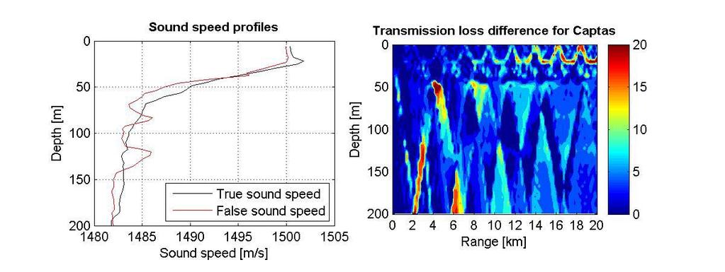
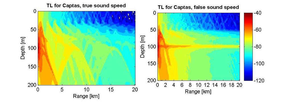
12 10 are used. At 50m and 100m sonar depths, the sonar settings for the CAPTAS variable-depth sonar are used. The one-way transmission loss is modelled, and plotted for two different sound speed profiles. These sound speed profiles are similar in shape and character, but small differences or errors are introduced. The intent is to observe the sensitivity of LYBIN to these changes. One of the sound speed profiles is defined as the true profile, while the other is defined as the false profile (or error-induced profile). The validity of the sound speed profiles is not discussed, just the sensitivity of LYBIN to changes in sound speed. In chapter 4 the sound speed profiles used are presented and discussed. Some of the sound speed profiles are artificial, while others are based on measurements. Figure 3.2 is an example of a figure used in the sensitivity analysis. In the upper left plot, the true and false sound speed profiles are plotted. In this sensitivity analysis we separate between a true sound speed profile, which is the current sound speed profile in the sea, and a false sound speed profile which is different from the current sound speed profile. The two lower plots show the modelled, one-way transmission losses when using the true (left) and false (right) sound speed profiles. The upper right plot is the absolute value of the difference in db of the two sets of modelled transmission losses. Red areas represent areas where the modelled transmission loss is sensitive to the difference in sound speed. The blue areas represent areas where the modelled transmission loss is not sensitive to changes. Figure 3.2: Example of figure used in the sensitivity study.

13 11 4 ENVIRONMENTS Both real and artificial sound speed profiles have been used for this sensitivity analysis. The artificial profiles each reflect nuances of real sound speed profile. The intent is to study errors in each of these nuances by themselves rather than in combination, in order to assess the significance of each type of error. Examples of such nuances are: surface and deep sound channels, and refracting sound speed profiles. All of which are studied in this report. Examples of errors are: depths of sound channels, sound speed gradients of upward or downwards refracting profiles, sound speed minimum in sound channel etc. A selection of these errors is studied. The real sound speed profiles are sets of profiles measured almost simultaneously and in the vicinity of each other. LYBIN should be run with each of the profiles and the results compared in order to find discrepancies and to assess the sensitivity of LYBIN to changes in sound speed. 4.1 Artificial sound speed profiles Three different types of profiles have been constructed. The first is an upward-refracting, constant gradient sound speed profile. The second sound speed profile has a strong surface channel and otherwise an upward-refracting, constant gradient sound speed profile. And the last has a sound channel centred at 100m depth, and a strongly down-refracting upper layer and an upward-refracting lower layer (due to pressure-increase). The types of errors used are as follows: i. Constant shift in the sound speeds vertical gradient, at all depths. ii. Change in minimum sound speed in surface channel. iii. Removal of the deep sound channel (100m depth) Constant gradient Figure 4.1 shows the true and false sound speed profiles using constant gradient. The vertical gradient of the true sound speed profile is 0.015s -1. The false sound speed profile has a vertical gradient of 0.013s -1. This means that the true sound speed profile has a stronger upwardsrefracting effect on the acoustic propagation than the false one.

14 12 Figure 4.1: true and false sound speed profiles using constant gradients Surface channel Two sets of sound speed profiles are presented in this section. The two sets have identical sound speeds below 30m depth, but the surface sound speed and the sound speed gradient within the surface channel varies. In the first example the true surface sound speed is very low, and the false surface sound speed is slightly higher. In this example, the surface sound channel is present both in the true and false sound speed profiles. See Figure 4.2. In the second example the surface sound speed is higher, and the surface sound channel is present in the true sound speed only, not in the false sound speed. See Figure 4.3.

15 13 Figure 4.2: The first set of sound speed profiles with surface channels. Figure 4.3: The second set of sound speed profiles with surface channels.

16 Deep sound channel Figure 4.4shows the true and false sound speed profiles. The true sound speed profile has a significant sound channel centred at 100m depth, while the sound channel is removed in the false sound speed profile. The two sound speed profiles are otherwise identical. It is expected that sources far removed from the sound channel should not be influenced much by the sound channel, but sourced placed within or close to the sound channel will be influenced strongly. Figure 4.4: True and false sound speed profiles with deep sound channel. 4.2 Measured sound speed profiles A single set of measured sound speed profiles are studied. A similar study of a set of sound speed measurements made during the SAT2-tests should be made. Such a study would reveal to what extent spatial or temporal sound speed variation would influence the validity of the acoustic modelling made for the SAT2-tests Poseidon sea trial, September 2005, CTD-line 1 During a sea-trial conducted by the FFI project Poseidon, a series of sound speed profiles were measured along a straight line. Figure 4.5 shows a series of sound speed profiles measured during the trial along a 30km straight line over the course of five hours. The measurements were made at respectively: 02:36, 03:19, 03:57, 04:40, 05:18, 06:08, 06:50 and 07:30 hours. The red sound speed profile was measured at the start of the line. The profiles have all

17 15 the same characteristics; such as a surface channel above a strongly down refracting layer, and finally close to constant sound speed at large depths. In addition some of the profiles have weak deep sound channels at varying depth. Such sound channels are important only if the source or receiver is located within them. Figure 4.5: Measured sound speed profiles along a 30km line. The red sound speed profile was measured at the start of the line. 5 RESULTS In general throughout this chapter, LYBIN has been run with two different sound speed profiles, and the transmission loss results have been compared. The methods of comparison are explained in section 3.1. Generally, we assume that one of the profiles is correct or true, and we seek the error in the transmission loss when using a false sound speed profile. In the case of real measurements, we do not discuss the validity of the sound speed profile, we just define one of the profiles to be true and one to be false. 5.1 Artificial sound speed profiles A few artificial sound speed profiles have been used to illustrate potential errors on a simple level. The sound speed profiles are discussed in section 4.1.

18 Constant gradient Figure 5.1 to Figure 5.3 show the transmission loss and transmission loss difference plots for two LYBIN runs using constant but different sound speed gradients. A hull-mounted sonar at 5m depth is used in the first figure, while a variable-depth sonar at respectively 50m and 100m depth are used in the two subsequent figures. The main discrepancies are along the path of the strongest modes in areas where these modes dominate. Areas where several equally strong modes mix in complex patterns are not sensitive to errors in the sound speed gradient. No discrepancies are seen at short ranges either, since the paths of the propagation modes diverge with increasing range, but are very similar at short ranges regardless of which of the sound speed profiles is used. This is the case for all three source-depths. The long-range discrepancies are largest for deep sources. Figure 5.1: Transmission loss and transmission loss difference plots from LYBIN runs using sound speed profiles with constant but different gradients. Source depth is 5m.

19 17 Figure 5.2: Transmission loss and transmission loss difference plots from LYBIN runs using sound speed profiles with constant but different gradients. Source depth is 50m. Figure 5.3: Transmission loss and transmission loss difference plots from LYBIN runs using sound speed profiles with constant but different gradients. Source depth is 100m.

20 Surface channel Two sets of sound speed profiles are modelled for, presented and discussed. The first set contains a false and a true sound speed profile with different surface sound speeds and gradients but otherwise identical. Both the false and true sound speed profiles have surface channels. In the second example the true sound speed profile has a surface channel, while the false one has too high surface sound speed, and therefore no sound channel. Figure 5.4 and Figure 5.5 show the sound speed profiles, the transmission loss estimate and transmission loss difference for the true and false sound speed in the first example. Since the surface channel is retained, the differences in the transmission loss when using the true and false sound speed profiles are small. This applies both for a deep source (50m) and a shallow source (5m). The exception is that in the deep source case using the true sound speed profile, some rays are caught in the surface layer due to perturbation of ray-paths hitting the surface because of the surface roughness. This does not occur when the surface channel is weakened by the increase of surface sound speed in the false sound speed profile case, causing a discrepancy close to the surface. The effect of ray-angle perturbations in surface reflection is looked into in detail in ref (5). Note that deeper source-depths reduce the discrepancies further, thus deeper sources are less sensitive to changes in surface sound speed. Figure 5.4: Transmission loss and transmission loss difference plots from LYBIN runs using the first set of sound speed profiles with surface channels. Source depth is 5m.

21 19 Figure 5.5: Transmission loss and transmission loss difference plots from LYBIN runs using the first set of sound speed profiles with surface channels. Source depth is 50m. In the second example the surface channel is only present in the true sound speed profile. Figure 5.6 shows that for a shallow source (5m depth), the discrepancy in the transmission loss is significant, especially in the surface layer. When using the true sound speed profile, acoustic energy is caught inside the surface channel and propagates with small propagation loss compared to the bottom-propagating modes escaping the surface channel. The difference in transmission loss in the surface channel therefore increases steadily with range. When using the false sound speed profile, more energy propagates into the depths, resulting in a stronger acoustic field below the sound channel. By using a softer bottom with higher bottom loss, the differences in transmission loss below the surface layer would be less significant since all the modes propagating below the surface channel are bottom interacting. This is due to the high sound speed at the source position. The bottom type used is sand (LYBIN bottom type 2), which has low bottom loss. As expected, Figure 5.7 shows that a deep source is less sensitive to changes in surface sound speed, even if the change in surface sound speed results in the removal of the surface channel.

22 20 Figure 5.6: Transmission loss and transmission loss difference plots from LYBIN runs using the second set of sound speed profiles with surface channels. Source depth is 5m. Figure 5.7: Transmission loss and transmission loss difference plots from LYBIN runs using the second set of sound speed profiles with surface channels. Source depth is 50m.

23 21 All in all, a weakening or strengthening of the surface channel due to changes in the surface temperature, and therefore the surface sound speed, does not influence the predicted transmission loss much. However, if the surface channel vanishes, significant discrepancies are observed if using a hull-mounted sonar, especially in the surface layer. During the SAT2-tests, it is important to measure the surface sound speed continuously when testing the hull-mounted Spherion sonar. However, this is less important when testing the variable-depth CAPTAS sonar, unless the target is at the surface Deep sound channel In this study the true sound speed profile contains a sound channel at 100m depth which is not present in the false sound speed profile. This has little effect on hull-mounted sonars, so the depth-variable sonar, CAPTAS, is modelled for only. Both source depths of 50m and 100m are used. Figure 5.8 shows the transmission loss and transmission loss difference when using the false and true sound speed as shown in the upper right plot. The source is at 50m depth, 50m above the centre axis of the sound channel. For ranges greater than 6km, the difference in transmission loss is mostly insignificant. The exception is due to a change in propagation angle of a bundle of rays leaving the sound channel at approximately 10km range. The change in propagation angle upon leaving the sound channel results in a change in path and therefore a local difference in transmission loss along their path. This is, however not important unless the target happens to be somewhere along the path. This confirms that as long as the source and sonar are placed outside a sound channel, temporal and positional changes in the sound channel do not affect the validity of the transmission loss estimates. This is in accordance with the results in the last section when a surface channel was studied.

24 22 Figure 5.8: Transmission loss and transmission loss difference plots from LYBIN runs using the artificial sound speed profile with a deep sound channel. Source depth is 50m. Figure 5.9 is identical to Figure 5.8, except that the sonar depth is now 100m, at the centre of the sound channel. It is easily seen that the transmission loss patterns as shown in the two lower plots, are widely different in the two cases. When using the true sound speed profile with a sound channel at 100m depth, a large amount of energy is contained within the sound channel. This is obviously not so when using the false sound speed profile. Furthermore, bundles of rays escaping the sound channel have different propagation angles upon leaving the channel when comparing the two modelling results. This results in local differences in transmission loss, but along many ray paths. The sum of all these differences is significant as can be seen in the upper right plot.

25 23 Figure 5.9: Transmission loss and transmission loss difference plots from LYBIN runs using the artificial sound speed profile with a deep sound channel. Source depth is 100m. 5.2 Measured sound speed profiles The sound speed profiles used in this subsection were obtained during a Poseidon sea-trial in September The series of sound speed measurements made is here called CTD-line 1. More information on the sound speed profiles can be found in section We have defined the first sound speed profile along the line as the true sound speed profile, and all the other sound speed profiles have been compared to the first. The resulting plots can be found in appendix A. A few plots are also presented and discussed in this section. Figure 5.10 shows the one-way, modelled transmission loss using the first and second sound speed profile from CTD-line 1. The source is at 50m depth. The two sound speed profiles are very similar in nature; see the upper left plot in the figure. The measurements were made 43 minutes apart. Both have surface channels down to 20m depth, a strong downward refracting profile between 20m and 80m depth and near constant sound speed at greater depths. Consequently the transmission losses are very similar, see the two lower plots in the figure. However, even though the sound speed profiles are similar, there are locally large discrepancies in the results, as seen in the upper right plot. Especially two particular modes of acoustic propagation give rise to discrepancy. The first mode is caught within the surface

26 24 channel. The second is a bottom-reflecting mode. The discrepancies are due to different gradients in the sound speed. Take for instance the bottom-reflecting mode. The true sound speed profile results in a bottom-reflection every 3.5km, while the other sound speed profile results in approximately 4km between each bottom reflection. Since the modes are displaced, large differences in transmission loss appears along both modes, see the upper right plot. The same applies for the mode caught in the surface channel. It is interesting that there is a propagating mode within the surface channel at all, considering that the source is below the surface channel. According to standard ray theory, the source must be placed within a sound channel in order for the sound channel to trap rays. However, LYBIN includes a randomscattering effect at the surface. This effect may perturb the reflection angle of a ray sufficiently to trap it within the surface channel. This effect is discussed in detail in ref (5). Figure 5.10: Transmission loss and transmission loss difference plots from LYBIN runs using the first (true) and second (false) sound speed profile from CTD-line 1 in the Poseidon sea trial. The source is at 50m depth. Figure 5.11 shows the modelled transmission loss along a horizontal line at 50m depth. The upper turning point of the strong bottom interacting mode is at 50m depth. At the turning point rays converge causing a local minimum in transmission loss, and therefore maximum in acoustic energy. Now consider the SAT2 tests, where a single target is used. The resulting measured echo level is then compared to the modelled echo level as based on e g the false

27 25 sound speed profile here. If the target was placed at 50m depth and 14km range, then the error in the modelled one-way transmission loss approaches 20dB. This underlines the importance of: i) Frequent sound speed measurements both at the sonar vessel, between the sonar vessel and target and at the target position. ii) Varying the range between the sonar vessel and the target in order to measure the transmission loss as a function of range. The idea is to confirm whether the target is within a two-ray region, a shadow zone or in the transition zone in between. Figure 5.11: The modelled transmission loss along a horizontal line at 50m depth for both the true and false sound speed profiles. In the second example the source is at 100m depth. The first measured sound speed profile from CTD-line 1 is still used as the true sound speed profile, while the fourth measured sound speed profile is used as the false one. The sound speed profiles are plotted in the upper right plot in Figure The measurements were made 2h and 4 minutes apart. Notice that the false sound speed profile has a sound channel centred at about 100m depth; the source depth. The transmission loss plot to the lower right shows that a large part of the acoustic energy is contained within the sound channel. This as opposed to the true sound speed where there is no

28 sound channel at this depth. The error, as shown in the upper right plot, is great within the sound channel and also along the path of a bottom interacting mode present when using the true sound speed profile, but absent when using the false sound speed profile. 26 Figure 5.12: Transmission loss and transmission loss difference plots from LYBIN runs using the first (true) and fourth (false) sound speed profile from CTD-line 1 in the Poseidon sea trial. The source is at 100m depth. Figure 5.13 shows the modelled transmission loss along a horizontal line at 100m depth. The transmission loss when using the false sound speed profile is slowly varying due to the concentrated acoustic energy within the sound channel. The most important propagation modes in the modelling using the true sound speed profile are bottom-reflecting modes. These modes lose more energy with range due to bottom loss, and they also converge at 100m depth, resulting in local maxima every 7km. The differences in transmission loss are large. Remember also that this is one-way transmission loss, two-way transmission obviously doubles the difference. This shows that sound speed profiles with strong sound channels at the source depth should be handled with care. If long-distance propagation is modelled, then perhaps the sound speed profile should be averaged in order to reduce the effect of temporal or local sound channels.

29 27 Figure 5.13: The modelled transmission loss along a horizontal line at 50m depth for both the true and false sound speed profiles. 6 CONCLUSION The LYBIN estimated transmission loss s sensitivity to changes in sound speed has been studied. Three types of artificial sound speed profiles have been analysed; constant gradient profile, surface channel profile and deep channel profile. In addition a few measured sound speed profiles have been analysed. The intent of the study is to give advice on procedures during the SAT2-tests, in order to avoid problems regarding time- or spatial-varying sound speeds. A potential problem in acoustic modelling is failing to predict the transition zones between two-ray regions and shadow-zones. Two-ray regions are areas where there is a large concentration of rays, while shadow-zones are populated by bottom-reflected rays. One should generally avoid placing the target in such a transition zone. This is also according to the advice given in chapter 3 in ref (4). Obviously, shadow zones should also be avoided.

30 28 Even if the modelled transmission loss states that the target is within an area of stable transmission loss, measures should be taken to confirm this using recorded data. When using a single target of insignificant length, no range-variations are recorded in the echo level (and therefore the transmission loss). If the range is varied, a range variable echo level is recorded, and by assessing the variations in echo level one should be able to determine when the target is within a region of stable transmission loss. According to ref (2), the sonar platform should circle around the stationary target in order to accumulate sufficient statistics on the sonars performance. In most cases, if the target is in the transition zone between a shadow zone and two-ray region, the target should drop in and out of the two-ray region even if the range is held constant. This is due to oceanographic variations. This might enable one to identify whether the target is within the shadow zone, two-ray region or in between. Even so, it is recommended that the sonar platform should follow a straight path while pinging before entering and after leaving the circular path around the stationary target. The measured variations in the measured transmission loss at the target should reveal if the target was within a transition zone during the circular path. If the sonar is placed at a depth susceptible to changes in temperature, either due to changing surface-temperature or currents, then frequent bathy-drops should be made, so as to closely monitor the changes in sound speed at relevant depths. This is especially important when testing the hull-mounted Spherion sonar, though monitoring the surface temperature should be sufficient in that case, since the modelled transmission loss for shallow-depth sonars is not sensitive to changes in deep-water sound speed. The temperature should be monitored from the sonar vessel, at the target position, and if possible at a position between the sonar vessel and the target. If a sound speed measurement reveals the presence of a weak and deep sound channel, one should avoid placing the sonar and target at that depth. Such sound channels are prone to vanish after a time or at a distance. They may be temporal due to deep-water currents or similar. If the sonar is placed in such a sound channel anyways, make sure that frequent bathydrops are made, both from the sonar vessel and at the target position. Such a procedure makes it possible to track the changes in the sound channel. Ref (6) contains a sensitivity analysis of the modelled signal excess varying sound speed profiles as well as wind speed and bottom type. It concludes what depths and ranges the test object should be located to avoid the most sensitive areas.

31 29 APPENDIX A COMPARISON PLOTS, POSEIDON CTD-LINE 1 The following sub-appendices contain comparison plots of the modelled transmission loss using the true and false sound speed profiles obtained from CTD-line 1 in the Poseidon trial, see A.1 Source at 5m depth Transmission loss and transmission loss difference plots from LYBIN runs using the first (true) and N th (false) sound speed profile from CTD-line 1 in the Poseidon sea trial. N runs from two to eight in increasing succession for the seven following figures. The source is at 5m depth.

32 30

33 31

34 32

35 33 A.2 Source at 50m depth Transmission loss and transmission loss difference plots from LYBIN runs using the first (true) and N th (false) sound speed profile from CTD-line 1 in the Poseidon sea trial. N runs from two to eight in increasing succession for the seven following figures. The source is at 50m depth.

36 34

37 35

38 36

39 37 A.3 Source at 100m depth Transmission loss and transmission loss difference plots from LYBIN runs using the first (true) and N th (false) sound speed profile from CTD-line 1 in the Poseidon sea trial. N runs from two to eight in increasing succession for the seven following figures. The source is at 100m depth.

40 38

41 39

42 40

43 41 References (1) Såstad Tale S, Hjelmervik Karl Thomas (2005): LYBIN bottom type analysis, 2005, Restricted (2) Dombestein, Elin M (2004): Summary report of the work done in project 795 New Frigates - work package 1.1 Sonar Performance, 2004/03540, Restricted (3) PPG07 Project 6088 New Frigates (2000): SYSTEM SPESIFICATION FOR THE INTEGRATED WEAPON SYSTEM OF THE NEW FRIGATE (NF), NAVMATCOMNOR, P6088-ABD-SS01202 (4) Knudsen Tor, Dombestein Elin M (2004): SAT 2 test object, required target strengths and source levels, 2004/00250, Restricted (5) Tale S Såstad (2004): The effect of surface roughness in LYBIN simulations, 2004/01269, Restricted (6) Hjelmervik Karl Thomas (2006): SAT2 - LYBINs sensitivity to variations in environmental parameters