How many wheels will it be today?

Transcription

1 How many wheels will it be today? An exploratory research into variables useful for modeling bicycle mode choice with a discrete choice model: master thesis report Jord van der Vliet Supervisors: Prof.dr.ing. Karst Geurs University of Twente Dr. Lissy La Paix Puello University of Twente Ir. Luuk Brederode Goudappel Coffeng

2 Preface This report is the culmination of my education at the University of Twente. It details the activities employed in pursuit of a Master s degree in Civil Engineering and Management, track Traffic and Transport. The research was conducted during an internship at Goudappel Coffeng. First of all, I wish to thank Luuk Brederode for our pleasant cooperation, the very lively and productive discussions, and his many indispensable insights and contributions to this research. Next to him, Dirk Bussche has played a role that is not to be underestimated, from the very first ideas, through respondent recruitment, to the very last bits of data. For this: many thanks. In addition I would like to thank Jantine Boxum for enabling the development and implementation of my survey, and Tjong Cho Wang for quickly fixing problems that showed up at the worst possible time. Karst Geurs deserves my sincere thanks for remaining confident of a positive outcome, despite our troubled cooperation and communication, and for guarding and significantly increasing the scientific value of this research and report. I would also like to thank Lissy La Paix Puello for guarding the technical side of my endeavors. Last, but far from least, I wish to thank the many friends and family that were always willing to listen to my problems and complaints, and to offer advice, during the numerous lows that my graduation process has known. You are the ones that have truly kept me going. 2

3 Abstract To contribute to the modeling of bicycle use in The Netherlands, this research investigates the influences on bicycle mode choice for short-distance commuting. A conceptual model of these influences is defined using available literature. From this, variables are selected for further analysis using a stated preference sample. The sample is collected using a stated choice experiment, in which respondents are asked to choose from presented alternatives in several hypothetical situations. The following variables are included in this research: Attributes Covariates Additional variables Travel time Age Job accessibility Delay Gender Bicycle infrastructure quality Cost Route impression Tabel 0-1: Variables analyzed Income Ethnicity Habit Attitude Workplace policy Workplace facilities The variables are divided into three types: attributes, covariates and additional variables. The attributes are properties of the mode and trip. Covariates are properties of the respondent and his/her workplace. The additional variables are properties of the built environment in the respondent s area of residence. The conclusions drawn from the analysis are: - For bike, the covariates attitude towards cycling, income and especially habit play a very important role in the modeling of bicycle mode choice for short-distance commuting - Travel time is the most important variable for all modes, together with cost for car and public transport - For public transport, in contrast to other modes, job accessibility is important. This reflects the higher service quality of public transport in dense urban areas in The Netherlands - Route-related factors for the bicycle appear to play a very minor role - Delay is of very minor importance for all modes - Age and gender are insignificant - Workplace factors and ethnicity could not be included in the analysis due to sample limitations The weight of these conclusions is significantly limited by the sample size of only 200 respondents. For further research, a larger sample is needed to improve the reliability of the conclusions. In addition, a revealed preference sample will allow calibration of the model used in the analysis, as well as more reliable results. 3

4 Summary In municipal transport planning in The Netherlands, the bicycle has an important place. However, the gravity models currently used to evaluate transport planning measures are not sufficiently capable of modeling bicycle traffic demand. Gravity models cannot include variables such as socio-economic or psychological characteristics, while they are expected to be of influence. The paradigm of discrete choice modeling may provide the necessary capabilities. This leads to the following objective for this research: To contribute to the modeling of bicycle usage in The Netherlands by defining and comparing variables for use in discrete-choice modeling of mode choice concerning short-distance commuting trips. The scope is limited in four ways: - Only mode choice is considered, not route or destination choice, to limit model complexity - Only trips shorter than 15 kilometers are considered, beyond this, cycling is not a reasonable option - Only the trip purpose commuting is considered as this is the primary focus in literature and transport planning - The geographical scope is limited to The Netherlands to provide a reasonably uniform cycling environment To define a theoretical framework, a conceptual model is developed of influences on bicycle use for short-distance commuting. This conceptual model is based on relevant literature and forms the basis of figure 1 (next page). Data for all influences is not readily available, necessitating a data collection method. Two methods are compared: revealed preference and stated preference. Stated preference has the disadvantage that, simply put, people do not behave in the way they say they do. Despite the less reliable representation of average behavior, stated preference is selected as the type of survey to be used. This is because in a stated choice experiment, the researcher controls the variable values in the choice situations, leading to more reliable results for relative parameter importance, which is the information of interest for this research. In addition, stated preference surveys can yield more choice information per respondent. The conceptual model is then used to determine potentially useful variables to include in the data collection. Figure 1 (legend in figure 2) on the next page depicts the conceptual model, with variables selected for analysis highlighted. The variables are divided into three types: attributes, covariates and additional variables. The attributes are properties of the mode and trip. Covariates are properties of the respondent and his/her workplace. The additional variables are properties of the built environment in the respondent s area of residence. 4

5 Natural environment Hilliness Travel time Generalized Cost Monetary cost Built environment Urban form Climate Physical effort Comfort Infrastructure Safety Delay Other modes Travel time Delay Socio-economic factors Age Gender Monetary cost Bicycle use Income Ethnicity Comfort Workplace Company policy Psychological factors Habit Social norms Attitudes Facilities Figure 1: Conceptual model of influences on bicycle use, selected variables highlighted Legend Non-selected variable Selected variable: Attribute Selected variable: Covariate Selected variable: Additional variable Figure 2: Legend to figure 1 Data on attributes and covariates is collected using a stated preference survey, more specifically a stated choice experiment. In such a survey, a respondent is presented with hypothetical situations, and asked to choose from the alternatives listed. Each choice made is known as an observation. Additional questions provide data on the covariates. Respondents to the web-based survey were recruited using company contacts of Goudappel Coffeng, flyering, municipalities in Noord-Brabant and the author s own network. This yielded a sample of 200 responses. 5

6 The sample collected using the survey is then enriched using bicycle network quality data, statistics on urban density and accessibility indicators. This is coupled to the survey data based on the respondent s area of residence. The collected sample is compared to the Dutch working population. This reveals significant problems with regard to size and representativeness: the sample is very small, and has a very different income distribution. This last issue is corrected using weights in the model estimation. Weights alter the importance of observations in a dataset. For example, increasing the importance of observations from respondents with a low income mimics a sample with more low-income respondents. Ethnicity cannot be included as there is no variation in the sample: no persons of non-western origins responded to the survey. Workplace policy and facilities are not included because of irregular early results, which might be due to employees being unaware of policy and facilities available to them. The sample is used to estimate discrete choice models. In a discrete choice model, a decision maker is assumed to choose from a finite number of distinct alternatives. Each alternative has a utility, which is made up of variables, and parameters that describe the importance of the variables. Utility also contains an alternative-specific constant (ASC), this describes the variation in choices that is not described by the variable-parameter pairs. From the utility values of the alternatives, choice probabilities are calculated. The estimated models are corrected for non-representativeness of the sample using weights, and for correlation between multiple observations from one respondent: the survey presents each respondent with nine choices. These nine choices are made by a single person and are therefore not independent. The models used in this research take this into account. The validity of the models is assessed using the value of time they imply for the car and public transport. These values are compared to those obtained in recent research in The Netherlands. The values approach the reference value range closely. The model is therefore considered valid. The results of the estimations are summarized in the figures 3, 4 and 5 (next page). Figure 3 displays the composition of average utility. This is the view an average decision maker has on the different variables analyzed in this research. Figure 4 shows the average choice probabilities for the four modes considered. These are equivalent to the mode shares. Figure 5 compares the influences variables have on the mode share of the bicycle for commuting trips. The values shown are the elasticities of bicycle use for that variable: the percent difference in the bicycle mode share, when that variable is increased by one percent. 6

7 Figure 3: Composition of average utility for the bike, car, public transport and walking. Average choice probabilities Walk; 0,02 Car; 0,17 Bike; 0,64 PT; 0,17 Figure 4: Average choice probabilities (i.e. modal shares) 7

8 Habit ASC Income Attitude Route Delay Travel time Travel time Cost Delay Travel time Cost Delay Job accessibility ASC Travel time ASC 0,60 Variable impact on modal share of bicycle 0,40 0,20 0,00-0,20-0,40 Bike Car PT Walk -0,60-0,80-1,00 Figure 5: Impact of different variables on the mode share of the bicycle for short-distance commuting. The conclusions drawn from this are: - For bike, the covariates attitude towards cycling, income and especially habit play a very important role in the modeling of bicycle mode choice for short-distance commuting - Travel time is the most important variable for all modes, together with cost for car and public transport - For public transport, in contrast to other modes, job accessibility is important. This reflects the higher service quality of public transport in dense urban areas - Route-related factors for the bicycle appear to play a very minor role - Delay is of very minor importance for all modes - Age and gender are insignificant The minor importance of delay may be caused by the way it was incorporated in the survey. Given the mentioned problems with the sample the model is estimated on, the weight of the conclusions is limited. As this research is exploratory in nature, it can still be said that the research goal has been met, but with reservations. The conclusions do reinforce the case for using discrete choice models for modeling short-distance mode choice, as they are capable of including all the variables found to be of influence in this research. In the discussion it is noticed that, while the results mostly agree with earlier Dutch research, they do not agree with foreign research. It becomes clear that the view of cycling and the cycling environment in The Netherlands is very different from that abroad. 8

9 Three recommendations are made: Firstly, a larger and more representative sample will provide a far stronger basis for the conclusions. Secondly, estimating a model on that sample, as well as a revealed preference sample, will yield a calibrated model that can be implemented in transportation modeling, and can be validated. The sample this research is based on was collected using a stated preference method. This is less reliable for average behavior than revealed preference data. Thirdly, the stated choice survey of the type used for this research does not allow the calculation of a value of time for the bicycle or walking, as these costs cannot be directly attributed to a trip. This means that the costs of cycling and walking could not be included in the choice situations of the survey. These values of time are useful in the appraisal of transport-related measures using cost-benefit analysis. Other methods, possibly based on revealed preference data, should be developed as they allow the use of actual costs, including indirect costs. 9

10 Table of contents Preface... 2 Abstract... 3 Summary Introduction Problem description Research objective Theoretical framework Method Method overview Model introduction Data collection method Variable selection Survey design Sample enrichment Sample analysis Model estimation Results Multinomial Logit Mixed logit Model improvements Elasticities Summary of results Conclusions Discussion Weight of conclusions Literature Recommendations Better sample Calibration and validation Cost-benefit analysis Transport planning Bibliography Appendix A: Variables and coding

11 Appendix B: Selected variable histograms Appendix C: Additional model estimation results Appendix D: Priors and levels used for survey optimization Appendix E: Survey

12 1 Introduction An important step in the modeling of transportation is the calculation of the modal split (Ortúzar & Willumsen, 1990). In this step, it is determined what mode of transport a person or group of persons will use to reach their trip s destination. As will be described later in this chapter, the methods currently used in this step are imperfect, when it comes to the inclusion of bicycles. A new method is therefore desired. This research attempts to show what that new method should look like. To do this, a stated preference survey is designed using the state-of-the-art D-efficient design method. The resulting dataset is used to estimate advanced mixed logit models. The resulting parameter values and elasticities give a valuable overview of the impacts of different variables on bicycle use for commuting. The importance of the variables habit and attitude towards cycling found, makes a strong case for the benefits of discrete choice modeling in this context. In this chapter, the problem will firstly be described in some more detail. The second section will introduce the research goal and associated questions. This report will continue with the theoretical framework of influences on bicycle use for commuting in chapter 2. An extensive description of the method employed is given in chapter 3. Chapter 4 presents the results from the model estimations conducted, and chapter 5 contains the conclusions that can be drawn from the model estimations. Chapter 6 discusses the weight that should be attached to these conclusions, and compares them to relevant literature. Finally chapter 7 contains three recommendations for further research and implementation. 1.1 Problem description The first part of the problem description will provide general background information on bicycle usage in the Netherlands. The second part deals with municipal transport planning, the environment in which the model to be estimated in this research is intended to be used. With the background clear, the problems concerning the limitations of currently used models are addressed Bicycle usage in the Netherlands The bicycle has a significant modal share in The Netherlands: 28% of all trips. As bicycles are almost exclusively used for short trips, this constitutes 9% of all kilometers travelled (CBS, 2011). However, short trips are underrepresented in the data, therefore the modal share is probably higher still. The use of electric bicycles, which are used for longer distances, is growing, currently 2 to 4% of commuters use them (Loijen, 2011). Due to the relatively compact nature of Dutch urban areas, the absence of elevation and the high availability of bicycle-specific infrastructure, it can be said that the environment is suitable for cycling (Pucher & Buehler, 2008) Municipal transport planning Dutch municipalities have the obligation to formulate a transport policy, in addition to national and regional plans. Measures for bicycles are explicitly delegated to municipalities by the national government (Ministerie van I&M, 2012). Municipalities are keen to invest in bicycle measures: A main focus for municipalities is achieving a reduction of car use, especially for commuting, to reduce both congestion and pollution. The bicycle is seen as an important and desired alternative (Gemeente Utrecht, 2005; Gemeente Den Haag, 2011; Dienst Infrastructuur Verkeer en Vervoer, 12

13 2012); Municipalities have few funds available, which means that the scale of possible measures is limited. Measures to promote the use of bicycles often sit within this category. Planning for cyclists is therefore an important part of municipal transport planning in The Netherlands. The ex-ante evaluation of bicycle measures is, however, problematic. The municipalities have very little data available on bicycle use; there is a very large uncertainty in the effects of bicycle measures as little research and few ex-post evaluations are carried out; and currently used traffic models cannot cope with bicycles. This means that planning decisions are mostly based on intuition and political sentiment, as well as financial considerations (Keypoint Consultancy, 2012) Model limitations As stated in the previous section, the ex-ante evaluation of bicycle measures is, among other things, hampered by the limitations of traffic models. Currently used models do not explicitly include the bicycle as a mode: they are either unimodal, or include slow traffic as a mode: both walking and cycling combined, as a miscellaneous category. In Dutch urban transportation models, currently used in municipal practice, mode choice and destination choice are usually modeled simultaneously, using a gravity model. The resistances in the skim matrices are calculated in the same way for each mode, and are based on either travel time, trip distance or a combination of both in the form of a generalized cost function. While these attributes are generally sufficient for the modeling of car traffic, they are insufficient for the modeling of slow modes as the bicycle (Krizek, Forsyth, & Baum, 2009): more variables appear to play an important role in the choice to use the bicycle. Inclusion of softer variables as habit and attitudes, or socioeconomic characteristics could improve urban transportation models. Gravity models are not capable of incorporating such variables: each extra variable would double the number of gravity functions needed. A different model type is needed, that can incorporate more and different variables, and that is what this research is to set the first steps towards. Discrete choice models are highly flexible, making them capable of including many different variables such as those mentioned here. Discrete choice models will therefore be the focus of this research. This type of model will be introduced in section

14 1.2 Research objective This section introduces the main objective of the research, with a subsection on limitations to the scope of this research. Additionally, research questions are formulated Main objective The main research objective is defined as follows: To contribute to the modeling of bicycle usage in The Netherlands by defining and comparing variables for use in discrete-choice modeling of mode choice concerning short-distance commuting trips Scope The scope of this research is limited in four ways: Firstly, only mode choice will be considered. Destination choice, mode choice and route choice are linked, and influence one-another (Ortúzar & Willumsen, 1990). However, given practical and temporal constraints, destination and route choice are not included in this research. Secondly, the trip distance considered is limited to 15 kilometers and under. Beyond 15 kilometers, bicycles and walking are no longer relevant alternatives to the car and public transport. Thirdly, only trips conducted with the purpose of commuting will be considered. This is done for two reasons: virtually all literature on bicycle usage is also limited to commuting trips; and for other trip purposes (e.g. recreation), other variables will be relevant in different ways, increasing complexity. Additionally, limiting the research to the trip purpose commuting reduces the heterogeneity of the relevant population, as only the working population is considered. Originally, the geographical scope of this research was limited to the four major cities in The Netherlands: Amsterdam, Rotterdam, The Hague and Utrecht. This was done because of the high similarity in built environment and bicycle use. Due to issues with respondent recruitment, the geographical scope was expanded to include the whole of The Netherlands, to enable the inclusion of all responses in the data sample. This will be described in more detail in subsection Research questions The following questions are formulated to aid meeting the main objective: I. What factors influence bicycle usage for short-distance commuting, according to literature? In the next chapter, a theoretical framework will be built using relevant literature. II. How can data on these influences be collected? For several factors of influence, no data is available. In section 3.3, a method is selected for collection this data. III. What variables should be included in the data collection? The discrete choice model introduced in the previous section allows for the inclusion of many types of variables in many ways. Using the framework of question I, the potentially most useful will be selected in section

15 IV. Is the collected data sample sufficiently reliable for model estimations? A model is only as good as the data it is estimated on. Therefore, the representativeness of the sample must be known and taken into account. V. Which variables are sufficiently relevant for inclusion in a model of bicycle usage for shortdistance commuting trips? For each variable included in a logit model formulation, its relative importance can be calculated. Based on this, variables can be included or rejected. VI. What is the relative importance of these variables for the mode share of the bicycle? By calculating the marginal effects of changes to the variables on the mode share of the bicycle (i.e. elasticities), the importance of the different variables can be compared. 15

16 2 Theoretical framework This chapter introduces the theoretical basis for this research, by building a conceptual model of the factors of influence on bicycle use for short-distance commuting. This conceptual model is compiled and described using relevant literature. It will return in the chapter detailing the method (chapter 3), as a basis for selecting variables for further analysis. The schematic below (figure 6) shows the factors indicated by literature to be of influence on bicycle use, given the trip purpose commuting. The factors are grouped in classes, and the most important interactions are shown. In this section, the factors will be analyzed using the available literature. Natural environment Hilliness Travel time Generalized Cost Monetary cost Built environment Urban form Climate Physical effort Comfort Infrastructure Safety Delay Other modes Travel time Delay Socio-economic factors Age Gender Monetary cost Bicycle use Income Ethnicity Comfort Workplace Company policy Psychological factors Habit Social norms Attitudes Facilities Figure 6: Conceptual model of factors influencing bicycle use for commuting Natural environment The natural environment influences bicycle use in two ways: through the hilliness of the terrain, and the climate (Heinen, van Wee, & Maat, 2010). Both factors do not impact bicycle use directly, but impact the physical effort required for cycling, and the comfort; hence the connection to the generalized cost of cycling. The literature is unanimous on the importance of the hilliness of terrain: the more hilliness, the larger the negative impact on the modal share of the bike (Rietveld & Daniel, 2004; Menghini, Carrasco, Schüssler & Axhausen, 2010; Parkin, Wardman & Page, 2008). The climate affects cycling in different ways, depending on the weather phenomenon considered (Ortúzar, Iacobelli, & Valeze, 2000). Wind increases the required effort, while temperature and precipitation negatively affect comfort. 16

17 Built environment The built environment can be decomposed into two factors: urban form and infrastructure. Two main properties of the urban form are mentioned in literature, and have been used as variables (Rodríguez & Joo, 2004): Urban density (Parkin, Wardman, & Page, 2008) and activity mixture (Pucher & Buehler, 2008). Both properties influence the distance of an average trip, thus the generalized cost of the different modes. As the use of a bicycle is relatively attractive for shorter trips, high urban density and a mix of activities should increase the modal share of bicycles, as they both reduce the average trip length. The infrastructure in an area can significantly impact the modal share of bicycles (Ververs & Ziegelaar, 2006; Pucher & Buehler, 2008). The literature mentions three ways in which the modal share is influenced: its directness, reducing the (relative) distances per trip (Aultman-Hall, Hall, & Baetz, 1997); its quality, increasing both comfort and objective safety (Meng, Taylor, & Holyoak, 2012); and through the number of hindrances and barriers, which increase travel time and decrease comfort (Rietveld & Daniel, 2004). Given the factors mentioned in this paragraph, the built environment is assumed not to influence bicycle use directly, but through the generalized cost of cycling and other modes. This is reflected in figure 6. Generalized cost The generalized cost denotes the perceived cost or discomfort of a trip. The most well-known and omnipresent components are the travel time (including delay) and trip distance (Hunt & Abraham, 2007), and monetary cost. As stated in the subsection on the natural environment, comfort and the physical effort of cycling are relevant factors. In addition, perceived safety is a significant factor (Heinen, van Wee, & Maat, 2010). Perceived safety is here defined as a composite of the objective safety related to accident risk, and more subjective social safety. Both components are considered relevant. Other modes The generalized cost of cycling only really becomes relevant when considered relative to that of competing modes (Rietveld & Daniel, 2004). This means that the components of the generalized cost should also be considered for competing modes, if applicable. In addition, the ownership and/or availability of other modes should be taken into account. Socio-economic factors The socio-economic factors can be broken down to four: age, gender, income and ethnicity (Heinen, van Wee, & Maat, 2010). Age is found to be a significant factor in some studies (Pucher & Buehler, 2008), while others find little or no effect (Wardman, Tight, & Page, 2007). In general, bicycle use can be said to decrease with age, but the relationship is ambiguous (Heinen, van Wee, & Maat, 2010). Gender is less ambiguous: in countries with low levels of bicycle use, men tend to cycle more than women (Rietveld & Daniel, 2004; Rodríguez & Joo, 2004). However, in countries with high rates such as the Netherlands, there is no difference (Pucher & Buehler, 2008). The effect of income is again unclear: as cycling is cheap, one would expect cycling to decrease with income. This does appear to hold for low to middle incomes, but it will rise again with higher incomes. This rise is attributed to a more health-conscious lifestyle. However, not all studies agree on this (Heinen, van Wee, & Maat, 17

18 2010). A factor that does appear to have very clear effects is ethnicity: people of non-western origins tend to cycle much less than other Dutchmen (Rietveld & Daniel, 2004; Harms, 2006). This difference may be explained by a negative attitude towards the bike, hence the link from socio-economic to psychological factors. Psychological factors Three psychological factors are considered relevant: attitudes, social norms (or perceived behavioral control) and habit (Heinen, Maat, & van Wee, 2011). The influence of attitude is relatively straightforward: when a person has a very positive view of the bicycle, that person is more likely to use one. Similarly, when a person s environment views cycling positively, that person is more likely to cycle. This points to the importance of workplace policy, as the workplace is an important environment for an employee, given that this research considers the trip purpose commuting. The inclusion of habit in a mode choice model may also increase its explanatory power (Gardner, 2009). It has to be noted that habit here is not defined as mere frequency, but the degree to which the decision to perform a certain behavior is automatic or thoughtless (Verplanken & Orbell, 2003). Workplace As mentioned in the previous subsection, it makes sense to include factors related to the workplace when considering mode choice for commuting. Two workplace related factors are defined: facilities and policy. Facilities such as covered bike parking spaces, showers and changing rooms can make cycling more attractive, while the availability of car parking space can make the car more attractive (Heinen, Maat, & van Wee, 2013; Hunt & Abraham, 2007). Workplace policy can influence cycling both through the social norms concerning cycling and the (relative) monetary costs (Wardman, Tight, & Page, 2007). 18

19 3 Method The method employed for answering the research questions is detailed in this chapter. As this chapter is large, the first section will give a general overview of the method. In the following sections, the model used (3.2), data collection method (3.3), variable selection (3.4), survey design (3.5), sample enrichment (3.6), sample analysis (3.7) and the model estimation method (3.8) will be described in more detail. 3.1 Method overview In general terms, a discrete choice model will be estimated to obtain parameter estimates. These estimates contain information on the relative importance of variables related to bicycle mode choice. The discrete choice model type will be introduced firstly. Secondly, a data collection method is chosen. The third step is to select variables that merit further investigation. Data on these variables is collected using a survey, and further enriched using other sources. After analysis, the data is the used for model estimations, upon which the conclusions are based. Model introduction In this research, results are obtained using advanced discrete choice modeling. The models and techniques used to improved them need some introducing. The theory, structure, estimation, comparison, assessment and usage will be described. In addition, some improvements to the model are introduced to counter deficiencies in the data sample collected for this research, and weaknesses of basic discrete choice models. The specific procedures used in this research are described in the section on model estimation, section 3.8. Data collection method For many influences on bicycle use, no data is readily available, necessitating the collection of a data sample for this research. Stated preference and revealed preference methods are compared, and stated preference is selected as the type of survey to be developed for this research. Variable selection In chapter 2, the available relevant literature was analyzed for potentially useful variables. These are referenced with the situation in The Netherlands. In addition, the modal alternatives are selected. Survey In the survey, respondents are presented with hypothetical situations, and asked to choose between the presented options. The resulting sample is very useful for estimating discrete choice models (Louvière, Hensher, & Swait, 2000; Ortúzar & Willumsen, 1990). Sample enrichment Data on aggregate variables is more easily and reliably collected from other sources than a survey. The survey sample is enriched using data from CBS statistics, the bicycle network and existing traffic model data. 19

20 Sample analysis As noted in the previous chapter, sample representativeness is important for the model s reliability, and therefore the weight of the conclusions of this research. The sample is analyzed and compared to a reference population. Model estimation The sample data is used to estimate parameter values, that denote the relative importance of the associated variables. Upon this information, the conclusions are based. 20

21 3.2 Model introduction The model type that will be used in this research is the highly flexible discrete choice model. In this section, this type of model will be introduced and analyzed, based on the books Modelling Transport (Ortúzar & Willumsen, 1990) and Discrete choice models with simulation (Train, 2003). Firstly, the theory of utility maximization, on which discrete choice modeling is based, will be introduced. The structure of the multinomial logit (MNL) model is then described. The subsequent subsections detail the estimation, comparison and assessment of logit models. The applications and weaknesses are also discussed. To resolve the weaknesses of the MNL model, mixed logit and two model improvements are introduced Utility maximization Discrete choice models aim to describe the choice process of a decision maker. This decision maker is assumed to choose from a finite choice set of discrete and mutually exclusive alternatives. This means that all alternatives are defined, and that the decision maker may only choose one of them. The theory of utility maximization states that a decision maker will consider the relative benefit of each alternative. This is defined as utility. Note that this utility can also be negative. In fact, it has no scale or relevance on its own, only when compared to the utility of other alternatives. The decision maker will then choose the alternative with the highest utility. In reality, people do not behave completely rationally, requiring a probabilistic instead of a deterministic approach MNL structure The most basic and widely used discrete choice model is the multinomial logit (MNL). Its structure consists of two types of functions: the utility function and the logit function. The utility function again consists of two parts: the observed part, and the random part. The observed part of utility for decision maker n and alternative i is represented by a linear combination of variables as defined by the researcher: Where vector x denotes the variables, and the vector consists of estimated parameters that determine the relative importance of the variables for alternative i. The function also includes a term that captures the rest of the of the observed utility. This term is known as the alternative-specific constant (ASC). As the overall scale of utility is irrelevant, the ASC of one alternative is normalized to zero. To include the mentioned probabilistic approach, a random component function: is added to the utility This error term captures the unobserved parts of utility. In the case of and MNL it is assumed to be independently, identically distributed extreme value. The choice probabilities are derived from the utility values using a logit function. The probability for decision maker n to select alternative is defined as: 21

22 This leads to the relationship between choice probability and utility value as depicted in the following graph: Figure 7: Logit function (Train, 2003, p. 38) Maximum likelihood estimation Logit model parameters are estimated using maximum likelihood estimation. This revolves around a measure of fit to the dataset used for estimation: the likelihood that this particular dataset emerges given a specific set of parameters (i.e. model estimate). A log-likelihood function is defined as the natural logarithm of that likelihood, as a function of a vector β t containing the parameter estimates, as depicted in figure 6. A model fit is considered optimal ( ) when the log-likelihood is at a global maximum. Therefore, estimating a model is equivalent to optimizing the log-likelihood function. The log-likelihood function takes the availability of an alternative to a respondent into account. Figure 8: Maximum likelihood estimate (Train, 2003, p. 186) 1 1 This graph shows a hypothetical log-likelihood function for a single element vector β (corresponding to a model with one parameter) 22

23 3.2.4 Model comparison and assessment Logit models are developed iteratively: one starts with a basic model that only includes alternative specific constants, and then adds variables (and their parameters) one by one. It has to be noted that the addition of more variables does not necessarily make a model better. A goodness-of-fit statistic is therefore needed to compare consecutive model estimations. The most often used statistic is the likelihood ratio index ρ 2 (Train, 2003): Where is the value of the log-likelihood function at the estimated parameters and is its value when all parameters are set equal to zero. When comparing models one must adjust for the difference in number of variables between them (Bliemer, 2013). This adjusted likelihood ratio index is used in this research to compare model estimations. The use of the likelihood ratio index has the limitation that models must be estimated on the same dataset. The use of weights to correct a dataset, as will be done in this research, will yield a different dataset. Models estimated on weighted and unweighted datasets can therefore not be compared on the basis of a likelihood ratio index. On a parameter level, a t-test is used to determine whether that parameter makes a significant contribution to the fit of the model. A parameter that is significant, shows that the associated variable has explanatory value given the model form used. That variable-parameter combination is then used in subsequent model estimations, while non-significant parameters and associated variables are removed from the model. A reverse-order estimation procedure is also employed: one estimates a model that includes all variables, and then removes the insignificant variables one by one. Ratios between parameters that have a meaning by themselves can be used to give an indication of the model s validity. The value of time is most often used. This is the ratio between the parameter for cost and that for time, adjusted to cost per hour. This value is interpreted as the willingness to pay for travel time reduction. The validity is assessed by comparing the value to that in relevant literature Application As shown in subsection 3.2.2, the structure of the utility function in a discrete choice model is highly flexible, allowing inclusion of many different variables. Discrete choice models are often used for the modeling of mode choice, as this choice involves many variables. It is suggested as a potentially superior method for modeling bicycle and pedestrian travel (Porter, Suhrbier, & Schwartz, 1999). In this research, discrete choice modeling is applied to derive the relative importance of variables from estimated parameters. 23

24 3.2.6 Weaknesses Assuming that the error terms are independently, identically distributed (IID) creates a potential weakness. The assumption implies that all observations are independent from one-another. When using survey data, where respondents often each supply multiple observations, this does not hold. The next subsection explains how this can be dealt with. The MNL has another weakness, which occurs when alternatives are correlated. It has a property known as independence of irrelevant alternatives (IIA): when an alternative is added, the relative probabilities for the existing alternatives do not change. This means that the probabilities for correlated alternatives are overestimated. A solution to this, is to nest correlated alternatives, and use a compound utility in the higher level. This method is known as nested logit. The alternatives (modes) used in this research (see subsection 3.4.3) are not expected to be correlated, as they constitute clearly separate modes of transport. There is therefore no reason to expect the independence of irrelevant alternatives property to be an issue Mixed logit In a multinomial logit model, the random component of utility is represented by an error term that is independently and identically distributed (IID) extreme value across observations. However, the assumption of independence does not hold in the case of panel data: each respondent makes a choice in multiple scenarios, and therefore yields multiple observations, instead of just one. Those observations are not independent: they were made by the same individual. The mixed logit model offers a way of correcting for this. The mixed logit model was originally developed to account for random taste variations between respondents, using random parameters. However, these random parameters are formally equivalent to error components, which can be used to account for the correlations between observations from the same respondent. Structure The general functional form of the mixed logit model is the same as that of the MNL, as depicted in subsection The parameters β, however, are not fixed, but drawn from a distribution defined by the researcher. The random parameters β themselves are no longer estimated, rather the parameters of their distribution θ are. The probability is given by the logit probability, integrated over the possible values of β, as defined by the estimate of θ (i.e. the mixing distribution, hence the name mixed logit). This yields the following structure: For this research, the interest is in error components. These are obtained by detaching the distribution θ from the parameters β, and instead applying it to the error components. These error components are distributed normally across respondents, with zero mean and have an estimated standard deviation θ. The structure is now as follows: 24

25 The error components account for the correlation between the observations of a single respondent, as they vary over respondents, and not over observations for any single respondent. Simulation As the probability is now dependent on a distribution, it cannot be calculated directly, which was the case with the MNL model. Instead, simulation is used in forecasting and estimation: values are drawn from a specified distribution (in the case of panel error components: the normal distribution), and the logit probability is calculated using those values. The average is then the simulated probability : Where denotes the draw from the distribution, and is the total number of draws Model improvements In addition to the error components of mixed logit, two techniques will be employed to further improve the model estimated in this research. This subsection will introduce effects coding and weights. Effects coding In a utility function, each variable is preceded by a single estimated parameter that describes its importance within the model. A single parameter can only describe a linear relationship between a variable and its effect on utility. However, for some variables it may better not to assume that relationship to be linear. Non-linear effects can be captured using effects coding (Bliemer, 2013). This is done by dividing the value range of a variable into N classes, and then use N-1 parameters to describe the effects on utility per class. This is illustrated with an example 2 : Considering the choice of airline flights, one looks at the effect of departure time on utility. By estimating a single parameter, one assumes that the relationship between departure time and utility is linear. The parameter value resulting from estimation will describe a relationship as depicted below: Figure 9: Relationship between utility and departure time for airline flights (Bliemer, 2013, p. 112) 2 Based on: Executive course: Discrete Choice analysis & Stated Choice Experimental Design (Bliemer, 2013, pp ) 25

26 In effect, one is assuming that later flights are preferred over earlier flights. A non-linear relationship is captured by defining not one normal variable, but four dummy variables: one per class, that is one when the normal variable has the value of that class, and is zero otherwise. For each dummy variable, a parameter (A-D) is estimated: Departure time 6am 10am 2pm 6pm A B C D Table 3-1: Dummy coding scheme Effects coding is a more efficient way of doing the same thing. As the absolute scale of utility is irrelevant (only differences matter), one should remove one dummy parameter. In dummy coding, this would mean losing information on one of the variable classes. Effects coding prevents this by using the following coding scheme: Departure time 6am 10am 2pm 6pm A B C Table 3-2: Effects coding scheme Figure 10: Relationship between departure time and utility when using effects coding (Bliemer, 2013, p. 115) It is clear that the relationship between departure time and utility is not in fact linear. Note that this model was estimated on the same data. Weights A logit model is estimated on a data sample, from a target population. It is not uncommon in practice that a sample is an imperfect representation of that target population. This research is no exception. As a model estimation is no better than the data it is estimated on, this non-representativeness must be addressed. To correct for this, weights can be added to the dataset for each respondent, which alter the importance of relevant observations in the likelihood function described in subsection For example: a respondent with a low income is designated a weight greater than one, making the observations from that respondent more important, mimicking a dataset with more low-income respondents. 26

27 3.3 Data collection method For several factors mentioned in the conceptual model, most notably psychological factors and workplace factors, no data is available to estimate models on. This data must therefore be collected for this research. There are two methods by which this can be done: revealed preference (RP), and stated preference (SP). This section compares the two, and selects the one most suited to this research Revealed preference In a revealed preference survey, respondents are asked to report the choices they have made. A respondent, for instance, reports having used the bike to go work that day. This trip was 5 kilometers, and took him/her 20 minutes. This type of survey accurately captures the actual behavior of respondents, which in modeling terms translates into accurate values for the alternative-specific constants (ASCs) in a utility function (Train, 2003). However, RP has three drawbacks: Firstly, the data sample can only describe current behavior, as respondents report their actual behavior. Data can therefore not be gathered on alternatives or situations that do not (normally) exist. In this research, only current and normal alternatives and situations will be considered, this drawback is therefore not an issue. A second drawback is an issue: the variation in the variables is not controlled for, which means that some key variables may not exhibit sufficient variation for modeling. In general terms, RP data describes average choices well, but the relative importance of variables less so (Train, 2003). Thirdly, data form an RP survey gives information on the choices that respondents made, but no information on the alternatives they did not choose. This information is required for the estimation of discrete choice models, as choice probabilities are computed using data on all alternatives (see subsection 3.2.3) Stated preference A stated preference survey, more specifically a stated choice experiment, presents respondents with one or more hypothetical situations. In these choice situations, alternatives are described, and the respondent is asked to state which of the alternatives he or she would choose in reality. Figure 13 in subsection contains an example of a choice situation from the stated choice experiment developed for this research. The large drawback SP data has, is that respondents make hypothetical choices from hypothetical alternatives. This makes the data less realistic than RP data, especially in terms of average behavior, reflected in the alternative-specific constants (Train, 2003). In contrast, the researcher controls the variable variance, as the variable values (in this context called levels) are part of the choice situation design. The relative importance of variables is therefore better derived from SP data, which is precisely the goal of this research. In addition, it is standard practice to include multiple choice situations in a survey (Louvière, Hensher, & Swait, 2000), and thereby gaining more observations per respondent. Given the advantages an SP survey has over RP in the case of this research, this is the data collection method chosen. The SP survey design is described in section

28 3.4 Variable selection Before a survey and further data collection can be designed, the data required from it must be determined. In this section, the conceptual model of influences on bicycle use is analyzed and used to determine the variables of interest. These variables are then summarized in an overview. Additionally, the modal alternatives to be considered are determined Selected variables Natural environment The climate in The Netherlands is temperate and fairly uniform across the small country (KNMI, 2011). Assuming climate influences the propensity to cycle, this is highly unlikely to be reflected in the data collected for this research, and therefore is not a useful variable: the variability in climate in The Netherlands is so small that a very large number of respondents from across the country would be needed to discern significant influences. Nor would the resulting data be useful in traffic modeling within The Netherlands: as the climate between areas is the same, it cannot account for any differences in bicycle use. A similar argument applies to the hilliness of the country: apart from an area in the south, there is virtually no hilliness in the country, especially not in the four major cities, which were the original focus of this research. Built environment The car infrastructure in The Netherlands is subject to relatively strict guidelines, and therefore does not show much variation. This is not so much the case for bicycles, that infrastructure shows more variation, making this a potentially useful variable. The public transport network also shows variation: in dense urban areas, the service quality is better, as there is more ridership there. Urban density may therefore be a useful variable. A variable that can capture both the directness and quality of service of the infrastructure and the destination density is accessibility. This may in part explain modal choice, making it a potentially useful variable. Generalized cost Given the assumption of invariance for the natural environment made earlier, the physical effort of cycling will be directly correlated with the travel time. It is therefore not useful to include both variables. As travel time is the more objectively measurable of the two, this variable will be used. Safety is only in part objective, which makes it more useful to consider the attitude towards the safety of cycling than to look at objective components of safety, such as accident risk. The same argument applies to comfort, as this is also highly subjective. The monetary cost of cycling is small. As the only real costs are the purchase and maintenance of a bike, a trip does not cost anything in itself (the out-of-pocket cost). Cycling is effectively perceived to be free. The costs for cycling will therefore be ignored in this research. Other modes In contrast to cycling, out-of-pocket costs do apply to the car and public transport. These will be included in the data collection. The arguments employed with respect to comfort and safety apply not only to cycling, but also to other modes. 28

29 Socio-economic factors Of the four socio-economic factors mentioned, the influence of age and income is uncertain. It will therefore be especially useful to include these variables. Gender is probably not useful, but it is very easily included. Ethnicity is an important variable, but data collection will be an issue as relatively few people of non-western origins will complete a survey. Psychological factors Even though psychological factors do not lend themselves for aggregation, and data on them does not exist, including them may yield useful insights. It is attainable to include both habit and attitude towards cycling in a survey. Workplace Workplace factors are again difficult to aggregate, unless they are the result of higher level planning. But including both facilities and policy may yield useful insights for mobility planning. 29

30 3.4.2 Overview The figure below is the conceptual model introduced earlier, with the selected variables highlighted. A legend is provided in figure 11. The variables are divided into three types: attributes, covariates and additional variables. The attributes are properties of the mode and trip. These will be included in the choice situations in the survey. Covariates are properties of the respondent and his/her workplace. The information on these will be collected using extra questions in the survey. The design of the survey is the subject of the next section (3.5). The additional variables are properties of the built environment. The data on these variables is gathered from other sources and is matched to the respondent s area of residence. The method, with which this is done, is described in section 3.6. Natural environment Hilliness Travel time Generalized Cost Monetary cost Built environment Urban form Climate Physical effort Comfort Infrastructure Safety Delay Other modes Travel time Delay Socio-economic factors Age Gender Monetary cost Bicycle use Income Ethnicity Comfort Workplace Company policy Psycholigical factors Habit Social norms Attitudes Facilities Figure 11: Conceptual model of factors influencing bicycle use for commuting, with selected variables highlighted Legend Non-selected variable Attribute Covariate Additional variable Figure 12: Legend to figure 11 30

31 3.4.3 Modal alternatives Even though there is no theoretical limitation to the number of alternatives in a discrete choice model, there are practical restrictions in terms of survey length and complexity. Of these restrictions, survey complexity is the limiting factor. The more alternatives in a choice scenario, the harder it is for a respondent to make a choice. Complexity is therefore roughly inversely proportional to reliability. In addition, more alternatives leads to more parameters to be estimated in modeling, while the amount of choice data does not increase given the same number of respondents. More alternatives therefore means more respondents are required (Bliemer, 2013). For these reasons, and responses to the pilot survey (see subsection 3.5.5), the number of alternatives is limited to four. In addition to the bicycle, the alternatives will be car, public transport and walking. Again for simplicity, public transport is defined as bus, tram and metro, not including train. A train trip is often longer than 15 kilometers, the limit of the scope of this research. Additionally, a train trip usually includes access and egress legs, which would introduce too much complexity. The train is therefore not considered as an alternative. 31

32 3.5 Survey design The data gathering method for the attributes and covariates used in this research is the statedpreference survey, as determined in section 3.3. This section details the design of that survey, starting with the design considerations. The survey components that deal with a recent reference trip, the stated choice experiment, and the covariates are then discussed. In addition, the pilot survey and the respondent recruitment are described. The resulting survey can be found in appendix E, the definitions and coding of all variables in appendix A Design considerations Before designing the survey, two aspects were considered: error sources and the targeted respondents. This section will describe how targeting and error sources, if applicable, will be taken into account. Error sources An important factor to take into account during survey design, is a selection of error types in surveys: respondent fatigue, policy response bias and self-selectivity bias 3 (Bates, 1988). To prevent fatigue issues, the maximum survey length is set at ten minutes, based on the experience of experts at Goudappel. Policy response bias refers to the possibility that respondents alter their responses in such a way as to actively influence the outcome of the analysis. This is not expected to be an issue in this survey, as respondents have no stake in the outcome of this research. What may be an issue, is that cycling is socially and individually preferable over motorized transport. This will at times result in respondents choosing the bicycle, while in reality, given the same situation, another mode would have been selected. Targeted respondents Given that the scope of this research is limited to the trip purpose commuting, the survey will be aimed at employees. Pre-selection questions are therefore included in the survey, to insure that only respondents that are employed and do not work from home can fill out the survey. As there is no budget available for an incentive or a panel, the survey should be as little a burden as possible. For this reason, the survey is anonymous and relatively short Recent trip The actual survey starts with a series of questions about the last commute trip the respondent made. This is important for the framing of the choice scenarios: the goal is to make them as realistic as possible (Bliemer & Rose, 2005). Reminding a respondent of a recent trip will help that respondent to relate the scenarios to his/her own situation. The questions also serve a further purpose: respondents are asked for their residential location, which will be used for the addition of extra variables from other data sources (see section 3.6). In addition, the estimated trip distance will be used to assign a respondent to one of three distance bins (see next subsection). 3 Also commonly known as justification bias 32

33 Should the respondent fill in a trip length that is longer than the limit defined in the scope of this research (15 km.), he/she is then asked to bring another trip (with another purpose if need be) to mind that is shorter. It would be preferable to remove such respondents from the sample, as the choice scenarios do not relate to their reality. This was, however, not an option due to the low total number of respondents in the final sample (see section 3.7). Lastly, respondents will be asked whether they have a car available for commuting, so that the car alternative can be removed from the scenarios for those to whom it is not available in reality. This is again done to increase realism Stated choice experiment The stated choice experiment is the core of the survey. Respondents are presented with hypothetical scenarios, and are asked to choose from the available alternatives based on the mentioned properties (attributes). The goal is to provide the choice data for the attributes as described in section 3.4. The first step in the design of the scenarios is the selection of priors and levels. The values of the attributes in the scenarios that respondents can use to base their choices on, are called levels. For optimization, it is needed to guess the relative importance of the attributes. This will allow the optimization algorithm to estimate the information value of a choice set. These guesses are called priors. The levels are arranged into choice sets, and optimized for the maximum amount of information per choice per respondent using the priors. Lastly, the optimized choice sets are visualized for inclusion in the survey. Priors and levels The levels must be selected carefully (Bliemer, 2013), as they both determine the realism and the information richness of the scenarios. For maximum information richness, the levels for any attribute should be as widely spaced as possible, but this may lead to unrealistic scenarios. Therefore, a tradeoff must be made by the designer. Another requirement for realism, is that the scenarios are close to the reference of the respondent, as the goal is to get the respondent to make the same choice as he/she would have made in reality. For this reason, not one, but three sets of nine scenarios each are designed. A short set (1-3 km.), a medium set (4-7 km.) and a longer set (8-12 km.). The priors used in this design were educated guesses, based on: earlier experiences with discrete choice modeling at Goudappel (Brederode, 2010); values of time from recent research in The Netherlands (Rijkswaterstaat, 2011); and the results of the pilot survey (see subsection 3.5.5). The actual priors and levels used can be found in appendix D. Optimization of choice sets The levels are arranged into choice sets, and optimized using the priors following the D-efficient design method. This method has been shown to be superior to the direct alternatives such as an orthogonal survey design (Rose, Bliemer, Hensher, & Collins, 2008). The method revolves around the minimization of the D-error. This D-error is the determinant of the asymptotic variance-covariance matrix of parameter estimates (priors) (Bliemer & Rose, 2005). The lower this D-error, the more 33

34 efficient the design. The asymptotic variance-covariance matrix is computed as the second derivative of the log-likelihood function as described in subsection 3.2.3, using the priors and levels. The optimization was done within the ngene software package (Choice Metrics, 2011). Two constraints were added to retain realism and variety: the car travel time in any scenario has to be shorter than that for bike, not including delay; and each attribute level can only be used 2 to 4 times. This last constraint was needed because the algorithm has a tendency to use only the most extreme levels. A restriction of the method is that the number of scenarios per set must be a multiple of the number of levels per attribute. As the number of levels is determined at 3, each set is made up of 9 scenarios, as 12 scenarios would have resulted in too long a survey. Presentation in survey The following figure shows an example scenario from the final survey, with English annotations. This scenario is also used as an example in the actual survey for the medium distance bin, with annotations in Dutch. Each distance bin has its own example, and the car alternative is removed if not available to the respondent, just as in the actual scenarios. Figure 13: Example choice scenario, in the original Dutch with English annotations Each scenario is followed by the question which mode the respondent would choose to travel to work. After selection, the respondent can tick the box I would not travel given these alternatives. This would be an indication that the scenario is unrealistic 4. 4 This option was not used by any respondent. 34

35 The alternatives and their attributes are presented in a table, as a more graphic representation would be too cluttered and confusing. Icons are used to further clarify the alternatives. The levels of the bike route impression are represented in picture form, with pictures denoting a bike path (good, pictured in example), a busy street with bike lanes (mediocre) and a very busy street without any facilities (poor). Figure 15: Mediocre route impression Figure 14: Poor route impression Further survey questions Data on socio-economic and psychological variables (covariates) is gathered in that latter part of the survey. These questions deal with: habit, attitude, workplace and personal information. Information on the coding used for these variables is included in appendix A. The survey questions themselves can be found in the survey in appendix E. Habit For the inclusion of cycling habit, the self-reporting habit index (SRHI) as introduced by Verplanken and Orbell (2003) is used. This scale has been used for studying habit in physical exercise (Verplanken & Melkevik, 2008) and in mode choice modeling (Gardner, 2009). It conforms to the concept of habit as it is used in this research: not just the frequency, but the degree of automatism of the behavior. The question consists of 10 statements, for which respondents can state the degree of applicability using a five-option Likert scale. Attitude The attitude towards cycling is captured analogous to recent research conducted by Heinen, Maat and van Wee (2011). The question has however been reduced in size and simplified because of survey length concerns. The question consists of 14 statements, similar to the SRHI, again with a fiveoption Likert scale. Workplace Respondents are asked whether certain facilities are available to them at their workplace, and whether certain policies are applicable. The facilities considered are: parking facilities for bike, moped and car; showers; and changing room. The policies are: positive financial stimulation (purchase subsidies, or travel cost reimbursement); negative financial stimulation (paid parking); and the provision of a company car or a free public transport pass. 35

36 Respondent information Lastly, respondents are asked to fill in personal information: their age, gender, ethnic origin and income Pilot survey A pilot survey was executed to test the formulation of the questions, a preliminary design for the scenarios and to provide better guesses for the priors. This subsection discusses the pilot survey design, its execution and the adjustments made based on the pilot survey results. Design The pilot survey is based on a simplified preliminary design for the final survey. This was done to enable execution of the pilot survey earlier in the design process. Only a single distance bin was used, and the example, pre-selection questions and the route impression were omitted, as they had not yet been developed. Execution The pilot survey was implemented as a web survey, using the Snap software (Snap Surveys, 2009). An invite was sent to two departments within Goudappel: Research & Development and Supporting staff, in total roughly 40 persons. This was done to have both critics and outsiders look at the pilot. Of those invited, 15 responded (excluding tests). With this small sample, a basic model was estimated, using the method described in sections 3.2 and 3.8. Results and adjustments It quickly became apparent that the survey software would only send results after a respondent fully completed the survey, and that it is impossible to determine where a respondent stopped when he/she did not fully complete the survey. This information would have helped identify questions that respondents dislike. Due to limitations in the Snap software, and no access to server log files, this issue could not be fixed. The resulting parameter estimates from the basic model were used to update the priors for the optimization of the final survey: walking was made more attractive; the ASC prior for bike was made positive (from zero) and the ASC for public transport was made zero (from negative). These adjustments greatly improved the generated choice scenarios. The basic model also indicated that the delay was indistinguishable from travel time. Apparently, respondents would simply add the two numbers, or ignore the delay. To deal with this, the instructions were clarified, and a + sign was used to indicate that the delay is not part of the travel time. It was considered to show the delay level in red, but this would probably cause respondents to focus primarily on that attribute in the choice process, inducing lexicographic behavior (Train, 2003). The most common comment on the pilot survey was that the choices were difficult, because the scenarios were not representative of the respondent s own situation. This affirmed the need for three different distance bins. 36

37 3.5.6 Respondent recruitment The final survey was, just as the pilot, implemented in the form of a web survey using Snap software. This subsection describes the way respondents were recruited for this research, and the changes made to the geographical scope. Initially, the geographical scope of this research was defined as the four major cities in The Netherlands: Amsterdam, Rotterdam, The Hague and Utrecht. Together with their satellite towns, these cities form the urban agglomeration known as the Randstad. This scope was chosen as these cities have a comparable built environment in terms of density, infrastructure and activity mixture. Additionally, the cities have high rates of bicycle usage, and their local governments are interested in evaluating bicycle-related transport measures. Invites for participation were firstly sent to employees of Goudappel Coffeng (offices in The Hague and Amsterdam), and to contacts from Goudappel at Rijkswaterstaat (Utrecht office) and at U15 (Utrecht). From Goudappel, 8 employees from the Amsterdam office responded, and 10 from The Hague. The contacts at Rijkswaterstaat and U15 did not properly forward the invitation, this yielded only 5 respondents. As this sample size of 23 is far too small, flyering was attempted at the bus stop Rijnsweerd Noord in Utrecht. This bus stop is located in a commercial area, where many employees alight during the morning peak. The flyering was abandoned after one day, due to a response rate of less than 3%: only 7 respondents were recruited, while 250 flyers were handed out. A response rate of 10-20% was expected. This failure is probably due to the fact that no incentive was offered, and that respondents had no connection with, or stake in, the outcomes of the survey. At this point, the decision was made to widen the geographical scope of the research. The reference population is larger and more diverse (as well as the built environment), requiring a larger sample. However, the widened scope provided the opportunity to recruit respondents from more sources: Responses from the Goudappel Deventer head office could now be used (51), and via contacts at Goudappel, the NHTV Breda offered the use of its panel in Noord-Brabant. Unfortunately, the panel could not be used: it is owned by the province of Noord-Brabant, but is managed by a private company. This private company required the use of its own survey systems, which in turn required a redesign of the survey. The survey is large, and uses several dynamic elements. There were no funds or time available to allow the company to make the conversion. Online panels such as Survey Monkey and Thesis Tools were also rejected, as they too required a survey redesign for their own systems. Source Respondents Goudappel 69 Company contacts 5 Flyering 7 Municipalities 52 Other 67 Total 200 Table 3-3:Respondent sources After the use of these panels fell through, the NHTV Breda contacted the municipalities of Den Bosch, Eindhoven and Breda. This yielded 52 respondents (29; 9; and 14). Lastly, the author used his own network, yielding a further 67 respondents, for a total of 200. The respondent sources are summarized in table

38 It has to be noted that the survey is anonymous: respondent numbers from the different sources are inferred based on the time of response and origin and destination postal codes. This means that the numbers in table 3-3 may not all be correct. 3.6 Sample enrichment The survey alone does not provide all the data wanted for this research: respondents were not asked for information on the built environment, as this is more reliably collected using available data. This section deals with the enrichment of the survey sample with data based on the respondents residential location. Three types of variables are added: urban density, accessibility indicators and bicycle network quality indicators. A description of variable coding is included in appendix A Urban density Urban density is derived from CBS neighborhood statistics (CBS, 2012), where it is defined as the number of addresses per square kilometer. The data is aggregated to postcode-4 level, and assigned to respondents based on the postcode-4 of their residential location, as entered in the survey. The CBS data used does not contain the actual address density, but divides it into five classes. Those same classes are used in this research Accessibility The accessibility indicators are derived from the database behind the Goudappel Coffeng Bereikbaarheidskaart (Goudappel Coffeng, 2011a), which is in turn based on travel times from the National Transport Model (NVM; van der Griendt & Palm, 2011). For bike, travel times were obtained from the Twente Mobiel bike route planner (Goudappel Coffeng, 2011b). To obtain an accessibility indicator, a contour of 30 minutes travel time is used (45 minutes for bike), which is the longest trip length that features in the choice scenarios in the survey. The travel times for car and PT were generated for the 2008 base year, during the morning rush, including congestion. The indicator itself is the number of jobs within the contour. These numbers are, however, too large to be used in modelling directly: As shown in subsection 3.2.2, the effect of a variable on the utility of a mode (and thereby probability) is determined by a parameter. If the values of a variable are very large (in this case: tens of thousands), the parameters will be estimated to be very small indeed 5. A test of parameter significance, as mentioned in subsection 3.2.4, revolves around a t-test that gives the probability that the parameter is zero. When that parameter is very small, it will more likely be insignificantly different from zero. Therefore, instead of using the actual number of jobs, the natural logarithm is used Bicycle network quality The Dutch Cyclists Union maintains a bike route planner, that allows members to add information concerning network quality to the links in its network (Fietsersbond, 2013). This link-level data was aggregated to postcode-4 level by assigning each link to a postcode-4 zone, and summarizing the length of all links that conform to each level of all variables per postcode-4 zone. From this data four indicators are developed: infrastructure quality, hindrance, lighting and surroundings. 5 Assuming that the influence of the variable on utility is of reasonable proportions. 38

39 The infrastructure quality is composed of a score for the type of road surface, and its state of maintenance. Hindrance is defined as (a score for) the amount of traffic on a link that interferes with cyclists on that link. Lighting is the degree to which the link is lit by street lighting, and the surroundings indicator is a score for the beauty of the link s surroundings. It has to be noted that the data was collected by volunteers from the Dutch Cyclists Union. Much of the data is subjective, and there is a significant amount of missing values (roughly 12% for most variables). The missing values were dealt with by making the lengths of relevant links, per variable level, per postcode-4 zone, relative to the total zone network length, minus the length of links with missing values. This effectively removes the links with missing values from the dataset. 39

40 3.7 Sample analysis In this section, the sample collected using the survey will be described. Secondly, the sample is compared to a reference population, to determine the representativeness of the sample. In addition, the usability of data on workplace facilities and policy is discussed. Variable definitions and coding can be found in appendix A Sample statistics The sample consists of 216 responses, of which 200 are useful (yielding 1800 observations). The geographical spread of the respondents is shown in table 3-5. It is far from uniform: Overijssel and Noord-Brabant together make up close to 50% of respondents. This is a cause for concern considering sample representativeness, which will be addressed in the next subsection. The distribution across distance classes in the survey, based on respondent s reference trips, is fairly uniform. It is shown in table 3-4. Province N % Overijssel 44 22% Gelderland 37 19% Zeeland 23 12% Noord-Brabant 49 25% Utrecht 13 7% Zuid-Holland 18 9% Noord-Holland 8 4% Flevoland 5 3% Drenthe 0 0% Limburg 2 1% Friesland 1 1% Groningen 0 0% Randstad 39 20% Outside Randstad % Total % Table 3-5: Geographical distribution of respondents, by province Class Share Distance 1 35% <4 km 2 30% 4-7 km 3 36% 8-12 km Table 3-4: Trip length class distribution The following three tables contain an overview of the dataset, with descriptive statistics where applicable. Table 3-6 lists three discrete variables: gender, ethnicity and car availability for commuting. One issue is clear: all respondents are Dutch; there is no variation in this variable, and as a consequence it cannot be used in modeling. This was however expected: persons of non-western ethnicity are notoriously hard to recruit for surveys, especially when one does not make a special effort to do so. Variable Share Value Gender 33% Female Ethnicity 100% Dutch Car availability 77% Available Table 3-6: Discrete variables 40

41 Table 3-7 below includes the variables for which descriptive statistics can be calculated: the mean and the standard deviation. The variables are grouped per mode, in the way they will be in the models estimated later. Histograms for variables that are not controlled for (i.e. not part of the choice situations) can be found in appendix B. Mode Variable Mean SD Unit Bike Travel time 24,08 12,20 Minutes Delay 3,14 3,28 Minutes Route 2,08 0,81 - Attitude 0,82 0,55 - Habit 3,24 1,22 - Income Euro Infrastructure 5,70 0,68 - Hindrance -2,07 0,34 - Lighting 0,80 0,24 - Surroundings 0,21 0,24 - Job accessibility 11,27 0,95 ln(# jobs) Age Years Car Travel time 13,92 7,66 Minutes Delay 4,78 5,12 Minutes Cost 2,40 1,38 Euro Job accessibility 12,26 0,76 ln(# jobs) PT Travel time 17,50 7,82 Minutes Delay 5,14 4,94 Minutes Cost 2,32 1,29 Euro Job accessibility 10,56 1,76 ln(# jobs) Urban density 3,02 1,44 - Walk Travel time 16,22 12,75 Minutes Delay 1,25 1,94 Minutes Table 3-7: Variable means and standard deviations It has to be noted that the values for income are approximate, as income classes are known, not the exact incomes. The income classes used are described in appendix A. Secondly, the indicator used for job accessibility is not the actual number of jobs, but its natural logarithm (see subsection 3.6.3). There are two types of variables that show very little variation: job accessibility and bicycle infrastructure indicators (Infrastructure, Hindrance, Lighting and Surroundings). An exception is the job accessibility for PT: it shows more variation than that for bike and car. A explanation for this could be that the infrastructure and its level of service is uniform across the Netherlands for bike and car, but less so for PT. 41

42 The table below shows the availability of facilities at respondent s workplaces, and the applicability of workplace policies. It is noticed that virtually all respondents have a bike shed at their disposal, and almost none have a company car. These variables should therefore not be expected to yield useful results in modeling. The other variables do show variation. Type Component Availability Facility Bike shed 98% Moped shed 40% Parking 77% Changing room 57% Showers 74% No facilities 1% Policy Company car 3% Travel costs car 20% Travel costs PT 26% Free PT 13% Bike compensation 15% Bike subsidy 24% Parking fee 12% No policy 2% Table 3-8: Policy and facility variables 42

43 3.7.2 Sample representativeness In the previous subsection, the uneven geographical distribution of respondents raised concerns about sample representativeness. These concerns will be addressed in this subsection. The respondents are distributed across the provinces around the Randstad, only about 20% are from the Randstad itself (see table 3-5). This may be an issue, as the built environment is different in the Randstad than outside of it. Given that the sample is distributed widely, it was compared to the Dutch working population. The sample was compared to this population using the variables: gender, ethnicity, car availability, age, income, urban density and average mode choice per distance class. Gender, ethnicity and car availability Variable Sample Population Value Gender 33% 47% Female Ethnicity 100% 81% Dutch Car availability 77% 81% Available Table 3-9: Representativeness in terms of gender, ethnicity and car availability The values for car availability are close together, where the sample value is somewhat lower. This can be explained as the survey question was (translated from Dutch) Do you have a car available for commuting?, while the population value is based on CBS data concerning car ownership by household (CBS, 2011; CBS, 2012). The population value should therefore be expected to be slightly higher. The values for gender and ethnicity show a clear difference: there are few women, and only Dutch respondents in the sample. Age In CBS-data, the age distribution of the Dutch working population is given in five segments, which were compared to the sample. 40% 30% 20% 10% Age Sample Population 0% Figure 16: Comparison of age distributions The two lower segments display a clear deviation: there are few young respondents, and many respondents one segment older. The distribution is not representative, as the probability derived from a χ 2 -test shows:. 43

44 Income In the survey, respondents were asked to state their yearly pre-tax income, which was compared to the personal yearly pre-tax income of the Dutch working population. The segmentation from the survey was used, as it is coarser than the CBS data. The segments are not of equal size. 40% 35% 30% 25% 20% 15% 10% 5% 0% Income Sample Population Figure 17: Comparison of income distributions Despite nearly identical means, the distribution is very different: all lower incomes are greatly underrepresented in the sample, while the median income is overrepresented. A χ 2 -test is conclusive:. The sample is not representative of the population in terms of income. Urban density The urban density was imputed per respondent based on the 4 postcode digits of the stated origin, and CBS neighborhood statistics. The same CBS data was used to determine the spread of the Dutch population across the density segments. 30% 25% Urban density 20% 15% 10% Sample Population 5% 0% 1 (high) (low) Figure 18: Comparison of urban density distributions The distribution appears to match well, but a χ 2 -test is inconclusive: though the distributions are not statistically identical, they match far better than in the case of age and income.. Even 44

45 Modal choice As a final indicator, the average modal choices were compared, per distance class. The three classes from the survey were used: The sample data consists of the choices made by respondents per scenario, the population data is derived from OViN 2012 data (CBS, 2013). The per-trip correction factors present in the OViN data file were used to produce averages representative of the Dutch working population. Only commuting trips were used. Class Distance 1 <4 km km km Table 3-10: Distance classes 90% 80% 70% 60% 50% 40% 30% 20% 10% 0% Modal choice Sample Population Car PT Bike Walk Car PT Bike Walk Car PT Bike Walk Figure 19: Comparison of modal choice per distance class The differences between the average sample and population choices are substantial. However, this difference cannot wholly be attributed to non-representativeness of the sample: this graph compares stated-preference data to revealed-preference data, which makes it unreasonable to assume equality (Louvière, Hensher, & Swait, 2000). Given the results of the comparisons in this section, the sample cannot be said to be representative for the population. This greatly reduces the value of conclusions based on this sample. There is however a method by which the representativeness of the sample can be increased significantly: the use of weights, as mentioned in subsection The application of this method in this research is described in section Policy and facilities In early model estimates, it was noticed that the parameters for the policy and facility variables exhibited irregular behavior. This compelled a closer look at the data. The behavior could be explained in either of three ways: there are insufficient respondents for these variables to be significant, people do not care about workplace policy and facilities or people are not aware of them. Given the highly erratic behavior observed during estimation (some parameters switched sign, some even became significant, but with the opposite sign of the one expected), it is unlikely that more respondents will correct this. Had the problem been insufficient data, the parameters would consistently be insignificant. The second hypothesis is not easily rejected, but the third might be. 45

46 To do this, the 51 respondents from Goudappel Deventer were analyzed. Their responses on the components of policy and facilities were compared to the expected responses, obtained from the human resources department. The table shows that employees do not appear to be aware of the facilities and policies relevant to them. This data only pertains to the employees of Goudappel Deventer, but it does give an indication as to why the parameters for policy and facilities are not significant. Policy - Deventer (GC) Survey Expected Company car 8% 0% Travel cost reimbursement car 51% 100% Travel cost reimbursement PT 69% 100% Free PT travel card 39% 100% Bike usage subsidy 45% 0% Bike ownership subsidy 67% 100% Paid car parking 41% 100% No policy 4% 0% χ 2 -test: Table 3-11: Policy awareness at Goudappel Coffeng Deventer Facilities - Deventer (GC) Survey Expected Bike parking 98% 100% Moped parking 18% 0% Car parking 82% 100% Changing room 60% 100% Showers 84% 100% No facilities 2% 0% χ 2 -test: Table 3-12: Facility awareness at Goudappel Coffeng Deventer Based on the observation of this erratic behavior, and this possible explanation, these variables will not be used in further model estimations. 46

47 3.8 Model estimation The final step of the method is the model estimation. The sample is analyzed by estimating multiple discrete choice models, such as described in section 3.2. The estimated parameter values will provide the information needed for the conclusions. In this section, the model estimation and comparison method is described, as well as model improvements employed. Additionally, the derivation of elasticities is described Estimation Model parameters are estimated using the maximum likelihood method, as described in subsection This is an iterative process: A basic model is estimated, to which parameter-variable pairs are added one-by-one. The pairs are discarded again if the parameter is insignificantly different from zero, determined using a t-test. A reverse-order estimation procedure is also used: a model is estimated containing all variables, and insignificant ones are removed one-by-one. It is possible to deviate from the standard utility function structure as introduced in subsection One can multiply (or divide) one variable with another, in addition to the parameter. This is used to take interaction effects into account. A standard example is to not include costs directly, but costs divided by income. This is based on the assumption that costs are more significant to those with less to spend. Although interaction effects may improve a model, they are not included in this research, as the goal is to compare individual variables, not to develop the best possible model. After a full multinomial logit (MNL) model is estimated, an equivalent mixed logit (ML) model is estimated. This is done to avoid making the assumption that all observations are independent, as described in subsection This assumption of independence does not hold due to the fact that each respondent yields nine observations, instead of just one. The simulation of ML models requires significantly more computational effort than the estimation of MNL models. This is the reason an MNL model is developed first, and then converted to ML. The software package Biogeme (Bierlaire, 2003) is used to perform the model estimations for both the multinomial logit and mixed logit models. The log-likelihood (MNL) and simulated log-likelihood (ML) are optimized using the quadratic method CFSQP (Lawrence, Zhou, & Tits, 1994) within Biogeme. For mixed logit, 150 Halton draws are used to approximate the normal distributions of the error components Model comparison and assessment The estimated models will be compared and assessed as described in subsection 3.2.4: An adjusted likelihood ratio index is used to compare models estimated on the same dataset. This statistic cannot be used when comparing models estimated on weighted and unweighted or differently weighted datasets. A comparison between MNL and ML models is also not possible: the initial loglikelihood (used in the calculation of the index) is different. The validity of the models is assessed using the parameter ratio for travel time and cost. This value of time is compared to the value of time suggested by recent relevant literature (Rijkswaterstaat, 2011; Significance, VU University Amsterdam, John Bates Services, 2012). As cost is only included in the survey for car and PT, the value of time for bike and walking cannot be calculated and compared. 47

48 3.8.3 Model improvements As introduced in subsection 3.2.8, two model improvement techniques are used: effects coding and weights. Effects coding In section 3.4, it is suggested for the variables income and age that the effect on utility may not be linear. This is tested using effects coding. In addition, the bike route impression pictures used in the survey choice situations are not physically related. A linear effect should not be assumed. The coding schemes used are detailed in appendix A. Weights Subsection shows that the sample is not representative of the reference population. This must be corrected for the conclusions to pertain to that population. This is done by using weights. Two variables show large differences: age and income. Unweighted model estimations (see section 4.2) show that age is not an explanatory variable. It is therefore not useful to correct the sample based on age. Income, however, does have explanatory power. Weights are used to increase or decrease the importance of observations, belonging to the different income classes, in the log-likelihood function. This means that the income distribution of the weighted sample effectively matches that of the reference population. Unfortunately, the normal use of weights interferes with the error components in the ML model within Biogeme. An alternative method was developed to get around this problem: the normal weights determined to correct the dataset were doubled, and rounded to integers. These are the manual weights. The observations in an income class were then copied that number of times as the manual weight for that income class. The manual weights have to be integers, as sets of observations in a class can only be copied whole. The normal weights were doubled before rounding to greatly decrease the loss in accuracy from rounding. This copying increases the size of the dataset (from 1800 to 3816 observations): many observations now feature multiple times. This has a large impact on the standard deviations that are used to calculate the t-test for parameter significance: the sample is larger and contains less variation. This leads to far smaller parameter standard deviations. Therefore, the standard deviations and t-test statistics are not reported for manually weighted models, and only the specification developed using unweighted models is used (i.e. no variables are added or removed). 48

49 The graph below compares the normal and manual weights. The manual weights were scaled 50% for the comparison. A χ 2 -test shows that the weights are virtually identical:. 6 5 Normal and manual weights Normal weights Manual weights (scaled) Income class Figure 20: Comparison of normal weights, and manual weights (scaled 50%) Elasticities The modeling results are used to calculate elasticities. These elasticities are the percentage of change in the average simulated probability (i.e. mode share) of choosing the bike, when the relevant variable is changed by 1% for all observations. The elasticities are therefore a measure of the sensitivity of the bicycle mode share to change in the different variables. Elasticities for the bicycle mode share are also calculated for variables belonging to other modes, these are known as crosselasticities. It has to be noted that the elasticities are calculated from models based on weighted stated preference data. This means that the alternative-specific constants in the models, and therefore the elasticities, are unreliable (Train, 2003; Louvière, Hensher, & Swait, 2000). These values should not be used in actual forecasting. Additionally, due to the non-linear nature of logit models (see graph in figure 7, subsection 3.2.2), these elasticities can only describe the effects of very small changes. The non-linear nature of logit models also means that the aggregation performed for obtaining average probabilities (equivalent to modal shares) must be done on the observation-level, and not on a variable level (Train, 2003). This is because the modal share obtained by averaging individual choice probabilities is not the same as the modal share at average utility values, as a result of the non-linearity. In the case of this research, modal shares are obtained by simulation of the weighted ML model, using a manually weighted dataset. The simulation method is introduced in section

50 4 Results In this chapter, the sample is used for the estimation of several models, using the method described in sections 3.2 and 3.8. First, the optimal multinomial logit (MNL) model is presented, followed by a mixed logit (ML) version of that model. In the third section, model improvements are employed to increase the reliability of the model, resulting in the parameter estimations that the conclusions will be based on. Lastly, elasticities are calculated. A definition of all variables, their ranges and the coding used can be found in appendix A. 4.1 Multinomial Logit The MNL is the most basic form of discrete choice model, and also the quickest to estimate as it requires very limited computational power. In this section, a basic MNL is estimated first, using only travel time and cost as variables. This model is then enhanced by adding more variables Basic MNL The estimation results are summarized in the table below, including log-likelihood statistics. The initial log-likelihood is the value of the log-likelihood function, as explained in subsection 3.2.3, when all parameters are set to zero. The final log-likelihood is the value when the estimated parameter values are used. Each mode has its own utility function, containing the parameters (and associated variables) listed next to it in the table of estimation results on the next page. From the value and its standard deviation a t-test statistic is calculated, which is used to determine the probability (P) that the parameter is equal to zero. If this probability is larger than 5%, the parameter is deemed insignificantly different from zero. This means that the associated variable has no explanatory value. The variable-parameter pair should be excluded from subsequent model estimations. The alternative-specific constant (ASC) is not removed, even if it is insignificant, as it is a necessary component of the utility function. The utility function and MNL model structure is introduced in subsection

51 Mode Parameter Value SD T-test P Bike ASC 6 2,78 0,17 16,23 0,00 Travel time -0,12 0,01-14,15 0,00 Car ASC 0, Travel time -0,07 0,01-4,73 0,00 Cost -0,14 0,09-1,60 0,11 PT ASC -0,32 0,24-1,35 0,18 Travel time -0,08 0,02-4,91 0,00 Cost -0,10 0,09-1,05 0,30 Walk ASC 2,22 1,06 2,10 0,04 Travel time -0,21 0,05-4,36 0,00 Log-likelihood Initial Final ,388 Table 4-1: Estimation results for basic MNL model As can be seen in the table, the parameters for cost are not significant, leaving travel time as the only explanatory variable. As the costs are insignificant, the parameters cannot be used to determine the value of time, which is used to assess model validity. 6 Alternative Specific Constant, see section The ASC for car is normalized to zero for all estimated models. 51

52 4.1.2 Full MNL By iteratively adding variables to the basic MNL model, and removing those that are insignificant, the following results are obtained 8 : Mode Parameter Value SD T-test P Bike ASC -1,92 0,37-5,18 0,00 Travel time -0,16 0,01-14,48 0,00 Delay -0,11 0,02-5,09 0,00 Route 0,21 0,09 2,48 0,01 Attitude 0,79 0,13 6,15 0,00 Habit 0,83 0,06 12,84 0,00 Income 0,19 0,03 6,16 0,00 Car ASC Travel time -0,10 0,02-6,09 0,00 Delay -0,06 0,02-3,93 0,00 Cost -0,26 0,10-2,62 0,01 PT ASC -2,70 0,65-4,19 0,00 Travel time -0,10 0,02-5,77 0,00 Delay -0,05 0,02-2,98 0,00 Cost -0,24 0,11-2,25 0,02 Job accessibility 0,22 0,05 4,22 0,00 Walk ASC 2,29 1,09 2,10 0,04 Travel time -0,25 0,05-4,88 0,00 Log-likelihood Initial Final ,492 Table 4-2: Estimation results for full MNL model Definitions and coding of variables used is included in appendix A. When comparing the model fit to that from the basic model (0,388), it is clear that the full model has a better fit. Travel time is still a very important variable, but habit and attitude towards cycling are very significant as well for the bicycle. Interestingly, the cost parameters are significant in combination with these extra variables. This is possibly the result of the addition of the income variable to the model. The estimation of weighted models in subsection shows that the cost parameter is very sensitive to changes in the dataset in terms of income. 8 A reverse-order estimation process returned the same result. 52

53 The fact that both travel time and cost are significant, allows calculation of the implied value of time for car and PT. For bike and walking, this calculation is not possible, as the survey choice situations do not include costs for these modes (see section 3.5). Therefore no data is available to estimate a cost parameter for it. The values of time are compared to the values for The Netherlands from recent literature (Rijkswaterstaat, 2011; Significance, VU University Amsterdam, John Bates Services, 2012) in table 4-3. The values of time suggested for the car are very similar: 9,71 and 9,25; so any value around 9 or 10 Euro is considered valid in the context of this research. The values of time for public transport are further apart: 9,10 and 7,75; the range of valid values is therefore larger. Anything in the 7 to 10 Euro-range is considered valid. Mode Model Reference Car 23, PT 26, Table 4-3: Value of time, full MNL model The values obtained are far outside the ranges suggested by literature. As can be seen in table 4-2, the standard deviations for the cost parameters are fairly large, but not large enough to explain a mismatch as large as this. A more probable cause is non-representativeness of the dataset: in subsection it is shown that the dataset is not representative of the population in terms of income. The weighted models in subsection will confirm this suspicion. Table 4-4 lists the variables that have insignificant explanatory power. Results for a model estimation that includes all variables is included in appendix C. Mode Bike Car PT Parameter Age Gender Infrastructure quality Hindrance Lighting Surroundings Job accessibility Job accessibility Urban density Walk Delay Table 4-4: Insignificant parameters It has to be noted that in models that do not include PT job accessibility, the urban density variable is significant, when included in the PT utility function. Apparently, both variables explain the same variation in choices made by respondents. This is not surprising given that the Pearson correlation coefficient is equal to 0,68 with a probability of of being zero. In real-world terms, a high urban density will also correspond to a better PT job accessibility, all else being equal. Both variables are explaining the same thing, but job accessibility explains more, or explains it better. For this reason, it is included in the MNL estimation listed earlier, instead of urban density. 53

54 4.2 Mixed logit As noted in subsection 3.2.6, the assumption of IID does not hold when estimating models on the sample collected for this research: each respondent yields nine observations instead of just one. These nine observations should therefore not be assumed to be independent, but correlated. To introduce this correlation, error components are added to the MNL model, transforming it into an ML model, as described in subsection Both models are compared in the table below: Mode Parameter Value SD Value SD MNL ML Bike ASC -1,92 0,37-3,05 1,01 Travel time -0,16 0,01-0,29 0,02 Delay -0,11 0,02-0,19 0,03 Route 0,21 0,09 0,45 0,11 Attitude 0,79 0,13 0,88 0,38 Habit 0,83 0,06 1,47 0,19 Income 0,19 0,03 0,37 0,08 Error component Car ASC Travel time -0,10 0,02-0,21 0,03 Delay -0,06 0,02-0,13 0,03 Cost -0,26 0,10-0,41 0,16 Error component - - 2,87 0,34 PT ASC -2,70 0,65-5,68 1,65 Travel time -0,10 0,02-0,20 0,03 Delay -0,05 0,02-0,07 0,02 Cost -0,24 0,11-0,44 0,16 Job accessibility 0,22 0,05 0,48 0,13 Error component - - 2,70 0,29 Walk ASC 2,29 1,09 0,56 1,84 Travel time -0,25 0,05-0,31 0,07 Error component - - 4,06 0,82 Log-likelihood Initial Final ,492 0,500 Table 4-5: Estimation results comparison between MNL and ML model It has to be noted that the error component in the bicycle utility function was normalized to zero, as the absolute scale of utility is irrelevant (Train, 2003). The bicycle error component was normalized as that was smallest in an estimation before normalization. 9 The values listed here for all error components are in fact the estimated standard deviations for a normal distribution across individuals, with zero mean. 54

55 The model performs very slightly better. The parameters are different, but this is partially because of a different scale in the error component model (all estimated parameters are larger in that model). The validity of the ML model is no better: Mode ML model Reference Car 30, PT 27, Table 4-6: Value of time, ML model 4.3 Model improvements In this section, two model improvements are applied to the model, as introduced in subsections and 3.8.3: effects coding and weights Effects coding In estimating a single parameter, one makes the assumption of a linear relationship between the associated variable and the marginal utility. For some variables, that relationship may not be linear. Literature analyzed in chapter 2 suggests that the effects of age and income on utility may not be linear. In addition, the pictures used for the route impression in the choice scenarios are not physically related, therefore a linear relationship between them should not be assumed. This section contains excerpts of model estimation results, the full results can be found in appendix C. The model used is the ML model of the previous subsection. Income The income variable is recoded according to the scheme in table 4-8, with low income defined as < Euro per year (pre-tax), median income as between and Euro and High income as above Euro. The coding scheme used is explained in subsection The parameter values are estimated as follows: Mode Parameter Value SD T-test P Bike Income A 1,33 0,31 4,25 0,00 Income B -0,09 0,25-0,34 0,73 Income C -1, Log-likelihood Initial Final ,5 Table 4-7: Excerpt of estimation results with Income as effects-coded variable, ML model Low Median High Income A Income B Table 4-8: Effects-coding scheme for income Note that Income C was not estimated, but imputed from the values of A and B. Income C can be interpreted as the parameter for low income. Only one of the two estimated parameters is significant, the second is very close to zero. As shown in figure 20 (next page), the three values form 55

56 a line, indicating a linear relationship between income and the utility of the bike. Income is therefore best modeled with a single parameter. 1,50 1,00 0,50 0,00-0,50 Income A Income B Income C -1,00-1,50 Figure 21: Visual representation of income parameter values Route impression For the route impression, the story is the same as for income. The parameters do not form as much of a straight line as those for income, but given that one parameter is insignificant means that this relationship is also best modeled with a single parameter. Mode Parameter Value SD T-test P Bike Route A 0,36 0,13 2,87 0,00 Route B 0,18 0,13 1,40 0,16 Route C -0, Log-likelihood Initial Final ,5 Table 4-9: Excerpt of estimation results with Route as effects-coded variable, ML model Poor Mediocre Good Route A Route B Table 4-10: Effects-coding scheme for route 56

57 Age Age is insignificant in the models estimated thus far, but this may have been a result of the assumption of a linear relationship. The results in table 4-11, however, show that age is still insignificant when using effects coding. Mode Parameter Value SD T-test P Bike Age A 0,27 0,33 0,82 0,41 Age B -0,21 0,29-0,73 0,47 Age C -0, Log-likelihood Initial Final ,499 Table 4-11: Excerpt of estimation results with Age as effects-coded variable, ML model < >50 Age A Age B Table 4-12: Effects-coding scheme for age Weights As shown in subsection 3.7.2, the sample does not match well with the population it represents. In subsections and it is stated that weights can be used to correct this. Especially for income, the difference between sample and population is large. For age there is also a marked difference, but correcting that will not be productive as that variable does not have any explanatory power. Weights are applied to the sample dataset, modifying the relative importance of each individual, such that the sample income distribution matches the population. The weighted sum of observations remains the same as the unweighted sum (1800) for the normally weighted model. The software used for model estimation (Biogeme) does not allow both the error components of the ML model and the use of weights in a single model. A weighted MNL model is therefore estimated first, using the weights implementation of Biogeme. These weights are described in subsection as normal weights. The same model is then estimated using a manual implementation, and compared to the normally weighted model. Finally, a manually weighted ML model is estimated. 57

58 Normal weights, MNL model The estimation results of a normally weighted MNL model are shown in the table below: Mode Parameter Value SD Value SD Unweighted Weighted Bike ASC -1,92 0,37-2,70 0,35 Travel time -0,16 0,01-0,17 0,01 Delay -0,11 0,02-0,09 0,02 Route 0,21 0,09 0,29 0,08 Attitude 0,79 0,13 1,20 0,15 Habit 0,83 0,06 0,85 0,07 Income 0,19 0,03 0,16 0,02 Car ASC Travel time -0,10 0,02-0,11 0,02 Delay -0,06 0,02-0,06 0,02 Cost -0,26 0,10-0,64 0,10 PT ASC -2,70 0,65-2,01 0,57 Travel time -0,10 0,02-0,13 0,02 Delay -0,05 0,02-0,05 0,02 Cost -0,24 0,11-0,58 0,10 Job accessibility 0,22 0,05 0,20 0,05 Walk ASC 2,29 1,09 2,25 1,13 Travel time -0,25 0,05-0,28 0,05 Log-likelihood Initial Final ,492 0,453 Table 4-13: Estimation results comparison of weighted and unweighted MNL The model fit is slightly worse for the weighted model, compared to the unweighted model. This comparison is however invalid, as the weighted dataset should be regarded as a different sample, while the likelihood ratio index dataset (Train, 2003). should only be compared between models estimated on the same The differences in the parameters are very minor, except for income. This has a profound impact in the value of time as shown in table The validity of this model is significantly better than previous models, even though the value of time for PT is still on the high side. Mode MNL Weighted MNL Unweighted Reference Car 10,27 23, PT 13,33 26, Table 4-14: Value of time, weighted and unweighted MNL models 58

59 Comparison of normal and manual weights (MNL) Table 4-15 compares the values obtained by estimation of a manually weighted MNL model to those of the normally weighted MNL. Mode Parameter Value Normal weights Value Manual weights Bike ASC -2,70-2,62 Travel time -0,17-0,17 Delay -0,09-0,09 Route 0,29 0,29 Attitude 1,20 1,18 Habit 0,85 0,85 Income 0,16 0,16 Car ASC 0,00 0,00 Travel time -0,11-0,11 Delay -0,06-0,06 Cost -0,64-0,61 PT ASC -2,01-2,24 Travel time -0,13-0,13 Delay -0,05-0,04 Cost -0,58-0,57 Job accessibility 0,20 0,22 Walk ASC 2,25 2,78 Travel time -0,28-0,31 Log-likelihood Initial Final ,453 0,465 Sample size # Observations Table 4-15: Estimation results comparison of normally and manually weighted MNL models As explained in subsection 3.8.3, the use of manual weights means that the dataset is increased in size, leading to invalid standard deviations. These are therefore not reported. This also means that the parameter values cannot be compared statistically on an individual basis. However, the two sets of parameters can be compared using a χ 2 -test:. The estimation results are equivalent, just as the weights themselves as shown in subsection Manual weighting is therefore equivalent to normal weighting. Predictably, the values of time are also equivalent: Mode Normal Manual Reference weights weights Car 10,27 10, PT 13,33 13, Table 4-16: Value of time comparison 59

60 Manually weighted ML model Given that manual weighting is equivalent to normal weighting, a weighted ML model can be developed, despite the limitations of Biogeme: Mode Parameter Value Bike ASC -3,16 Travel time -0,26 Delay -0,14 Route 0,47 Attitude 1,70 Habit 1,09 Income 0,47 Error component 0 Car ASC 0 Travel time -0,16 Delay -0,09 Cost -0,85 Error component 2,02 PT ASC -2,68 Travel time -0,20 Delay -0,04 Cost -0,79 Job accessibility 0,29 Error component 1,87 Walk ASC -0,10 Travel time -0,30 Error component 3,60 Log-likelihood Initial Final ,432 Sample size # Observations 3816 Table 4-17: Estimation results for manually weighted ML model Mode ML Reference Weighted Car 11, PT 14, Table 4-18: Values of time for weighted ML model As this model corrects for both the use of multiple observations per respondent, and the nonrepresentativeness of the dataset, is should be regarded as the most reliable. The results of this model are therefore used as the basis for the conclusions in the next chapter, despite the fact that the values of time are somewhat higher than those of the weighted MNL. 60

61 4.4 Elasticities This section presents the influences on bicycle use, and that of the other modes, in the form of elasticities. Elasticity is here defined as the percent change in the average probability of choosing the bicycle for commuting, when the average value of a variable is increased by 1%. The average probability is equivalent to the mode share, in contrast to the probability at average variable values, as discrete choice models are not linear in the explanatory variables (Train, 2003; Ortúzar & Willumsen, 1990). For this same reason, the elasticities are only valid for marginal changes, in the order of 1%. The elasticities in table 4-19 were obtained by increasing the variable of interest by 1% for all observations in the dataset. The simulated probabilities were then calculated using the weighted ML model presented in the previous section, accounting for the error component s distributions, and averaged. The percent change in this average probability of choosing that particular mode is the elasticity. Elasticities are not only calculated for the variables that are in the utility function for that mode, but also those that are in the utility functions of the other modes. These elasticities are known as cross-elasticities. The elasticities for walking display somewhat odd behavior: they are either high, or zero. This is the result of the walking mode share being very small: any change in it is large relative to the small probability, or it is indiscernible due to the limited precision of the simulation. The precision is limited because of the probabilistic nature of ML simulation: any utility value is in part random due to the error components. For a precision higher than the four decimal spaces used for this research, unreasonably large amounts of memory would be required to contain the many additional random draws of the error components. Mode Variable Elasticity Bike Elasticity Car Elasticity PT Elasticity Walk Bike Travel time -0,93 1,50 1,99 0,82 Delay -0,08 0,12 0,18 0,00 Route 0,17-0,12-0,42-0,82 Attitude 0,23-0,30-0,48-0,82 Habit 0,53-0,72-1,08-1,63 Income 0,25-0,24-0,54-1,22 Car Travel time 0,17-0,96 0,36 0,00 Delay 0,06-0,24 0,00 0,00 Cost 0,17-0,78 0,18 0,00 PT Travel time 0,30 0,60-1,69 0,00 Delay 0,05 0,00-0,12 0,00 Cost 0,16 0,24-0,84 0,00 Job accessibility -0,23-0,42 1,32-0,82 Walk Travel time 0,14 0,06-0,12-3,67 Table 4-19: Elasticities and cross-elasticities for the mode share of the different modes, for significant variables 61

62 These elasticities give a better view of relative variable influence than just the parameters, as the elasticities are corrected for scale by definition. The elasticities form the basis of the conclusions, together with the weighted ML parameters they are derived from. Elasticities for travel time, cost, income and delay are easily interpreted: a small change in these variables has physical meaning. For the other covariates attitude and habit, and the bike route impression, this is not the case: e.g. 1% more habit has no intuitive meaning. The elasticities for these variables are therefore of very limited use in marginal forecasting (for which these values are not to be used anyway, see subsection 3.8.4). They are however mathematically equally valid as the other elasticities, given that they were calculated identically, and can therefore be used in the comparison of relative variable importance. 4.5 Summary of results The following figures summarize the results graphically by showing the composition of average utility (figure 22), the overall mode shares (figure 23), and the impact of the variables on the modal share of the bicycle (figure 24). The conclusions that can be derived from these figures will be described in chapter 5, question VI. The average utilities are based on multiplying parameter estimates with average variable values in the weighted sample. The parameter estimates used are those from the weighted ML model presented in subsection Note that the vertical scale in both graphs is dimensionless. The pie chart in figure 23 illustrates the average simulated choice probabilities given the weighted sample and weighted ML model. These average choice probabilities are equivalent to the modal shares, as described in section 4.4. The graph in figure 25 is based on the elasticities calculated in section 4.4, with elasticities for the ASCs added using the same method. 62

63 Figure 22: Composition of average utility, values derived from weighted ML model. Dotted lines show average utility value. Average choice probabilities Walk; 0,02 Car; 0,17 Bike; 0,64 PT; 0,17 Figure 23: Average choice probabilities (i.e. modal shares), computed using weighted ML model. 63

64 Habit ASC Income Attitude Route Delay Travel time Travel time Cost Delay Travel time Cost Delay Job accessibility ASC Travel time ASC 0,60 Variable impact on modal share of bicycle 0,40 0,20 0,00-0,20-0,40 Bike Car PT Walk -0,60-0,80-1,00 Figure 24: Relative variable impact on bicycle mode share, elasticity values derived from weighted ML model. The graph in figure 24 allows for a convenient comparison of the relative importance the different variables included in the model, with respect to the bicycle. It has to be noted that the graph does not contain all variables considered in this research, but only includes those that have significant explanatory power. The variables not included in the graph, listed in table 4-4 in subsection 4.1.2, are therefore not relevant for inclusion in a model. In addition, ethnicity could not be researched due to sample inadequacy, and policy and facilities were disregarded as described in subsection The figures 22 and 23 together show clearly the effects of the non-linear nature of logit models, as described in subsection Given the average utilities depicted in figure 22, one would expect the bicycle to have a large mode share, while car, PT and walking should all three have roughly equal, but lower, mode shares. The simulated mode shares in figure 23, calculated using the proper method of aggregation, show that the bike mode share is indeed (very) large, but that the mode share of walking is far from equal to that of car and PT. 64

65 5 Conclusions The conclusions of this research are presented in the form of answers to the six research questions. I. What factors influence bicycle usage for short-distance commuting, according to literature? Relevant literature was analyzed for influences on bicycle mode choice for short-distance commuting. A conceptual model was developed from this information, as displayed in figure 25. This forms the basis for the selection of variables examined in this research. Natural environment Hilliness Travel time Generalized Cost Monetary cost Built environment Urban form Climate Physical effort Comfort Infrastructure Safety Delay Other modes Travel time Delay Socio-economic factors Age Gender Monetary cost Bicycle use Income Ethnicity Comfort Workplace Company policy Psychological factors Habit Social norms Attitudes Facilities Figure 25: Conceptual model of influences on bicycle use, according to literature II. How can data on these influences be collected? Two methods were compared in section 3.2: revealed choice and stated choice. Despite the less reliable representation of average behavior, due the difference that often exists between people s stated intentions and actual behavior, stated preference is selected as the type of survey to be used. This was done because in a stated choice experiment, the researcher controls the variable values in the choice situations, leading to more reliable results for relative parameter importance, which is information of interest for this research. In addition, stated preference surveys can yield more choice information per respondent by including multiple choice situations in the survey, as was done for this research. 65

66 III. What variables should be included in the data collection? In section 3.4, the conceptual model was analyzed and referenced to the Dutch situation, and potentially relevant variables were selected. The selected variables are displayed in the table below. The other modes considered were defined as car, public transport and walking. Attributes Covariates Additional variables Travel time Age Job accessibility Delay Gender Bicycle infrastructure quality Cost Route impression Income Ethnicity Habit Attitude Workplace policy Workplace facilities Table 5-1: Variables included in data collection The variables are divided into three types: attributes, covariates and additional variables. The attributes are properties of the mode and trip. Covariates are properties of the respondent and his/her workplace. The additional variables are properties of the built environment in the respondent s area of residence. Data on these variables was collected in two ways: a stated preference survey and enrichment of the survey sample from other sources. Data on the attributes was collected using a stated choice experiment in the survey, that was developed using a D-efficient design (Rose, Bliemer, Hensher, & Collins, 2008). Data on covariates was collected through additional questions in the survey. Lastly, the data was enriched with bicycle network data from the Dutch Cyclists Union (Fietsersbond, 2013) and model data from Goudappel (Goudappel Coffeng, 2011a). IV. Is the collected data sample sufficiently reliable for model estimations? Unfortunately, the respondent recruitment was not very successful (see section 3.5.6), as only 200 respondents were recruited. The sample is small in size compared to a working population of eight million, and, as shown in section 3.7, not representative of that population. The collected sample is therefore not sufficiently reliable for model estimations. Variation in ethnicity is even completely absent from the sample, while others show little variation (see subsection 3.7.1). However, as described in subsection and executed in subsection 4.3.2, the largest discrepancy (income) was corrected for using a weighted sample. This issue will be discussed further in the discussion, chapter 6. 66

67 V. Which variables are sufficiently relevant for inclusion in a model of bicycle usage for shortdistance commuting trips? Thanks to its efficient design, the survey sample does contain sufficient information to allow model estimations. The results of this were presented in the previous chapter. Attributes Covariates Additional variables Travel time Income Job accessibility 10 Delay Habit Cost Attitude Route impression Table 5-2: Variables relevant for inclusion in a model All attributes are significant, except for delay for walking. Of the covariates, only half are significant. As described in subsection 3.6.3, workplace policy and facilities could not be included in model estimation. It may then appear that covariates are of minor importance, but the comparison of variable importance in the next question will show otherwise. Of the additional variables, only job accessibility is significant for PT. For bicycle infrastructure quality, its insignificance is probably the result of the aggregation methods used for this data. This will be mentioned in more detail in the discussion, section 6.2. VI. What is the relative importance of these variables for the mode share of the bicycle? The summary of results in section 4.5 contains three figures, of which the third (figure 24) compares the impact the variables have on the bicycle mode share. The values it depicts are the elasticities presented in section 4.4. Of all significant variables, travel time is the most important. For the modes for which out-ofpocket costs are applicable, this cost is roughly equally important. The job accessibility (or urban density, see subsection 4.1.2) for PT is also at that level of importance. This can be interpreted as better PT service quality in dense urban areas. For the bike and car, there is no such difference noticeable: job accessibility is not significant for these modes. Focusing on the bike, habit is the most important variable after travel time. This means that the degree to which someone thoughtlessly chooses the bicycle for commuting is important, all else being equal. The habit a traveler has, is therefore not merely the result of the bicycle being very attractive for that traveler, in terms of the other variables in the model. If that was the case, habit would not be an explanatory variable. It must be stressed that habit is not a measure of the mere frequency of bicycle use in this research. A level lower, income and attitude towards cycling carry significant influence. As can be seen in figure 22 (section 4.5), the three covariates habit, income and attitude make up a significant portion of average bicycle utility. This reinforces the case for replacing gravity models with discrete choice models for modeling short-distance mode choice, as gravity models are not capable of including these covariates in the way the discrete choice models developed in this research can. 10 Job accessibility data was collected for all four modes, but is only significant for PT. 67

68 The impact of the route impression from the choice scenarios is limited, but significant, suggesting that route-related factors may not be very important in the choice to use the bicycle for commuting. This is supported by the insignificance of the bicycle infrastructurerelated variables. Lastly, the variable delay has a notably small impact for all modes, even being insignificant for walking. 68

69 6 Discussion The discussion consists of two parts: Firstly, several issues that impact the weight of the conclusions are mentioned. Secondly, the findings of this research are compared to relevant literature. 6.1 Weight of conclusions There are several issues that negatively affect the weight that should be attached to the conclusions of this research, arising from the size and the nature of the sample. The sample is small (only 200 respondents), and taken from a large population (roughly 8 million people). This has affected the results: there is limited variance in several variables, as shown in subsection In subsection it is shown that the sample is not representative of the population. This has been corrected as described in subsection 3.7.3, but only for the variable income. A non-standard way was used to do make the correction, but it was shown to be equivalent to the normal method. This correction is however in every way inferior to gathering a representative sample to begin with. In the conclusions, it is noted that the impact that the variable delay has on utility is very small. Figure 24 (results, chapter 4), shows that the importance of delay is very small for all modes. This is probably an artifact of the survey design: the delay is plainly stated, and respondents will just add it to the travel time, or ignore it. In reality, delay is normally unplanned for, while in the choice scenarios it appeared as being part of the plan. The parameter estimations obtained for delay are therefore probably not an accurate representation of reality. The validity of the models estimated was assessed using the value of time implied by the parameter estimates for travel time and cost, for the car an public transport (as for these modes a cost parameter was included). The use of weights brought the values of time very close to the ranges suggested by literature, especially for the car. The introduction of error components (ML model) decreased the validity of the model somewhat, but greatly improved the theoretical reliability of the model, as the incorrect assumption of independence across observations was removed. While the mentioned sample issues are serious, they are not serious enough to invalidate the conclusions, thanks to the successful corrections applied. The sample issues do mean that the conclusions should be regarded as indicative, not definitive. As this research is exploratory in nature, it can still be said that the research goal has been met, but with reservations. As mentioned in section 4.4, the elasticities calculated in this research are not to be used in actual marginal forecasting: as the dataset was collected using a stated preference survey, the overall behavior with regard to mode choice are probably not reflected correctly in the dataset. Calibration using an RP dataset is required before the elasticities can be used for marginal forecasting. See also the related recommendation in section

70 6.2 Literature In chapter 2, influences on bicycle use for short-distance commuting are defined based on literature. In this section, these expectations are compared to the results obtained in this research. Most notably, this leads to the observation that studies conducted abroad do not correspond to the Dutch situation with regard to cycling, and vice versa: the findings of this research are in agreement with other research conducted in the Netherlands, but not with research conducted abroad. Gender The literature suggested there is a difference in bicycle usage with respect to gender (Rietveld & Daniel, 2004; Rodríguez & Joo, 2004), but not in countries with high rates of cycling (Pucher & Buehler, 2008). The results of this research support the latter observation: in no model does the explanatory power of the gender variable come close to being significant. Habit and attitude Both habit and attitude are considered important factors in the propensity to cycle (Heinen, Maat, & van Wee, 2011; Gardner, 2009). This is confirmed by the results of this research, especially for habit, which has a strong influence. The importance of these variables makes a strong case for the adoption of discrete choice models, as they are capable of including these variables. Data gathering and aggregation issues must however be resolved before application in traffic modeling is possible: currently, there is no data available on these variables. Age In general, bicycle usage is said to decline with age, but the literature is ambiguous, especially for countries with high rates of cycling (Pucher & Buehler, 2008; Wardman, Tight, & Page, 2007; Heinen, van Wee, & Maat, 2010). In this research, no relationship is found between age and the utility of cycling. The probable reason for this discrepancy is mentioned in the next paragraph, concerning income. Income The expectation with respect to income was that bicycle use will decline with income, but rise again for those with higher income. However, this view is contested (Heinen, van Wee, & Maat, 2010). The results of this research show that the impact of income on the utility of cycling is linear, and positive: for all income groups, the probability of using the bicycle increases with income. Just as with gender and age, the effects of income are very different in countries with high rates of cycling, such as The Netherlands. It is clear that the view and use of cycling in The Netherlands is very different from countries as the United States or the United Kingdom, where cycling is much less common. Studies done abroad therefore do not apply to the Dutch situation, and vice versa. Bicycle infrastructure There is a significant amount of literature to support the expectation that the quality of bicycle infrastructure influences the modal share of the bicycle (Ververs & Ziegelaar, 2006; Pucher & Buehler, 2008; Meng, Taylor, & Holyoak, 2012). However, no impact was found in this research. This very likely due to the data used. Firstly, the data contained around 12% missing values. Secondly, the data was aggregated to postcode-4 level, instead of a route level. This resulted in a lot of variation being averaged out. In addition, the quality of infrastructure in a route may be significantly different 70

71 than the average quality in that area. The influence of infrastructure quality on bicycle use should therefore be assessed on a route level, using a route choice model. Accessibility Job accessibility is an indicator that is influenced by the urban density, activity mixture and the directness and service quality of the infrastructure in an area. All of these factors are said to impact the use of bicycles (Rodríguez & Joo, 2004; Aultman-Hall, Hall, & Baetz, 1997; Parkin, Wardman, & Page, 2008; Pucher & Buehler, 2008). In this research, a significant effect was only found for public transport, but not for car and bike. This appears to be a contradiction with literature. In subsection 3.6.1, it was noticed that the job accessibility for car and bicycle shows very little variation, much less than that for public transport. This is not solely caused by the aggregation to postcode-4 level, as PT job accessibility would also not have shown any variation if that were the case. The dataset therefore indicates that there is simply no significant difference in terms of job accessibility between different areas in The Netherlands, with respect to the car and bicycle. This seems odd, as there are differences in urban density, which impacts job accessibility. A possible explanation is that the calculation method used for job accessibility for car includes congestion in the morning rush hour. This congestion is significant in and around the major Dutch cities, wich are the areas with high density. The results are therefore not in direct contradiction with literature, as any effects suggested by literature did not emerge due to lack of variance in the sample. Using the same method employed for the calculation of the bicycle elasticities in section 4.4, an elasticity of PT usage for PT job accessibility can be calculated, yielding a value of 1,32. This indicates that PT usage is very sensitive to job accessibility. Values for the PT elasticity for the similar variables urban density and job density, obtained from a meta analysis (Ewing & Cervero, 2010), are more than an order of magnitude smaller: 0,07 and 0,01. It may very well be that the job accessibility (and urban density) variables used in this research function as indicators of PT service quality, and thereby explaining much more variation in mode choice than just accessibility by itself would. Controlling for other variables such as transit stop density and line frequencies should alleviate this. Policy and facilities Literature based on stated-preference experiments tends to find significant influences of workplace facilities and policy (Wardman, Tight, & Page, 2007; Hunt & Abraham, 2007). Revealed-preference results are ambiguous: some find influences (Heinen, Maat, & van Wee, 2013), while others do not (Stinson & Bhat, 2004). As noted in subsection 3.6.3, the results of this research concerning workplace policy and facilities were too irregular to include in modelling. Further analysis leads to the suspicion that this is the result of employees being unaware of the policies and facilities available to them. Recent Dutch research shows that only a small minority of employers uses active mobility management (de Boer, 2011; Goudappel Coffeng, PriceWaterhouseCoopers Advisory, 2010), offering a potential explanation. However, as the suspicion is based on observations at a single company (that is active in terms of mobility management), it should be regarded as anecdotal. 71

72 7 Recommendations Based on the conclusions and discussion, several issues with this research have become clear. This chapter recommends two ways in which this research can be improved upon: collecting a better sample and by calibration and validation of the model developed. A third recommendation concerns the usability of the method employed in this research for cost-benefit analysis. Lastly, some recommendations concerning transport planning are described. 7.1 Better sample As shown in section 3.6, the sample collected and used in this research is of poor size and representativeness. This has had a significant negative impact on the weight of the conclusions, as described in section 6.1. The obvious recommendation is therefore to collect a better sample. The collection of around 1000 responses from a more narrowly defined geographical area (such as Amsterdam, or the Randstad), e.g. using a panel, should provide a dataset of a much higher quality. This does however require a significant monetary investment. 7.2 Calibration and validation The model as developed in this research is not suited to implementation within a transport model such as Omnitrans, as it is based solely on stated-preference data (apart from the sample size issues). While this type of data can provide reliable information on the relative importance of variables, it does not reflect the actual overall choices very well (Louvière, Hensher, & Swait, 2000; Train, 2003). In addition, the survey results may be biased towards the bicycle, as a result of self-selectivity bias, as stated in subsection A possible way of calibrating the model on revealed preference data, is to estimate a nested logit model. One nest is estimated on SP data, while the other is estimated on RP data. This will exploit the strenghts of SP and RP data simultainiously. It has to be noted that this method requires the attributes of non-chosen alternatives to be added to the RP data, e.g. using a transportation model. The resulting model can then be validated. An effort to carry out such a calibration and validation is underway at Goudappel Coffeng at the time of writing. 7.3 Cost-benefit analysis In municipal transport planning, cost-benefit analysis is a commonly used method for the appraisal of transport measures (Geurs, 2012). In this method, the value of time is often used to obtain a monetary value for the travel time savings a measure is expected to produce. This monetary value is then part of the benefits to offset the cost of a measure. For the appraisal of bicycle-related measures, a value of time for the bicycle would therefore be a very useful statistic. The cost of cycling is however very low, and not directly visible to the user upon usage of the bicycle: the costs are in the purchase and maintenance, and not in fuel, fares or parking. It is therefore not realistically possible to ascribe costs to the use of the bike in choice situations such as those used in this research. The recommendation is therefore to develop different methods for acquiring a value of time estimate for the bicycle, for instance using revealed-preference methods. In revealed preference data, both the true direct and indirect costs of a trip can be calculated and included, even those not clearly visible to the traveler such as the cost of ownership. 72

73 7.4 Transport planning The results of this research clearly show that in The Netherlands, the mode share of the bicycle for short-distance commuting is greatly impacted by income, habit and attitude. Together, these are more influential than travel time. Data on income is routinely collected, but data on psychological factors as habit and attitudes is not. It will therefore not be straightforward to include these factors in the evaluation of transportation measures. What habit and attitude have in common, is that they often take time to develop. This means that in the case of bicycle-related measures, planners should expect a lagged response. In addition, influencing attitudes through marketing may be very effective. 73

74 8 Bibliography Aultman-Hall, L., Hall, F. L., & Baetz, B. B. (1997). Analysis of Bicycle Commuter Routes Using Geographic Infromation Systems. Journal of the Transportation Research Board, Bates, J. J. (1988). Econometric issues in stated preference analysis. Journal of Transport Economics and Policy, Bierlaire, M. (2003). BIOGEME: A free package for the estimation of discrete choice models. Proceedings of the 3rd Swiss Transportation Research Conference. Ascona: EPFL. Bliemer, M. (2013). Executive course: Discrete Choice analysis & Stated Choice Experimental Design. Deventer: Goudappel Coffeng/University of Sydney. Bliemer, M., & Rose, J. (2005). Efficiency and sample size requirements for stated choice studies. Sydney: University of Sydney. Brederode, L. (2010). Parameterschattingen vervoerwijze/vertrektijdstipkeuzemodel Vlaanderen. Deventer: Mint, Goudappel Coffeng. CBS. (2011). Mobiliteit in Nederland. Retrieved on January 23, 2013, from CBS Statline: Statline.cbs.nl CBS. (2013). Onderzoek Verplaatsingen in Nederland. Den Haag: CBS. CBS. (2012). Wijk- en buurtgegevens. Den Haag: CBS. Choice Metrics. (2011). ngene user manual. Choice Metrics. de Boer, J. (2011). De effectiviteit van de werkgeversaanpak van mobiliteitsmanagement in de provincie Noord-Brabant. Enschede: Univeriteit Twente. Dienst Infrastructuur Verkeer en Vervoer. (2012). Meerjarenplan Fiets Amsterdam: Gemeente Amsterdam. Ewing, R., & Cervero, R. (2010). Travel and the Built Environment: A Meta-Analysis. Journal of the American Planning Association, Fietsersbond. (2013). Handleiding Fietsrouteplanner. Retrieved on January 2014, from Fietsersbond Routeplanner: Gardner, B. (2009). Modelling motivation and habit in stable travel mode contexts. Transportation Research Part F, Gemeente Amsterdam. (2010). Mobiliteit in en rond Amsterdam. Amsterdam: Gemeente Amsterdam. Gemeente Den Haag. (2011). Haagse Nota Mobiliteit. Den Haag: Gemeente Den Haag. Gemeente Utrecht. (2005). Gemeentelijk verkeers- ev vervoerplan Utrecht Utrecht: Gemeente Utrecht. Geurs, K. T. (2012). Course lectures: Transport Policy and Planning. Enschede: Universiteit Twente. 74

75 Goudappel Coffeng. (2011a). Bereikbaarheidskaart. Retrieved on January 2014, from Nationale Bereikbaarheidskaart: Goudappel Coffeng. (2011b). Fietsrouteplanner. Retrieved on January 2014, from Fietsroutplanner Twente Mobiel: Goudappel Coffeng, PriceWaterhouseCoopers Advisory. (2010). Beleidsevaluatie Taskforce Mobilitietsmanagement. Den Haag: Rijkswaterstaat Dienst Verkeer en Scheepvaart. Harms, L. (2006). Anders Onderweg. Den Haag: Rijkswaterstaat, Sociaal en Cultureel Planbureau. Heinen, E., Maat, K., & van Wee, B. (2013). The effect of work-related factors on the bicycle commute mode choice in the Netherlands. Transportation, Heinen, E., Maat, K., & van Wee, B. (2011). The role of attitudes toward characteristics of bicycle commuting on the choice to cycle to work over various distances. Transportation Research Part D, Heinen, E., van Wee, B., & Maat, K. (2010). Commuting by Bicycle: An Overview of the Literature. Transport Reviews: A Transnational Transdisciplinary Journal, Hunt, J., & Abraham, J. (2007). Influences on bicycle use. Transportation, Keypoint Consultancy. (2012). Goed op weg? Van sturen naar faciliteren. Enschede: Keypoint Consultancy. KNMI. (2011, August 25). Langjarige gemiddelden Retrieved on January 2014, from Klimaatatlas: Krizek, K. J., Forsyth, A., & Baum, L. (2009). Walking and Cycling International Literature Review. Melbourne: Victoria Department of Transport. Lawrence, C., Zhou, J. L., & Tits, A. L. (1994). User's Guide for CFSQP. College Park: University of Maryland. Loijen, J. (2011). Elektrische fiets in Haaglanden. Den Haag: Stadsgewest Haaglanden. Louvière, J. J., Hensher, D. A., & Swait, J. D. (2000). Stated Choice Methods: Analysis and Application. Cambridge: Cambridge University Press. Meng, L., Taylor, M. A., & Holyoak, N. (2012). Stated Preference Survey Experiment Design for Transit-Oriented Development Modelling. Austalasian Transport Research Forum 2012 Proceedings (pp. 1-26). Perth: Planning and Transport Research Centre. Menghini, G., Carrasco, N., Schüssler, N., & Axhausen, K. W. (2010). Route choice of cyclists in Zurich. Transportation Research Part A, Ministerie van I&M. (2012). Structuurvisie Infrastructuur en Ruimte. Den Haag: Rijksoverheid. Ortúzar, J. D., & Willumsen, L. G. (1990). Modelling Transport. Chichester: Wiley. 75

76 Ortúzar, J. d., Iacobelli, A., & Valeze, C. (2000). Estimating demand for a cycle-way network. transportation Research Part A, Parkin, J., Wardman, M., & Page, M. (2008). Estimation of the determinants of bicycle mode share for the journey to work using census data. Transportation, Porter, C., Suhrbier, J., & Schwartz, W. L. (1999). Forecasting Bicycle and Pedestrian Travel. Transportation Research Record: Journal of the Transportation Research Board, Pucher, J., & Buehler, R. (2008). Making Cycling Irresistible: Lessons from The Netherlands, Denmark and Germany. Transport Reviews: A Transnational and Transdisciplinary Journal, Rietveld, P., & Daniel, V. (2004). Determinants of bicycle use: do municipal policies matter? Transportation Research Part A, Rijkswaterstaat. (2011). Reistijdwaarderingen in prijzen. Delft: Rijkswaterstaat, Dienst Verkeer en Scheepvaart. Rodríguez, D. A., & Joo, J. (2004). The relationship between non-motorized mode choice and the local physical environment. Transportation Research Part D, Rose, J. M., Bliemer, M. C., Hensher, D. A., & Collins, A. T. (2008). Designing efficient stated choice experiments in the presence of reference alternatives. Transportation research part B, Significance, VU University Amsterdam, John Bates Services. (2012). Values of time and reliability in passenger and freight transport in The Netherlands. Den Haag: Ministerie van I&M. Small, K. A. (1992). Urban Transportation Economics. Chur: Harwood Academics. Snap Surveys. (2009). Snap User Guide. London: Snap Surveys. Stinson, M. A., & Bhat, C. R. (2004). Frequency of bicycle commuting: internet-based survey analysis. Transportation Research Record 1878, Train, K. E. (2003). Discrete choice models with simulation. Cambridge: Cambridge University Press. van der Griendt, B., & Palm, H. (2011). Nationaal Verkeersmodel Goudappel Coffeng. Deventer: Goudappel Coffeng. Verplanken, B., & Melkevik, O. (2008). Predicting hebit: The case of physical exercise. Psychology of Sport and Exercise, Verplanken, B., & Orbell, S. (2003). Reflections on Past Behaviour: A Self-Report Index of Habit Strength. Journal of Applied Social Psychology, Ververs, R., & Ziegelaar, A. (2006). Verklaringsmodel voor fietsgebruik gemeenten. Leiden: Research voor beleid. Wardman, m., Tight, M., & Page, M. (2007). Factors influencing the propensity to cycle to work. Transportation Research Part A,

77 Appendix A: Variables and coding Variable name Source Range Values/unit Choice Survey 1;2;3;4 Car; PT; Bike; Walk Travel time Survey design 5-35 Minutes Delay Survey design 0-15 Minutes Cost Survey design 0,5-5 Euros Bike route Survey design 1;2;3 good; mediocre; poor Car availability Survey 0;1 No; Yes/Sometimes Origin Survey Postcode-4 Age Survey 0-99 Years Income Survey 1-10 Class, see table A-3 Habit Survey 0-5 None Strong habit Attitude Survey -3-3 Negative - Positive Gender Survey 0;1 Male; Female Urban density CBS statistics 1-5 High - Low Accessibility Multiple 0-15 Log(Job accessibility) Bicycle network quality Fietsersbond 0-12 Multiple Facilities Survey 0;1 See table A-7 Policy Survey 0;1 See table A-8 Table A-1: Variable overview Travel time The door-to-door travel time in minutes, not counting any delays. Delay Delay in minutes, additional to travel time. Cause is not mentioned in survey scenarios. The delays used in the choice scenarios are, just like travel time and cost, larger in the longer distance bins. See appendix D for the levels used in the choice sets. Cost The out-of-pocket cost in Euros. For car: just fuel; For PT the travel card (OV-Chipkaart) tariff. Bike route Each scenario in the survey contains one of three pictures depicting a street, of various quality with regard to cycling. To avoid assuming a linear relationship between the pictures (that are not physically related), this variable was implemented as an effects-coded variable for which two parameters are estimated in each model (see coding scheme). However, estimations show it is best modeled linear, with a single parameter. Poor Mediocre Good Route A Route B Table A-2: Effects coding scheme for bike route impression Car availability Whether or not the respondent (sometimes) has a car available for commuting. This variable is used in the likelihood function, and is therefore not explicitly present in the utility function. 77

78 Income The yearly pre-tax income, as stated by the respondent. As a non-linear relationship was suggested by literature, it was originally implemented as an effects-coded variable with three classes and two parameters. This however showed that the relationship was best modeled as linear, with a single parameter. Income class Income range [Euros] > Table A-3: Income classes Low Median High Income A Income B Table A-4: Effects coding scheme for income Age Age is included as a linear variable, in years. However, to control for non-linear effects, it was also implemented as an effects coded variable: < >50 Age A Age B Table A-5: Effects coding scheme for age Habit Habit is the result of an SRHI-rating (Verplanken & Orbell, 2003). This is the average of the responses to the corresponding survey question. Habit is defined as the degree to which the choice for using the bicycle for commuting is automatic or thoughtless. As the question only regards the bicycle, this variable cannot be negative, as having a habit towards a different mode cannot be distinguished from having no habit at all. Attitude Attitude is the average opinion of a respondent on various general characteristics of cycling. This opinion can be negative. 78

79 Urban density The relative urban density of the origin postcode-4 zone of the respondent. The urban density per postcode is derived from CBS statistics (CBS, 2012), and cross-referenced with the origin postcode as stated by the respondent. It is implemented as a single linear variable in model estimations. Urban density class Addresses per km 2 1 > <500 Table A-6: Urban density classes Accessibility Accessibility is the number of jobs that can be reached with 30 minutes travel time (car and PT, 45 minutes for bike), from the respondents postcode-4. This number is derived from the Goudappel Coffeng Bereikbaarheidskaart database (Goudappel Coffeng, 2011). As these numbers are large, their natural logarithm was implemented. Bicycle network quality Bicycle network quality consists of four indicators: road surface type and state of repair, hindrance from other traffic, lighting and the beauty of the surroundings. The data is derived from the Fietsersbond Routeplanner network (Fietsersbond, 2013), aggregated to postcode-4 level. The scales used are arbitrary, as the data is subjective. Facilities The availability of listed facilities at the respondent s workplace, as stated by the respondent. The variable was implemented as an effects-coded variable with five parameters. Five parameters were used to describe six classes, as not having any facilities should be seen as a separate class to avoid adding this to the ASC. Facility Bike parking Moped parking Car parking Changing room Showers Table A-7: Facility classes 79

80 Policy The applicability of listed policies at the respondent s workplace, as stated by the respondent. The variable was implemented as an effects-coded variable with seven parameters, analogous to Facilities. Policy component Company car Travel cost reimbursement car Travel cost reimbursement PT Free PT travel card Bike usage subsidy Bike ownership subsidy Paid car parking Table A-8: Policy classes 80

81 Appendix B: Selected variable histograms This appendix contains histograms that show the value distribution for variables that have not been controlled for, i.e. variables that are not in the choice situations. Note that the axes are not scaled in the same way for the plots. 81

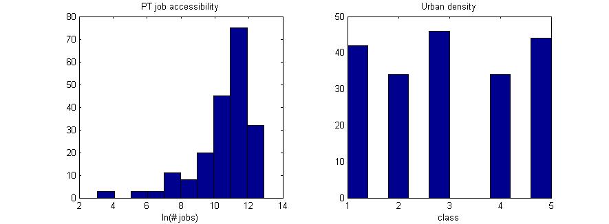
82 82

83 Appendix C: Additional model estimation results This appendix contains model estimation results additional to those included in chapter 4. MNL with all variables Mode Parameter Value SD T-test P Bike ASC -3,95 1,59-2,49 0,01 Travel time -0,16 0,01-14,39 0,00 Delay -0,11 0,02-5,18 0,00 Route 0,23 0,09 2,59 0,01 Attitude 0,80 0,13 6,11 0,00 Habit 0,83 0,07 12,30 0,00 Income 0,19 0,04 4,93 0,00 Infrastructure 0,05 0,10 0,48 0,63 Hindrance -0,29 0,22-1,35 0,18 Lighting -0,33 0,51-0,65 0,52 Surroundings -0,16 0,40-0,41 0,68 Job accessibility 0,00 0,11 0,03 0,97 Gender 0,04 0,16 0,24 0,81 Age 0,00 0,01 0,21 0,83 Car ASC 0, Travel time -0,10 0,02-6,13 0,00 Delay -0,06 0,02-3,99 0,00 Cost -0,27 0,10-2,67 0,01 Job accessibility -0,11 0,13-0,86 0,39 PT ASC -2,95 1,62-1,83 0,07 Travel time -0,10 0,02-5,73 0,00 Delay -0,05 0,02-2,99 0,00 Cost -0,24 0,11-2,22 0,03 Job accessibility 0,14 0,07 1,86 0,06 Urban density -0,11 0,08-1,25 0,21 Walk ASC 0,85 1,91 0,44 0,66 Travel time -0,24 0,05-4,67 0,00 Delay -0,08 0,10-0,76 0,45 Log-likelihood Initial Final ,489 Table C-1: Estimation results for an MNL model with all variables 83

84 Urban density Mode Parameter Value SD T-test P Bike ASC -1,90 0,37-5,11 0,00 Travel time -0,16 0,01-14,51 0,00 Delay -0,11 0,02-5,10 0,00 Route 0,22 0,09 2,49 0,01 Attitude 0,81 0,13 6,34 0,00 Habit 0,82 0,06 12,74 0,00 Income 0,19 0,03 6,11 0,00 Car ASC 0, Travel time -0,10 0,02-6,10 0,00 Delay -0,06 0,02-3,93 0,00 Cost -0,26 0,10-2,63 0,01 PT ASC 0,33 0,28 1,16 0,25 Travel time -0,10 0,02-5,73 0,00 Delay -0,05 0,02-2,96 0,00 Cost -0,24 0,11-2,23 0,03 Urban density -0,25 0,06-4,32 0,00 Walk ASC 2,29 1,09 2,10 0,04 Travel time -0,25 0,05-4,88 0,00 Log-likelihood Initial Final ,491 Table C-2: Estimation results of the full MNL model with urban density instead of PT job accessibility Note that the value of the urban density variable decreases with increasing density (see appendix A) 84

85 Effects coding Income Mode Parameter Value SD T-test P Bike ASC -0,62 0,88-0,71 0,48 Travel time -0,29 0,02-13,08 0,00 Delay -0,19 0,03-6,49 0,00 Route 0,44 0,11 3,87 0,00 Attitude 1,09 0,39 2,75 0,01 Habit 1,39 0,20 6,92 0,00 Income A 1,33 0,31 4,25 0,00 Income B -0,09 0,25-0,34 0,73 Error component Car ASC Travel time -0,21 0,03-7,28 0,00 Delay -0,13 0,02-5,06 0,00 Cost -0,43 0,16-2,69 0,01 Error component 2,71 0,28 9,69 0,00 PT ASC -5,50 1,65-3,32 0,00 Travel time -0,20 0,03-7,31 0,00 Delay -0,07 0,02-2,72 0,01 Cost -0,42 0,16-2,73 0,01 Job accessibility 0,47 0,13 3,56 0,00 Error component 2,97 0,35 8,51 0,00 Walk ASC 1,10 2,05 0,54 0,59 Travel time -0,31 0,09-3,32 0,00 Error component 3,65 1,20 3,05 0,00 Log-likelihood Initial Final ,5 Table C-3: Estimation results of an EC model with income as effects coded variable 85

86 Route Mode Parameter Value SD T-test P Bike ASC -2,29 1,03-2,23 0,03 Travel time -0,28 0,02-13,20 0,00 Delay -0,19 0,03-6,45 0,00 Income 0,37 0,09 4,21 0,00 Attitude 1,05 0,41 2,57 0,01 Habit 1,47 0,19 7,88 0,00 Route A 0,36 0,13 2,87 0,00 Route B 0,18 0,13 1,40 0,16 Error component Car ASC Travel time -0,21 0,03-7,28 0,00 Delay -0,12 0,03-4,64 0,00 Cost -0,42 0,16-2,61 0,01 Error component 2,72 0,28 9,77 0,00 PT ASC -4,92 1,83-2,69 0,01 Travel time -0,21 0,03-7,35 0,00 Delay -0,06 0,03-2,54 0,01 Cost -0,39 0,16-2,48 0,01 Job accessibility 0,42 0,14 2,99 0,00 Error component 2,94 0,38 7,77 0,00 Walk ASC 0,85 1,79 0,47 0,64 Travel time -0,33 0,07-4,48 0,00 Error component 4,23 0,81 5,21 0,00 Log-likelihood Initial Final ,5 Table C-4: Estimation results of an EC model with route impression as effects coded variable 86

87 Age Mode Parameter Value SD T-test P Bike ASC -3,63 1,33-2,73 0,01 Travel time -0,29 0,02-13,29 0,00 Delay -0,19 0,03-6,53 0,00 Route 0,45 0,11 3,93 0,00 Attitude 0,95 0,43 2,23 0,03 Habit 0,95 0,43 2,23 0,03 Income 0,41 0,10 4,27 0,00 Age A 0,27 0,33 0,82 0,41 Age B -0,21 0,29-0,73 0,47 Error component Car ASC Travel time -0,21 0,03-7,36 0,00 Delay -0,13 0,03-5,06 0,00 Cost -0,43 0,17-2,55 0,01 Error component 2,87 0,32 8,90 0,00 PT ASC -6,06 1,67-3,63 0,00 Travel time -0,20 0,03-7,32 0,00 Delay -0,07 0,02-2,70 0,01 Cost -0,44 0,16-2,82 0,00 Job accessibility 0,50 0,13 3,85 0,00 Error component 2,68 0,27 9,88 0,00 Walk ASC 0,08 2,38 0,03 0,97 Travel time -0,30 0,08-3,60 0,00 Error component 3,92 0,85 4,62 0,00 Log-likelihood Initial Final ,499 Table C-5: Estimation results of an EC model with age as effects coded variable 87

88 Appendix D: Priors and levels used for survey optimization Table D-1 lists the priors and levels used in ngene for choice set generation, using the D-efficient design method. There are three choice sets: for short (<4 km), medium (4-7 km) and longer distances (8-12 km). Each choice set has its own set of levels, but uses the same priors. The mode walking was not included in the long choice set, as it would be extremely unattractive. Mode Variable Prior Levels Short Medium Long Bike ASC Travel time -0, Delay -0, Route impression -0, Car ASC Travel time -0, Cost -0,85 0,5 1 1,5 1,5 2 2, Delay -0, PT ASC Travel time -0, Cost -0,80 0,5 1 1,5 1,5 2 2, Delay -0, Walk ASC Travel time -0, Delay -0, Table D-1: Levels and priors used for survey optimization 11 Normalized to zero. 88

89 Appendix E: Survey The following pages are a transcript of the web-based survey developed for this research. Note that the survey is in Dutch, and that all routing and dynamic aspects of the survey cannot be represented in this format. As a result, some texts and images are displayed up to six times, with slight differences, while a respondent would only see one. 89

90 Onderzoek naar vervoerswijzekeuze forenzen Deze vragenlijst is onderdeel van een onderzoek van de Universiteit Twente en Goudappel Coffeng naar de vervoerswijzekeuze van forenzen. De resultaten van het onderzoek zullen worden gebruikt om bestaande vervoersmodellen te verbeteren, met name voor de fiets. Met behulp van deze verbeterde modellen kunnen gemeenten, provincies en het rijk betere beslissingen nemen over, onder andere, de aanleg en het onderhoud van (fiets)infrastructuur. De vragenlijst neemt ongeveer 10 minuten in beslag, en bestaat uit de volgende vijf onderdelen: een recente verplaatsing, enkele keuzescenario s, uw gewoonte en houding met betrekking tot fietsen, faciliteiten en beleid op uw werkplek, en tot slot enkele algemene vragen. Deze vragenlijst is volledig anoniem: u wordt niet gevraagd uw naam of contactgegevens af te geven. Uw antwoorden zijn niet tot u herleidbaar.

91 Bent u werkzaam? nmlkj Ja nmlkj Nee Werkt u op een andere lokatie dan uw woning? Noot: een praktijk, winkel of werkplaats aan huis geldt niet als een andere lokatie. nmlkj Ja, (vrijwel) altijd nmlkj Ja, regelmatig nmlkj Soms nmlkj Nee, (vrijwel) nooit

92 Recente verplaatsing Wat zijn de vier cijfers van de postcode van uw woning? gfedc Weet niet In welke gemeente staat uw woning? Wat zijn de vier cijfers van de postcode van uw werklokatie? Let op: Vul de postcode van het bezoekadres in. Indien u op meerdere lokaties werkt, kies dan de lokatie waar u het vaakst naartoe gaat. gfedc Weet niet In welke gemeente bevindt uw werklokatie zich? Kunt u een schatting geven van de afstand tussen beiden, in kilometers? Noot: Gebruik een punt in plaats van een komma voor decimalen.

93 Alternatieve recente verplaatsing U hebt bij de vorige vraag een relatief lange afstand ingevuld. Dit betekent dat de komende scenario's waarschijnlijk niet aansluiten bij uw situatie. Om toch de vragenlijst in te kunnen vullen, dient u een andere recente verplaatsing in gedachten nemen. Neem een korte recente verplaatsing (korter dan 15km) in gedachten, die u met enige regelmaat maakt, bijvoorbeeld naar een winkelcentrum, familie of vrienden. Wat zijn de vier cijfers van de postcode van uw vertreklokatie? gfedc Weet niet In welke gemeente bevindt de vertreklokatie zich? Wat zijn de vier cijfers van de postcode van uw bestemming? gfedc Weet niet In welke gemeente bevindt uw bestemming zich? Kunt u een schatting geven van de afstand tussen beiden, in kilometers? Noot: Gebruik een punt in plaats van een komma voor decimalen. Stelt u zich gedurende de rest van de vragenlijst voor, dat u deze verplaatsing dagelijks naar uw werk maakt.

94 Recente verplaatsing Hoe heeft u de afstand, of het grootste deel daarvan, afgelegd? nmlkj Met de auto nmlkj Met de trein nmlkj Met ander openbaar vervoer (bus, tram of metro) nmlkj Met de fiets nmlkj Met de bromfiets of scooter nmlkj Lopend nmlkj Ander vervoersmiddel Welk ander vervoersmiddel heeft u gebruikt? Kunt u een schatting geven van de reistijd, van deur tot deur, in minuten? Hoeveel minuten van deze tijd zou u aanmerken als vertraging? In andere woorden: hoeveel minuten sneller zou u in het best mogelijke geval zijn geweest? Heeft u de beschikking over een auto voor woon-werkverkeer? nmlkj Ja nmlkj Soms nmlkj Nee

95 Keuzescenario's U krijgt nu negen keer een aantal alternatieve vervoerswijzen te zien. U kunt steeds kiezen of u in die situatie met de auto, het openbaar vervoer (bus, tram en/of metro), fietsend of lopend naar uw werk zou gaan. De vervoerswijzen kunt u vergelijken op basis van reistijd, vertraging, de kosten en (voor de fiets) een routeimpressie. U krijgt nu negen keer een aantal alternatieve vervoerswijzen te zien. U kunt steeds kiezen of u in die situatie met de auto, het openbaar vervoer (bus, tram en/of metro) of fietsend naar uw werk zou gaan. De vervoerswijzen kunt u vergelijken op basis van reistijd, vertraging, de kosten en (voor de fiets) een route-impressie. U krijgt nu negen keer een aantal alternatieve vervoerswijzen te zien. U kunt steeds kiezen of u in die situatie met het openbaar vervoer (bus, tram en/of metro) of fietsend naar uw werk zou gaan. De vervoerswijzen kunt u vergelijken op basis van reistijd, vertraging, de kosten en (voor de fiets) een route-impressie. U krijgt nu negen keer een aantal alternatieve vervoerswijzen te zien. U kunt steeds kiezen of u in die situatie met het openbaar vervoer (bus, tram en/of metro), fietsend of lopend naar uw werk zou gaan. De vervoerswijzen kunt u vergelijken op basis van reistijd, vertraging, de kosten en (voor de fiets) een route-impressie. Voorbeeldscenario

96

97

98

99 Elk scenario bevat een fietsroute-impressie, gegeven doormiddel van een foto. U moet zich voorstellen dat die foto representatief is voor die route. Naast die in het voorbeeld, kunnen de volgende impressies kunnen worden getoond:

100 Drukke klinkerweg met parkeerhavens, maar met duidelijke fietsstroken Zeer drukke weg met parkeerhavens, zonder enige fietsvoorzieningen Zou u in werklijkheid geen van de getoonde vervoerswijzen kiezen, maar bijvoorbeeld vanuit huis gaan werken, kunt u dit onderaan de scenario's aangeven.

101 Scenario 1 Welk vervoersmiddel zou u kiezen om naar uw werk te gaan? nmlkj Auto nmlkj Openbaar vervoer nmlkj Fiets nmlkj Lopen

102 Welk vervoersmiddel zou u kiezen om naar uw werk te gaan? nmlkj Auto nmlkj Openbaar vervoer nmlkj Fiets nmlkj Lopen

103 Welk vervoersmiddel zou u kiezen om naar uw werk te gaan? nmlkj Auto nmlkj Openbaar vervoer nmlkj Fiets

104 Welk vervoersmiddel zou u kiezen om naar uw werk te gaan? nmlkj Openbaar vervoer nmlkj Fiets nmlkj Lopen

105 Welk vervoersmiddel zou u kiezen om naar uw werk te gaan? nmlkj Openbaar vervoer nmlkj Fiets nmlkj Lopen

106 Welk vervoersmiddel zou u kiezen om naar uw werk te gaan? nmlkj Openbaar vervoer nmlkj Fiets gfedc Ik zou, gegeven deze opties, afzien van de verplaatsing Kunt u aangeven waarom?

107 Scenario 2 Welk vervoersmiddel zou u kiezen om naar uw werk te gaan? nmlkj Auto nmlkj Openbaar vervoer nmlkj Fiets nmlkj Lopen

108 Welk vervoersmiddel zou u kiezen om naar uw werk te gaan? nmlkj Auto nmlkj Openbaar vervoer nmlkj Fiets nmlkj Lopen

109 Welk vervoersmiddel zou u kiezen om naar uw werk te gaan? nmlkj Auto nmlkj Openbaar vervoer nmlkj Fiets

110 Welk vervoersmiddel zou u kiezen om naar uw werk te gaan? nmlkj Openbaar vervoer nmlkj Fiets nmlkj Lopen

111 Welk vervoersmiddel zou u kiezen om naar uw werk te gaan? nmlkj Openbaar vervoer nmlkj Fiets nmlkj Lopen

112 Welk vervoersmiddel zou u kiezen om naar uw werk te gaan? nmlkj Openbaar vervoer nmlkj Fiets gfedc Ik zou, gegeven deze opties, afzien van de verplaatsing Kunt u aangeven waarom?

113 Scenario 3 Welk vervoersmiddel zou u kiezen om naar uw werk te gaan? nmlkj Auto nmlkj Openbaar vervoer nmlkj Fiets nmlkj Lopen

114 Welk vervoersmiddel zou u kiezen om naar uw werk te gaan? nmlkj Auto nmlkj Openbaar vervoer nmlkj Fiets nmlkj Lopen

115 Welk vervoersmiddel zou u kiezen om naar uw werk te gaan? nmlkj Auto nmlkj Openbaar vervoer nmlkj Fiets

116 Welk vervoersmiddel zou u kiezen om naar uw werk te gaan? nmlkj Openbaar vervoer nmlkj Fiets nmlkj Lopen

117 Welk vervoersmiddel zou u kiezen om naar uw werk te gaan? nmlkj Openbaar vervoer nmlkj Fiets nmlkj Lopen

118 Welk vervoersmiddel zou u kiezen om naar uw werk te gaan? nmlkj Openbaar vervoer nmlkj Fiets gfedc Ik zou, gegeven deze opties, afzien van de verplaatsing Kunt u aangeven waarom?

119 Scenario 4 Welk vervoersmiddel zou u kiezen om naar uw werk te gaan? nmlkj Auto nmlkj Openbaar vervoer nmlkj Fiets nmlkj Lopen

120 Welk vervoersmiddel zou u kiezen om naar uw werk te gaan? nmlkj Auto nmlkj Openbaar vervoer nmlkj Fiets nmlkj Lopen

121 Welk vervoersmiddel zou u kiezen om naar uw werk te gaan? nmlkj Auto nmlkj Openbaar vervoer nmlkj Fiets

122 Welk vervoersmiddel zou u kiezen om naar uw werk te gaan? nmlkj Openbaar vervoer nmlkj Fiets nmlkj Lopen

123 Welk vervoersmiddel zou u kiezen om naar uw werk te gaan? nmlkj Openbaar vervoer nmlkj Fiets nmlkj Lopen

124 Welk vervoersmiddel zou u kiezen om naar uw werk te gaan? nmlkj Openbaar vervoer nmlkj Fiets gfedc Ik zou, gegeven deze opties, afzien van de verplaatsing Kunt u aangeven waarom?

125 Scenario 5 Welk vervoersmiddel zou u kiezen om naar uw werk te gaan? nmlkj Auto nmlkj Openbaar vervoer nmlkj Fiets nmlkj Lopen

126 Welk vervoersmiddel zou u kiezen om naar uw werk te gaan? nmlkj Auto nmlkj Openbaar vervoer nmlkj Fiets nmlkj Lopen

127 Welk vervoersmiddel zou u kiezen om naar uw werk te gaan? nmlkj Auto nmlkj Openbaar vervoer nmlkj Fiets

128 Welk vervoersmiddel zou u kiezen om naar uw werk te gaan? nmlkj Openbaar vervoer nmlkj Fiets nmlkj Lopen

129 Welk vervoersmiddel zou u kiezen om naar uw werk te gaan? nmlkj Openbaar vervoer nmlkj Fiets nmlkj Lopen

130 Welk vervoersmiddel zou u kiezen om naar uw werk te gaan? nmlkj Openbaar vervoer nmlkj Fiets gfedc Ik zou, gegeven deze opties, afzien van de verplaatsing Kunt u aangeven waarom?

131 Scenario 6 Welk vervoersmiddel zou u kiezen om naar uw werk te gaan? nmlkj Auto nmlkj Openbaar vervoer nmlkj Fiets nmlkj Lopen

132 Welk vervoersmiddel zou u kiezen om naar uw werk te gaan? nmlkj Auto nmlkj Openbaar vervoer nmlkj Fiets nmlkj Lopen

133 Welk vervoersmiddel zou u kiezen om naar uw werk te gaan? nmlkj Auto nmlkj Openbaar vervoer nmlkj Fiets

134 Welk vervoersmiddel zou u kiezen om naar uw werk te gaan? nmlkj Openbaar vervoer nmlkj Fiets nmlkj Lopen

135 Welk vervoersmiddel zou u kiezen om naar uw werk te gaan? nmlkj Openbaar vervoer nmlkj Fiets nmlkj Lopen

136 Welk vervoersmiddel zou u kiezen om naar uw werk te gaan? nmlkj Openbaar vervoer nmlkj Fiets gfedc Ik zou, gegeven deze opties, afzien van de verplaatsing Kunt u aangeven waarom?

137 Scenario 7 Welk vervoersmiddel zou u kiezen om naar uw werk te gaan? nmlkj Auto nmlkj Openbaar vervoer nmlkj Fiets nmlkj Lopen

138 Welk vervoersmiddel zou u kiezen om naar uw werk te gaan? nmlkj Auto nmlkj Openbaar vervoer nmlkj Fiets nmlkj Lopen

139 Welk vervoersmiddel zou u kiezen om naar uw werk te gaan? nmlkj Auto nmlkj Openbaar vervoer nmlkj Fiets

140 Welk vervoersmiddel zou u kiezen om naar uw werk te gaan? nmlkj Openbaar vervoer nmlkj Fiets nmlkj Lopen

141 Welk vervoersmiddel zou u kiezen om naar uw werk te gaan? nmlkj Openbaar vervoer nmlkj Fiets nmlkj Lopen

142 Welk vervoersmiddel zou u kiezen om naar uw werk te gaan? nmlkj Openbaar vervoer nmlkj Fiets gfedc Ik zou, gegeven deze opties, afzien van de verplaatsing Kunt u aangeven waarom?

143 Scenario 8 Welk vervoersmiddel zou u kiezen om naar uw werk te gaan? nmlkj Auto nmlkj Openbaar vervoer nmlkj Fiets nmlkj Lopen

144 Welk vervoersmiddel zou u kiezen om naar uw werk te gaan? nmlkj Auto nmlkj Openbaar vervoer nmlkj Fiets nmlkj Lopen

145 Welk vervoersmiddel zou u kiezen om naar uw werk te gaan? nmlkj Auto nmlkj Openbaar vervoer nmlkj Fiets

146 Welk vervoersmiddel zou u kiezen om naar uw werk te gaan? nmlkj Openbaar vervoer nmlkj Fiets nmlkj Lopen

147 Welk vervoersmiddel zou u kiezen om naar uw werk te gaan? nmlkj Openbaar vervoer nmlkj Fiets nmlkj Lopen

148 Welk vervoersmiddel zou u kiezen om naar uw werk te gaan? nmlkj Openbaar vervoer nmlkj Fiets gfedc Ik zou, gegeven deze opties, afzien van de verplaatsing Kunt u aangeven waarom?

149 Scenario 9 Welk vervoersmiddel zou u kiezen om naar uw werk te gaan? nmlkj Auto nmlkj Openbaar vervoer nmlkj Fiets nmlkj Lopen

150 Welk vervoersmiddel zou u kiezen om naar uw werk te gaan? nmlkj Auto nmlkj Openbaar vervoer nmlkj Fiets nmlkj Lopen

151 Welk vervoersmiddel zou u kiezen om naar uw werk te gaan? nmlkj Auto nmlkj Openbaar vervoer nmlkj Fiets

152 Welk vervoersmiddel zou u kiezen om naar uw werk te gaan? nmlkj Openbaar vervoer nmlkj Fiets nmlkj Lopen

153 Welk vervoersmiddel zou u kiezen om naar uw werk te gaan? nmlkj Openbaar vervoer nmlkj Fiets nmlkj Lopen