AN ABSTRACT OF THE THESIS OF

Transcription

1 AN ABSTRACT OF THE THESIS OF Justin Hovland for the degree of Master of Science in Mechanical Engineering presented on April 26, Title: Predicting Deep Water Breaking Wave Severity Abstract approved: Robert K. Paasch Ocean Wave Energy Converters (WECs) operating on the water surface are subject to storms and other extreme events. In particular, high and steep waves, especially breaking waves, are likely the most dangerous to WECs. A method for quantifying the breaking severity of waves is presented and applied to wave data from Coastal Data Information Program station 139. The data are wave height and length statistics found by conducting a zero-crossing analysis of time-series wave elevation records. Data from the top ten most severe storms in the data set were analyzed. In order to estimate the breaking severity, two different steepness-based breaking criteria were utilized, one being the steepness where waves begin to show a tendency to break, the other the steepness above which waves are expected to break. Breaking severity is assigned as a fuzzy membership function between the two conditions. The distribution of breaking severity is found to be exponential. It is shown that the highest waves are not necessarily the most dangerous. Even so, waves expected to be breaking are observed being up to 17 meters tall at station 139.

2 Copyright by Justin Hovland April 26, 2010 All Rights Reserved

3 Predicting Deep Water Breaking Wave Severity by Justin Hovland A THESIS submitted to Oregon State University in partial fulfillment of the requirements for the degree of Master of Science Presented April 26, 2010 Commencement June 2010

4 Master of Science thesis of Justin Hovland presented on April 26, APPROVED: Major Professor, representing Mechanical Engineering Head of the School of Mechanical, Industrial and Manufacturing Engineering Dean of the Graduate School I understand that my thesis will become part of the permanent collection of Oregon State University libraries. My signature below authorizes release of my thesis to any reader upon request. Justin Hovland, Author

5 ACKNOWLEDGEMENTS I would like to thank my parents for always supporting me in my pursuits and for always encouraging me to do my best and follow things through. From answering all of my questions as a child, being interested and involved in my hobbies growing up, and always wanting to hear about what I m doing, they have been paving the road in front of me as I ve bumbled myself along. I d also like to thank Dr. Robert Paasch and Dr. Irem Tumer for bringing me into the OSU community and letting me explore this interesting topic so freely. My fellow students - Adam, Pukha, Kelley and Steve - have all helped me greatly by reviewing my work, hashing things out on the chalk board, and listening to my rants. Finally, I thank all of my friends, particularly the Finer Foods Club, for helping me stay sort of sane through good conversation and good food, for exploring this beautiful state with me, and for making my life here so much richer.

6 This material is based upon work supported by the Department of Energy under Award Number DE-FG36-08GO Disclaimer: This report was prepared as an account of work sponsored by an agency of the United States Government. Neither the United States Government nor any agency thereof, nor any of their employees, makes any warranty, expressed or implied, or assumes any legal liability or responsibility for the accuracy, completeness, or usefulness of any information, apparatus, product, or process disclosed, or represents that its use would not infringe privately owned rights. Reference herein to any specific commercial product, process, or service by trade name, trademark, manufacturer, or otherwise does not necessarily constitute or imply its endorsement, recommendation, or favoring by the United States Government or any agency thereof. The views and opinions of the authors expressed herein do not necessarily state or reflect those of the United States Government or any agency thereof.

7 TABLE OF CONTENTS Page 1. INTRODUCTION Motivation: Ocean Power and Sustainability Possible Negative Effects History of the Research History of the Industry Contributions From OSU and the NNMREC The Issue of Survivability WAVE GROWTH, MODULATION, AND INSTABILITY Creation, Propagation and Dispersion The Modulation (B-F) Instability Non-linear Resonant 4-wave interactions DEEP WATER WAVE BREAKING Kinematic Criteria Dynamic Criteria Geometric Criteria WAVE STATISTICS AND DISTRIBUTIONS The Wave Spectrum The Rayleigh Distribution The Joint Distribution and Breaking Probability WAVE DATA AND HANDLING Data Availability from NDBC and CDIP Spectral Files Parameter Files Time-Series Files Erroneous Data and Gaps STORM FINDING AND CATALOGING Storm Definition and Finding...39

8 TABLE OF CONTENTS (Continued) Page 6.2 Recorded Storms Predicting Storm Return A METHOD TO DESCRIBE BREAKING SEVERITY Dual Breaking Criteria and the Breaking Severity Time-series Data Analysis and Joint Distributions The Breaking Severity Factor Distribution Other Methods of Obtaining the Joint Distribution DISCUSSION AND CONCLUSIONS Usefulness of the Breaking Severity Parameter Implications for WECs Possible Future Directions...62 REFERENCES...64

9 Figure LIST OF FIGURES Page 1. Plan view of the three geometrical WEC classes Some sea tested WECs. From the upper left: LIMPET, Wave Dragon, Power Buoy, and Pelamis Geometrical wave properties Deep water wave speed considering effects of surface tension Water particle velocity vectors and particle paths Example of wave superposition and spectral transformation Left: a single spectra during the height of a storm. Right: spectra every 5 hours from the beginning (blue) to the end (red) of a storm Examples of directional spectra generated by CDIP. Left: peak of Storm 1. Right: end of Storm Wave envelope function for a real wave profile Distribution of wave heights during Storm Examples of Longuet-Higgins joint distribution. Left: v = 0.25, Right: v = Lat-long map showing the distribution and availability of wave data on the US west coast Example of a spectral file from CDIP Example of a parameter file from CDIP Example of a time-series file from CDIP Examples of erroneous data. Left: a spike in a time-series. Right: two erroneous spectra during a storm Rate-of-change quality control of significant wave height records Storms on the significant height record for CDIP station Significant height plots of the top ten storms at CDIP station 139, ranked by significant height Top ten storms at CDIP station Fuzzy membership function of breaking probability by steepness Joint distribution of wave height and period for the top ten storms at CDIP station 139 (continued) Joint distribution of wave height and period during calm seas...51

10 Figure LIST OF FIGURES (Continued) Page 24. Joint distribution during three segments of Storm Joint distribution during three segments of Storm Breaking severity distribution for the top ten storms at station 139 (continued) Spectral simulation of the joint distribution during Storm 1. Left: 64 frequency bins. Right: 512 frequency bins...58

11 LIST OF TABLES Table Page 1. Listing of storms identified at CDIP Station Breaking severity distribution parameters for the top ten storms...57

12 LIST OF ACRONYMS AWS CDIP CPT EMEC IEC LIMPET NDBC NNMREC NOAA NWS OPT OSU OWC UW WEC WESRF Archimedes Wave Swing Coastal Data Information Program Columbia Power Technologies European Marine Energy Centre International Electrotechnical Commission Land Installed Marine Power Energy Transmitter National Data Buoy Center Northwest National Marine Renewable Energy Center National Oceanic and Atmospheric Administration National Weather Service Ocean Power Technologies Oregon State University Oscillating Water Column University of Washington Wave Energy Converter Wallace Energy Systems and Renewable Facility

13 LIST OF VARIABLES A Wave amplitude (m) B Breaking severity factor (m) b Normalized lower breaking threshold c Wave speed [celerity] (m/s) f Wave frequency (Hz) F Variance density of the wave spectrum (m 2 /Hz) f(s) Breaking probability based on steepness g Acceleration of gravity (m/s 2 ) h Water depth (m) H Wave height (m) H m0 Spectrally derived significant wave height (m) H rms Root mean square wave height (m) H S Significant wave height (m) k Wave number (1/m) L Wave length (m) m n N th moment of the wave spectrum R Amplitude parameter for Longuet-Higgins joint distribution S Wave steepness S N Normalized wave steepness T Wave Period (s) T P v v J Z Peak spectral period (s) Spectral width parameter Power spectral width parameter Period parameter for Longuet-Higgins joint distribution ρ Water density (kg/m 3 ) σ Radian wave frequency (rad/s) σ 0 τ Radian Carrier wave frequency (rad/s) Surface tension (N/m)

14 Predicting Deep Water Breaking Wave Severity 1. INTRODUCTION This thesis has been written for three reasons: to organize my own thoughts, to help inform other students and researchers, and to convince my committee to graduate me. The purpose of this document is to help you understand my thought process and form an idea of my thesis statement in your mind. My thesis statement, by the way, is: Wave breaking severity may be statistically linked to the distribution of wave steepness. If you are already familiar with waves and wave energy, you may be most interested to read Sections 6-8 which present a listing of storms off the Oregon coasts and the introduction of a breaking severity parameter intended to predict breaking waves during a given storm. My conclusions also identify further questions such as how my parameter might be related to observed slamming wave geometries, how the presence of a structure could alter the slamming characteristics, and how a series of slamming loads might be used to model the behavior of wave energy converters. That said, those sections do depend on the material presented in Sections 1-5. In the next sixty-so pages I will try to explain why I decided to study breaking waves, the tools I have found with which to do so, and what I have added to the field. I will start with an introduction to some of the progress made in wave energy research and industry, and explain where I fit into it. From there on out I will focus on waves themselves. I will talk about how waves grow and interact in Section 2, then how and when they break in Section 3. Some fundamental statistical methods of describing waves will be introduced in Section 4; these are central to understanding archived wave data. In Section 5, I will discuss the available sources of wave data as well as the data I used for my investigation. Storms and how to isolate them in the wave records will be the subject of Section 6. In Section 7 I will explain how I analyzed the waves during particular storms, and how I defined a wave breaking severity. This section represents my own original work and my primary contribution to the field. Finally, Section 8 closes with a discussion of some implications and future directions stemming from my work, tying the material back to wave energy devices and survivability.

15 2 1.1 Motivation: Ocean Power and Sustainability I took a course on renewable energy during my undergraduate program at the University of Wyoming, where two essential points became clear: our energy supplies should be both sustainable and diverse. Sustainability means being able to carry on indefinitely without adverse effect to the environment. Diverse means we should not put all of our eggs in one basket. Currently, some major potential sustainable power sources include solar (thermal and photo-voltaic), wind, geothermal, wave, and tidal power. It would be prudent if we could develop all of these technologies in order to bring our dependence on fossil fuels to an end. Even if the techno-dream of achieving sustained nuclear fusion is realized, it should still be only a part of the bigger picture. So whether we can include wave energy in our portfolio or not really depends on how much power is out there and if we have enough ingenuity and ability to take advantage of it. So far the power levels are looking pretty good, but we have yet to demonstrate the full-scale utilization of it, and have a good deal of work to do to get to that point. The power available from the sea has been fairly well established, but it fluctuates depending on a variety of time and length scales. A good starting point for understanding the spatial and temporal distribution of wave energy is Chapter 4 of Ocean Wave Energy by Cruz [1]. For the Pacific Northwest, the annual average power level approaches 40 kw/m, while summer and winter values are around kw/m and kw/m, respectively. During a storm, the power can exceed 1000 kw/m. The unit here describes power available per meter length along a wave crest. For example, if 40 kw/m of wave power was incident over the entire Oregon coast, which I will take as 500 km long, then 20 GW (20,000,000 kw) of power would be available over the entire coast at that time. Note that these power levels are for offshore waters and carry the implication that devices which utilize the stated power will be at least 2 or 3 miles offshore. 1.2 Possible Negative Effects Even if we become capable of extracting as much energy as we wish from the waves, the development of power facilities must not have significant adverse environmental or social effects. Possible environmental effects include changing coastal

16 3 erosion patterns, harming migrating whales, disrupting marine life, and polluting the water. Some social effects include disrupting transportation as well as the fishing community and industry. These issues must be considered in concert with the purely technical question of power production, and this is currently being done in the United States as will be discussed more below in Section 1.5 on OSU and the NNMREC. 1.3 History of the Research The power of the sea has long impressed the human race and no doubt some people have dreamt of ways to put it to use over time. This dream took on a more serious nature at least by the turn of the 20 th century, as a 1898 patent by P. Wright for a wave motor indicates [2]. It appears that wave power has had three forays into the public eye, the first between the two World Wars, the second in the 70s, and the third presently although it may also be viewed as a resurgence of the second. A good review of the principles of wave energy extraction was recently published by Falnes [3], and a more comprehensive recent review of wave energy technology is given by Drew et al. [4] Early Interest: Pre-WWII In the 1920s and 30s a sizable portion of the scientific community (including Nikola Tesla, who helped create our electric capacity) regarded renewable energy as the only reasonable way to power our society in the long term. The idea of nuclear power was at this time met with some skepticism, and was not generally regarded as being an effective possibility. Instead, they envisioned cities powered by the sun and the waves. After World War I numerous patents on wave power devices began to be filed [5]. A couple of articles published in Modern Mechanix in the 30s described designs for inertial wave energy buoys [6], generating public knowledge and interest the subject. However, after World War II and the advent of nuclear power, the visions of a sustainable future seem to have been replaced by visions of plastic everything and the convenient home appliance. Coal and oil were established sources of expandable energy that quietly grew to staggering proportions to feed the multiplying number of energy consuming devices that now permeate our everyday life. Nuclear fission, the miracle of the new era, was positioned as the only future source of energy we would need, though even now it only

17 4 accounts for about 6% of our energy supply (while fossil fuels account for some 81% of it) [7]. It wasn t until the oil crisis of 1973 that renewable energy was put back into the spotlight. Then, over about a decade, a number of European academics promoted wave energy and provided much of the theoretical background on wave energy conversion Beginning of Modern Interest The first researcher to seriously investigate wave energy converters (WECs) was Stephen Salter. He developed the infamous duck (or Salter Cam) which was shown in 1974 to be capable of extracting virtually all of the energy out of a wavetrain [5]. Further studies establishing the potential of Salter s Cam were authored by Mynett in 1979 [8] and by Greenhow in 1981 [9]. An interesting account of the research that took place in Edinburgh during this period is given in a short book by Ross [10]. It is worth noting here that this research program was effectively (and actively) killed by the nuclear industry in the UK using forms of political manipulation, as described (cautiously) by Salter in his chapter of Ocean Wave Energy by Cruz [1]. David Evans developed much of the theoretical background behind wave power absorption and efficiency, much of which is presented in a 1976 publication [11]. Evans showed that devices with one mode of oscillation (such as heave) can extract up to 50% of the incident wave energy, while a device operating in two modes can theoretically extract 100%. At the same time, Mei independently obtained the same results [12]. Newman also presented material on wave-structure interaction that overlaps with much of the work of both Evans and Mei [13]. Based on these initial findings, Evans et al. published some theory and experiments in 1979 on a simple submerged cylinder device (the Bristol Cylinder), showing it to be capable of extracting all of the energy in a wave [14]. Even so, if you investigate these works, you will find that the physical conditions necessary to achieve these theoretical maxima (e.g. device/wavelength ratio and amplitude response ratio) may be difficult to practically construct and operate. In 1975, Budal and Falnes published an article describing a buoy-type device, aiming at a manageable size instead of perfect absorption [15]. At the same time, but in America, McCormick was also investigating point absorber buoys [16]. Because they

18 5 operate in only one mode of motion, buoys cannot extract more than half of the incident energy. Regardless, this has become one of the most popular general architectures for developers. In 1979, Haren and Mei published a study on hinged rafts used to extract wave energy [17], as did Newman [18]. In these designs, the length of the device is oriented perpendicular to the wave crests, such that the passing of the waves causes the rafts to articulate. The power absorption characteristics of these devices (attenuators) carries some ambiguity. I have seen them claimed to be capable of perfect absorption, but the rear section has to work just as hard as the front. To my knowledge, perfect absorption by an attenuator has not been demonstrated in a laboratory setting Some Established Concepts Multiple classification systems for WECs have been used over time, some describing the particular operating mode of the device or the era in which it originated. However, the simplest and most clear division of concepts seems to be the geometrical description which classifies a device as one of three things: a terminator, attenuator, or point absorber. Figure 1 shows the basic geometry of each of these three device classes in relation to the oncoming waves from plan view. The horizontal lines represent the wave crests and the weight of each line represents the energy content along the crest. Incoming Waves a) Terminator b) Attenuator c) Point Absorber Figure 1. Plan view of the three geometrical WEC classes

19 6 A terminator is generally oriented parallel to the wave crests. They are theoretically capable of extracting all of the incident wave energy, as indicated by the lower energy waves (lighter lines) behind the terminator device depicted in Figure 1. Examples of such terminators that have been studied include Salter s Cam and the Bristol Cylinder. A word of caution here: the maximum theoretical efficiency of a terminator depends on its mode of operation. The Cam and Cylinder operate in two modes (heave and surge) and do not generate radiated waves, thus they are capable of extracting all of the incident energy under the proper conditions. However, if a terminator device is made to operate in only one mode of motion, such as heaving, then it will only be able to extract a maximum of half of the incident wave energy [11]. A long bank of oscillating water columns (OWCs) could be modeled in this way, though to my knowledge this has not been explicitly confirmed. An attenuator is generally oriented perpendicular to the wave crests and is meant to drain energy out of the wave as it progresses along the body. These may take the form of articulated raft sections (such as the Pelamis device), or a flexible structure pumping a fluid. As mentioned above, discussing the efficiency of such devices is difficult because the wave/structure interaction is spread out along the direction of wave propagation. In thinking about modes of oscillation and wave radiation, it seems like a hinged raft system would generate waves radiating away from the sides of the device, limiting the energy absorption potential. However, as wave energy is absorbed by the device, more energy will diffract in toward the device, thus increasing the incident energy. I have not seen the interplay of these two characteristics clearly elucidated, and so a general description of attenuator efficiency and performance seems to be left wanting. Point absorbers are small in both dimensions with respect to the wavelength. As they oscillate they create a circular radiated wave pattern so that radiated waves traveling perpendicular to the incident waves are generated, therefore they cannot absorb all of the energy in the incident waves. However, if a point absorber is made to heave with an amplitude greater than that of the incoming waves, it can absorb energy out of a length of wave crest wider than its own diameter. In fact, regardless of the device diameter, it can theoretically extract the energy out of a crest width of L/2π, where L is the incident

20 7 wavelength, if the heave amplitude is large enough [11]. This makes point absorbers seem attractive because the same amount of energy could be extracted from a wave front with smaller, less expensive structures. Now, as noted by Evans, there will be a limit to how large the heave amplitude can be before the system becomes physically unrealistic (when linearity or other physics are violated). I d also like to note here that a narrow OWC (oscillating water column) could be modeled as a point absorber. A device class which does not seem to fit into the above architecture is the overtopping device. For it, waves flow up a ramp and fall into an elevated basin, and the water flows through a low pressure turbine back to the sea. This could be thought of as a kind of terminator, but it does not react directly against the waves and likely reflects most of the incident wave energy. I have not seen the efficiency of such devices derived Current Research Trends Current research trends (judging by publication titles) seem to focus on resource assessment, arrays of WECs, and control strategies. Literature on the wave energy resource has recently been published for various locations around Europe and the United States. For the US, I am currently aware of resource description efforts for the Southeast [19], California [20], and the Pacific Northwest [21]. Earlier wave resource estimates were typically made using significant wave height and period data, while today most estimates utilize the more descriptive energy spectrum (discussed more in Section 4). Researchers from OSU have made contributions to this end, which will be discussed in Section 1.5. I am admittedly less aware about the details of the research on WEC arrays and control strategies, suffice to say that both efforts seem to generally assume that the WEC is a buoy. Arrays of buoys were studied as early as 1982 by Falnes and Budal who considered rows of heaving point absorbers and their interference characteristics [22]. In 2009, a study of triangular arrays of buoys was published, with some attention given to the mooring schemes needed to make the array behave as desired [23]. A control strategy that has received much attention over the years is latching control. If the natural frequency of the WEC is higher than that of the waves, the motion of the device may be

21 8 constrained, or latched, at the peak or trough of a wave, and released at the appropriate times to produce as large a displacement as possible. Such schemes have been applied to buoys with favorable results, as described by Falnes [24]. While latching control has been primarily investigated with respect to buoys, the principle may still be applicable to many different WEC architectures, though the method of implementation may differ. 1.4 History of the Industry Many small companies have sprouted up with WEC designs arbitrarily claimed to be the best solution to the problem. I do not intend to focus on what companies have done what, but rather will give a short description of what large-scale testing has been conducted to date. A more detailed discussion of LIMPET, Pelamis, AWS, and Wave Dragon is given in the text by Cruz [1]. Some representative pictures of four of the devices discussed below are shown in Figure Large Scale Testing The first and longest running testing was done with the LIMPET (Land Installed Marine Power Energy Transmitter) device. It is an OWC (Oscillating Water Column) and is installed on the Isle of Islay in Scotland, operated Wavegen of Voith Hydro. The installation has housed more than one device, with the current one having been in place since 2000 and is running today with grid connection. It has a nameplate capacity of 500 kw and a sample years average pneumatic power was 112 kw [1]. It is unclear to me exactly how this related to the actual generated electric power (i.e. if this number account for turbine/generator efficiency). Some other OWC plants have been developed, including the European Pico plant (rated 400 kw) and the Japanese Mighty Whale floating OWC. It is typical for OWC to be shoreline devices, making them easier to install and test, but limiting the available real estate and power. The Archimedes Wave Swing (AWS) is a submerged buoy with an outer float which is pushed down by the passing waves. Some full scale testing was carried out in the early 2000s using a 2 MW rated device with a direct drive linear electric generator. Average power levels during testing seem to be around 25 kw, while they hope to achieve kw in future tests [1].

22 9 wavegen.co.uk wavedragon.net oceanpowertechnologies.com pelamiswave.com Figure 2. Some sea tested WECs. From the upper left: LIMPET, Wave Dragon, Power Buoy, and Pelamis The Pelamis device is probably the most developed and tested sea-faring WEC to date. It is an attenuator made of four articulating pontoon structures with an overall length of about 150 m. It uses hydraulic power take-off and is rated for 750 kw. Sea trials have been conducted in 2004 and 2007 (in the summer). The RMS absorbed and generated power during the 2007 test was 182 and 102 kw respectively [1]. A couple of different buoy devices have been tested, including the OPT (Ocean Power Technologies) Power Buoy and the Finavera Aquabuoy. OPT has tested a 40 kw rated hydraulic buoy in several locations, including Spain, New Jersey, and Hawaii. I have not seen published results of these tests. Finavera deployed a buoy north of Newport, Oregon for about 6 weeks in September Unfortunately, it suffered from a failure and sank (but was recovered later). I have not found data on the test performance. Finally, an overtopping device called the Wave Dragon has been tested at 1:4.5 scale in an inland sea in Denmark since This device has reflector arms meant to focus the wave energy into the basin. While this is not a full-scale device, the length of sea testing is impressive. The device is claimed as being 18% efficient, but this number seems to be an extrapolated expectation, not from actual produced power.

23 The Visible Horizon: Future Testing The European Marine Energy Center (EMEC) has established a testing facility for WECs as well as tidal devices. Pelamis tested there in their earlier 2004 test, and a terminator device dubbed the Oyster is being tested there at the time of this writing. The Oyster is a shallow water device that is similar to a flap-type wave generator, and is actually solidly attached to the seabed. OPT is scheduled to deploy a Power Buoy there in Finally, a Pelamis device is to be deployed there also in OPT is also scheduled to deploy a 150 kw rated Power Buoy off the coast of Reedsport, OR in the summer of Over the next couple years they plan to deploy up to ten buoys in an array. This will mark the first WEC array testing conducted thus far. 1.5 Contributions From OSU and the NNMREC Recent interest in wave energy at OSU began around 1998 with Dr. Annette von Jouanne and Dr. Alan Wallace. The work initiated by Dr. von Jouanne has thus far culminated in OSU-based device development, the formation of an industrial partner, and the birth of the Northwest National Marine Renewable Energy Center (NNMREC). The group that originally started working on wave energy research at OSU is now associated with the Wallace Energy Systems and Renewable Facility (WESRF). They were primarily electrical engineers and were interested in direct-drive electric generators as the power take-off for a WEC. For testing different designs they installed a linear test bed which is meant to replicate the wave induced forces on a power take-off system operating in a single mode of motion (linear). This machine has the distinction of being the largest linear test bed in the nation. The group also evaluated 18 direct-drive power take-off designs and tested five of them on the linear test bed. By 2007, they had designed and built their first large buoy, dubbed the SeaBeav 1, which was tested near Newport as reported by Elwood et al. [25]. Its outer float was just under 2 m in diameter. By this time, several students from WESRF came together to form Columbia Power Technologies (CPT), a company focused on WEC design and testing. Over the next year CPT worked with WESRF to design and build a second-generation buoy, initially called the BlueRay, but now recognized as the L10 (Linear, 10 kw). The float on the L10 was flatter than SeaBeav s, and was about 3 m in diameter. This prototype

24 11 was tested at sea in the summer of Currently, OSU students are not directly involved with the device development. CPT has recently been testing scale models of a newer buoy that utilizes a rotary direct-drive electric generator. OSU students have also been working on describing the wave energy resource in the Pacific Northwest. In 2003, Heng Zhang conducted an analysis of significant height and period data from 4 measurement buoys off the Oregon coast and reported the monthly average power at each station [26]. More recently, my friend and colleague Pukha Lenee-Blum has been working on a more comprehensive characterization of the resource utilizing spectral records from ten different sites ranging from N. California to Washington [21]. His analysis gives us a view of how parameters like directionality and narrow-bandedness vary over space and time in addition to the power flow. Since 2004, Dr. von Jouanne and several other faculty have been striving for the creation of a national center for wave energy research at OSU. In 2008, the US Department of Energy created the Northwest National Renewable Energy Center (NNMREC) as a partnership between OSU (wave energy) and the University of Washington (tidal energy). One of the larger visions for the center is to establish an ocean testing site where developers could use a floating test berth to evaluate their devices performance and get accredited by the center based on a set of common standards. This is very similar to what the European Marine Energy Center in Scotland does. The NNMREC is also focused on approaching the development of wave energy in a holistic way. In addition to the technical aspects, researchers are also evaluating the potential environmental and social effects of wave energy development. Right now, there are ten faculty from departments ranging from mechanical engineering to sociology involved with the center as primary investigators. So far at least two students have graduated while working under the center, one being Daniel Hunter who did interesting work on the public perceptions of wave energy [27], and the other Adam Brown, who worked on defining WEC survivability and the need to understand the ocean environment and its stochastic nature [28].

25 The Issue of Survivability The mechanical engineering group contributing to the efforts of the NNMREC is led by Dr. Robert Paasch (also the Center s Director). One of our tasks is investigating the reliability and survivability of WECs. We are not considering any particular design, but rather trying to develop methodologies which apply to the entire field and can be used to help formulate a set of standards. My work deals with survivability of WECs. First of all, we need to distinguish survivability from reliability. Adam Brown did this, defining survivability as the ability of a marine energy system to avoid damage, during sea states that are outside of intended operating conditions, that results in extended downtime and the need for service [28]. Reliability, on the other hand, describes a device s ability to operate within its operating conditions. It is interesting to note that survival in most other fields implies the avoidance of malicious attacks by other humans. On the ocean however, the operating environment itself can be the malicious factor. The European Marine Energy Centre (EMEC) has published some of the first guidelines listing factors affecting survivability, listing the threat of storms among them [29]. The International Electrotechnical Commission (IEC) is currently working on assembling design standards, including survivability, for marine energy devices. Everyone seems to agree that the ocean is a harsh place and that it will be difficult to make WECs survive at sea. But why? What is the mechanism that we think will tear our devices apart? People often talk about high waves with some reverence, but how are high waves necessarily detrimental to floating bodies? A high swell could pass under a ship (or WEC) and the ship will simply float along, all of that immense power flowing safely along. But what if that wave wasn t a slow, undulating swell? If a relatively short wave reared up and broke it could slam into the ship, enveloping it in a tumult of turbulent flows and impacts. Perhaps not just high waves, but breaking waves, are the real threat to WECs at sea. A friend of mine has a father who has made his living fishing on the Bearing Sea, and I had the opportunity to talk with him in the fall of 2009 [30]. He described impacts with steep and breaking waves as being the most dangerous to his vessel. He described how the first half of a storm is generally rougher than the second half because the waves

26 13 are still short (in length) and break apart violently as they are fed energy by the fierce winds and become too tall to stay stable. There was an ominous look in his eyes as he recalled watching those early waves grow and crumble, feeding larger waves and preparing an all-out assault on him and his ship. Having identified breaking waves as a possible threat to WEC survival, I started searching for work which described how we could predict the forces that breaking waves might exert on devices at sea. I also wanted to know how often and under what conditions such forces would be likely. I found veins of research on breaking criteria, wave instabilities, breaking probabilities, and experimental impact pressures. I have not found any work which combines these things and predicts the severity of breaking waves in a way that may be applied to predicting force probabilities on WECs. The process of wave growth and breaking is too slippery, too stochastic, perhaps too chaotic, to make this a simple thing to do. So I have attempted to gain some understanding of it, and have proposed a method for describing the severity of breakers during a storm. The rest of this document is devoted to describing these things: in Section 2 I discuss wave growth and instability, Section 3 describes wave breaking in deep water, Section 4 introduces wave statistics and distributions, Section 5 is about the wave data that is available for analysis, Section 6 details what I have learned about storms in the Pacific, and Section 7 describes my attempt to predict wave breaking severity during storms using wave data recorded off the coast of Oregon. Finally, Section 8 contains some discussion on how this work may influence WEC design.

27 14 2. WAVE GROWTH, MODULATION, AND INSTABILITY Figure 3 illustrates the basic geometrical properties of waves that we typically discuss. We can imagine these values changing as the waves grow and propagate. On the open ocean waves are generated by the action of the wind. In the generation area the waves are called seas, and are relatively short in length. Typical seas being generated by wind will have a wave period of about 4 to 8 seconds, or a frequency of 0.25 to Hz. As the waves leave the generation zone they both disperse and lengthen into swell. The period of a typical Pacific swell is around 10 seconds (a frequency of 0.1 Hz), but may be up to 20 or so if the generation area is far away (say, Australia). The fact that the waves experience a frequency downshift as they travel cues us in on the fact that they are inherently unstable. 2.1 Creation, Propagation and Dispersion If air moves over still water, small eddies or other pressure variations that develop will deform the water surface. As air blows over a perturbed water surface (an existing wave) it will put a pressure on the back of the wave, doing work and feeding energy into the water. As the wind is distorting the surface, both surface tension and gravity are acting as restoring forces to bring the water back into equilibrium, thus waves are born. When the waves are very short, surface tension dominates, and for longer waves, gravity dominates and so the waves are called gravity waves. Figure 3. Geometrical wave properties

28 15 Water is a dispersive medium, that is, water waves of different lengths travel at different speeds, or disperse. Wave theories allow us to describe the relation of speed and length depending on the restoring force. A very general form of the dispersion relation, accounting for gravity, surface tension, and water depth, is (from [31]) $! 2 = gk + "k 3 ' % & # ( ) tanh ( kh ) (1)! = 2" T k = 2! L (2) (3) where σ is the wave frequency, k the wave number, T the wave period, L the wave length, g is gravity, τ the surface tension, ρ the water density, and h the water depth. This relation may be simplified if we assume the waves are in deep water, which is defined as a depth greater that half the wavelength (h L/2). In deep water, the waves no longer feel the bottom, and the quantity kh is large, so that tanh(kh) 1. The wave speed, c, defined as σ/k, is plotted over two different length scales in Figure 4, assuming deep water. The left plot shows short waves where surface tension is important. Notice the minimum speed, c = 0.23 m/s at the wavelength of 1.7 cm. It is interesting to note that the wind speed must exceed this minimum to generate waves at all, and must exceed the wave speed if it is to grow the waves in general. On the right plot we see a typical range of wavelengths at sea, where gravity dominates and surface tension can be ignored. The dispersion relation is simplified in this case to the typical deep water form! 2 = gk or L = gt 2 2" (4) 2.2 The Modulation (B-F) Instability Waves do not appear as sinusoids on the open ocean for multiple reasons. As noted above, waves are dispersive, so the presence of multiple frequencies will make the water surface complex and changing as longer waves overtake the shorter. We can imagine that each of the wavetrains involved has a stable form, however this is not actually true. If we try to generate a single frequency wavetrain in deep water, we find that it will eventually exhibit some strange behavior. Benjamin and Feir found that

29 16 Figure 4. Deep water wave speed considering effects of surface tension energy from the primary (or carrier) frequency was transferred into frequencies both above and below the carrier frequency, which they called sidebands [32]. The new waves being built up in the sideband frequencies are then modulations of the carrier wave. Thus this sort of instability is often called the modulation, or Benjamin-Feir (B-F) instability. Further research has shown that the effect of the B-F instability on the waves depends on the initial steepness of the wavetrain, typically reported as ka, a being the wave amplitude, or half the wave height H. In particular, Reid found that if ka was less than 0.20, then the wave height would grow at one location, but later calm back down into a regular wavetrain (called recurrence). However, if ka was greater than 0.20, then the local wave growth would induce wave breaking [33]. Melville described the same kind of behavior, noting also that the higher frequency sideband tended to produce the breaker, while the lower sideband continued to grow [34]. This behavior will be discussed more when I discuss breaking criteria in Section 3. As a wavetrain experiences instability and the higher frequency energy is being dissipated, the recurring wavetrain will have a lower frequency than the original, showing that energy is always being fed to a lower sideband, downshifting the dominant frequency of the wavetrain. This helps explain the formation of swell, and how long swells moving faster than the winds that generated them can come to exist.

30 Non-linear Resonant 4-wave interactions The concept of wave instability in dispersive media comprises an entire area of deep and active research. The problem is not specific to water waves, being central as well to fields like plasma physics and non-linear optics. I do not wish to describe the theory behind non-linear interactions in any detail (nor am I able to), but I would like to recognize the reasons behind the strange behavior we observe in water waves. By applying a classical energy balance to the problem of propagating water waves it is found that the possibility exists for the resonant transfer of energy between different wave frequencies. In particular, deep water waves are found to be prone to a non-linear 4-wave interaction. A central concept to understanding such instabilities is that of a nonlinear dispersion relation, dependent not only on the wavelength, but also the steepness. I like to picture different points on the wave trying to move at slightly different speeds, owing to the differences in the slope over the surface of the wave. For detail on the mathematics behind instability and 4-wave interactions, see Janssen [35]. Non-linear interactions of this kind have been included in WAVEWATCH III, a sophisticated spectral wave propagation and forecasting model now in use by the National Weather Service (NWS) of the National Oceanic and Atmospheric Administration (NOAA). This program has been developed mostly by Hendrik Tolman, who has fully documented the theory and implementation of the code, which is a good resource showing the practical application of these complex interactions [36].

31 18 3. DEEP WATER WAVE BREAKING Wave breaking in deep water differs from the more familiar wave breaking that occurs on all of our shores. Waves on the beach are in shallow water and break because of interactions with the bottom. It is understood that all waves approaching the beach will break in some way, and relations based on beach slope, depth, and wave properties have been well formulated. In deep water there is no such guarantee that a given wave will break and it becomes much more difficult to determine when a wave will break and what physical form it will take. The study of wave breaking in deep water has been approached with a variety of methods and motivations, many of which are reviewed by Banner and Peregrine [37]. The geometrical evolution of the different breaker types has been discussed well by Bonmarin [38]. Rapp and Melville conducted extensive experiments which set the standard for much wave breaking research [39]. More recently, Peirson and Banner have discussed the onset of wave breaking as well as energy dissipation rates [40]. Breaking waves tend to cause whitecaps which can interfere with radar reflection and also have importance in understanding the process of heat and gas transfer between the air and sea. Researchers with such motivations tend to care about the total white area, or the total amount and depth of air entrainment. On the other hand, I am interested in quantifying how severe a breaker will be (based on the wave geometry), and how often it can be expected to happen. In general, wave breaking on deep water can be induced in three different ways: wind action, disturbance by sub-surface objects, and the modulation of the wavetrain group structure [40]. The direct action of the wind tends to produce very small flowing ripples, called micro-scale breakers. Moving objects under the surface directly displace the water, forming a wave that will break if the motion is severe enough. These first two scenarios are not directly relevant to the issue of large scale breakers occurring naturally in deep water. Therefore, the modulation of wavetrains is regarded as the primary mechanism which will cause deep water waves to break. As discussed above, this

32 19 modulation comes from both the linear dispersion of different wavelengths and the nonlinear B-F instability and energy transfer. Having established the kind of breaking we wish to characterize, we need some criteria for estimating when a wave is expected to break. Several different criteria have been proposed over the years (kinematic, dynamic, and geometric), and each has some merits and complications which will be discussed below. A more thorough discussion of these criteria can be found in the recent work by Oh et al. [41]. The geometric criteria is the most straightforward and was the one used in my own work. 3.1 Kinematic Criteria This criteria states that if the water particle velocity at the crest of the wave exceeds the phase speed of the wave, then the wave will break. While this is necessarily true, determining each of these quantities for random waves at sea is not as easy as one may think. As a wave passes, individual particles of water trace out a circular path, moving forward at the crest, and backward in the trough. Figure 5 illustrates this motion with red arrows at different points along the face of a wave, and also shows the circular path that is traced out over time. The speed of the wave is directly related to the wave period by the dispersion relation (Equation 4). As the wave height grows, the water particle velocity increases, so we expect that the wave will grow until the water particle velocity exceeds the wave speed. Using expressions for the two velocities from linear wave theory, we find that the height of the wave should be limited to π/10 times the wavelength, or a steepness H/L = Note that the kinematic criteria can lead to a limiting steepness a geometric quantity. A problem with the above logic is that linear wave theory assumes a small wave height, and thus is possibly inaccurate as the wave steepness increases. With much added effort and complexity the water wave solution may be derived by a perturbation method as a more accurate nonlinear series solution, from which a maximum theoretical steepness may be inferred. Stokes did this in 1880, resulting in the Stokes limiting steepness of H/L = 1/7 = (or ka = 0.45). While this limit has been taken as true for over 100 years and has been approached in controlled laboratory experiments, it still to high for practical application.

33 20 c Figure 3. Water particle velocity vectors and particle paths In the laboratory some researchers have used Particle Image Velocimetry (PIV) to directly measure the particle velocity at the crest of a breaking wave. While it seems pretty straightforward, the results thus far are unclear, as discussed in some depth by Oh et al. [41]. A possible issue that I see with this method is the resolution of the wave speed. While the particle velocity may be measured with great accuracy, different parts of a steep wave (especially in a spectrum of several wavelengths) may be propagating at different speeds. How then should a single wave speed be defined? 3.2 Dynamic Criteria As a water particle approaches the wave crest it is subject to a vertical acceleration. At the wave crest the particles have a maximum vertical acceleration countering the pull of gravity and making the water more weightless. The effect is similar to that on an object you hold on your palm as you move your hand up and down. If you move your hand fast enough the object will eventually detach from your hand. This principle has been put forward as a possible breaking criteria for water waves. Phillips first proposed it in 1958, suggesting that breaking occurs when the free surface acceleration reaches -g [42]. Later researchers found that breaking occurs when the acceleration is much lower than this, the most solid value seems to be -0.39g derived by Longuet-Higgins [43]. However, there is not wide agreement on this value and the criteria has not been used or verified extensively. The practical use of the criteria is also subject to issues arising due to dispersion and instability. Longuet-Higgins describes the case of a short wave riding a longer one, noting that the accelerations of the two should add such that the acceleration at the crest could exceed that of gravity. Carrying this argument on to visualize an infinite spectrum of waves, the acceleration can approach

34 21 infinity an interesting exercise but obviously not true. Anyway, this sort of process could lead to difficulties in defining a single accurate acceleration for real ocean waves. 3.3 Geometric Criteria The geometry of a wave can be described by various ratios, the most common being the wave steepness, S = H/L. As depicted in Figure 3, real waves may be asymmetric, and many different parameters may be defined to describe this asymmetry. Such parameters will be discussed again in Section 4.3. The steepness of waves may be discussed on two scales: local and global. The local steepness is the steepness of a single wave, while the global steepness is the average over time or space. It is worth noting here that for real, asymmetric waves, the values of the wave height and length depend on how a wave is defined. For my work I have adopted the zero down-crossing definition which will be described in detail in Section 5. Other definitions such as peak-to-peak and zero up-crossing have also been used frequently, and none of them have any proven advantage over the others. As noted above, Stokes derived the theoretical maximum steepness of for regular waves. This value is too high for real waves. Ochi and Tsai found that irregular waves tend to break at a steepness of about (ka = 0.33), and this value has been widely acknowledged in the literature [44]. Like the other two criteria this value cannot be strictly proven, and the behavior of each wave may be expected to be slightly different. However, a wavetrain has a global steepness (whereas global velocity or acceleration are zero), and the behavior of the evolution of the waves has been linked to the global steepness, owing largely to the B-F instability. Melville investigated the instability of wavetrains that were created monochromatically and found that wavetrains with an initial steepness around 0.06 (ka = 0.2) will produce some breaking in some parts of a wave channel [45]. Reid performed similar tests and found that wavetrains with a steepness greater than (ka = 0.20) will produce breakers [33]. Peirsen and Banner s presentation of the data from Rapp and Melville also shows that wave breaking begins to be notices around S = [40]. These tests all show that when the global steepness is above a certain value, modulation instabilities will cause some waves to

35 22 grow locally until they break. An exact local steepness at which a particular will certainly break does not seem to have been identified. Even so, knowing that the wavetrain exhibits some global behavior allows us to talk about the probability of a given wave breaking, which I will use when I define my breaking thresholds in Section 5.

36 23 4. WAVE STATISTICS AND DISTRIBUTIONS Real ocean waves are stochastic (or random) in nature and are thus best handled using statistical techniques. Wave data is generally taken as a time-series of the water surface elevation. From this we may identify individual waves and analyze distributions of various quantities. I have used this method for my research, analyzing the joint distribution of wave height and period. However, handling the time-series data can be cumbersome and non-informative. For example, you cannot distinguish two separate wave systems from a time-series. To do this, we can transform the data into a frequency space to obtain the wave spectrum and resolve both the energy content and directionality of the waves. The wave spectrum is introduced in this section, followed by a description of the Rayleigh wave height distribution and its link to the spectrum. Finally, joint distributions and their use in predicting wave breaking will be discussed. 4.1 The Wave Spectrum We may model the ocean surface as an infinite superposition of wavetrains, each with its own height and period (and phase). Each of these waves carries some amount of energy, which is proportional to the square of its amplitude. In statistics, the average squared distance of a collection of points from a best fit line is called the variance, since it gives information on how far the points deviate from the line in either direction (positive or negative). The surface elevation time-series has a zero mean, so the average amplitude squared may be called the variance, which is proportional to the energy content of the wave. We may create the wave spectrum by plotting the variance of each component wave against its frequency. This spectrum is most accurately called the variance density spectrum, but is often identified as the energy spectrum as well (though the units are not technically energy). The idea of superposing several wavetrains as well as their representation on the wave spectrum is illustrated by Figure 6. The first wave has the lowest frequency, and is thus represented as the leftmost spike on the spectrum.

37 Fourier Decomposition and Real Spectra In order to transform time-series surface elevation data into frequency space we typically utilize a Fourier transform technique. This method allows us to obtain the variance of a range of wave frequencies depending on the data sampling rate and sample length. Using discrete data, the highest frequency we can resolve is half the sampling frequency (this is the Nyquist frequency). Surface elevation data is typically taken around 1 Hz (1.28 Hz for CDIP), so the maximum resolved wave frequency is about 0.5 Hz. The waves that contain appreciable energy are generally below 0.2 Hz. The resolution of the spectral data, that is, the spacing between the resolved frequencies, is dependent on the length of the sample taken. A typical interval of time-series data used for spectral analysis is 15 to 30 minutes long. The resolution between frequencies is typically about Hz. That all being said, the business of recording detailed and accurate spectra is a difficult one, and many techniques are used by those who process such data to make it more robust, some of which are discussed by Tucker and Pitt [46]. Some examples of real wave spectra are given in Figure 7 using data from a storm off the coast of Oregon in December of 2007 (called Storm 1 in Section 5). The left plot shows a single spectrum recorded during the peak of the storm. Note that the energy is greatest at about 0.07 Hz and that there are two more little peaks at slightly higher + + = Figure 6. Example of wave superposition and spectral transformation

38 25 frequency. These smaller peaks likely correspond to the heavy wind-seas being generated by the storm, while the larger spectral peak corresponds to the energy built up during the storm and flowing as a swell. The plot on the right shows the evolution of the spectra as the storm progresses, the blue denoting the beginning and red the end of the storm. Each line is separated in time by 5 hours. Here we see that the energy starts off at a higher frequency, and the dominant frequency becomes lower as the storm evolves and the wind-seas break and downshift and feed the swell. At the end of the storm the energy content is back down and the frequency begins to go back up as lower frequency swells propagate away and the energy is no longer high enough to generate and sustain them Spectral Moments: A Measure of Shape In order to learn something about a wave field from its spectrum we must have a way to analyze the shape of the spectrum. Just as the first and second area moments define important cross-sectional properties of solids (i.e. the area and moment of inertia), the spectral moments are used to characterize the spectrum. A spectral moment of order n is defined as the integral over frequency of the variance density, F(f), times frequency to the n th power, or m n = # f n! F( f )df (5) 0 " Figure 4. Left: a single spectra during the height of a storm. Right: spectra every 5 hours from the beginning (blue) to the end (red) of a storm

39 26 Note that the zeroeth spectral moment, m 0, is simply the area beneath the curve. Higher order moments emphasize the higher frequency parts of the spectrum more, and ratios of the various moments can reveal characteristics of the wave field. Moments of negative order are equivalent to spectral moments on a period scale, because the period is the inverse of the frequency, or T = 1/f. Analyzing the spectrum in terms of period may be advantageous because it puts weight on the low frequencies which are less subject to noise and convergence issues. One may argue that if it is better to analyze the spectrum in terms of the period, why not record it as such? The answer seems to be that the derivation of the spectrum is carried out in terms of frequency and it has been so recorded for decades, so if we wish to discuss periods, it may be best to simply use negative order moments of the frequency-variance spectrum. For example, a widely used measure of bandwidth introduced by Longuet-Higgins is the spectral width parameter v = m 0m 2 2! 1 (6) m1 Whereas a measure of bandwidth based on even lower order moments which is starting to be seen, especially in the wave energy community, is the power spectral width parameter v J = m!1m 1 2! 1 (7) m Directional Spectra If we wish to know something about the directionality of the waves, then we need to collect information on at least two more degrees of freedom in the water motion, i.e. the x-y position or tilt. Analyzing this data to create a directional spectrum is much more difficult than the 2-D case. Several methods exist for resolving the direction, including Fourier, maximum likelihood, maximum entropy, and Bayesian methods which are addressed further by Cruz [1] and by Tucker and Pitt [46]. The different methods offer varying levels of computational complexity and accuracy, typically with the more complex being more accurate. Figure 8 shows two directional spectra from two different storms. The plots were generated on the CDIP website, discussed in Section 5. On the left, note that two dominant peaks are visible, one corresponding to the swell, one to the wind-seas, both in

40 27 Figure 5. Examples of directional spectra generated by CDIP. Left: peak of Storm 1. Right: end of Storm 7 the same direction. On the right, the swell from the passed storm is coming from the south, and a new wave system coming from the northwest emerges, possibly from another storm. Some interesting work dealing with the classification of different directional sea states was published by Boukhanovsky et al. in 2007 [47]. Their method involves finding the spectral peaks and discriminating seas and swell, then grouping by directional behavior. Such classification work could have some use in discussing WEC survivability, though this line of thought has not yet been explicitly pursued. 4.2 The Rayleigh Distribution Much attention is generally focused on being able to predict the heights of waves. Since the successive heights of ocean waves are essentially random, it has been found best to describe the wave heights in terms of a probability of occurrence, and that they generally follow a Rayleigh distribution. This relation was first derived by Longuet- Higgins in 1952 [48], and I shall briefly go through a derivation for it here so that you (the reader) may be familiar with where it comes from and what it means. We begin by assuming that the sea is composed of an infinite number of component waves, but also

41 28 Figure 6. Wave envelope function for a real wave profile that it is narrow banded. That is, the spectrum contains just one peak with all of the frequencies being close to a carrier frequency, σ 0. Thus the wave heights will be slowly varying, with positive peaks being followed by negative troughs, and the waveform may be encapsulated by an envelope function, A, as depicted in Figure 9. The envelope function is drawn more smoothly in most texts, but the one in Figure 9 was generated using real data. A blue spline passes through the data points representing the surface elevation, while the envelope function is shown in red. The envelope was found by taking the absolute value of the Hilbert transform of the signal. Incidentally, this figure shows one of the highest waves observed in the data I have processed, recorded on 12/3/07 at 00:25 at CDIP station 139 (during Storm 1). We may write the equation for the water surface elevation as ( ) = A C (t)cos(" 0 t) + A S (t)sin(" 0 t)!(t) = A(t)cos " 0 t # $ 0 A C (t) = A(t)cos($) A S (t) = A(t)sin($) (8) Here the envelope function has been split into two independent functions. We then let X C and X S be values of A C and A S at a given time, and assume that they are random variables following a normal (or Gaussian) distribution. Each has a zero mean and a variance

42 29 which we recognize as being the area under the variance spectrum curve, m 0. The distribution of each may then be written f (x) = 1 e # 2 x 2"m 0 (9) 2! " m 0 Since X C and X S are independent, we may multiply them to obtain their joint distribution. We can then transform this back into terms of A and ε, taking care to multiply by the Jacobian, which in this case is A. We then have f (A,! 0 ) = A e # 2 A 2$m 0 (10) 2"m 0 By integrating over the phase angle we obtain the amplitude distribution 2" f (A) = # f (A,! 0 ) d! 0 = A e $ A 2%m 0 (11) m 0 0 Two more steps must be taken before arriving at the wave height distribution. First, Equation 11 must be cast in terms of height H instead of amplitude A. To make the change of variables we let H = 2A, and also multiply by the Jacobian, which in this case is just 2. Second, we have the variance in terms of m 0 from the wave spectrum, but need it to correspond to the wave height. This correspondence has been estimated using the maximum likelihood method, with the result that 2 H rms Thus we may write the distribution of wave heights as 2 = 8m 0 (12) f (H ) = 2H e! H ( Hrms ) 2 (13) 2 H rms Knowing the distribution of the wave heights allows us to determine the value of any statistical wave height we wish. For example, the sea state has been reported for generations using the significant wave height, H S, which is the wave height an experienced mariner sees when observing the sea. This value has been found to match well with the average of the highest one third of the waves in a record. We may use Equation 13 find H S, and then Equation 12 to relate it back to the spectrum, resulting in H S = H m0 = 4 m 0 (14)

43 30 Since the spectrum is a measure of the actual waves and the Rayleigh distribution is an approximation (based on the narrow-banded assumption), this characteristic wave height should technically be denoted H m0 to distinguish its spectral derivation. However, the method is so common that it is generally understood that when we say significant wave height or H S, we mean H m0. Figure 10 shows the actual distribution of waves heights during Storm 1 (from which some spectra where shown earlier) compared to a corresponding Rayleigh distribution. I should note that the Rayleigh distribution is meant to apply to a stationary process, that is, the significant wave height should be constant. As we will see later in Section 6, the sea state is not stationary during a storm. However, it is interesting to note how well the Rayleigh distribution correlates even though it was calculated using an averaged characteristic height. Being able to predict the distribution of the significant wave height can help us determine extreme design conditions. You may notice though that in this case the Rayleigh distribution seems to over-predict the occurrence of average sea state, and under predicts the occurrence of high sea states. Figure 10. Distribution of wave heights during Storm 1

44 The Joint Distribution and Breaking Probability Knowing the distribution of wave heights during a storm is helpful, but is not enough information to predict phenomena such as wave breaking. Since we have established that breaking depends largely on steepness, then information about the wave length (or period) is needed as well. The wave height is not independent from the wave period, so we cannot just derive an expression for the period distribution and multiply it by the height distribution. Some work has been done in the past few decades to derive an expression for the joint distribution of wave height and period, and I will briefly introduce the distribution from Longuet-Higgins (1983) [49]. Shum and Melville published a study in 1984 comparing three recently proposed distributions to some segments of stationary data, but with somewhat mixed results [50]. Myrhaug and Kvalsvold did a similar comparison of two distributions in 1995, finding inadequate correlation and proposing that parametric models be used instead [51]. Earlier (in the 80s), Myrhaug and Kjeldsen did work fitting parametric models to joint distributions of various parameters characterizing wave asymmetries [52]. Such parameters include the vertical asymmetry, horizontal asymmetry, and crest front steepness. The intention was to use these parameters to identify dangerous and breaking waves, but no really strong conclusions seem to have come from that line of thought yet, and I have not attempted to incorporate it into my own work. Longuet-Higgins derivation of his joint distribution is similar to that for the wave height distribution, but also handles the rate of change of the phase and utilizes the spectral bandwidth parameter v. Without derivation, the distribution is & R " 2 $ ( )# v! % ( R2 Z ) e 2 p(r, Z) = 1 + v2 4 R = a 2m 0 ( ) 2 v 2 ' 2 ) 1+ 1& 1 Z ) () *,, +, (15) Z = T - m 1 2!m0 For a given significant height and average period, the shape of the above distribution is dependent on the spectral bandwidth. Figure 11 shows contour plots using v = 0.25 on the left and v = 0.50 on the right. As expected, seas with a higher bandwidth have a

45 32 Figure 11. Examples of Longuet-Higgins joint distribution. Left: v = 0.25, Right: v = 0.50 greater spread over period. On this kind of plot waves are taller and shorter in length (steeper) as they trend to the upper left corner. Eventually they will cross a steepness threshold and break, which this theoretical model does not account for. By identifying a breaking threshold we can find the volume under the curve above the threshold and compute the probability that a given wave will break. This was done by Ochi and Tsai in 1983 [44], and is generally the method I have followed in my own work. However, my work is different in two ways. First, I have concentrated on joint distributions generated using real, discrete wave data. Second, I am trying to identify the severity of breakers expected instead of the probability that any wave will be breaking at all.

46 33 5. WAVE DATA AND HANDLING The reliable measurement of wave data is not a trivial task (and extracting power is even more formidable). As far as I am aware, up until the 1940s the sea state was recorded in a somewhat patchwork fashion by recording visual estimates of significant wave height. The first waveform records were taken around then using nearshore pressure transducers located on the sea floor and linked by wire to a paper scroll on shore. For an interesting account of such measurement, as well as a good description of the sea in general, you may enjoy reading Willard Bascom [53]. A decade or two later, when ocean platforms were emerging, the resistance wave staff came into use. By the 1970s it was becoming common to deploy buoys outfitted with accelerometers, which today account for the bulk of wave data available. At this time the National Data Buoy Center (NDBC) was established in the US operating within NOAA [54]. The Coastal Data Information Program (CDIP) was started at Scripps Institute in the later 70s [55]. Each of these entities maintains a network of measurement buoys and makes their data available online, free of charge. In the following I will discuss the available data and how it is catalogued. 5.1 Data Availability from NDBC and CDIP Wave data comes in three basic forms. First, the data is originally taken as a time-series of water surface elevation. Second, Fourier analysis may be applied to chunks of the time data which results in spectral data. Finally, the spectra may be analyzed to obtain parameters such as significant wave height and average period. The format and availability of these different data types vary over time and between organizations. Figure 12 is a map showing the spatial and temporal availability of data from each organization. Some stations are no longer active and are indicated by color. The size of each point represents the time that the station has been in operation. For my research I used recent data from CDIP station 139, indicated on the map. The coastline was generated using map data downloaded from the National Geophysical Data Center s coastline extractor [56]. Station coordinates and information were input manually.

47 NDBC Data NDBC maintains measurement devices all over the globe, including many wave measurement buoys. As shown in Figure 12, one buoy is about 600 miles offshore (the SEA PAPA). Several more are positioned 300 miles off, and many more are placed within about 20 miles of the shoreline. Due probably to the immense amount of data processed by NDBC, time-series data is not made available. Directional spectral records are available at some stations only recently. Non-directional spectral records typically extend back to the early to mid 90s. Older records, which go back to the mid to late 70s, are parameter files only. The format of the parameter files have changed over the years. Early files may have parameters listed every 3 or 6 hours, while the current NDBC standard is to record them every hour CDIP Data As indicated in Figure 12, CDIP maintains a network of nearshore buoys primarily on the west coast of the US. All of their stations also have NDBC identifiers and their data is archived by NDBC. However, the data available through CDIP is more comprehensive. Time-series, spectral, directional, and parameter records are generally available back to the mid 90s. Spectral and parameter files are processed every half hour, though earlier records have some intervals of 3 hours or 1 hour. Some of the stations have spectral and parameter data back to the early 80s. 5.2 Spectral Files Spectral records are generally derived from 15 to 30 minutes of time-series data. The resulting spectrum is stored along with a timestamp. CDIP includes a header before each spectrum with station details and derived parameters. Figure 13 shows an example of some spectral data. The variance density (energy) and directional parameters are listed for every frequency in the left column. The parameters a1-b2 characterize the directional spectrum. NDBC organizes their data differently, arranging the variance density in rows and recording the directional parameters in separate files. In general, NDBC uses 47 frequency bins while CDIP uses 64, though some data may differ. Since these files contain text and formats not well suited to rapid analysis, the files need to be pre-

48 35 Portland CDIP 139 San Francisco Figure 7. Lat-long map showing the distribution and availability of wave data on the US west coast processed. To do this, I wrote a Matlab script which steps through the file line by line (using the fopen and fgetl functions) and determines what to do based on unique features of the lines (i.e. when the first character is F, a new header has been found). I can then reorganize the data into a matrix with a timestamp (datenum is useful here) and associated variance density values in each row. I then save the matrix into my own data folder as a text file for use in later analyses, when I can retrieve using the dlmread function, which is much faster than the fgetl routine.

49 36 Figure 8. Example of a spectral file from CDIP Figure 9. Example of a parameter file from CDIP 5.3 Parameter Files Parameter files are the most condensed, and contain information derived from the spectral data such as significant wave height, average period, peak period, and dominant direction. They also contain other meteorological data such as air and water temperature and pressure. An example of some parameter data from CDIP is shown in Figure 14. Since this data is so condensed, it is typically possible to simply view it on the CDIP webpage, from which I can select all of the numbers I want and save them into a text file for use in later analyses. I have primarily used these files for their significant height data only, which I will discuss more in Section Time-Series Files CDIP makes their time-series files available for download, and the user is free to specify the time range of each file desired. The files are large and so it is generally only practical to download several days worth of data at a time - perfect for capturing the data during a particular storm. An example of a time-series file is shown in Figure 15. Like the spectral files, each half-hour block is preceded by a header, making it necessary to

50 37 Figure 15. Example of a time-series file from CDIP pre-process these files in order to get them into a usable format. Each line has a timestamp which I broke apart by character placement, and reassembled into a Matlab time format (using datenum and str2double). After the timestamp there are three columns of numbers representing the x, y, and z displacement in centimeters. I used only the z-column data, which is the water surface elevation. The time-series data from CDIP is recorded at 1.28 Hz. 5.5 Erroneous Data and Gaps All ocean wave data contains gaps of all sizes and sometimes blatant errors. The time-series files often have chunks of several seconds missing, which either were never received or were identified as erroneous and cut from the record during the CDIP quality control routines (documented on their site [55]). Larger gaps are noticeable in the spectral and parameter records, where a few hours will be missing here and there, but then entire days and even seasons are missing in many records. Tucker and Pitt discuss gaps in records and how to deal with them in order to have more continuous data [46]. While data gaps are easily noticeable, erroneous data can be more troublesome. Most erroneous data is identified and eliminated before the data is made available, but I have found clear errors in both the time-series and spectral records I have dealt with. In particular, the time-series files will sometimes have large spikes which are clearly not

51 38 Figure 10. Examples of erroneous data. Left: a spike in a time-series. Right: two erroneous spectra during a storm physically possible. Such a spike is shown on the left in Figure 16. I should note that CDIP does in fact deal with these as well when they process the time-series files to derive the spectral records, but they still make these raw files available. To eliminate the spikes I ignored any wave with a positive excursion greater than 12 m. The largest real wave in the records I processed had a positive excursion of about 9 m, which I verified as precisely the highest wave which CDIP identified as occurring at that station. The right hand plot in Figure 16 shows a pair of erroneous spectra in an otherwise normal storm. The spectra are plotted over time as they were in Figure 7. These erroneous spectra yielded record significant wave heights, making this storm the most severe that I originally identified. However, after removing these spectra the storm dropped down to a lower rank (I also notified CDIP of these records and they removed them from their data as well). In order to check the significant wave height records for further such errors, I kept track of the rate of change of H S and cut it to zero if it became too large. The threshold for this is currently somewhat arbitrary, but is almost twice as large as the rates of change I observe during normal storms (about 2 m/hr). The erroneous spectra discussed above produced rates of change about twice as large as my threshold, or four times the normal observed growth rate.

52 39 6. STORM FINDING AND CATALOGING Sea storms represent a great danger to wave energy converters due to their violent characteristics, including wave breaking. In trying to figure out how often severe breakers might occur, I found it useful to identify and catalog specific storms. Once a storm of interest was isolated, I wished to analyze the actual waves during the storm, which means downloading the time-series data pertaining to the storm. Therefore, I used data from CDIP, and I also decided to analyze data from the Oregon coast, which by consulting Figure 12 means I used CDIP station 139. This station came online in July 2006 and is currently active, so my data set spans roughly 3.5 years. The water depth at station 139 is about 180m, which means that the deep water assumption is valid for waves up to 360m long, corresponding to a wave period of 15 seconds. While some gaps and errors are always present in ocean wave data, this data set is effectively continuous. In order to make some comparisons of storms occurring over a longer time interval, I will also present a storm analysis using parameter data from CDIP station 36, but will not present any more detailed time-series analyses for that station. This section covers my storm finding method and the lists of storms that I have generated for CDIP stations 139 and 36. The analysis of the time-series data from station 139 and my breaking severity definition and distributions will be discussed in Section Storm Definition and Finding While people typically might define a storm based on wind speeds, for our purposes a storm is identified based solely on the behavior of the significant wave height. It may be more accurate and helpful to include information about the wind, but both records are not always available at the same place and time, and the analysis would also become more complicated. Seeing as how I am only interested in the waves and no other aspects of the storm, I have made no attempt to include wind in my analysis. In order to define the precise duration of each storm, I have used the rules suggested by Boccotti [57]. A storm is identified if the significant wave height stays above a given threshold for at least 12 hours, and is ended if the height falls below the threshold for 12 hours. For a threshold value, Boccotti suggests using 1.5 times the

53 40 average annual H S. For CDIP station 139, the threshold would then be 3.5 m. However, this value was found to be too low, producing ill defined events. The value of 4.0 m was found to produce much more distinguishable results, and has been used for this work. As noted in Section 5.5, the H S record was quality controlled by tracking its rate of change (ROC). The maximum normal ROC noted was about 2 m/hr. If the ROC exceeded 4 m/hr, the data was considered erroneous and the ROC was cut to zero so that the significant height remained constant. Some ROC values fell between 2 and 4 m/hr and it was less clear whether they were accurate or not, but I decided that the typical 2 m/hr maximum should be maintained and ROC values that fell between 2 and 4 were cut back to 2. Let me be the first to say that this scheme seems a bit arbitrary, but I searched for some time for a value for the maximum growth rate of a sea state and could not find anything useful for this application. If this method is ever adopted for more widespread use, such limits should be more rigorously established. The effect of this quality control method can be seen graphically in Figure 17, which shows the same storm depicted in the Figure 17. Rate-of-change quality control of significant wave height records

54 41 right of Figure 16 (defined as Storm 4 in the next sub-section). The green line is the original record, the two spikes caused by the erroneous spectra are clear. Spikes are also evident in the grey line, tracking the ROC value. Note that there are a couple spots where the ROC falls between 2 and 4 m/hr and the method changes them slightly, but for the most part the original record is retained. None of the other storms in the top ten had their rank affected by this quality control procedure. 6.2 Recorded Storms After all of the storms were identified, they were sorted by maximum significant height and ranked in descending order. For station 139, the data spans from July 2006 through December The entire H S record for station 139 is shown in Figure 18, where storm peaks are indicated with red dots. A typical storm season begins roughly in October and goes until March, with the most severe events tending to occur in December and January. Therefore, I have about 3.5 storm seasons on record at station 139. A total of 57 storms were identified during this period. A full listing of these storms is presented in Table 1. At station 36, records date back to November 1981, but data from are missing, and the coverage is generally more spotty before the mid-90s. I estimate that about 25 storm seasons are recorded at least in part, and 282 storm systems were identified, but are not listed here. It is interesting to view the storm events in greater detail so we can get an idea of Figure 18. Storms on the significant height record for CDIP station 139

55 42 their shape and evolution. Figure 19 shows the top ten storms at CDIP station 139 (ranked by max H S ). For comparison, the top ten storms at station 36 are shown in Figure 20. Since there is so much more data at station 36 and it is over 200 miles away from station 139, the two figures cannot be compared side-by-side. Note however that Storm 4b at station 36 obviously came from the same system that generated Storm 1 at station 139. It is also of interest that the three largest storms at station 36 occurred before station 139 was active, which is expected due to the larger data set. In looking at the shape of each storm, there seems to be two dominant trends. The most common shape is a single hump with its peak shifted a bit towards the beginning. It is easy to think of this as a normal, isolated storm system, building up to its peak quickly as the storm falls on the site, and dying down slowly as the storm passes by. Other storms have multiple peaks (which still seem to be biased left), and are likely caused by multiple systems going through the same area. Verification of such explanations requires watching the storm system evolve on a weather map, or a spectral plot (directional is best). For example, recall Figure 8 - the right hand plot shows multiple systems at the end of Storm 7. At its beginning, Storm 7 had only one dominant wave system. Different though the two systems may be in origin, they are not independent because as the second one came in the seas were still rather high due to the first system. Only after the sea state falls below the threshold for at least 12 hours do we consider any new systems to be independent from those past. Examining Figures 19 and 20 it seems common to have three or more separate humps, possibly separate systems, combining to form a single storm event. 6.3 Predicting Storm Return Designers of WECs may well want to know how often their device will experience storms of a given magnitude. Beyond my presentation of observed storms above, my work does not deal with predicting storm return periods. Instead, I try to determine how many severe breaking events will occur in a given storm system. However, good work on storm return and prediction has been done and should be mentioned. Storm return is covered in different ways by Tucker and Pitt [46], and by Boccotti [57]. Here at OSU, Peter Ruggiero has used data from the deep-water NDBC

56 43 stations to predict 50 and 100-year significant wave height values into the years to come, and they note that these figures seem to be growing [58]. Arena and Pavone have done work extending the methods of Boccotti, deriving expressions for the return period of a storm with a given wave exceeding a given threshold [59].

57 44 Table 1. Listing of storms identified at CDIP Station 139 Rank Start Date Start Time End Date End Time Hs (m) Tp (s) Duration (hr) 1 12/2/07 8:32 12/5/07 20: /3/08 5:32 1/8/08 20: /12/06 16:33 11/14/06 8: /16/09 11:11 11/23/09 11: /11/06 1:36 12/16/06 9: /13/08 0:24 12/15/08 8: /25/08 11:25 12/27/08 22: /12/07 11:02 11/13/07 18: /28/08 16:01 2/2/08 14: /20/06 17:06 12/23/06 16: /25/07 11:05 3/1/07 11: /27/07 3:34 3/28/07 5: /24/06 18:36 12/28/06 10: /15/06 16:03 11/17/06 16: /9/08 15:02 1/10/08 14: /17/07 21:33 10/21/07 11: /5/09 18:11 11/9/09 8: /11/09 9:54 2/12/09 10: /15/09 0:40 12/17/09 17: /24/07 12:02 12/28/07 19: /21/08 1:55 12/21/08 13: /22/08 11:25 12/23/08 4: /9/07 17:02 10/11/07 3: /8/09 8:25 3/9/09 11: /7/06 3:34 11/8/06 11: /30/07 2:02 12/31/07 17: /9/08 0:24 11/10/08 2: /11/08 9:24 3/12/08 8: /20/07 20:05 2/21/07 23: /16/07 2:02 12/21/07 19: /4/08 18:54 10/5/08 10: /25/06 0:34 10/25/06 21: /3/09 10:55 3/4/09 11: /6/07 4:36 1/7/07 19: /27/06 2:34 11/28/06 22: /24/09 2:55 2/24/09 16: /22/08 0:31 2/23/08 5: /6/08 6:01 2/9/08 18: /4/07 22:36 1/5/07 17: /21/09 19:40 12/22/09 22: /30/08 4:24 11/30/08 17: /3/09 12:11 4/4/09 5: /6/09 20:55 2/7/09 21: /4/09 21:40 5/5/09 18: /7/09 22:24 1/9/09 11: /10/06 13:35 11/11/06 17: /27/09 9:11 11/28/09 8: /1/08 13:24 11/3/08 3: /1/09 10:55 1/2/09 13: /8/07 1:36 1/8/07 19: /19/06 15:04 11/20/06 0: /14/09 6:40 10/15/09 7: /11/08 15:24 11/13/08 19: /8/06 8:06 12/9/06 15: /21/06 10:33 11/22/06 14: /15/08 0:24 3/16/08 9: /15/09 13:55 3/15/09 23:

58 Figure 11. Significant height plots of the top ten storms at CDIP station 139, ranked by significant height 45

59 Figure 12. Top ten storms at CDIP station 36 46

60 47 7. A METHOD TO DESCRIBE BREAKING SEVERITY In order to determine the severity of breakers that each storm may be expected to generate, I analyzed the time-series data taken during the top ten storms at station 139. My method involved identifying each individual wave and determining its expected breaking severity. I then present the breaking severity distribution for each storm. 7.1 Dual Breaking Criteria and the Breaking Severity As discussed in Sections 2 and 3, there is no clear rule that states exactly when a given wave will break. However, it was noted that that when the steepness, S, of a wavetrain exceeds then some breakers will be produced. We also know that irregular waves with a steepness exceeding are observed as breaking. By observing time-series wave data it is impossible for us to tell if a given wave is growing or decaying, and whether it will break or not. Actual breaking events are not directly recorded by the buoys used to collect the data, and likely produce an artificial high frequency component in the record. Therefore, I propose to look at the waves from a statistical point of view. In my scheme, once a wave exceeds S = it is recognized as having the ability to grow to breaking. If a wave exceeds S = then it is predicted to be breaking imminently. Using these two values as lower and upper breaking thresholds respectively, the probability of breaking may be defined between them as f (S) = 0 S N! b ( ) 1! b ( ) for S N " b for b < S N > 1 (16) 1 for S N # 1 where S N = S/0.105 is the wave steepness normalized by the upper threshold, and b = 0.064/0.105 is the normalized lower threshold. This probability of breaking may also be thought of as a fuzzy membership function, and is easier to visualize by Figure 21. To describe how severe a breaking event will be (e.g. capacity to damage WECs), we need to know how large it is as well as how it is breaking. We have already defined a function, f(s), based on the steepness which models the probability of breaking. We can also define a function based on wave height, f(h), and combine the two to define the severity. Since I cannot identify any singular representative height with which to

61 48 Figure 13. Fuzzy membership function of breaking probability by steepness normalize a given wave height, I propose simply using the wave height value as this function. Thus I define the wave breaking severity as B = H! f (S) (17) Note that this parameter has units of length. It is possible that this parameter may be related to some physical dimension of breaking waves, such as the likely height of the breaking front, or possibly the distance for which it will break. If such a relation exists, a calibrating coefficient would need to be introduced to properly adjust the numerical values, and such a coefficient would need to be found experimentally. At this time no such relation exists and this paper does not attempt to introduce one. It will suffice for now to remember that given a breaking severity factor, it means that a wave at least as high as the factor is expected to be breaking. For example, a factor of 12 means that a 12-meter wave is fully breaking, or a higher wave is partially breaking. 7.2 Time-series Data Analysis and Joint Distributions The time-series data for the top ten storms at station 139 were analyzed using a zero down-crossing technique. The wave height and period are then defined as in Figure 3. Assuming deep water, the length of the wave may be estimated using the simple dispersion relation in Equation 4. Zero down-crossing is preferred to up-crossing or peak-to-peak because the wave height defined as the vertical distance between a trough and the following crest is viewed as being the most relevant for breaking, as part of the crest will break down into the trough. In order to resolve the period with a finer resolution than the 1.28 Hz data rate offers, the zero crossing positions were linearly

62 49 interpolated between the points above and below the zero line. A wave was included in the data set if it passed all quality control measures. To pass, a wave had to be gap-free, contain at least 4 data points, and contain no spikes as described in Section 5.5. In total, less than 1% of the waves were discarded from most storms, with Storm 1 being the exception with 8% discarded (due primarily to gaps). The storms analyzed contained between 10,000 and 50,000 waves each. Each wave was plotted on a joint distribution of wave height and period. The joint distribution for each of the top ten storms at station 139 are given in Figure 22. In these plots, each wave is a grey square, and the contours were fit to the data. The lower breaking condition is shown as a dotted red line, while the upper breaking condition is a solid red line. The highest waves approaching the lower threshold have periods under 15s, satisfying the deep water condition at the site. In general, the wave do stay under the upper threshold, with a couple of exceptions. First, storms 5 and 10 show several waves that appear unrealistically steep (they exceed even the Stokes theoretical limit), and I can only conclude that they came from errors in the data that were not caught by any quality control procedure. Further quality control may be applied by ignoring waves steeper than the Stokes limit, which will be done when the breaking severity distributions are shown in the next section. Second, note that most of the storms show a bulge of waves above the upper limit around T = 4s. I believe these to be caused by higher frequency signals that may be generated when the measurement buoy is bucked around (or submerged) by a breaking wave front. If this is true, it is not possible to recover the original, or actual surface elevation during a severe breaking event using buoy data. These errors will also carry over into the spectrum, showing a disproportionately high energy at higher frequencies (which would affect all analyses done using spectral data). The only way to eliminate such signals is to take the measurements from a fixed reference frame, such as a wave staff on a platform. I have not seen a rigorous comparison of the joint distribution generated by zero crossing analysis of data from both a buoy and a wave staff, so am not able to make appropriate corrections if this steep bulge is indeed an artifact. Thus the waves are included with f(s) = 1 while they still fall below the Stokes limit.

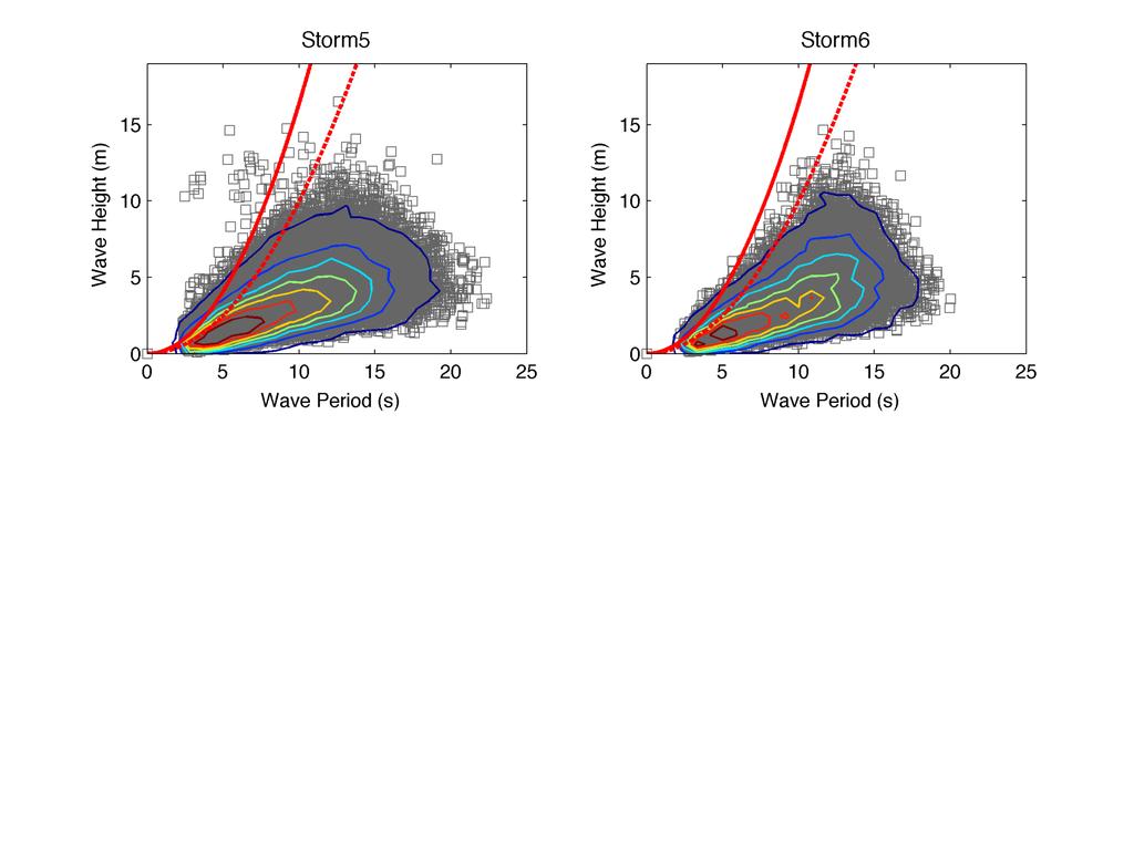
63 50

64 51 Figure 14. Joint distribution of wave height and period for the top ten storms at CDIP station 139 (continued) Figure 15. Joint distribution of wave height and period during calm seas

65 52 As a comparison to data in which waves are not expected to be breaking, Figure 23 shows the joint distribution of waves from several days of data collected during nice weather in the summer (June). While the distribution of periods seems similar to the storms, note that all waves fall below the lower threshold and no breaking is predicted. It is interesting to view how the joint distribution evolves over time. To examine the difference between the different parts of storms, I ve found it useful to plot the joint distribution during each third of a storm. Figures 24 and 25 respectively show these thirds plotted for Storms 1 and 7. For storm 1 we see that the most dangerous waves occur during the first third, longer period waves begin to become more dominant in the middle, and the wave steepness is drastically declined during the final third. During Storm 7 we see that the first third has high waves that are not steep enough for severe breaking, in the middle we see the shape of the distribution change to indicate the arrival Figure 16. Joint distribution during three segments of Storm 1

66 53 of a new wave system, and the final third is dominated by the new wave system which has lower but steeper waves with full breaking expected. Being able to see this evolution and compare it to the significant wave height traces in Figure 19 can help us better understand the nature of each storm. 7.3 The Breaking Severity Factor Distribution Since we want to know about how breaking waves are distributed in a storm and how often they will occur, it is useful to plot the breaking severity factor against its cumulative probability. That is, given n breaking waves in a storm (those above the lower threshold), the probability of the most dangerous wave is 1/n. Such a plot was found to be well fitted by the exponential distribution P(X! B) = e "#B (18) Figure 17. Joint distribution during three segments of Storm 7

67 54 where P(X B) means the probability of the set of breaking waves with a breaking factor greater than or equal to B. The parameter λ indicates how quickly the probability of dangerous waves falls. Given a number of breaking waves, a lower value of λ indicates that more dangerous waves are probable. This distribution is plotted for the top ten storms at station 139 in Figure 26 using a logarithmic scale on the ordinate axis. This plot emphasizes the more dangerous, lower probability waves, and λ is apparent as the slope of each line. The maximum expected breaking factor of a given storm may be calculated by setting the RHS of Equation 18 equal to 1/n and solving for B, such that B max = 1! ln( n) (19) Table 2 lists the parameter λ along with the actual and calculated (or expected) maximum breaking severity factor for the top ten storms. The storms have been sorted by the maximum expected breaking factor, and we see that it can be quite different from the significant height ranking. The expected maximum breaking severity factor was found using Equation 19, where n was the number of predicted breaking waves. While in general the exponential distribution fits the data very well, we see that the larger waves in Storms 3, 5, and 10 diverge significantly from the fit line. Such deviation in some cases is not surprising since the probabilities and numbers of occurrences are very low. Take Storm 3 for example. From Table 2 we see that the maximum measured breaking factor is about 16, coming from a wave 18.9 m high. Finding this wave on the joint distribution in Figure 22 we see that while it is significant, it is clearly an outlier, a chance occurrence that may just as well had a longer period giving it a much lower breaking factor.

68 55

69 56 Figure 18. Breaking severity distribution for the top ten storms at station 139 (continued) 7.4 Other Methods of Obtaining the Joint Distribution Time-series records are not generally available in most cases, and even if they were, they are rather bulky and difficult to handle. Indeed, I spent a good deal of time downloading the ten time-series that I did, having to obtain each chunk separately. It may be useful to derive the joint distribution from more common and compact records, i.e. spectral or parameter records. I will briefly show that spectral records may be used to construct time-series that represents the actual ones quite well. Theoretical parameterbased distributions may also be useful, but may be less certain.

70 57 Table 2. Breaking severity distribution parameters for the top ten storms Hs Rank n Hs Max (m) λ Hmax (m) Recorded Bmax (m) Expected Bmax (m) Time-series Simulation Using Spectra Since the wave spectrum tells us the frequency content of the waves, we can use it to backtrack what the sea surface may have looked like at the time of recording. Every point on the spectrum represents the height of a component wave train at a given frequency, computed directly as H f = 2! F( f )! df (20) where F(f) is the variance density at frequency f and df is the width of the frequency bin. Computing a height for each frequency value results in a bunch of component wave trains. To get a resultant waveform we must assign a phase to each component and then add them all together. The phase is typically taken as random, and must be to avoid unrealistic interference between the components. In equation form, the resultant wave is H (t) = $ H f cos(2! f " # rand ) (21) f If the above procedure is conducted for each spectrum during a storm then a timeseries representing the entire storm may be constructed. The amount of input data needed to construct a joint distribution can thus be greatly reduced: if a storm is 100 spectral records long, each with 64 frequencies, then a total of 6400 numbers are used compared to the roughly 250,000 data points of an equivalent time-series.

71 58 Figure 19. Spectral simulation of the joint distribution during Storm 1. Left: 64 frequency bins. Right: 512 frequency bins An issue that arises in the above procedure is that of uniqueness. Given a limited number of component wave trains, their pattern is likely to repeat in time. In order to get unique information out of each wave, we would like for the waveform not to repeat inside of the time for which it is supposed to be valid (30 to 60 minutes - the time interval of the spectral record). To avoid repetition we need to have more component waves at slightly different frequencies that will have different phases. We can artificially construct these additional waves by splitting each frequency bin into multiple bins, using the same variance density for each of them. While each will have virtually the same height, they will have different phases and slightly different speeds, making the resulting waveform more random in appearance. To illustrate the effect of the frequency splitting procedure, as well as the effectiveness of the simulation technique in general, Figure 27 shows the simulated joint distribution during Storm 1 using two different frequency sets. The left plot was constructed directly with the original spectrum (which has 64 frequency bins). You can see that many of the wave points look duplicated, cheating us out of new, unique information. For the right plot the frequency bins were divided into 8 each (512 total). This plot looks more like one generated by real time-series data. However, I should note that dividing the frequency bins lengthens the computational time. It took under 10 seconds to generate the left plot, and 110 to generate the right-hand plot.