Faculty of Science and Technology MASTER S THESIS. Writer: Rika Afriana

Transcription

1 Faculty of Science and Technology MASTER S THESIS Study program/ Specialization: Offshore Technology/Subsea Technology Spring semester, 2011 Open / Restricted access Writer: Rika Afriana Faculty supervisor: Prof. Ove Tobias Gudmestad External supervisor(s): Prof. Jan Vidar Aarsnes Einar B. Glomnes (Writer s signature) Titel of thesis: Coupled Dynamic Analysis of Cylindrical FPSO, Moorings and Riser Based on Numerical Simulation Credits (ECTS): 30 ECTS Key words: Coupled Dynamic Analysis, Decoupled Analysis, Cylindrical Floater, Moorings, Riser WADAM/HYDRO D, RIFLEX, SIMO, SIMA MARINTEK Pages: 222 pages + enclosure: 159 pages Stavanger, July 28, 2011 Date/year Frontpage for master thesis Faculty of Science and Technology Decision made by the Dean October 30 th 2009

2 1 Abstract M.S.c. Thesis Coupled Dynamic Analysis of Cylindrical FPSO, Moorings and Riser Based on Numerical Simulation The hostile environments are presently one of the challenges that should to be deal with in offshore floating system design where the hydrodynamic interaction effects and dynamic responses dominate the major consideration in its design. Nowadays, the cylindrical FPSO is being extensively used as an offshore facility in the oil and gas industry. This system has been deployed widely around the world as a unique design facility which is regarded as a promising concept. As a floating offshore system, a cylindrical FPSO will be deployed together with slender members (moorings and risers) responding to wind, wave and current loading in complex ways. In order to quantify the coupling effects between each component in an offshore floating system and the associated structural response in offshore structure design, two kind of analyses, the decoupled analysis and the nonlinear coupled dynamic analysis have been presented in this thesis. It introduces a consistent analytical approach that ensures higher dynamic interaction between the floater, moorings and risers. The nonlinear coupled dynamic analysis requires a complete model of the floating offshore system including the cylindrical S400 floater, 12 mooring lines and the feasible riser configurations for the 6 and 8 production risers. Furthermore, the results from the nonlinear coupled dynamic analysis will also be compared to the separated analyses for each component as a discussion of the analysis results. The frequency domain and time domain analysis will be implemented to solve the equation of motions at the simulations. The simulation will be conducted in two simulation schemes, static and dynamic conditions. The 3 hours + build up time will be used in the dynamic condition because the time domain requires a proper simulation length to have a steady result. Several software computer programs will be used in the analyses. In the separated analysis for each component in offshore floating system, the cylindrical floater hydrodynamic analysis as a decoupled analysis is performed by using the integrated software program Hydro D which is related to several support software programs (Prefem, Wadam and Postresp). For mooring system analysis as a decoupled analysis will be analyzed by using SIMO in time domain analysis. In SIMO, two models (the body model and the station keeping model) will be required and the quasi static design will be applied as the design method in mooring system analysis. The analysis for riser system also is done as the decoupled analysis in this study. The main purpose of this analysis is to find a feasible single arbitrary configuration for ii

3 each of the 6 and 8 production risers. The riser system analysis will also be performed in time domain analysis in RIFLEX for two simulation conditions, static and dynamic conditions. After the separated analyses for each component, a single complete computer model that includes a cylindrical floater, moorings and risers with use of SIMA will be as the nonlinearcoupled dynamic analysis. The analysis is performed in time domain for two conditions, static and dynamic conditions. The SIMA Marintek computer will be used in this study because it has the capability to integrate the cylindrical S400 floater, moorings and risers as one complete model. As an integrated dynamic system, the environmental forces on the floater induce the motions which will be introduced in a detail FEM (Finite Element Model) of the moorings, risers and cylindrical S400 floater. In the end, not only the accurate prediction of the responses of the overall system but also the individual responses of the floater, mooring and risers are obtained. The summary of results between the decoupled analysis and the nonlinear coupled dynamic analysis will also be presented briefly in this study. iii

4 1 Acknowledgement M.S.c. Thesis Coupled Dynamic Analysis of Cylindrical FPSO, Moorings and Riser Based on Numerical Simulation This thesis is the final work of my graduate study at the Department of Offshore Technology, Faculty of Natural Science and Technology, University of Stavanger, Norway. The thesis has been carried out from February until June 2011 at the Research and Development Department in Sevan Marine AS, Arendal. I would like to acknowledge and extend my heartfelt gratitude to the following persons who have made the completion of this thesis possible: My supervisor, Professor Ove T. Gudmestad for his interest to this thesis and for his great motivation to me. Without his encouragement, guidance and endless supports, this thesis would not have been accomplished. Life blessed me with a lot of opportunity after I met him. My supervisor in Sevan Marine AS, Professor Jan V. Aarsnes for his advices during this study. My supervisor, Einar B. Glomnes who always helpful and willing to take some time togive me his guidances. His advices and knowledge are very valuable for this thesis. Kåre Syvertsen, for giving me the opportunity and providing me with so many valuable facilities during the thesis work at the Research and Development Department in Sevan Marine AS, Arendal. Kåre G. Breivik, for giving me the opportunity to write my thesis at the Research and Development Department in Sevan Marine AS, Arendal. Knot Mo and Elizabeth Passano from Marintek, for providing guidance regarding SIMA Marintek computer software. The people from the Research and Development Department Sevan Marine AS for giving me such a wonderful experience during this study. Tor Stokke, Irina Kjærstad, Torhild Konnestad, Alf Reidar Sandstad, Veslemøy U. Sandstad, Per Høyum. All of my friends in University of Stavanger, Norway for they supportive and fun filled environment during our study period in University of Stavanger. For Indonesian heroes this year: Iswan Herlianto, Adri Maijoni, Eko Yudhi Purwanto, Sari Savitri, Winia Farida and Dian Ekawati. We have to be very proud for our achievements. The special thanks for Adedayo Adebayo, Tonje Charlotte Stald, Morten Langhelle, Henry Ezeanaka, Bamidele Oyewole, Mina Jalali, Markus Humel, Jarle Gundersen, Ragnhild O Steigen, Sahr M. Hussain, Farhia B. Nur, Rakhshinda Ahmad and Fery Simbolon, Tomy Nurwanto, Hermanto Ang, Yahya Januarilham, iv

5 Surya Dharma, Sakti Tanripada, Sanggi Raksagati. Our university can t be homie without you guys. Hans Marthyn Franky Panjaitan, Iqbal Ruswandi, Dilly Soemantri, Ahmad Makintha Brany, Airindy Felisita, Maurina Adriana, Agung Ertanto, Miftachul Choiri, Ronny Costamte, Novithasari Dewi Anggraeni, Trimaharika Widarena and Ratna Nita Perwitasari. Many thanks for the guidance and valuable advices. Apak and Amak, for teaching me the love of science and the belief that almost anything can be accomplished through hard work and determination. I especially dedicated this thesis for them. My brother and sister for their warm supports. My loving, supportive, encouraging, and patient soulmate Indra Permana whose faithful and always give me his endless support from the beginning till the end of time. This thesis would not have been possible without his contributions. Thank you for always believe in me to chase my dream and pursuit our happiness. Happy wedding! I offer my regards to all of those who supported me in any respect during the completion of this study. Finally, my greatest regards to Allah SWT for bestowing upon me the courage to face the complexities of life and complete this thesis. Rika Afriana v

6 Table of Contents M.S.c. Thesis Coupled Dynamic Analysis of Cylindrical FPSO, Moorings and Riser Based on Numerical Simulation Abstract... ii Acknowledgement... iv Tables of Contents... vi List of Figures... ix List of Tables... xv Chapter 1 Chapter 2 Chapter 3 Introduction 1.1 Background State of Art Problem Statement Purpose and Scope Location of Study Theoretical Background 2.1 Equation of Motion for Floating Structure Response of Single Body Structures Second-Order Nonlinear Problems The Mean Wave (Drift) Forces The Slowly Varying (Low frequency) Wave Forces Frequency Domain and Time Domain Analysis Frequency Domain Analysis Time Domain Analysis Fundamental Continuum Mechanics Theory and Implementation of the Finite Element Method Fundamental Continuum Mechanics Theory Implementation of the Finite Element Method Coupling Effects Environmental Conditions 3.1 Water Level Winds The Wind Force Simulated In Time Domain vi

7 3.3 Waves Regular waves Irregular Waves Currents The Current Force Simulated In Time Domain Heading Dependency of Environmental Conditions Chapter 4 Chapter 5 Chapter 6 Chapter 7 Chapter 8 Methodology of the Analysis 4.1 System Components Method Analysis of Nonlinear-coupled dynamic Numerical Simulation Steps Hydrodynamic Analysis of Cylindrical FPSO S General Description Model Concept and Analysis Steps Hydrodynamic Response and Stability Analysis Stability Analysis Transfer Functions Mean Wave (Drift) Force Nonlinear Damping Effect Moorings Analysis 6.1 Mooring Systems Mooring System Design Basic Theory for Design Design Criteria Modeling Concept and Analysis Steps Moorings Analysis Static Condition Dynamic Condition Riser Analysis 7.1 Production Riser Systems Flexible Riser Design in Shallow Water and Harsh Environments Riser Configuration Selections Design Parameters Design Criterion Methodology Design and Analysis Steps The Western Isles Field Layout and Model Properties for the Riser System Modeling Concept by RIFLEX Riser Analysis Layout and Schematic Riser Configuration Static Condition Dynamic Condition Coupled Dynamic Analysis 8.1 Modeling Concept by SIMA Marintek vii

8 8.2 The System Response in the Nonlinear-Coupled Dynamic Analysis Floater Motions The Horizontal Offset Values The Nonlinear-Coupled Dynamic Analysis for Slender Members Chapter 9 Conclusions and Further Studies 9.1 Conclusions Further Studies References Appendix A Appendix B Appendix C Appendix D Appendix E Appendix F Response Amplitude Operator (RAO) Wave Drift Force System Description SIMO Riflex Decoupled Input SIMA (RIFLEX+SIMO) Coupled Input Hydro D Model viii

9 List of Figures M.S.c. Thesis Coupled Dynamic Analysis of Cylindrical FPSO, Moorings and Riser Based on Numerical Simulation Figure 1.1 : Floating offshore structure Figure 1.2 : Field overview Figure 2.1 : Definition of rigid-body motion modes Figure 2.2 : Superposition of hydro mechanical and wave loads Figure 2.3 : The relation between the waves and the motions Figure 2.4 : Motion of a material particle Figure 2.5 : Nodal point with translational and rotational degrees of freedom Figure 2.6 : Bar element in initial and deformed configuration Figure 2.7 : Nodal degrees of freedom for beam element Figure 2.8 : Prismatic beam Figure 3.1 : Definition of location and measurement points for metocean data Figure 3.2 : ISO wind spectrum for a mean wind speed of 20 m/s. In the SIMO Figure 3.3 : Harmonic wave definitions Figure 3.4 : Atmospheric pressure at the free surface Figure 3.5 : Sinusoidal wave profile Figure 3.6 : Surface wave definitions based on WADAM Figure 3.7 : The data for regular waves calculation in WADAM analysis Figure 3.8 : Directional relative magnitudes of significant wave height Figure 3.9 : Hs/Tp Omni directional Hs-Tp contour for the 100-years return period sea state Figure 3.10 : Jonswap spectrum Figure 3.11 : Torsethaugen spectrum Figure 3.12 : Ten years directional current profile. Directions are towards which current is flowing Figure 3.13 : The distribution of heading probability of the environmental parameters ix

10 Figure 3.14 : 100-years return period design significant wave height and wind speed Figure 4.1 : Illustration of traditional separated analysis; de-coupled analysis Figure 4.2 : Schematic for nonlinear-coupled dynamic analysis Figure 4.3 : Coupled floater motion and slender structure analysis Figure 4.4 : An integrated scheme analysis Figure 4.5 : Load cases combinations scheme analysis Figure 5.1 : S400 FPSO - 3D model Figure 5.2 : S400 FPSO - 2D model Figure 5.3 : Overview of model types Figure 5.4 : S400 FPSO - 2D model Figure 5.5 : The relation between Prefem, Wadam and Postresp as an integrated program for analysis of a cylindrical floater S Figure 5.6 : A simple procedure for the hydrodynamic analysis for a cylindrical floater S Figure 5.7 : Hydro model combinations Figure 5.8 : Finite element models for a cylindrical floater S Figure 5.9 : The data for the Wadam mass models for the cylindrical floater S Figure 5.10 : The hydrodynamic properties for the Wadam mass model Figure 5.11 : The appearance of HydroD Figure 5.12 : A cylindrical floater model of S400 model in HydroD Figure 5.13 : Inclined a cylindrical floater S Figure 5.14 : The movement of GM from the ballasted to fully loaded condition Figure 5.15 : The amplitude of the response variable for surge in regular wave condition Figure 5.16 : The amplitude of the response variable for sway in regular wave condition Figure 5.17 : The amplitude of the response variable for heave in regular wave condition Figure 5.18 : The amplitude of the response variable for roll in regular wave condition Figure 5.19 : The amplitude of the response variable for pitch in regular wave condition Figure 5.20 : The amplitude of the response variable for yaw in regular wave condition Figure 5.21 : The amplitude of the response variable for surge in irregular wave condition Figure 5.22 : The amplitude of the response variable for sway in irregular wave condition Figure 5.23 : The amplitude of the response variable for roll in irregular wave condition Figure 5.24 : The amplitude of the response variable for pitch in irregular wave condition Figure 5.25 : The amplitude of the response variable for yaw in irregular wave condition Figure 5.26 : The drift force-far field versus the pressure integration in surge for regular waves Figure 5.27 : The drift force, far field versus the pressure integration in sway for regular waves x

11 Figure 5.28 : The drift moment, far field versus the pressure integration in yaw for regular waves Figure 5.29 : The drift force, pressure integration in heave for regular waves Figure 5.30 : The drift moment, pressure integration in roll for regular waves Figure 5.31 : The drift moment, pressure integration in pitch for regular waves Figure 5.32 : The drift force, far field versus pressure integration in surge for irregular waves Figure 5.33 : The drift force, far field versus pressure integration in sway for irregular waves Figure 5.34 : The drift moment, far field versus pressure integration in yaw for irregular waves Figure 5.35 : The drift force, pressure integration in heave for irregular waves Figure 5.36 : The drift moment, pressure integration in roll for irregular waves Figure 5.37 : The drift moment, pressure integration in pitch for irregular waves Figure 5.38 : The non linear damping effect in surge for regular wave Figure 5.39 : The non linear damping effect in sway for regular wave Figure 5.40 : The non linear damping effect in heave for regular wave Figure 5.41 : The non linear damping effect in roll for regular wave Figure 5.42 : The non linear damping effect in pitch for regular wave Figure 5.43 : The non linear damping effect in yaw for regular wave Figure 6.1 : Environmental forces acting on a moored vessel in head conditions and the transverse motion of catenary mooring lines Figure 6.2 : Mooring lines layout overview Figure 6.3 : Mooring line composition Figure 6.4 : The movable winch on a cylindrical S400 floater Figure 6.5 : The combined fairlead/chain stopper on a cylindrical S400 floater Figure 6.6 : The cable line with symbols Figure 6.7 : The forces acting on an element of mooring line Figure 6.8 : A simple procedure for mooring analysis Figure 6.9 : The structural mass data for a cylindrical S400 floater Figure 6.10 : Layout of the SIMO program system and file communication between modules Figure 6.11 : The calculation parameters for static and dynamic condition Figure 6.12 : The global motion response, the low frequency motions for surge Figure 6.13 : The global motion response, the low frequency motions for sway Figure 6.14 : The global motion response, the low frequency motions for heave Figure 6.15 : The global motion response, the low frequency motions for roll xi

12 Figure 6.16 : The global motion response, the low frequency motions for pitch Figure 6.17 : The global motion response, the low frequency motions for yaw Figure 6.18 : The total global motion response, the total frequency motions for surge Figure 6.19 : The total global motion response, the total frequency motions for sway Figure 6.20 : The total global motion response, the total frequency motions for heave Figure 6.21 : The total global motion response, the total frequency motions for roll Figure 6.22 : The total global motion response, the total frequency motions for pitch Figure 6.23 : The total global motion response, the total frequency motions for roll Figure 6.24 : The mooring line dynamic tensions in time series for S400_Line Figure 6.25 : The mooring line dynamic tensions in time series for S400_Line Figure 6.26 : The mooring line dynamic tensions in time series for S400_Line Figure 6.27 : The mooring line dynamic tensions in time series for S400_Line Figure 6.28 : The mooring line dynamic tensions in time series for S400_Line Figure 6.29 : The mooring line dynamic tensions in time series for S400_Line Figure 6.30 : The mooring line dynamic tensions in time series for S400_Line Figure 6.31 : The mooring line dynamic tensions in time series for S400_Line Figure 6.32 : The mooring line dynamic tensions in time series for S400_Line Figure 6.33 : The mooring line dynamic tensions in time series for S400_Line Figure 6.34 : The mooring line dynamic tensions in time series for S400_Line Figure 6.35 : The mooring line dynamic tensions in time series for S400_Line Figure 6.36 : The second order wave forces XR Forces (in Surge) Figure 6.37 : The second order wave forces YR Forces (in Sway) Figure 6.38 : The second order wave moment Moment ZR axis (in Yaw) Figure 6.39 : The drift damping forces XR Forces (in Surge) Figure 6.40 : The drift damping forces YR Forces (in Sway) Figure 6.41 : The drift damping forces moment ZR axis (in Yaw) Figure 7.1 : Examples of riser systems Figure 7.2 : Flexible riser Figure 7.3 : Standard flexible riser configurations Figure 7.4 : The influence of vessel offset in riser design Figure 7.5 : Methodology design for a riser system Figure 7.6 : The riser system for South Drill Centre Figure 7.7 : Layout of the RIFLEX program system and file communication between modules Figure 7.8 : System definition for the description of the layout configuration design xii

13 of the Arbitrary Riser system configuration (AR) Figure 7.9 : The riser configuration of the 6 production riser for the Western Isle Field Figure 7.10 : The riser configuration of the 8 production riser for the Western Isle Field Figure 7.11 : The static effective tension for the 6 production riser for the Western Isle Field Figure 7.12 : The static effective tension for the 8 production riser for the Western Isle Field Figure 7.13 : The static bending moment for the 6 production riser for the Western Isle Field Figure 7.14 : The static bending moment for the 8 production riser for the Western Isle Field Figure 7.15 : The static curvatures for the 6 production riser for the Western Isle Field Figure 7.16 : The static curvatures for the 8 production riser for the Western Isle Field Figure 7.17 : The displacement envelope curvature for the 6 production riser Figure 7.18 : The displacement envelope curvature for the 8 production riser Figure 7.19 : The dynamic effective tension for the 6 production riser for the Western Isle Field Figure 7.20 : The dynamic effective tension for the 8 production riser for the Western Isle Field Figure 7.21 : The dynamic bending moment for the 6 production riser for the Western Isle Field Figure 7.22 : The dynamic bending moment for the 8 production riser for the Western Isle Field Figure 7.23 : The dynamic curvatures for the 6 production riser for the Western Isle Field Figure 7.24 : The dynamic curvatures for the 8 production riser for the Western Isle Field Figure 8.1 : Library data system of the SIMA Marintek Figure 8.2 : The total global motion response, the total frequency motions for surge Figure 8.3 : The total global motion response, the total frequency motions for sway Figure 8.4 : The total global motion response, the total frequency motions for heave Figure 8.5 : The total global motion response, the total frequency motions for roll Figure 8.6 : The total global motion response, the total frequency motions for pitch Figure 8.7 : The total global motion response, the total frequency motions for yaw Figure 8.8 : The total global motion response, the total frequency motions for surge from the station keeping system modeling in SIMO (Chapter 6) Figure 8.9 : The static effective tension for the 6 production riser for the Western Isle Field in the nonlinear-coupled dynamic analysis Figure 8.10 : The static effective tension for the 8 production riser for the Western Isle Field in the nonlinear-coupled dynamic analysis Figure 8.11 : The static bending moment for the 6 production riser for the Western Isle xiii

14 Field in the nonlinear-coupled dynamic analysis Figure 8.12 : The static bending moment for the 8 production riser for the Western Isle Field in the nonlinear-coupled dynamic analysis Figure 8.13 : The static curvatures for the 6 production riser for the Western Isle Field in the nonlinear-coupled dynamic analysis Figure 8.14 : The static curvatures for the 8 production riser for the Western Isle Field in the nonlinear-coupled dynamic analysis Figure 8.15 : The displacement envelope curvature for the 6 production riser Figure 8.16 : The displacement envelope curvature for the 8 production riser Figure 8.17 : The dynamic effective tension for the 6 production riser for the Western Isle Field in the nonlinear-coupled dynamic analysis Figure 8.18 : The dynamic effective tension for the 8 production riser for the Western Isle Field in the nonlinear-coupled dynamic analysis Figure 8.19 : The dynamic bending moment for the 6 production riser for the Western Isle Field in the nonlinear-coupled dynamic analysis Figure 8.20 : The dynamic bending moment for the 8 production riser for the Western Isle Field in the nonlinear-coupled dynamic analysis Figure 8.21 : The dynamic curvatures for the 6 production riser for the Western Isle Field in the nonlinear-coupled dynamic analysis Figure 8.22 : The dynamic curvatures for the 8 production riser for the Western Isle Field in the nonlinear-coupled dynamic analysis xiv

15 List of Tables M.S.c. Thesis Coupled Dynamic Analysis of Cylindrical FPSO, Moorings and Riser Based on Numerical Simulation Table 3.1 : NORSOK Guidance Return Period Combinations in the Design Table 3.2 : Still Water Levels, Surges and Still Water Depths Based on a Nominal LAT Depth Table 3.3 : Extreme Water Levels and Depths Based on a Nominal LAT Depth Table 3.4 : Extreme Wind Speeds at 10 m asl- by Direction (From) Table 3.5 : Extreme Wind Speeds at 10 m asl- Omnidirectional Table 3.6 : Directional hs Relative magnitudes Table 3.7 : Extreme Wave Criteria for eight directional Table 3.8 : Extreme Wave Height and Asscociated Periods- Omnidirectional Table 3.9 : Tide, Surge and Total Directional Depth Averaged Currents (cm/s) Table 3.10 : Extreme Total Current Profile (m/s) - by direction (direction are towards) Table 3.11 : The used design environmental conditions for return period condition Table 5.1 : S400 FPSO Main Particulars Table 5.2 : The Damping and Restoring Matrices for the Ballasted Loading Condition Table 5.3 : The Damping and Restoring matrices for the fully loaded condition Table 5.4 : The mass properties for ballasted condition Table 5.5 : The hydrostatic data for ballasted condition Table 5.6 : The mass properties for fully loaded condition Table 5.7 : The hydrostatic data for fully loaded condition Table 6.1 : Mooring Line Composition for Sevan 400 FPSO Table 6.2 : The Detailed Orientation and The Pretension of The Lines Table 6.3 : ULS Line Tension Limits and Design Safety Factors Table 6.4 : The Linear Damping Coefficients for Mooring Analysis Table 6.5 : The Quadratic Damping Coefficients for Mooring Analysis xv

16 Table 6.6 : The Linear Hydrostatic Stiffness Matrix for Mooring Analysis (kg.m/s2) Table 6.7 : The Quadratic Current Coefficients for 6 DOF Motions From 0 to Table 6.8 : The Wind Coefficients for 6 DOF Motions From 0 to Table 6.9 : The Wave Drift Damping Coefficients Table 6.10 : The Wave Drift Damping Coefficients Table 6.11 : The Final Static Body Position of A Cylindrical S400 Floater Table 6.12 : The Static Forces and Moments on S400 Floater Table 6.13 : The Mooring Line Static Tensions Table 6.14 : The Summary of The Global Motion Response of A Cylindrical S400 Floater Table 6.15 : The Summary of Mooring Line Dynamic Tensions of a cylindrical S400 floater Table 6.16 : The Summary of Line Tension Limit and Design Safety Factor Table 6.17 : The Summary of Second Order Wave Forces Table 6.18 : The Summary of wave drift damping forces Table 7.1 : Design MBR requirements Table 7.2 : Physical Properties for Risers Table 7.3 : Physical Properties for Risers Table 8.1 : The EVA Analysis Results for 100 Years Waves Table 8.2 : Extreme Wave Height and Associated Periods- Omnidirectional Table 8.3 : The Summary of The Global Motion Response of A Cylindrical S400 Floater in the Nonlinear-Coupled Dynamic Analysis Table 8.4 : The Summary of The Global Motion Response of the Cylindrical S400 Floater in the Nonlinear-Coupled Dynamic Analysis and the Station Keeping System Modeling results as found from SIMO (Chapter 6) Table 8.5 : The summary of mooring line dynamic tensions of the cylindrical S400 floater in the nonlinear-coupled dynamic analysis Table 9.1 Table 9.2 : The Summary of The Global Motion Response of A Cylindrical S400 Floater in the Nonlinear-Coupled Dynamic Analysis and the Station Keeping System Modeling results as found from SIMO (Chapter 6) : The Summary of Mooring Line Dynamic Tensions in The Nonlinear-Coupled Dynamic Analysis and Mooring Line Dynamic Tensions Results as Found from SIMO (Chapter 6) xvi

17 Chapter 1 1 Introduction M.S.c. Thesis Coupled Dynamic Analysis of Cylindrical FPSO, Moorings and Riser Based on Numerical Simulation 1.1 Background Nowadays, the cylindrical FPSO is being extensively used as an offshore facility in the oil and gas industry. This system has been deployed widely around the world as a unique design facility which is regarded as a promising concept for an economic oil production since it has capability for storage and wider deck that is giving better layout flexibility. Moreover, it has also the ability to move and relocate after the operation is completed and is suitable for all offshore environments meeting the challenges of the oil and gas industry. As a floating offshore system, a cylindrical FPSO will be deployed together with slender members (moorings and risers) responding to wind, wave and current loading in complex ways. In the traditional way, the hydrodynamic interaction among the floater, moorings and risers cannot be evaluated since the floater, moorings and risers are treated separately. Moreover, this traditional method, also known as the decoupled analysis, the hydrodynamic behavior of the system is only based on hydrodynamic behavior of the hull and ignores all or part of the interaction effects (mass, damping, stiffness, current loads) between the floater, moorings and risers. In order to capture the interaction between the floater, moorings and risers, one extensive method has been introduced and developed in the last decade. This method, also known as the nonlinear coupled dynamic analysis, ensures higher dynamic interaction among the components responding to environmental loading due to wind, waves and currents since the main coupling effects will be included automatically in the analysis. Hence, the accurate prediction of the response for the overall system as well as the individual response of floater, moorings and risers can be obtained. Lately, the nonlinear coupled dynamic analysis of the floating systems is becoming more and more important in order to evaluate the dynamic interaction among the floater, moorings and risers. Extensive work during last decade has been performed by many researches. Most of their implementations that are related to the study will be presented below: Omberg and Larsen (1998) concluded that the uncoupled analysis may produce severely inaccurate results. Besides that, Kim and Kim (2002) have investigated the global motion of a 1-1

18 turret moored FPSO with 12 chain polyester chain mooring lines and 13 steel catenary risers in a fully coupled hull/mooring/riser dynamic analysis and concluded that the coupled behavior of vessel, moorings and riser will greatly enhance the understanding of the relevant physics and the overall performance assessment of the system. Furthermore, Chaudry and Yo Ho (2000) concluded that the full coupling of dynamic equilibrium in actual motions will be important for moorings and risers motion since the coupling effects give significant influence to the motion of moorings and risers. Based on the reasons above, the nonlinear coupled dynamic analysis has been addressed as the proper strategy to improve the understanding of the overall hydrodynamic behavior. This analysis will ensure higher dynamic interaction between the vessel and the slender system because of two reasons: The overall behavior of the floater will be influenced not only from the hydrodynamic behavior of the hull but also from the dynamic behavior of the slender members (moorings and risers) The coupling effects such as restoring, damping and added mass will be taken into account automatically in the process of analysis. Hence, the nonlinear coupled dynamic analysis represents a truly integrated system which ensures accurate prediction of all motions and responses without imposing conservatism. In the study, the Western Isles Development Project (WIDP) that is located in the UKCS, Block 210/24 to the North East of Shetland will be taken as reference case. Moreover, the WIDP has shallow water conditions and also has harsh environment. These two major characteristics will influence the design of the overall system of the floating offshore system. Furthermore, the study has been performed at the Research and Development Department in Sevan Marine AS, Arendal from February until June All of information in this project is confidential. 1.2 State of Art Offshore structures are located in the ocean environments without continuous access to dry land and this causes offshore structures to have hydrodynamic interaction effects and dynamic response as major considerations for their design. They may be required to stay in position in all weather conditions. The configuration of an offshore structure may be classified by whether the structure is a fixed structure or floating structure. Chakrabarti (2010) has mentioned that the requirements for a floating structure are that it should be moored in place and that the facility under the action from the environment remains within a specified distance from a desired location achieved by the station keeping. A floating offshore system consists of three principal structural components (Figure 1.1): 1. Floating hull: facilitating the space for the operations of the production work and storage for supplies 2. The station keeping: providing a connection between the structure and the seafloor for the purposes of securing the structure against the environmental loads, and 3. Riser system: achieving drilling operations or product transport 1-2

19 Figure 1.1 : Floating offshore structure. Reference: Chakrabarti, 2010 The station keeping may also be achieved by a dynamic positioning system solely using thrusters or in combination with mooring lines. The mooring lines and risers provide restoring forces to the floater. Coupled versus Decoupled Analysis Traditionally, the offshore industry has used de coupled analysis as the methodology for design of floating offshore platforms with moorings and risers. Nowadays, a lot of researches have suggested that the integration between the floating hull, mooring and the risers as a dynamic system is important in order to capture the interaction between them and obtain realistic motion values for each individual system. Omberg et al. (1997 and 1998) concluded that the design of a Floater Production System (FPS) should consider the fact that the moored system and the risers comprise a truly integrated system; that is the overall behavior of the floating system is dictated not only by the hydrodynamic behavior of the hull but also by its interaction with the hydrodynamic/structural behavior of the lines. Another suggestion has been presented by Chakrabarti (2008) regarding a specific recommendation for the systematic proces of the coupled analysis. The de coupled analysis Based on DNV definition, DNV RP F205 (2010), a de coupled analysis is performed of the floater motion in time domain, but the effects of the mooring and riser system are included quasi statically using non linear springs, i.e. having quasi static restoring force characteristic. All other coupling effects such as contribution damping and current loading on the slender structures, need to be given as input to the analysis based on a separate assessment. 1-3

20 Chakrabarti (2008) explained that the de coupled analysis represents the traditional methodology, in which the numerical analysis tool is based on the hydrodynamic behavior of the floater, uninfluenced by the nonlinear dynamic behavior of moorings or riser. Generally, little or no integration between the moored system and the riser takes place. It is still the common design practice for floating production systems. The coupled analysis On the other hand, based on DNV RP F205 (2010), the complete system of equations accounting for the rigid body model of the floater as well as the slender body model for the risers and mooring lines are solved simultaneously using a non linear time domain approach for the dynamic analysis. Dynamic equilibrium is obtained by the time domain approach at each time step ensuring consistent treatment of the floater/slender structure coupling effect. The coupling effects are automatically included in the analysis scheme. Specifically, the response of each component in such a system is influenced by the mechanical and hydrodynamic coupling effect and the proximity to the other components. Hence, all relevant coupling effects will be analyzed. The floater, moorings and risers system comprise an integrated dynamic system responding to environmental loadings due to wind, waves and currents. In an integrated dynamic system, the environmental forces on the floater induce the motions which will be introduced in a detailed finite element model of the moorings and risers. Furthermore, the coupled analysis will verify the integrations of radiation/diffraction theory with a beam finite element technique in time domain scenario analysis. With reference to Connaire et al (2003), a coupled analysis capability has been developed and extensively verified, which integrates radiation/diffraction theory with a beam finite element time dependent structural analysis technique for slender offshore structures. 1.3 Problem Statement As oil and gas exploitations move to deepwater and more harsh environment, the hydrodynamic integration between the floating hull, mooring and the risers as a dynamic system will be complex and become important. Hence, more advance methodologies are needed to provide a much deeper understanding of the system behavior. Moreover, the capacity to analyze and model test for this situation are challenged. Efficient tools and procedures on how to determine dimensioning response will be needed. This study will emphasize on how to perform the nonlinear coupled analysis of the floater, moorings and risers with efficient tools and procedures in order to capture the interaction between the floater, moorings and risers. This study will present a consistent analytical approach to ensure higher dynamic interaction between floater, moorings and risers. As a consistent analytical approach, the study will implement numerical simulation steps by using several analysis programs such as Wadam/HYDRO D, SIMO and RIFLEX for an integrated program analysis. A single and complete model will include a cylindrical S400 floater, 12 mooring lines and one of feasible riser configurations. The detailed model for each component, characterization of the environments in covering relevant load models and the simulation schemes will be presented in this study. 1-4

21 The analysis will be performed in the frequency domain and time domain in order to solve the problems during the analysis. 1.4 Purpose and Scope The objective of the study is to document a consistent analytical approach for the nonlinearcoupled analysis of the floater, moorings and risers that ensure higher dynamic interaction between floater, moorings and risers. Generally, the study will cover the following activities below: 1. The study of literature for a floating offshore system and each component, cylindrical FPSO, moorings and risers and the therotical background that provides deeper understanding on a consistent analytical approach for the numerical simulations. 2. The study of literature for the basic theory of Wadam/HYDRO D, SIMO and RIFLEX and other complementary programs such as PREFEM, POSTRESP and ORCAFLEX. 3. The nonlinear coupled analysis perfomance in SIMA. Chapter 2 presents the theoretical background that will be helpful to give the perspective for the analysis. The basic knowledge and key definitions that relate to the analysis will be presented here. Chapter 3 presents the specification of data from the environment based on metaocean design criteria. The environmental conditions such as water depth, wind, waves and currents will be presented here. Chapter 4 presents the methodology of the analysis. This chapter will explain the analysis procedures for system components, analysis method for nonlinear coupled dynamic analysis and the numerical simulation steps in the nonlinear coupled dynamic analysis. The analysis will be performed by using several programs such as Wadam/Hydro D, RIFLEX and SIMO. These programs will be used under an integrated scheme analysis to obtain a consistent analytical approach for the nonlinear coupled dynamic analysis. Chapter 5 presents the hydrodynamic analysis of the cylindrical S400 FPSO. The general description of the cylindrical S400 FPSO will be presented here. This chapter will present the analysis of the floater s load model based on diffraction theory to obtain the transfer function, mean wave drift forces and non linear damping. Furthermore, the analysis will be performed by using a diffraction program, Wadam/HYDRO D. The resulting analysis will not only present on the hydrodynamic but also the stability of the cylindrical floater. The hydrodynamic analysis of the hull is performed in the frequency domain analysis as a simple iterative technique to solve a linear equation of motions to obtain a set frequency dependent RAO. Chapter 6 presents the general description and configuration of the moorings that will be used in the analysis. This chapter will also present the combined model between cylindrical floater and moorings in time domain analysis by using SIMO. In this analysis, the effect of wind and currents will be considered. SIMO as a computer software program for moored vessels will be used in order to include the mooring stiffness in the equation of the motions. Therefore, motions are found by time integration enforcing force equilibrium at all time steps. The corresponding mooring line tensions are established using a quasi static approach. 1-5

22 The result of the analysis will give us the result of a set of time series of the offset vessel value under LF motions and also the total motions (LF+WF motions). Chapter 7 presents a feasible arbitrary riser configuration. The investigations of the riser configurations will use RIFLEX. Furthermore, the investigation will be performed under decoupled analysis to obtain a single arbitrary configuration. The analysis will also be performed in time domain under two simulation schemes, static and dynamic conditions. A discussion of the analysis results such as top angle (hang off position angle), effective tension, bending radius and seabed clearance will be presented here. Chapter 8 presents a single complete model that includes the cylindrical floater, moorings and riser by using SIMA Marintek computer software. In principle, the SIMA will combine two nonlinear numerical simulations together those obtained by SIMO and RIFLEX. In other words, the cylindrical floater and moorings model from SIMO will be combined together with an arbitrary riser configuration from RIFLEX in time domain analysis. The results of the analysis will be a set of accurate predictions for floater motions as well as the moorings and riser system with regard to the coupling effects. Furthermore, the resulting analysis for the riser will be presented and compared with the previous analysis based on the decoupled analysis from Chapter 6 and Chapter 7. Chapter 9 provides the conclusions and the recommended further studies from this study. 1.5 Location of Study An overview of the location can be seen in Figure 1.2, Dana Petroleum E&P Limited (2011) has mentioned that the offshore field Western Isles is located in the UKCS Block 210/24 to the North East of Shetland. The nearest fixed facility is the Tern platform located 12 km East of Western Isles. The Western Isles Field is located approximately 61º N, 0º E. Moreover, the offshore Western Isles Field is located in relatively on shallow water condition and also harsh environment. The water depth is approximately 170 m. The design life is specified to be 20 years. 1-6

23 Figure 1.2 : Field overview. Reference: Dana Petroleum E&P Limited (2011) 1-7

24 Chapter 2 1 Theoretical Background M.S.c. Thesis Coupled Dynamic Analysis of Cylindrical FPSO, Moorings and Riser Based on Numerical Simulation This chapter will review the basic knowledge to give a perspective for the analysis. Moreover the key definitions that are related to the analysis will also be explained here. The explanation about the equation of motion will be the starting point then we will continue to the structure response, non linear problems, frequency domain analysis and time domain, fundamental continuum mechanics and implementation of finite element method, and finaly coupling effects. 2.1 Equation of Motion for Floating Structure Before the further explanation about the equation of motion for the floater, the relation between the motion of the floater and the influence on its responses will be presented below: A floater is almost always taken as a 6 DOF (degrees of freedom) rigid body motions model for its response calculations. The basic theory about this can be clearly found in Faltinsen (1990). Further, the oscillatory rigid body translation motions can be referred to as surge, sway and heave while the oscillatory angular motions are referred to as roll, pitch and yaw based on Figure 2.1. below: Figure 2.1. : Definition of rigid body motion modes. Reference: Journée and Massie (2001) For the analyses of the floater motions it is needed to consider the different hydrodynamic effects on the floater. Generally, a structure responds to environmental forces due to wind, waves and currents with motions on three different time scales; Wave Frequency (WF), Low 2-1

25 Frequency (LF) and High Frequency (HF). The inviscous fluid effects mostly govern the wave frequency and high frequency motions while the low frequency motion will be determined by the viscous fluid effects. The wave frequency motions (WF) are generated by the wave forces on the floater while the low frequency motions (LF) are driven by the mean wave (drift) and slowly varying forces from waves or currents. On the other hand, the higher order wave forces result from the high frequency motion (HF) that may induce springing or ringing response (DNV RP F205 (2010)). Normally, a moored floater is dynamically excited by ordinary wave frequency load but also exposed to the mean wave (drift) and slowly varying forces from waves or currents. Løken et al. (1999) mentioned that the dynamic equations of equilibrium forces are formulated in the terms of: excitation forces inertia forces damping forces and restoring forces The solutions of the dynamic equations are found by frequency domain analysis or can be derived by time domain analysis. Generally, frequency domain analysis will be applicable for the environmental load that gives satisfactorily results by linearization theory while time domain analysis will be performed as direct numerical integration of the equation of motions which involves non linear functions to predict the maximum response and capture the higher order load effects. The large volume body of a floater is represented by a 6 DOF (Degrees of Freedom) rigid body motions model. The floater will be assumed as having a rigid body, unrestrained and in a state of equilibrium when in calm water (steady state). The basic theory concerning this can be clearly found in Newman (1986) and Faltinsen (1990) The six components of inertia force which are associated with the body mass can be defined based on the linearized motion assumption as follows: 6 j 1 F M U j 1,...,6 (2.1) i ij j where the mass matrix is defined by: the mass at the centre gravity the product of moment inertia w. r. t. coordinate system and the body mass is: 2-2

26 Further, six simultaneous equations of motion will be formulated by equating the inertia forces to the sum of the pressure forces of the fluid over the wetted surface and the forces due to the body weight which are incorporated in the total static restoring forces as follow: 1,, 6 Rearranging and adding the added mass ( and damping coeffecients correlations ( ), the equation will be: 1,,6 The body motion ( ) can be determined by standard matrix inversion techniques as follow: 1,, 6 Where denotes the total matrix in the square bracket on the left hand side, Then the complex amplitude of the body motion in the th mode, in response to an incident wave of unit amplitude, frequency and direction can be described by the ratio below:, 1,, 6 (2.2) The ratio is known as the transfer function or response amplitude factor. The transfer function can be calculated if the added mass, damping, exciting and hydrostatic forces are known. Furthermore, in the case of a mechanical oscillator, the relation between the exciting force damping and resonant response can be found from the equations of motion. The equations of motions for harmonic forcing motion e.g. regular waves of the rigid body systems are expressed in the global coordinate system below: 1,, 6 (2.3) where: = the mass matrix for the structure = the added mass coefficients = the damping coefficients = the complex amplitudes of the exciting forces (i is complex unit) for the six of components ( 1,, 6) of rigid body The equation motion (2.3) can be solved by substituting in the left hand side, where are the complex amplitude of the motion modes. This leads to the six coupled algebraic equations for the real and imaginary parts of the complex amplitudes for surge, heave and pitch. A similar approach can be used to determine sway, roll and yaw. When the motions are found, the wave loads can be obtained using the expression for hydrodynamic forces. Faltinsen (1990) has emphasized that equation (2.3) is only generally valid for steady state sinusoidal motions. 2-3

27 On the other hand, the response in irregular waves can be given by using the following form below: (2.4) where: H ω = the transfer function, which is the response amplitude per unit wave amplitude with frequency ω δ ω ω = a phase angle which is associated with the response = the frequencies of the oscillation = 2, is the sea spectrum The response in irregular waves can be formed as linear wave induced motion or load on structure. In the limit as and 0, the variance of the response can be obtained as follow: S ω H ω dω (2.5) 2.2 Response of Single Body Structures The response of the structures in irregular waves can be explained by the assistance of linear wave theory. Faltinsen (1990) has mentioned that a useful consequence of linear theory is that we can obtain the results in irregular waves by adding together results from the regular wave of different amplitudes, wave length and propagation directions. Here, we consider a structure in incident regular waves of amplitude where the wave steepness is small, i.e. the waves are far from breaking. Hence, the wave induced motion and load amplitudes will be linearly proportional when the linear theory is applied. Faltinsen (1990) has divided the hydrodynamics problem into two sub problems as follow: 1. Wave excitation load and moments are produced by waves coming onto the restrained body. This load is composed of Frode Kriloff and diffraction forces and moments. 2. Hydromechanical load and moments are induced by the harmonic oscillations of the rigid body which are moving on the undisturbed surface of the fluid. Moreover, the hydrodynamic loads are identified as added mass, damping and restoring terms. Since the system is linear, the resulting motion in waves can be seen as a superposition of the motion of the body in still water and the forces on the restrained body in waves. The superposition loads can be seen in Figure 2.2. More details about the wave excitation load and hydromechanical load can be found in Faltinsen (1990) and Journée and Massie (2001). 2-4

28 Figure 2.2. : Superposition of hydro mechanical and wave loads. Reference: Journée and Massie (2001) 2.3 Second-Order Nonlinear Problems Faltinsen (1990) has mentioned that the way to solve non linear wave structure problems for ship and offshore hydrodynamic is to use perturbation analysis with the wave amplitude as a small parameter. The potential theory is assumed then the problem is solved to the secondorder in incident wave amplitude. This method is very powerful to give a solution for several practical problems. In the linear solution, both the free surface condition and the boundary condition are satisfied on the mean position of the free surface and the submerged hull surface respectively. Further, the fluid pressure and the velocity of fluid particles on the free surface are linearized. On the other hand, the second order theory will account more properly for the zero normal flow condition on the body at the instantaneous position of the body. It also approximates more accurately the fluid pressure being equal to the atmospheric pressure on the instantaneous position of the free surface. Further, the second order theory will also account more properly for the non linearities in the velocity of fluid particles on the free surface. Hence, in a second order theory, we keep all terms in the velocity potential and fluid pressure and wave loads that are either linear with respect to the wave amplitude or proportional to the square of the wave amplitude. A simple way to illustrate the presence of non linear wave effects is to consider the quadratic velocity in the complete Bernoulli s equation as follow: (2.6) Where:,, are the fluid velocity vectors By emphasizing that equation (2.6) provides only one of the non linear effects and also considering an idealized sea state which consists of two wave components of the circular frequencies. The formula for an approximation of the x component of the velocity can be written as follow: cos cos, 0 0 (2.7) 2-5

29 By introducing equation (2.7) to equation (2.6), it now follows that: cos cos 2 2 The equation above gives the three components of the result; the mean wave (drift) forces, the forces oscillating in the difference frequencies and the forces oscillating in sum frequencies. Further, the two main second order non linear terms that are the mean wave (drift) loads and slowly varying wave loads. The effects of second order wave forces are most apparent in the behavior of anchored or moored floating structures. Journée and Massie (2001) show that the responses of a structure on the irregular waves for the horizontal motions of moored or anchored floating structures in a seaway include three important components: (2.8) 1. A mean displacement of the structure, resulting from a constant load component. Obvious sources of these loads are current and wind. In addition to these, there is also a so called mean wave drift force. This drift force is caused by non linear (second order) wave potential effects. Together with the mooring system, these loads determine the new equilibrium position. 2. An oscillating displacement of the structure at frequencies corresponding to those of the waves; the wave frequency region. These are linear motions with a harmonic character, caused by the first order wave loads. The time averaged value of this wave load and the resulting motion component are zero. 3. An oscillating displacement of the structure at frequencies which are much lower than those of the irregular waves; the low frequency region. These motions are caused by non linear elements in the wave loads (the low frequency wave drift forces), in combination with the spring characteristics of the mooring system. Generally, a moored ship has a low natural frequency in its horizontal modes of motion as well as very little damping at such frequencies. Very large motion amplitudes can then result at resonance so that a major part of the ship s dynamic displacement (and resulting loads in the mooring system) can be caused by these low frequency excitations The Mean Wave (Drift) Forces In order to calculate mean wave (drift) forces on a structure, it is not necessary to solve the second order equations because the time dependence over one period of oscillation of the pressure is zero. It means that the second order potential does not result in mean loads. Two methods that can be used to calculate the mean wave (drift) forces are the far field method and near field method. The far field method is based on the equation for conservation momentum in the fluid while the near field method is based on the direct pressure integration. The explanation of the difference between the far field method and the direct pressure integration can be found easily in Faltinsen (1990). 2-6

30 Hung and Taylor has explained the differences of both methods clearly in the paper; The formulation of mean drift forces and moments for floating bodies. Furthermore, Scalavounos (1987) has pointed out the relative advantages and disadvantages between them, the far field method maybe more efficient and less demanding on numerical discretisation. On the other hand, the near field method is potentially more useful if one wishes to extend the solution to the calculation of time harmonic second order forces, that is useful for cross checking theoretical derivation and computational implementation. The far field method was originated by Maruo (1960). One way to obtain expressions for mean wave forces in regular waves is to use the equations for conservation of momentum M(t) in the fluid for a closed surface. Ω where:,, is the fluid velocity and Ω = the control volume Further, the volume integral can be reduced to a surface integral by using vector algebra and the Gauss s divergence theorem as is shown below: where: (2.9) (2.10) = the normal component of the fluid velocity at the surface S = the normal component of the velocity of the surface S where the positive normal direction to be out of the fluid. The closed surface S consists of the body surface, a non moving vertical circular cylindrical surface away from the body, the free surface and the sea bottom inside as the boundary conditions. Further, it should be noted that does not need to be far away from the body. Hence, the boundary condition can be written as follow: 0 By time averaging equation (2.10) over one period of oscillation and noting that the time average of is zero, the force on the body can be found: 1,2 (2.11) Maruo (1960) used the equation (2.11) to derive a useful formula for drift forces on a twodimensional body in incident regular deep water waves. The body may be fixed or freely floating oscillating around a mean position and there is no current and no constant speed on the body. The result is: (2.12) where: = the amplitude of the incident waves 2-7

31 = the amplitude of the reflected waves = the amplitude of the transmitted waves Further, Maruo s formula follows by assuming the average energy flux is zero through. This means: Hence, the equation (2.12) can be written: (2.13) Long wavelengths relative to the cross sectional dimensions of the body, will not disturb the wave field. This means, the reflected wave amplitude and the wave drift force become negligible. On the other hand, when the wavelengths are very short, the incident waves are totally reflected from a surface piercing body with a vertical hull surface in the wave zone. This means, the wave drift force can never be larger than. When the body motions are large, the amplitude of the reflected waves will be larger. This means, the wave drift force will have a peak in a frequency range around the resonance frequency. For a submerged body,, will go to zero when the wavelength goes to zero. In the special case of a submerged circular cylinder that is either restrained from oscillating or whose centre follows a circular orbit, is zero for all frequencies and all depths of submergence (Ogilvie (1963)). Further, the combined effect of waves and current have an effect on the wave field and therefore on the wave drift forces. Maruo (1960) has also derived a formula similar to equation (2.13) for drift forces on a three dimensional structure in incident regular waves, with no current present, which can be written as follow: sin sin (2.14) Here is the wave propagation direction relative to the x axis and / is the amplitude generated by the body far away at large horizontal radial distance from the body and the angle is defined as cos sin Another way to obtain the mean wave forces and moment is the near field method. This method was introduced by Pinkster and van Oortmerssen (1977) based on the direct pressure integration. Here, all three force components and three moments can be found. By analyzing an incident regular deep water waves on the vertical wall, the asymptotic value agreed with Maruo s formula. Further, the mean wave (drift) force in irregular seas can be found from the result in regular sea by assuming a long crested sea described by sea spectrum. The formula is written as follows: 2 ; 1,, 6 (2.15) 2-8

32 2.3.2 The Slowly Varying (Low frequency) Wave Forces The slow drift motions are resonance oscillations excited by non linear interaction effect between the waves and the body motion. The slow drift motions are of equal importance as the linear first order motion in design of mooring systems for large volume structures. For a moored structure, slow drift resonance oscillations occur in surge, sway and yaw. For a freely floating structure with low water plane area, the second order slow drift motions are most important for large volume structures. The slow drift excitation load can be found by starting from equation (2.8) and formally writing cos sin where: (2.16) N = the wave amplitudes = the wave frequencies = the random phase angles = the number of wave components the coefficients of the second order transfer functions for the difference frequency loads associated with. Since the direct summation in equation (2.16) is still relatively time consuming. Newman (1974) has proposed a double summation approximation by using the square of a single series. This implies that only N terms should be added together at each time step compared to terms by equation (2.17). The formula will be: 2 cos (2.17) Obviously equation (2.17) requires that being a positive. Faltinsen (1990) has suggested having the slow drift excitation force in spectral form rather than in a time series form in order to have inconvenient solution. According to Pinkster (1975), the spectral density of the low frequency will be: 8 (2.18) where is the mean wave load in direction i for frequency. 2-9

33 2.4 Frequency Domain and Time Domain Analysis Frequency domain and time domain analysis will be used in the study to solve several problems in the analysis Frequency Domain Analysis A frequency domain analysis will be the basis for generating the transfer functions for frequency dependent excitation forces, added mass and damping. In a frequency domain analysis, the solutions of the equation of motions are solved by method of the harmonic analysis or methods using the Laplace and Fourier transforms. DNV RP F205 (2010) has explained that the equations of motion are solved for each of the incoming regular wave components for a wave frequency analysis. Further, the results of the analysis are given as descriptions of variables of interest such as floater motion and floater forces as a function of frequency. Løken et al (1999) mentioned that a frequency domain analysis is naturally suited to the analysis of system exposed to random environments since it provides a clear and direct relationship between the spectrum of the environmental loads and the spectrum of the system response. The relation between the waves and the motion can be seen in Figure 2.3. Figure 2.3. : The relation between the waves and the motions. Reference: Journée and Massie (2001) In the system above, the wave spectrum is input to a system that is considered to possess linear characteristics. Further, the output of the system is the motions which have an irregular behavior. Generally, the floater motion has a linear behavior, it means that the different ratios between the motion amplitudes and the wave amplitudes and also the phase shifts between the motions and the waves are constant. As a consequence of linear theory, the resulting motions in irregular waves can be obtained by adding together results from regular waves of different amplitudes, frequencies and possibly propagation directions. With known wave energy spectra and the calculated frequency characteristics of the responses of the ship, the response spectra and the statistics of these responses can be found. 2-10

34 Løken et al (1999) also mentioned that analysis in the frequency domain will be a convenient method to calculate the inviscid hydrodynamic properties for a large floater where the wave scattering and radiation is important. Furthermore, the frequency domain requires linear equation of motion and predominantly linear assumptions. The linear equation of motion for a single body will adapt the equation of (2.3): 1,, 6 where: = the mass matrix for the structure = the added mass coefficients = the damping coefficients = the complex amplitudes of the exciting forces (i is complex unit) for the six of components ( 1,, 6) of rigid body Time Domain Analysis In order to solve the problem as close as possibly to the real condition with regarding to non linear system, the foundation of the frequency domain approach is no longer valid. Løken et al. (1999) has mentioned that the time domain analysis will a be very convenient way for extreme condition analysis since linearized analysis is not working efficiently. It also has advantage in allowing changing the boundary conditions and allowing non linear forcing and stiffness functions. The time domain analysis requires a proper simulation length to have a steady result. Furthermore, the time domain analysis procedure consists of a numerical solution of rigidbody equation of motion for the floater subject to external actions which may originate in the fluid motion due to waves, currents, floater motion, positioning system and also disturbing effects such as wind. The direct numerical integration of the equation of motion will be applied in the time domain analyses. Hence, the non linear functions of the relevant wave and motion variables such as drag forces, finite motion and finite wave amplitude effects, and the non linear positioning due to mooring system will be involved in the analysis. The increase of computing time will be a major effect in the analysis since we adopt a direct numerical integration computation. Moreover, a wave spectrum is used as a basis for the generation of the random time series. The first order wave exciting forces and second order slowly varying wave drift forces are both represented in the form of random time histories. The theory of time domain analysis will be adopted from Marintek (2008); SIMO Theory Manual Version 3.6, rev: 1. The equation of motion for a freely moving floater or a moored structure in time domain analysis:,, (2.19) 2-11

35 ,, 0 where: M = frequency dependent mass matrix m = body mass matrix A = frequency dependent added mass C = frequency dependent potential damping matrix = linear damping matrix = quadratic damping matrix f = vector function where each element is given by K = hydrostatic stiffness matrix x = position vector q = exciting force vector The exciting forces on the right hand side of equation (2.19) can be written as follow:,, (2.20) where: = the wind drag force = the first order wave excitation force = the second order wave excitation force = any other forces (specified forces and forces from station keeping and coupling elements, etc.) The wave frequency (WF) motions are excited by the first order wave excitation force while the low frequency (LF) motions are excited by the slowly varying part of the second order wave excitation force, the wind drag force and the current drag force. The high frequency (HF) motions are excited by the sum frequency second order wave excitation force. Two different solution methods described in the following two subsections are available in SIMO; solution by convolution integral or by separation of motions. A. Solution by Convolution Integral Assume that the equations of motion can be written: (2.21) By using the following equation below:,, 0 Also by using the inverse Fourier transform taking into account that the values of for, t < 0, i.e. before the "experiment" started, is zero: 2-12

36 (2.22) Hence, the equation of motion becomes:,, (2.23), the retardation function is computed by a transform of the frequency dependent added mass and damping: (2.24) or similarly: (2.25) B. Separation of Motions Solving the integral in equation (2.23) may be very time consuming, another method has been developed by using separated motions. The separated motion method is a common approach by using a multiple scale approach. This method separates the wave frequency part from the low frequency part. In this method, the quadratic damping is set to be zero and the stiffness K is constant. The exciting force is separated in a high frequency part, and a low frequency part, :,, (2.26) The position vector can then be separated into: Further, the high frequency motions to be solved in frequency domain are expressed by: (2.27) While the low frequency motions are solved in the time domain, the dynamic equilibrium equation is written: 0 (2.28) 2.5 Fundamental Continuum Mechanics Theory and Implementation of the Finite Element Method Fundamental Continuum Mechanics Theory Finite element modeling will be the based on the slender structure modeling. This subchapter will present the basic theoretical background for finite element modeling, the fundamental continuum mechanics. The details in formulation can be found in Malvern (1969). 2-13

37 The Lagrangian description is used to describe the motion of the material particles. This motion is referred to a fixed global system where the rectangular Cartesian coordinate frames are defined by the base vector. The motion of a material particle can be seen in Figure 2.4 below: Figure 2.4. : Motion of a material particle. Reference: Marintek (2010) Furthermore, the motion of the particle for nonlinear analysis can be expressed as:, C o C n C n+1 = the initial configuration of the body = the deformed configuration at a given time t = a new incremental configuration for time Δ (2.29) The strains in C n and C n+1 are referred to the initial configuration C o, usually this is termed as a total Lagrangian formulation. Generally, the total motion is determined by combining the motion of the local position vector and the motion of the local reference system. Moreover, the formulation for the bar element and beam element will be adopted from Marintek (2010); RIFLEX Theory Manual Finite Element Formulation. In RIFLEX the bar elements are formulated using a total Lagrangian description, while the beam elements formulation uses a so called a co rotated ghost reference description. For the Lagrangian formulation, the strains are measured in terms of the Green strain tensor E. If C o is used as initial configuration, this strain tensor is defined by: 2 (2.30) 2-14

38 where: are the length of the line segment PQ before and after deformation (Figure 2.4) and E is the strain tensor which can be expressed as follow: (2.31) Further, the rectangular components of E referred to may be expressed as: (2.32) where: the component of the displacement vector u have been introduced. From equation (2.32), we may conclude that E is a symmetric tensor consisting of both linear and quadratic terms. The symmetric Piola Kirchhoff stress tensor S will also be used here as a stress measure. Moreover, the symmetric Piola Kirchhoff stress tensor S is always used in conjunction with Green strain tensor E. The symmetric Piola Kirchhoff stress tensor S referred to the initial configuration C o will be expressed as follow: (2.33) Hence the virtual work equation can be formulated by using Green Strain tensor E and Piola Kirchhoff stress tensor S as below: : (2.34) where: and express the surface and volume of the initial reference configuration. The surface traction and body forces are referred to a unit surface and a unit volume in the initial reference state. Further, an incremental form of the virtual work principle can be written as follow: : : (2.35) where: indicates virtual quantities and is used to denote finite but small increments between C n and C n+1 (Figure 2.4). Equation (2.34) and equation (2.35) are valid for the bar elements and the beam elements. Furthermore, the dynamic equilibrium equation expressed in terms of virtual work can be written, as Remseth (1978): : (2.36) And the incremental form of the virtual work equation yields: : : (2.37) where: denotes mass density and is a viscous damping density function (i.e. damping forces are proportional to velocity). 2-15

39 2.5.2 Implementation of the Finite Element Method The finite element nodal points may have up to six degrees of freedom, i.e. three in translations and three in rotation. The case of a node that is both translated and rotated must be treated more carefully. This is because large rotations in space are not true vectors and should be expressed by vectorial components in a base coordinate system. The orientation of the nodal point in space is uniquely defined by the base vector transformation: (2.38) where: are the base vectors, are the global vetors and is the rotation matrix which has nine elements. A nodal point with translational and rotational degrees of freedom can be seen in Figure2.5 as follow: Figure 2.5. : Nodal point with translational and rotational degrees of freedom. Reference: Marintek (2010) Two of the elements that are mostly used in slender structure modeling are the bar element and the beam element. A. The Bar Element The spatial bar element is described in a total Langrangian formulation. It is adjusted to a formulation based on integrated cross section forces and small strain theory. 2-16

40 Figure 2.6. : Bar element in initial and deformed configuration. Reference: Marintek (2010) The element is assumed to be straight with an initial cross sectional area which is constant along the element length. Each of the two nodes has three translational degrees of freedom, which are expressed directly in the global coordinate system. The element length is denoted L o and L in the initial and deformed configuration, respectively (Figure 2.6). The deformed element length is given by: (2.39) where:,, : Based on a total Langrangian formulation and linear displacement functions, the Green strain is expressed: (2.40) And the Piola Kirchhoff stress can be found from the constitutive law:,, (2.41) where: is initial strain and is initial stress. Further, small strain theory is used, and it is assumed that and is the initial stress free element length. Thus, the axial force of the element N and the strain are given by: (2.42) where: EA is the axial stiffness. 2-17

41 B. The Beam Element Marintek (2010) has described the beam element by using the concept of co rotated ghost reference. A detailed discussion of this element together with examples demonstrating its capabilities may be found in Mollestad (1983) and Engseth (1984). The beam theory is based on the following assumptions: a plane section of the beam initially normal to the x axis, remains plane and normal to the x axis during deformations lateral contraction caused by axial elongation is neglected the strains are small shear deformations due to lateral loading are neglected, but St. Venant torsion is accounted for coupling effects between torsion and bending are neglected. Thus, warping resistance and torsional effects are neglected stability problems are not considered Figure 2.7. : Nodal degrees of freedom for beam element. Reference: Marintek (2010) As indicated in Figure 2.7, the beam has 3 translational and 3 rotational degrees of freedom at each node. They are defined in relation to the local x, y, and x system in the configuration. Further, the configuration is oriented along the x axis with cross sectional principal axis in the y and z direction. It is important to note that the rotational degrees of freedom in Figure 2.7 express deformational rotations in relation to the co rotated straight element. The explanation of the Green strain and the torsional behavior of the beam in the beam element will be based on Figure 2.8 as follow: 2-18

42 Figure 2.8. : Prismatic beam. Reference: Marintek (2010) As shown in Figure 2.8, the displacement of an arbitrary point P with coordinates x, y and z may be expressed as:,,,,,, (2.43) where:, are the displacements of the corresponding point on the reference axis. By using equation (2.43) and the assumption that quadratic strain terms that are zero on the x axis are neglected, the Green strain can be formulated:,,,,, (2.44) The torsional behavior of the beam is based on the relationship: (2.45) where: is the moment of twist and is the torsional stiffness Further, a standard element formulation gives: where, where,,, where,,, (2.46) where: and are linear interpolation, while and express cubic interpolation functions. 2-19

43 2.6 Coupling Effects Based on the explanation in DNV RP F205 (2010), the coupling effects are referred to the influence on the floater mean position and dynamic response from the slender structure restoring, damping and inertia forces. The following items are considered when discussing the coupling effects: The restoring forces: 1) Static restoring force from the mooring and riser system as a function of floater offset 2) Current loading and its effects on the restoring force of the mooring and riser systems 3) Seafloor friction (if mooring lines and/or risers have bottom contact The damping: 4) Damping from mooring and riser system due to dynamics, current, etc. 5) Friction forces due to hull/riser contact. The inertia: 6) Additional inertia forces due to the mooring and riser system. In a traditional de coupled analysis, item 1) can be accurately accounted for. Items 2), 4) and 6) may be approximated. Generally, items 3) and 5) cannot be accounted for. A coupled analysis as described previously can include a consistent treatment of all these effects. 2-20

44 Chapter 3 1 Environmental Conditions M.S.c. Thesis Coupled Dynamic Analysis of Cylindrical FPSO, Moorings and Riser Based on Numerical Simulation The environmental conditions are very important since they will be the key design factor for an offshore field development. Moreover, the hostile environmental conditions may give a high level challenge that influences the options for the chosen technical solutions. In this study, the offshore field Western Isles will be taken as a case study. The field is located in the northern North Sea which has three major characteristics; shallow water depth and harsh environment with strong currents. The detail information about the location of the Western Isles is based on PhyseE Ltd (2010) for Metocean Criteria for Western Isles. This chapter will present meteorological and oceanographic (metocean) criteria for water levels, winds, waves and currents for the design conditions. These data are for the location in Figure 3.1. The red circle indicates the Western Isles location; the blue crosses are the BODC (British Oceanographic Data Centre) current data measurement locations, the blue circle is the NNS (Northern North Sea) wind waves data measurement set location, the black triangle is the POL (Proudman Oceanographic Laboratory) tidal and current data measurement location. The study has also provided a set of wind, wave and current criteria associated with extreme events. The criteria are considered to be independent, i.e. no account is taken of the effects of joint probability. NORSOK N 003 (2007) will be taken as guidance for selection of environment condition. The relevant table from NORSOK Standard is presented in Table 3.1. The study will be based on the return period combinations for 100 year waves and wind criteria and 10 years current criteria. 3-1

45 Figure : Definition of location and measurement points for metocean data. Reference: PhyseE Ltd (2010) Tabel : NORSOK Guidance Return Period Combinations in the Design Reference: NORSOK Standard (2007) 3-2

46 3.1 Water Level The water depths are in the range m. For the analysis, the water depth will be taken as 170 m a conservative value. The still water level depth relative to the seabed and the surge displacement relative to LAT. (Lowest Astronomical Tide) can be seen in Table 3.2 and the extreme water depth can be seen in Table 3.3. The detail information above is on PhyseE Ltd (2010). Tabel : Still Water Levels, Surges and Still Water Depths Based on a Nominal LAT Depth Reference: PhyseE Ltd (2010) Tabel : Extreme Water Levels and Depths Based on a Nominal LAT Depth Reference: PhyseE Ltd (2010) 3-3

47 3.2 Winds Based on the study of Physe Ltd (2010), two estimates have been considered for wind speed design value (1 hourly mean wind speed at 10 m above sea level) for recommendation at the Western Isles location: The NNS data set which gives a value of 38.4 m/s The Guidance notes contours from Department of Energy (1990), which give a value of approximately 39 m/s In light of the close agreement between the two of them, it is thought prudent to choose the slightly more conservative value of 39 m/s (at 1 hourly mean wind speed). Hence, a 100 year hourly wind speed design value of 39 m/s is recommended for the Western Isles. The wind speed criteria for the eight directional sectors and the omni directional wind speed can be seen in Table 3.4 and Table 3.5. Note that in Table 3.4, wind direction is defined as Coming from. Tabel : Extreme Wind Speeds at 10 m asl by Direction (From) Reference: PhyseE Ltd (2010) Tabel : Extreme Wind Speeds at 10 m asl Omnidirectional Reference: PhyseE Ltd (2010) 3-4

48 3.2.1 The Wind Force Simulated In Time Domain Chakrabarti, S. (2005) has mentioned that the wind generally has two effects, one from the mean speed and the other from fluctuations about this mean value. The mean speed is generally treated as a steady load on the offshore structure while the fluctuating wind (gust) is described by a wind spectrum. Moreover, the dynamic wind effect will be significant and should be not ignored for a floating structure. The wind speed design for simulation will be taken as the average speed occurring for a period of 1 hour duration at a reference height, typically 30 ft (10m) above the mean still water level. In the study, the wind loads on the floater will be simulated to be 2 dimensional, i.e. propagating parallel to the horizontal plane when using the software program in SIMO. Furthermore, the model includes gust spectra both in the mean direction and normal to the mean wind direction. The wind gust (the varying part of the wind velocity) is assumed to be a Gaussian stochastic process. Further, NPD wind spectrum (ISO (2005), wind spectrum) will be used. The wind loads will be simulated in time domain, no transverse gust and no admittance function will be used. The basic theory about this can be found in Marintek (2008) in SIMO Theory Manual Version 3.6, rev: 1 For strong wind conditions the design wind speed,, m s at height above sea level and corresponding to an averaging time period 3600 is given by:, ln (3.1) Where the 1 hour mean wind speed (m/s) is given by: 1 ln (3.2) (3.3) and where the turbulence intensity factor is formulated by: (3.4) For a structure on which the wind fluctuations are important such as a floating structure, the wind spectrum for longitudinal wind speed fluctuations can be described by a formula below:. and (3.5) where: n= = the spectral density at frequency = the height above sea level = the 1 hour mean wind speed at 10 m above sea level 3-5

49 = the frequency, In SIMO implementation of the spectrum is set to zero above 0.5 hz and is limited in magnitude below 1/600 Hz (Figure 3.2). Figure : ISO wind spectrum for a mean wind speed of 20 m/s. In the SIMO implementation the magnitude is limited between 0 and 1/600 Hz. Reference: Marintek (2008) Faltinsen (1990) has also described that wind can produce slowly varying oscillations of marine structures with high natural periods. This is caused by wind gusts with significant energy at periods of the order of the magnitude of a minute. Since no important variation in the wind over the structure and the wind will flow to frontal area of the structure, the wind gusts force spectrum can be written by the expression below: (3.6) where: the mass density of the air is 1.21 kg/m 3 at 20 C, and. is the mean wind velocity while is the gust. Further, the mean drag force can be defined as follow: (3.7) By ignoring terms of order, the fluctuating drag force can be written as: (3.8) 3-6

50 Note that the fluctuating drag force is linearly dependent on the gust velocity. Hence, the power spectrum of is then related to the gust velocity spectrum by: (3.9) The calculation of the slowly varying wind is the same as the calculation of the slowly varying wave. For instance if we consider head wind the mean square value of the surge motion is: (3.10) Where: the index W means wind then the relation between gust spectra expressed respectively by circular frequency ω and frequency in hertz is:, 2 (3.11) 3.3 Waves The study will analyze the wave loads by using two forms; regular waves and irregular waves. The regular waves will be used to calculate the wave induced motion and load on a cylindrical floater while the irregular waves will have contributions in describing the real condition of the surface sea which has a combination of many different waves with different heights and different periods. The motions of the vessel at the frequency of the waves represent an important contribution to the floater loads analysis, particularly in shallow water. These motions can be obtained from regular or random waves by computer analysis by using frequency domain techniques. The frequency domain technique involves determining the response amplitude operator (RAO) as a function of the frequency over the full range of wave frequencies. Moreover Faltinsen (1990) has also mentioned that the non linear effects of irregular seas are important in describing the horizontal motion of moored structures (a cylindrical floater with slender members). Furthermore, linear wave theory will govern the response in regular wave (sinusoidal waves). On the other hand, Fourier series analysis will be used to describe the energy density spectrum of the irregular waves. Furthermore in this study, the irregular wave analysis will be important to analyze the slow drift oscillation because it contains groups of waves. The slow drift oscillation period can be quite long and it can be managed by the large group envelope period. The group period excites the slow drift causing a large oscillation amplitude Regular waves Chakrabarti, S. (2005) has described that regular waves have the characteristics of having a period such that each cycle has exactly the same form. Hence, the theory will describe the properties of one cycle in regular waves and these properties are invariant from cycle to cycle. 3-7

51 Figure : Harmonic wave definitions. Reference: Journée and Massie (2001) The potential theory will be used to solve the flow problem in regular waves (Figure 3.3). In order to use this linear theory with waves, it will be necessary to assume that the water surface slope is very small. This means that the wave steepness is so small that terms in the equations of the waves with a magnitude in the order of the steepness squared can be ignored. Using the linear theory holds here that harmonic displacements, velocities and accelerations of the water particles and also the harmonic pressures will have a linear relation with respect to the wave surface elevation. The clear theory can be found in Gudmestad (2010). A velocity potential can be used to describe the velocity vector at time t. The velocity potential,, of the harmonic waves has to fulfill the Continuity condition and the Laplace equation. A function,, can be found from the partial derivatives of this function with respect to the directions that will be equal to the velocities in these directions. Since we operate with the partial derivatives of the velocities,,,, the partial differential equation can be written as follow:,,,,,, and =,, (3.12) Two important assumptions will be used here; incompressible and inviscid flow. 1. Incompressible (Continuity equation for incompressible flow) 0 where: 0 2. Non rotational/inviscid flow x 0 where: 3-8

52 By using two assumptions above, we will find the Laplace equation: 0 0 (3.13) The complete mathematical problem of finding a velocity potential of Non rotational, incompressible fluid motion consists of the solution of the Laplace equation with relevant boundary conditions in the fluid. The boundary conditions will be found from physical considerations. 1. Bottom Condition No water can flow through the bottom, a flat bottom will be considered here. (3.14) where: d is the water depth 2. Wall Condition No water can flow through the wall, a vertical wall at x=a will be considered here. For a moving wall, (3.15) (3.16) Where: S(t) is the velocity of the moving wall at time t. Hence, for a ship: (3.17) This condition means that there will be no flow through the ship surface. 3. Surface Condition The distinction between different types of fluid motion results from the condition of the boundaries imposed on the fluid domain. Two types of surface boundary conditions will be considered here: A. The kinematical surface condition A water particle at the free surface will always remain at surface. Let s consider the velocity in the vertical direction as: (3.18) Since we use the water surface slope is very small as an assumption, linearizing can be applied and gives: 3-9

53 (3.19) Here, the non linear cross term u is disregarded, and the velocity at wave surface is set equal to the velocity at still surface. B. The dynamic boundary condition This criterion is corresponding with the forces on the boundary. At the free surface, the boundary condition is simply that the water pressure is equal to the constant atmospheric pressure p 0 on the free surface (Figure 3.4). Figure : Atmospheric pressure at the free surface. Reference: Journée and Massie (2001) The Bernoulli equation for an unstationary irrotational flow: (3.20) At surface and, : (3.21) Since we still use the water surface slope is very small as an assumption, linearizing can be applied. Hence the terms can be neglected. Also, the boundary 0 can be applied here and we get: Hence, the equation of (3.22) at the surface can be written as follow: (3.22) (3.23) 3-10

54 By combining two boundaries, the kinematical surface condition and dynamic boundary condition: (3.24) Hence, the velocity potential is given as: Figure : Sinusoidal wave profile. Reference: Gudmestad(2010) Where (Figure 3.5):, sin (3.25) Now the equation (3.25) satisfies all the requirements. However, the fluid should be follow the assumptions; incompressible and non rotational. Further, the theory above is also known as Airy wave theory (first order potential theory) and will be adopted in WADAM calculations. Det Norske Veritas (2008) in Sesam User Manual for Wadam Wave Analysis by Diffraction and Morison Theory has defined that the incident waves may be specified by either wave lengths, wave angular frequencies or wave periods. The direction of the incident waves are specified by the angle β between the positive x axis and the propagating direction while the wave profile represents a wave with its crest at the origin for t = 0 as shown in Figure 3.6. The still water level is obtained by constant extrapolation in WADAM. 3-11

55 Figure : Surface wave definitions based on WADAM Reference: Det Norske Veritas (2008) The incident wave used in WADAM is defined as: or cos cos sin (3.26) The fluid velocity and acceleration for the incident wave: cosh cos sinh sinh sin sinh cosh sin sinh sinh cos sinh (3.27) where: d k A cos sin z = depth = absolute value of wave number = wave angular frequency = wave amplitude = location in the x y plane = two dimensional wave number = vertical coordinate with z axis upward, z=0 at still water level = direction of wave propagation 3-12

56 Further, WADAM will be used to calculate the wave frequency dependent floater motions and mean drift forces by using two kinds of regular waves; ULS regular wave (H 0 = 25 m) and FLS regular wave (H 0 = 6 m) as shown in Figure 3.7: Figure : The data for regular waves calculation in WADAM analysis Irregular Waves The ocean waves are random and not well represented by sinusoidal waves. Moreover, the real sea has a combination of many different waves with different heights and different periods. Hence, irregular waves will be a good representation action in order to describe the real condition. Chakrabarti, S. (2005) has also mentioned that in a random ocean the waves appear in group and should be described by statistical or spectral form. One method of defining a group is to establish a threshold value and to consider a group to be a sequence of waves given by an envelope that exceeds this value. This threshold level may be the mean wave height, the significant wave height or a similar statistical wave height parameters. A. Extreme Wave Criteria In this study, the extreme wave criteria will be based on the return period combinations for 100 year wave criteria. The study from Physe Ltd (2010) has mentioned that the estimation for the 100 year significant wave height design value is based on: The NNS data set gives a value of m The HSE report from HSE Research Report 392: Wave mapping in UK waters from Physe Ltd (2005) presents contours of 100 year Hs which give a value of approximately 15.8 m Knowledge of other criteria in the region suggest that a value of 15.6 m is very much in line with expectation for the Western Isles location 3-13

57 Hence, a 100 year significant wave height design value of 15.6 m is recommended for the Western Isles location. Furthermore, a 100 year significant wave height design value will be presented for the eight directional sectors. The omni directional wave condition and the wave spectra will also be given. The study from from Physe Ltd (2010) has presented the directional distributions of extreme significant wave heights as given in Table 3.6 and Figure 3.8. Tabel : Directional hs Relative magnitudes Reference: PhyseE Ltd (2010) Figure : Directional relative magnitudes of significant wave height. Reference: PhyseE Ltd (2010) A 100 years form contour of Hs and Tp can be seen in Figure 3.9. The extreme wave criteria for the eight directional sectors and the omni directional can be seen in Table 3.7 and Table 3.8. Note that in Table 3.7, the wave direction is defined as Coming from. 3-14

58 Figure : Hs/Tp Omni directional Hs Tp contour for the 100 years return period sea state. Reference: PhyseE Ltd (2010) 3-15

59 Tabel : Extreme Wave Criteria for eight directional Reference: PhyseE Ltd (2010) Tabel : Extreme Wave Height and Associated Periods Omnidirectional Reference: PhyseE Ltd (2010) 3-16

60 B. Description of Ocean Waves as Sea Spectrum It is often useful to describe a sea state in terms of the linear random wave model by specifying a wave spectrum, which determines the energy in different frequency and/or direction bands. The most appropriate spectral form depends on the geographical area and the severity of the sea state to be modeled. The shape of wave spectra varies widely with the wave conditions, wind seas and swells. Wind seas are generated by the local wind while swell are not related to the local wind but originated from a wind driven sea that travels out of an area. In order to describe the real surface of the sea, the linear theory can be used to obtain the results in the irregular waves by adding together the results from the regular waves as a practice solution. In other words, the Fourier series analysis will be used to describe the irregular waves by using an assumption that the irregular waves contains a Fourier series of linear waves that do not interact with each other. Hence, the energy transfer from one wave component to another can be discarded. The basic theory about this will be adopted from Gudmestad (2010). A certain limited history of measured waves in time history from 0 to time T will be considered. Further the height of the surface at a selected location in the sea, at x = 0, may be described by the process during the time period from T/2 to T/2. Then, can be described by Fourier series: cos sin (3.28) After trigonometric manipulations, this can be written as: cos (3.29) where: and Thus, any wave process can be written as a sum of cosine or sinus waves with given amplitudes and phases. The energy in a harmonic wave is proportional to the amplitude squared. The wave energy spectrum describes the energy content of an ocean wave and its distribution over a frequency range of the random wave. In order to investigate how the energy in the sea is distributed on the different frequencies, the wave spectrum as a function will be given: The moment of the spectrum are defined by: (3.30) (3.31) where: Significant wave height: 4 4 (3.32) 3-17

61 Expected period between zero up crossings: 2 (3.33) and dominating harmonic period: (3.34) The two most frequently used standard formulations of the wave frequency spectrum are the Pierson Moskowitz and the JONSWAP spectrum for developing sea. PhyseE Ltd (2010) has recommended the Jonswap spectrum as the formulation of the wave frequency spectrum for Western Isles. Furthermore in the study, two spectrum formulas will be used; the Jonswap (Join North Sea wave Project) spectrum and Torsethaugen spectrum (the Jonswap double peaked) as a comparison. 1. Jonswap Spectrum (Figure 3.10): exp 1.25 exp (3.35) which has 5 parameters;,,,, where: = Philip constant = peakedness parameter = spectral width parameter Figure : Jonswap spectrum. 3-18

62 2. Torsethaugen Spectrum based on Torsethaugen, K. (2004), (Figure 3.11): A double peak spectral for wind dominated sea, where is the spectral period and = the spectral period for fully developed sea at the actual location. This means, the sea states have a significant wave height that is higher than value corresponding to locally fully developed sea with the given spectral period. Spectral parameter for wind dominated sea : Primary Peak Significant wave height: 1 Spectral peak period: Peak enhancement factor: 2 / Secondary Peak Significant wave height: 1 Spectral peak period: Peak enhancement factor: 1 Where: Resulting spectral formula j 1 primary sea system and j 2 secondary sea system ln. / 3-19

63 And and and Figure : Torsethaugen spectrum. 3.4 Currents Based on the study from Physe Ltd (2010), the current data for the Western Isles location consist as: tide (M 2 +S 2 ) (cm/s), surge current (cm/s) and total current (cm/s). The study will be based on the return period combinations for 10 years current criteria. The current criteria will be presented for the eight directional sectors and the vertical current profile will be given. The vertical current profile for the Western Isles will be calculated from Guidance Notes; Department of Energy (1990) for Offshore Installations: Guidance on Design, Construction and Certification : (3.36) where: = the speed of tidal current at height z above bed = the depth mean speed of the tidal current = height above sea bed = total water depth the speed of current is also considered to induce a current at the surface of 3% of the wind speed. 3-20

64 The 10 years current criteria for eight directional sectors can be seen in Table 3.9 and Table Note that in this table current direction is defined as Towards which the current is flowing. The graph of vertical current profile can be seen in Figure Tabel : Tide, Surge and Total Directional Depth Averaged Currents (cm/s) at Western Isles Location Reference: PhyseE Ltd (2010) Tabel : Extreme Total Current Profile (m/s) by direction (direction are towards) Reference: PhyseE Ltd (2010) 3-21

65 Figure : Ten years directional current profile. Directions are towards which current is flowing. Reference: PhyseE Ltd (2010) The Current Force Simulated In Time Domain Current is a common occurrence in the open ocean. Chakrabarti, S. (2005) mentions that the current at the sea surface is mainly introduced by the wind effect on the water, variation of atmospheric pressure and tidal effects and that current is also presented in the subsurface and the seafloor regions. Furthermore, the total current is the vector sum of the current from local wind, tidal component, Strokes drift, ocean circulation, local density driven current and set up phenomena. The speed and direction of the current at specified water depths are represented by a current profile. The surface current may affect the drift of the floating structure. Current loads on the ship can be representing by drag force in longitudinal direction due to the frictional force. Traditionally, the viscous hull surge and the sway forces and the yaw moment have been calculated based on the current coefficients and the instantaneous magnitude of the translational relative velocity between the vessel and the fluid. The basic theory about this can be found in Faltinsen (1990) and Marintek (2008) in SIMO Theory Manual Version 3.6, rev:

66 The calculation procedure for surge follows the ship resistance estimation. The following approximate formula as follows:. cos cos (3.37) where: is the angle between the current velocity and the longitudinal x axis. is the wetted surface of the ship and can be calculated from: (3.38) where: is current velocity, is the length of ship, is kinematic viscosity of the sea water While the transverse viscous current forces and yaw moment follow the cross flow principle as long as the current direction is not close to the longitudinal axis of the ship, The transverse current force for sway will be: sin sin (3.39) Due to the quadratic nature of the viscous hull forces, the forces obtained from the vessel translation and the current, the forces obtained from a yaw induced cross flow cannot be separated and then added. Hence, the distributions of the cross flow along the hull for yaw moment will be the sum of the Munk moment and the viscous yaw moment: sin sin sin sin (3.40) where:, are the added mass in surge and sway, respectively. 3.5 Heading Dependency of Environmental Conditions The heading position of the floater will influence the environmental criteria in the design. The distribution of heading probability of the environmental parameters in for all year data will be found in Figure The environmental parameters contain waves, wind and current speed. Moreover, the design significant wave height, H s and wind speed, U w, as function of heading are shown in Figure The criteria will be based on the return period combinations for 100 year waves and wind. Note that the heading dependency of current speeds is not included. The data is presented as design H s and U w values for heading divided by design omni directinal H s and U w value. 3-23

67 Figure : The distribution of heading probability of the environmental parameters for all year data. Reference: Sevan Marine (2011) Figure : 100 years return period design significant wave height and wind speed as function of heading for all year data. Reference: Sevan Marine (2011) 3-24

68 The study will be based on the return period combinations for 100 year waves and wind criteria and 10 years current criteria as basis design. The used design environmental conditions for return period condition wind and wave as function of heading are listed in Table 3.11 respectively. Note that all environmental data in tables, concerning directions, are based on the definition Coming From. Tabel : The used design environmental conditions for return period condition wind and wave as function of heading Reference: Sevan Marine (2011) 3-25

69 chapter 4 1 Methodology of the Analysis M.S.c. Thesis Coupled Dynamic Analysis of Cylindrical FPSO, Moorings and Riser Based on Numerical Simulation Two kind of analyses, the decoupled analysis and the coupled analysis, have been elaborated to quantify the coupling effects between a floating offshore system (a floater and the moorings and riser) and the associated structural response (e.g. motion responses) in offshore structure designs. According to Omberg, H. et al. (1997); traditionally way, the motions of a floating vessel and the load effects in moorings and risers have been analyzed by a separated two step procedure (Figure 4.1): 1. Simulate motions of the floater based on large body theory in which load effects from moorings and risers are modeled as non linear position dependent forces only. Two simplifications are usually made in the vessel motion analysis. First, the velocitydependent forces (damping) are neglected or implemented in a rough manner by linear damping forces acting on the floater itself. Second, the influence of current forces on the moorings and risers on the position dependent vessel forces (stiffness) is incorporated as an additional current force on the vessel. Hence, the result for the horizontal forces and the line tension may be inaccurate. 2. Apply the vessel motions from the first step as top end excitation of the moorings and risers in order to calculate dynamic loads in these elements. Furthermore, Omberg and Larsen (1998) also have mentioned the main shortcoming of this method such as: 1. The mean loads on moorings and risers are normally not accounted for. Hence, the interaction between current forces on the underwater elements and the mean offset and LF motions of the floater are neglected. 2. The important damping effect from moorings and risers on LF motions has to be included in a simple way, usually as linear damping forces acting on the floater. 4-1

70 z x Large body model Apply top end motions x(t) and z(t) z(t) x(t) Stiffness k(x,z) Step 1: Vessel motion analysis Step 2: Dynamic mooring and riser analysis Figure 4. 1 : Illustration of traditional separated analysis; de coupled analysis. Reference: adapted from Omberg and Larsen (1998) Hence, it s very clear that the de coupled analysis is based on the hydrodynamic behavior of the floater only and uninfluenced by the nonlinear dynamic behavior of moorings or riser. As a consequence, the precision of the floater motions and the detailed slender structure response are difficult to obtain since the interaction between the components cannot be captured. This method is sufficiently accurate to obtain good prediction of motion for mooring lines and riser dynamics but it may be severely inaccurate for a system that is sensitive to low frequency (LF) response, such as a moored ship. Further, a new (coupled) method that ensures truly integrated dynamic system is required to minimize the effect of the main shortcomings. This method also known as the nonlinearcoupled dynamic analysis ensures evaluation of the dynamic interaction among them (a floater, moorings and risers) when responding to environmental loading due to wind, waves and currents since the main coupling effects will be included automatically in the analysis. This method presents a single complete model that includes the cylindrical floater, moorings and risers (Figure 4.2). All relevant coupling effects can be adequately accounted for using a fully coupled analysis where the vessel force model is introduced in a detailed FE model of the complete slender structure system including moorings and risers. Non linear time domain analysis, irregular wave frequency (WF) and low frequency (LF) environmental loading are required to give an adequate representation of the dynamic behavior of the coupled vessel and slender system (moorings and risers). The total load (from environmental loading, dynamic included) from the slender body models of moorings and risers are transferred as a force into the large body model of the 4-2

71 floater. The forces on of the floater are implemented as nodal force at the top end of finite element models of the moorings and risers. Figure 4. 2 : Schematic for nonlinear coupled dynamic analysis. Reference: adapted from Omberg and Larsen (1998) The nonlinear coupled dynamic analysis ensures higher dynamic interaction between the vessel and the slender systems because of the reasons below: The overall behavior of the floater will be influenced not only from the hydrodynamic behavior of the hull but also from the dynamic behavior of the slender members (moorings and risers). As an example, the mean current forces on moorings and risers will change the horizontal restoring force and mooring line tension for a given vessel offset. The coupling effects such as the restoring effect, damping and added mass will be taken into account automatically in the process of analysis. As an example, velocity dependent forces (damping) from moorings and risers are automatically included. Hence, the nonlinear coupled dynamic analysis represents a truly integrated system which ensures the accurate prediction of response simultaneously for the overall system as well as the individual response of floater, moorings and risers. Since the accurate prediction of the response for the overall system can be generated, more accurate estimate of the mean offset and LF motion can be gained. As a consequence, this will also improve the estimates of the dynamic loads in moorings and risers. This is the main advantage for performing coupled analysis rather than decoupled analysis. Because in the decoupled analysis, the offset value is not applied based on the equilibrium of the static result 4-3

72 each time step but it is applied based on a single representative offset value only. Hence, too conservative results of a single representative offset value for dynamic loads in mooring and risers may be generated in the de coupled analysis. The approach to perform the nonlinear coupled dynamic analysis can be adopted from DNV RP F205 (2010) in Figure 4.3: Figure 4. 3 : Coupled floater motion and slender structure analysis. Reference: adapted from DNV RP F205 (2010) Two branches of different alternatives for interfacing coupled motion analysis with subsequent slender structure analysis can be seen from Figure 4.3. The time series of floater motions (WF and LF motions) are computed by the coupled floater motion analysis as boundary conditions in the slender structure analysis (branch a). It will also capture possible LF slender structure dynamics as well as the influence from the LF response (possibly quasistatic) on the WF response. This effect will be important for moorings and risers designs. The traditional assumptions which consider WF floater motion as dynamic excitation while LF floater motions are accounted by an additional offset (branch b). Then, the slender structure is consequently assumed to respond quasi static to LF floater motions. 4-4

73 4.1 System Components In this subchapter, system components; contains a brief explanation of a single complete model that includes cylindrical floater, moorings and riser exposed to environmental loading due to wind, waves and currents. All the system components are described in a Finite Element Model. As a single complete model that includes cylindrical floater, moorings and riser, the model will be quite complex and use a master slave approach for connecting the riser and the frequency dependent floater and moorings. A. Hydrodynamic model of the floater The cylindrical FPSO will be modeled as a large volume body. This model is represented by a 6 DOF rigid body motion model. The wave forces acting on the vessel are calculated from a hydrodynamic analysis program which is based on diffraction theory (WADAM) obtaining a set of frequency dependent coefficient for inertia, damping and exciting forces. Linear and quadratic forces are included. Further the frequency dependent added mass and damping coefficients will be converted to a retardation function. The frequency dependent forces are included as a convolution integral, introducing a memory effect in the time domain analysis. In vessel motion analysis, the floater motions may contain the following components: Mean response due to steady currents, mean wave drift and mean wind load WF response due to 1 st order wave excitation LF response due wave drift, wind gust and viscous drift These response components will consequently also be present in the slender structure response. Furthermore, the WF and LF are generally described as stochastic processes. The HF responses are not included in the analysis since the cylindrical FPSO are not sensitive to the HF response. Global position of the cylindrical FPSO will be calculated based on WF motion, LF motion and Total motion (WF+LF). B. Slender Structures Slender structures are modeled by means of finite element line systems. Two different types of elements are introduced in the model, a 3D bar/cable element where the bending stiffness is negligible and a 3D beam element to include the bending stiffness. The bar element presents only 3 translational DOF per node and do not provide the rotational stiffness. Therefore, it will a suitable model to represent moorings. On the other hand, the beam element will incorporate rotational stiffness and it will be a suitable model to represent the flexible riser. Moreover, the bar element is formulated using a total Lagrangian description, while the beam element formulation uses a co rotated ghost reference description. The basic theory about this can be found in Chapter 2 based on Marintek (2010) for RIFLEX Theory Manual Finite Element Formulation. The procedure for a riser sytem model can be found in details in Marintek (2010) for RIFLEX User Manual Finite Element Formulation. 4-5

74 C. Environmental modeling The external forces are mainly due to environmental loadings from wave and current that are acting on the submerged portion of the cylindrical FPSO and wind that is acting on the exposed portion of the topside. The wave description may be defined as single regular wave which has a specified height, period, direction and phase characteristics. Irregular waves are also considered in the analysis based on Torsethaugen (double peak) spectra. In the irregular wave analysis, the seastate is represented in the time domain by an ensemble of regular wave components that are generated from the wave spectrum. Airy linear wave theory will be used as the basis for practical application in the analysis. The wind is assumed to be 2D i.e. propagating parallel to the horizontal plane. The model includes gust spectra both in the mean direction and normal to the mean wind direction. The wind gust (the varying part of the wind velocity) is assumed to be a Gausian stochastic process. The varying part of the wind velocity in the mean direction is described by the NPD wind gust spectrum (Marintek (2008) for SIMO Theory Manual Version 3.6, rev: 1). The wind forces will be calculated by the direction dependent coefficient specifying linear and quadratic forces as functions of wind directions relative to the vessel. The dynamic loading from wind and waves is modeled as a stationary stochastic process in a coupled analysis. Simulation of 3 hours will be performed to obtain extreme response estimates with sufficient statistical confidence. The current velocity is normally assumed to be constant with time at a given position. It is described by the speed and direction. This can be done by input of discrete values and it will be interpolated to actual node position by definition of standard profiles. This current profile is assumed to move with surface i.e. during computation, the depth for interpolation within the current table is measured below the instantaneous wave surface. The interpolated value of the current velocity is added vectorially to the wave velocity. The current forces will be calculated by using the direction dependent coefficients specifying linear and quadratic forces as functions of current directions relative to the vessel. 4.2 Method Analysis of Nonlinear-coupled dynamic The method of analysis will be adopted from Omberg, H. et al. (1997). This method will generate the solution of the nonlinear coupled dynamic analysis in time domain using a nonlinear integration scheme that ensures consistent treatment of the coupling effect between the cylindrical FPSO and the slender members. The governing dynamic equilibrium equation of the spatially discredited system is expressed by:,,,,,,, (4.1) where:,, represent inertia, damping and internal reaction force vectors respectively. is the external load vectors.,, are the structural displacement, velocity and acceleration vectors respectively. 4-6

75 The inertia force vectors,, can be expressed as:,, where: is the system mass matrix that includes structural mass, mass accounting for internal fluid flow and hydrodynamic mass. while the damping force vectors,, can be expressed as:,, where: C is the system damping matrix that includes contributions from internal structural damping and discrete dashpot dampers. The internal reaction force vector, is calculated based on instantaneous state of the stress in elements. The applied FEM procedure is a displacement formulation that allows for unlimited displacements and rotations in the 3 dimensional space while the strains are assumed to be moderate. The external load vector accounts for weight and buoyancy, forced displacement, environmental forces and specified forces. Nonlinearities in equation (4.1) may be due to the displacement dependencies in the inertia and damping forces and also because of the coupling effect between the external load vector and structural displacement and velocity. The relationship between inertial reaction forces and deformations also may give nonlinearities in equation (4.1). Further, the numerical solution for equation (4.1) can be found from an incremental solution procedure using a dynamic time integration scheme according to the Newmark family method. Newton Raphson iteration is used for equilibrium iteration. Introducing the tangential mass, damping and stiffness matrices at the start of the time increment and implementation of the residual force vector from the previous time step, the linearized incremental equation of motion is given by: (4.4) where:,, and are the incremental nodal displacements, velocities and accelerations respectively. All force vectors and system matrices are established by assembly of element contributions and nodal component contributions. In the coupled dynamic analysis, the cylindrical FPSO is regarded as a nodal component in the FEM model. The forces on the vessel are represented by a large volume body and computed separately for each time step and included in the external load vector. Besides, the vessel inertia forces represent the vessel mass and the frequency independent part of added mass that are included in the mass matrix of the system. Omberg, H. et al. (1997) have also mentioned about the practical implementations for time domain analysis with irregular wind and wave excitation, the excitation time series should be generated by the FFT technique before the dynamic analysis. Time series of wave kinematics, including also 2 nd order wave forces, and wind speed are stored for sufficient duration for a set of positions expected to be required in the analysis. In addition, a gradually build up of excitation should also be obtained in order to avoid instabilities in the start up the analysis. (4.2) (4.3) 4-7

76 4.3 Numerical Simulation Steps The nonlinear coupled dynamic analysis demand substantial computer capacity since it requires a single and complete model including the cylindrical floater S400, 12 mooring lines and one feasible riser configurations. It also requires the detailed model for each component and characterization of the environments in covering relevant load models. Hence the analysis will be more time consuming than the de coupled analysis. This is a main disadvantage when performing the coupled analysis. Efficient tools and procedures on how to perform the analysis will be needed. Several strategies can be proposed to achieve computational efficiency but it should always give an adequate representation of the coupling effects. In the study, we will present a consistent analytical approach to ensure better dynamic interaction between floater, moorings and risers by implementing the numerical simulation steps in order to capture the interaction between the cylindrical floater, moorings and risers. The analysis will be performed by using several programs such as WADAM/Hydro D, RIFLEX and SIMO. An integrated analysis scheme to obtain a consistent analytical approach for the nonlinearcoupled dynamic analysis can be seen in Figure 4.4. below: Frequency domain Floater Analysis (WADAM) Wave load analysis based on Diffraction theory Output: Stability analysis, Transfer function (RAO), 2 nd order (drift force and non linear damping) and hydrodynamic coeff. Time Domain Floater + Moorings (SIMO) Wave load, currents and wind analysis based on Time domain simulation Output: Time Series of Transfer Function, Global Position (LF, WF and Total Motion), etc Fully Coupled SIMA (Riflex+Simo) Wave load, currents and wind analysis based on Time domain simulation Output: Time Series of Transfer Function, Global Position (LF, WF and Total Motion) and Riser analysis (hangoff angle position, effective tension, MBR, clashing check and seabed clearance) Riser (RIFLEX decoupled) Wave load and currents based on Time domain simulation Output: Feasible Riser configuration and Riser analysis as quick check Where: MBR = Minimum Bending Radius of the flexible pipes Figure 4. 4 : An integrated scheme analysis. As the first step, the cylindrical floater motion analysis will be performed as a decoupled analysis. The analysis will be done in WADAM to compute the rigid body floater motion of the S400 based on diffraction theory to obtain the transfer function, mean wave drift forces and 4-8

77 non linear damping. In WADAM, the cylindrical floater will be modeled as a dual model configuration. Two kinds of Finite Element Models (FEM), a panel FEM and a Morison FEM will be combined in this configuration. For the structural analysis, the Morison FEM and the panel FEM are connected in a super element hierarchy. The resulting analysis will not only present the hydrodynamics but also the stability of the cylindrical floater. The analysis is performed in the frequency domain as a simple iterative technique to solve a linear equation of motions to obtain a set frequency dependent RAO. Further, the cylindrical floater and the moorings will be analyzed in computer software program SIMO. The model configuration of the cylindrical floater and the resultsing analysis are converted to SIMO. SIMO is also used as tool to compute floater motion as like WADAM but in time domain analysis through use of retardation functions and it also analyzes the station keeping behavior. The environmental loading due to wind, waves and currents will be considered here. The simulation will be performed for two cases; static and dynamic simulations. Static forces and moments on cylindrical floater S400 and mooring line tension will be obtained from the static results. In dynamic simulation, the sea states are simulated for 3 hours plus build up time. Motions are found by time integration enforcing force equilibrium at each time steps. The corresponding mooring line tensions are established using a quasi static approach. The outputs of the analysis are floater motions in time domain, mooring line tension and the global position of cylindrical floater or the offset value, all given in time series. Besides that, the dynamic slender structure analysis for riser configuration will also be performed in RIFLEX as decoupled analysis in order to reduce time analysis. The main purpose of the analysis is to find a feasible single arbitrary configuration. The analysis will also be performed in time domain under two simulation schemes, static and dynamic conditions. The vessel motions i.e. the transfer function from the WADAM results will be applied as top end excitation for the moorings and risers in order to calculate dynamic loads in these elements. For analysis results such as top angle (hang off position angle), effective tension, bending radius and seabed clearance will be given in order to get a feasible configuration. As the final step, the cylindrical S400 floater and mooring from the SIMO analysis will be integrated with an arbitrary riser configuration from RIFLEX as a single and complete model by using SIMA. Hence, a consistent analysis ensuring higher dynamic interaction between floater, moorings and risers can be gained. 4-9

78 The analyses are performed in accordance with the scheme give in, Figure 4.5, below: Frequency domain Floater Analysis (WADAM) Wave load analysis based on Diffraction ULS theory and FLS Irregular Output: Wave Stability (Hs 15.6 analysis, m and Tp 15 Transfer s) for Jonswap and function Torsethaugen (RAO), 2 nd order (drift force and Ballast non linear and Fully damping) Load Condition and hydrodynamic coeff. Time Domain Floater + Moorings (SIMO) 100 Wave load, currents and wind analysis based 2 nd year s Irregular Wave (Hs 15.6 m and Tp 15 s) for Jonswap order and force Time Torsethaugen Drift domain Force simulation 10 Output: years currents Time and Series Wind Done of (NPD) Transfer Function, Drift Force Global Position (LF, WF and Total Ballast Condition Motion), etc Fully Coupled SIMA (Riflex+Simo) Wave load, currents and wind analysis 100 based 2 nd year order s on Irregular force Time Wave Drift domain Force (Hs 15.6 simulation m and Tp 15 s) for Output: JonswapTime and Torsethaugen Series of Transfer Function, 10 Global years currents Position and (LF, Wind WF (NPD) and Total Drift Force Motion) and Riser analysis (hangoff angle Ballast Condition position, effective tension, MBR, clashing check and seabed clearance) Riser (RIFLEX decoupled) Wave load and currents based on Time 100 domain year s Irregular simulation Wave (Hs 15.6 m and Tp 15 s) for Jonswap and Torsethaugen Output: Feasible Riser configuration and 10 years currents and Static offset 25 m Ballast Riser Condition analysis as quick check Figure 4. 5 : Load cases combinations scheme analysis. 4-10

79 Chapter 5 1 Hydrodynamic Analysis of Cylindrical FPSO S400 M.S.c. Thesis Coupled Dynamic Analysis of Cylindrical FPSO, Moorings and Riser Based on Numerical Simulation This chapter will present the general description of the cylindrical FPSO, S400 and present the hydrodynamic analysis of the floater based on diffraction theory to obtain hydrodynamic response of the floater. Moreover, the modeling concept and the analysis steps in Wadam will be presented briefly. Furthermore, the analysis will be performed by using a diffraction program, Wadam/HYDRO D for single body (free cylindrical floater) without moorings (Det Norske Veritas (2008)). The analysis has been performed in the frequency domain analysis for problem solving. From the resulting analysis the hydrodynamic responses such as: transfer function, mean wave drift forces and non linear damping and also the stability of the cylindrical floater Will be presented Further, the results from Wadam the analysis will be used to perform time domain simulation which includes second order wave and mooring analysis by the program SIMO. 5.1 General Description The Sevan Floating, Production, Storage and Offloading vessel (FPSO) S400 is used for the floating production and storage of hydrocarbons. It has capability to store hydrocarbons within the range from 300 to bbls. Other design characteristics include: no turret and swivel spread mooring segregated ballast wider and high deck load capacity offloading to tankers is moveable etc 5-1

80 The main particulars for S400 FPSO are summarized in Table 5.1. Two different platform drafts are specified for fully loaded and ballast conditions. Further, the 3D model and 2D model can be seen in Figure 5.1 and Figure 5.2. Tabel : S400 FPSO Main Particulars Reference: Sevan Marine (2011) 5-2

81 Figure : S400 FPSO 3D model. Reference: Reference: Sevan Marine (2011) Figure : S400 FPSO 2D model. Reference: Reference: Sevan Marine (2011) 5-3

82 5.2 Model Concept and Analysis Steps The cylindrical floater hydrodynamic analysis will be performed as a decoupled analysis. The analysis is based on the wave loads acting on the floater only, as the most important contributor to derive the response of motion in a floater. A cylindrical S400 floater will be modeled both as a hydro and a mass model which do not involve the influence of moorings and risers. The hydro model will be used for calculating hydrodynamic loads from potential theory and Morison s equation while the mass model is used both in the hydrostatic calculations to report imbalances between weight and buoyancy of the structure and in the equation of motion. Figure : Overview of model types. Reference: adapted from Det Norske Veritas (2008) Frequency domain analysis is chosen in this analysis as a simple iterative technique to derive the motion response of a floater and the calculation of wave loads. The analysis will also be performed for regular waves and irregular waves. The regular waves are chosen to analyze the motion response of the floater in the frequency domain while the irregular waves are chosen to describe the real conditions. Furthermore, the floater hydrodynamic analysis is performed by using the integrated software program HydroD. HydroD is an integral part of the SESAM system which is related to several programs such as Prefem, Wadam and Postresp in Figure 5.4. Prefem has the function to generate a finite element model as basic hydro model in Wadam while Postresp has the function to present the resulting analysis. A simple flow diagram which describes the relation between Prefem, Wadam and Postresp as an integrated program for floater analysis can be seen in Figure 5.5. First, the finite element models (T*.FEM) are build in Prefem as the basic hydro model input in HydroD then the models are read by Wadam from the Input Interface File (T file). The Wadam analysis control data is generated by the Hydrodynamic design tool HydroD. Further, the results may be stored on a Hydrodynamic Results Interface File (G file) for statistical postprocessing in Postresp. 5-4

83 Figure : S400 FPSO 2D model. Reference: Det Norske Veritas (2008) Prefem Preprocessor sotfware for producing Finite Element (FE) modelling (Panel modeland Morisson model) Wadam (Hydro D) Dual Model (panel model and Morison model) as Hydrostructure Postresp Presentation of the result Figure : The relation between Prefem, Wadam and Postresp as an integrated program for analysis of a cylindrical S400 floater. 5-5

84 A simple procedure for the hydrodynamic analysis for a cylindrical floater S400 has been described in Figure 5.6. Data and Assumptions General Data Dimension and specification S400 Enviromental Load Regular Waves Irregular Waves Modeling Hydrodynamic properties Mass Model Hydro Model Panel Model Morison Model Loading Conditions Water line position Draft of floater Restoring matrix Damping matrix Analysis and Results Stability Transfer Function Mean Wave (Drift) Force Non linear Damping Effects Hydrodynamic Coefficients Figure : A simple procedure for the hydrodynamic analysis for a cylindrical floater S400. The hydrodynamic analysis by using HydroD will be divided into data and assumptions, modeling the cylindrical floater, loading conditions and analysis and results. The input for the analysis will be based on data and assumptions. It will be categorized as follow: General Data Dimensions and Specifications of the Cylindrical Floater S400 The detail information of the dimensions and the specification for the cylindrical floater S400 can be found in subchapter 5.1 General Description. Environment Load Regular wave and irregular waves will be considered as environmental loads which have directions set coming from 180 degree. Two forms of regular waves will be used in the analysis; ULS regular wave (H 0 = 25 m) and FLS regular wave (H 0 = 6 m) while two spectrum formulas will be used for the irregular waves; the Jonswap (Joint North Sea Wave Project) spectrum and The Torsethaugen spectrum (the Jonswap double peaked) to describe the real conditions. It also has a set of defined frequency ranges from 2 s 30 s because the analysis will be performed by frequency domain analysis. 5-6

85 Further information for the wave input can be found in Chapter 3, Environmental Conditions. Further, the analysis requires finite element models that have been built in Prefem as basic input for the Hydro model. Two types of finite element models are used a combination of a panel and a Morison model called a dual model. The dual model is used when both potential theory and Morison s equation shall be applied to the same part of the hydro model. The dual model must be used when pressure distribution from potential theory shall be transferred to a beam structural model. Note that different superelement number should be used in the analysis. An overview of the hydro model combination for the dual model can be seen in Figure 5.7 while Figure 5.8 describes the finite element models for a cylindrical floater S400 that are used in the analysis. + = Figure : Hydro model combinations. Reference: adapted from Det Norske Veritas (2008) Figure : Finite element models for a cylindrical floater S400. Besides the hydro model, the analysis also requires mass model. The mass model is relevant for the floating structure only and may be defined either by finite elements with mass properties or as a global mass matrix. The mass model is used to analyze the stability of the floater. Hence, two kinds of data will be used here with respect to loading conditions (Figure 5.9). The floater will be heavier in fully loaded condition than in the ballast loading condition. Hence the buoyancy volume in the fully loaded condition will be higher. 5-7

86 Mass model for ballast loading condition Mass model for fully load loading condition Figure : The data for the Wadam mass models for the cylindrical floater S400. The hydrodynamic properties should be defined since they will influence the magnitude of the wave load acting on a floater. The drag coefficients and element diameters for calculating hydrodynamic loads are chosen with respect to the loading condition; ballasted and fully loaded conditions. Moreover, the drag coefficient on the Morison element is the most important parameter in the mass model, for fully loaded condition, we can use Cd = 5500 while Cd = 5000 for the ballasted condition (Sevan Marine (2011) (Figure 5.10). The physical properties of the air and water such as the density and kinematic viscosity are also listed in the environment modeling. Further, the loading conditions will be defined based on the z coordinate at the waterline. In this analysis, two loading conditions are chosen: Ballast loading condition, z =16.32 m The damping matrix and the restoring matrix for the ballasted loading condition can be seen in Table 5.1 Fully load loading condition, z = m The damping matrix and the restoring matrix for the fully loaded condition can be seen in Table 5.2 The damping and the restoring matrix have been provided from model tests carried out by Sevan Marine (2011). 5-8

87 Mass model for ballast loading condition Mass model for fully load loading condition Figure : The hydrodynamic properties for mass model in Hydro D computer software program. Table 5. 1 : The Damping and Restoring Matrices for the Ballasted Loading Condition. Damping Matrix for Ballast Loading Condition Motions X Y Z RX RY RZ Surge N*s/m 0 N*s/m 0 N*s/m 0 N*s 0 N*s 0 N*s Sway 0 N*s/m N*s/m 0 N*s/m 0 N*s 0 N*s 0 N*s Heave 0 N*s/m 0 N*s/m 0 N*s/m 0 N*s 0 N*s 0 N*s Roll 0 N*s 0 N*s 0 N*s 0 N*s*m 0 N*s*m 0 N*s*m Pitch 0 N*s 0 N*s 0 N*s 0 N*s*m 0 N*s*m 0 N*s*m Yaw 0 N*s 0 N*s 0 N*s 0 N*s*m 0 N*s*m 1e+010 N*s*m Restoring Matrix for Ballast Loading Condition Motions X Y Z RX RY RZ Surge N/m 0 N/m 0 N/m 0 N N 0 N Sway 0 N/m N/m 0 N/m N 0 N 0 N Heave 0 N/m 0 N/m 0 N/m 0 N 0 N 0 N Roll 0 N N 0 N N*m 0 N*m 0 N*m Pitch N 0 N 0 N 0 N*m N*m 0 N*m Yaw 0 N 0 N 0 N 0 N*m 0 N*m 0 N*m 5-9

88 Table 5. 2 : The Damping and Restoring Matrices for the Fully Loaded Condition. Damping Matrix for Fully Loading Condition Motions X Y Z RX RY RZ Surge N*s/m 0 N*s/m 0 N*s/m 0 N*s 0 N*s 0 N*s Sway 0 N*s/m N*s/m 0 N*s/m 0 N*s 0 N*s 0 N*s Heave 0 N*s/m 0 N*s/m 0 N*s/m 0 N*s 0 N*s 0 N*s Roll 0 N*s 0 N*s 0 N*s 0 N*s*m 0 N*s*m 0 N*s*m Pitch 0 N*s 0 N*s 0 N*s 0 N*s*m 0 N*s*m 1e+010 N*s*m Yaw 0 N*s 0 N*s 0 N*s 0 N*s*m 0 N*s*m 0 N*s*m Restoring Matrix for Fully Loading Condition Motions X Y Z RX RY RZ Surge N/m 0 N/m 0 N/m 0 N 0 N 0 N Sway 0 N/m N/m 0 N/m N 0 N 0 N Heave 0 N/m 0 N/m 0 N/m 0 N 0 N 0 N Roll 0 N N 0 N N*m 0 N*m 0 N*m Pitch 0 N 0 N 0 N 0 N*m N*m 0 N*m Yaw 0 N 0 N 0 N 0 N*m 0 N*m 0 N*m The appearance of the cylindrical floater S400 in HydroD can be seen in Figure 5.11 and Figure 5.12 below: Data Organizations Model view Figure : The appearance of HydroD. From the Figure 5.11 above, Hydro D has two main windows; the data organizations and the model view. 5-10

89 Figure : A cylindrical floater model of S400 model in HydroD. 5.3 Hydrodynamic Response and Stability Analysis The response of the floater can be divided into hydrostatic analysis and hydrodynamic analysis. The hydrostatic analysis will be governed by the structure weight and buoyancy force balance. It will also be the starting point to analyze the stability of the floater and is also important for the success of subsequent hydrodynamic analysis. On the other hand, the hydrodynamic analysis will be the key factor to analyze the performance of the cylindrical floater from its motions. The motions of the cylindrical floater are mainly constructed from the wave frequency motion and low frequency motion components. Furthermore, the wave frequency motion comes from the wave frequency loads as the first order wave loads and should be analyzed in the frequency domain analysis. This is a relatively simple and efficient method to solve the problem since we can assume a linear equation of motion. Further, the linear force transfer function or Response Amplitude Operator (RAO) can be generated from this analysis. On the other hand, the low frequency motion comes from secondary order wave loads such as the mean wave (drift) force and slowly varying wave force. Further, the quadratic transfer function can be produced from this analysis. The result will be strongly depending on the first order motions from the wave frequency load. Normally, it will give relatively smaller magnitude forces compared to first order force. However, it is very important for a cylindrical floater since it is related to the ability of the structure to produce waves. These waves may coincide with the natural frequency of its system and produce resonance. 5-11

90 In subchapter 5.3, the resulting of stability, first order motions and second order forces will be presented as the starting point to determine global performance of the cylindrical floater. The RAO of the cylindrical floater will be presented here as the parts of Wadam result while the QTF will not be presented since the analyses are done by the frequency domain analysis. Eight combinations will be considered here with respect to environmental load and the waterline position as follow: Regular wave with Ho=25 m for ballasted at z=16.35 m as ULS ballast case Regular wave with Ho=6 m for ballasted at z=16.35 m as FLS ballast case Regular wave with Ho=25 m for fully loaded at z=20.73 m as ULS fully load case Regular wave with Ho=25 m for fully loaded at z=20.73 as FLS fully load case Irregular wave with Jonswap spectrum (Hs=15.6m and Tp=15.5s) for ballasted at z=16.35 m as Jonswap_Ballast case Irregular wave with Torsethaugen spectrum (Hs=15.6m and Tp=15.5s) for ballasted at z=16.35 m as Torsethaugen _Ballast case Irregular wave with Jonswap spectrum (Hs=15.6m and Tp=15.5s) for fully loaded at z=20.73 m as Jonswap_fullyload case Irregular wave with Torsethaugen spectrum(hs=15.6m and Tp=15.5s) for fully loaded at z=20.73 m as Torsethaugen _fullyload case Stability Analysis Stability analysis describes the position of the floater in static equilibrium where the forces of gravity and buoyancy are equal and acting in opposite directions in line with one another. Ship Hydrostatic (2002) has mentioned that stability is the ability of a body, in this setting a ship or a floating vessel, to resist the overturning forces and return to its original position after the disturbing forces are removed. It requires initial stability. Initial stability is achieved from a small perturbation from its original position. We have initial stability when we have an uprighting moment larger than zero. Hence, the floater will be back to its initial position when the inclining moment is taken away. Furthermore from Gudmestad (2010), an uprighting moment larger than zero can only be achieved if: 0 0 where: = the metacentre height = the uprighting moment From the geometry, the metacentre height is given as follows: where: = the distance between the keel K and the centre of buoyancy B = the distance between the centre of buoyancy B and the metacentre M = the distance between the keel K and the centre of gravity G 5-12

91 M k ф K G B B Figure : Inclined a cylindrical floater S400. Reference: adapted from Gudmestad (2010) The requirement for 0 will be related to freeboard also. The stability of a cylindrical floater can be also analyzed from the roll period. A floater has higher stability if a floater has the ability to roll back in shorter time since ~ where: = the roll period = the width of ship = the metacentre height The result analysis for stability of a cylindrical floater S400 can be seen in Table 5.3 until Table 5.6 for ballasted and fully loaded conditions. Based on the results, a cylindrical floater S400 has good initial stability since 0 and the movement of from the ballasted to fully loaded condition can be seen in Figure

92 A. Stability Analysis for Ballast for z= 16.35m Table 5. 3 : The mass properties for ballasted condition. Mass Properties and Structural Data Symbol Values Unit Mass Of The Structure M 7.07E+07 [M] Weight Of The Structure M*G 6.93E+08 [M*L/T**2] Centre Of Gravity XG 0.00E+00 [L] YG 0.00E+00 [L] ZG 1.82E+01 [L] Roll Radius Of Gyration XRAD 2.20E+01 [L] Yaw Radius Of Gyration YRAD 2.20E+01 [L] Pitch Radius Of Gyration ZRAD 3.20E+01 [L] Roll Pitch Centrifugal Moment XYRAD 0.00E+00 [L**2] Pitch Yaw Centrifugal Moment XZRAD 0.00E+00 [L**2] Roll Yaw Centrifugal Moment YZRAD 0.00E+00 [L**2] Table 5. 4 : The hydrostatic data for ballasted condition. Hydrostatic Data Symbol Values Unit Displaced Volume VOL 6.90E+04 [L**3] Mass Of Displaced Volume RHO*VOL 7.07E+07 [M] Water Plane Area WPLA 3.84E+03 [L**2] Centre Of Buoyancy XCB 3.24E 13 [L] YCB 8.91E 13 [L] ZCB 7.58E+00 [L] Longitudinal Metacentric Height GM4 7.08E+00 [L] Transverse Metacentric Height GM5 7.08E+00 [L] Heave Heave Restoring Cefficient C E+07 [M/T**2] Heave Roll Restoring Cefficient C E+00 [M*L/T**2] Heave Pitch Restoring Cefficient C E+00 [M*L/T**2] Roll Roll Restoring Cefficient C E+09 [M*L**2/T**2] Pitch Pitch Restoring Cefficient C E+09 [M*L**2/T**2] Roll Pitch Restoring Cefficient C E+00 [M*L**2/T**2] 5-14

93 B. Stability Analysis for Fully load for z= 20.72m Table 5. 5 : The mass properties for fully loaded condition. Mass Properties and Structural Data Symbol Values Unit Mass Of The Structure M 8.79E+07 [M] Weight Of The Structure M*G 8.62E+08 [M*L/T**2] Centre Of Gravity XG 0.00E+00 [L] YG 0.00E+00 [L] ZG 1.82E+01 [L] Roll Radius Of Gyration XRAD 2.20E+01 [L] Yaw Radius Of Gyration YRAD 2.20E+01 [L] Pitch Radius Of Gyration ZRAD 3.20E+01 [L] Roll Pitch Centrifugal Moment XYRAD 0.00E+00 [L**2] Pitch Yaw Centrifugal Moment XZRAD 0.00E+00 [L**2] Roll Yaw Centrifugal Moment YZRAD 0.00E+00 [L**2] Table 5. 6 : The hydrostatic data for fully loaded condition. Hydrostatic Data Symbol Values Unit Displaced Volume VOL 8.58E+04 [L**3] Mass Of Displaced Volume RHO*VOL 8.79E+07 [M] Water Plane Area WPLA 3.84E+03 [L**2] Centre Of Buoyancy XCB 2.61E 13 [L] YCB 7.17E 13 [L] ZCB 9.73E+00 [L] Longitudinal Metacentric Height GM4 6.26E+00 [L] Transverse Metacentric Height GM5 6.26E+00 [L] Heave Heave Restoring Cefficient C E+07 [M/T**2] Heave Roll Restoring Cefficient C E+00 [M*L/T**2] Heave Pitch Restoring Cefficient C E+00 [M*L/T**2] Roll Roll Restoring Cefficient C E+09 [M*L**2/T**2] Pitch Pitch Restoring Cefficient C E+09 [M*L**2/T**2] Roll Pitch Restoring Cefficient C E+00 [M*L**2/T**2] 5-15

94 The matacentre height 7,20 7,00 6,80 6,60 6,40 6,20 The Movement of The Metacentre Height from Ballast to Fullyload Condition y = 0,1883x + 10, , , , , ,5 21 The Waterline position (z) Figure : The movement of from the ballasted to fully loaded condition. Figure 5.14 shows that the stability of the cylindrical floater S400 in ballasted condition (Z=16.35 m) is higher than in fully loaded condition (Z=20.73m). In the ballasted condition, the metacentre height is =7.08 while in the fully loaded condition, the metacentre height is =6.26. When the ballast tanks are full, the keel position will move down and the distance between the keel and the buoyancy centre will be higher. However, the centre of gravity will also moves up and the distance between the keel K and the centre of gravity G will be also higher. Since the is higher than, the will be lower. It is the main reason the stability of a cylindrical floater S400 becomes lower than its position in the ballast condition Transfer Functions The transfer function or the Response Amplitude Operator (RAO) will represent the amplitude of harmonic or sinusoidal response to harmonic load. It means that the RAO will be produced from the first order force component i.e. the wave load. Further the energy from the wave load will be transferred to the floaters response by transfer functions RAO with respect to all 6 DOF (surge, sway, heave, roll, pitch and yaw). The RAO is very important to reflecting the key performance of the floater because it can describe how the response of the vessel varies with the frequency. Below, the RAO of the cylindrical floater S400 will be presented by using two forms of regular waves, Ho= 25 m and Ho= 6 m from direction 180. The regular waves are chosen as a practical solution to generate the RAO. In addition, the regular waves also give a good screening result to analyze the response of the cylindrical floater. However, the irregular wave forms can also be used to generate the RAO in order to describe the real conditions of the sea. The irregular waves are based on Jonswap Spectrum, Hs=15.6 m and Tp= 15 s and Torsethaugen Spectrum, Hs=15.6 m and Tp= 15 s. These cases are chosen based on environmental condition in Chapter

95 The responses of the cylindrical floater S400 with respect to 6 DOFs can be seen in the figures below. The RAO in regular waves can be seen in Figures while the RAO in irregular waves can be seen in Figures A. Regular waves Four conditions have been chosen to describe the amplitude of the response variable in regular wave condition with respect to 6 DOF motions of a floater. Regular wave with Ho=25 m for ballast at z=16.35 m as ULS ballasted case Regular wave with Ho=6 m for ballast at z=16.35 m as FLS ballasted case Regular wave with Ho=25 m for fully load at z=20.73 m as ULS fully loaded case Regular wave with Ho=25 m for fully load at z=20.73 as FLS fully loaded case The surge motions 1,7 Amplitude of Response Variable For Surge in Regular Waves Condition 1,5 1,3 1,1 Amplitude (m/m) 0,9 0,7 0,5 FLS Ballast ULS Ballast FLS Fully Load ULS Fully Load 0,3 0, ,1 Periode (s) Figure : The amplitude of the response variable for surge in regular wave condition. 5-17

96 The sway motions Amplitude of Response Variable For Sway in Regular Waves Condition 0,0018 0,0016 0,0014 0,0012 Amplitude (m/m) 0,001 0,0008 0,0006 FLS Ballast ULS Ballast FLS Fully Load ULS Fully Load 0,0004 0, ,0002 Periode (s) Figure : The amplitude of the response variable for sway in regular wave condition. The heave motions 1,6 Amplitude of Response Variable For Heave in Regular Waves Condition 1,4 1,2 Amplitude (m/m) 1 0,8 0,6 FLS Ballast ULS Ballast FLS Fully Load ULS Fully Load 0,4 0, Periode (s) Figure : The amplitude of the response variable for heave in regular wave condition. 5-18

97 The roll motions 0,012 Amplitude of Response Variable For Roll in Regular Waves Condition 0,01 0,008 Amplitude (m/deg) 0,006 0,004 FLS Ballast ULS Ballast FLS Fully Load ULS Fully Load 0, Periode (s) Figure : The amplitude of the response variable for roll in regular wave condition. The pitch motions 0,8 Amplitude of Response Variable For Pitch in Regular Waves Condition 0,7 0,6 Amplitude (m/deg) 0,5 0,4 0,3 FLS Ballast ULS Ballast FLS Fully Load ULS Fully Load 0,2 0, Periode (s) Figure : The amplitude of the response variable for pitch in regular wave condition. 5-19

98 The yaw motions Amplitude of Response Variable For Yaw in Regular Waves Condition 1E 09 9E 10 8E 10 7E 10 Amplitude (m/deg) 6E 10 5E 10 4E 10 3E 10 FLS Ballast ULS Ballast FLS Fully Load ULS Fully Load 2E 10 1E E 10 Periode (s) Figure : The amplitude of the response variable for yaw in regular wave condition. Based on the information from Figures 5.15, 5.16 and 5.20, it may be seen that the cylindrical floater S400 has a tendency to be soft in the horizontal plane with respect to surge, sway and yaw motions when these motions are in longer periods. It means that the cylindrical floater S400 will follow the wave behavior and gives little resistance. However, the cylindrical floater S400 also gives significant responses for the surge motion for short periods, this happens because of the influence of the direction of wave comes from 180. The cylindrical floater has unique dimension characteristic, as a straight circular cylinder. Hence the axis in x and y will be symmetric. As examples, the surge motion in 0 will coincide with the sway in 90 and the surge motion in 90 will coincide with the sway in 0. Normally the motions in the vertical plane are decisive for the cylindrical floater, Hence Figure shows that heave, roll and pitch motions will be important in the performance of the floater. B. Irregular waves Four conditions have been chosen to describe the amplitude of the response variable in irregular wave condition with respect to 6 DOF motions of a floater. Irregular wave with Jonswap spectrum (Hs=15.6m and Tp=15.5s) for ballasted at z=16.35 m as Jonswap Ballast case Irregular wave with Torsethaugen spectrum (Hs=15.6m and Tp=15.5s) for ballasted at z=16.35 m as Torsethaugen Ballast case Irregular wave with Jonswap spectrum (Hs=15.6m and Tp=15.5s) for fully loaded at z=20.73 m as Jonswap fullyload case 5-20

99 Irregular wave with Torsethaugen spectrum (Hs=15.6m and Tp=15.5s) for fully loaded at z=20.73 m as Torsethaugen fullyload case The surge motions Amplitude of Response Variable For Surge in Irregular Waves Condition 1,6 1,4 1,2 Amplitude (m/m) 1 0,8 0,6 Jonswap Ballast Torsethaugen Ballast Jonswap Fully Load Torsethaugen Fully Load 0,4 0, Periode (s) Figure : The amplitude of the response variable for surge in irregular wave condition. The sway motions 0,00025 Amplitude of Response Variable For Sway in Irregular Waves Condition 0,0002 Amplitude (m/m) 0, ,0001 Jonswap Ballast Torsethaugen Ballast Jonswap Fully Load Torsethaugen Fully Load 0, Periode (s) Figure : The amplitude of the response variable for sway in irregular wave condition. 5-21

100 The roll motions 0,0016 Amplitude of Response Variable For Roll in Irregular Waves Condition 0,0014 0,0012 Amplitude (m/deg) 0,001 0,0008 0,0006 Jonswap Ballast Torsethaugen Ballast Jonswap Fully Load Torsethaugen Fully Load 0,0004 0, Periode (s) Figure : The amplitude of the response variable for roll in irregular wave condition. The pitch motions 0,8 Amplitude of Response Variable For Pitch in Irregular Waves Condition 0,7 0,6 Amplitude (m/deg) 0,5 0,4 0,3 Jonswap Ballast Torsethaugen Ballast Jonswap Fully Load Torsethaugen Fully Load 0,2 0, Periode (s) Figure : The amplitude of the response variable for pitch in irregular wave condition. 5-22

101 The yaw motions 1,4E 10 Amplitude of Response Variable For Yaw in Irregular Waves Condition 1,2E 10 1E 10 Amplitude (m/deg) 8E 11 6E 11 Jonswap Ballast Torsethaugen Ballast Jonswap Fully Load Torsethaugen Fully Load 4E 11 2E Periode (s) Figure : The amplitude of the response variable for yaw in irregular wave condition. Based on the information from Figures , the RAOs in irregular waves may be seen to have the same tendency as the RAOs in the regular waves. Moreover, the RAOs in the irregular waves give better behavior for the responses. Hence, we will use the RAOs from the irregular wave analysis as the input to next step, the cylindrical floater motion and moorings analysis in SIMO Mean Wave (Drift) Force The mean wave (drift) forces on a structure can be calculated due to linear incident waves in Wadam. It is not necessary to include the second order terms since the second order potential does not result in mean loads. The mean wave (drift) force from the two calculation methods, the far field method and the near field method will be presented in Figures The far field method is based on the equation for conservation of momentum in the fluid while the near field method is based on the direct pressure integration. Furthermore, the mean wave (drift) force for the three horizontal degrees of freedom (surge, sway and yaw) based on conservation momentum versus the pressure integration calculation method can be seen in Figures while for the remaining degrees of freedom (heave, roll and pitch) the results based on the pressure integration calculation method can be seen in Figures As like as transfer functions in subchapter 5.3.2, the mean wave drift forces are also calculated for the irregular wave forms. The results can be seen in Figures

102 A. Mean wave (drift) force for regular waves The drift force in surge Mean Wave (Drift) Force for Regular Waves in Surge Based on Pressure Integration vs Conservation Momentum Amplitude (N) Periode (s) Pressure Integration FLS Ballast Pressure Integration ULS Ballast Pressure Integration FLS Fully Load Pressure Integration ULS Fully Load Conservation Momentum Integration FLS Ballast Conservation Momentum Integration ULS Ballast Conservation Momentum Integration FLS Fully Load Conservation Momentum Integration ULS Fully Load Figure : The drift force, far field versus the pressure integration in surge for regular waves. The drift force in sway 120 Mean Wave (Drift) Force for Regular Waves in Sway Based on Pressure Integration vs Conservation Momentum Amplitude (N) Periode (s) Pressure Integration FLS Ballast Pressure Integration ULS Ballast Pressure Integration FLS Fully Load Pressure Integration ULS Fully Load Conservation Momentum Integration FLS Ballast Conservation Momentum Integration ULS Ballast Conservation Momentum Integration FLS Fully Load Conservation Momentum Integration ULS Fully Load Figure : The drift force, far field versus the pressure integration in sway for regular waves. 5-24

103 The drift moment in yaw 4500 Mean Wave (Drift) Moment for Regular Waves in Yaw Based on Pressure Integration vs Conservation Momentum Amplitude (N) Periode (s) Pressure Integration FLS Ballast Pressure Integration ULS Ballast Pressure Integration FLS Fully Load Pressure Integration ULS Fully Load Conservation Momentum Integration FLS Ballast Conservation Momentum Integration ULS Ballast Conservation Momentum Integration FLS Fully Load Conservation Momentum Integration ULS Fully Load Figure : The drift moment, far field versus the pressure integration in yaw for regular waves. From Figure 5.26 above, the mean wave (drift) force based on conservation of momentum versus the pressure integration calculation method for surge shows some differences in calculation results in the range short periods below 10 s, however after 10 s the tendency in the results will be looking similar. Furthermore, the resulting calculations from the far field method give more well organized results than the pressure integration method. From Figure 5.27 above, the mean wave (drift) force based on conservation of momentum versus the pressure integration calculation method for sway shows much variation in the calculation results. Calculation disturbance from numerical model effects is the main reason for the variation in the results. Furthermore, the resulting calculations from the far field method also give more well organized results than the pressure integration method. From Figure 5.28 above, the mean wave (drift) force based on conservation of momentum versus the pressure integration calculation method for yaw shows some differences in the calculation results where most of them coincide along the periods. Hence, these results from Figures agree with Hung and Taylor and Scalavounos (1978), have pointed that the far field method maybe more efficient than the pressure integration method since the the far field method is less demanding on numerical discretization. The numerical discretization of the geometry for the cylindrical floater S400 are strongly related to the number of elements in the panel model. Hence, a finer discretization of the geometry is can only be generated if the FEM for the panel model has a good surface mesh (a more massive model). 5-25

104 The drift force in heave Mean Wave (Drift) Force for Regular Waves in Heave Based on Pressure Integration Amplitude (N) Periode (s) Pressure Integration FLS Ballast Pressure Integration ULS Ballast Pressure Integration FLS Fully Load Pressure Integration ULS Fully Load Figure : The drift force, pressure integration in heave for regular waves. The drift moment in roll Mean Wave (Drift) Moment for Regular Waves in Roll Based on Pressure Integration Amplitude (N.m) Periode (s) Pressure Integration FLS Ballast Pressure Integration ULS Ballast Pressure Integration FLS Fully Load Pressure Integration ULS Fully Load Figure : The drift moment, pressure integration in roll for regular waves. 5-26

105 The drift moment in pitch Mean Wave (Drift) Moment for Regular Waves in Pitch Based on Pressure Integration Amplitude (N.m) Periode (s) Pressure Integration FLS Ballast Pressure Integration ULS Ballast Pressure Integration FLS Fully Load Pressure Integration ULS Fully Load Figure : The drift moment, pressure integration in pitch for regular waves. 5-27

106 On the other hand, the pressure integration method is potentially more useful to obtain the solution for mean wave (drift) force in heave, roll and pitch (Figures ) because the far field method has limitation in generating these particular solutions. B. Mean wave (drift) force for irregular waves The drift force in surge Mean Wave (Drift) Force for Irregular Waves in Surge Based on Pressure Integration vs Conservation Momentum Amplitude (N) Periode (s) Pressure Integration Jonswap Ballast Pressure Integration Torsethaugen Ballast Pressure Integration Jonswap Fully Load Pressure Integration Jonswap Fully Load Conservation Momentum Integration Jonswap Ballast Conservation Momentum Integration Torsethaugen Ballast Conservation Momentum Integration Jonswap Fully Load Conservation Momentum Integration Torsethaugen Fully Load Figure : The drift force, far field versus pressure integration in surge for irregular waves. The drift force in sway 40 Mean Wave (Drift) Force for Irregular Waves in Sway Based on Pressure Integration vs Conservation Momentum Amplitude (N) Periode (s) Pressure Integration Jonswap Ballast Pressure Integration Torsethaugen Ballast Pressure Integration Jonswap Fully Load Pressure Integration Jonswap Fully Load Conservation Momentum Integration Jonswap Ballast Conservation Momentum Integration Torsethaugen Ballast Conservation Momentum Integration Jonswap Fully Load Conservation Momentum Integration Torsethaugen Fully Load Figure : The drift force, far field versus pressure integration in sway for irregular waves. 5-28

107 The drift moment in yaw 900 Mean Wave (Drift) Moment for Irregular Waves in Yaw Based on Pressure Integration vs Conservation Momentum Amplitude (N) Periode (s) Pressure Integration Jonswap Ballast Pressure Integration Torsethaugen Ballast Pressure Integration Jonswap Fully Load Pressure Integration Jonswap Fully Load Conservation Momentum Integration Jonswap Ballast Conservation Momentum Integration Torsethaugen Ballast Conservation Momentum Integration Jonswap Fully Load Conservation Momentum Integration Torsethaugen Fully Load Figure : The drift moment, far field versus pressure integration in yaw for irregular waves. The drift force in heave Mean Wave (Drift) Force for Regular Waves in Heave Based on Pressure Integration Amplitude (N) Pressure Integration Jonswap Ballast Pressure Integration Jonswap Fully Load Periode (s) Pressure Integration Torsethaugen Ballast Pressure Integration Torsethaugen Fully Load Figure : The drift force, pressure integration in heave for irregular waves. 5-29

108 The drift moment in roll Mean Wave (Drift) Moment for Regular Waves in Roll Based on Pressure Integration Amplitude (N.m) Periode (s) Pressure Integration Jonswap Ballast Pressure Integration Torsethaugen Ballast Pressure Integration Jonswap Fully Load Pressure Integration Torsethaugen Fully Load Figure : The drift moment, pressure integration in roll for irregular waves. The drift moment in pitch Mean Wave (Drift) Moment for Regular Waves in Pitch Based on Pressure Integration Amplitude (N.m) Periode (s) Pressure Integration Jonswap Ballast Pressure Integration Torsethaugen Ballast Pressure Integration Jonswap Fully Load Pressure Integration Torsethaugen Fully Load Figure : The drift moment, pressure integration in pitch for irregular waves. 5-30

109 Based on the information from Figures , the mean wave (drift) force in the irregular waves gives better and more well organized results. Hence, we will use the irregular wave results as the input to next step, the cylindrical floater motion and moorings analysis in SIMO Nonlinear Damping Effect The nonlinear damping effect can be described from the rate of change of the mean drift force between two forms of regular waves (Ho= 25m and Ho= 6m). The sign of this rate of change is in most cases negative, meaning that this will represent a damping mechanism for the slow drift motion excited by the second order difference frequency forces or due to the interaction of the waves with the current. However, we use absolute value in this case in order to show the magnitude value of the force. The calculation is based on the pressure integration methods hence the computation of the wave drift damping requires a free surface mesh which is defined as input exactly like the free surface mesh for the second order analysis. The non linear damping effects for the cylindrical floater S400 can be seen in Figures below: The non linear damping effect in surge Non Linear Damping Effect of Drift Force PressureIntegration Regular Wave, DRIFT 1 (force in x direction) Amplitude (N) Ballast Fully Load Periode (s) Figure : The non linear damping effect in surge for regular wave. 5-31

110 The non linear damping effect in sway 90 Non Linear Damping Effect of Drift Force PressureIntegration Regular Wave, DRIFT 2 (force in y direction) Amplitude (N) Ballast Fully Load Periode (s) Figure : The non linear damping effect in sway for regular wave. The non linear damping effect in heave Non Linear Damping Effect of Drift Force PressureIntegration Regular Wave, DRIFT 3 (force in z direction) Amplitude (N) Ballast Fully Load Periode (s) Figure : The non linear damping effect in heave for regular wave. 5-32

111 The non linear damping effect in roll Non Linear Damping Effect of Drift Force PressureIntegration Regular Wave, DRIFT 4 (moment about x direction) Amplitude (N.m) Ballast Fully Load Periode (s) Figure : The non linear damping effect in roll for regular wave. The non linear damping effect in pitch Non Linear Damping Effect of Drift Force PressureIntegration Regular Wave, DRIFT 5 (moment about y direction) Amplitude (N.m) Ballast Fully Load Periode (s) Figure : The non linear damping effect in pitch for regular wave. 5-33

112 The non linear damping effect in yaw 3000 Non Linear Damping Effect of Drift Force PressureIntegration Regular Wave, DRIFT 6 (moment about z direction) Amplitude (N.m) Ballast Fully Load Periode (s) Figure : The non linear damping effect in yaw for regular wave. 5-34

113 Chapter 6 1 Moorings Analysis M.S.c. Thesis Coupled Dynamic Analysis of Cylindrical FPSO, Moorings and Riser Based on Numerical Simulation In this chapter the general description regarding the mooring system and the moorings analysis to obtain the horizontal offset values and moorings tension will be presented. Moreover, the modeling concept and the steps for the analysis in SIMO will be presented briefly. Furthermore, the cylindrical S400 floater and moorings are modeled by using software SIMO for simulation of motions and station keeping behavior of the floater, the analysis has been performed in time domain. The moorings lay out and composition of lines will be presented here. The analysis has been performed in SIMO for static and dynamic conditions. The static condition will give results such as static moment and forces for a cylindrical S400 floater and moorings and also the bodies position in static condition; while in the dynamic condition the results will be motion response given by time series, the second order wave forces and also wave drift damping forces and also the positioning system forces for the moorings. 6.1 Mooring Systems It is essential that floating structures have precise motions and position systems. Hence, the mooring system is important to hold the structure against winds, waves and currents (Figure 6.1). Chakrabarti, S. (2005) has mentioned that mooring system design is a trade off between making the system compliant enough to avoid excessive forces on the floater and making it stiff enough to avoid difficulties due to excessive offsets. This is very difficult in shallow water. Chakrabarti, S. (2005) also suggests to develop increasingly integrated moorings/riser system design methods to optimize the system components to ensure lifetime system integrity. 6-1

114 Figure : Environmental forces acting on a moored vessel in head conditions and the transverse motion of catenary mooring lines. Reference: Chakrabarti S. (2005) The mooring system for a cylindrical S400 floater will adopt the spread mooring system without using a thruster to stay in the desired position. The spread of mooring lines as in a conventionally mooring system each of the lines forms a catenary shape. A spread of mooring lines generates a non linear restoring force by relying on an increase or decreases in line tension as the mooring lines lift off or settle on the seabed. The force increases with the horizontal offset and balances quasy steady environmental loads on the surface platform. Furthermore, Faltinsen (1990) has mentioned that the tension forces in the lines depend on their weight and elastic properties and are also depending on the manner in which moorings are laid. Besides, the longitudinal motion and transverse motions of the moorings themselves can also influence the response of a floater through line dynamics. Hence, the moorings have an effective stiffness composed of an elastic and a geometric stiffness which combined with the motion of the unit will introduce forces on lines. The mooring system for the cylindrical S400 floater consists of 12 mooring lines which are distributed on 3 clusters (3 groups of 4 lines). The overall line lay out of the mooring lines is shown in Figure 6.2 below: 6-2

115 Figure : Mooring lines layout overview. Reference: Sevan Marine (2011) The mooring lines for a cylindrical S400 floater will be made from combination of chain and polyester rope. The polyester has been considered in the design because it has good characteristics such as being lighter, relatively very flexible and having capability to absorb imposed dynamic motions through extension without causing an excessive dynamic tension. Moreover, it also reduces the line length of mooring lines. The composition of a mooring line for a cylindrical S400 floater will be fairlead, top chain segments, upper polyester segment and lower polyester segment, anchor chain segment and anchor. The given length of the top chain represent the as installed initial length of the top chain measured from fairlead to the polyester rope connection. The total length of this chain segment is 125 m. The details of the composition of each of the 12 mooring lines are shown in Table 6.1 and in Figure

116 Table : Mooring Line Composition for Sevan 400 FPSO Segment Type (From Anchor) Lenghth (m) Nominal diameter (mm) Axial stiffness EA (kn) Weight in air (kn/m) Submerged Weight (kn/m) Anchor Anchor Chain E Link Lower Polyester Rope See comments below Buoy w. link Upper Polyester Rope See comments below Link Top Chain E Reference: Sevan Marine (2011) Comments: For the axial stiffness of the polyester rope, different mooring line stiffness values have to be considered. The following stiffness values are defined based on DNV OS E301 (2004). Typical values of stiffness data for fibre moorings are determined from the test program of the actual polyester rope. In this study, two typical values of stiffness data for polyester are used: 1. Static stiffness also called drift stiffness is the intermediate of stiffness values for polyester from 18.4 MBL (Minimum Breaking Load) 2. Dynamic stiffness also called storm stiffness is the maximum of stiffness values for polyester from 18.4 MBL (Minimum Breaking Load) Moreover, the MBL of the polyester Rope and Chain are: mm Polyester Rope; MBL=19250 kn mm Chain, Grade R4; MBL=20802 kn The corrosion properties for the chains are also considered in the design. According to ISO (2005), a corrosion allowance referred to the chain diameter, can be taken to be 0.4 mm/year for splash zone and 0.2 mm/year for the remaining length. Using the combined fairlead/chain stopper solution the entire load carrying part of the mooring chain (i.e. part outside the Chain stopper) will be below splash zone. 0.2 mm/year corrosion allowance has therefore been assumed. Based on the specified a design life of 20 years and assuming no replacement of mooring lines, this gives a reduction of the diameter of 4 mm, which implies: 155 mm Chain, Grade R4; MBL=19942 kn (Including 20 years corrosion margin). The choice of anchor will be based on the actual soil conditions. At present, use of suction anchors is the base case. Furthermore, the mooring line composition can also be seen in Figure 6.3 below: 6-4

117 Figure : Mooring line composition. Reference: Sevan Marine (2011) 6-5

118 The detailed orientation and the pretension of the lines will be given based on the SIMO configuration and can be seen in Table 6.2 as follow: Table : The Detailed Orientation and The Pretension of The Lines for Mooring System of Sevan 400 FPSO Name X (m) Y (m) Z (m) Pretension (kn) Direction (degree) S400_Line E S400_Line E S400_Line E S400_Line E S400_Line E S400_Line E S400_Line E S400_Line E S400_Line E S400_Line E S400_Line E S400_Line E Reference: Sevan Marine (2011) The initial tension or pre tension in mooring lines are established by the use of winches on the floater. The winches pull on the mooring lines to set up the desirable configurations. Hence, a cylindrical S400 floater will be also equipped with the mooring winches. The mooring winches are located on the main deck. The mooring winches will be of the rotating type with one winch for each cluster. The winches can be skidded on rails on the main deck to cover the different lines in the cluster. By using the winches, a cylindrical S400 floater can be moved to different positions relative to its defined zero position. The maximum radius will depend on the length of the top chain and the storage capacity of the chain lockers. The present mooring system solution is based on a maximum offset radius of 75 m. This imply that the Sevan Floater, may be located at any position within a radius of 75 m from its defined zero position. The movable winches will be installed by one winch per cluster on the main deck. The typical winch that will be applied on a cylindrical S400 floater can be seen in Figure 6.4 below: 6-6

119 Figure : The movable winch on a cylindrical S400 floater. Reference: Sevan Marine (2011) Besides the moveable winches, a cylindrical S400 floater will be also equipped with combined fairlead/chain stoppers. This combined solution has the following advantages compared to the traditional solution with fairlead at the FPSO side and chain stopper at the main deck such as: Since the position of the chain stopper is below splash zone, it will gives less required corrosion allowance for the loaded part of the Chain (0.2 mm/year relative to 0.4 mm/year, according to ISO (2005)) It also gives lower resulting mooring forces at fairlead interface towards hull structure and reduced strength requirements at main deck (no mooring forces transferred to this level) However, this is also a drawback with this solution. It makes the chain stoppers not directly accessible for inspection and maintenance. The fairlead and chain stoppers (i.e. chain stopper outside fairlead) are located at the bilge box; it can be seen in Figure 6.5 below: 6-7

120 Figure : The combined fairlead/chain stopper on a cylindrical S400 floater. Reference: Sevan Marine (2011) 6.2 Mooring System Design The aim of the moorings analysis is to ensure that the mooring system has adequate capacity to generate a non linear restoring force to provide the station keeping function. This force will be expressed by the mooring tension that will also be influenced by the horizontal offset values Basic Theory for Design Since a cylindrical S400 floater adopts the spread mooring system, the basic mechanics of catenary moorings is still satisfactory to be used as a basic theory for model the concept. Further, the basic mechanics of catenary moorings will be described by the catenary model. From the behavior of catenary moorings one can derive line tension and horizontal force in moorings. The theoretical background of the catenary mooring lines has been adopted from Faltinsen (1990) and Chakrabarti, S. (2005). The catenary model for a single line mooring and the force acting on a segment of the mooring line is depicted in Figure 6.6 and Figure 6.7 below: 6-8

121 Figure : The cable line with symbols. Reference: Chakrabarti, S. (2005) Figure : The forces acting on an element of mooring line. Reference: Chakrabarti, S. (2005) 6-9

122 The term w represents the constant submerged line weight per unit length, T is the line tension, A is the cross sectional area and E is the elastic modulus. The mean hydrodynamic forces on the element are given by D and F per unit length. The assumptions are neglecting bending stiffness and the single line in a vertical plane coincides with the x z plane. By analyzing the equilibrium in normal and tangential directions in one element of the mooring line, we can write equations as follow: (6.1) 1 (6.2) In order to simplify the equation above, the hydrodynamic forces from F and D will be neglected. It is noted that elastic stretch can be important and needs to be considered when lines become tight or for a large suspended line weight (large w or deepwater) The vertical dimension, h, and the suspended line length, S, can be obtained as follow: (6.3) 1 (6.4) Giving the tension in the line at the top, written in terms of the catenary length and depth as: Hence, the vertical component of line tension at the top end becomes: (6.5) (6.6) and the horizontal component of line tension is constant along the line and is given by: (6.7) It is noted that the above analysis assumes that the line is horizontal at the lower end without no uplift. Furthermore, the multi element lines made up by varying lengths and physical properties are used to increase the non linear restoring force in the system Design Criteria Chakrabarti, S. (2005) has mentioned that although the spread of mooring lines is the simplest in terms of design, it may not be the optimum in terms of performance. Hence, the design requirements should be considered to withstand environmental conditions and accommodate space restrictions caused by the subsea spatial layout or the riser system. The design requirements of the mooring system for a cylindrical S400 floater have been listed by Sevan Marine (2011) as follow: The mooring system shall fulfill the requirements to safety factors both in intact condition and with mooring line failures and shall limit the lateral excursions within the limits of the riser design. 6-10

123 The mooring system shall make the FPSO passively moored, i.e. the mooring system shall not depend on thruster assistance. Due it the circular shape of the Sevan FPSO weather vaning is not an issue. The Sevan FPSO mooring equipment and mooring system shall have sufficient structural/mechanical integrity with respect to continuous operations during the specified design life. The mooring system with the FPSO connected shall be designed to withstand 100 year return period storm conditions, including damage condition with one line broken The mooring system shall comply with required safety factors and offsets such that the FPSO can continue production operations in the 100 year return period storm conditions without interruptions caused by mooring constraints. In this study, the application of design requirement for mooring line failures or damage condition with one line broken criteria will not be considered. Besides the design requirements, Sevan Marine (2011) also listed the acceptance criteria for tension limits for Ultimate Limit States (ULS) based on ISO (2005). The design safety factor is defined as the ratio between the Minimum Breaking Load (MBL) of the mooring line component and the maximum tension in the same component. The mooring system will be designed according to the specified minimum safety factors as defined in ISO (2005). For a mooring component, a tension limit should be expressed as a percentage of its MBL after reductions for corrosion and wear. Tension limits for various conditions and analysis methods shall be set in accordance with Table 6.3, in which design safety factors are also listed. Analysis condition Table : ULS Line Tension Limits and Design Safety Factors Analysis method Line tension limit (percent of MBL) Design safety factor Intact Quasi static 50 % 2,00 Intact Dynamic 60 % 1,67 Redundancy check Quasi static 70 % 1,43 Redundancy check Dynamic 80 % 1,25 Transient Quasi static or dynamic 95 % 1,05 Reference: ISO (2005) In this study, the design safety factor for the mooring line will be applied only in the intact condition for Ultimate Limit States (ULS). The available design method that can be applied for the mooring system is as follow: 1. Quasi static design Van den Boom (1985) has mentioned that the quasi static design comprises dynamic motion analysis of the moored structure and computations of mooring line tension based on the extreme position of the floater and the static load excursion characteristic of the mooring system. 6-11

124 Furthermore, Chakrabarti, S. (2005) has also explained that the quasi static analysis is usually non linear in that the catenary stiffness at each horizontal offset is used within the equations of motion. Further, the equations of motion are integrated in time domain. (6.8) In each degree of freedom to give the motions,, coupling between the motions can also be included. The terms,, and refer to the floater mass, added mass, linear and viscous damping respectively with representing the time varying external forcing. There are two types of calculation that are carried out: A time domain simulation that allows for the wave induced floater forces and responses at the wave and drift frequency while treating wind and current forces as being steady and using the mooring stiffness curve without considering line dynamics. A frequency response method (where the mooring stiffness is treated as linear) Wave force and low frequency dynamic responses to both wave drift and wind gust effects are calculated as for a linear single degree of freedom system 2. Dynamic design Chakrabarti, S. (2005) has mentioned that the full dynamic analysis is usually performed in design. Generally, a static configuration must first be established with non linear analysis where the effect of line dynamics on platform motion is mutually included in the time domain solution. Dynamic methods also include the additional loads from the mooring system other than restoring forces, specifically the hydrodynamic damping effects caused by the relative motion between the line and fluid. Inertial effects between the line and fluid are also included. Two methods using discrete element techniques for dynamic simulation are: The Lumped Mass Method (LMM) This technique involves the lumping of all effect of mass, external forces and internal reactions at a finite number of point ( nodes ) along the line. By applying the equations of dynamic equilibrium and continuity (stress/strain) to each mass a set of discrete equation for the motion is derived. These equations may be solved in time domain directly using finite difference techniques. Material damping, bending and torsional moment from the lines are normally neglected. and the Finite Element Method (FEM). The main difference between the LMM and FEM is the FEM utilizes interpolation functions to describe the behavior of a given variable internal to the element in terms of the displacement (or other generalized co ordinates). The equation of motion for single elements are obtained by applying the interpolation function to the kinematic relations (strain/displacement), constitutive relations (stress/strain) and the equations of dynamic equilibrium. The solution procedure is similar to the LMM. 6-12

125 The research related to these methods can be found in van den Boom (1985). Furthermore, van den Boom (1985) has suggested that dynamic analysis should be performed in the design because the dynamic behavior of mooring lines strongly increases the maximum line tensions and may affect the low frequency motions of a moored structure by increase of the virtual stiffness and the damping of the system. Further, in the design application the corresponding mooring line tensions are established both using a quasi static approach and including the contribution from the mooring line dynamic. SIMO has the capability to perform both of them, quasi static analysis and simplified dynamic analysis. However in this chapter, mooring analysis will be performed in quasistatic while dynamic analysis (the Finite Element Method (FEM)) will be performed in Chapter Modeling Concept and Analysis Steps The moorings system will be modeled by using the computer program, SIMO, with S400 ballasted at a draft of z= Here, the analysis has been performed in time domain for problem solving. The spread mooring system will be based on the model used in MIMOSA in the frequency domain. Moreover, the design of the mooring system in MIMOSA has been performed by Sevan Marine (2011). The analysis implementation will also include a cylindrical S400 floater as the body based on the model used in the diffraction program Wadam/Hydro D in chapter 5. The steps of the moorings analysis for the cylindrical S400 floater can be seen in Figure 6.8 as follow: Data and Assumptions General Data Enviromental Load Irregular waves (Torsethaugen Spectrum) 100 years wave NPD Wind Spectrum 100 years wind Current profile 10 years currents Modeling Body Model (Adopted from Wadam/HydroD) Station Keeping Model (Quasi static) Mooring layout Mooring lines type Kinetics Radiations Analysis and Results Response Motions Horizontal offset values Moorings Line Tension Figure : A simple procedure for mooring analysis. 6-13

126 The mooring analysis by using SIMO will be divided into data and assumptions, modeling and analysis and results. The input for the analysis will be based on data and assumptions categorized as follow: General data Environmental Load The wave, wind and currents will be considered in the analysis and simulated in time series. The environmental load data will be based on the return period combinations for 100 year waves and wind criteria and 10 years current criteria. The analysis will use the load combination below: The wave: Jonswap double peaked spectrum (Hs=15.6m and Tp=15.5s) The wind: NPD Spectrum wind The current: Current profile The general data and the environmental load data will be input to INPMOD as a part of system descriptions. Further information about environmental load data can be found in Chapter 3. Further, the analysis requires two models, the body model and the station keeping model. The body model will be adopted from Wadam/Hydro D. The FEM model of a cylindrical S400 floater (Hydro and Mass model) and the wave load from Wadam/HydroD will be read into INPMOD. In addition, the kinetic and radiation data as the body data will be input to INPMOD to obtain the forces that are acting on the hull, such as: 1. Mass force The mass force will be determined by the body mass, the centre of gravity and the mass moment of inertia with respect to origin for a cylindrical S400 floater. The structural mass data can be seen in Figure 6.9 below: Figure : The structural mass data for a cylindrical S400 floater. 6-14

127 2. Low frequency hydrodynamic damping forces The low frequency damping should be included in the design because the low frequency force can generate large amplitude resonant motions. When the damping at low frequency is very small, it causes the second order slowly varying forces to generate large amplitude resonant motions. Hence, the low frequency resonant amplitude motions can be predicted if the magnitude of the damping is known. The following low frequency damping contributions are considered not only from the body but also from the mooring lines for: Viscous hull damping Wave drift damping Mooring line damping The viscous damping will partly be covered by the current force coefficient while the wave drift damping will be derived from the mean drift force. Mooring line damping is represented by a low frequency damping of the form:,,,,, (6.9) where:,,, = the linear low frequency damping in DOF number i = the quadratic low frequency damping in DOF number i = the slow drift velocities in DOF number i In order to verify the magnitude value of the damping, Sevan Marine has recently performed model tests for Sevan FPSO s to define the damping coefficients for the calibration of the numerical model. Sevan Marine (2011) has mentioned that the linear and quadratic damping term will be highly different. Based on the calibration towards previous model test results and scaling to actual floater size, the following data have been established in Table : Table : The Linear Damping Coefficients for Mooring Analysis Surge Sway Heave Roll Pitch Yaw Surge 9.90E Sway E E 02 Heave E Roll E Pitch E 04 0 Yaw E E+06 Reference: Sevan Marine (2011) 6-15

128 Table : The Quadratic Damping Coefficients for Mooring Analysis Surge Sway Heave Roll Pitch Yaw Surge 1.40E Sway E E 02 Heave E Roll E Pitch E+04 0 Yaw E E+06 Reference: Sevan Marine (2011) 3. Hydrostatic stiffness forces The hydrostatic stiffness fully governs the heave, pitch, and roll response motions. The coefficients for hydrostatic stiffness forces are determined from model test results. These data will be established based on the test results from Sevan Marine (2011) in Table 6.6 below: Table : The Linear Hydrostatic Stiffness Matrix for Mooring Analysis (kg.m/s 2 ) Surge Sway Heave Roll Pitch Yaw Surge Sway Heave E Roll E Pitch E+06 0 Yaw Reference: Sevan Marine (2011) 4. Wave excitation forces A Floating structure moored at sea is subjected to forces that tend to shift them from its desired position. The forces on a floater caused by the wave excitation may be split into two parts: First order oscillatory forces with the wave frequency Second order slowly varying forces with frequencies much lower than the wave frequency Wichers and Huijisman (1984) has explained that the first order oscillatory wave forces on a floater cause ship motions with frequencies equal to the frequencies present in the spectrum of the waves while the second order wave forces, also known as the wave drift forces, have been shown to be proportional to the square of the wave height. Further, the first order wave forces are described in the frequency domain as a linear motion transfer function, also denoted Response Amplitude Operator (RAO) while the second order wave forces are described as the mean wave (drift) force. Both of them will be input to INPMOD as a part of the program input. Furthermore, the first order transfer motion (RAO) will be considered in 6 DOF motion of a floater for translational motions (surge, sway, and heave) and also 6-16

129 rotational motions (roll, pitch and yaw). Both of them will be described from 0 to 90. The mean wave (drift) force will be considered for translation motions surge and sway from 0 to 90. The mean wave (drift) force for the rest of DOF will be considered as zero. The further details can be found in Appendices A and B. 5. Current forces The current forces are calculated using the following equation: (6.10) where: is current speed, is the force coefficients for current. The current loads on a ship will be represented by drag forces in form of viscous hull surge and sway forces and also as yaw moment. These will be calculated based on current coefficients from current tests where the mooring and riser system were included. The current coefficients are divided into the linear current force coefficients C 1 and quadratic current force coefficients C 2. Usually for the current drag forces acting on the hull, the linear coefficient, C 1 is not used in the analysis. The quadratic current force coefficients C 2 for the 6 DOF motions from 0 to 90 can be seen in Table 6.7 below: No Table : The Quadratic Current Coefficients for 6 DOF Motions From 0 to 90 Direction (deg) C 21 Surge C 22 Sway C 23 Heave C 24 Roll (kns 2 /m 2 ) C 25 Pitch C 26 Yaw E E E E E E E E E E E E+03 0 Reference: Sevan Marine (2011) Besides, the coefficients above will be used to predict the viscous damping that is acting on a floater. 6. Wind forces The wind is calculated using the following equation: (6.11) where: is the wind speed, is the force coefficient for wind. The wind coefficients for 6 DOF motions from 0 to 90 can be seen in Table 6.8 below: 6-17

130 No Table : The Wind Coefficients for 6 DOF Motions From 0 to 90 Wind Direction (deg) W 11 Surge W 12 Sway W 13 Heave W 14 Roll (kns 2 /m 2 ) W 15 Pitch W 16 Yaw Reference: Sevan Marine (2011) 7. Simplified wave drift damping forces The wave drift damping forces will be very important to calculate the potential flow effect for the low frequency motions. DNV RP F205 (2010) has defined that the wave drift damping forces is the increase in the second order difference frequency force experienced by a structure moving with a small forward speed in waves. For a floater, the mean wave drift damping is considered based on an expansion of the mean drift force F d :,, 0 (6.12) where: l In this analysis, the Newman method will be implemented. (Marintek (2008)) The wave drift damping coefficients are given for two numbers of peak periods, 13s and 16s. These coefficients will be considered for the 2 DOF motions, surge and sway as can be seen in Table 6.9 below: Table : The Wave Drift Damping Coefficients No Periods Reference: Sevan Marine (2011) 8. Potential damping forces Potential damping can be determined from potential theory. This damping will happen due to the forces causing harmonic motions. It means this damping can be considered based on the first order wave forces. Generally, this damping should be used in the equation of motion for sinusoidal waves. Hence, the linear transfer functions (RAO) are important to give good prediction about the potential damping. Hence, Det Norske Veritas (2008) in Sesam User Manual for Wadam Wave Analysis by Diffraction and Morison Theory has mentioned that the transfer function should W d1 W d2 (kns 2 /m 2 )

131 generally be smooth to avoid large jumps. Large jumps in the transfer functions will cause too large wave period step and cause difficulties to predict the potential damping. Besides, the potential damping is also strongly related to the added mass due to the radiation effects. The radiation is found when a floater oscillates without waves. Moreover, it was shown by (Cummins, 1962) that the frequency dependence of added mass and potential damping can be seen as a consequence of a convolution term in the radiation potential. Hence, the added mass coefficient will be considered in the analysis in order to describe the hydrodynamic interaction. Further, the added mass and potential damping will be included in retardation functions. The added mass coefficient can be seen in Table 6.10 as follow: Reference: Sevan Marine (2011) Table : The Wave Drift Damping Coefficients Surge Sway Heave Roll Pitch Yaw Surge 3.70E E+05 0 Sway E E Heave E Roll E E Pitch 6.34E E+07 0 Yaw After the body model is made, the mooring lines will be attached for station keeping in the model of the system. The implementation of a catenary mooring line model in SIMO is based on the model used in the mooring analysis program MIMOSA based on quasi static analysis in the frequency domain. Further, in SIMO, the catenary mooring line model is extended to the time domain. The mooring lines are treated individually based on property characteristic such as: material, dimension, length etc. Since a cylindrical S400 floater adopts the spread mooring system, the mooring lines are assumed to form catenaries and will be modeled by the catenary equations. Because the analysis method chose a quasy static analysis thus the procedure for calculating the mooring line configuration is based on a "shooting method or iteration on boundary conditions at one end in order to satisfy specified boundary conditions at the other. Using this procedure a fairly accurate static equilibrium configuration for a multi segment line can be obtained with a minimum of computational efforts. By using the quasi static model, the moorings tension arising due to a floater motions can be calculated. This not only for WF mooring line tension or LF mooring line tension but also for the combination of the LF and WF mooring line tension. The procedure for a catenary mooring line model can be found in details in Marintek (2007); in the Marintek Report: Mimosa 5.7 User s Documentation. As for the data such as the mooring line compositions (Table 6.1), the detailed orientation and the pretension for the mooring system will be input to INPMOD for the catenary mooring line model in SIMO. 6-19

132 Further, all inputs from the simple procedure for mooring analysis (Figure 6.8) will be integrated to SIMO in INPMOD module. Moreover, SIMO consist of six different modules (INPMOD, STAMOD, DYNMOD, OUTMOD and PLOMOD) by a file system as shown in Figure 6.10 below: Figure : Layout of the SIMO program system and file communication between modules. The INPMOD module has the function to gather all data inputs and also to provide interfaces for external input data sources from Wadam/Hydro D. The INPMOD module will generate the system description file, SYSFIL, which contains a description about the body, station keeping and also the environmental data. Further, these data will be read by STAMOD to define the initial condition for the dynamic simulation. A static equilibrium position and the static force will be calculated in this module. The dynamic simulation in time domain will be performed in DYNMOD module in order to calculate the response of the system. The result of the simulation in time series will be read by OUTMOD module then the plot of the time series and statistical parameters can be access from the PLOMOD module. The detail information about 6-20

133 the input of these modules that are used in the analysis can be found in Appendix C. Further information can be seen in Marintek (2008); SIMO Theory Manual Version 3.6, rev: Moorings Analysis The mooring analysis are carried out in two conditions, static and dynamic condition. The results from the static condition are derived without variation of the environmental loads while it will be taken into account in the dynamic condition. The results from the static condition will be the final static body position and mooring line static tensions while the results from the dynamic condition are time series of second order wave forces and the wave drift damping forces. These also represent the mooring line dynamic tensions and the response motions of a cylindrical S400 floater. Further, the response motions will be used to define the horizontal offset of a cylindrical S400 floater. The calculation parameters that will be used for mooring analysis can be seen in Figure 6.11 below: Figure : The calculation parameters for static and dynamic condition Static Condition A static equilibrium position for a cylindrical S400 floater can be seen in Table Further, this position will be the initial condition for the dynamic simulation. Table : The Final Static Body Position of A Cylindrical S400 Floater Static Body Position Body X Y Z Rx Ry Rz S

134 While the static forces and moments that are acting on a cylindrical S400 floater can be seen in Table and Table These will also be the initial conditions for the dynamic simulation. Table : The Static Forces and Moments on S400 Floater Table : The Mooring Line Static Tensions Dynamic Condition The aims of mooring analysis are presented in this chapter. Since the analysis has been performed in time domain for problem solving, the floater motions in time domain, the horizontal offset values and the mooring line dynamic tensions will be presented as time series results. Besides, the supported analysis results for the time series of second order wave forces and the wave drift damping forces will also be presented in this chapter. The dynamic condition has been simulated for 3 hours + build up time. Further, these analysis results will be compared with the related results in Chapter 8 (the floater motion, horizontal offset and mooring line tension). A. The Floater Motions The global motion response of a cylindrical S400 floater can be categorized based on their frequency of the motion. Generally, two types of frequency motions will be the results of the particular effects of the environmental loads. 6-22

135 First, the global motion response the wave frequency motions (WF motions), is generated by the first order wave force on a floater. Second, a global motion response, the low frequency motions (LF motions) is generated by the second order forces such as the mean wave (drift) forces and the slowly varying forces from waves or currents. Since the magnitude of the second order forces are small compared to the magnitude of the first order forces, the global motion response wave frequency motions (WF motions) will govern a floater s response characteristic mostly. Further, the global motion response, the wave frequency motions, will be described by a transfer function or a Response Amplitude Operator (RAO). Further information can be found in chapter 5. The Second global motion response, the low frequency motions (LF motions) can be found from Figure 6.12 to Figure The global motion response, the low frequency motions for surge Figure : The global motion response, the low frequency motions for surge. 6-23

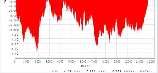
136 The global motion response, the low frequency motions for sway Figure : The global motion response, the low frequency motions for sway. The global motion response, the low frequency motions for heave Figure : The global motion response, the low frequency motions for heave. 6-24

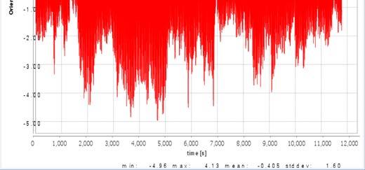
137 The global motion response, the low frequency motions for roll Figure : The global motion response, the low frequency motions for roll. The global motion response, the low frequency motions for pitch Figure : The global motion response, the low frequency motions for pitch. 6-25

138 The global motion response, the low frequency motions for yaw Figure : The global motion response, the low frequency motions for yaw. Besides, the global motion response for the total motion as combination of the low frequency motions (LF motions) and wave frequency motions (WF motions) can be found from Figure 6.18 to Figure The total global motion response, the total frequency motions for surge Figure : The total global motion response, the total frequency motions for surge. 6-26

139 The total global motion response, the total frequency motions for sway Figure : The total global motion response, the total frequency motions for sway. The total global motion response, the total frequency motions for heave Figure : The total global motion response, the total frequency motions for heave. 6-27

140 The total global motion response, the total frequency motions for roll Figure : The total global motion response, the total frequency motions for roll. The total global motion response, the total frequency motions for pitch Figure : The total global motion response, the total frequency motions for pitch. 6-28

141 The total global motion response, the total frequency motions for yaw Figure : The total global motion response, the total frequency motions for roll. B. The Horizontal Offset Values The horizontal offset can be derived from the global motion response. The summary of the global motion response for the low frequency motions and the total frequency motions can be seen in Table below: Table : The Summary of The Global Motion Response of A Cylindrical S400 Floater The Global Motion Response in Low Frequency Motions Channel Min Max Mean Std. Skewness Kurtosi Dev. s Surge XG translation LF Motion Sway YG translation LF Motion Heave ZG translation LF Motion Roll XL rotation LF Motion Pitch YL rotation LF Motion Yaw ZG rotation LF Motion The Global Motion Response in Total Frequency Motions Channel Min Max Mean Std. Skewness Kurtosi Dev. s Surge XG translation Total Motion Sway YG translation Total Motion Heave ZG translation Total Motion Roll XL rotation Total Motion Pitch YL rotation Total Motion Yaw ZG rotation Total Motion

142 Based on Table 6.14, it is clear that a cylindrical S400 floater will experience significant surge motion in LF and total frequency (LF+WF). These responses are resulting due to surge excitation from the second order force such as the mean wave (drift) forces and the slowly varying forces from waves or currents. Besides, the analysis also shows that a cylindrical S400 floater maybe particularly sensitive to total heave in total frequency motion (LF+WF). The magnitude of the values of the first order wave forces (Hs =15.6 m and Tp= 15s) should be the main reason for this result. Further, the horizontal offset of a cylindrical S400 floater for the environmental data, 100 years wind years wave + 10 years currents can be determined as follow: The wave The wind The current The static offset: The max offset : Jonswap double peaked spectrum (Hs=15.6m and Tp=15.5s) : NPD Spectrum wind : Current profile : 3,37 m : 22,82 m C. Mooring Line Dynamic Tensions The mooring line dynamic tensions of a cylindrical S400 floater have been found for the environmental data: 100 years wind years wave + 10 years currents as follow: The wave The wind The current : Jonswap double peaked spectrum (Hs=15.6m and Tp=15.5s) : NPD Spectrum wind : Current profile The summary of the mooring line dynamic tension for a cylindrical S400 floater can be seen in Table 6.15 below: Table : The Summary of Mooring Line Dynamic Tensions of a cylindrical S400 floater Channel Min Tension kn Max Tension kn Mean Tension kn Std. Dev. Skewness Kurtosis S400_Line S400_Line S400_Line S400_Line S400_Line S400_Line S400_Line S400_Line S400_Line S400_Line S400_Line S400_Line

143 While the result of mooring line dynamic tensions gives by time series for each line can be seen from Figure 6.24 to Figure 6.35 below: The mooring line dynamic tensions in time series for S400_Line1 Figure : The mooring line dynamic tensions in time series for S400_Line1. The mooring line dynamic tensions in time series for S400_Line2 Figure : The mooring line dynamic tensions in time series for S400_Line

144 The mooring line dynamic tensions in time series for S400_Line3 Figure : The mooring line dynamic tensions in time series for S400_Line3. The mooring line dynamic tensions in time series for S400_Line4 Figure : The mooring line dynamic tensions in time series for S400_Line

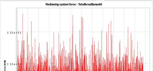
145 The mooring line dynamic tensions in time series for S400_Line5 Figure : The mooring line dynamic tensions in time series for S400_Line5. The mooring line dynamic tensions in time series for S400_Line6 Figure : The mooring line dynamic tensions in time series for S400_Line

146 The mooring line dynamic tensions in time series for S400_Line7 Figure : The mooring line dynamic tensions in time series for S400_Line7. The mooring line dynamic tensions in time series for S400_Line8 Figure : The mooring line dynamic tensions in time series for S400_Line

147 The mooring line dynamic tensions in time series for S400_Line9 Figure : The mooring line dynamic tensions in time series for S400_Line9. The mooring line dynamic tensions in time series for S400_Line10 Figure : The mooring line dynamic tensions in time series for S400_Line

148 The mooring line dynamic tensions in time series for S400_Line11 Figure : The mooring line dynamic tensions in time series for S400_Line11. The mooring line dynamic tensions in time series for S400_Line12 Figure : The mooring line dynamic tensions in time series for S400_Line

149 The forces in a mooring line will also be checked with the acceptance criteria for tension in the Ultimate Limit State (ULS) based on ISO (2005). The results can be seen in Table 6.16 below: Table : The Summary of Line Tension Limit and Design Safety Factor Channel Min Tension kn Max Tension kn Mean Tension kn Std. Dev. Skewness Kurtosis Line Tension Limit (% of MBL) Design Safety Factor S400_Line S400_Line S400_Line S400_Line S400_Line S400_Line S400_Line S400_Line S400_Line S400_Line S400_Line S400_Line Based on ISO (2005), the acceptance criteria for the tension in the Ultimate Limit State (ULS) for intact stability when using a quasi static method should be line tension limit 50% of the Minimum Breaking Load (MBL) of the mooring line component. Moreover, the specified minimum safety factor is 2.00 as defined in ISO (2005). Hence, the criteria above are met for the mooring system design for a cylindrical S400 floater. D. The Results The resulting analysis for dynamic condition such as the time series of second order wave forces and the wave drift damping forces will be also presented here. Further, these results will be compared to the result in Chapter 8 to show the influence of the hydrodynamic interaction. 1. The second order wave forces The summary of the results for the second order wave forces are described in surge, sway and yaw can be seen in Table 6.17 while the graphs can be found from Figure 6.36 to Figure Table : The Summary of Second Order Wave Forces Channel Min Tension kn Max Tension kn Mean Tension kn Std. Dev. Skewness Kurtosis XR Force (in Surge) kn 0.01 kn kn YR Force (In Sway) kn kn kn Moment ZR axis (in Yaw) 0.00 KNm 0.00 KNm 0.00 KNm

150 Figure : The second order wave forces XR Forces (in Surge). Figure : The second order wave forces YR Forces (in Sway). 6-38

151 Figure : The second order wave moment Moment ZR axis (in Yaw). 2. The wave drift damping forces The results for the wave drift damping forces are described for surge, sway and yaw. The summary can be seen in Table 6.18 while the graphs can be found from Figure 6.39 to Figure Table : The Summary of wave drift damping forces Channel Min Tension Max Tension Mean Std. kn kn Tension kn Dev. Skewness Kurtosis XR Force (in Surge) kn kn kn YR Force (In Sway) kn kn 9.77 kn Moment ZR axis (in Yaw) 0.00 KNm 0.00 KNm 0.00 KNm

152 Figure : The drift damping forces XR Forces (in Surge). Figure : The drift damping forces YR Forces (in Sway). 6-40

153 Figure : The drift damping forces moment ZR axis (in Yaw). 6-41

154 Chapter 7 1 Riser Analysis M.S.c. Thesis Coupled Dynamic Analysis of Cylindrical FPSO, Moorings and Riser Based on Numerical Simulation This chapter will present a general description of the riser system and present the riser analysis to obtain a feasible configuration for a floating offshore system. As we know, the nonlinear coupled dynamic analysis represents a truly integrated system which ensures the accurate prediction of response simultaneously for the overall system as well as the individual response of floater, moorings and risers. This is the main advantage for performing coupled analysis rather than the decoupled analysis. On the other hand, it also requires many efforts and is very time consuming since this analysis demand substantial efforts since it requires a single and complete model including a floater, moorings and riser. It also requires the detailed model for each component and characterization of the environments in covering relevant load models. Several strategies can be proposed to achieve higher efficiency analysis. In this case, the dynamic slender structure analysis for riser configuration will be performed in RIFLEX as a decoupled analysis in order to reduce time analysis. The main purpose of the analysis is to find a feasible single arbitrary configuration. The analysis will also be performed in time domain analysis under two simulation schemes, static and dynamic conditions. Moreover, the modeling concept and the steps when analysis in RIFLEX will be presented briefly. In this chapter, the analysis results will be presented such as top angle (hang off position angle), effective tension, bending radius and seabed clearance briefly in order to document the feasible configurations. Furthermore, this chapter will also explain the basic knowledge of a riser system to give the perspective for the analysis. 7-1

155 7.1 Production Riser Systems Based on American Petroleum Institute definitions, API (1998), the riser system is a key element in providing safety in all phases from drilling, completion/workover, production/injection to export. The main function of a riser is to transport fluids or gas from seabed to a host platform. Additional functions of risers according to area of application are provided as follows: Conveys fluid between the wells and the floater in production and injection risers. Export fluid from floater to pipeline for export risers. Guide drilling or workover tools and tubulars to and into the wells for drilling and workover risers. In the riser system design, the dynamic behavior of the floater at the surface will mainly govern the chosen riser type. Hence, according to the ability to cope with floater motion, DNV OS F201 (2001) has categorized the production riser system into (Figure 7.1.): Top tensioned riser Compliant riser (flexible riser) Hybrid riser being a combination of tensioned and compliant risers. Top tensioned riser Compliant riser Hybrid riser Figure : Examples of riser systems Reference : Karunakaran (2008) Besides the floater s motion, the riser system design will be governed by the floater type, water depth, design of pressure/temperature, mechanical characteristics of the riser, and environmental conditions. The riser system design drivers also include a number of factors such as, host vessel access/hang off location, field layout such as number and type of risers and mooring layout. 7-2

156 Since the base case for the study is in North Sea region and the facilities should be built to withstand very harsh weather conditions in shallow waters (approximately 170 m), the application of a flexible riser (compliant riser) will be very suitable in this floating offshore system. The flexible riser has been extensively applied in North Sea, Gulf of Mexico, Brazil and West of Africa. According to Chandwani and Larsen (1997), a flexible riser is defined as an unbonded flexible pipe designed to specific engineering requirements. Moreover, a flexible riser provides the flexibility to cope with the floater s motions. Configurations of flexible risers are formed such that they could absorb floater motions without having additional equipment e.g. heave compensation system. The design flexibility to have high dynamic resistance allows flexible riser to work in deeper waters and harsher environments. Its structure consists of concentric extruded polymer and reinforcing helical metallic layers (Figure 7.2.). As shown, each metallic and polymer layer satisfies particular strength/weight/flexibility/ containment and chemical requirements. These layers will ensure that flexible risers could accommodate high curvature, allowing ease of installation and accommodation of dynamic motion. Figure : Flexible riser Reference : Chandwani and Larsen (1997) A dynamic flexible riser system can be designed for most types of floating production structures. The system flexibility is achieved by arranging the flexible pipe in some of the basic configurations below (Figure 7.3.): 7-3

157 Figure : Standard flexible riser configurations. Reference : Karunakaran (2010) Furthermore, the riser configuration design shall be performed according to the production requirements and the site specific environmental conditions. According to Yong Bai et al (2005), some basic requirements shall be taken into account while determining the riser configurations such as the global behavior and geometry of riser, structural integrity, rigidity and continuity of riser, cross sectional properties, means of support, material and costs. 7.2 Flexible Riser Design in Shallow Water and Harsh Environments In this study, many key issues of riser system design which are related to the combination of shallow water and harsh environmental conditions will be the primary focus. These situations will give the challenges of designing the riser system and will increase the complexity of riser system design. Since the field is located in shallow water condition and also harsh environment, the application of cylindrical FPSO will give many advantages. However, it also gives real challenges for riser system design. The combination of harsh environment and limited water depth conditions leads to significant challenges in riser design: Limited water depth gives very little room between the FPSO and the seabed. This condition leads to significant impact from the environmental loading and the vessel motion itself. Another challenge comes from the configuration itself. Limited water depth leads to large vessel offset and this will govern the pliancy requirements for the two extreme configurations, the far and near conditions, in the riser design. 7-4

158 Influence of the large vessel motion and the harsh environmental loadings In deep water, the vessel motion represents a significant loading impact and it will be damped gradually along the riser length. This condition cannot happen smoothly in shallow water. Furthermore, the impact of the vessel s motion from pitch and roll will be significant in shallow water. These motions will be one of the reasons why the effective top tension becomes larger at the hang off position. Not only the effective top tension but also the angle position will be larger at the hang off position. The harsh environment also leads to a significant dynamic riser behavior. In shallow water, large drag forces from the environment will result from the combination of strong current and large waves. For small submerged weight of riser under extreme currents, potential clashing with adjacent moorings is high. Another potential problem is risk of compression forces at touchdown area (TDA). Another condition that will be a main consideration is the impact loading that generates from shock due to snapping in slack condition. Significant vessel motion, (roll and pitch motion) creates slack in one position. This stored energy releases quickly when the wave passes and snapping occurs in the riser system, generating a significant shock for the system. Influence of large vessel offset As the riser system has to absorb vessel motions, large vessel motions will have direct impact on the riser behavior. As vessel offset increases due to harsh environment, options for riser configuration become limited. Hence, a Top tensioned riser may not be applied, or conventional free hanging steel catenary riser will experience high bending moment at touchdown point. Didier Hanoge (2010) has mentioned that vessel offset has major influence on the riser configuration design. It governs the pliancy requirement and the riser system must accommodate the two extreme configurations; far and near conditions, as presented in Figure 7.4. below: Figure : The influence of vessel offset in riser design. Reference: Didier Hanoge (2010) 7-5

159 Furthermore, the deeper the water depth, the higher the offset value is. However in terms of percentage, the value will be eminent. Since the riser system will be designed according to the decoupled analysis, the distance between the vessel s centers of motions to the riser hang off will be taken as single representative offset (a conservative value) due to the vessel motions (pitch and surge). In the far case, the riser length must be long enough to avoid an over stretch that would result in an unacceptable tension, while in the near case the riser length must be short enough to avoid over bending or clashing issues Riser Configuration Selections These real challenges discussed above will represent essential information to design the optimum riser configuration for a floating offshore system in Western Isles Field. As we mention above, the dynamic response of a riser system to the environmental conditions will play the key role in selection of a feasible configuration for a riser. Hoffman et al (1991) has also mentioned about the important factors that should also be considered during the configuration selection: Interference with others, such as riser systems and moorings (design layout) Activity of other vessels in the vicinity Ease of laying and retrieval and future requirements of maintenance (future development) Inspection and worker operations It should be highlighted that the dynamic responses of a riser are strong related to the environmental loading due to the wave current combination and the interaction arising from the structural non linear behavior of the riser itself. In shallow water and harsh environmental conditions, the effects of the wave current combination are very significant in the magnitude and in the direction of fluid forces. Hence, these effects will have significant influence from hydrodynamic force coefficients, current velocity profiles and relative direction of waves and currents. A number of riser concepts offer technical and commercial advantages for shallow water and harsh environmental condition. The alternative riser concepts that can be developed for these situations are: 1. Flexible riser Most of fields with floating production around the world are associated with flexible risers. The flexible risers were specified and installed in the Encova field offshore Brazil as part of a floating production system (Machado and Dumay (1980)) then these risers have been used extensively at North Sea, Gulf of Mexico, Brazil and West of Africa. This leads to flexible riser as a proven technology especially for shallow to mid water depth. Chandwani and Larsen (1997) has also stated that the flexible riser is suitable for shallow to medium water depths (>600m). The flexible riser has the ability to accommodate high curvature and dynamic motions which results in good performance for harsh environments such as Offshore Norway. It is easy to install, retrieve, corrosion resistant and reusable. Hoffman et al (1991) also pointed out some prominent characteristics for flexible risers, such as: 7-6

160 The riser accommodates the floating platform motion and hydrodynamic loading by being flexible. In storm conditions the riser undergoes large dynamic deflections and must remain in tension throughout their response. Hence it must have high structural axial stiffness and relatively low structural bending stiffness. Besides that, it also provides small resistance to lateral disturbances caused by wave and current induced hydrodynamic loadings. And Karve et al. (1988) have also mentioned that a flexible riser offers the advantage of having inherent heave compliance in the catenary thereby greatly reducing the complexity of the riser to rig and riser to subsea interfaces. Moreover, these risers are available in continuous lengths thereby avoiding seals and makeup joints every 50 feet as required by steel risers. These risers have also relatively lower fatigue sensitivity than steel catenary risers by being flexible and can be applied in many possibility configurations such as the steep wave, steep S, lazy wave, lazy S and free hanging. 2. Steel catenary riser The Steel Catenary Riser (SCR) is one direct alternative to the flexible riser. It may be used at larger diameters, higher pressures and temperatures and also may be produced more easily. It has the capacity to be suspended in longer lengths, removing the need for mid depth buoys. These risers are cheaper than the flexible risers and also can be used in greater water depths without a disproportionate increase in cost. However, the SCRs are very sensitive to environmental loading. Large heave and surge motions from host platform due to harsh environment result in buckling issues at the touchdown point. The length of pipe between the supports changes when the host platform moves. This makes the seabed touchdown point shift, hence moving the point of maximum curvature up and down along the length of the pipe at the seabed. As a result, at the touchdown area, the pipe is subjected to maximum and almost zero curvature, making the region highly sensitive to the fatigue damage. The vortex induced vibrations due to currents in deepwater application another issue for SCR design. Hence, the SCRs could be the economical solution but these risers require good engineering studies to minimize the risks due to their potential problems in design. In shallow water riser design, the riser system must be strong enough to withstand high tension and bending moments due to the harsh environment and significant vessel motions. Comparing the two riser types above, the application of flexible riser (compliant riser) will be very suitable in this floating offshore system. A Lazy Wave riser configuration has been chosen in this project. Increasing pliancy of the system is the main reasons to modify the configuration by introducing a lazy wave with a multiple buoyancy section at the hog bend position. This riser configuration will hopefully not only be a robust solution for riser but also as an economic design. As one of the solutions to reduce the impact of the vessel s motions and the environmental loading, buoyancy modules are used to reduce overall tension at the upper region and improve the curvature at the lower region. Besides that, the buoyancy modules will create 7-7

161 the riser shape desired easier. Furthermore, the hog bend position gives positive significant effects for the response of the riser system. Other ancillary components will be used to fulfill pliancy requirements in the riser design optimization. The bending stiffeners can be used to avoid overbending and increase the curvature to acceptable levels at the hang off connection Design Parameters The design of a flexible riser system should be related to many design parameters such as environmental conditions, vessel motions and riser properties. These parameters should be well defined. The main design parameters are the choice of riser configuration, the length of the riser, the system geometry and the sizing of riser and ancillary components. The other factors that should also be considered are the hang off location, the location of touchdown point and also the position of the wells. All of these parameters should be optimized to gain a feasible riser configuration. The system design will be checked by static and dynamic analysis. In the static analysis only the static riser configuration with and without vessel offset and dynamic analysis of the entire system will be performed by combining static loads with dynamic environmental loads based on the movements of the riser at the top (far and near). The riser will be analyzed in a short term periodic condition (i.e. just after installation (at 0 years operation) without any variation of riser characteristics (e.g. the dimension and weight of the riser and the ancillary components). A. Limit State Design Criteria and Design Conditions In this analysis, the limit state design criteria will be the Ultimate Limit State (ULS) to determine the level of safety required for the riser conditions. Based on DNV, DNV OS F201 (2001), the Ultimate Limit State (ULS) requires that the riser must remain intact and avoid rupture, but not necessary be able to operate. For the operating condition this limit state corresponds to the maximum resistance to an applied loads with a 10 2 annual exceedence probability. Hence the load combination for the riser will be defined as follow: 100 years Irregular Wave (Hs=15,6 m and Tp=15,5 s) for Torsethaugen (Jonswap double peaked) 10 years currents Static offset ± 25 m At Ballast condition, draft z =16.32 m Furthermore, riser system design will cover normal operations (when the riser is filled with the operating contents). Hence, the riser will always be filled with stabilized crude (i.e. the riser will not be empty or gas filled or in the other words, not analyzed in a condition with slug). The analysis will also not cover for compartment damage in order to simplify the study. B. Sensitivity analysis A sensitivity analysis will be done to study the variation of the output results for different variations of the input data to enhance and increase the understanding of the riser system s behavior and to reduce the error possibilities. 7-8

162 Sensitivity analysis should be done with respect to: Dimension and weight of the riser Buoyancy elements Seabed friction Due to short time available for the thesis work, the sensitivity analysis will not be reported in this study. C. Load designs Yong Bai et al. (2005) have categorized the loads acting on marine risers as follows: Functional loads Loads due to the existence of the riser system without environmental and accidental effects. The following shall be considered as functional loads: 1. Weight of riser and contents 2. Pressures due to internal contents and external hydrostatics 3. Buoyancy 4. Thermal effects 5. Nominal top tension The following should be considered as appropriate: 1. Weight of marine growth, attachments, tubing contents 2. Loads due to internal contents flow, surges, slugs or pigs 3. Loads due to installation 4. Loads due to vessel restraints Environmental loads Loads caused by the surrounding environment that are not classified as functional or accidental loads. The following shall be considered as environmental loads: 1. Wave loads 2. Current loads Accidental loads Design Criterion Loads caused by the surrounding environment that are not classified as functional or accidental loads. The following shall be considered as accidental loads: 1. Partial loss of station keeping capability 2. Dropped objects 3. Riser collisions, vessel impact and operational malfunction The design of a flexible riser system is usually based on the allowable pipe curvature or MBR (Minimum Bending Radius) and allowable tensions which are prescribed by the manufacturer. These criteria will also be influenced by the clearance area between the riser and other parts of the floating offshore system. 7-9

163 The allowable curvature and the tension are based on a full scales test from the manufacturer combined with stress analysis carried out by the manufacturer and these limits ensure that the flexible pipe will not be overstressed when responding to dynamic loads and vessel motions. The system should also be designed such that the flexible pipe is always in tension throughout its dynamic response cycle. The minimum clearances are also specified to avoid clashing problems between the riser and the seabed or the riser and the vessel or the riser and mooring lines. The main requirements from the results of the analysis will be based on: A. Top angle position In this design analysis, maximum top angle positions for the design will be limited to around deg in static analysis and less than 45 deg at dynamic analysis for the Ultimate Limit State (ALS). This is to ensure that overstressing or compression will not happen along the upper location around the hang off position. B. Effective tension In this design analysis, any compression would be avoided with upper limit of 5 kn because compression may cause (birdcaging and) buckling which may affect the integrity of the riser adversely and reduce the service life. C. Bending radius Minimum bending radius (MBR) for the flexible pipe is governed by the allowable strain of the polymeric layers and the permissible relative movements of the wires in the metallic armour layers during pipe bending. Minimum bending radius (MBR) criterions are determined based on Braestrup (2005): Bending radius requirements can be seen in Table 7.1 below: Reference: Braestrup (2005) Table : Design MBR requirements MBR Design Criterion Static application 1,0 times storage MBR Dynamic application Normal operation 1,5 times storage MBR Abnormal operation 1,25 times storage MBR D. Seabed clearance and line clashing Minimum clearances are specified to avoid clashing problems between the riser and the seabed or the riser and the vessel and between the riser or other adjacent risers, the cables or the mooring systems. Seabed clearance at the sag bend position is 5 m and line clashing checks are performed. 7-10

164 7.2.4 Methodology Design and Analysis Steps In this chapter, the riser system will be analyzed by using RIFLEX for decoupled analysis in order to reduce time analysis. In the de coupled analysis, the results of simulated motions of a cylindrical S400 floater based on large body theory in WADAM will be transferred as top end excitation of the riser in order to calculate dynamic loads in these elements. Moreover, this analysis only considers the vessel motion where the wave load comes from the wave frequency loads as first order wave loads while the low frequency motion that comes from secondary order wave load such as the mean wave (drift) force and slowly varying wave force will be neglected. This analysis only depends on the vessel s Response Amplitude Operator (RAO) as input without any influence from secondary order force. Hence, there is only little integration between the cylindrical S400 floater and the riser. Further, these effects from the vessel motions and environmental loadings will be simulated in the two extreme riser configurations; far and near conditions. These far and near conditions will be represented by a representative offset value. These values should also accommodate the mean and low frequency motion (LF) since we neglect these terms of the vessel motions in this simulation. The variations of representative offset values are carried to investigate the effect on the riser based on different vessel positions. Hence, the static configuration of the riser system will be strongly influenced by the variations of the representative offset value. Generally, this value is determined by hypothetical or empirical calculations from the previous projects. Furthermore, the deeper the water depth, the higher the offset value is. However in terms of percentage, the value will be reduced with depth. Besides the water depth, the environment characteristics in the area will also influence the magnitude of the representative offset value. Further the analysis will be performed in time domain as problem solving method. Time domain analysis should be used in the riser analysis since we have to deal with non linear systems such as drag forces, finite motion and finite wave amplitude effects. The riser design is iterative and the process may continue until all the design requirements are optimum. A methodology is needed to provide a systematic design to fulfill the requirements of the global analysis. Simple steps of the riser analysis for the cylindrical S400 floater based on the decoupled analysis can be seen in Figure 7.5.: 7-11

165 Riser System Data and Assumption Design Criteria Limitation Load Combination Modeling Challenge Riser Configuration Result Modeling Design Criteria Check Modification /Adjustment No OK Sensitivity analysis Yes Final Riser Design Figure : Methodology design for a riser system. In this study, the riser system for the Western Isles Field will be modeled as a single production riser for with 6 and 8 diameter in RIFLEX. A Lazy Wave riser configuration has been chosen based on reasonable proponents discussed in subchapter As the first step in the riser system design, the data and assumptions used as input will be identified to provide all relevant situations for the design criterions and limit states. Furthermore, the data and the assumptions will be categorized as below: The field layout data Water depth and orientation of the riser and hang off coordinates of the riser can be determined from Western Isles Field layout Pipe data sheets and ancillary components Type of pipe (flexible riser), the conveyed fluid and contents data, the dimension specification for the risers (e.g. internal diameter, outside diameter, etc), the structure and limit specification (e.g. bending stiffness, axial stiffness and minimum bending radius) and the ancillary components data. The detail information about the field layout data, pipe data sheets and ancillary components can be found in Subchapter

166 The environmental data Current profile for 10 years condition, wave profile for 100 years condition and seabed friction coefficient The vessel response and the variations of a representative offset value The vessel response will be based on the first order wave forces which are described in the frequency domain as a linear motion transfer function, also denoted Response Amplitude Operator (RAO). The further details can be found in Appendix A. The vessel offset will be determined as a representative offset value by hypothetically empirical calculations. These values will accommodate mean and low frequency motion (LF). The variations of the representative offset values are carried out to investigate the effect on the riser based on different vessel positions for two extreme riser configurations; the far and near conditions. The detail information about a representative offset value can be found in Subchapter The Western Isles Field Layout and Model Properties for the Riser System A. The Western Isles Field Layout The Western Isles Field consists of two drill centers denoted North Drill Centre and South Drill Centre. Separate risers are routed to the two drill centers. However, the study will only model two risers for the South Drill Centre; for 6 and 8 production risers in RIFLEX as depicted in Figure 7.6. below: North Riser System SevanS400 Figure : The riser system for South Drill Centre. 7-13

167 Moreover, the offshore field Western Isles Field is located on shallow water conditions and also harsh environment. The water depth is approximately 170 m. The orientation of the riser system will be at 330 degrees relative Grid North. Spacing of Risers at FPSO hang off is 3.0 m both at radius 33.5 m from FPSO center. Since the analysis will be modeled in ballast loading condition (z =16.32 m), Hence the riser hang off position will be at (33.5m; 16.32m). B. Model Properties for the Riser System 1. Flexible riser properties The flexible riser properties contain the data about dimensions and weight of the riser, the structural limit prescribed from manufacture and hydrodynamic coefficients. A. Physical properties for the risers Dimension and weight of the riser will give contributions to the functional loads on the riser and the strength capability of the riser. Gudmestad (2007) has mentioned that the thickness has a linear relation to the strength capability of the riser. Higher thickness gives higher strength value. On other side, the economical reason should be the main consideration because higher thickness will spend higher resources. Optimization has to be done to get proper dimensions based on the design conditions such as pressure and mass flow. The structural limits are given by maximum tension, bending stiffness, axial tensile stiffness and minimum bending radius. As slender structures, the risers will also experience drag forces and lift forces in constant currents. The drag forces are caused by the friction between the cylinder and the fluid. These forces will be affected by the roughness of the cylinder. A rough cylinder will set up larger eddy currents and the forces will be larger. In this analysis, we are only concerned with the drag forces. On the other hand, the lift forces will be neglected because they will not have a big difference pressure between upstream and downstream. The data about dimensions and weight for risers, structural limits and also hydrodynamic coefficients can be found in Table 7.2 and Table 7.3 below: Reference: Sevan Marine (2011) Table : Physical Properties for Risers Parameter Unit 6" 8" Outer diameter mm Inner diameter mm Weight in air kg/m Bending 20 deg C knm Axial stiffness MN MBR storage m

168 Reference: Sevan Marine (2011) Table : Physical Properties for Risers Normal drag Tangential drag Normal added mass Bare line Bouyancy modules Bending stiffener The bending stiffeners are used to avoid overbending and increase the curvature to acceptable levels. It will be applied at the top position of the risers to reduce the free floating of the sag bend. In the analysis, it will be assigned as a variable parameter. 3. Buoyancy modules The analysis will include buoyancy modules in order to: Achieving stable configuration, distributed buoyancy will be used to comply the motions of the FSU without undue stress onto the flexible riser due to the environmental forces Minimizing compression and excessive bending in the touchdown region as buffer Decreasing the tension required at the surface In the analysis, buoyancy modules are distributed over specific lengths of the riser configuration and the suitable dry weight of buoyant elements will be assigned along the buoyancy section as a variable parameter Modeling Concept by RIFLEX The riser design will be modeled by using RIFLEX based on the finite element technique which has proved to be a powerful tool for several applications. Moreover, the riser will be modeled with beam elements which will be formulated by using a co rotated ghost reference description. The basic theory about this can be found in Chapter 2 based on Marintek (2010) for RIFLEX Theory Manual Finite Element Formulation. The procedure for the riser system model can be found in details in Marintek (2010) RIFLEX User Manual Finite Element Formulation. The program system consists of three programs or modules communicating by a file system as shown in Figure 7.7. below: 7-15

169 Figure : Layout of the RIFLEX program system and file communication between modules. The FREMOD and PLOMOD modules will not be used in this analysis; PLOMOD module is just a plot routine. The INPMOD module has the function to gather all data inputs and organizes a data base for use during the subsequent analyses in STAMOD. The STAMOD module has the function to perform several types of static analyses. Further these results are used to define the initial configuration for a succeeding dynamic analysis in DYNMOD module. The data for the element mesh, stressfree configuration and key data for the finite element analysis are also generated by STAMOD module based on system data given as input to INPMOD module. In the DYNMOD module, time domain dynamic analyses based on the final static configuration will be performed in order to calculate the responses of the system. The results of the simulation in time series format will be read by OUTMOD module then the plot of the time series and statistical parameters can be access from PLOMOD. The detailed information about the input to these modules as being used in the analysis can be found in Appendix D. The flexible riser that will be modeled in RIFLEX will adopt an Arbitrary Riser system configuration (AR). This system will determine the layout configuration of a riser based on its topology and boundary conditions. The system definition starts with definition of the topology and proceeds in increasing detail to the line and component descriptions. The system topology is in general described in terms of branching points and terminal points. These points are denoted supernodes. Further, these supernodes are classified as free, fixed or prescribed depending on their boundary condition modelling. 7-16

170 We use a Lazy Wave riser configuration in this project. It will use supernodes which are denoted as free or fixed. A free constrained node will be used for modeling a joint point between a bending stiffener and a body line of the riser while a fixed constrained node will be used for modeling at hangoff position and at connection to the seabed. If a supernode is denoted free, all degrees of freedom are free while in the fixed constrained node, all degrees of freedom are fixed. Besides supernodes, the initial layout configuration of a riser will also be defined as a stressfree configuration. This configuration will represent the initial and no structural forces/deformations along a riser. Furthermore, this configuration will be used as a basis for calculation of structural forces and deformations in the finite element analysis. The stressfree configuration for the Arbitrary Riser system configuration (AR) is defined by the input and can be seen in the file sima_inpmod (RES file). Further between two supernodes, the riser system will be identified as a line which contains elements. The number of elements in each segment will influence the accuracy of the result. The description of the layout configuration design in the Arbitrary Riser system configuration (AR) can be seen in Figure 7.8. below: 5 SUPERNODE LINE SEGMENT ELEMENT : Branching points or nodes with specified boundary conditions : Suspended structure between two supernodes. : (Part of) line with uniform cross section properties and element length : Finite element unit Element Figure : System definition for the description of the layout configuration design of the Arbitrary Riser system configuration (AR). Hence, the riser line in the layout configuration design of the riser will be defined as Arbitrary Riser system (AR) which has 2 supernodes and 5 segments with many elements in each segment. 7-17

171 Moreover, the riser design will be modeled by using RIFLEX in two stages: 1. Static analyses As the first stage of the modeling, the result from the static analysis will determine the acceptable system layout for the riser. In this stage, the effects of changing the design parameters (i.e. system geometry and length) on the static curvature and tension will be investigated. Based on these parameters, the design will select a suitable range of system geometries and lengths that satisfy the design criteria. Moreover, the static effects of the vessel offset (based on far and near conditions) and the current loading are investigated for different locations. The static analysis is based on a complete non linear formulation. However, the catenary theory will also be implemented to reduce the computing time as a good starting point. Static analysis comprises: Equilibrium configuration Parameter variations of tension or position parameters, current velocity and direction 2. Dynamic time domain analysis including eigen value analysis In the second stage, the dynamic analysis of the system will be performed to assess the global dynamic response. An acceptable system layout from the previous stage and the dynamic loadings will be considered here. The analysis will combine the loads from the combination of waves and current, vessel positions and riser contents in order to prove the acceptance condition based on the design criteria. The results of these analyses such as the dynamic curvatures, tensions and clearance area should be checked against the design limits. Time domain analysis is based on step by step numerical integration of the dynamic equilibrium equations. Dynamic analysis comprises: Eigenvalue analysis, natural frequencies and mode shapes Response to harmonic motion and wave excitation Response to irregular wave and motion excitation 7.3 Riser Analysis Layout and Schematic Riser Configurations The riser design is an iterative and complicated process that may continue until all the design requirements are optimum. Since the riser system design will be the focus in the combination of shallow water and harsh environmental conditions, the challenges from this condition will introduce some modifications in order to obtain a feasible riser configuration. The main challenges that will be faced in the design process come from the large vessel motion and vessel offset due to limited space between the FPSO and the seabed. The harsh environmental loading will also give impact on the dynamic riser behavior. Beside, the external influence from the environmental condition, the configuration itself will govern the pliancy requirement and the riser system should accommodate two extreme configurations, 7-18

172 the far and the near conditions. In the far case, the riser length must be long enough to avoid an over stretching that would result in an unacceptable tension, while in the near case the riser length must be short enough to avoid over bending or clashing issues. Hence, some modifications have been made as follows: Heavy weight riser By increasing the weight of the riser to reduce the free floating loads from the riser makes the configuration more stable A multiple buoyancy section at the hog bend position By introducing a lazy wave with a multiple buoyancy section at the hog bend position, this riser configuration will not only represent a robust solution for the riser but also be an economic design. As one of the solutions to reduce the impact of the vessel motion and the environmental loading, buoyancy modules are used to reduce the overall tension at the upper region and improve the curvature at the lower region. Besides that, the buoyancy modules will create the riser shape desired easier. Furthermore, the hog bend position gives significant positive effects for the response of the riser system. By referring to the design parameters, the feasible riser configurations for 6 and 8 production risers in the Western Isle field can be seen in Figure and Figure Segment 4 Segment 3 Segment 2 Segment 1 Figure : The riser configuration of the 6 production riser for the Western Isle Field. 7-19

173 The feasible configuration for the 6 production riser will adopt a Lazy Wave riser configuration with multiple buoyancy sections at the hog bend position. The upper buoyancy modules are shown by segment 3 and the lower buoyancy modules are shown by segment 2 in Figure 7.9. The upper buoyancy modules will help to reduce the overall tension at the upper region from the vessel motion and environmental loading (the combination of waves and currents) while the lower buoyancy modules will help to improve the curvature at the lower region. Hence the buoyancy modules will create the riser shape desired easier. The hog bend position influences positive significantly the response of the riser system. The tip of the hog bend will be put in range 130 m below the surface in order to minimize riser pay load on the FPSO and to obtain good dynamic response of the riser system. The weight risers itself will be heavy having a length of 320 m. The detailed information about its cross section and the buoyancy module s cross section can be found in Appendix D. As like the feasible configuration for the 6 production riser, the 8 production riser will also adopt a Lazy Wave riser configuration with multiple buoyancy sections at the hog bend position. The upper buoyancy modules are shown by segment 3 and the lower buoyancy modules are shown by segment 2 in Figure The hog bend position gives significant positive effects for the response of the riser system. The tip of the hog bend will be put at a range 120 m below the surface. The weight of the riser itself will also be heavy riser having a length 320 m. The detailed information about its cross section and the buoyancy module s cross section can be found in Appendix D. Segment 4 Segment 3 Segment 2 Segment 1 Figure : The riser configuration of the 8 production riser for the Western Isle Field. 7-20

174 The system design will be checked by static and dynamic analysis. In the static analysis only the static riser configuration with and without vessel offset will be considered while the dynamic analysis of the entire system will be performed by combining static loads with dynamic environmental loads based on movements of the riser Static Condition The purpose of the static analysis is to determine the acceptable system layout for a riser based on the input parameters. The main design parameters are such as the choice of riser configuration, the length of riser, the system geometry and the sizing of riser and ancillary components based on the consideration of the hang off location and the location for the touchdown point will be simulated in the static condition. The main requirements for the result of the analysis are such as the top angle position, effective tension, bending radius and seabed clearance and clashing. The top angle position and seabed clearance can be seen in Figure 7.9. and Figure The top angle positions in static condition are less than 15 deg while the seabed clearance in static condition are around 5 m to 15 m on the lowest point in the sag bend area. The other results such as the static forces, bending moment and bending radius can be seen below. The static forces will be represented by the effective tension, the riser itself should always be in tension because compression along the riser should be avoided as it will cause (birdcaging and) buckling which may affect the integrity of the riser adversely and reduce the service life. The bending moment and the curvature of the riser will show the performance of the riser. Furthermore, the curvature of the riser will show the capability of the riser to be bent until its limits without kinking or damaging it and it depends on its minimum bending radius. The smaller the bending radius, the greater is the material flexibility (as the radius of curvature decreases, the curvature increases). A. Effective tension The effective tensions for the 6 and 8 production risers can be seen in Figure and Figure The maximum effective tension for the 6 production riser is 180 kn while the minimum will be 32,08 kn. The range of values for the effective tension for the 8 production riser is slightly different. The maximum effective tension for the 8 production riser is 155 kn while the minimum will be 26,58 kn. These results are quite good and any compression can be avoided. 7-21

175 Figure : The static effective tension for the 6 production riser for the Western Isle Field. 7-22

176 Figure : The static effective tension for the 8 production riser for the Western Isle Field. B. Bending Moment and Curvature The bending moments for the 6 and 8 production risers can be seen in Figure and Figure while the curvatures for the 6 and 8 production risers can be seen in Figure and Figure The maximum bending moment and curvature for the 6 and 8 production risers are found in the hang off position. The results are quite good since they are still within the allowable limit. Based on the design criterion, in the static condition; the minimum bending radius (MBR) of a riser should be same or less than that of the MBR at storage. The MBR for a 6 riser is 1,76 m or in the terms of curvature this will be 0,57 (1/1,76). The MBR for a 8 riser is 2,02 m or in the terms of curvature this will be 0,5 (1/2,02). These results are quite good since the curvatures of the risers are less than 0,5 (Figure and Figure 7.16.) 7-23

177 Figure : The static bending moment for the 6 production riser for the Western Isle Field. Figure : The static bending moment for the 8 production riser for the Western Isle Field. 7-24

178 Figure : The static curvatures for the 6 production riser for the Western Isle Field. Figure : The static curvatures for the 8 production riser for the Western Isle Field. 7-25

179 7.3.3 Dynamic Condition In the dynamic condition, time domain dynamic analyses will be performed based on the final static configuration in order to calculate the global dynamic responses of the system. Furthermore, the results of these analyses such as the dynamic tensions and curvatures should be checked against the design limits. During the dynamic simulation, the feasible riser configurations for 6 and 8 production risers in the Western Isle field as shown in Figure and Figure will move in a range in a response to hydrodynamic loading. The movements of a riser will be recorded in the diagram showing the displacement envelope curvature. The diagram of the displacement envelope curvatures for the 6 and 8 production risers can be seen in Figure and Figure Figure : The displacement envelope curvature for the 6 production riser for the Western Isle Field. 7-26

180 Figure : The displacement envelope curvature for the 8 production riser for the Western Isle Field. The other results such as the dynamic tensions and curvatures can be seen below. A. Effective tension The effective tensions for the 6 and 8 production risers can be seen in Figure and Figure The maximum effective tension for the 6 production riser is 240 kn while the minimum will be 23,94 kn. The range of values for the effective tension for the 8 production riser is slightly different. The maximum effective tension for the 8 production riser is 220 kn while the minimum will be 10 kn. These results are quite good and any compression can be avoided. 7-27

181 Figure : The dynamic effective tension for the 6 production riser for the Western Isle Field. 7-28

182 Figure : The dynamic effective tension for the 8 production riser for the Western Isle Field. B. Bending Moment and Curvature The bending moments for the 6 and 8 production risers can be seen in Figure and Figure while the curvatures for the 6 and 8 production risers can be seen in Figure and Figure The maximum bending moment and curvature for 6 and 8 production risers are found in the hang off position. The results are quite good since they are still within the allowable limit. Based on the design criterion, in the dynamic condition; the minimum bending radius (MBR) of a riser should be same or less than 1,5 times that of the MBR at storage. The MBR for a 6 riser is 1,76 m or in terms of the curvature this will be 0,57 (1/1,76). Hence the limit MBR in the dynamic condition is 0,38. While, the MBR for a 8 riser is 2,02 m or in terms of the curvature this will be 0,5 (1/2,02). Hence the limit MBR in the dynamic condition is 0,33. These results are quite good since the curvatures of the risers are less than 0,3 (Figure and Figure 7.24.) 7-29

183 Figure : The dynamic bending moment for the 6 production riser for the Western Isle Field. Figure : The dynamic bending moment for the 8 production riser for the Western Isle Field. 7-30

184 Figure : The dynamic curvatures for the 6 production riser for the Western Isle Field. Figure : The dynamic curvatures for the 8 production riser for the Western Isle Field. 7-31

185 Chapter 8 1 Coupled Dynamic Analysis M.S.c. Thesis Coupled Dynamic Analysis of Cylindrical FPSO, Moorings and Riser Based on Numerical Simulation This chapter will present a single complete computer model that includes the cylindrical floater, moorings and riser with use of SIMA. In principle, SIMA will combine two nonlinear numerical simulations, a SIMO and a RIFLEX analysis. In other words, the cylindrical floater and moorings model from SIMO will be combined with an AR (arbitrary riser) configuration from RIFLEX in time domain analysis. A set of accurate predictions of the response of the overall system will be obtained because the nonlinear coupled dynamic analysis ensures a truly integrated system. Not only the accurate prediction of the response of the overall system but also the individual responses of the floater, moorings and risers are obtained. Hence, the accurate prediction of the floater motions will be presented here. The accurate prediction of the motions of the cylindrical floater will refer to the global motion response for the total motion as combinations of the low frequency motions (LF motions) and the wave frequency motions (WF motions) and will be presented here. Further, these results will be compared to the results from the global motion response for the total motion as found in Chapter 6 (Subchapter points A and B). Besides the accurate prediction of the motion of the cylindrical floater, the results from the riser analysis will also be presented here. In this chapter, the riser analysis will be performed by using the nonlinear coupled dynamic analysis in time domain under two simulation schemes, static and dynamic conditions. As for the response of the floater, the results will be compared to the results from the decoupled analysis of the top angle (hang off position angle), effective tension, bending radius and seabed clearance in Chapter 7 (Subchapters and 7.3.3). Furthermore, this chapter will also give a description of the analysis program that will be used, SIMA to give the perspective for the analysis. 8-1

186 8.1 Modeling Concept by SIMA Marintek As the final step, the cylindrical floater S400, 12 mooring lines and two of feasible riser configurations for a production riser with 6 and 8 diameter will be modeled as one complete model which is required in the nonlinear coupled dynamic analysis to obtain a consistent treatment of the coupling effect between the cylindrical FPSO and the slender members. This method will generate the solution of the nonlinear coupled dynamic analysis in time domain using a non linear integration scheme and will adopt the dynamic equilibrium equation of the spatially discredited system (Omberg, H. et al. (1997)). Further, The SIMA Marintek computer software will be used in this study because it has the capability to integrate the cylindrical floater S400, moorings and riser as one complete model. Here, a complete model of the floating offshore system will be modeled in one module of The SIMA Marintek/the RIFLEX Coupled model (combination software for RIFLEX and SIMO which are run together). In other words, a model of the cylindrical floater S400 with moorings system as established from SIMO will be combined with a model of a feasible riser system from RIFLEX into a complete model in RIFLEX Coupled and are run together in a time domain analysis. The SIMA Marintek software is developed as a Joint Industry Project by MARINTEK and Statoil. The SIMA Marintek is a powerful tool for modeling and analysis of tasks within the field of marine technology. Beside it has the capability to integrate each components of a floating offshore system, The SIMA Marintek has also the capability to support several programs that will be used in this study such as RIFLEX and SIMO. Hence, the analysis can be accessed in a single file as done in the library data system of SIMA Marintek (Figure 8.1). In the nonlinear coupled dynamic analysis, the complete model of the floating offshore system will consist of three principal structural components such as the cylindrical floater, moorings and riser responding to the environmental loading due to wind, waves and currents. Moreover, a previous model of the cylindrical floater and the mooring system from Chapters 5 and 6 will be modeled as the body while a previous feasible riser configuration model will be extracted from Chapter 7 to be modeled as an AR (arbitrary riser configuration) system. Further information about how to model the system components can be found in Chapter 4. As an integrated dynamic system, the environmental forces on the floater induce the motions which will be introduced in a detailed Finite Element Model of the moorings and risers. The finite element model has been used to describe the behavior of a given variable internal to the element in terms of the displacement (or other generalized co ordinates) by utilizing interpolation functions (van den Boom (1985)). Here, two different types of elements are introduced in the model, a 3D bar/cable element where the bending stiffness is negligible and a 3D beam element to include the bending stiffness. The bar element presents only 3 translational DOF per node and do not provide the rotational stiffness. Therefore, it will be a suitable model to represent the moorings. On the other hand, the beam element will incorporate rotational stiffness and it will be a suitable model to represent the flexible riser. Moreover, the bar element is formulated using a total 8-2

187 Lagrangian description, while the beam element formulation uses a co rotated ghost reference description. The basic theory about this can be found in Chapter 2 based on Marintek (2010) for RIFLEX Theory Manual Finite Element Formulation. The procedure for the riser system model can be found in details in Marintek (2010) RIFLEX User Manual Finite Element Formulation. Since a Finite Element Model has been applied to slender members (moorings and risers), a dynamic analysis will be performed during the design because the dynamic behavior of the slender members strongly increases the maximum line tensions and may affect the low frequency motions of the moored structure by increasing the virtual stiffness and damping of the system. Moreover, the application of the Finite Element Model will be for all system components, including the body of the cylindrical S400 floater. The FEM model of the cylindrical S400 floater (Hydro and Mass model) that originated from Wadam/HydroD will be taken as input. This input has been adopted from SIMO as a body model directly. In addition, the kinetic and radiation data will also be taken as inputs to obtain the forces that are acting on the hull. Since the model will be quite complex, a master slave approach will be used to connect the riser and the frequency dependent floater and moorings. This connection will be placed in the body section as a so called AR (arbitrary riser) Connection. Here, the environmental loading from winds, waves and currents will be considered. The study has also provided a set of wind, wave and current criteria associated with the extreme events. The criteria are considered to be independent, i.e. no account is taken of the effects of joint probability. The study will be based on the return period combination of 100 years waves and wind criteria and 10 years current criteria. The wind forces will be simulated in the time domain. The wind speed design for simulation will be taken as the average speed occurring for a period of 1 hour duration at a reference height, typically 30 ft (10m) above the mean still water level. NPD wind spectrum (ISO (2005), wind spectrum) will be used. The wind loads will be simulated in time domain, no transverse gust and no admittance function will be used. The study will analyze the wave loads by using irregular waves. The irregular waves will have contributions in describing the real condition of the surface sea. The wave data will be based to the study from Physe Ltd (2010). All year omni directional extreme significant wave heights have been assessed by using NNS (Northern North Sea) measured data set. The full NNS measured data set was used to create frequency distributions and the data were extrapolated by applying a range of functional fits. Peaks Over Threshold (POT) analysis was also performed on the time series data, picking 40, 60 and 80 storms to determine the best fit. The EVA (Extreme Value Analysis) results for extreme significant wave heights are given in Table 8.1 below: 8-3

188 Table 8.1. : The EVA Analysis Results for 100 Years Waves Reference: PhyseE Ltd (2010) Where: FT3 = Fisher Tippett distribution, Type 3, POT= Peaks Over Threshold (POT) (40, 60 and 80 storms) CFE = Cumulative Frequency Extrapolation Further, the extreme significant wave height values for return periods of 100 years were calculated from the NNS measured data. The complete NNS data set was extrapolated applying both a 10% and a 95% Weibull fit to each data set. Hence, a 100 year significant wave height design value of 15.6 m is recommended for the Western Isles location. According to Physe Ltd (2010), the final recommendations for the waves at the Western Isles location are given Table 8.2. below: Table 8.2. : Extreme Wave Height and Associated Periods Omnidirectional Reference: PhyseE Ltd (2010) Further, this waves criteria (Hs = 15,6m and Tp= 15,5s) will be modeled by the Torsethaugen Spectrum (Jonswap double peaked). It will be simulated for 3 hours + build up time in the SIMA Marintek. 8-4

189 The current criteria are based on the 10 years current criteria. The vertical current profile for the Western Isles will be calculated from Guidance Notes; Department of Energy (1990) for Offshore Installations: Guidance on Design, Construction and Certification. Further, the floating offshore system will be modeled for two conditions, the static and dynamic conditions. The calculation parameters for each condition will be set differently depending on their functions. The static condition stage has as functions to obtain a static equilibrium position and generate the initial condition for the dynamic simulation while the dynamic simulation will be performed in the dynamic condition in order to calculate the responses of the system responding to the dynamic loading conditions. Since the analysis has been performed as a time domain analysis, it requires a proper simulation length to obtain a steady result. Moreover, in the dynamic condition the environmental criteria (the wind, waves and current criteria) has been simulated for 3 hours + build up time. According to Omberg et al. (1998), the extreme values found from 3 hours + simulations will represent a reasonable max expected value for the simulated time series, in particular as we for the floater motion have that the statistical variability, in terms of coefficient of variation, is in the range of 4 5% for the model results and 2 3% for the simulations. For the member tension the variability is 3 4% for the simulations. Further the floater s response (floater motions and the horizontal offset values) and the slender member s response such as mooring line dynamic tensions as the mooring system s response and the effective tension and the bending moment and curvature as the riser s system s response will be presented in the next subchapters. These results are presented as time series which have the maximum, minimum and mean values. Furthermore, the results will be highlighted to the maximum or minimum values to show the deviation of each result. 8-5

190 Figure 8. 1 : Library data system of the SIMA Marintek. Reference: Marintek,

191 8.2 The System Response in the Nonlinear-Coupled Dynamic Analysis The main reason for performing a coupled dynamic analysis is to obtain an accurate prediction of the response, simultaneously for the overall system as well as the individual response of the floater, moorings and risers. The accurate prediction of the response for the overall system can be obtained since the coupled dynamic analysis ensures a truly integrated dynamic interaction between the components in the offshore floating system. Hence, the estimation of the mean offset and the floater motions can be generated accurately to quantify the coupling effects between the floating offshore system (the floater, moorings and riser) and the associated structural response (e.g. motion responses) for offshore structure design. Since the analysis has been performed in the time domain for problem solving, the floater motions in the time domain, the horizontal offset values and the mooring line dynamic tensions will be presented as time series results. The resulting analysis for the floater motions and the horizontal offset values will be presented in time series below: Floater Motions In the nonlinear coupled dynamic analysis, the global motion response of the cylindrical S400 floater will be represented by the total frequency motions as combinations of the low frequency motions (LF motions) and wave frequency motions (WF motions). The summary of the global motion response i.e. the total frequency motions can be seen in Table 8.3 below: Table 8.3. : The Summary of The Global Motion Response of The cylindrical S400 Floater in the Nonlinear Coupled Dynamic Analysis The Global Motion Response in Total Frequency Motions Channel Min Max Mean Std. Dev. Surge XG translation Total Motion Sway YG translation Total Motion Heave ZG translation Total Motion Roll XL rotation Total Motion Pitch YL rotation Total Motion Yaw ZG rotation Total Motion Further, the global motion response for the total motion as combinations of the low frequency motions (LF motions) and wave frequency motions (WF motions) can be found from Figure 8.2 to Figure

192 The total global motion response, the total frequency motions for surge Figure 8. 2 : The total global motion response, the total frequency motions for surge. The total global motion response, the total frequency motions for sway Figure 8. 3 : The total global motion response, the total frequency motions for sway 8-8

193 The total global motion response, the total frequency motions for heave Figure 8. 4 : The total global motion response, the total frequency motions for heave. The total global motion response, the total frequency motions for roll Figure 8. 5 : The total global motion response, the total frequency motions for roll. 8-9

194 The total global motion response, the total frequency motions for pitch Figure 8. 6 : The total global motion response, the total frequency motions for pitch. The total global motion response, the total frequency motions for yaw Figure 8. 7 : The total global motion response, the total frequency motions for yaw. 8-10