Magnuson-Stevens Fishery Conservation and Management Act Essential Fish Habitat Assessment

Transcription

1 Endangered Species Act Biological Assessment for Anadromous Salmonids, Green Sturgeon, Pacific Eulachon, Marine Mammals, & Marine Turtles and Magnuson-Stevens Fishery Conservation and Management Act Essential Fish Habitat Assessment for the Major Rehabilitation of the Jetty System at the Mouth of the Columbia River in Pacific County, Washington and Clatsop County, Oregon Prepared by U.S. Army Corps of Engineers Portland District, Portland, Oregon December 2010

2 TABLE OF CONTENTS INTRODUCTION... 1 Project Authority... 2 Consultation History... 3 Background... 3 DESCRIPTION OF THE PROPOSED ACTION... 8 Overview... 8 General Terms and Features Design Elements and Structural Features of Proposed Action MCR North Jetty MCR South Jetty MCR Jetty A Construction Measures and Implementation Activities Construction Schedule and Timing Sources and Transportation of Rock Barge Offloading Facilities Dredged Material Disposal Sites Pile Installation and Removal Rock Placement Construction Staging, Storage, and Rock Stock Piles Temporary Erosion Controls Emergency Response Hazardous Materials Spill Containment and Control Water Quality Monitoring Wetland Mitigation and Habitat Improvements Action Area ENDANGERED SPECIES ACT ENVIRONMENTAL ASSESSMENT Introduction Status of the Species and Critical Habitat Salmon and Steelhead Salmon and Steelhead Critical Habitat Eulachon Marine Mammals Marine Turtles Environmental Baseline Overview Physical Characteristics Sediment Quality Other Activities and Conditions Effects of the Action Rock Transport Construction Access, Staging, Storage, and Rock Stockpiling Rock Placement i

3 Dredging Disposal Barge Offloading Facilities Pile Installation and Removal Wetland and Lagoon Fill and Culvert Replacement Dune Augmentation Water Quality Hydraulic and Hydrological Processes Mitigation and Habitat Improvements Effects of the Action on Listed Species Listed Marine and Anadromous Fish Green Sturgeon Eulachon Marine Mammals Critical Habitat Cumulative Effects Synthesis and Integration of Effects Species at the Population Scale Critical Habitat at the Watershed Scale Conclusion MAGNUSON-STEVENS FISHERY CONSERVATION AND MANAGEMENT ACT Potential Effects of the Proposed Action on EFH Salmon EFH Coastal Pelagic EFH Groundfish EFH Determination for Essential Fish Habitat REFERENCES LIST OF FIGURES Figure 1. Location of the Jetty System at the MCR... 1 Figure 2. Rubble-mound Jetties at the MCR... 4 Figure 3. Typical Spur Cross Section - Change with Depth Figure 4. North Jetty Cross Section for Existing Condition and Scheduled Repair Template Figure 5. Proposed Action for the MCR North Jetty Figure 6. North Jetty Spur Groin NJ1C Figure 7. North Jetty Spur Groin NJ2C Figure 8. North Jetty Spur Groin NJ3O Figure 9. North Jetty Spur Groin NJ4C Figure 10. North Jetty Head Cap Figure 11. Proposed Action for the MCR South Jetty Figure 12. South Jetty Cross Section for Existing Condition and Scheduled Repair Figure 13. South Jetty Spur Groin SJ1O Figure 14. South Jetty Spur Groin SJ2C Figure 15. South Jetty Spur Groin SJ3C Figure 16. South Jetty Spur Groin SJ4C Figure 17. South Jetty Spur Groin SJ5O ii

4 Figure 18. South Jetty Head Cap Figure 19. Clatsop Spit and South Jetty Root Erosion Figure 20. South Jetty Root Shoreline Area Figure 21. Proposed Action for MCR Jetty A Figure 22. Jetty A Cross Section for Proposed Action Figure 23. Jetty A Spur Groin JA1C Figure 24. Jetty A Spur Groin JA2O Figure 25. Jetty A Head Cap Figure 26. Construction Schedule Figure 27. Potential Quarry Locations (red dots) for Repairs to MCR Jetties Figure 28. Potential Canadian Rock Source Transportation Routes Figure 29. Potential Washington Rock Source Transportation Routes Figure 30. Potential Oregon Rock Source Transportation Routes Figure 31. Potential Northern California Rock Source Transportation Routes Figure 32. Potential Railway Transportation Routes Figure 33. North Jetty Offloading, Staging, Storage and Causeway Facilities Figure 34. South Jetty Offloading, Staging, Storage and Causeway Facilities Figure 35. Jetty A Offloading, Staging, Storage and Causeway Facilities Figure 36. Cross Section of Stone Access Ramp at Barge Offloading Facilities at East End of Clatsop Spit near Parking Area D and Photos of Typical Barge Offloading Facilities Figure 37. Illustration of a Jack-up Barge Figure 38. Fast Fuel System Figure 39. Annual Monthly River Discharge at Bonneville Dam under Current Operations as Compared to Historical River Discharge with No Mainstem Dams Figure 40. Clatsop Spit Vegetative Communities (Tetra Tech 2007b) Figure 41. Sediment Trend Analysis in MCR Area Figure 42. Residual Velocity Bed Layer for August/September Time Window Figure 43. Residual Velocity Surface Layer for August/September Time Window Figure 44. Residual Velocity near North Jetty and Jetty A for August/September Time Window Figure 45. Residual Velocity near South Jetty for August/September Time Window Figure 46. Residual Velocity Bed Layer for October/November Time Window Figure 47. Residual Velocity near North Jetty and Jetty A for October/November Time Window Figure 48. Residual Velocity near South Jetty for October/November Time Window Figure 49. Mean Salinity for Bed Layer for August/September Time Window Figure 50. Mean Salinity for Surface Layer for August/September Time Window Figure 51. Mean Salinity for Surface Layer for October/November Time Window Figure 52. Mean Salinity for Surface Layer for October/November Time Window Figure 53. Bathymetry at the MCR Figure 54. Difference in Bed Level (meters) for August/September Time Window Figure 55. Difference in Bed Level (meters) for October/November Time Window Figure 56. Timing of Salmonid Life History Events in the Lower Columbia River Figure 57. Fish Presence in Lower Mainstem Columbia River below Sauvie Island (RM 87) Figure 58. Locations of Acoustic Telemetry Receiver Arrays, Figure 59. Cross-channel Distribution of Acoustic-tagged Yearling Chinook Salmon Figure 60. Cross-channel Distribution of Acoustic-tagged Steelhead Figure 61. Cross-channel Distribution of Acoustic-tagged Subyearling Chinook Salmon Figure 62. Tidal Elevations at the MCR for August/September and October/November Time Windows with Respect to Spur Groins Subjected to Periodic Submergence iii

5 LIST OF TABLES Table 1. Construction and Repair History for the MCR Jetties... 6 Table 2. Preferred Plan Design Metrics Summary for MCR Jetties Table 3. North Jetty Spur Groin Features Table 4. North Jetty Head Cap Features Table 5. North Jetty Lagoon and Wetland Fill Features Table 6. South Jetty Spur Groin Features Table 7. South Jetty Head Capping Features Table 8. Jetty A Spur Groin Feature Table 9. Jetty A Head Cap Feature Table 10. Quarry Information Table 11. Approximate Rock Volume and Area of Barge Offloading Facilities and Causeways Table 12. Estimated Dredging Volumes for Barge Offloading Facilities Table 13. Acreages Needed for Construction Staging, Storage, and Rock Stock Piles Table 14. Possible Wetland Mitigation and Habitat Improvement Features Table 15. Maximum Estimated Acreages for Habitat Improvement and Wetland Mitigation Table 16. Federal Register Notices for Final Rules that List Threatened and Endangered Species, Designate Critical Habitats, or Apply Protective Regulations to Species under Consideration Table 17. EFH Species and Potential Life Stages in the Action Area Table 18. NMFS Recovery Planning Domains and ESA-listed Salmon and Steelhead Species Table 19. Demographically Independent Salmonid Populations in the WLC Recovery Domain and Spawning Populations Table 20. LCR Chinook Salmon Populations Spawning in Oregon Table 21. UWR Chinook Salmon Populations Table 22. CR Chum Salmon Populations Spawning in Oregon Table 23. LCR Coho Salmon Populations Spawning in Oregon Table 24. LCR Steelhead Populations Spawning in Oregon Table 25. UWR Steelhead Populations Table 26. Demographically Independent Salmonid Populations in the IC Recovery Domain and Spawning Populations Table 27. SR Spring/Summer Run Chinook Salmon Populations in Oregon Table 28. MCR Steelhead Populations in Oregon Table 29. SRB Steelhead Populations in Oregon Table 30. OC Coho Salmon Populations in Oregon Table 31. SONCC Coho Salmon Populations in Oregon Table 32. PCEs of Critical Habitats Designated for ESA-listed Salmon and Steelhead Species and Corresponding Species Life History Events Table 33. PCEs of Critical Habitats Designated for SR Spring/Summer Run Chinook Salmon, SR Fall Run Chinook Salmon, SR Sockeye Salmon, SONCC Coho Salmon, and Life History Events Table 34. North Jetty Wetland Scores Table 35. Life Stages of Marine and Anadromous Species Table 36. Depths of Spur Groins with Respect to MLLW Table 37. Average Number of Pinnipeds by Month at South Jetty, Table 38. PCEs of Critical Habitats Designated for ESA-listed Salmon and Steelhead and Corresponding Life History Events Table 39. PCEs of Critical Habitats Designated for SR Spring/Summer-run Chinook Salmon, SR Fall-run Chinook Salmon, SR Sockeye Salmon, and SONCC Coho Salmon and Life History Events Table 40. PCEs of Critical Habitats Proposed for Southern Green Sturgeon and Corresponding Life History Events iv

6 INTRODUCTION The U.S. Army Corps of Engineers (Corps) prepared and is submitting this Biological Assessment (BA) to the National Marine Fisheries Service (NMFS) in compliance with the requirements of Section 7(c) of the Endangered Species Act of 1973, as amended. This BA evaluates effects to species listed on the Endangered Species Act (ESA) and their designated and proposed critical habitat, as well as an Essential Fish Habitat (EFH) analysis, in accordance with the Magnuson-Stevens Fishery Conservation and Management Act (MSA) for the Major Rehabilitation of the Jetty System at the mouth of the Columbia River (MCR). Federally listed marine and anadromous fish, mammal, and turtle species are present in the vicinity of the proposed action, as well as EFH species including five coastal pelagic species, numerous Pacific Coast groundfish species, and coho and Chinook salmon. The Corps also requests a Conference Opinion regarding effects to proposed critical habitat for leatherback turtles. Additionally, prior to construction activities, an incidental harassment authorization (IHA) for marine mammals at the South Jetty will be obtained. The Corps did not request a species list from NMFS. The Corps maintains this jetty system and navigational channels as appropriate based on necessity and appropriations. The Corps is currently proposing major repair and rehabilitation for the North Jetty, South Jetty, and Jetty A located at the MCR (Figure 1). Figure 1. Location of the Jetty System at the MCR 1

7 PROJECT AUTHORITY For the authorization for the actual construction of the MCR jetties, the present navigation channel and configuration of the inlet at the mouth of the Columbia River are the result of continuous improvement and maintenance efforts have been undertaken by the Corps Portland District since Congress has authorized the improvement of the MCR for navigation through the following legislation. Senate Executive Document 13, 47 th Congress, 2 nd Session (5 July 1884) authorized the Corps to construct the South Jetty (first 4.5 miles) for the purpose of attaining a 30-foot channel across the bar at the MCR. House Document 94, 56 th Congress, 1 st Session (3 March 1905) authorized the Corps to extend the South Jetty (to 6.62 miles) and construct a North Jetty (2.35 miles long) for the purpose of attaining a 40-foot channel (0.5 mile wide) across the bar at the MCR. House Document 249, 83 rd Congress, 2 nd Session (3 September 1954) authorized a bar channel of 48 feet in depth and a spur jetty ("B") on the north shore of the inlet. Funds for Jetty "B" construction were not appropriated. Public Law (30 July 1983) authorized the deepening of the northern most 2,000 feet of the MCR channel to a depth of 55 feet below mean lower low water (MLLW). The MCR federal navigation project was originally authorized (in 1884) before formulation of local sponsor cost sharing agreements; therefore, all navigation maintenance and improvements at MCR are borne by the Federal Government. The authority for maintenance of the MCR jetties comes from the original authority for construction of the project and then with Corps policies for the operations, maintenance, and management of a Corps project (Chapter 11 of EP ). For navigation, completed projects like the MCR have established that operations and maintenance (O&M) is solely a federal responsibility to be accomplished at federal cost. When maintaining a Corps project, there is regular O&M, major maintenance, and major rehabilitation. Major rehabilitation consists of either one or both of two mutually exclusive categories, reliability or efficiency improvements. Reliability. Rehabilitation of a major project feature that consists of structural work on a Corps operated and maintained facility to improve reliability of an existing structure, the result of which will be a deferral of capital expenditures to replace the structure. Rehabilitation will be considered as an alternative when it can significantly extend the physical life of the feature (such as a jetty) and can be economically justified by a benefit/cost relationship. Each year the budget EC delineates the dollar limits and construction seasons (usually two construction seasons). Efficiency Improvements. This category will enhance operational efficiency of major project components. Operational efficiency will increase outputs beyond the original project design. Thus, the authority for maintenance of the MCR jetties comes from the authorization documents for the project and/or the authority to operate and maintain the structures. 2

8 CONSULTATION HISTORY As the project s preferred alternative has evolved, the Corps has been coordinating with NMFS since On November 5, 2007, the Corps submitted an earlier version of this Biological Assessment (BA) proposing a larger jetty rebuilds. On January 11, 2008, the Corps provided a memo responding to inquiries NMFS had made regarding the BA. Subsequently, the BA was withdrawn later in January of 2008 due to significant changes in the project description. Regular coordination with NMFS and was reinstituted in the spring of 2010 after publication of the revised Draft Environmental Assessment in which a new proposed action with a smaller project footprint was determined to be the preferred alternative with which the Corps of Engineers would be moving forward. In August of 2010, a site visit to view construction activities on the Tillamook North Jetty was conducted with NMFS and Corps representatives in order to observe and to compare construction activities and design elements associated with a similar, smaller-scale jetty rehabilitation project. To ensure development of the updated Biological Assessment fully addressed ESA Consultation requirements and expectations, since July 2010 the Corps also has been meeting on a nearly weekly basis with NMFS to further discuss and describe proposed actions, related studies, and jetty design model runs. The Corps has determined that the proposed action will have no effect on the following species of marine turtles: loggerhead sea turtles (Caretta caretta), green sea turtles (Chelonia mydas), and olive ridley sea turtles (Lepidochelys olivacea). The Corps is also seeking a Conference Opinion regarding proposed critical habitat for leatherback sea turtles, and has determined the proposed actions may affect but are not likely to adversely affect (NLAA) leatherback sea turtles. The Corps has determined that the proposed action is not likely to adversely affect (NLAA) the following marine mammal species: blue whales (Balaenoptera musculus), fin whales (B. physalus), humpback whales (Megaptera novaeangliae), sperm whales (Physeter macrocephalus), killer whales (Orcinus orca) and sei whales (B. borealis). Previously, for interim repairs on the South Jetty, the Corps obtained an IHA permit as it was believed that sea lions would be disturbed during construction (Corps 2007). The Corps has determined that the proposed action is likely to adversely affect Stellar sea lions (Eumotopias jubatus) and will again obtain an IHA permit from NMFS for incidental harassment of Steller sea lions during construction, as well as non-federally listed California sea lions and harbor seals. Through this Biological Analysis the Corps has further determined that the proposed action may affect and is likely to adversely affect eulachon (Thaleichthys pacificus). The Corps has also determined that the proposed action is likely to adversely affect green sturgeon (Acipenser medirosris). Finally, the Corps has determined that the proposed action may affect and is likely to adversely affect all runs of listed salmonids and steelhead discussed further in this BA. BACKGROUND The MCR project consists of a 0.5-mile wide navigation channel extending for about 6 miles (3 miles seaward and shoreward of the tip of the North Jetty) through a jettied entrance between the Columbia River and the Pacific Ocean on the border between Washington and Oregon. Figure 1 shows the navigation project and the three primary navigation structures, the North Jetty, South Jetty, and Jetty A. Those structures are shown in more detail in Figure 2. The North Jetty and Jetty A are located in Pacific County, Washington, near Ilwaco and Long Beach on the Long 3

9 Beach Peninsula. The South Jetty is located in Clatsop County, Oregon near Warrenton/Hammond and Astoria. Figure 2. Rubble-mound Jetties at the MCR Top left photo shows the South Jetty looking east. The remnant feature shown disconnected from the primary structure is the concrete monolith that was constructed in The top right photo shows Jetty A. The bottom photo illustrates the North Jetty and the shoreline north of the MCR. South Jetty Jetty A North Jetty 4

10 From 1885 to 1939, three rubble-mound jetties with a total length of 9.7 miles were constructed at the MCR on massive tidal shoals. The jetties were constructed to accelerate the flow of the river, which helps maintain the depth and orientation of the navigation channel, and to provide protection for ships of all sizes (both commercial and recreational) entering and leaving the Columbia River. The intention was to secure a consistent navigation channel through the coastal inlet, though morphology of the inlet currently remains in a dynamic, high-energy state. Under such conditions, the jetties have experienced significant deterioration since construction, mainly due to extreme wave attack and foundation instability associated with erosion of the tidal shoals on which the jetties were built. The initial 4.5-mile section of the South Jetty was completed in The Rivers and Harbor Act of 3 March 1905 authorized the extension of the South Jetty to 6.6 miles, with the 2.4-mile extension completed in Historical records show that six spur groins were constructed along the channel side of the South Jetty. Four of the groins were subsequently buried by accreted shoreline or sand shoal. Nine repairs to the South Jetty have been completed with the latest one in To date, jetty rock placement at the South Jetty totals approximately 8.8 million tons. In spite of these repairs and structural features, over 6,100 feet of head loss has occurred at the South Jetty. The North Jetty was completed in Three repairs to the North Jetty have been made with the last one completed in To date, jetty rock placement totals approximately 3.4 million tons. Since initial construction, about 0.4 miles of the North Jetty head has eroded and is no longer functional. Jetty A was constructed in 1939 to 1.1 miles in length in connection with rehabilitation of the North Jetty for the purpose of channel stabilization. Its purpose was to assist in controlling the location and direction of the ebb tidal flow through the navigation entrance. Improvements made from 1930 to 1942 (including addition of Jetty A and Sand Island pile dikes) produced the present entrance configuration. The construction and repair history of the MCR jetties is summarized in Table 1. The Corps dredging and in-water disposal of dredged sediments to maintain the above referenced authorized navigation channel is conducted under the provisions of sections 102 and 103 of the Marine Protection Reserve and Sanctuaries Act of 1972, sections 401 and 404 of the Clean Water Act of 1977, and in accordance with Regulations 33 CFR parts

11 Table 1. Construction and Repair History for the MCR Jetties 1881: Proposed project to build a strong pile-dike, 3 feet high about at low tide, 8,000 feet long and 20 feet wide along a line previously established on the south side. The structure to start near the northeast corner of Fort Stevens, following the 12-foot curve, dike will be directed a little westward of the outer part of headland of Cape Hancock. It was stated that work commence soon (during summer and autumn) because channel maintenance is dependent upon building up Clatsop Spit. 1883: A jetty plan approved by the Board of Engineers from the south cape of the entrance on the spit. A survey was conducted in October-November of the south cape, Point Adams, to extreme low water. The jetty extends from Point Adams and makes the distance between the outer end of the jetty and Cape Disappointment the same as the distance between Chinook Point and Point Adams. The Board stated that any structures placed in-river should not harm the river and should keep the channel open using the tide; therefore, the jetty should not obstruct the entry of the flood tide. The jetty design called for a crest elevation at low water level. Estimated depths of various jetty sections from the landward end are: 5,000 feet - less than +6 feet; 7,500 feet +6 to +11 feet; 4,000 feet +11 to +16 feet; and 7,500 feet +16 to +21 feet. Jetty crest elevation was designed to be at low water level because of wave violence that could harm a higher jetty. The logic was that a higher jetty could be built, if needed later, by placing more stone on the existing jetty. A jetty height to mid-tide level was suggested but not recommended because the lower jetty would be quite effective in directing the ebb tide and would interfere less with the flood tide. A higher jetty would result in higher maintenance costs due to the jetty being more exposed to wave action. 1884: The improvement plan for MCR was approved by the Rivers and Harbors Act of July 5, 1884 to maintain a channel 30 feet deep at mean low tide by constructing a low-tide jetty, about 4.5 miles long, from near Fort Stevens on the South Cape to a point about 3 miles south of Cape Disappointment : Original construction South Jetty from Fort Stevens (station 25+80) across Trestle Bay and Clatsop Spit to station Rock placed with a natural slope to an elevation from 4 to 12 feet, crest width roughly 10 feet. The jetty, of a brushmattress and stone ballast, was built for 1,020 feet from ordinary highest tide-line, and minor constructions added. Material has filled along the jetty s south side, moving the shoreline seaward. Highest tide-line is located at tramway station A 115 feet long spur was built landward of the jetty for shore protection. A 510 feet long sand-catch, consisting of heavy beach drift and loose brush, was built on the south side of landward end of the jetty to continue filling the old outlet of a lagoon at extreme end of Point Adams. Jetty stone was originally dumped in ridges, but waves flattened and compacted the rocks to a width of 50 feet. The report indicated urgency to extend the jetty to prevent further deterioration of the bar channel. 1889: The South Jetty now under construction for 1.5 miles. Clatsop Spit has more material visible at low water and the river channel has a tendency towards a straight course out to sea. Tillamook Chute being closed. Sand building up south of the jetty adjacent to and in front of the mattresses as they are constructed. 1890: South Jetty construction is 3.25 miles underway. Jetty elevation at MLLW for about 3 miles miles of tramway to be constructed. Clatsop Spit building up, the outflowing waters being concentrated over the channel bar. Station considered the beginning of the jetty. The jetty mattress has advanced from stations to The jetty elevation is at MLLW to station From Station to the end of mattress work, there is about 9 feet of rock on top of the mattress. At station 65+00, there were signs of sinking and a large amount of rock was dumped in place : Extension of South Jetty. Crest elevation of jetty raised to 10 feet MLLW from stations to , and rock placed from stations to , elevation increasing in steps to 24 feet MLLW. Crest width is 25 feet and side slopes are natural slope of rock. Seaward bend in the jetty is added and called the knuckle : Original construction of North Jetty from stations 0+00 to Side slopes are 1 vertical by 1.5 horizontal (1:1.5) and crest width is 25 feet. Crest elevation varies from 15 to 32 feet : Repair South Jetty from stations to (shoreline to knuckle), side slopes 1:1.5, crest elevation 24 feet MLLW, and crest width 24 feet. This is first maintenance for South Jetty. The jetty had been flattened to about low water level. 2.2 million tons of stone placed in super-structure. The work completed in The end of jetty would unravel 300 feet or more, so a solid concrete terminal was constructed above low water level. The terminal was located 3,900 feet shoreward of the original jetty end that was completed in : Repair of South Jetty from stations to (knuckle to middle of outer segment). Two level cross section with crest elevations of 17 and 26 feet. Crest width of each level is 24 feet. Side slopes are 1:1.5 on channel side and vary from 1:1 to 1:1.75 to 1:2 on ocean side : Repair South Jetty from stations to (middle of outer segment to existing end). Similar design to repair. 6

12 Table 1 (continued). Construction and Repair History for the MCR Jetties 1936: Stone/asphalt cone-shaped terminal constructed on South Jetty from stations to Crest width of approximately 50 feet and elevation varied from 23 to 26 feet. Side slopes are 1: : Repair of North Jetty from stations to Crest elevation 26 feet and crest width 30 feet. Side slope 1:1.25 on ocean side and 1:1.5 on channel side. 1939: Original construction of Jetty A from stations to Crest width is 10 feet from beginning to station 53+00, 30 feet in width, and elevation at 20 feet from this point on. Four pile dikes completed at Sand Island. 1940: Repair of South Jetty with replacement rock in locations as needed : South Jetty repair from stations to Concrete terminal/stone foundation added. Crest elevation from 8-20 feet and crest width from feet, 10 inches. Side slopes determined by concrete terminal shape : Repair Jetty A from stations to Crest elevation to 20 feet with crest width of 40 feet : Repair 300 feet of Jetty A from stations to with a crest elevation of 20 feet, a crest width of 30 feet, and side slopes of 1: : Repair Jetty A from stations to with a crest elevation of 20 feet MLLW, a crest width of 30 feet, and side slopes of 1: : Repair of Jetty A from stations to with a crest elevation of 20 feet, a crest width of 30 feet, and side slopes of 1: : Repair of Jetty A from Stations to Crest elevation raised to 20 feet and a crest width of 20 feet from Stations to Crest width is 30 feet from Stations to : Repair Jetty A from stations to 90+50, with no repairs from Stations to Crest elevation built with a 10% grade from 20 feet to 24 feet from stations to The crest elevation was raised to 24 feet from stations to : South Jetty repair from stations to (before knuckle, current stationing). Crest elevation varies from 24 to 28 feet and crest width is 30 feet. Channel side slope 1:1.25 and ocean side slope 1:1.5. Repairs from stations to (old stationing). Elevation at station is +24 feet and then increased with a 0.5% grade up to +28 feet for the remainder of repair section. The repair centerline is located 13 feet north of the centerline of the original jetty design. The design crest width is 30 feet. North slope is 1:1.25 and south slope is 1: : South Jetty repair from stations to (beyond knuckle). Crest elevation begins at 28 feet and transitions to 25 feet for most of section. Side slopes vary from 1:1.5 to 1:2 and crest width is 40 feet (this appears to be the furthest seaward intact portion of current jetty). Repairs made from stations to (old stationing). The crest elevation is +28 feet at station 93+00, then decreases to +25 feet at station 95+00, and then continues with this elevation to end of the repairs. The crest width is 40 feet and has a slope of 1:1.5 from stations to Slope then transitions to 1:2 from stations to The centerline of the repair is 15 feet south of the trestle centerline. 1965: Repair North Jetty from stations to with a crest elevation of 24 feet and crest width is 30 feet. Side slopes vary from 1:1.5 to 1: : Repair South Jetty from stations to (segment before knuckle). Crest elevation varies from 22 to 25 feet MLLW. Crest width varies from feet and side slopes 1:1.5. Crest elevation varies from +22 feet at station to +25 feet at station (old stationing). From stations to 80+35, crest width is 30 feet and slope is 1:1.5. Centerline of repairs has 10 feet maximum variance to the north for the South Jetty control line. From stations to 93+00, centerline of repairs is the same as South Jetty control. Crest elevation +25 feet, width varies from feet, side slope is 1: : Interim repair of North Jetty (stations to 86+00). Crest elevation +25 feet with side slope of 1: : Interim repair of South Jetty (stations to ). Crest elevation +25 feet with side slope of 1: : Interim repair of South Jetty (stations to ). Crest elevation +25 feet with side slope of 1:2. 7

13 DESCRIPTION OF THE PROPOSED ACTION OVERVIEW The Corps proposes to perform modifications and repairs to the North and South Jetties and Jetty A at the MCR that would strengthen the jetty structures, extend their functional life, and maintain deep-draft navigation. Proposed actions are generally comprised of four categories applicable to each jetty: (1) engineered designs elements and features of the physical structures; (2) construction measures and implementation activities; (3) proposed 7(a)(1) habitat improvement measures and wetland mitigation actions to improve habitat for the benefit of listed species and to offset wetland fill, and (4) proposed establishment of and coordination with an Adaptive Management Team (AMT) comprised of Corps staff and representatives from appropriate Federal and State agencies. It is notable that the duration of the construction schedules is 20 years, with a 50-year operational lifetime for the MCR jetty system. Therefore, an inherent level of uncertainty exists regarding dynamic environmental conditions and actual conditions of and at each of the jetties. For this reason, in all cases where areas, weights, and volumes (tons, acres, cubic yards, etc.) or other metrics are indicated, these are best professional estimates and may vary by greater or lesser amounts within a 20% range when final designs are completed. These amounts represent Corps and staff s best professional judgments of what the range of variability could entail as the design is further developed and as on-the-ground conditions evolve over the 20-year construction schedule. The Corps maintains an active jetty monitoring and surveying program that will further inform the timing and design of the proposed action in order to facilitate efficient completion of the project and whenever possible to avoid emergency repair scenarios. (1) Design elements and structural features specific to each jetty include the following: North Jetty Scheduled repairs addressing the existing loss of cross section and the addition of engineering features designed to minimize future cross section instability are planned. The cross section repairs are primarily above MLLW, with a majority of stone placement not likely to extend beyond -5 ft below MLLW. In order to address the structural instability of the jetty cross-section, four spur groins will be added and the jetty head (western-most section) will be capped with large stone. Groins will be constructed primarily on existing relic stone and the head capping will be placed on relic as well as jetty stone that is above MLLW. The shore-side improvements that have been identified are culvert replacement and lagoon fill. These actions are designed to stop the current ongoing erosion of the jetty root. South Jetty Scheduled repairs addressing the existing loss of cross section and the addition of engineering features designed to minimize future cross section 8

14 instability are planned. The cross section repairs are primarily above MLLW, with a majority of stone placement not likely to extend beyond -5 ft below MLLW. In order to address the structural instability of the jetty cross-section, five spur groins will be added and the jetty head (western-most section) will be capped with large stone. Groins will be constructed primarily on existing relic stone and the head capping will be placed on relic as well as jetty stone that is above MLLW. Augmentation of the dune at the western shoreline extending south from the jetty root has been included in the repair plan. This action is intended to prevent the degradation of the jetty root and prevent the potential breaching of the fore dune. Jetty A Scheduled rehabilitation addressing the existing loss of cross section and the addition of engineering features designed to minimize future cross section instability are planned for Jetty A. The cross section repairs are primarily above MLLW, with a majority of stone placement not likely to extend beyond -5 ft below MLLW. In order to address the structural instability of the jetty cross-section, two spur groins will be added and the jetty head (southern most section) will be capped with large stone. The groins will be constructed primarily on existing relic stone and the head capping will be placed on relic as well as jetty stone that is above MLLW. Immediate rehabilitation with small cross section, two spur groins, and head capping. (2.) Construction measures and implementation activities for all three jetties include the following: Storage and staging areas for rock stockpiles and all associated construction and placement activities such as: roadways, parking areas, turn-outs, haul roads, weigh stations, yard area for sorting and staging actions, etc. Stone delivery from identified quarries either by barge or by truck. Possible transit routes have been identified. This also includes the construction and use of permanent barge offloading facilities and causeways with installation and removal of associated piles and dolphins. Stone placement either from land or water, which includes the construction, repair, and maintenance of a haul road on the jetty itself, crane set-up pads, and turnouts on jetty road. Placement by water could occur via the use of a jack-up barge on South Jetty, but will not occur by other means or on North Jetty to avoid impacts to crab and juvenile salmon migration. Regular dredging and disposal of infill at offloading facilities with frequency dependent on a combination of the evolving conditions at the site and expected construction scheduling and delivery. Disposal will occur at existing approved in-water sites. (3.) A suite of potential projects to provide 7(a) (1) habitat improvement and wetland mitigation actions have been identified as beneficial to listed species. Depending on further development of alternatives within this list, a specific project or combination of projects will be selected and constructed concurrently to provide environmental 9

15 benefits as portions of the proposed action are completed over time. Estimates for wetland impacts are preliminary and may be reduced when final delineations are completed; therefore wetland restoration may be less than approximations noted, but will be commensurate with impacts from construction activities. These restoration and habitat improvement measures will therefore require additional consultations, and it is anticipated that the proposed AMT will be of assistance in this process. It is anticipated that a programmatic opinion similar to SLOPES Restoration or Limit 8 may be useful to fulfill clearance requirements. Possible restoration measures could include an individual project or a combination of projects and actions such as: Excavation and creation of wetlands to restore and improve wetland functions including water quality, flood storage, and salmonid refugia. Culvert and tide gate replacements or retrofits to restore or improve fish passage and access to significant spawning, rearing, and resting habitat. Dike breaches to restore estuarine brackish intertidal shallow-water habitat for fish benefits. Beneficial uses of dredged material from MCR hopper dredge to replenish littoral cells. Invasive species removal and control and revegetation of native plants to restore ecological and food web functions that benefit fisheries. (4.) Due to the long duration of the MCR Jetty Rehabilitation schedule, the Corps proposes formation of a modified Adaptive Management Team (AMT). The Corps suggests annual meetings to discuss relevant design and construction challenges and modifications, technical data, and adaptive management practices as needed. The primary purpose of the proposed AMT and its implementation is to ensure construction, operation, and maintenance actions have no greater impacts than those described in the Biological Assessment, and that terms and conditions of the Biological Opinion are being met. This will also allow confirmation that any necessary construction or design refinements remain within the range and scope of effects described during Consultations. This forum will facilitate continued coordination and updating and allow the Corps to inform agency partners when unforeseen changes arise. Results regarding marine mammal and fish monitoring, wetland mitigation and habitat improvement monitoring, as well as water quality monitoring will also be made available to the AMT in order to fulfill reporting requirements and to address any unexpected field observations. Results of jetty monitoring surveys will also inform the AMT of the repair schedule and design refinements that become necessary as the system evolves over time. This venue will also provide greater transparency and allow opportunities for additional agency input. Final selection and design of the habitat improvement and wetland mitigation proposal will also be vetted through this forum to facilitate obtaining final environmental clearance documents for this component of the MCR proposed action. Potential principal partners include federal (National Marine Fisheries Service, U.S. Fish and Wildlife Service) and State (Washington, Oregon) resource management agencies. The strategy is designed to be consistent with the guidance provided in 65 Federal Register (FR)

16 GENERAL TERMS AND FEATURES Previously during earlier design phases of the proposed action, the U.S. Geological Survey (USGS) in Menlo Park, California assisted the Corps with evaluating potential improvements and impacts of rebuilding and repairing the lengths of the MCR jetties. The USGS efforts focused on using the Delft-3D model of the Columbia River estuary and adjacent coast (Delft3D 2006) to identify potential changes in circulation, salinity and sediment transport that could result from the offshore re-build of the three jetties. Increased jetty lengths were investigated to determine if they could provide a more sustainable jetty system over the long term. Although rebuild of the jetties is no longer proposed, Corps engineering staff has also indicated modeling results remain relevant and valid for evaluating jetty performance in the current proposed action, which caps jetty lengths in their current locations (Moritz 2010). The Corps Engineering Research and Development Center (ERDC) in Vicksburg, Mississippi was also contracted to conduct a physical model of the jetty cross-section design. The range of structural repair types addressed in the model included crest elevation and crest widths variations, side-slope variations, underwater berms, armor stone, and concrete armor unit options. Both the North Jetty and South Jetty were tested under low and high water conditions. Physical modeling results showed that the primary failure modes for the North and South jetties were high water wave attack and overtopping. These results were used to determine cross-section design options for the jetties that achieve varying levels of structure reliability. The following design components are a result of a combination of these models and other modeling and engineering staff efforts (Moritz and Moritz 2010). Each MCR jetty consists of three parts. The head is the seaward terminus and is exposed to the most severe wave action. Jetty head design is much more substantial than a typical jetty trunk section due to its increased exposure to wave attack and its critical protective function for the rest of the structure. The trunk forms the connection from jetty head to shore, retains sub-tidal shoals, and confines circulation in the navigation inlet. The root forms the connection from the jetty trunk to shore and prevents accreted landforms from migrating into the navigation channel. A spur groin is a relatively short structure (in comparison to jetty length) usually extending perpendicular from the main axis of a jetty. Spur groins are constructed: (1) on the ocean or beach side of a jetty to deflect the long-shore (rip) current and related littoral sediment away from the jetty and prevent littoral sediment from entering the navigation channel; and (2) on the channel side of a jetty to divert the tidal or river current away from the channel side toe of the jetty. Spur groins also act to reduce the scour affecting the foundation while increasing the current in the navigation channel, thus reducing the deposition in the channel. In areas where foundation scour threatens the overall stability of the MCR jetties, spur groins constructed perpendicular to the structure facilitate stabilization by the accumulation of sediment along the jetty s foundation. Each spur groin will have a crest width of about 20 feet, and will be constructed using a bedding layer (mixture of gravel and rock) that will be covered 11

17 with large stone sized for the location and exposure. Submergent spur groins that located at greater depths also typically have wider bases than shallower, emergent groins (Figure 3). Figure 3. Typical Spur Cross Section - Change with Depth Elevation (ft, MLLW) Typical Spur Cross Section - Change with Depth ft width Submergent Spur ft width Distance from Centerline (ft) Emergent Spur The ERDC analyzed the hydrodynamics and circulation patterns in the MCR entrance, as well as the potential impacts and effectiveness of placing spur groins on the jetties. This analysis was conducted with the coastal modeling system and other models to select the type, depth, and length of spur groins necessary to protect the each jetty from the processes causing increased scour (e.g., rip currents, eddies). Although the models were also evaluating a potential restoration of the jetties former lengths, proposed construction of spur groins at each jetty has not changed since modeling was completed. Therefore, Corps engineering staff has indicated that modeling results remain relevant and valid in their assessment of spur groin performance. Two potential construction methods could be used for spur groins, either land-based or marine-based depending on location. Barges or similar equipment could be used to dump the bedding layer rock into place and a clamshell would be used to place larger stone on top of the bedding rock layer in locations with sufficient water depth. This type of marine placement activity will not require installation of additional piles or dolphins. Material could also be placed using land-based equipment from on top of the jetty. Land-based construction may require a wide turnout crane placement with overexcavation down to grade as the crane walks back onto the main jetty axis. In addition, 12

18 the emergent spur groins may be used as turnouts for construction equipment. The land-based construction method could be used for all but the deepest spur groins. Head capping involves placing much larger armor stone at the terminus of the jetty where the highest degree of enforcement is necessary to withstand conditions. Enforcement could also include the use of concrete armor units (CAU). These will be fabricated off-site and then transported to the head via truck or barge. The armor stone at the head helps avoid recession and loss of length and by protecting the rest of the jetty from unraveling back towards the root. Repair and rehabilitation are two proposed approaches that specifically describe construction and stone placement actions for the cross-sections and engineered features along the trunks and roots of the jetties. The economics and design model used to select Schedule Repair as the proposed action at the North and South jetties predicts a certain number of repair actions that will be needed to avoid a breaching scenario during the 20-year construction schedule and 50-year operational lifetime of the jetties. Along certain sections of each jetty, wave cast and erosional forces have in some cases flattened the jetty prism and left a bedding of relic stone with little or only a partially complete jetty prism remaining. The Scheduled Repair approach prioritizes work on specific portions of the jetty so that sections in a greater degree of deterioration will be repaired with rock according to a programmed sequence developed as a result of regular jetty monitoring and inspections. Proposed repair alternatives involve adding limited amounts of stone to trunk, head, and root features in order to restore the damaged cross-sections back to a standard repair template. A repair action is generally triggered when the upper cross-sectional area falls below 30%-40% of its standard jetty template profile (only 30% or 40% of the current jetty structure remains; 60%-70% of the previously existing prism is gone). Then a standard repair template is implemented. For each repair action, a majority of stone placement will occur above MLLW. However, depending on conditions at specific jetty cross-sections, stone could extend deeper than -5 ft below MLLW in order to restore the reach back to the standard repair template. Therefore, repair actions could be slightly greater or smaller depending on the condition of the cross-section being repaired. Stone placement will remain mostly within the prism of the existing jetty and relic stone structures; though it is possible that wave actions and slope angles could result in a small percentage of further rock slipping off the relic slope. Proposed rehabilitation alternatives generally incorporate engineering components and rock placement along the cross-section of the entire root and trunk. The construction and placement sequence for Immediate Rehabilitation at Jetty A means stone placement activities are initiated at one end of the jetty and are completed continuously in succession without prioritization based on conditions at any particular jetty section. The proposed rehabilitation action on Jetty A is more robust than a repair action and includes a small cross section along the entire length of the jetty. Sections in a greater state of deterioration may receive a relatively larger amount of rock compared to sections with less damage. The rehabilitation cross-section template is expanded 13

19 slightly beyond the existing prism template. This generally involves stone placement that primarily fits within the existing footprint of the jetty structure or relic stone, but may extend slightly beyond the existing prism. It also generally involves the bulk of the rock placement above MLLW, though it could extend below in some sections, again depending conditions in each reach. The following discussions also mention station numbers on each jetty. These stations indicate lineal distance along the jetty relative to a fixed reference point (0+00) located at the landward-most point on the jetty root. Numbering begins at the reference point (0+00) and increases seaward such that each station number represents that distance in feet, multiplied by 100, plus the additional number of feet indicated after the station number. For instance, station would be 10,017 feet seaward from the reference point. A summary of design parameters for the preferred plan at each jetty is shown in Table 2. Table 2. Preferred Plan Design Metrics Summary for MCR Jetties Note: volumes, lengths and areas may vary by ± 20% upon final design. 14

20 DESIGN ELEMENTS AND STRUCTURAL FEATURES OF PROPOSED ACTION MCR North Jetty The proposed action for the North Jetty is Scheduled Repair and construction of engineered features including four spur groins and head capping, culvert replacement, and lagoon fill to stop erosion of the jetty root (Figures 4 and 5). The jetty head and foundation at the most exposed portion of jetty will be stabilized. North Jetty Trunk and Root The cross-section design from stations to will have a crest width of approximately 30 feet and will lie essentially within the existing jetty footprint based on the configuration of the original cross section, previous repair cross sections, and redistribution of jetty rock by wave action. About 460,000 tons (~287,500 cy) of new rock will be placed on relic armor stone, with the majority of stone placement above MLLW. About four repair events were predicted over the next 20 years. Each repair action is expected to cover a length range of up to 1,700 feet and include stone volumes in the range of 45,000 to 100,000 tons (~28,125-62,500 cy) per season. Figure 4. North Jetty Cross Section for Existing Condition and Scheduled Repair Template Scheduled Repair = Sta 80 & Inshore, 6-18 ton (mean = 12 ton) / Offshore of Sta 80, 8-24 ton (mean 16 ton) "Fix-as-Fails" Repair = Sta 80 & Inshore, 4-12 ton (mean = 8 ton) / Offshore of Sta 80, 6-18 ton (mean 12 ton) Relic Armor Stone, avg'd along entire length of jetty = 5-15 ton (mean = 10 ton) Core Stone = ton (mean = 1.5 ton) all stone has gamma=167 lb/ft3 Elevation, MLLW South North 50 Channel Side Ocean/Beach Side v:1h 1v:1.4h intermittent channel side Repair repairs 1v:1.5h 20 1v:1.5h Section Relic 1v:5h 10 MHHW = 7.5 ft MLLW Armor Stone Benson Beach 0 1v:1.5h -10 Core Stone -20 1v:1.1h Original Seabed -30 Present Seabed Scoured seabed armored with relic stone Distance from centerline, ft At the time of repair, it is expected that 60%-70% of the standard jetty template crosssection has been displaced. Therefore, each repair event will increase the degraded cross-section from 30%-40% back to 100% of the desired standard cross-section template. This means the overall added rock will essentially triple what exists immediately prior to the time of repair. This could be described as a ~300% increase 15

21 in rock relative to the existing jetty rock volume. However, this will not increase the jetty prism or footprint beyond the scope and size of the historic structure, and does not include any modification that changes the character, scope, or size of the original structure design. With placement divided into elevation zones per representative repair event, about 21,550 cy of rock will be placed above mean higher high water (MHHW). This represents 58% of the overall stone placement on these portions of the jetty and 376% change from the existing jetty prism. This means that currently only a small portion of the original profile remains in this zone and over three times as much stone must be placed compared to what presently remains. As described, above, this same concept applies characterizations about the rest of the zones. About 9,230 cy of rock will be placed between MHHW and MLLW. This represents 25% of the overall stone placement on these portions of the jetty and a 192% change from the existing jetty prism. About 6,675 cy of rock will be placed below MLLW. This represents 18% of the overall stone placement on these portions of the jetty and a 150% change from the existing jetty prism. The footprint of the trunk and root of the North Jetty will remain on relic stone and within its current jetty dimensions. North Jetty Spur Groins Three submergent spur groins will be placed on the channel side and one emergent spur groin will be placed on the ocean side of the North Jetty to stabilize the foundation (Figures 6 to 9). The approximate dimensions and other features of the spur groins are shown in Table 3. If possible, in order to avoid and minimize impacts to species and habitats, either one of the spur groins located around stations 50 or 70 may also serve a dual purpose as an offloading facility for stone delivery. This will occur at the contractor s discretion depending on channel current and wave conditions. Otherwise, a separate offloading facility will be constructed in the vicinity between these stations to take advantage of calmer waters. There is a dredge material disposal site along the North Jetty and adjacent disposal cells closest to the jetty and spur groins will be precluded from use to avoid interference with jetty construction and to ensure barge safety during disposal. Barge offloading structures and dredge activities are discussed in more detail later in this assessment. Representing rock volume estimated totals divided into elevation zones for all newly constructed spurs on the North Jetty, about 25 cy of rock will be placed above MHHW. This represents 0.1% of the overall stone placement on these portions of the North Jetty spur groins and there is very little or no existing jetty stone expected to be present within this elevation range. About 1,146 cy of rock will be placed between MHHW and MLLW. This represents 4% of the overall stone placement on these portions of the North Jetty spur groins and there is very little or no existing jetty stone expected to be present within this elevation range. About 27,760 cy of rock will be placed below MLLW. This represents 95.9% of the overall stone placement on these portions of the North Jetty spur groins and there is very little or no existing jetty stone expected to be present within this elevation range. The footprint of the North Jetty spurs will increase 16

22 from 0 acres to 1.55 acres. In the relevant figures, note that the difference in the vertical and horizontal scales causes a slight representational distortion along the axes. 17

23 Figure 5. Proposed Action for the MCR North Jetty 18

24 Table 3. North Jetty Spur Groin Features Spur Groin Features North Jetty Number of spurs on channel side 3 Number of spurs on ocean side 1 Approximate total rock volume per spur (+/- 20%) Approximate total rock volume (all spurs) (+/- 20%) Approximate area affected by each spur Approximate total area affected (all spurs) Approximate area of spurs above MLLW Approximate area of spurs below -20 MLLW Approximate dimension of spurs: length x width x height (feet) NJ1C: 3,350 tons (~2,094 cy) NJ2C: 11,090 tons (~6,931 cy) NJ3O: 2,010 tons (~1,256 cy) NJ4C: 29,250 tons (~18,281 cy) 53,000 tons (~33,125 cy) NJ1C: 0.18 acres NJ2C: 0.45 acres NJ3O: 0.11 acres NJ4C: 0.80 acres NJ1C: 0% NJ2C: 0% NJ3O: 24% NJ4C: 0% NJ1C: 0% NJ2C: 88% NJ3O: 0% NJ4C: 100% 1.55 acres NJ1C: 100 x 80 x 10 NJ2C: 170 x 115 x 19 NJ3O: 60 x 80 x 10 NJ4C: 170 x 115 x 19 19

25 Figure 6. North Jetty Spur Groin NJ1C Note difference in scale between vertical and horizontal axes MTL ~ +3 ft 0 8 ft - 5 ft -10 Elevation (ft, NAVD) ft width Distance from Centerline (ft) North Jetty Proposed Spur Groin - NJ1C - Channelside Elevation (ft, NAVD) Crest Length = 70 ft (from jetty toe) Effective Length = 100 ft Average Depth = ft Crest Elevation = -5 ft Average Height = 10 ft Estimated Volume = 3350 tons Estimated Bottom Area = 0.18 acres Percent above water = 0% Percent below -20 ft = 0% MHHW MLLW 100 ft -5 crest elevation survey Original Foundation Scheduled Repair Template 70 ft Average Spur Depth = ft Distance from Centerline (ft) 20

26 Figure 7. North Jetty Spur Groin NJ2C Note difference in scale between vertical and horizontal axes MTL ~ +3 ft Elevation (ft, NAVD) ft - 15 ft 110 ft width Distance from Centerline (ft) North Jetty Proposed Spur Groin NJ2C - Channelside Elevation (ft, NAVD) Crest Length = 120 ft (from jetty toe) Effective Length = 170 ft Average Depth = -34 ft Crest Elevation = -15 ft Average Height = 19 ft Estimated Volume = tons Estimated Area = 0.45 acres Percent above water = 0% Percent below -20 ft = 88% 170 ft -15 ft crest elevation 2006 Survey Original Foundation Scheduled Repair Template MHHW MLLW 120 ft Average Spur Depth = -34 ft Distance from Centerline (ft) 21

27 Figure 8. North Jetty Spur Groin NJ3O Note difference in scale between vertical and horizontal axes MTL ~ +3 ft 5 ft + 8 ft 0 Elevation (ft, NAVD) ft width Distance from Centerline (ft) North Jetty Proposed Spur Groin NJ3O - Oceanside Crest Length = 40 ft (from jetty toe) Effective Length = 60 ft Average Depth = -2 ft Crest Elevation = +8 ft Average Height = 10 ft Estimated Volume = 2010 tons Estimated Area = 0.11 acres Percent above water = 24% Percent below -20 ft = 0% ft +8 ft crest elevation 40 ft MHHW MLLW Elevation (ft, NAVD) Average Spur Depth = -2 ft survey Original Foundation Scheduled Repair Template Distance from Centerline (ft) 22

28 Figure 9. North Jetty Spur Groin NJ4C Note difference in scale between vertical and horizontal axes MTL ~ +3 ft 0 Elevation (ft, NAVD) ft - 35 ft ft width Distance from Centerline (ft) North Jetty Proposed Spur Groin NJ4C - Channelside Elevation (ft, NAVD) 35 Crest Length = 200 ft (from jetty toe) 2006 survey 30 Effective Length = 250 ft Original Foundation 25 Average Depth = -60 ft Scheduled Repair Template 20 Crest Elevation = -35 ft 15 Average Height = 25 ft MHHW 10 Estimated Volume = tons 5 Estimated Area = 0.80 acres MLLW Percent above water = 0% 0 Percent below -20 ft = 100% ft ft crest elevation ft Average Spur Depth = -60 ft Distance from Centerline (ft) 23

29 North Jetty Head Capping An armor stone cap or concrete armor units (CAU) will be placed on the head of the North Jetty to stop its deterioration (Table 4 and Figure 10). Approximately 38,000 tons (~23,750 cy) of stone or functionally equivalent CAUs will be placed on the relic stone to cap the jetty head. Future physical modeling will refine head capping features. Table 4. North Jetty Head Cap Features Head Cap Features North Jetty Location of cap stations 99 to 101 Timing of construction 2015 Approximate dimensions of cap: length x width x height (feet) 350 x 270 x 45 (2.17 acres) Stone size 30 to 50 tons Area affected (outside relic stone) None % of cap constructed on relic stone 100% Construction method Cranes set on the jetty For capping of the head, when stone placement is divided into elevation zones about 13,425 cy of rock will be placed above MHHW. This represents 49% of the overall stone placement on this portion of the jetty, and there is very little or no existing mounded jetty stone expected to be present within this elevation range. About 6,490 cy of rock will be placed between MHHW and MLLW. This represents 24% of the overall stone placement on this portion of the North Jetty, and there is very little or no existing jetty stone expected to be present within this elevation range. About 7,280 cy of rock will be placed below MLLW. This represents 27% of the overall stone placement on this portion of the North Jetty head, and a 2684% change from the existing jetty prism on this portion, as there is very little or no existing mounded jetty stone expected to be present within this elevation range. In all zones, all proposed stone placement will occur on existing base relic stone that formed the original jetty cross-section and was displaced and flattened by wave action, and does not include any modification that changes the character or increases the scope, or size of the original structure design. The terminus of the head is simply closer to shore on a shorter jetty structure. The footprint of the existing jetty mound on the flattened relic stone is approximately 1.37 acres, and the additional capping on the relic stone increases the width of the prism approximately 0.80 acres, for a total footprint of 2.17 acres, all of which will remain on the existing relic stone. 24

30 Figure 10. North Jetty Head Cap MCR North Jetty Nominal Cross Section for Existing HEAD Condition STA 104 and Proposed Head Rehab = NH1 concrete armor units: 10 to -10 ft MLLW = ton (mean = 20 ton), or sized as needed to resist wave action NH2 Stone: -10 to -20 ft MLLW = ton (mean = 32 ton), also use NH2 Stone in place of NH1 CAUs IF stone and placement is allowable Ballast Relic Stone = ton (mean = 5 ton) all stone has gamma=167 lb/ft3 Elevation, MLLW South North Channel Side Ocean/Beach Side v:2.5h 1v:2.5h Benson 10 MHHW = 7.5 ft MLLW 1v:3.0h NH2 1v:3.0h Beach 0-10 Ballast -20 Relic Armor Stone -30 Original Seabed -40 Scoured seabed armored with relic stone Present Seabed Distance from centerline, ft North Jetty Lagoon and Wetland Fill and Culvert Replacement Approximately 109,000 tons (~68,125 cy) of gravel and sand will be added to the jetty s beach side as lagoon fill to eliminate the tidal flow through the jetty that is destabilizing the foundation. A recent berm repair action now precludes lagoon inundation by tidal waters. Scouring has taken place on the north side of the North Jetty resulting in formation of a backwater area (lagoon) that was previously inundated both by tidal waters that come through the jetty and by freshwater that drains from the O Neil Lake-McKenzie Head Lagoon and wetland complex area through the accreted land to the north of the jetty and North Jetty Road. This area drains through a culvert under the road and provides some of the freshwater flow to the lagoon. The surrounding lagoon resembles a scoured-out tidal channel and is a non-vegetated (and 25

31 non-wetland) area of bare sand comprising approximately 4.71 acres. These wetland and waters will be filled to protect and stabilize the foundation of the North Jetty and to serve as a location for rock stockpiles and construction staging activities. The features of this work are shown in Table 5. Table 5. North Jetty Lagoon and Wetland Fill Features Features North Jetty Timing of construction 2014 Material used for fill Sand, gravel, quarry stone Short-term and long-term use Stockpile area, long-term stabilization of root De-watering Culvert feeding into area will be re-placed Impact on wetlands 1.78 acres Impact on Section 404 waters 4.71 acres After further hydraulic and hydrologic design, the aging culvert draining south from the wetland complex north of the roadway will be replaced, as it provides required drainage under the roadway. The design of the inlet, elevation, and culvert size will be determined so that hydrologic function in the adjacent wetland system is not negatively impacted. The outlet channel downstream of the culvert will not be filled. This area may provide an opportunity for minor stream and bank enhancement which will be evaluated when the culvert design is finalized, but this is uncertain until possible benefits can be further assessed. Under the proposed action, the existing channel will outlet to an engineered sump area comprised of newly placed lagoon fill material. In addition to infiltration through the jetty structure, this small portion of the creek currently connects the wetland to the lagoon and likely also receives some backwater flow from jetty infiltration. The current culvert is perched, and the regularly disconnected nature of the lagoon system does not appear to support anadromous fish use. Fish surveys were not completed for the stream inlet leading into this wetland complex and creek. The Corps proposes to conduct an initial sampling survey during peak juvenile salmon outmigration to determine whether or not fish salvage and fish exclusion efforts for listed species is warranted. The Corps will coordinate with NMFS if listed species are identified. Redesign of this system may provide an opportunity to accommodate improved hydrology to newly created wetlands excavated adjacent to the existing wetland complex. This will be further investigated during the hydraulic/hydrologic design analysis. 26

32 MCR South Jetty The proposed action for the South Jetty includes scheduled repairs addressing mostly above MLLW water structural instability, five spur groins, head capping, and improving the jetty shoreline near the root (Figure 11). Seven Scheduled Repair events over the next 20 years were predicted at the South Jetty. South Jetty Trunk and Root The cross-section design from stations to will have a crest width of approximately 30 feet and will lie essentially within the existing jetty footprint based on the configuration of the original cross section, previous repair cross sections, and redistribution of jetty rock by wave action (Figure 12). The majority of the stone placement will be conducted above the MLLW. Each repair action is expected to cover a length up to 2,100 feet and include stone volumes in the range of 30,000 to 118,000 tons per season (18,750-73,750 cy). As with the North Jetty repair action, it is expected that 60%-70% of the South Jetty s overall standard jetty template cross section has been displaced. Therefore, each repair event will increase the existing degraded cross section from 30%-40% back to 100% of the desired standard cross-section template. This means overall, the added rock will essentially triple what exists immediately prior to the time of repair. This could be described as a ~300% increase in rock relative to the existing jetty rock volume. However, this will not result in an increase the jetty prism or footprint beyond the scope and size of the historic structure, and does not include any modification that changes the character, scope, or size of the original structure design. Per repair event, when divided into elevation zones, about 37,640 cy of rock will be placed above MHHW. This represents 68% of the overall stone placement on these portions of the South Jetty and a 1023% change from the existing jetty prism, as very little stone currently remains in the zone and a larger amount of stone must be placed compared to what presently remains. As described, above, this same concept applies characterizations about the rest of the zones. About 10,420 cy of rock will be placed between MHHW and MLLW. This represents 19% of the overall stone placement on these portions of the South Jetty and a 225% change from the existing jetty prism. About 6,940 cy of rock will be placed below MLLW. This represents 13% of the overall stone placement on these portions of the South Jetty and a 150% change from the existing jetty cross section. However, in all zones, all proposed stone placement will occur on existing base relic stone that formed the original jetty cross section. The footprint of the trunk and root of the South Jetty will remain within its current jetty dimensions and on relic stone. 27

33 Figure 11. Proposed Action for the MCR South Jetty 28

34 Figure 12. South Jetty Cross Section for Existing Condition and Scheduled Repair and Interim Repair Template Scheduled Repair = Sta 215 & Inshore, 6-21 ton (mean = 14 ton) / Between Sta 215 & Sta 250, 7-24 ton (mean 16 ton) / Offshore of Sta 250, 7-33 ton (mean 22 ton) "Fix-as-Fails = Sta 215 & Inshore, 4-18 ton (mean = 12 ton) / Between Sta 215 & Sta 250, 6-21 ton (mean 14 ton) / Offshore of Sta 250, 6-27 ton (mean 18 ton) South Relic Armor Stone = 5-15 ton (mean = 10 ton) Core Stone = ton (mean = 4 ton) all stone has gamma=167 lb/ft3 North Ocean Side 3v:1h 1v:1h Channel Side Elevation, MLLW v:50h to 40 ft depth Present Seabed 1v:5.5h MHHW = 7.5 ft MLLW Relic Armor Stone 1v:2h Repair Section 1v:9.5h Core Stone Original Seabed 1v:2h intermittent channel side repairs 1v:1.5h 1v:1.8h Distance from centerline, ft South Jetty Spur Groins Three emergent and two submergent spur groins will be constructed to stabilize the jetty s foundation (Figures 13 to 17). The dimensions and other features of the spur groins are shown in Table 6. Representing estimated rock volume totals divided into elevation zones for all spurs on the South Jetty, about 21 cy of rock will be placed above MHHW. This represents 0.1% % of the overall stone placement on these portions of the South Jetty, and there is very little or no existing jetty stone expected to be present within this elevation range. About 2,190 cy of rock will be placed between MHHW and MLLW. This represents 12.3% of the overall stone placement on these portions of the South Jetty, and there is very little or no existing jetty stone expected to be present within this elevation range. About 15,700 cy of rock will be placed below MLLW. This represents 87.6% of the overall stone placement on these portions of the South Jetty, and there is very little or no existing jetty stone expected to be present within this elevation range. The footprint of the spurs on the South Jetty will increase from 0 acres to 1.10 acres. In the relevant figures, note that the difference in the vertical and horizontal scales causes a slight representational distortion. 29

35 Table 6. South Jetty Spur Groin Features Spur Groin Feature South Jetty Number of spurs on channel side or downstream 3 Number of spurs on ocean side or upstream 2 Approximate total rock volume per spur (+/- 20%) Approximate total rock volume (all spurs) (+/- 20%) SJ1O: 1,680 tons (~1,050 cy) SJ2C: 2,350 tons (~1,469 cy) SJ3C: 2,350 tons (~1,469 cy) SJ4C: 3,180 tons (~1,988 cy) SJ5O: 18,750 tons (~11,719 cy) 25,000 tons (~15,625 cy) Approximate area affected by each spur Approximate total area affected (all spurs) Approximate area of spurs above water Approximate area of spurs below -20 MLLW Approximate dimension of spurs: length x width x height (feet) SJ1O: 0.11 acres SJ2C: 0.13 acres SJ3C: 0.13 acres SJ4C: 0.19 acres SJ5O: 0.55 acres SJ1O: 29% SJ2C: 7% SJ3C: 7% SJ4C: 0% SJ5O: 0% SJ1O: 0% SJ2C: 0% SJ3C: 0% SJ4C: 0% SJ5O: 92% 1.10 acres SJ1O: 60 x 80 x 9 SJ2C: 70 x 80 x 10 SJ3C: 70 x 80 x 10 SJ4C: 90 x 90 x 12 SJ5O: 190 x 125 x 22 30

36 Figure 13. South Jetty Spur Groin SJ1O Note difference in scale between vertical and horizontal axes MTL ~ +3 ft 5 ft + 8 ft 0 Elevation (ft, NAVD) ft width Distance from Centerline (ft) South Jetty Proposed Spur Groin - SJ1O - Oceanside Crest Length = 40 ft (from jetty toe) Effective Length = 60 ft Average Depth = -1 ft Crest Elevation = +8 ft Average Height = 9 ft Estimated Volume = 1676 tons Estimated Area = 0.11 acres Percent above water = 29% Percent below -20 ft = 0% Elevation (ft, NAVD) 60 ft +8 ft crest elevation 40 ft MHHW 2006 survey Original Foundation Scheduled Repair Template 0 Average Spur Depth = -1 ft MLLW Distance from Centerline (ft) 31

37 Figure 14. South Jetty Spur Groin SJ2C Note difference in scale between vertical and horizontal axes MTL ~ +3 ft 2 ft + 5 ft 0 Elevation (ft, NAVD) ft width Distance from Centerline (ft) South Jetty Proposed Spur Groin SJ2C - Channelside 35 Crest Length = 45 ft (from jetty toe) Effective Length = 70 ft Average Depth = -4.5 ft Crest Elevation = +5 ft Average Height = 10 ft Estimated Volume = 2350 tons Estimated Area = 0.13 acres Percent above water = 7% Percent below -20 ft = 0% Survey Original Foundation Depth Scheduled Repair Template 70 ft Elevation (ft, NAVD) ft crest 45 ft MHHW MLLW Average Spur Depth = -4.5 ft Distance from Centerline (ft) 32

38 Figure 15. South Jetty Spur Groin SJ3C Note difference in scale between vertical and horizontal axes MTL ~ +3 ft 2 ft + 5 ft 0-10 Elevation (ft, NAVD) ft width Distance from Centerline (ft) South Jetty Proposed Spur Groin SJ3C - Channelside Crest Length = 45 ft Effective Length = 70 ft Average Depth = -5 ft Crest Elevation = +5 ft Average Height = 10 ft Estimated Volume = 2350 tons Estimated Area = 0.13 acres Percent above water = 7% Percent below -20 ft = 0% survey Original Foundation Scheduled Repair Template 70 ft Elevation (ft, NAVD) ft crest 45 ft MHHW MLLW Average Spur Depth = -5 ft Distance from Centerline (ft) 33

39 Figure 16. South Jetty Spur Groin SJ4C Note difference in scale between vertical and horizontal axes MTL ~ +3 ft 3 ft 0 ft -10 Elevation (ft, NAVD) ft width Distance from Centerline (ft) South Jetty Proposed Spur Groin SJ4C - Channelside 40 Crest Length = 60 ft (from jetty toe) Effective Length = 90 ft Average Depth = ft Crest Elevation = +0 ft Average Height = 12 ft Estimated Volume = 3180 tons Estimated Area = 0.19 acres Percent above water = 0% Percent below -20 ft = 0% survey Original Foundation Scheduled Repair Template MHHW 90 ft 0 ft crest elevation MLLW 60 ft Average Spur Depth = ft

40 Figure 17. South Jetty Spur Groin SJ5O Note difference in scale between vertical and horizontal axes MTL ~ +3 ft Elevation (ft, NAVD) ft - 15 ft 125 ft width Distance from Centerline (ft) South Jetty Proposed Spur Groin SJ5O - Oceanside Crest Length = 140 ft (from jetty toe) Effective Length = 180 ft Average Depth = -37 ft Crest Elevation = -15 ft Average Height = 22 ft Estimated Volume = tons Estimated Area = 0.55 acres Percent above water = 0% Percent below -20 ft = 92% Spur Section Original Foundation Scheduled Repair Template MHHW 190 ft 0 MLLW -15 ft crest elevation ft Average Spur Depth = -37 ft

41 South Jetty Head Capping An armor stone cap with approximately 40,000 to 74,000 tons (~25,000-46,250 cy) of stone or equivalent concrete armor units will be placed on the head of the South Jetty to stop its deterioration (Figure 18). The features of this work are shown in Table 7. For capping of the head, divided into elevation zones about 13,425 cy of rock will be placed above MHHW. This represents 52% of the overall stone placement on this portion of the South Jetty and there is very little or no existing jetty stone expected to be present within this elevation range. About 6,490 cy of rock will be placed between MHHW and MLLW. This represents 25% of the overall stone placement on this portion of the South Jetty and there is very little or no existing jetty stone expected to be present within this elevation range. About 6,050 cy of rock will be placed below MLLW. This represents 23% of the overall stone placement on this portion of the South Jetty and 1150% change from the existing base condition as there is very little or no existing mounded jetty stone expected to be present within this elevation range. In all zones, all proposed stone placement will occur on existing base relic stone that formed the original jetty cross section and was displaced and flattened by wave action, and does not include any modification that changes the character or increases the scope or size of the original structure design. The terminus of the head is simply closer to shore on a shorter jetty structure. The footprint of the existing jetty mound on the flattened relic stone is approximately 1.69 acres, and the additional capping on the relic stone increases the width of the prism approximately 0.64 acres, for a total footprint of 2.33 acres, all of which will occur on existing relic stone. Table 7. South Jetty Head Capping Features Capping Feature South Jetty Location of cap stations 311 to 313 Timing of construction Dimensions of cap: length x width x height (feet) 350 x 290 x 45 (2.33 acres) Stone size 30 to 50 tons Area affected (outside relic stone) None % of cap constructed on relic stone 100% Construction method Land-based cranes or jack-up barge 36

42 Figure 18. South Jetty Head Cap = SH1 concrete armor units: 10 to -10 ft MLLW = ton (mean = 25 ton), or sized as needed to resist wave action SH2 Stone: -10 to -20 ft MLLW = ton (mean = 32 ton), also use SH2 Stone in place of SH1 CAUs IF stone & placement is possible all stone has gamma=167 lb/ft3 Elevation, MLLW South North Ocean/Beach Side Channel Side 1v:3h 20 1v:3h 10 1v:2.5h SH2 1v:2.5h MHHW = 7.5 ft MLLW 0-10 Present Present -20 Seabed Seabed Re-worked relic armor -30 Relic Armor Stone stone Original Seabed Distance from centerline, ft South Jetty Root Erosion and Dune Augmentation Currently, the coastal shore interface along the South Jetty is in a condition of advanced deterioration (Figure 19). The foredune separating the ocean from the backshore is almost breached. The backshore is a narrow strip of a low-elevation, accretion area that separates Trestle Bay from the ocean by hundreds of yards. The offshore area along the South Jetty (and to the south) continues to erode, promoting larger wave action to affect the shoreline along the South Jetty root. The back dune of Trestle Bay has continued to advance westward due to increased circulation in the bay, seasonal wave chop, and hydraulic surcharging. Under existing conditions, the shoreline at the root of the South Jetty will continue to erode and recede, resulting in a possible shoreline breach into Trestle Bay in about 8-16 years. If this sand spit breach occurs, the result would be catastrophic. The MCR inlet would establish a secondary flow way from the estuary to the ocean along this area (south of South Jetty). This condition would profoundly disrupt navigation at the MCR and bring lasting changes to the physical nature of the inlet. 37

43 Figure 19. Clatsop Spit and South Jetty Root Erosion About 40,000 to 70,000 cy of cobble in the shape of angular or rounded graded stone is proposed at the South Jetty root in order to fortify the toe of the foredune and to improve the foreshore fronting to resist wave-induced erosion/recession (Figure 20). Maximum crest width of the template is estimated to extend 70 feet seaward from the seaward base of the present foredune. Construction of the berm augmentation would require 2 to 6 weeks. To adequately protect the foredune during storm conditions, this requires that the top of the stone berm (crest) extend vertically to approximately 25 feet NAVD and have an alongshore application length of approximately 1,100 feet, extending southward from the South Jetty root. This is equivalent to about 3 acres. The constructed template crest would be 10 to 15 feet above the current beach grade and have a 1 vertical to 10 horizontal slope aspects from crest to existing grade. Cobble is not expected to extend below MHHW. An additional layer of sand may be placed over this berm, or natural accretion may facilitate sand recruitment after construction of the adjacent spur groin. Cobble material would be procured from upland sources and placed using haul trucks and dozers. The material would be transported on existing surface roads and through Fort Stevens State Park to a beach access point at the project site. There is an existing relic access road along the jetty root that will be refurbished and used to transport stone to the dune augmentation area. Though there is an existing razor clam bed adjacent to the vicinity of the proposed dune augmentation, species impacts are not expected because all of the stone placement will occur above MHHW, and haul traffic will be precluded using Parking Lot B and from driving on the beach during material delivery. Excavator and bulldozer work will be mostly confined to the dry sand areas to further avoid negative species effects. 38

44 Figure 20. South Jetty Root Shoreline Area A Clatsop Spit N South Jetty Trestle Bay 1 Clatsop Beach 2 Pacific Ocean 2003 MCR South Jetty root, south side where Clatsop Spit joins with Clatsop Plains/Beach. Panels A and B show the erosion embayment along the south jetty root for 2003 (high tide) and 2007 (low tide). The embayment & adjacent shore have receded 40 ft landward during , reducing the protective foredune along the embayment. B Clatsop Spit N South Jetty Trestle Bay 1 2 Clatsop Beach baseline 2007 Panel C shows cross-sections 1 and 2 for 2007(shown in panels A & B). Severe erosion in this area had threatened the inlet stability during early 1930s, when jetty rehabilitation and sand augmentation measures were implemented. Erosion has again become chronic since the late 1970s. The foredune protects the backshore (elevation ft NAVD) from wave surge action during storms. If the foredune is breached, the backshore will be rapidly eroded. Without erosion abatement, it is estimated that that the Pacific Ocean will establish hydraulic connectivity with Trestle Bay in years from 2009, and again threaten inlet stability. Panel C shows two options for protecting the foredune within the erosion embayment: A SAND berm template requires ~225,000 cy of sand placement, and a COBBLE berm template requires ~60,000 cy of cobble placement. Elevation, ft, NAVD C Repair Templates for South Jetty Foredune and Berm Based on the Likely Range in Materials Used X-section 2 foredune X-section ft South of South Jetty ft South of South Jetty Sand Berm Template Cobble Berm Template Toward ocean Distance, ft, from Baseline Backshore The dune augmentation may require maintenance every 4-10 years (assume 40% replacement volume). Consideration will be given to development of revegetation plans which incorporate native dune grasses to supplement foredune stabilization in the augmentation area. This bioengineering component could help restore habitat and take advantage of natural plant rooting functions that provide greater protection from erosive forces. 39

45 MCR Jetty A The proposed action for Jetty A includes Immediate Rehabilitation with a small cross section, two spur groins, and head capping (Figure 21). Jetty A Trunk and Root The cross-section design from stations to will have a crest width of approximately 40 feet and will lie mostly within the existing jetty footprint based on the configuration of the original cross section, previous repair cross sections, and redistribution of jetty rock by wave action (Figure 22). About 55,000 tons (~34,375 cy) of new rock will be placed on the existing jetty cross section and relic armor stone on the estuary/channel side of the jetty and 75,000 tons (~46,875 cy) of new rock on the ocean side of the jetty. Though most of the work will occur above MLLW, there will also be some stone placement below this elevation. The small cross-section also has a higher likelihood of expanding beyond the relic base compared to repair actions. About 63,700 cy of rock will be placed above MHHW. This represents 63% of the overall stone placement on these portions of Jetty A and a 2020% change from the existing jetty prism, as very little stone currently remains in the zone and a larger amount of stone must be placed compared to what presently remains. As described previously for North and South jetties, this same concept applies to characterizations about the rest of the zones. About 28,940 cy of rock will be placed between MHHW and MLLW. This represents 29% of the overall stone placement on these portions of Jetty A and a 280% change from the jetty prism. About 8,030 cy of rock will be placed below MLLW. This represents 8% of the overall rock on these portions of Jetty A and a 233% change from the existing jetty prism. In all zones, most of the proposed stone placement will occur on existing base relic stone that formed the original jetty crosssection. However, the footprint of the proposed prism could increase in width compared to the existing prism by up to 10 feet along the length of the jetty (though it would still be on the relic stone). This equals about 1.2 acres, but it is not expected to result in additional habitat conversion because it will be in a bottom location already comprised of jetty stone, and does not include any modification that changes the character, scope, or size of the original structure design. 40

46 Figure 21. Proposed Action for MCR Jetty A 41

47 Figure 22. Jetty A Cross Section for Proposed Action AB1 = 9-22 tons (15 ton) Relic Armor Stone = 5-10 ton (mean = 8 ton) Core Stone = ton (mean = 1 ton) all stone has gamma=167 lb/ft3 East West Esturay Side Re-worked relic armor stone Ocean Side Elevation, MLLW Relic Stone / Shoal Original Seabed 1v:2h Relic Armor Stone 1v:1h Core Stone AB1 1v:2.5h Distance from centerline, ft 1v:2h Scoured seabed armored with relic stone MHHW = 7.5 ft MLLW Present Seabed Jetty A Spur Groins One submergent spur groin will be placed on the downstream (referred to as JA1C) side and one submergent spur groin will be placed on the upstream (referred to as JA2O) side to stabilize the jetty s foundation (Figures 23-24). The dimensions and other features of the spur groins are shown in Table 8. Representing estimated rock volume totals divided into elevation zones for all spurs on Jetty A, no stone will be placed above MLLW, and there is very little to no existing jetty stone expected to be present within either of these elevation ranges. About 10,800 cy of rock will be placed below MLLW and represents 100% of the overall stone placement on these portions of Jetty A. The footprint of the Jetty A spurs will increase from 0 acres to ~ 0.61 acres beyond existing relic stone. In the relevant figures, note that the difference in the vertical and horizontal scales causes a slight representational distortion. Table 8. Jetty A Spur Groin Feature Spur Groin Feature Jetty A Number of spurs on channel side or downstream for Jetty A 1 Number of spurs on ocean side or upstream for Jetty A 1 Approximate total rock volume per spur (+/- 20%) JA1C: 9,650 tons (~ 6,031 cy) JA2O: 7,330 tons (~ 4,581 cy) Approximate total rock volume (all spurs) (+/- 20%) 25,000 tons (~ 15,625 cy) Approximate area affected by each spur JA1C: 0.33 acres; JA2O: 0.29 acres Approximate total area affected (all spurs) 0.61 acres Approximate area of spurs above water JA1C: 0%; JA2O: 0% Approximate area of spurs below -20 MLLW JA1C: 1%; JA2O: 0% Approximate dimension of spurs: length x width x height (ft) JA1C: 135 x 105 x 18 JA2O: 125 x 100 x 15 42

48 Figure 23. Jetty A Spur Groin JA1C Note difference in scale between vertical and horizontal axes MTL ~ +3 ft 0 8 ft - 5 ft -10 Elevation (ft, NAVD) ft width Distance from Centerline (ft) Jetty A Proposed Spur Groin JA1C - Channelside 40 Crest Length = 95 ft (from jetty toe) Effective Length = 135 ft Average Depth = ft Crest Elevation = -5 ft Average Height = 18 ft Estimated Volume East= 9650 tons Estimated Area = 0.33 acres Percent above water = 0% Percent below -20 ft = 1% survey Original Foundation Rehabilitation Template West/Ocean Elevation (ft, NAVD) 135 ft -5 ft crest elevation - 8 ft MHHW MLLW ft Average Depth = ft Distance from Centerline (ft) 43

49 Figure 24. Jetty A Spur Groin JA2O Note difference in scale between vertical and horizontal axes MTL ~ +3 ft 0 8 ft - 5 ft -10 Elevation (ft, NAVD) ft width Distance from Centerline (ft) Jetty A Proposed Spur Groin JA2O - Oceanside 40 East 30 West/Ocean ft MHHW MLLW ft crest elevation Elevation (ft, NAVD) Average Depth = -20 ft ft survey -60 Original Foundation Rehabilitation Template Distance from Centerline (ft) 44

50 Jetty A Head Capping An armor stone cap of approximately 24,000 tons (~ 15,000 cy) or equivalent concrete armor units will be placed on the head of the Jetty A to stop its deterioration (Figure 21). The features of this work are shown in Table 9. For capping of the head, divided into elevation zones about 7,920 cy of rock will be placed above MHHW. This represents 44% of the overall stone placement on this portion of Jetty A and there is very little or no existing jetty stone expected to be present within this elevation range. About 4,740 cy of rock will be placed between MHHW and MLLW. This represents a 26% of the overall stone placement on this portion of Jetty A and there is very little or no existing jetty stone expected to be present within this elevation range. About 5,420 cy of rock will be placed below MLLW. This represents 30% of the overall stone placement on this portion of Jetty A and a 1783% change from the existing jetty prism, as there is very little or no existing mounded jetty stone expected to be present within this elevation range. In all zones, all proposed stone placement will occur on existing base relic stone that formed the original jetty cross-section and was displaced and flattened by wave action, and does not include any modification that changes the character or increases the scope or size of the original structure design. The terminus of the head is simply closer to shore on a shorter jetty structure.. The footprint of the existing jetty mound on the flattened relic stone is approximately 0.64 acres, and the additional capping on the relic stone increases the width of the prism approximately 0.09 acres, for a total footprint of 0.73 acres on the existing relic stone. Table 9. Jetty A Head Cap Feature Features Jetty A Location of cap stations 91 to 93 Timing of construction 2015 Dimensions of cap: length x width x height (feet) 200 x 160 x 40 (0.73 acres) Stone size 30 to 40 tons Area affected (outside relic stone) None % of cap constructed on relic stone 100% Construction method Land-based crane 45

51 Figure 25. Jetty A Head Cap = AH1 Stone: 10 to -10 ft MLLW = ton (mean = 25 ton), or sized as needed to resist wave action AH2 Stone: -10 to -20 ft MLLW = ton (mean = 20 ton) Ballast Stone = ton (mean = 5 ton) all stone has gamma=167 lb/ft3 30 East West 20 Estuary Ocean Elevation, MLLW MHHW = 7.5 ft MLLW 1v:2.0h AH2 Re-work Relic Armor Stone Original Seabed 1v:2.0h AH1 1v:1.5h -30 Scoured seabed armored with relic stone Distance from centerline, ft 46

52 CONSTRUCTION MEASURES AND IMPLEMENTATION ACTIVITIES Construction Schedule and Timing The preferred in-water work window for the Columbia River estuary at the mouth is 1 November to 28 February. However, seasonal inclement weather and sea conditions preclude safe, in-water working conditions during this timeframe. Therefore, it is likely that most of in-water work for constructing spur groins, head capping, cross-section repairs, constructing off-loading facilities, etc. will occur outside this period during calmer seas, mostly between April and October. Most landward work on the jetties will be occurring from 1 April to 15 October. Work is assumed to occur 1 June to 15 October on the more exposed sections of the jetties. Placement work may extend beyond these windows if weather and wave conditions are conducive to safe construction and delivery. Stone delivery by land or water could occur year-round, depending on delivery location and weather breaks. Barge delivery would most likely occur during the months of April through October or at other times of the year depending on breaks in the weather and which jetty is being used. Quarrying of the rock may be limited to the months of April through October depending on the regulations pertinent to each quarry. Work elements fall into four general categories for scheduling: (1) rock procurement, quarrying, and delivery transport, (2) construction site preparation, (3) lagoon fill and dune augmentations, and (4) jetty repair and rehabilitation work with construction of the design features including head capping and spur groins. Site preparation would consist of the preparation of the rock stockpile storage and staging areas, as well as the construction of any barge-offloading facilities that may be required. Approximate transport quantities by method are 30 tons per truck and 6,500 tons per barge. The majority of the jetty rehabilitation work is expected to be conducted from the top of the jetty downward using an excavator or a crane. Areas which may require marine plant work include construction at the jetty heads and some of the deeper spur groins. For design and cost-benefit estimates, the project was modeled and designed for a 50-year operational lifespan. The schedule shown in Figure 26 illustrates construction actions related to building engineered features anticipated to occur at any one or some combination of all three of the jetties for the duration of 20 years. It also includes a predicted schedule of repair actions that the Corps model estimates will be necessary within that same time period. Additional repairs have also been predicted to occur after the initial 20-year construction schedule and within the 50-year lifespan of the project. Additional repairs beyond the 20-year schedule will be similar in scale and nature to those described above in the standard repair template. Repair actions are generally triggered when a cross-section of the jetty falls below about 30%-40% of the standard repair template profile. The schedule described further in the narrative is a combined reflection of constructing specific engineered features and forecasting needed repairs. Real-time implementation of repair actions will likely vary based on evolving conditions at the jetties and could be shifted within and beyond this 20-year construction schedule. In the construction schedule, rock production and stockpiling material begins in The first jetty installation is scheduled for late spring 2014 and continues through The estimate assumes the work will be accomplished with multi-year contracts. 47

53 Figure 26. Construction Schedule Mouth of the Columbia River Jetty System Rehabilitation - Selected Plan (Construction Schedule: Jetty stone placement, existing stone re-work, engr. features) Includes stone tonnage associated with North Jetty root stabilization (lagoon fill) and jetty spur-groins for North Jetty, South Jetty, and Jetty A North Jetty - Scheduled REPAIRS South Jetty - scheduled REPAIRS Jetty A - Immediate REHAB plan = lagoon fill (North Jetty) = Jetty spur-groins Tons of Stone (1000 tons) Construction Year Mouth of the Columbia River Jetty System Rehabilitation - Selected Plan (Construction Schedule: For stone placement on Jetties and existing stone re-work) North Jetty - Scheduled REPAIRS South Jetty - scheduled REPAIRS Jetty A - Immediate REHAB plan Does NOT include stone tonnage associated with North Jetty root stabilization (lagoon fill) and jetty spur-groins for North Jetty, South Jetty, and Jetty A Tons of Stone (1000 tons) Construction Year 48

54 Due to pinniped use at the South Jetty, the Corps proposes to conduct monitoring per conditions in the expected IHA permit. The Corps anticipates that the new IHA permit will entail requirements similar to those in the previous permit. These previous requirements included monitoring and reporting the number of sea lions and seals (by species if possible) present on the South Jetty for 1 week before (re)starting work on this jetty. During construction, the Corps provided weekly reports to the NMFS, which included a summary of the previous week s numbers of sea lions and seals that may have been disturbed as a result of the jetty repair construction activities. These reports included dates, time, tidal height, maximum number of sea lions and seals on the jetty and any observed disturbances. The Corps also included a description of construction activities at the time of observation. Post-construction monitoring occurred with one count every 4 weeks for 8 weeks, to determine recolonization of the south jetty. The Corp anticipates future monitoring and reporting requirements will be similar and will designate a biologically trained on-site marine mammal observer(s) to carry out this monitoring and reporting. The Corps will submit the required reports to the NMFS and the AMT. The Oregon Department of Fish and Wildlife, who monitors sea lion use of the South Jetty, will also be apprised of the Corps work and results of the monitoring efforts. Conservation Measures the Corps will implement in order to minimize disturbance to Stellar sea lions includes the following; during land-based rock placement, the contractor vehicles and personnel will avoid as much as possible direct approach towards pinnipeds that are hauled out. If it is absolutely necessary for the contractor to make movements towards pinnipeds, the contractor shall approach in a slow and steady manner to reduce the behavioral harassment to the animals as much as possible. Monitoring and reporting will occur as required. Construction Sequence and General Schedule Rock procurement activities will be initiated for the North Jetty repair in In 2014, the onsite work will begin with filling the lagoon area behind the North Jetty root (stations 20 to 60) and installing a culvert to divert overland flow to another area that will not impact the North Jetty root stability. The lagoon area will be filled with rock, gravel, and sand. Once the lagoon is filled, the filled portion will serve as a staging and stockpile area for the rock delivered to the North Jetty site. To control further head recession of the North Jetty, in 2014 construction will focus on reconstructing the jetty head (station 88 to 99). This work will require haul road construction on top of the jetty from station 70 out to the head requiring approximately 31,000 tons of rock. The North Jetty will require installing a barge offloading facility on the channel side of the jetty at approximately station Dredging of 30,000 cy is anticipated to provide the minimum 25-ft working clearance. Concurrently, work will begin on Jetty A beginning with constructing the off-loading facility, 60,000 cy of dredging to accommodate the rock delivery by barge, and constructing the jetty crest haul road from station to Total new stone consists of approximately 50,000 tons of imported rock, equivalent to 1,700 trucks or 8 barges. In 2015 construction will continue on the North Jetty head from station 99 to 101 and installation of one spur groin at station 50 on the channel side. The haul road will need to be reworked with approximately 26,000 tons of new topping material. Work will occur concurrently with Jetty A beginning with 60,000 cy of dredging, completion of the jetty crest haul road from station 80 to 93, and installation of two spur groins. Total new stone for 2015 would consist of approximately 49

55 160,000 tons of imported rock, equivalent to 5,400 trucks or 25 barges. Work on Jetty A shall be completed this year. In 2016, work continues on the North Jetty with placement of 36,000 tons of large armor near the head at station 80 to 88. This requires refurbishing the haul road and building vehicle turnouts. In addition, three spur groins will be installed at station 70-C, 80-O, and 90-C with a total of 50,000 tons of new stone. Total new stone would consist of approximately 86,000 tons of imported rock, equivalent to 2,900 trucks or 13 barges. Site preparation work and stockpiling stone at the South Jetty will occur to prepare staging and stockpile areas for 2017 construction. In 2017, construction on the South Jetty is projected to begin, starting with construction work near the head from stations 173 to 176 and 180 to 195. South Jetty construction will require either a haul road be constructed on top of the jetty or constructed from a marine plant in order to get out to the head. Total work effort in 2017 is projected to consist of approximately 74,000 tons of rock; equivalent to 2,500 trucks or 12 barges. Work continues on the South Jetty for the next 3 years working towards the head in 2018 with a total of 86,000 tons of new armor at station 290 to 311. Head construction begins in 2019 with 30,00 tons of new head armor and installation of 4 spur groins at stations 165 O, 210-C, 230-C, and 265-C for a total of 9,000 tons of spur groin rock. The South Jetty head completes in 2020 with 44,000 tons of new stone. In 2022, construction is projected to occur concurrently on the North and South jetties: (1) continuation of North Jetty stone placement station 40 to 45 and station 65 to 73; and (2) continuation of stone placement on the South Jetty station 160 to 163, station 170 to 173, station 176 to 180, and station 195 to 200. Total rock tonnage for 2022 is estimated at 115,000 tons, equivalent to 3,850 trucks or 18 barges. In 2023, construction continues on the South Jetty with the placement of approximately 118,000 tons of rock between stations 205 to 250. The haul road will need to be reworked with approximately 62,000 tons of quarry stone road base and topping material. Total jetty stone rock tonnage to be placed would require 4,000 trucks or 18 barge loads. In 2024, construction continues on the South Jetty with the placement of approximately 76,000 tons of rock between stations 270 to 290. Total rock tonnage to be placed would require 2,600 trucks or 12 barge loads. In 2026, construction resumes on the North Jetty with the placement of approximately 52,000 tons of rock between stations 20 to 30. The long time frame from the previous construction on the North Jetty will also require rebuilding the jetty haul road from station 20 to 30. Total rock tonnage to be placed would require 1,800 trucks or 8 barge loads. In 2030, construction is projected to occur on the North and South jetties: (1) continuation of North Jetty stone placement station 30 to 40; and (2) continuation of stone placement on the South Jetty station 223 to 237, and station 250 to 253. Total rock tonnage to be placed is estimated at 129,000 tons, equivalent to 4,300 trucks or 20 barges. 50

56 In 2031, construction is projected to occur on the North and South jetties: (1) continuation of North Jetty stone placement station 88 to 99; and (2) continuation of stone placement on the South Jetty station 253 to 270. The North Jetty haul road will need to be re-built from station 65 to 99 and will require 30,000 tons of quarry waste material. Total armor stone rock tonnage to be placed is estimated at 135,000 tons, equivalent to 4,500 trucks or 21 barges. In 2032, construction continues on the South Jetty with the placement of approximately 85,000 tons of rock between stations 295 to 311. Total rock tonnage to be placed would require 2,850 trucks or 13 barge loads. The offloading facility will be removed and scheduled construction will be complete for the South Jetty. The final anticipated year of North Jetty rehabilitation is projected for 2033 with construction from stations 80 to 88. Total rock tonnage estimated is 63,000 tons, equivalent to 2,100 trucks or 10 barge loads. The offloading facility will be removed and scheduled construction will be complete for the North Jetty. Because construction at the North and South jetties is spaced out from 2014 through 2033 with intermittent work, dredging at the barge offloading sites will only be required prior to a year of actual rock delivery in preparation for upcoming construction work. The Jetty A barge offloading site will only require dredging to make that site accessible for 2 years. Dredging will only be needed if the clearance depth at the barge offloading site is not found to be adequate prior to rock delivery activities. Sources and Transportation of Rock Rock Quarries and Transport Currently, it is not exactly known where jetty rock will come from and how it will be transported to the jetty sites. However, one or more of the options discussed below would be employed (Figures 27 to 32 and Table 10). Stone sources located within 150 miles of a jetty are likely to be transported by truck directly to the jetty. Stone sources located at further distances, especially if they are located near waterways, are likely to be transported by truck to a barge onloading facility, then transported by tug and barge to either a Government-provided or commercial barge offloading site located nearby. Railway may also be an option for transporting stone, provided that an onloading site is convenient to the quarry. Most railroads follow main highway arterials, such as Interstate 5. The closest railroad terminal to the MCR South Jetty is at Tongue Point, east of Astoria, Oregon, which is about 15 miles from the jetty. The nearest railroad terminal to the MCR on the north side of the Columbia River is at Longview, Washington. The Corps intends to use operating quarries rather than opening any new quarries. The Contractor and quarry owner/operator will be responsible for ensuring that quarries selected for use are appropriately permitted and in environmental compliance with all State and Federal laws. 51

57 Canadian Quarries. Quarries in British Columbia are typically located adjacent to waterways and rock produced from these quarries will likely have a limited truck haul. Due to the long distance to the MCR, plus the immediate availability to deep water, rock would likely be loaded onto barges and shipped down the Washington Coast to barge offloading sites. Washington Quarries. Quarries located in northern Washington are typically not on the water, but are generally located within 50 miles of a potential barge on-loading site. As a result, rock would need to be hauled, at least initially, by truck. Rock would be transported by trucks most likely to a barge on-loading facility or possibly all the way to the staging site at the jetty. In the event of a combination of trucking and barging, trucks would be loaded at the quarry, and then traverse public roads to existing facilities. Once the rock is loaded on barges, it would be transported down the coast to barge offloading sites. It also is possible that railway systems may be used to transport rock much of the way to the jetties. Burlington Northern Railroad operates a rail system that parallels Interstate 5 throughout Washington which would be the most likely route rock would be transported. Rock from the quarry would be taken by truck to a nearby railway station where they would be loaded onto railway cars and transported to an intermediate staging area. Trucks would then again take the rock the remainder of the way to the jetty staging areas. Truck hauling of rock from northern Washington sources to the North Jetty or Jetty A most likely would be transported by public road to Interstate 5 or any of the main roads over to Highway 101. Trucks using Interstate 5 would either turn at Longview on Highway 4 to Highway 101, or cross over the Longview Bridge to Highway 30 near Rainier, Oregon. From this point they would proceed west to Astoria to Highway 101, crossing the Astoria-Megler Bridge through Ilwaco to the jetty staging areas. Delivery to the South Jetty most likely would use main roads to Interstate 5 or any of the main roads over to Highway 101. Trucks using Highway 101 south through Washington would likely cross the Astoria-Megler Bridge, go through Warrenton using local roads into Fort Stevens State Park and the staging area. Trucks utilizing Interstate 5 would either turn at Longview on Highway 4 to Highway 101, or on Highway 30 near Rainier, proceeding through Astoria to Highway 101, going through Warrenton through local roads into Fort Stevens State Park and the jetty staging area. Rock located within southern Washington would likely be trucked to the jetty staging areas. An exception to this would be a quarry that occurs within just a few miles of a port on the Washington Coast or a quarry that is near the Columbia River. In either of these two barge possibilities, rock would be delivered by truck to a barge on-loading facility, loaded on oceangoing or riverine barges, and delivered to one of the barge offloading facilities (see section on barge offloading facilities below). Truck hauling of rock from this area to the jetties would be as described above. 52

58 Oregon Quarries. Rock located in northern Oregon within 50 miles of the North Jetty and Jetty A would likely utilize any of the main roads over to Highway 101 or Highway 30. From this point they would cross the Astoria-Megler Bridge and proceed west through Ilwaco to the jetty staging areas. Quarries exceeding 50 miles from the jetties would likely utilize main roads at a farther distance from the jetty sites. This would involve longer haul distances on Highways 101, 30, 26, and others before crossing the Astoria-Megler Bridge and proceeding to the staging areas. Truck hauling of rock from quarries within 50 miles of the South Jetty will most likely utilize any of the main roads over to Highway 101 or Highway 30. From this point they would proceed through Astoria and Warrenton, or Seaside and Gearhart to local roads leading to Fort Stevens State Park and the jetty staging areas. Quarries exceeding 50 miles from the jetty would likely utilize main roads at a farther distance from the jetty site. This would involve longer haul distances on Highways 101, 30, 26, and others before going through Astoria and Warrenton, or Seaside and Gearhart to local roads leading into Fort Stevens State Park and the staging areas. The likely mode of transportation from southern Oregon quarries is trucking, or a combination of trucking and barging. Many of the quarries may be near the Oregon Coast; however, they may not be near a port facility that has barge on-loading capability. Providing that barge facilities are available, rock located south of Waldport would be loaded at the quarry onto trucks and traverse main public roads to the barge on-loading site, loaded on ocean-going barges, and shipped up the Oregon Coast to one of the barge offloading facilities (see section on barge offloading facilities below). Quarries north of Waldport would most likely be hauled by truck the entire distance. Southern Oregon rock sources requiring trucking would be loaded onto lowboy trucks one to three at a time and would traverse main roads to more main arterials such as Highway 101 or, to a lesser degree, Interstate 5. An effort would be made to use the least distance possible to transport the rock without sacrificing transport time. California Quarries. For northern California quarries, there would be a very long haul distance required to get rock to the jetty repair areas. Barging of rock would be the only economically feasible option. Rock would be transferred by truck from the quarries along main roads leading to Highway 101 to a barge offloading facility. 53

59 Figure 27. Potential Quarry Locations (red dots) for Repairs to MCR Jetties See corresponding quarry information located in Table

60 Table 10. Quarry Information See Figure 27 for site map. No. Quarry County and State Nearest City Road Miles from MCR Unit Weight (pcf) Reserves Available (tons) Likely Transportation Method Nearest Barge Facility 1 Columbia Granite Quarry Thurston, WA Vail, WA M Truck N/A 2 Beaver Lake Quarry Skagit, WA Clear Lake, WA M Truck, then Barge Anacortes, WA 3 Texada Quarry BC, CANADA Texada Island, BC M Barge Onsite 4 Stave Lake Quarry BC, CANADA Mission, BC M Truck, then Barge Mission, BC, Canada 5 192nd Street Quarry Clark, WA Camas, WA M Truck/Barge Camas, WA 6 Iron Mountain Quarry Snohomish, WA Granite Falls, WA Unknown Truck N/A 7 Marble Mount Quarry Skagit, WA Concrete, WA M Truck, then Barge Anacortes, WA 8 Youngs River Falls Quarry Clatsop, OR Astoria, OR M+ Truck N/A 9 Liscomb Hill Quarry Humboldt, CA Willow Creek, CA M Truck, then Barge Eureka, CA 10 Baker Creek Quarry Coos, OR Powers, OR Unknown Truck, then Barge Coos Bay, OR 11 Phipps Quarry Cowlitz, WA Castle Rock, WA M Truck N/A 12 Cox Station Quarry BC, CANADA Abbotsford, BC M Barge Onsite 13 Ekset Quarry BC, CANADA Mission, BC M Truck, then Barge Mission, BC, Canada 14 Fisher Quarry Clark, WA Camas, WA M Barge Camas, WA 15 Bankus Quarry Curry, OR Brookings, OR & M Truck, then Barge Crescent City, CA 55

61 Figure 28. Potential Canadian Rock Source Transportation Routes 56

62 Figure 29. Potential Washington Rock Source Transportation Routes 57

63 Figure 30. Potential Oregon Rock Source Transportation Routes 58

64 Figure 31. Potential Northern California Rock Source Transportation Routes 59

65 Figure 32. Potential Railway Transportation Routes For water-based delivery of rock, a tow boat and barge would deliver the rock to the channel side of the jetties where water depth, waves, and current conditions permit. During rock offloading, the barge may be secured to approximately 4 to 8 temporary dolphins/h-piles to be constructed within 200 feet of the jetty. Rock would be off-loaded from the barge by a land- or water-based crane and either placed directly within the jetty work area or stock piled on the jetty crest for subsequent placement at a later time. 60

66 For land-based delivery of rock, jetty access for rock hauling trucks would be via an existing paved road to the Benson Beach parking lot at Cape Disappointment State Park (North Jetty) and via an existing paved road to the Parking Lots C and D at the South Jetty. An existing overland route between Jetty A and North Jetty may also be used for land-based hauling. Work areas for delivery of rock, maneuvering of equipment, and stockpiling of rock near the jetties have been identified and are shown in Figures Barge Offloading Facilities Stone delivery by water could require up to four barge offloading facilities that allow ships to unload cargo onto the jetty so that it can then be placed or stockpiled for later sorting and placement. The range of locations for these facilities is shown in Figures Depending on site-specific circumstances, offloading facilities may be converted to spur groins, may be partially removed and rebuilt, may be permanently removed, or may remain as permanent facilities upon project completion. Facility removal will depend on access needs and evolving hydraulic, wave, and jetty cross-section conditions at each offloading locations. Facilities will range from approximately 200- to 500-ft long and 20- to 50-ft wide, which ranges from about 0.48 to 2.41 acres in total area. For initial construction of all four facilities combined, approximately up to 96 Z- or H-piles could be installed as dolphins, and up to 373 sections of Z- or H-piles to retain rock fill. Figure 36 shows a cross section diagram for stone access ramp at potential barge offloading facilities and photos illustrating typical barge offloading facilities. Facilities will have a 15-ft NGVD crest elevation and will be installed at channel depths between -20 and -30 NGVD. A vibratory hammer will be used for pile installation and only untreated wood will be used, where applicable. Removal and replacement of the facilities could occur within the duration of the construction schedule. Volume and acreage of fill for these facilities are shown in Table 11. Table 11. Approximate Rock Volume and Area of Barge Offloading Facilities and Causeways Location Approximate Length (ft) Approximate Rock Volume (cy) Below 0 MLLW Total Approximate Rock Volume (cy) Approximate Square Feet North Jetty 200 7,778 29,640 cy 21, Jetty A near head 200 7,778 29,640 cy 21, Jetty A mid-section causeway ,888 38, , South Jetty Parking Area D ,417 33,688 cy 47, South Jetty Along Jetty Turn-out ,640 cy 21, Acres 61

67 Figure 33. North Jetty Offloading, Staging, Storage and Causeway Facilities 62

68 Figure 34. South Jetty Offloading, Staging, Storage and Causeway Facilities 63

69 Figure 34 (continued). South Jetty Offloading, Staging, Storage and Causeway Facilities 64

70 Figure 35. Jetty A Offloading, Staging, Storage and Causeway Facilities 65

71 Figure 36. Cross Section of Stone Access Ramp at Barge Offloading Facilities at East End of Clatsop Spit near Parking Area D and Photos of Typical Barge Offloading Facilities ft 135 ft Cross section at shoreline (0 ft NAVD88) Cross section at (-20 ft NAVD88) 66

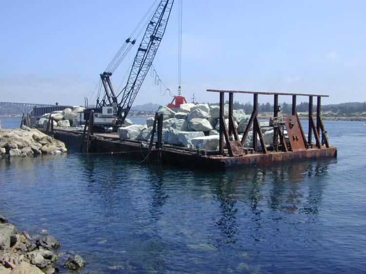
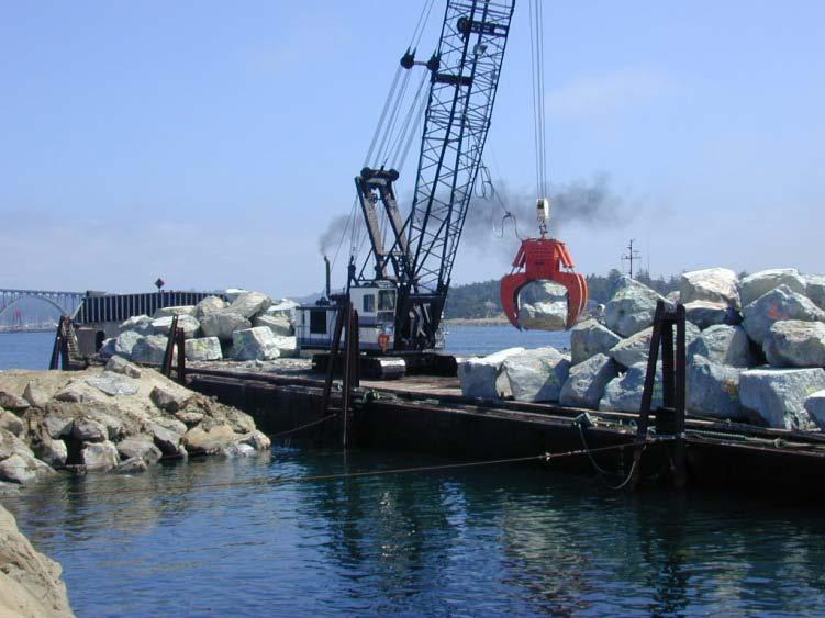
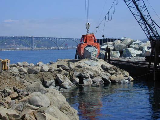
72 Figure 36 (continued) 67

73 The following existing private facilities may serve as potential offloading sites depending on availability for Corps use: Commercial Site in Ilwaco. For the North Jetty, barges would pull up to a dock at Ilwaco where rock would be transferred by crane onto trucks that would proceed by public road to Cape Disappointment State Park. Trucks would then pass through the park grounds to the staging area adjacent to the jetty. For Jetty A, trucks would proceed through the Coast Guard facility to the staging area near the root of the jetty. Commercial Site in Warrenton. Nygaard Logging has a deep-water offloading site that could be used to offload rock. For the North Jetty/Jetty A, rock would be transferred to trucks that would likely use Highway 101 into Astoria, cross the Astoria-Megler Bridge, and head west through Ilwaco to Cape Disappointment State Park. Trucks would then pass through the park grounds to the staging area adjacent to the jetty. For the South Jetty, rock would be transferred to trucks which would then proceed west through Hammond to Fort Stevens State Park and use the existing park road to staging area adjacent to the jetty. This site needs no improvement to accommodate deep-draft vessels. If existing facilities are not available or do not have adequate capacity to provide access, barge offloading facilities could be constructed at each jetty. North Jetty: Between or on the spur groin at/between Station 50 or 70, a barge offloading facility will be constructed. If wave conditions make it feasible, the spur groin designed for this area will first function as an offloading facility prior to conversion and stone removal to reach the spur s design depth. Otherwise, a separate facility will be installed in the reach between these two stations such that wave conditions allow safe offloading. This offloading facility will require 4-8 dolphins of 3 piles each for vessel tie-up, and sheet-pile installation will be required to shore-up and retain rock at the offloading point. Jetty A: An offloading facility will be sited near the location of the proposed spur groin around Station 81, at the upstream portion of the jetty near the head. The proposed spur groin could not be used for dual purposes, because it would have required additional, unnecessary rock in order to connect the offloading facility with the causeway. A 15-ft causeway will also be constructed along the entire length of the jetty on existing relic stone that runs adjacent to and abutting the upstream eastern portion of the jetty. This facility will likely remain a permanent facility, but may deteriorate due to wave and tidal action. This offloading facility will require 4-8 dolphins of 3 piles each for vessel tie-up, and sheet-pile installation will be required to shore-up and retain rock at offloading point. South Jetty: The South Jetty could have up to two associated offloading sites. One will be located at Parking Lot Area D near the northeastern-most corner of the Spit. The second facility will be located along the jetty and will resemble an extra-large turn-out facility. It is likely to be located somewhere on the northern, channel-side of the jetty and west of Station 270 in order to take advantage of deeper bathymetry and subsequently less need for dredging. The facility at Parking Lot Area D may be removed after 5 or more years depending on hydraulic impacts of the structure and spit. The facility along the jetty will likely be partially removed and rebuilt after each repair to avoid the 68

74 potential for wave-focusing on the jetty. Otherwise, it will remain in place until around Each offloading facility will require 4-8 dolphins of 3 piles each for vessel tie-up, and sheet-pile installation will be required to shore-up and retain rock at offloading point. Dredging for Barge Offloading Facilities Transport of rock would most likely be done by ocean-going barges that require deeper draft (20-22 feet) and bottom clearance than river-going barges when fully loaded. Therefore, dredging will be required to develop each of the barge offloading facilities. Under-keel clearance should be no less than 2 feet. The elevation at barge offloading sites should have access to navigable waters and a dredge prism with a finish depth no higher than -25 feet MLLW, with advance maintenance and disturbance zone depths not to extend below -32 feet MLLW. These facilities should also provide for a maneuvering footprint of approximately 400 feet x 400 feet. The depth along the barge unloading sites would be maintained during the active period for which the rock barges will be unloaded. A clamshell dredge would likely be used for all dredging, though there is a small chance that a pipeline dredge could be feasible but is unlikely to be used. The material to be dredged is medium to fine-grained sand, typical of MCR marine sands. Disposal of material would occur in-water at an existing approved disposal site. The volume of material to be dredged is shown in Table 12; these estimates are based on current bed morphology and may change. Also, maintenance dredging to a finish depth of -25 feet MLLW will be needed before offloading during each year of construction. Dredging is likely to occur on a nearly annual basis for the duration of the project construction period, but this will be intermittent per jetty, depending on which one is scheduled for construction in a particular year. Table 12. Estimated Dredging Volumes for Barge Offloading Facilities Location* Estimated Dredging Volume Approximate (cy) Acres Initial Est. Maintenance** North Jetty 30,000 30, Jetty A 60,000 80, South Jetty 20,000 20, South Jetty - Parking Area D 20,000 20, * Some of the locations will not be used on an annual basis; it depends on the construction schedule for each jetty. **All dredging will be based on surveys that indicate depths shallower than -25 feet MLLW. Clamshell dredging is done using a bucket operated from a crane or derrick that is mounted on a barge or operated from shore. Sediment removed from the bucket is generally placed on a barge before disposal. This type of dredge is typically used in shallow water areas. The following overall impact minimization practices and best management practices (BMPs) will be used for all maintenance dredging for offloading facilities. 1. To reduce the potential for entrainment of juvenile salmon or green sturgeon, the cutterheads will remain on the bottom to the greatest extent possible and only be raised 3 feet off the bottom when necessary for dredge operations. 69

75 2. To reduce turbidity, if a clamshell bucket is used, all digging passes shall be completed without any material, once in the bucket, being returned to the wetted area. Not dumping of partial or half-full buckets of material back into the project area will be allowed. No dredging of holes or sumps below minimum depth and subsequent redistribution of sediment by dredging dragging or other means will be allowed. All turbidity monitoring will comply with Sate 401 Water Quality Certification Conditions. 3. If the Captain or crew operating the dredges observes any kind of sheen or other indication of contaminants, he/she will immediately stop dredging and notify the Corps environmental staff to determine appropriate action. 4. If routine or other sediment sampling determines that dredged material is not acceptable for unconfined, in-water placement, then a suitable alternative disposal plan will be developed in cooperation with the NMFS, EPA, Oregon Department of Environmental Quality (ODEQ), Washington Department of Ecology (WDOE), and other agencies. Dredged Material Disposal Sites Two dredged material disposal sites, the Shallow Water Site (SWS) and the North Jetty site, are located near the North Jetty. These are the most likely sites to be used. Modeling has showed that the potential changes to the two disposal sites from the proposed action would not inhibit their use as disposal sites. Spur groin construction at the North Jetty would avoid the North Jetty disposal site. The northern-most cells of this site immediately adjacent to the jetty will be avoided to reduce the possibility of vessel impact with the spur groins. Pile Installation and Removal As mentioned earlier, inclement weather and sea conditions during the preferred in-water work window (IWWW) preclude safe working conditions during this time period. Therefore, installation of piles is most likely to occur outside the IWWW. For initial construction of all four facilities combined, approximately up to 96 Z- or H-piles could be installed as dolphins, and up to 373 sections of Z or H pile to retain rock fill. They will be located within 200-ft of the jetty structure. Because the sediments in the region are soft (sand), use of a vibratory driver to install piles is feasible and will be used when necessary. The presence of relic stone may require locating the piling further from the jetty so that use of this method is not precluded by the existing stone. The dolphins/z- and H-piles would be composed of either untreated timber or steel piles installed to a depth of approximately 15 to 25 feet below grade in order to withstand the needs of off-loading barges and heavy construction equipment. Because vibratory hammers will be implemented in areas with velocities greater than 1.6 ft/s, the need for hydroacoustic attenuation is not an anticipated issue. Piling will be fitted with pointed caps to prevent perching by piscivorous birds to minimize opportunities for avian predation on listed species. Some of the pilings and offloading facilities will be removed at the end of the construction period. Rock Placement Placement of armor stone and jetty rock on the MCR jetties would be accomplished by land or limited water-based equipment. Only clean stone will be used for rock placement, where appropriate and feasible. Where appropriate, there may also be some re-working and reuse of the existing relic and jetty prism stone. Fill for the jetty haul roads will not be cleaned prior to 70

76 installation. Dropping armor stone from a height greater than 2 feet will be prohibited. During placement there is a very small chance of stone slippage down the slope of the jetty. However, this is unlikely to occur due to the size and cost of materials and placement. Another approach to water-based rock placement would be via a jack-up barge. This would only be applicable at the South Jetty. For armor stone and rock placement at the head, a jack-up barge with crane could be used to serve as a stable work platform (Figure 37). Once into place, the jack-up barge would be jacked up on six legs so that the deck is at the same elevation as the jetty. The legs are designed to use high-pressure water spray from the end of the legs to agitate the sand and sink the legs under their own weight. The jacking process does not use any lubricants that contain oils, grease, and/or other hydrocarbons. The stone and rock will be barged to the jackup barge and offloaded onto the jetty head. The jackup barge will keep moving around the head of the jetty to complete the work. A jack-up barge would not be used on the North Jetty or Jetty A to avoid interference with navigation of fishing boats and crab and fish migrations. Figure 37. Illustration of a Jack-up Barge For land-based rock placement, a crane or a large track-hoe excavator could be situated on top of the jetty. The placement operation would require construction of a haul road along the jetty crest within the proposed work area limits. The crane or excavator would use the haul road to move along the top of jetty. Rock would be supplied to the land-based placement operation by land and/or marine-based rock delivery. For marine-based rock, the land-based crane or excavator would pick up rock directly from the barge or from a site on the jetty where rock was previously offloaded and stockpiled, and then place the rock within the work area. For land-based rock, the crane or excavator would supply rock via a truck that transports rock from the stockpile area. The crane or excavator would advance along the top of the jetty via the haul road as the work is completed. 71

77 In order to place stones, a haul road will be constructed on the 30-ft crest width of each jetty to allow crane and construction vehicle access. Roads will consist of an additional 3-ft of top fill material, which could also entail an additional 2-ft of width spill-over. These roads will remain in place for the duration of construction. Due to ocean conditions and the wave environment, these roads will likely need yearly repair and replacement. They will not be removed upon completion. Ramps from the beach up to the jetty road will also be constructed to provide access at each jetty. At approximately 1000-ft intervals, turnouts to allow equipment access and passage will be constructed on the North and South jetties. These will consist of 50-ft long sections that are an additional 20-ft wide. Some of this stone for these facilities may encroach below MLLW. On the North Jetty, there will be approximately 2 turnouts. South Jetty will have approximately 8 turnouts with two additional larger-sized turnouts. These larger turnouts will be in the range of 300-ft long with an additional 20-ft width. One of these larger turnouts will function as an offloading facility on South Jetty. At Jetty A, the causeway will function as the turnout facility. Towards the head of each jetty, additional crane set up pads will be constructed at approximately 40-ft increment to allow crane operation during the placement of the larger capping stones. Setup pads will roughly entail the addition of 8 extra feet on each side of the crest for a length of about 50-ft. Some of this stone for these facilities may encroach below MLLW. Approximately 5 set-up pads will be required to construct each jetty head. Construction Staging, Storage, and Rock Stock Piles Jetty repairs and associated construction elements entail additional footprints for activities involving equipment and supply staging and storage, parking areas, access roads, scales, general yard requirements, and rock stock pile areas. It was determined that for most efficient work flow and placement, a 2-year rock supply would be maintained on site and would be continuously replenished as placement occurred on each jetty. In order to estimate the area needed, a surrogate area was determined for a reference volume of 8,000 cy, which was then used to extrapolate the area needed at each jetty. These results are shown in Table 13. Table 13. Acreages Needed for Construction Staging, Storage, and Rock Stock Piles Location Approximate Acres North Jetty 31 Jetty A 23 South Jetty 44 Several actions will be taken to avoid and minimize impacts from these activities. Staging and stockpiles will remain above MHHW and where feasible have also been sited to avoid impacts to wetlands and habitats identified as having higher ecological value. In order to maintain erosive resilience along the shoreline, a vegetative buffer will be preserved. When available and possible, partial use will be made of existing parking lots. Additional measures specific to each jetty have also been considered. Besides access roads in the areas identified in Figures 33-35, no 72

78 additional roadways or significant roadway improvements are anticipated. Some roadway repair and maintenance will likely be required on existing roads experiencing heavy use by the Corps. At the North Jetty, the lagoon and wetland fill necessary for root stabilization will also serve a dual purpose as for the bulk of staging and storage activities. At the South Jetty, a small spur road will be required to connect the existing road with the proposed staging area and is indicated in Figures The existing road along the neck of the South Jetty that will be used for dune augmentation work may require minor repair/improvements for equipment access. Construction access to the area receiving dune augmentation will be limited to an existing access road along the relic jetty structures at the neck of the spit. Equipment will be precluded from delivery using the access point from Parking Lot B in order to avoid impacts to water quality and razor clam beds in the vicinity of the proposed dune fill area. Grading equipment may have to access the area by driving along the shore, but this route will be used as a last resort and equipment will be limited to dry sand where feasible. Additionally, the proposed actions will avoid the more sensitive habitat areas south of Parking Lot D. If possible, the project will avoid and minimize impacts to the adjacent marshland by allowing crossing between the construction area and jetty via a Bailey bridge, which may require small removable abutments on either end of the marsh crossing. Otherwise a series of culverts and associated fill will be installed, or equipment will be required to enter and exit from the same access road on the northeast end of the main staging area indicated in Figures Additionally, at the outlet of the marsh complex a culvert will be installed under the construction access road, which will allow continuous hydrologic connectivity between affected portions of the marsh and ocean exchange through the jetty. This will also avoid equipment passage through marsh waters. To connect the staging area to the jetty haul road, a temporary gravel access road would be constructed from the staging area nearest the jetty to the jetty crest. The access road would measure approximately 400 ft in length by 25 ft in width, would be above MHHW, would require approximately 4,000 cy of sand, gravel and rip rap, and would require the installation and removal of a temporary culvert near station to maintain tidal exchange into and out of the intertidal wetland and through the jetty. The staging areas and haul roads, except for the jetty haul road, would be removed and restored to pre-construction conditions once repairs to the jetty are completed. Prior to in-water work for installing the construction access road and culverts across the southern portion of the marsh wetland outlet at the South Jetty, the Corps will conduct fish salvage and implement fish exclusion to and from the wetland complex upstream of the proposed culvert. Also, post-installation of the culvert, the Corps will develop and implement fish monitoring as necessary to ensure that no listed fish species are stranded. If listed fish species are found, NMFS will be contacted immediately to determine the appropriate course of action. At Jetty A, adequate area may not be available for the estimated storage and staging needs. Therefore, construction sequencing will accommodate the supply that can be fit into the acreage 73

79 available. Land-based delivery options may be precluded due to road access constraints, though some existing access may prove available and feasible depending on load and truck sizes. The following measures will also be required at each location to further avoid and minimize impacts to species. Before significant alteration of the project area, the project boundaries will be flagged. Sensitive resource areas, including areas below ordinary high water, wetlands and trees to be protected will be flagged. Chain link fencing or something functionally equivalent will likely encircle much of the construction areas. Temporary Erosion Controls Temporary erosion controls will be in place before any significant alteration of the site. If necessary, all disturbed areas will be seeded and / or covered with coir fabric at completion of ground disturbance to provide immediate erosion control. Erosion control materials (and spill response kits) will remain on-site at all times during active construction and disturbance activities (e.g., silt fence, straw bales). If needed these measures will be maintained on the site until permanent ground cover or site landscaping is established and reasonable likelihood of erosion has passed. When permanent ground cover and landscaping is established, temporary erosion prevention and sediment control measures, pollution control measures and turbidity monitoring will be removed from the site, unless otherwise directed. An Erosion Sediment and Pollution Control Plan (ESPCP) or Stormwater Pollution Prevention Plan (SWPPP), as applicable to each State, will outline facilities and Best Management Practices (BMPs) that will be implemented and installed prior to any ground disturbing activities on the project site, including mobilization. These erosion controls will prevent pollution caused by surveying or construction operations and ensure sediment-laden water or hazardous or toxic materials do not leave the project site, enter the Columbia River, or impact aquatic and terrestrial wildlife. The Corps retains a general 1200-CA permit from Oregon Department of Environmental Quality (DEQ), and will also work with EPA to obtain use of the NPDES General Permit for Stormwater Discharge from Construction Activities. At a minimum, these ESCP and SWPPP plans will include the following elements and considerations. Construction discharge water generated on-site (debris, nutrients, sediment and other pollutants) will be treated using the best available technology. Water quality treatments will be designed, installed, and maintained in accordance with manufacturer s recommendation and localized conditions. In addition, the straw wattles, sediment fences, graveled access points, and concrete washouts may be used to control sedimentation and construction discharge water. Construction waste material used or stored on-site will be confined, removed, and disposed of properly. No green concrete, cement grout silt, or sandblasting abrasive will be generated at the site. Emergency Response To avoid the need for emergency response a Corps Government Quality Assurance Representative (GQAR) will be on-site or available by phone at all times throughout construction. Emergency erosion/pollution control equipment and best management practices will be on site at all times; Corps staff will conduct inspections and ensure that a supply of sediment control materials (e.g., silt fence, straw bales), hazardous material containment booms 74

80 and spill containment booms are available and accessible to facilitate the cleanup of hazardous material spills, if necessary. Hazardous Materials A description of any regulated or hazardous products or materials to be used for the project, including procedures for inventory, storage, handling and monitoring, will be kept on-site. Fuels or toxic materials associated with equipment will not be stored or transferred near the water, except in a confined barge. Equipment will be fueled and lubricated only in designated refueling areas at least 150 feet away from the MHHW, except in a confined barge. Spill Containment and Control A description of spill containment and control procedures will be on-site, including: notification to proper authorities, specific cleanup and disposal instructions for different products, quick response containment and cleanup measures that will be available on the site including a supply of sediment control materials, proposed methods for disposal of spilled materials, and employee training for spill containment. Generators, cranes, and any other stationary power equipment operated within 150-feet MHHW will be maintained as necessary to prevent leaks and spills from entering the water. Vehicles / equipment will be inspected daily for fluid leaks and cleaned as needed before leaving staging and storage area for operation within 150 feet of MHHW. Any leaks discovered will be repaired before the vehicle / equipment resumes service. Equipment used below MHHW will be cleaned before leaving the staging area, as often as necessary to remain grease-free. Additionally, the Corps proposes to use a Wiggins fast fuel system or equivalent to reduce leaks during fueling of cranes and other equipment in-place on the jetties (Figure 38). Also, spill pans will be mounted under the crane and monitored daily for leaks. Water Quality Monitoring In-water work will require turbidity monitoring that will be conducted in accordance with 401 Water Quality Certifications Conditions to ensure the project maintains compliance with State water quality standards. Turbidity exceedences are expected to be minimal due to the large size of stone being placed. Dynamic conditions at the jetties in the immediate action area preclude the effective use of floating turbidity curtains (or approved equal). Sedimentation and migration of turbid water into the Columbia is not expected to be a significant issue. Best management practices will be used to minimize turbidity during in-water work. Turbidity monitoring will be conducted and recorded each day during daylight hours when in-water work is conducted. Representative background samples will be taken according to the schedule set by the resource agencies at an undisturbed area up-current from in-water work. Compliance samples will be taken on the same schedule, coincident with timing of background sampling, down-current from in-water work. Compliance sample will be compared to background levels during each monitoring interval. Additional 401 Water Quality Certification conditions and protocols may be required. 75

81 Figure 38. Fast Fuel System 76

82 WETLAND MITIGATION AND HABITAT IMPROVEMENTS The selected plan design and construction methods for repair and rehabilitation of the MCR jetties have been developed and refined to take advantage of opportunities to avoid and minimize the project s ecological impacts to habitats and species. As required under the Clean Water Act, the Corps will mitigate for impacts to wetlands which could not be otherwise avoided or minimized. The Corps has also incorporated habitat improvements into the proposed action to assist with the recovery of ESA-listed salmonid habitats and ecosystem functions and processes. These actions are not proposed to directly mitigate or compensate for any Project-related impacts to ESA-listed salmonids. The habitat improvement components of the overall ecosystem restoration action are proposed as Conservation Measures under Section 7(a) (1) of the ESA and have been included into the proposed action by the Corps. These actions are the Corps affirmative commitment to fulfill responsibility to assist with conservation and recovery of ESAlisted salmonids. Habitat improvement features will be designed to create or improve salmonid habitat, specifically tidal marsh, swamp, and shallow water and flats habitat, and to improve fish access to these habitat features. In addition, one of the features would create habitat for snowy plover. Habitat improvement and wetland mitigation plans currently address three general categories: actions that create, improve, and restore wetlands, actions that improve in-water habitats, and actions that restore upland habitats. From the list of possible wetland mitigation and habitat improvement features shown in Table 14, one or a combination of projects will be selected for further development and implementation. Selection will occur with input from the AMT and work is anticipated to occur concurrent with jetty repair actions. 77

83 Table 14. Possible Wetland Mitigation and Habitat Improvement Features Feature/Site Area Affected Type and Function Trestle Bay Walooskee to Youngs Bay Walooskee to Youngs Bay Slough to Youngs River 5-8 acres with potential of additional acres ~151 acres ~39 acres ~ acres Estuarine Saltwater Marsh Wetland and Intertidal Mudflat Creation and Restoration Create and expand estuarine intertidal brackish saltwater marsh wetland habitat. Expand and restore Lyngby sedge plant community. Expand/increase intertidal shallow water habitat, including dendritic mud flats and off-channel habitat. Remove and control invasive species and improve/restore diversity and density of native plant assemblages. Increase habitat complexity for fisheries benefit. Potentially expand floodplain terrace and improve riparian function. (Re)introduce natural tidal disturbance regime to area currently upland dunes. Levee Breach for Estuarine Emergent Wetland and Brackish Intertidal Shallow-water Habitat Restoration Restore connection between Walooskee and Youngs River via levee breach. Restore and expand estuarine intertidal brackish marsh wetland habitat. Expand and restore Lyngby sedge and native estuarine vegetation community to improve trophic foodweb functions. Restore and expand brackish intertidal shallow water habitat including dendritic mud flats and off-channel edge habitat. Remove and control invasive species and improve/restore diversity and density of native plant assemblages. Increase habitat access and complexity for fisheries benefit including expanded foraging, rearing, and refugia habitat types. Improve riparian function. Potentially restore floodplain terrace and increase flood storage capacity. (Re)introduce natural tidal disturbance regime to area currently diked pasture land. Restore hydrologic regime and restore/improve water quality function. Improve capacity for additional carbon sequestration via native root masses. Increase and restore hyporheic functions for improved water quality and potential creation of cold water refugia. Levee Breach and/or Tide Gate Retrofits for Emergent Wetland and Intertidal Shallow-water Habitat Restoration Restore connection with Walooskee River via levee breach and/or tide gate retrofits. Restore and expand intertidal marsh wetland habitat. Expand and restore native vegetation community to improve trophic foodweb functions. Restore and expand intertidal shallow water habitat including dendritic and off-channel edge habitat. Remove and control invasive species and improve/restore diversity and density of native plant assemblages. Increase habitat access and complexity for fisheries benefit including expanded foraging, rearing, and refugia habitat types. Improve riparian function. Potentially restore floodplain terrace and increase flood storage capacity. Restore hydrologic and natural tidal disturbance regime and restore/improve water quality function to area currently functioning as diked pasture land. Improve capacity for additional carbon sequestration via native root masses. Increase and restore hyporheic functions for improved water quality and potential creation of cold water refugia. Levee Breach for Estuarine Wetland and Intertidal Restoration Restore connection between Slough and Youngs River via levee breach. Restore and expand estuarine intertidal brackish marsh wetland habitat. Expand and restore Lyngby sedge and native estuarine vegetation community to improve trophic foodweb functions. Restore and expand brackish intertidal shallow water habitat including dendritic mud flats and off-channel edge habitat. 78

84 Feature/Site Area Affected Type and Function Remove and control invasive species and improve/restore diversity and density of native plant assemblages. Increase habitat access and complexity for fisheries benefit including expanded foraging, rearing, and refugia habitat types. Improve riparian function. Potentially restore floodplain terrace and increase flood storage capacity. Restore hydrologic and natural tidal disturbance regimes to an area currently functioning as diked pasture land. Improve capacity for additional carbon sequestration via native root masses. Increase and restore hyporheic functions for improved water quality and potential creation of cold water refugia. Youngs River - Diked Farmland, Freshwater Intertidal Restoration Tributary Cr. to Youngs River Tributary Cr. and Slough to the Columbia River - near Clatskanie acres With potential up to 80 acres ~5 or more acres Up to ~43 acres Levee Breach for Wetland and Intertidal Restoration Restore connection with Youngs River via levee breach. Restore and expand freshwater intertidal wetland habitat. Expand and restore native vegetation community to improve trophic foodweb functions. Restore and expand intertidal shallow water habitat including dendritic mud flats and off-channel edge habitat. Remove and control invasive species and improve/restore diversity and density of native plant assemblages. Increase habitat access and complexity for fisheries benefit including expanded foraging, rearing, and refugia habitat types. Improve riparian function. Potentially restore floodplain terrace and increase flood storage capacity. (Re)introduce natural tidal disturbance regime to area currently diked pasture land. Restore hydrologic regime and restore/improve water quality function. Increase and restore hyporheic functions for improved water quality and potential creation of cold water refugia. Estuarine Wetland and Intertidal Restoration; Tributary Reconnection to Youngs Bay Convert diked pasture land to brackish estuarine wetland and shallow water intertidal habitat. Improve and restore hydrologic regime and increase regular hydrologic connectivity between Crosel Cr. And Youngs Bay estuary. Improve and restore fish passage and provide access throughout greater range of flows to off-channel juvenile rearing, refuge and foraging habitats. Remove and control invasive species and improve/restore diversity and density of native plant assemblages. Increase habitat complexity for fisheries benefit. Improve adult salmonid access to headwaters and potential spawning habitat. Potentially expand floodplain terrace and improve riparian function. (Re)introduce natural flow regime and tidal disturbance regime to area currently functioning as pasture land. Levee Breach and/or Tide Gate Retrofits for Emergent Wetland and Intertidal Shallow-water Habitat Restoration and Tributary Reconnection Restore connection between Tandy and Graham creeks and Westport Slough and Columbia River via levee berach and/or tide gate retrofits. Restore and expand intertidal wetland habitat. Expand and restore native vegetation community to improve trophic foodweb functions. Restore and expand intertidal shallow water habitat including dendritic and off-channel edge habitat. Remove and control invasive species and improve/restore diversity and density of native plant assemblages. Increase habitat access and complexity for fisheries benefit including expanded foraging, rearing, and refugia habitat types. Improve riparian function. Potentially restore floodplain terrace and increase flood storage capacity. Restore hydrologic and natural tidal disturbance regime and restore/improve water quality function to area currently functioning as diked pasture hayfields. 79

85 Feature/Site Area Affected Type and Function Improve capacity for additional carbon sequestration via native root masses. Increase and restore hyporheic functions for improved water quality and potential creation of cold water refugia. Improve adult salmonid access to headwaters and potential spawning habitat. Knappa - Warren Slough Snowy Plover Work on Clatsop Spit Wetland Creation at Cape Disappointment Tide Gate Retrofits for Salmonid Passage ~100 or more acres Up to ~22 acres Up to ~10 acres Variable Preservation and Expansion of Estuarine Intertidal Restoration; Improve Tributary Reconnection for Fish Passage Maintain and enhance evolving restoration that has occurred since inundation of previously diked pasture land to estuarine wetland and shallow intertidal habitat. Maintain restored ecosystem function and intertidal shallow water habitat established post-breach. Maintain and enhance restored hydrologic regime and increase regular hydrologic connectivity between Hall Cr. and Warren Slough. Maintain and improve existing fish passage and provide access throughout greater range of flows to off-channel juvenile rearing, refuge and foraging habitat types. Maintain and increase habitat complexity for fisheries benefit. Improve adult salmonid access to headwaters and potential spawning habitat. Remove and control invasive species and improve/restore diversity and density of native plant assemblages; Improve riparian function as appropriate. Potentially expand floodplain terrace. Maintain restored natural tidal disturbance regime, dendritic channels, and connection between Hall Cr. and Warren Slough. Forego Revegetation and Convert Upland Areas to Snowy Plover Habitat Convert upland scrub-shrub habitat with invasive species to snowy plover habitat via periodic tilling and application of shell hash. Creation and Expansion of Interdunal Wetland Complex Excavation of new interdunal wetlands adjacent to existing wetlands. Establishment of native wetland plant communities and removal of invasive species around a buffer zone. Restoration or provision of hydrology to newly excavated wetlands via appropriate elevation design. Restoration of wetland connectivity between existing fragmented wetlands via culvert retrofits, if feasible. Select Tributaries from ODFW Priority Culvert Repair List - Tributary Reconnection Restore and improve existing fish passage and provide access throughout greater range of flows to off-channel juvenile rearing, refuge and foraging habitat types. Restore and increase habitat complexity for fisheries benefit. Restore and improve adult salmonid access to headwaters and potential spawning habitat. 80

86 Wetlands and shallow-water habitat will be filled and converted as a result of the project. Official wetland delineations have not yet been completed for all three of the jetties. However, available preliminary information has allowed the Project Delivery Team (PDT) to site construction activities and features to reduce anticipated impact to wetlands. This information has also been used to calculate initial estimates regarding the possible acreage of impacts. The approximated acreages identified as potentially impacted are North Jetty ~4.78, South Jetty up to ~22 and Jetty A up to ~11. This comes to an estimated total of ~38.28 acres of potential wetlands impacts. To reiterate, official delineations must be completed, and these numbers will be revised accordingly after report results and project design details are further developed and available. These estimates are on the conservatively high end of what final wetland impacts will likely be. In-water habitats, both shallow intertidal and deeper subtidal areas will also be affected by the project. Habitat conversions will occur from maintenance dredging and placement of the spur groins, jetty cross-sections, turnouts, barge offloading facilities, and causeways. There will also be permanent lagoon fill at the North Jetty root. Without drawing a distinction between depths, initial acreage estimates for all in-water impacts include North Jetty ~11.75, South Jetty ~21.2, and Jetty A ~7.23. This comes to an approximated total of ~40.18 acres of potential in-water conversions. Shallow-water habitat is especially important to several species in the estuary; therefore, specific initial estimates were also calculated regarding shallow-water habitat (shallow here defined as -20-ft or -23-ft below MLLW). About 30 acres (out of the ~40 mentioned above) of area at these depths will be affected by groins, maintenance dredging, and construction of the causeways and barge offloading facilities. However, this estimate does NOT including any expansion of the jetty s existing footprint or overwater structures from barge offloading facilities. The approximate acreage breakdowns entail: spur groin fill = 1.56 (shallow defined as -20-ft or less below MLLW; ~3.26 total area including all depths); dredge for barges ~20, likely all shallow (less than -23-ft deep below MLLW); and causeway fill~ 7, likely all shallow (less than -23 ft deep below MLLW). For this analysis, there was no distinction drawn between periodically exposed intertidal habitat and shallow-water sandflat habitat. As with wetland estimates, these approximations will be updated as project designs are refined and as additional analyses and surveys are completed to quantify changes in jetty and dune cross sections. Ultimately the project seeks to achieve no net loss in wetland habitat, to protect, improve and restore overall ecosystem functions, and to provide actions that are anticipated to benefit listed species in the vicinity of the project. Towards that end, specific project footprints and activities described above have been identified, categorized, and quantified with conservative estimates where appropriate. The calculated extents were strictly based on the area of habitat that was converted. They did not include value or functional assignments regarding the significance of the conversion, whether it was a beneficial, neutral, or detrimental effect, nor if conversions created unforeseen, indirect far-field effects. For example, acreage of conversion for shallow sandy sub-tidal habitat to rocky sub-tidal habitat was calculated in the same manner as conversion from shallow intertidal habitat to shallow sub-tidal habitat. Per initial consultation with resource agencies, a preliminary suggested ratio of 2:1 for wetland mitigation will likely be required. This is described in Table 15. These estimated footprints will likely change slightly during final design and after updated wetland delineations are completed. 81

87 Table 15. Maximum Estimated Acreages for Habitat Improvement and Wetland Mitigation Jetty Wetland In-water Upland Replanting North Jetty Total South Jetty Total Jetty A Total TOTAL Wetland and Habitat Improvements Specific opportunities have been identified in the Columbia River estuary and Youngs Bay (see Table 14) and are under consideration to improve and restore functions affected in each of the generalized habitat categories (wetland, in-water, and upland). Depending on further development of wetland mitigation and habitat improvement alternatives, a specific project or combination of projects will be designed and constructed concurrently as the proposed repair and rehabilitation options are completed over time. Mitigation actions and extents will be commensurate with wetland impacts and ratios identified. Proposed projects are subject to further analysis, and unforeseen circumstances may preclude further development of any specific project. In all cases, final selection, design, and completion of specific improvement features is contingent on evolving factors and further analyses including hydraulic and hydrologic conditions, real estate actions, cultural resource issues, etc. For this reason a suite of potential proposals has been identified, and subsequent selection of one or some combination of projects and designs will occur during continued discussion with resource agencies participating on the Adaptive Management Team. These wetland mitigation and habitat improvement measures will therefore require additional Consultations, and it is anticipated that the AMT will facilitate in this process. It is also anticipated that a programmatic Opinion similar to SLOPES or Limit 8 may be useful to fulfill clearance requirements. Actions adjacent to or onsite in the vicinity of the North and South Jetties that could potentially mitigate wetland impacts include: excavation of low and high saltwater marsh wetlands and new interdunal wetlands adjacent to existing wetlands; establishment of native wetland plant communities and removal of invasive species around a buffer zone for wetlands; restoration or provision of hydrology to newly excavated wetlands via appropriate elevation design; and/or restoration of wetland connectivity between existing fragmented wetlands. Offsite opportunities for wetland mitigation in the estuary that warrant further investigation are associated with: levee breaches, inlet improvements, or tide gate retrofits, as appropriate. Purchasing mitigation bank credits may be a possibility, though this is currently constrained by limitations of service area and availability of appropriate wetland types. However, private farmlands behind existing levees may provide wetland mitigation opportunities to pursue further. Hydrology and vegetative communities are heavily influenced by elevation; therefore providing improved hydrology combined with strategic excavation and appropriate plantings should result in a simple and selfsustaining design and outcome. Actions to provide benefits and improvements to in-water habitat include the following opportunities: levee breaches, inlet improvements, or tide gate retrofits, as appropriate. Additional associated actions include: excavation in sand dunes and uplands to specified design elevations in order to create additional intertidal shallow water habitat with dendritic channels 82

88 and mud flats, and excavation for potential expansion of the floodplain terraces. Though conceptually considered, specific opportunities for additional projects such as the following were not identified but could warrant further investigation if none of the projects in the list is determined to be feasible: removal of overwater structures and fill in the estuary; removal of relic pile-dike fields; removal of fill from Trestle Bay or elsewhere; removal of shoreline erosion control structures and replacement with bioengineering features; beneficial use of dredge material to create ecosystem restoration features (Lois Island Embayment is an example from Columbia River Channel Improvement that may be applicable here); and restoration of eelgrass beds. Certain pile fields and engineering features may be providing current habitat benefits that could be lost with removal, and such actions would require appropriate hydraulic analysis coordination with engineers and resource agencies. For potential habitat improvement projects located in Trestle Bay, there is additional monitoring and assessment opportunity. A separate hydraulic/engineering study should investigate whether or not an expansion of low-energy, intertidal habitat near Swash Lake could effectively provide additional storage capacity and affect circulation in the Bay such that erosive pressure at neck of Clatsop Spit could be reduced. The previous 1135 action which breached a section of the relic jetty structure is speculated to have been the cause of increased circulation and erosion. It would be worth evaluating whether or not projects that expand floodplain and intertidal areas in the Bay provide significant energy dissipation and additional low-energy storage capacity to offset or redirect erosive pressures. Alternatively, if other habitat improvement concepts are pursued that include removal of additional piles or creation of additional inlets; it would be worth investigating whether these actions could have indirect positive impacts that further reduce concern with erosion at the neck. Evaluating actions in this light would provide valuable information and insight regarding possible solutions and concerns for erosion and breaching at the neck area of Clatsop Spit on Trestle Bay. Post-construction upland restoration would include the following actions: re-establishing native grasses, shrubs, and trees where appropriate; controlling and removing invasive species like scotch broom and European beach grass in the project vicinity; and re-grading/tilling the area to restore natural contours. Oregon Parks and Recreation Department has requested that the Corps utilize the State Forester as one resource for determining optimal revegetation plans. On the Clatsop Spit there is also a unique opportunity to partner with U.S. Fish and Wildlife and Oregon Parks and Recreation Department (OPRD) regarding creation and management of snowy plover habitat on the Spit. This would be an alternative to re-vegetative restoration of the uplands. The OPRD is currently developing a Habitat Conservation Plan in the area to address snowy plover habitat management prior to an anticipated designation of Critical Habitat by US Fish and Wildlife. There may be locations in the vicinity and away from projected construction and staging areas to convert upland habitat to snowy plover habitat via invasive species removal, tilling, and application of shell hash. Ongoing operation and maintenance during the project via regular tilling and shell hash distribution could possibly be coordinated between the agencies through a vehicle such as a Memorandum of Agreement or similar avenue. Refinement and implementation of this wetland mitigation and habitat improvement plan will help protect species and habitats while restoring wetland functions affected by the MCR project. 83

89 Monitoring and maintenance of wetland mitigation and habitat improvement actions will likely be required to ensure successful establishment of goals and satisfactory return on investment. Regular coordination with the AMT will further facilitate selection and implementation of wetland mitigation and habitat improvement actions that appropriately meet the framework for successful restoration, protection, and preservation of ESA listed species and high-value habitat. ACTION AREA Action area means all areas to be affected directly or indirectly by the federal action and not merely the immediate area involved in the action (50 CFR ). For this consultation, the action area includes (see Figure 1): (1) an area extending 10 miles offshore from Columbia River mile -1; (2) extending 5 miles north and 5 miles south of river mile -1, including all terrestrial habitats; (3) extending upstream as far as the Astoria-Megler Bridge, river mile 13.5; and (4) all areas where quarried stone will be transported, including offshore and inland navigation channels in the Pacific ocean extending as far north as Vancouver B.C. in the Puget Sound, and as far south as Eureka, and Humbolt Bay, California. See Figures for route illustrations. The sixth field HUCs in the vicinity of the MCR include: Baker Bay-Columbia River ; Necanicum River-Frontal Pacific Ocean ; Youngs River- Frontal Columbia River ; Long Beach-Frontal Pacific Ocean and Wallacut River-Frontal Columbia River Federally listed marine and anadromous fish, mammal, and turtle species are present in the action area (Table 16), as well as EFH species including five coastal pelagic species, numerous Pacific Coast groundfish species, and coho and Chinook salmon (Table 17). Vessels transporting rock from Canada or Puget Sound sources will travel through areas where bocaccio (Sebastes paucispinis), canary rockfish (Sebastes pinniger), yelloweye rock fish (Sebastes ruberrimus), and Puget Sound Steelhead (Oncorhynchus mykiss) are generally found. However, barge traffic is not expected to encounter these species and therefore will not affect behavior or habitat of these species. Furthermore, these species are not expected to occur in the vicinity of the MCR jetties where the bulk of the proposed actions will occur. Critical habitat also has not been designated for these species. Therefore, it is anticipated that the proposed action will have no effect on these species, and they will not be included further in this analysis. The same scenario is applicable to Puget Sound Chinook salmon (Oncorhynchus tshawytscha), Hood Canal summer-run Chum salmon (O. keta), and Ozette Lake Sockeye salmon (O. nerka), which do have critical habitat listed in areas where barge traffic may occur. However, the proposed action is also not expected to have any effects on these species or their critical habitat; therefore, these species will also not be included further in this analysis. 84

90 Table 16. Federal Register Notices for Final Rules that List Threatened and Endangered Species, Designate Critical Habitats, or Apply Protective Regulations to Species under Consideration Listing status: T means listed as threatened under the ESA; E means listed as endangered; P means proposed. Species Listing Status Critical Habitat Protective Regulations Marine and Anadromous Fish Chinook salmon (Oncorhynchus tshawytscha) Lower Columbia River T 6/28/05; 70 FR /02/05; 70 FR /28/05; 70 FR Upper Willamette River T 6/28/05; 70 FR /02/05; 70 FR /28/05; 70 FR Upper Columbia River spring-run E 6/28/05; 70 FR /02/05; 70 FR ESA section 9 applies Snake River spring/summer run T 6/28/05; 70 FR /25/99; 64 FR /28/05; 70 FR Snake River fall-run T 6/28/05; 70 FR /28/93; 58 FR /28/05; 70 FR Chum salmon (O. keta) Columbia River T 6/28/05; 70 FR /02/05; 70 FR /28/05; 70 FR Coho salmon (O. kisutch) Lower Columbia River T 6/28/05; 70 FR Not applicable 6/28/05; 70 FR Oregon Coast T 2/11/08; 73 FR /11/08; 73 FR /11/08; 73 FR 7816 S. Oregon/N. California Coasts T 6/28/05; 70 FR /5/99; 64 FR /28/05; 70 FR Sockeye salmon (O. nerka) Snake River E 6/28/05; 70 FR /28/93; 58 FR ESA section 9 applies Steelhead (O. mykiss) Lower Columbia River T 1/05/06; 71 FR 834 9/02/05; 70 FR /28/05; 70 FR Upper Willamette River T 1/05/06; 71 FR 834 9/02/05; 70 FR /28/05; 70 FR Middle Columbia River T 1/05/06; 71 FR 834 9/02/05; 70 FR /28/05; 70 FR Upper Columbia River T 1/05/06; 71 FR 834 9/02/05; 70 FR /018/06; 71 FR 5178 Snake River Basin T 1/05/06; 71 FR 834 9/02/05; 70 FR /28/05; 70 FR Green sturgeon (Acipenser medirosris) Southern T 4/07/06; 71 FR /09/09; 74 FR P 5/21/09; 74 FR Eulachon (Thaleichthys pacificus) T 3/18/10; 75 FR Not applicable Not applicable Marine Mammals Steller sea lion (Eumetopias jubatus) Eastern T 5/5/1997; 63 FR / 27/93; 58 FR /26/90; 55 FR /1/09; 50 CFR Blue whale (Balaenoptera musculus) E 12/02/70; 35 FR Not applicable ESA section 9 applies Fin whale (Balaenoptera physalus) E 12/02/70; 35 FR Not applicable ESA section 9 applies Humpback whale (Megaptera novaeangliae) E 12/02/70; 35 FR Not applicable ESA section 9 applies Killer whale (Orcinus orca) Southern Resident E 11/18/05; 70 FR /26/06; 71 FR ESA section 9 applies Sei whale (Balaenoptera borealis) E 12/02/70; 35 FR Not applicable ESA section 9 applies Sperm whale (Physeter macrocephalus) E 12/02/70; 35 FR Not applicable ESA section 9 applies Marine Turtles Green turtle (Chelonia mydas) Excludes Pacific Coast of Mexico & FL ET 7/28/78; 43 FR /02/98; 63 FR ESA section 9 applies Leatherback turtle (Dermochelys coriacea) E 6/02/70 ; 39 FR /5/10; 75FR319; ESA section 9 applies Loggerhead turtle (Caretta caretta) T 7/28/78; 43 FR Not applicable 7/28/78; 43 FR Olive ridley turtle (Lepidochelys olivacea) ET 7/28/78; 43 FR Not applicable ESA section 9 applies 85

91 Table 17. EFH Species and Potential Life Stages in the Action Area EFH Species Egg Larvae Coho salmon (Oncorhynchus kisutch) Chinook salmon (Oncorhynchus tshawytscha) Northern anchovy (Engraulis mordax) Pacific sardine (Sardinops sagax) Pacific mackerel (Scomber japonicus) Jack mackerel (Trachurus symmetricus) Market squid (Loligo opalescens) California Skate (Raja inornata) Soupfin Shark (Galeorhinus galeus) Spiny Dogfish (Squalus acanthias) Ratfish (Hydrolagus colliei) Lingcod (Ophiodon elongates) Cabezon (Scorpaenichthys marmoratus) Kelp Greenling (Hexagrammos decagrammus) Pacific Cod (Gadus macrocephalus) Pacific Hake (Merluccius productus) Sablefish (Anoplopoma fimbria) Butter Sole (Isopsetta isolepis) Curlfin Sole (Pleuronichthys decurrens) English Sole (Parophyrs vetulus) Flathead Sole (Hippoglossoides elassodon) Pacific Sanddab (Citharichthys sordidus) Petrale Sole (Eopsetta jordani) Rex Sole (Glyptocephalus zachirus) Rock Sole (Lepidopsetta bilineata) Salmon Species Young Juvenile Coastal Pelagic Species Juvenile Adult Spawning X X X X X X X X X X X X X X X X X X X X X X X X X X X X X X X X X X X X X X X X X X X X X X X X X X X X X X X X X X X X X X X X X X X X X X X X X X X X X X X X X X X X X 86

92 EFH Species Egg Larvae Sand Sole (Psettichthys melanostictus) Starry Flounder (Platichthys stellatus) Black Rockfish (Sebastes melanops) Brown Rockfish (Sebastes auriculatus) China Rockfish (Sebastes nebulosus) Copper Rockfish (Sebastes caurinus) Quillback Rockfish (Sebastes maliger) Vermilion Rockfish (Sebastes miniatus) Young Juvenile Juvenile Adult Spawning X X X X X X X X X X X X X X X X X X X X X X X X X X X X 87

93 ENDANGERED SPECIES ACT ENVIRONMENTAL ASSESSMENT INTRODUCTION The summaries that follow describe the status of the ESA-listed species, and their designated critical habitats, that occur within the geographic area of this proposed action and are considered in this Assessment. More detailed information on the status and trends of these listed resources, and their biology and ecology can be found in the listing regulations and critical habitat designations published in the Federal Register (see Table 16) and in many publications available from the NMFS Northwest Region, Protected Resources Division in Portland, Oregon. It is likely that climate change will play an increasingly important role in determining the abundance of ESA-listed species, and the conservation value of designated critical habitats, in the Pacific Northwest. During the last century, average regional air temperatures increased by 1.5 F, and increased up to 4 F in some areas (USGCRP 2009). Warming is likely to continue during the next century as average temperatures increase another 3 to 10 F (USGCRP 2009). Overall, about one-third of the current cold-water fish habitat in the Pacific Northwest is likely to exceed key water temperature thresholds by the end of this century (USGCRP 2009). Precipitation trends during the next century are less certain than for temperature but more precipitation is likely to occur during October through March and less during summer, and more of the winter precipitation is likely to fall as rain rather than snow (ISAB 2007, USGCRP 2009). Where snow occurs, a warmer climate will cause earlier runoff so stream flows in late spring, summer, and fall will be lower and water temperatures warmer (ISAB 2007, USGCRP 2009). Higher winter stream flows increase the risk that winter floods in sensitive watersheds will damage spawning redds and wash away incubating eggs (USGCRP 2009). Earlier peak stream flows will also flush some young salmon and steelhead from rivers to estuaries before they are physically mature, increasing stress and the risk of predation (USGCRP 2009). Lower stream flows and warmer water temperatures during summer will degrade summer rearing conditions, in part by increasing the prevalence and virulence of fish diseases and parasites (USGCRP 2009). Other adverse effects are likely to include altered migration patterns, accelerated embryo development, premature emergence of fry, and increased competition and predation risk from warm-water, non-native species (ISAB 2007). The earth s oceans are also warming, with considerable inter-annual and inter-decadal variability superimposed on the longer-term trend (Bindoff et al. 2007). Historically, warm periods in the coastal Pacific Ocean have coincided with relatively low abundances of salmon and steelhead, while cooler ocean periods have coincided with relatively high abundances (Scheuerell and Williams 2005, Zabel et al. 2006, USGCRP 2009). Ocean conditions adverse to salmon and steelhead may be more likely under a warming climate (Zabel et al. 2006). 88

94 STATUS OF THE SPECIES AND CRITICAL HABITAT Salmon and Steelhead Species Description and Limiting Factors The summaries that follow describe the status of ESA-listed salmon and steelhead, and their designated critical habitats that occur within the geographic area of the Proposed Action. Over the past few decades, the sizes and distributions of the populations considered generally have declined due to natural phenomena and human activity, including the operation of hydropower systems, over-harvest, hatcheries, and habitat degradation. Enlarged populations of terns, seals, sea lions, and other aquatic predators in the Pacific Northwest have been identified as factors that may be limiting the productivity of some Pacific salmon and steelhead populations (Bottom et al. 2005, Fresh et al. 2005). The status of species and critical habitat sections are organized by recovery domains to better integrate recovery planning information that NMFS is developing on the conservation status of the species and critical habitats considered in this consultation. Recovery domains are the geographically-based areas that NMFS is using to prepare multi-species recovery plans. Southern green sturgeon are under the jurisdiction of the NMFS Southwest Region, which has not yet convened a recovery team for this species. The four recovery domains relevant to this consultation and the ESA-listed salmon and steelhead species that reproduce in each recovery domain are shown in Table 18. For this consultation, populations that reproduce in Oregon are also identified as one indication of the importance of the action area to the recovery of these species. However, all populations spawning within the Columbia River Basin use the Columbia River mainstem and estuary to complete part of their life history. Table 18. NMFS Recovery Planning Domains and ESA-listed Salmon and Steelhead Species Recovery Domain Willamette-Lower Columbia (WLC) Interior Columbia (IC) Oregon Coast (OC) Southern Oregon Northern California Coasts Species LCR Chinook salmon UWR Chinook salmon CR chum salmon LCR coho salmon LCR steelhead UWR steelhead UCR spring-run Chinook salmon SR spring/summer Chinook salmon SR fall-run Chinook salmon SR sockeye salmon UCR steelhead MCR steelhead SRB steelhead OC coho salmon SONCC coho salmon 89

95 For each recovery domain, a technical review team (TRT) appointed by NMFS has developed, or is developing, criteria necessary to identify independent salmon populations within each species, recommend viability criteria for that species, and analyze factors that limit species survival. The definition of a population used by each TRT is set forth in the viable salmonid population (VSP) document prepared by NMFS for use in conservation assessments of Pacific salmon and steelhead (McElhany et al. 2000). The boundaries of each population are defined using a combination of genetic information, geography, life-history traits, morphological traits, and population dynamics that indicate the extent of reproductive isolation among spawning groups. Understanding population size and spatial extent is critical for the viability analyses, and a necessary step in recovery planning and conservation assessments for any species. If a species consists of multiple populations, the overall viability of that species is a function of the VSP attributes of its constituent populations. Until a viability analysis of a species is completed, the VSP guidelines recommend that all populations should be managed to retain the potential to achieve viable status to ensure a rapid start along the road to recovery, and that no significant parts of the species are lost before the full recovery plan is implemented (McElhany et al. 2000). The status of critical habitat was based primarily on a watershed-level analysis of conservation value that focused on the presence of listed ESA-listed salmon and steelhead and the biological and physical features (i.e., the PCEs) that are essential to their conservation. This analysis for the 2005 designations was completed by Critical Habitat Analytical Review Teams (CHARTs) that focused on large geographical areas corresponding approximately to recovery domains (NOAA Fisheries 2005). Each watershed was ranked using a conservation value attributed to the quantity of stream habitat with PCEs, the present condition of those PCEs, the likelihood of achieving PCE potential (either naturally or through active restoration), support for rare or important genetic or life history characteristics, support for abundant populations, and support for spawning and rearing populations. In some cases, our understanding of these interim conservation values has been further refined by the work of TRTs and other recovery planning efforts that have better explained the habitat attributes, ecological interactions, and population characteristics important to each species. Natural variations in freshwater and marine environments have substantial effects on the abundance of Pacific salmon and steelhead populations. Of the various natural phenomena that affect most populations of salmon and steelhead, changes in ocean productivity are generally considered the most important. Pacific salmon and steelhead are exposed to high rates of natural predation, particularly during freshwater rearing and migration stages. Ocean predation probably contributes to significant natural mortality, although the levels of predation are largely unknown. In general, Pacific salmon and steelhead are eaten by pelagic fishes, birds, and marine mammals. Over the past few decades, the size and distribution of the salmon and steelhead populations considered here, like the other salmon and steelhead that NMFS has listed, generally have declined because of natural phenomena and human activity, including the operation of hydropower systems, over-harvest, hatcheries, and habitat degradation. Enlarged populations of terns, seals, and sea lions in the Pacific Northwest have reduced the survival of some Pacific salmon and steelhead populations. As noted more fully in the status of the critical habitats section below, climate change is likely to play an increasingly important role in determining the 90

96 abundance of salmon and steelhead by exacerbating long-term problems related to temperature, stream flow, habitat access, predation, and marine productivity (CIG 2004, Scheuerell and Williams 2005, Zabel et al. 2006, ISAB 2007). Willamette and Lower Columbia (WLC) Recovery Domain. Species in the WLC Recovery Domain include LCR Chinook salmon, UWR Chinook salmon, CR chum salmon, LCR coho salmon, LCR steelhead, and UWR steelhead. The WLC-TRT identified 107 demographicallyindependent populations of those species (Table 19), including 47 populations that spawn within Oregon. These populations were further aggregated into strata, groupings above the population level that are connected by some degree of migration, based on ecological subregions. All 107 populations use parts of the mainstem of the Columbia River and the Columbia River estuary that flow through Oregon for migration, rearing, and smoltification. The WLC-TRT recommended viability criteria that follow the VSP framework and described biological or physical performance conditions that, when met, indicate a population or species has a 5% or less risk of extinction over a 100-year period (McElhany et al. 2006, see also, NRC 1995). McElhany et al. (2007) applied those criteria to populations in Oregon and found that the combined extinction risk is very high for LCR Chinook salmon, UWR Chinook salmon, CR chum salmon, LCR coho salmon, and moderate for LCR steelhead and UWR steelhead, although the status of those species with populations in Washington is still under assessment. Table 19. Demographically Independent Salmonid Populations in the WLC Recovery Domain and Spawning Populations Species Populations in Spawning Populations WLC in Oregon LCR Chinook salmon UWR Chinook salmon 7 7 CR chum salmon 17 8 LCR coho salmon 24 9 LCR steelhead 23 6 UWR steelhead 5 5 LCR Chinook salmon. This species includes all naturally-spawned populations of Chinook salmon in the Columbia River and its tributaries from its mouth at the Pacific Ocean upstream to a transitional point between Washington and Oregon east of the Hood River and the White Salmon River; the Willamette River to Willamette Falls, Oregon, exclusive of spring-run Chinook salmon in the Clackamas River; and progeny of seventeen artificial propagation programs. The WLC-TRT identified 32 historical populations of LCR Chinook salmon seven in the coastal subregion, six in the Columbia Gorge, and nine in the western Cascades. Twelve of those populations occur within the action area (Table 20) and only Sandy River late fall Chinook is considered viable (McElhany et al. 2007). The major factors limiting recovery of LCR Chinook salmon include altered channel morphology, loss of habitat diversity, excessive sediment, high water temperature, reduced access to spawning/rearing habitat, and harvest impacts (NMFS 2006). 91

97 Table 20. LCR Chinook Salmon Populations Spawning in Oregon Overall viability risk within 100 years: extinct or very high means greater than 60% chance of extinction; relatively high means 60% to 25% risk of extinction; moderate means 25% to 5% risk of extinction, low or negligible means 5% to 1% risk of extinction, very low means less than 1% chance of extinction, and NA means not available. A low or negligible risk of extinction is considered viable. Ecological Subregion Coast Range Columbia Gorge West Cascade Range Stratum Run Timing Spawning Population In Oregon (Watershed) Young Bay Big Creek Clatskanie Scappoose Overall Viability Risk Very High Fall Very High Relatively High Very High Spring Hood Very High Early fall ( tule ) Upper Gorge Very High Fall Hood Very High Lower Gorge Very High Spring Sandy Moderate Early fall ( tule ) Clackamas Very High Sandy Very High Late fall ( bright ) Sandy Low UWR Chinook salmon. The species includes all naturally-spawned populations of spring-run Chinook salmon in the Clackamas River and in the Willamette River, and its tributaries, above Willamette Falls, Oregon, and progeny of seven artificial propagation programs. All seven historical populations of UWR Chinook salmon identified by the WLC- TRT occur within the action area and are contained within a single ecological subregion, the western Cascade Range (Table 21); only the Clackamas population is characterized as viable (McElhany et al. 2007). The major factors limiting recovery of UWR Chinook salmon identified by NMFS include lost/degraded floodplain connectivity and lowland stream habitat, degraded water quality, high water temperature, reduced streamflow, and reduced access to spawning/rearing habitat (NMFS 2006). 92

98 Table 21. UWR Chinook Salmon Populations Overall viability risk within 100 years: extinct or very high means greater than 60% chance of extinction; relatively high means 60% to 25% risk of extinction; moderate means 25% to 5% risk of extinction, low or negligible means 5% to 1% risk of extinction, very low means less than 1% chance of extinction, and NA means not available. A low or negligible risk of extinction is considered viable. Stratum Ecological Subregion West Cascade Range Run Timing Spring Spawning Population In Oregon (Watershed) Clackamas Molalla North Santiam South Santiam Calapooia McKenzie Middle Fork Willamette Overall Viability Risk Low Relatively High Very high Very high Very high Moderate Very high CR Chum salmon. This species includes all naturally-spawned populations of chum salmon in the Columbia River and its tributaries in Washington and Oregon, and progeny of three artificial propagation programs. The WLC-TRT identified 17 historical populations of CR chum salmon and aggregated these into four strata (Myers et al. 2006). Unlike other species in the WLC Recovery Domain, CR chum salmon spawning aggregations were identified in the mainstem Columbia River. These aggregations generally were included in the population associated with the nearest river basin. Three strata and eight historical populations of CR chum salmon occur within the action area (Table 22); of these, none are viable (McElhany et al. 2007). The major factors limiting recovery of CR chum salmon include altered channel morphology, loss of habitat diversity, excessive sediment, reduced streamflow, harassment of spawners and harvest impacts (NMFS 2006). Table 22. CR Chum Salmon Populations Spawning in Oregon Overall viability risk within 100 years: extinct or very high means greater than 60% chance of extinction; relatively high means 60% to 25% risk of extinction; moderate means 25% to 5% risk of extinction, low or negligible means 5% to 1% risk of extinction, very low means less than 1% chance of extinction, and NA means not available. A low or negligible risk of extinction is considered viable. Ecological Subregion Stratum Run Timing Spawning Population In Oregon (Watershed) Young s Bay Overall Viability Risk Very high Coast Range Columbia Gorge West Cascade Range Fall Fall Fall Big Creek Clatskanie Scappoose Lower Gorge Upper Gorge Clackamas Sandy Very high Very high Very high Very high Very high Very high Very high 93

99 LCR coho salmon. This species includes all naturally-spawned populations of coho salmon in the Columbia River and its tributaries in Washington and Oregon, from the mouth of the Columbia up to and including the Big White Salmon and Hood rivers, in the Willamette River to Willamette Falls, Oregon, and progeny of 25 artificial propagation programs. The WLC-TRT identified 24 historical populations of LCR coho salmon and divided these into two strata based on major run timing: early and late (Myers et al. 2006). Three strata and nine historical populations of LCR coho salmon occur within the action area (Table 23). Of these nine populations, Clackamas River is the only population characterized as viable (McElhany et al. 2007). The major factors limiting recovery of LCR coho salmon include degraded floodplain connectivity and channel structure and complexity, loss of riparian areas and large wood recruitment, degraded stream substrate, loss of stream flow, reduced water quality, and impaired passage (NMFS 2007). In general, late coho salmon spawn in smaller rivers or the lower reaches of larger rivers from mid-november to January, coincident with the onset of rain-induced freshets in the fall or early winter. Spawning typically takes place within a few days to a few weeks of freshwater entry. Late-run fish also tend to undertake oceanic migrations to the north of the Columbia River, extending as far as northern British Columbia and southeast Alaska. As a result, late coho salmon are known as Type N coho. Alternatively, early coho salmon spawn in the upper reaches of larger rivers in the Lower Columbia River and in most rivers inland of the Cascade Crest. During their oceanic migration, early coho salmon tend to migrate to the south of the Columbia River and are known as Type S coho salmon. They may migrate as far south as the waters off northern California. While the ecological significance of run timing in coho salmon is fairly well understood, it is not clear how important ocean migratory pattern is to overall diversity and the relative historical abundance of Type N and Type S life histories largely is unknown. Table 23. LCR Coho Salmon Populations Spawning in Oregon Overall viability risk within 100 years: extinct or very high means greater than 60% chance of extinction; relatively high means 60% to 25% risk of extinction; moderate means 25% to 5% risk of extinction, low or negligible means 5% to 1% risk of extinction, very low means less than 1% chance of extinction, and NA means not available. A low or negligible risk of extinction is considered viable. Stratum Ecological Subregion Coast Range Columbia Gorge West Cascade Range N Run Type N and S S Spawning Population In Oregon (Watershed) Young s Bay Big Creek Clatskanie River Scappoose River Lower Gorge Upper Gorge Hood River Clackamas River Sandy River Overall Viability Risk Very High Very High Relatively High Relatively High Very High NA Very high Low Relatively High 94

100 LCR steelhead. The species includes all naturally-spawned steelhead populations below natural and artificial impassable barriers in streams and tributaries to the Columbia River between and including the Cowlitz and Wind rivers, Washington; in the Willamette and Hood rivers, Oregon; and progeny of ten artificial propagation programs; but excluding all steelhead from the Upper Willamette River basin above Willamette Falls, Oregon, and from the Little and Big White Salmon rivers, Washington. The WLC-TRT identified 23 historical populations of LCR steelhead (Myers et al. 2006). Within these populations, the winter-run timing is more common in the west Cascade subregion, while farther east summer steelhead are found almost exclusively. Summer steelhead return to freshwater long before spawning. Winter steelhead, in contrast, return from the ocean much closer to maturity and spawn within a few weeks. Summer steelhead spawning areas in the Lower Columbia River are found above waterfalls and other features that create seasonal barriers to migration. Where no temporal barriers exist, the winterrun life history dominates. Three strata and six historical populations of LCR steelhead occur within the action area (Table 24). Of the populations in Oregon, only Clackamas is viable (McElhany et al. 2007). The major factors limiting recovery of LCR steelhead include altered channel morphology, lost/degraded floodplain connectivity and lowland stream habitat, excessive sediment, high water temperature, reduced streamflow, and reduced access to spawning/rearing habitat (NMFS 2006). Table 24. LCR Steelhead Populations Spawning in Oregon Overall viability risk within 100 years: extinct or very high means greater than 60% chance of extinction; relatively high means 60% to 25% risk of extinction; moderate means 25% to 5% risk of extinction, low or negligible means 5% to 1% risk of extinction, very low means less than 1% chance of extinction, and NA means not available. A low or negligible risk of extinction is considered viable. Ecological Subregion Columbia Gorge Stratum West Cascade Range Run Timing Population Spawning In Oregon (Watershed) Overall Viability Risk Summer Hood River Very High Lower Gorge Relatively High Winter Upper Gorge Moderate Hood River Moderate Winter Clackamas Low Sandy Relatively High UWR steelhead. This species includes all naturally-spawned steelhead populations below natural and artificial impassable barriers in the Willamette River, Oregon, and its tributaries upstream from Willamette Falls to the Calapooia River. The WLC-TRT identified four historical populations of UWR steelhead, all with winter run timing and all within Oregon (Myers et al. 2006). Only winter steelhead historically existed in this area, because flow conditions over Willamette Falls allowed only late winter steelhead to ascend the falls, until a fish ladder was constructed in the early 1900s and summer steelhead were introduced. Summer steelhead have become established in the McKenzie River where historically no steelhead existed, although these fish were not considered in the identification of historical populations. 95

101 UWR steelhead currently are found in many tributaries that drain the west side of the Upper Willamette River basin. Analysis of historical observations, hatchery records, and genetic analysis strongly suggested that many of these spawning aggregations are the result of recent introductions and do not represent a historical population. Nevertheless, the WLC-TRT recognized that these tributaries may provide juvenile rearing habitat or may be temporarily (for one or more generations) colonized during periods of high abundance. One stratum and five historical populations of UWR steelhead occur within the action area (Table 25), although the west-side tributaries population was included only because it is important to the species as a whole, and not because it is independent. Of these five populations, none are viable (McElhany et al. 2007). The major factors limiting recovery of UWR steelhead include lost/degraded floodplain connectivity and lowland stream habitat, degraded water quality, high water temperature, reduced streamflow, and reduced access to spawning/rearing habitat (NMFS 2006). Table 25. UWR Steelhead Populations Overall viability risk within 100 years: extinct or very high means greater than 60% chance of extinction; relatively high means 60% to 25% risk of extinction; moderate means 25% to 5% risk of extinction, low or negligible means 5% to 1% risk of extinction, very low means less than 1% chance of extinction, and NA means not available. A low or negligible risk of extinction is considered viable. Ecological Subregion Stratum West Cascade Range Run Type Winter Population Spawning In Oregon (Watershed) Molalla North Santiam South Santiam Calapooia West-side Tributaries Overall Viability Risk Moderate Moderate Moderate Moderate Moderate Interior Columbia (IC) Recovery Domain. Species in the IC Recovery Domain include UCR spring-run Chinook salmon, SR spring/summer run Chinook salmon, SR fall-run Chinook salmon, SR sockeye salmon, UCR steelhead, MCR steelhead, and SRB steelhead. The IC-TRT identified 82 demographically-independent populations of those species based on genetic, geographic (hydrographic), and habitat characteristics (Table 26). In some cases, the IC-TRT further aggregated populations into major groupings based on dispersal distance and rate, and drainage structure, primarily the location and distribution of large tributaries (IC-TRT 2003). Of the 82 populations identified, 24 have all or part of their spawning range in Oregon, and all 82 use the lower mainstem of the Snake River, the mainstem of the Columbia River, and the Columbia River estuary, or part thereof, in Oregon for migration, rearing, and smoltification. 96

102 Table 26. Demographically Independent Salmonid Populations in the IC Recovery Domain and Spawning Populations Species Populations in IC Spawning Populations in Oregon UCR spring-run Chinook salmon 3 0 SR spring/summer Chinook salmon 31 7 SR fall-run Chinook salmon 1 1 SR sockeye salmon 1 0 UCR steelhead 4 0 MCR steelhead SRB steelhead 25 6 The IC-TRT also recommended viability criteria that follow the VSP framework (McElhany et al. 2006) and described biological or physical performance conditions that, when met, indicate a population or species has a 5% or less risk of extinction over a 100-year period (IC-TRT 2007, see also, NRC 1995). As of this writing, the IC-TRT has applied the viability criteria to 68 populations although it has only completed a draft assessment for 55 populations (see IC-TRT - Current Status Assessments, as of April 21, 2006, available from NMFS Northwest Region, Protected Resources Division in Portland, Oregon). Of those assessments, the only population that the TRT found to be viable was the North Fork John Day population of MCR steelhead. The strength of this population is due to a combination of high abundance and productivity, and good spatial structure and diversity, although the genetic effects of the large number of out-ofspecies strays and of natural spawners that are hatchery strays are still significant long-term concerns. UCR spring-run Chinook salmon. This species includes all naturally-spawned populations of Chinook salmon in all river reaches accessible to Chinook salmon in Columbia River tributaries upstream of the Rock Island Dam and downstream of Chief Joseph Dam in Washington (excluding the Okanogan River), the Columbia River from a straight line connecting the west end of the Clatsop jetty (South Jetty, Oregon side) and the west end of the Peacock jetty (North Jetty, Washington side) upstream to Chief Joseph Dam in Washington, as well as progeny of six artificial propagation programs. The IC-TRT identified four independent populations of UCR spring-run Chinook salmon in the upriver tributaries of Wenatchee, Entiat, Methow, and Okanogan (extirpated), but no major groups due to the relatively small geographic area affected (IC-TRT 2003, McClure et al. 2005). Although none of these populations spawn in Oregon, they all use the Columbia River mainstem and estuary so all adult and juvenile individuals of this species must pass through part of the action area. The IC-TRT considered that this species, as a whole, is at high risk of extinction because all extant populations are at high risk (IC-TRT - Current Status Assessments, as of April 21, 2006, available from NMFS Northwest Region, Protected Resources Division in Portland, Oregon). The major factors limiting recovery of UWR spring-run Chinook salmon include altered channel morphology and floodplain, riparian degradation and loss of in-river large wood, reduced streamflow, impaired passage, hydropower system mortality, and harvest impacts (NMFS 2006). SR spring/summer run Chinook salmon. This species includes all naturally-spawned populations of spring/summer run Chinook salmon in the mainstem Snake River and the Tucannon River, Grande Ronde River, Imnaha River, and Salmon River subbasins; and progeny 97

103 of fifteen artificial propagation programs. The IC-TRT identified 31 historical populations of SR spring/summer run Chinook salmon, and aggregated these into major population groups (IC-TRT 2003, McClure et al. 2005). This species includes those fish that spawn in the Snake River drainage and its major tributaries, including the Grande Ronde River and the Salmon River, and that complete their adult, upstream migration past Bonneville Dam between March and July. Of the 31 historical populations of SR spring/summer run Chinook salmon identified by the IC- TRT, seven occur entirely or partly within Oregon (Table 27). Each of these populations is part of the Grande Ronde and Imnaha River major group, and all face a high risk of extinction (IC- TRT - Current Status Assessments, as of April 21, 2006, available from NMFS Northwest Region, Protected Resources Division in Portland, Oregon). The major factors limiting recovery of SR spring/summer run Chinook salmon include altered channel morphology and floodplain, excessive sediment, degraded water quality, reduced streamflow, and hydropower system mortality (NMFS 2006). Table 27. SR Spring/Summer Run Chinook Salmon Populations in Oregon Overall viability risk within 100 years: high means greater than 25% risk of extinction; moderate means 5% to 25% risk of extinction, low means 1% to 5% risk of extinction; and very low means less than 1% chance of extinction. Major Group Grande Ronde and Imnaha Rivers Spawning Populations in Oregon (Watershed) Abundance Productivity Risk Viability Assessment Spatial Diversity Risk Overall Viability Risk Wenaha River High Moderate High Wallowa-Lostine River High Moderate High Minam River High Moderate High Catherine Creek High Moderate High Upper Grande Ronde High High High Imnaha River mainstem High Moderate High Big Sheep Creek High Moderate High SR fall-run Chinook salmon. This species includes all naturally-spawned populations of fall-run Chinook salmon in the mainstem Snake River below Hells Canyon Dam, and in the Tucannon River, Grande Ronde River, Imnaha River, Salmon River, and Clearwater River, and progeny of four artificial propagation programs. The IC-TRT identified three populations of this species, although only the lower mainstem population exists at present, and it spawns in the lower main stem of the Clearwater, Imnaha, Grande Ronde, Salmon and Tucannon rivers (IC- TRT 2003, McClure et al. 2005). Unlike the other listed Chinook species in this recovery domain, most SR fall-run Chinook have a subyearling, ocean-type life history in which juveniles outmigrate the next summer, rather than rearing in freshwater for 13 to 14 months before outmigration. Adults return to the Snake River basin in September and October and spawn shortly thereafter. The lower mainstem population spawns in the Columbia River mainstem, in part adjacent to Oregon. All adult and juvenile individuals of this species must pass through part of the action area. The IC-TRT has not completed a viability assessment of this species. The 98

104 major factors limiting recovery of SR fall-run Chinook include reduced spawning/rearing habitat, degraded water quality, hydropower system mortality, and harvest impacts (NMFS 2006). SR sockeye salmon. This species includes all anadromous and residual sockeye salmon from the Snake River basin, Idaho, and artificially-propagated sockeye salmon from the Redfish Lake captive propagation program. The IC-TRT identified historical sockeye production in at least five Stanley Basin lakes and in lake systems associated with Snake River tributaries currently cut off to anadromous access (e.g., Wallowa and Payette lakes), although current returns of SR sockeye are extremely low and limited to Redfish Lake (IC-TRT 2007). SR sockeye salmon do not spawn in Oregon, but all adult and juvenile individuals of this species must pass through part of the action area. The major factors limiting recovery of SR sockeye salmon include altered channel morphology and floodplain, reduced streamflow, impaired passage, and hydropower system mortality (NMFS 2006). MCR steelhead. This species includes all naturally-spawned steelhead populations below natural and artificial impassable barriers in streams from above the Wind River, Washington, and the Hood River, Oregon (exclusive), upstream to, and including, the Yakima River, Washington, excluding steelhead from the Snake River basin; and progeny of seven artificial propagation programs. The IC-TRT identified 20 historical populations of MCR steelhead in major groups (IC-TRT 2003, McClure et al. 2005). Ten populations of MCR steelhead occur in Oregon, divided among three major groups (Table 28). Of the 20 historical populations of MCR steelhead identified by the IC-TRT, only the North Fork John Day population currently meets viability criteria, and none of the major groups or the species are considered viable (IC-TRT - Current Status Assessments, as of April 21, 2006, available from NMFS Northwest Region, Protected Resources Division in Portland, Oregon). The major factors limiting recovery of MCR steelhead include altered channel morphology and floodplain, excessive sediment, degraded water quality, reduced streamflow, impaired passage, and hydropower system mortality (NMFS 2006). Table 28. MCR Steelhead Populations in Oregon The Walla Walla population also occurs partly in Washington. Major Group Cascade East Slope Tributaries John Day River Walla Walla and Umatilla Rivers Population (Watershed) Fifteenmile Creek Deschutes Eastside Tributaries Deschutes Westside Tributaries Lower Mainstem John Day River North Fork John Day River Middle Fork John Day River South Fork John Day River Upper Mainstem John Day River Umatilla River Walla Walla River UCR steelhead. This species includes all naturally-spawned steelhead populations below natural and artificial impassable barriers in streams in the Columbia River Basin upstream from the Yakima River, Washington, to the U.S./Canada border, and progeny of six artificial 99

105 propagation programs. Four independent populations of UCR steelhead were identified by the IC-TRT in the same upriver tributaries as for the previous species (i.e., Wenatchee, Entiat, Methow, and Okanogan) and, similarly, no major population groupings were identified due to the relatively small geographic area involved (IC-TRT 2003, McClure et al. 2005). None of these populations spawn in Oregon, although all adult and juvenile individuals of this species must pass through part of the action area. The IC-TRT has not completed a viability assessment of this species, although all extant populations are considered to be at high risk of extinction (IC- TRT - Current Status Assessments, as of April 21, 2006, available from NMFS Northwest Region, Protected Resources Division in Portland, Oregon). The major factors limiting recovery of UCR steelhead include altered channel morphology and floodplain, riparian degradation and loss of in-river large wood, excessive sediment, degraded water quality, reduced streamflow, hydropower system mortality, harvest impacts, and hatchery impacts (NMFS 2006). SRB steelhead. This species includes all naturally-spawned steelhead populations below natural and artificial impassable barriers in streams in the Snake River basin of southeast Washington, northeast Oregon and Idaho, and progeny of six artificial propagation programs. These fish are genetically differentiated from other interior Columbia steelhead populations and spawn at higher altitudes (up to 6,500 feet) after longer migrations (more than 900 miles). The IC-TRT identified 24 populations in five major groups (IC-TRT 2003, McClure et al. 2005). Of those, six populations divided among three major groups spawn in Oregon (Table 29). The IC- TRT has not completed a viability assessment of this species. The major factors limiting recovery of SRB steelhead include altered channel morphology and floodplain, excessive sediment, degraded water quality, reduced streamflow, hydropower system mortality, harvest impacts, and hatchery impacts (NMFS 2006). Table 29. SRB Steelhead Populations in Oregon Major Group Grande Ronde Imnaha River Hells Canyon Tributaries Population (Watershed) Lower Grande Ronde Joseph Creek Wallowa River Upper Grande Ronde Imnaha River Hells Canyon Tributaries Oregon Coast (OC) Salmon Recovery Domain. The OC recovery domain includes one species, the OC coho salmon, and covers Oregon coastal streams south of the Columbia River and north of Cape Blanco. Streams and rivers in this area drain west into the Pacific Ocean, and vary in length from less than a mile to more than 210 miles in length. All, with the exception of the largest, the Umpqua River, drain from the crest of the Coast Range. The Umpqua transects the Coast Range and drains from the Cascade Mountains. The OC recovery domain covers cities along the coast and inland, including Tillamook, Lincoln City, Newport, Florence, Coos Bay and Roseburg, and has substantial amounts of private forest and agricultural lands. It also includes portions of the Siuslaw and Umpqua National Forests, lands managed by the U.S. Bureau of Land Management, and the Tillamook and Elliott State Forests. 100

106 OC coho salmon. This species includes all naturally-spawned populations of coho salmon in Oregon coastal streams south of the Columbia River and north of Cape Blanco, and progeny of five artificial propagation programs. The OC-TRT identified 56 historical populations, grouped into five major biogeographic strata, based on consideration of historical distribution, geographic isolation, dispersal rates, genetic data, life history information, population dynamics, and environmental and ecological diversity (Table 30) (Lawson et al. 2007). The OC-TRT concluded that, if recent past conditions continue into the future, OC coho salmon are moderately likely to persist over a 100-year period without artificial support, and have a low to moderate likelihood of being able to sustain their genetic legacy and long-term adaptive potential for the foreseeable future (Wainwright et al. 2008). The major factors limiting recovery of OC coho salmon include altered stream morphology, reduced habitat complexity, loss of overwintering habitat, excessive sediment, high water temperature, and variation in ocean conditions (NMFS 2006). Table 30. OC Coho Salmon Populations in Oregon Population type D means dependent; FI means functionally independent; and PI means potentially independent. Stratum Population Type Stratum Population Type Necanicum PI Alsea FI North Ecola D Mid- Big (Alsea) D Coast Arch Cape D Coast Vingie D Short Sands D (cont.) Yachats D Nehalem FI Cummins D Spring D Bob D Watseco D Tenmile D Tillamook FI Rock D Netarts D Big (Siuslaw) D Rover D China D Sand D Cape D Nestucca FI Berry D Neskowin D Sutton D Salmon PI Siuslaw FI Mid- Devils D Lakes Siltcoos PI Coast Siletz FI Tahkenitch PI Schoolhouse D Tenmile PI Fogarty D Lower Umpqua FI Depoe D Umpqua Middle Umpqua FI Rocky D North Umpqua FI Spencer D South Umpqua FI Wade D Threemile D Coal D Mid- Coos FI Moolack D South Coquille FI Big (Yaquina) D Coast Johnson D Yaquina FI Twomile D Theil D Floras PI Beaver PI Sixes PI 101

107 Southern Oregon and Northern California Coasts (SONCC) Recovery Domain. The SONCC recovery domain includes one ESA-listed species: the SONCC coho salmon. The SONCC recovery domain extends from Cape Blanco, Oregon, to Punta Gorda, California. This area includes many small-to-moderate-sized coastal basins, where high quality habitat occurs in the lower reaches of each basin, and three large basins (Rogue, Klamath and Eel) where high quality habitat is in the lower reaches, little habitat is provided by the middle reaches, and the largest amount of habitat is in the upper reaches. SONCC coho salmon. This species includes all naturally-spawned populations of coho salmon in coastal streams between Cape Blanco, Oregon, and Punta Gorda, California; and progeny of three artificial propagation programs. The SONCC-TRT identified 50 populations that were historically present based on consideration of historical distribution, geographic isolation, dispersal rates, genetic data, life history information, population dynamics, and environmental and ecological diversity (Williams et al. 2006). In some cases, the SONCC-TRT also identified groups of populations referred to as diversity strata largely based on the geographical arrangement of the populations and basin-scale environmental and ecological characteristics. Of those populations, 13 strata and 17 populations occur within the action area (Table 31). The SONCC-TRT has not yet developed viability criteria for use in setting recovery goals. The major factors limiting recovery of SONCC coho salmon include loss of channel complexity, loss of estuarine and floodplain habitat, loss of riparian habitat, loss of in-river wood, excessive sediment, degraded water quality, high water temperature, reduced streamflow, unscreened water diversions, and structures blocking fish passage (NMFS 2006). Table 31. SONCC Coho Salmon Populations in Oregon Populations that also occur partly in California are marked with an asterisk. Population type D means dependent; E means ephemeral; FI means functionally independent; and PI means potentially independent. Population River Basin Subbasin Elk River Mill Creek Hubbard Creek Brush Creek Mussel Creek Euchre Creek Lower Rogue River Illinois River* Rogue River * Mid Rogue/Applegate* Upper Rogue River Hunter Creek Pistol River Chetco River Winchuck River Smith River * Middle Klamath River Klamath River * Upper Klamath River Population Type FI D E D D E PI FI FI FI D D FI PI FI PI FI 102

108 Southern green sturgeon. The southern green sturgeon was recently listed as threatened under the ESA (see Table 16). This species includes all naturally-spawned populations of green sturgeon that occur south of the Eel River in Humboldt County, California. The principal factor for the decline of southern green sturgeon is the reduction of its spawning area to a single known population limited to a small portion of the Sacramento River. Unless spawning, green sturgeon are broadly distributed in nearshore marine areas from Mexico to the Bering Sea and are commonly observed in bays, estuaries, and sometimes the deep riverine mainstem in lower elevation reaches of non-natal rivers along the west coast of North America. The principal threat to southern green sturgeon is the reduction of available spawning habitats due to the construction of barriers along the Sacramento and Feather rivers. Other threats are insufficient flow rates, increased water temperatures, water diversion, nonnative species, poaching, pesticide and heavy metal contamination, and local fishing. The viability of this species is still under assessment. Salmon and Steelhead Critical Habitat The NMFS designated critical habitat for all species considered, except LCR coho salmon and southern green sturgeon, for which critical habitat has not been proposed or designated (see Table 16). To assist in the designation of critical habitat in 2005, NMFS convened CHARTs, organized by major geographic areas that roughly correspond to salmon recovery planning domain (NOAA Fisheries 2005). Each CHART consisted of federal biologists and habitat specialists from NMFS, U.S. Fish and Wildlife Service, Forest Service, and Bureau of Land Management, with demonstrated expertise regarding salmon and steelhead habitat and related protective efforts within that domain. Each CHART assessed biological information pertaining to areas under consideration for designation as critical habitat to identify the areas occupied by ESA-listed salmon and steelhead, determine whether those areas contained PCEs essential for the conservation of those species, and whether unoccupied areas existed within the historical range of the ESA-listed salmon and steelhead that may also be essential for conservation. The CHART then scored each habitat area based on the quantity and quality of the physical and biological features; rated each habitat area as having a high, medium, or low conservation value; and identified management actions that could affect habitat for ESA-listed salmon and steelhead. CHART reports are available from NMFS Northwest Region, Protected Resources Division in Portland, Oregon. The ESA gives the Secretary of Commerce discretion to exclude areas from designation if he determines that the benefits of exclusion outweigh the benefits of designation. Considering economic factors and information from CHARTs, NMFS partially or completely excluded the following types of areas from the 2005 critical habitat designations: 1. Military areas. All military areas were excluded because of the current national priority on military readiness, and in recognition of conservation activities covered by military integrated natural resource management plans. 2. Tribal lands. Native American lands were excluded because of the unique trust relationship between tribes and the federal government, the federal emphasis on respect for tribal sovereignty and self governance, and the importance of tribal participation in numerous activities aimed at conserving salmon. 103

109 3. Areas With Habitat Conservation Plans. Some lands covered by habitat conservation plans were excluded because NMFS had evidence that exclusion would benefit our relationship with the landowner, the protections secured through these plans outweigh the protections that are likely through critical habitat designation, and exclusion of these lands may provide an incentive for other landowners to seek similar voluntary conservation plans. 4. Areas With Economic Impacts. Areas where the conservation benefit to the species would be relatively low compared to the economic impacts. In designating these critical habitats, NMFS organized information at scale of the watershed or 5 th field hydrologic unit code (HUC5) because that scale largely corresponds to the spatial distribution and site fidelity of Pacific salmon and steelhead populations (WDF et al. 1992, McElhany et al. 2000). For earlier critical habitat designations for Snake River salmon and SONCC coho salmon, similar information was not available at the watershed scale, so NMFS used the scale of the subbasin or 4 th field HUC to organize critical habitat information. The NMFS reviews the status of designated critical habitat affected by the proposed action by examining the condition and trends of PCEs throughout the designated area. PCEs consist of the physical and biological features identified as essential to the conservation of the listed species in the documents that designate critical habitat (Tables 32 and 33). Climate change is likely to have negative implications for the conservation value of designated critical habitats in the Pacific Northwest (CIG 2004, Scheuerell and Williams 2005, Zabel et al. 2006, ISAB 2007). Average annual Northwest air temperatures have increased by approximately 1 o C since 1900, or about 50% more than the global average warming over the same period (ISAB 2007). The latest climate models project a warming of 0.1 to 0.6 o C per decade over the next century. According to the Independent Scientific Advisory Board (ISAB), these effects may have the following physical impacts within the next forty or so years: Warmer air temperatures will result in a shift to more winter/spring rain and runoff, rather than snow that is stored until the spring/summer melt season. With a shift to more rain and less snow, the snowpacks will diminish in those areas that typically accumulate and store water until the spring freshet. With a smaller snowpack, these watersheds will see their runoff diminished and exhausted earlier in the season, resulting in lower streamflows in the June through September period. River flows in general and peak river flows are likely to increase during the winter due to more precipitation falling as rain rather than snow. Water temperatures will continue to rise, especially during the summer months when lower streamflow and warmer air temperatures will contribute to the warming regional waters. 104

110 Table 32. PCEs of Critical Habitats Designated for ESA-listed Salmon and Steelhead Species and Corresponding Species Life History Events Except SR spring/summer run Chinook salmon, SR fall-run Chinook salmon, and SR sockeye salmon. Primary Constituent Elements Site Type Freshwater spawning Freshwater rearing Freshwater migration Estuarine areas Nearshore marine areas Offshore marine areas Site Attribute Substrate Water quality Water quantity Floodplain connectivity Forage Natural cover Water quality Water quantity Free of artificial obstructions Natural cover Water quality Water quantity Forage Free of obstruction Natural cover Salinity Water quality Water quantity Forage Free of obstruction Natural cover Water quantity Water quality Forage Water quality Species Life History Event Adult spawning Embryo incubation Alevin development Fry emergence Fry/parr growth and development Adult sexual maturation Adult upstream migration, holding Kelt (steelhead) seaward migration Fry/parr seaward migration Adult sexual maturation Adult reverse smoltification Adult upstream migration, holding Kelt (steelhead) seaward migration Fry/parr seaward migration Fry/parr smoltification Smolt growth and development Smolt seaward migration Adult sexual maturation Smolt/adult transition Adult growth and development 105

111 Table 33. PCEs of Critical Habitats Designated for SR Spring/Summer Run Chinook Salmon, SR Fall Run Chinook Salmon, SR Sockeye Salmon, SONCC Coho Salmon, and Life History Events Primary Constituent Elements Site Spawning and juvenile rearing areas Juvenile migration corridors Areas for growth and development to adulthood Adult migration corridors Site Attribute Access (sockeye) Cover/shelter Food (juvenile rearing) Riparian vegetation Space (Chinook and coho) Spawning gravel Water quality Water temperature (sockeye) Water quantity Cover/shelter Food Riparian vegetation Safe passage Space Substrate Water quality Water quantity Water temperature Water velocity Ocean areas not identified Cover/shelter Riparian vegetation Safe passage Space Substrate Water quality Water quantity Water temperature Water velocity Species Life History Event Adult spawning Embryo incubation Alevin development Fry emergence Fry/parr growth and development Fry/parr smoltification Smolt growth and development Fry/parr seaward migration Smolt growth and development Smolt seaward migration Adult growth and development Adult sexual maturation Fry/parr smoltification Smolt/adult transition Adult sexual maturation Adult reverse smoltification Adult upstream migration Kelt (steelhead) seaward migration These changes will not be spatially homogeneous across the entire Columbia River basin. Areas with elevations high enough to maintain temperatures well below freezing for most of the winter and early spring would be less affected. Low-lying areas that historically have received scant precipitation contribute little to total streamflow and are likely to be more affected. The ISAB also identified the likely effects of projected climate changes on Columbia basin salmon. These long-term effects may include, but are not limited to, depletion of cold water habitat, variation in quality and quantity of tributary rearing habitat, alterations to migration patterns, accelerated embryo development, premature emergence of fry, and increased competition among species. To mitigate for the effects of climate change on listed salmonids, the ISAB (2007) recommends planning now for future climate conditions by implementing protective tributary, mainstem, and estuarine habitat measures; as well as protective hydropower mitigation measures. In particular, 106

112 the ISAB (2007) suggests increased summer flow augmentation from cool/cold storage reservoirs to reduce water temperatures or to create cool water refugia in mainstem reservoirs and the estuary; the protection and restoration of riparian buffers, wetlands, and floodplains; removal of stream barriers; implementation of fish ladders; and assurance of high summer and autumn flows. Willamette and Lower Columbia (WLC) River Recovery Domain Critical habitat was designated in the WLC Recovery Domain for UWR spring-run Chinook salmon, LCR Chinook salmon, LCR steelhead, UWR steelhead, and CR chum salmon. In addition to the Willamette and Columbia river mainstems, important tributaries on the Oregon side of the WLC include Youngs Bay, Big Creek, Clatskanie River, and Scappoose River in the Oregon Coast subbasin; Hood River in the Gorge; and the Sandy, Clackamas, Molalla, North and South Santiam, Calapooia, McKenzie, and Middle Fork Willamette rivers in the West Cascades subbasin. The Willamette River, once a highly braided river system, has been dramatically simplified through channelization, dredging, and other activities that have reduced rearing habitat by as much as 75%. In addition, the construction of 37 dams in the basin blocked access to more than 435 miles of stream and river spawning habitat. The dams alter the temperature regime of the Willamette River and its tributaries, affecting the timing and development of naturally-spawned eggs and fry. Agriculture, urbanization, and gravel mining on the valley floor and timber harvesting in the Cascade and Coast ranges contribute to increased erosion and sediment loads throughout the basin. The mainstem Willamette River has been channelized and stripped of large wood. Development began to encroach on the riparian forest beginning in the 1870s (Sedell and Frogatt 1984). Hulse et al. (2002) calculated that total mainstem Willamette River channel area decreased from 41,000 to 23,000 acres between 1895 and They noted that the lower reach, from the mouth of the river to Newberg (RM 50), is confined within a basaltic trench and that due to this geomorphic constraint, less channel area has been lost than in upstream areas. The middle reach from Newberg to Albany (RM ) incurred losses of 12% primary channel area, 16% side channels, 33% alcoves, and 9% islands. Even greater changes occurred in the upper reach from Albany to Eugene (RM 187). There, approximately 40% of both channel length and channel area were lost, along with 21% of the primary channel, 41% of side channels, 74% of alcoves, and 80% of island areas. The banks of the Willamette River have more than 96 miles of revetments; approximately half were constructed by the Corps. Generally, the revetments were placed in the vicinity of roads or on the outside bank of river bends, so that while only 26% of the total length is revetted, 65% of the meander bends are revetted (Hulse et al. 2002). The majority of dynamic sections have been armored, reducing adjustments in channel bed and sediment storage by the river, and thereby diminishing both the complexity and productivity of aquatic habitats (Hulse et al. 2002). Riparian forests have diminished considerably in the lower reaches of the Willamette River (Hulse et al. 2002). Sedell and Frogatt (1984) noted that agriculture and cutting of streamside trees were major agents of change for riparian vegetation, along with snagging of large wood in 107

113 the channel. The reduced shoreline, fewer and smaller snags, and reduced riparian forest comprise large functional losses to the river, reducing structural features, organic inputs from litter fall, entrained allochthonous materials, and flood flow filtering capacity. Extensive changes began before the major dams were built, with navigational and agricultural demands dominating the early use of the river. The once expansive forests of the floodplain provided valuable nutrients and organic matter during flood pulses, food sources for macroinvertebrates, and slow-water refugia for fish during flood events. These forests also cooled river temperatures as the river flowed through its many channels. Hulse et al. (2002) described the changes in riparian vegetation in river reaches from the mouth to Newberg, from Newberg to Albany, and from Albany to Eugene. They noted that the riparian forests were formerly a mosaic of brush, marsh, and ash tree openings maintained by annual flood inundation. Below the City of Newberg, the most noticeable change was that conifers were almost eliminated. Above Newberg, the formerly hardwood-dominated riparian forests along with mixed forest made up less than half of the riparian vegetation by 1990, while agriculture dominated. This conversion represents a loss of recruitment potential for large wood, which functions as a component of channel complexity, much as the morphology of the streambed does, to reduce velocity and provide habitat for macroinvertebrates that support the prey base for salmon and steelhead. Declining extent and quality of riparian forests have also reduced rearing and refugia habitat provided by large wood, shading by riparian vegetation which can cool water temperatures, and the availability of leaf litter and the macroinvertebrates that feed on it. Hyporheic flow in the Willamette River has been examined through discharge measurements and was found to be significant in some areas, particularly those with gravel deposits (Fernald et al. 2001). The loss of channel complexity and meandering that fosters creations of gravel deposits decreases the potential for hyporheic flows, as does gravel mining. Hyporheic flow processes water and affects its quality on reemerging into the main channel, stabilizing variations in physical and chemical water characteristics. Hyporheic exchange was found to be significant in the National Water Quality Assessment of the Willamette Basin (Wentz et al. 1998). In the transient storage zone, hyporheic flow is important for ecological functions, some aspects of water quality (such as temperature and dissolved oxygen), and some benthic invertebrate life stages. Alcove habitat, limited by channelization, combines low hydraulic stress and high food availability with the potential for hyporheic flows across the steep hydraulic gradients in the gravel separating them from the main channel (Fernald et al. 2001). On the mainstem of the Columbia River, hydropower projects, including the Federal Columbia River Hydropower System (FCRPS), have significantly degraded salmon and steelhead habitats (Bottom et al. 2005, Fresh et al. 2005, NMFS 2005a, NOAA Fisheries 2006). The series of dams and reservoirs that make up the FCRPS block an estimated 12 million cubic yards of debris and sediment that would otherwise naturally flow down the Columbia and replenish shorelines along the Washington and Oregon coasts. Industrial harbor and port development are also significant influences on the Lower Willamette and Lower Columbia rivers (Bottom et al. 2005, Fresh et al. 2005, NMFS 2005a, NOAA Fisheries 2006). Since 1878, 100 miles of river channel within the mainstem Columbia River, its 108

114 estuary, and Oregon s Willamette River have been dredged as a navigation channel by the Army Corps of Engineers. Originally dredged to a 20-foot minimum depth, the Federal navigation channel of the Lower Columbia River is now maintained at a depth of 43 feet and a width of 600 feet. The Lower Columbia River supports five ports on the Washington State side: Kalama, Longview, Skamania County, Woodland, and Vancouver. These ports primarily focus on the transport of timber and agricultural commodities. In addition to loss of riparian habitat, and disruption of benthic habitat due to dredging, high levels of several sediment chemicals, such as arsenic and polycyclic aromatic hydrocarbons (PAHs), have been identified in Lower Columbia River watersheds in the vicinity of the ports and associated industrial activities. The most extensive urban development in the Lower Columbia River subbasin occurs in the Portland/Vancouver area. Outside of this major urban area, the majority of residences and businesses rely on septic systems. Common water quality issues with urban development and septic systems include higher water temperatures, lowered dissolved oxygen, increased fecal coliform bacteria, and increased chemicals associated with pesticides and urban runoff. The Columbia River estuary has lost a significant amount of tidal marsh and tidal swamp habitat that are critical to juvenile salmon and steelhead, particularly small or ocean-type species (Bottom et al. 2005, Fresh et al. 2005, NMFS 2005a, NOAA Fisheries 2006). Edges of marsh areas provide sheltered habitats for juvenile salmon and steelhead where food, in the form of amphipods or other small invertebrates which feed on marsh detritus, is plentiful, and larger predatory fish can be avoided. Historically, floodwaters of the Columbia River inundated the margins and floodplains along the estuary, allowing juvenile salmon and steelhead access to a wide expanse of low-velocity marshland and tidal channel habitats. In general, the riverbanks were gently sloping, with riparian and wetland vegetation at the higher elevations of the river floodplain becoming habitat for salmon and steelhead during flooding river discharges or flood tides. Sherwood et al. (1990) estimated that the estuary lost 20,000 acres of tidal swamps, 10,000 acres of tidal marshes, and 3,000 acres of tidal flats between 1870 and This study further estimated an 80% reduction in emergent vegetation production and a 15% decline in benthic algal production. Habitat and food-web changes within the estuary, and other factors affecting salmon population structure and life histories, have altered the estuary s capacity to support juvenile salmon (Bottom et al. 2005, Fresh et al. 2005, NMFS 2005a, NOAA Fisheries 2006). Diking and filling activities that decrease the tidal prism and eliminate emergent and forested wetlands and floodplain habitats have likely reduced the estuary s salmon-rearing capacity. Moreover, water and sediment in the lower Columbia River and its tributaries have levels of toxic contaminants that are harmful to fish and wildlife (LCREP 2007). Contaminants of concern include dioxins and furans, heavy metals, polychlorinated biphenyls (PCBs) and organochlorine pesticides such as DDT. Simplification of the population structure and life-history diversity of salmon possibly is yet another important factor affecting juvenile salmon viability. Restoration of estuarine habitats, particularly diked emergent and forested wetlands, reduction of avian predation by terns, and flow manipulations to restore historical flow patterns might significantly enhance the estuary s productive capacity for salmon, although historical changes in population structure and salmon life histories may prevent salmon from making full use of the productive capacity of estuarine habitats, even in their presently altered state. 109

115 Interior Columbia (IC) Recovery Domain Critical habitat has been designated in the IC Recovery Domain, which includes the Snake River basin, for SR spring/summer run Chinook salmon, SR fall-run Chinook salmon, UCR spring-run Chinook salmon, SR sockeye salmon, MCR steelhead, UCR steelhead, and SRB steelhead. Major tributaries in the Oregon portion of the IC Recovery Domain include the Deschutes, John Day, Umatilla, Walla Walla, Grande Ronde, and Imnaha rivers. Habitat quality in tributary streams in the IC Recovery Domain varies from excellent in wilderness and roadless areas to poor in areas subject to heavy agricultural and urban development (Wissmar et al. 1994, Carmichael 2006). Critical habitat throughout the IC recovery domain was degraded by intense agriculture, alteration of stream morphology (i.e., channel modifications and diking), riparian vegetation disturbance, wetland draining and conversion, livestock grazing, dredging, road construction and maintenance, timber harvest, mining, and urbanization. Reduced summer stream flows, impaired water quality, and reduction of habitat complexity are common problems for critical habitat in developed areas. Migratory habitat quality in this area has been severely affected by the development and operation of the FCRPS dams and reservoirs in the mainstem Columbia River, Bureau of Reclamation tributary projects, and privately-owned dams in the Snake and Upper Columbia river basins. For example, construction of Hells Canyon Dam eliminated access to several likely production areas in Oregon and Idaho including the Burnt, Powder, Weiser, Payette, Malheur, Owyhee, and Boise river basins (Good et al. 2005), and Grande Coulee and Chief Joseph dams completely block anadromous fish passage on the upper mainstem Columbia River. Hydroelectric development modified natural flow regimes, resulting in higher water temperatures, changes in fish community structure leading to increased rates of piscivorous and avian predation on juvenile salmon and steelhead, and delayed migration for both adult and juveniles. Physical features of dams such as turbines also kill migrating fish. In-river survival is inversely related to the number of hydropower projects encountered by emigrating juveniles. Similarly, development and operation of extensive irrigation systems and dams for water withdrawal and storage in tributaries have drastically altered hydrological cycles. A series of large regulating dams on the middle and upper Deschutes River affect flow and block access to upstream habitat, and have extirpated one or more populations from the Cascades Eastern Slope major population (IC-TRT 2003). Pelton Round Butte Dam blocked 32 miles of MCR steelhead habitat in the mainstem Deschutes below Big Falls and removed the historically-important tributaries of the Metolius River and Squaw Creek from production. Similarly, Condit Dam on the White Salmon River extirpated another population from the Cascades Eastern Slope major group. In the Umatilla River subbasin, the Bureau of Reclamation developed the Umatilla Project beginning in The project blocked access to more than 108 miles of historically highly productive tributary habitat for MCR steelhead in upper McKay Creek with construction of the McKay Dam and Reservoir in A flood control and irrigation dam on Willow Creek was built near RM 5, completely blocking MCR steelhead access to productive habitat upstream in this subbasin. Construction of Lewiston Dam, completed in 1927, eliminated access for Snake River basin steelhead and salmon to a major portion of the Clearwater basin. Continued operation and maintenance of large water reclamation systems such as the Umatilla Basin and 110

116 Yakima Projects have significantly reduced flows and degraded water quality and physical habitat in these rivers. Many stream reaches designated as critical habitat in the IC Recovery Domain are over-allocated under state water law, with more allocated water rights than existing streamflow conditions can support. Irrigated agriculture is common throughout this region and withdrawal of water increases summer stream temperatures, blocks fish migration, strands fish, and alters sediment transport (Spence et al. 1996). Reduced tributary stream flow has been identified as a major limiting factor for all listed salmon and steelhead species in this area except SR fall-run Chinook salmon (NMFS 2005). Summer stream temperature is the primary water quality problem, with many stream reaches designated as critical habitat listed on the Clean Water Act s section 303(d) list for water temperature. Many areas that were historically suitable rearing and spawning habitat are now unsuitable due to high summer stream temperatures. Removal of riparian vegetation, alteration of natural stream morphology, and withdrawal of water for agricultural or municipal use all contribute to elevated stream temperatures. Contaminants such as insecticides and herbicides from agricultural runoff and heavy metals from mine waste are common in some areas of critical habitat. Oregon Coast (OC) Coho Salmon Recovery Domain In this recovery domain, critical habitat has been designated for OC coho salmon. Many large and small rivers supporting significant populations of coho salmon flow through this domain, including the Nehalem, Nestucca, Siletz, Yaquina, Alsea, Siuslaw, Umpqua, Coos, and Coquille. The historical disturbance regime in the central Oregon Coast Range was dominated by a mixture of high and low-severity fires, with a natural rotation of approximately 271 years. Oldgrowth forest coverage in the Oregon Coast Range varied from 25-75% during the past 3000 years, with a mean of 47%, and never fell below 5% (Wimberly et al. 2000). Currently the Coast Range has approximately 5% old-growth, almost all of it on Federal lands. The dominant disturbance now is timber harvesting on a cycle of years, with fires suppressed. In 2005, ODFW mapped the distribution of streams with high intrinsic potential for coho salmon rearing by land ownership categories (ODFW 2005). Agricultural lands and private industrial forests have by far the highest percentage of land ownership in high intrinsic potential (HIP) areas and along all coho stream miles. Federal lands have only about 20% of coho stream miles and 10% of HIP stream reaches. Because of this distribution, activities in lowland agricultural areas are particularly important to the conservation of coastal coho. The coho assessment concluded that at the scale of the entire domain, pools are generally abundant, although slow-water and off-channel habitat (which are important refugia for coho during high winter flows) are limited in the majority of streams when compared to reference streams in minimally-disturbed areas. Amounts of large wood in streams are low in all four ODFW monitoring areas and land-use types relative to reference conditions. Amounts of fine sediment are high in three of the four monitoring areas, and were comparable to reference conditions only on public lands. Approximately 62% to 91% of tidal wetland acres (depending 111

117 on estimation procedures) have been lost for functionally and potentially independent populations of coho. As part of the coastal coho assessment, the Oregon Department of Environmental Quality (ODEQ) analyzed the status and trends of water quality in the range of OC coho using the Oregon water quality index, which is based on a combination of temperature, dissolved oxygen, biological oxygen demand, ph, total solids, nitrogen, total phosphates, and bacteria. Using the index at the species scale, 42% of monitored sites had excellent to good water quality, and 29% show poor to very poor water quality. Within the four monitoring areas, the North Coast had the best overall conditions (six sites in excellent or good condition out of nine sites), and the Mid- South coast had the poorest conditions (no excellent condition sites, and only two out of eight sites in good condition). For the 10-year period monitored between 1992 and 2002, no sites showed a declining trend in water quality. The area with the most improving trends was the North Coast, where 66% of the sites (six out of nine) had a significant improvement in index scores. The Umpqua River Basin, with one out of nine sites (11%) showing an improving trend, had the lowest number of improving sites. Southern Oregon and Northern California Coasts (SONCC) Coho Salmon Recovery Domains Critical habitat in this recovery domain has been designated for SONCC coho salmon. Many large and small rivers supporting significant populations of coho salmon flow through the area, including the Elk, Rogue, Chetco, Smith and Klamath. The following summary of critical habitat information in the Elk, Rogue, and Chetco rivers is also applicable to habitat characteristics and limiting factors in other basins in this area. The Elk River flows through Curry County, drains approximately 92 square miles (or 58,678 acres) (Maguire 2001). Major tributaries of the Elk River include the North Fork, South Fork, Blackberry Creek, Panther Creek, Butler Creek, and Bald Mountain Creek. The upper portion of the Elk River basin is characterized by steeply sloped forested areas with narrow valleys and tributary streams that have steep to very steep gradients. Grazing, rural and residential development and other agricultural uses are the dominant land uses in the lower basin (Maguire 2001). Over half of the Elk River basin is in the Grassy Knob wilderness area. Historical logging, mining, and road building have degraded stream and riparian habitats in the basin. Limiting factors identified for salmon and steelhead production in this basin include sparse riparian cover, especially in the lower reaches, excessive fine sediment, high water temperatures, and noxious weed invasions (Maguire 2001). The Rogue River drains approximately 5,160 square miles within Curry, Jackson and Josephine counties in southwest Oregon. The mainstem is about 200 miles long and traverses the coastal mountain range into the Cascades. The Rogue River estuary has been modified from its historical condition. Jetties were built by the Corps in 1960, which stabilized and deepened the mouth of the river. A dike that extends from the south shore near Highway 101 to the south jetty was completed in This dike created a backwater for the large shallow area that existed here, which has been developed into a boat basin and marina, eliminating most of the tidal marsh. 112

118 The quantity of estuary habitat is naturally limited in the Rogue River. The Rogue River has a drainage area of 5,160 square miles, but the estuary at 1,880 acres is one of the smallest in Oregon. Between 1960 and 1972, approximately 13 acres of intertidal and 14 acres of subtidal land were filled in to build the boat basin dike, the marina, north shore riprap and the other north shore developments (Hicks 2005). Jetties constructed in 1960 to stabilize the mouth of the river and prevent shoaling have altered the Rogue River, which historically formed a sill during summer months (Hicks 2005). The Lower Rogue Watershed Council s watershed analysis (Hicks 2005) lists factors limiting fish production in tributaries to Lower Rogue River watershed. The list includes water temperatures, low stream flows, riparian forest conditions, fish passage and over-wintering habitat. Limiting factors identified for the Upper Rogue River basin include fish passage barriers, high water temperatures, insufficient water quantity, lack of large wood, low habitat complexity, and excessive fine sediment (RBCC 2006). The Chetco River is in the southwest corner of Oregon, almost entirely within Curry County, with a drainage of approximately 352 square miles. The Chetco River mainstem is about 56 miles long, and the upper 28 miles are within the Kalmiopsis Wilderness Area. Elevations in the watershed range from sea level to approximately 5,098 feet. The upper portion of the basin is characterized by steep, sloping forested areas with narrow valleys and tributary streams that have moderately steep to very steep gradient. The lowest 11 miles of the river are bordered by private land in rural/residential, forestry, and urban land uses. The Chetco River estuary has been significantly modified from its historical condition. Jetties were erected by the Corps 1957, which stabilized and deepened the mouth of the river. These jetties have greatly altered the mouth of the Chetco River and how the estuary functions as habitat for salmon migrating to the ocean. A boat basin and marina were built in the late 1950s and eliminated most of the functional tidal marsh. The structures eliminated shallow water habitats and vegetation in favor of banks stabilized with riprap. Since then, nearly all remaining streambank in the estuary has been stabilized with riprap. The South Coast Watershed Council s watershed analysis (Maguire 2001) states the factors limiting fish production in the Chetco River appear to be high water temperature caused by lack of shade, especially in tributaries, high rates of sedimentation due to roads, poor over-wintering habitat due to a lack of large wood in tributaries and the mainstem, and poor quality estuary habitat (Maguire 2001). 113

119 Eulachon Eulachon (smelt) are endemic to the eastern Pacific Ocean ranging from northern California to southwest Alaska and into the southeastern Bering Sea. Eulachon occur only on the coast of northwestern North America, from northern California to southwestern Alaska. In the portion of the species range that lies south of the U.S./Canada border, most eulachon production originates in the Columbia River Basin. In this basin, the major and most consistent spawning runs occur 114

120 in the mainstem of the Columbia River (from just upstream of the estuary, RM 25 to immediately downstream of Bonneville Dam at RM 146). Periodic spawning occurs in the Grays, Skamokawa, Elochoman, Kalama, Lewis, Cowlitz, and Sandy rivers (Emmett et al. 1991, Musick et al. 2000). In the Columbia River and its tributaries, spawning usually begins in January or February (Beacham et al. 2005). Eulachon are anadromous fish that spawn in the lower reaches of rivers in early spring. They typically spend 3 to 5 years in saltwater before returning to freshwater to spawn from late winter through mid-spring. Spawning occurs over sand or coarse gravel substrates, eggs are fertilized in the water column, sink, and adhere to the river bottom. Most adults die after spawning and eggs hatch in days. Larvae are carried downstream and are dispersed by estuarine and ocean currents shortly after hatching. Runs tend to be erratic, appearing in some years but not others, and appearing only rarely in some river systems (Hinrichsen 1998). Eulachon are important in the food web as a prey species (Alaska Department of Fish and Game 1994). Newly-hatched and juvenile eulachon are food for a variety of larger marine fish such as salmon and for marine mammals including seals, sea lions and beluga whales. Spawned-out eulachon are eaten by gulls, eagles, bears and sturgeon. Eulachon spawning runs have declined in the past 20 years, especially since the mid-1990s (Hay and McCarter 2000). The cause of these declines remains uncertain. Eulachon are caught as bycatch during shrimp fishing, but in most areas the total bycatch is small (Beacham et al. 2005). Predation by pinnipeds may be substantial, and other risk factors could include global climate change and deterioration of marine and freshwater conditions (73 FR 13185). In 1999, NMFS received a petition to list the Columbia River populations of eulachon as an endangered or threatened species and to designate critical habitat under the ESA. NMFS determine the petition did not present enough substantial evidence to warrant the listed (64 FR 66601). In 2007, NMFS received a petition from the Cowlitz Indian Tribe to list southern eulachon (populations in Washington, Oregon and California) as a threatened or endangered species under the ESA. After reviewing the information contained in the petition and other information, NMFS proposed listing eulachon as a threatened on March 13, 2009 (74 FR 10857). The final listing of the southern DPS of Pacific eulachon as threatened under the ESA by NOAA Fisheries occurred on March 18, 2010 (NMFS 2010b). Take prohibitions via section 4(d) of the ESA have not yet been promulgated, nor has critical habitat yet been designated for the southern DPS, although both actions are expected to occur in Limiting Factors The major factors limiting recovery of eulachon include climate change on ocean conditions, climate change on freshwater habitat, eulachon by-catch, dams and water diversions, and predation (NMFS 2009). Critical Habitat NMFS has not designated critical habitat for eulachon. 115

121 Marine Mammals Blue Whale Blue whales occur primarily in the open ocean from tropical to polar waters worldwide. Blue whales are highly mobile, and their migratory patterns are not well known (Perry et al. 1999; Reeves et al. 2004). However, the distribution of blue whales is probably determined primarily by food requirements, with seasonal migration toward the poles in spring to feed on zooplankton during the summer months. Blue whales migrate toward the warmer waters of the subtropics in the fall to reduce energy costs, to avoid ice entrapment, and to reproduce (NMFS 1998a). Blue whales are typically found swimming alone or in groups of two or three to up to five animals, although larger foraging aggregations of up to 50 blue whales have been reported including aggregations mixed with other rorquals such as fin whales (Corkeron et al. 1999; Shirihai 2002). Little is known about population and stock structure 1 of blue whales. Studies suggest a wide range of alternative population and stock scenarios based on movement, feeding, and acoustic data. Some suggest that as many as 10 putative stocks of blue whales exist globally, while others suggest that the species is composed of a single panmictic stock (see Gambell 1979, Clark 1994, and Reeves et al. 1998). For management purposes, the International Whaling Commission (IWC) considers all Pacific blue whales as a single stock, whereas under the MMPA, NMFS presently recognizes four stocks of blue whales: western North Pacific Ocean, the eastern North Pacific Ocean, the Northern Indian Ocean, and the Southern Hemisphere. Historical catch records suggest that true blue whales (Balaenoptera musculus) and pygmy blue whale (B. m. brevicada) may be geographically distinct (Brownell and Donaghue 1994, Kato et al. 1995). Pygmy blue whales occur north of the Antarctic Convergence (between 60 to 80 E and 66 to 70 S), while true blue whales are south of the Convergence (58 S) in the austral summer (Kato et al. 1995; Kasamatsu et al. 1996). During austral summers, true blue whales are found close to edge of Antarctic ice with concentrations. Until recently, blue whale stock structure had not been tested using molecular or nuclear genetic analyses (Reeves et al. 1998). A recent study by Conway (2005) suggests that the global population can be divided into four major subdivisions, which roughly correspond to major ocean basins: the eastern North and tropical Pacific Ocean, the Southern Indian Ocean, the Southern Ocean, and the western North Atlantic Ocean. The eastern North/tropical Pacific Ocean subpopulation, which according to the samples analyzed by Conway (2005) includes California, western Mexico, western Costa Rica, and Ecuador, and the western North Atlantic Ocean subpopulation occur within the action area for the aquatic life criteria. Further study is needed to firmly establish population structures, but it is apparent that blue whale populations do not interbreed enough to maintain the genetic cohesion of a single stock. For the purposes of this assessment and until further information is available, NMFS is treating blue whales as four distinct populations. Populations herein are a group of individual organisms that live in a given area and share a common genetic heritage. While genetic exchange may occur with neighboring populations, the rate of exchange is greater between individuals of the same population than among populations - a population is driven more by internal dynamics, birth and death processes than by immigration or emigration of individuals. To differentiate populations, NMFS considers geographic distribution and spatial separation, life history, behavioral and morphological traits, as well as genetic differentiation where it has been examined. In many cases, behavioral and morphological differences may evolve and be detected before genetic variation occurs. In some cases, the term stock is synonymous with this definition of population while other usages of stock are not. 116

122 In the North Pacific, acoustic monitoring has recorded blue whales off Oahu and the Midway Islands), although sightings or strandings in Hawaiian waters have not been reported (Northrop et al. 1971; Thompson and Friedl 1982; Barlow et al Nishiwaki (1966) notes the occurrence of blue whales among the Aleutian Islands and in the Gulf of Alaska, but no one has sighted a blue whale in Alaska for sometime despite several surveys (Leatherwood et al. 1982; Stewart et al. 1987; Forney and Brownell 1996; Carretta et al. 2005). Minimal distributional information suggest that whales in the western region of the North Pacific may summer southwest of Kamchatka, south of the Aleutians, and in the Gulf of Alaska, and winter in the lower latitudes of the western Pacific (Sea of Japan, the East China, Yellow, and Philippine seas) and less frequently in the central Pacific, including Hawaii (Watkins et al. 2000; Stafford 2003; Carretta et al. 2005; Stafford et al in Carretta et al. 2005). However, acoustic recordings made off Oahu showed bimodal peaks of blue whales, suggesting that the animals were migrating into the area during summer and winter (Thompson and Friedl 1982; McDonald and Fox 1999). In the eastern North Pacific, blue whales appear to summer off the U.S. West Coast in waters off California and occasionally as far north as British Columbia, migrating south to productive areas off Mexico and as far south as the Costa Rica Dome (10 N) from June through November due to high prey density (Reilly and Thayer 1990; Calambokidis et al. 1990; Calambokidis et al. 1998; Mate et al. 1999; Stafford et al. 1999). Blue whale sightings have occurred year-round in the northern Indian Ocean (Gulf of Aden, Persian Gulf, Arabian Sea, and across the Bay of Bengal to Burma and the Strait of Malacca; Mizroch et al. 1984). Blue whale reproductive activities occur primarily in winter (see Yochem and Leatherwood 1985). Gestation takes months, followed by a nursing period that continues for about 6-7 months. They reach sexual maturity at about 5 years of age (see Yochem and Leatherwood 1985). The age distribution of blue whales is unknown and little information exists on natural sources of mortality (such as disease) and mortality rates. Killer whales are known to attack blue whales, but the rate of these attacks or their effect on blue whale populations is unknown. Important foraging areas include the edges of continental shelves and ice edges in polar regions (Yochem and Leatherwood 1985; Reilly and Thayer 1990). Data indicate that some summer feeding takes place at low latitudes in upwelling-modified waters, and that some whales remain year-round at either low or high latitudes (Yochem and Leatherwood 1985; Reilly and Thayer 1990; Clark and Charif 1998). The krill species, Thysanoessa inermis, T. longipes, T. raschii, and Nematoscelis megalops have been listed as prey of blue whales in the North Pacific (Kawamura 1980; Yochem and Leatherwood 1985). Generally, blue whales make 5 to 20 shallow dives at 12 to 20 second intervals followed by a deep dive of 3 to 30 minutes (Mackintosh 1965; Leatherwood et al. 1976; Maser et al. 1981; Yochem and Leatherwood 1985; Strong 1990; Croll et al. 1999). Croll et al. (1999) found that daytime blue whale foraging dives off California averaged 433 feet, with a maximum recorded depth of 672 feet, and a mean dive duration of 7.2 minutes. Nighttime dives are generally shallower (165 feet). Blue whales occur singly or in groups of two or three (Ruud 1956; Slijper 1962; Nemoto 1964; Mackintosh 1965; Pike and MacAskie 1969; Aguayo 1974). However, larger foraging aggregations, even with other species such as fin whales, are regularly reported (Schoenherr 1991; Fiedler et al. 1998). 117

123 Status and Trends Blue whales were originally listed as endangered in 1970 (35 FR 18319), and this status remained since the inception of the ESA in The estimated size of the global population of blue whales is about 12,000 animals (Maser et al. 1981; U.S. Department of Commerce 1983), which is a fraction of pre-whaling population estimates of 200,000 animals. These estimates, however, are more than 20 years old. The actual size of the blue whale population in the North Atlantic is uncertain, but estimates range from a few hundred individuals to about 2,000 (Allen 1970; Mitchell 1974; Sigurjónsson 1995). Gambell (1976) estimated there were between 1,100 and 1,500 blue whales in the North Atlantic before whaling began, and Braham (1991) estimated there were between 100 and 555 blue whales in the North Atlantic during the late 1980s and early 1990s. Sears et al. (1987) identified 308 individual blue whales in the Gulf of St. Lawrence, which provides a minimum estimate for their population in the North Atlantic. Sigurjónsson and Gunnlaugson (1990) concluded that the blue whale population had been increasing since the late 1950s. These authors concluded that the blue whale population increased at an annual rate of about 5% between 1979 and In the eastern North Pacific, the minimum population is thought to be 1,384 whales but due to a lack of sightings in the western North Pacific, no minimum population has been established (Carretta et al. 2006). A lot of uncertainty surrounds estimates of blue whale abundance in the North Pacific Ocean. The population has been estimated to be as high as 3,300 and as low as 1,400 (Wade and Gerrodette 1993; Barlow 1997; Barlow et al. 1997). Estimates of the southern hemisphere population range from 5,000 to 6,000 (review by Yochem and Leatherwood 1985) with an average rate of increase of 4% to 5% per year, but Butterworth et al. (1993) estimated the Antarctic population at 710 individuals. More recently, Branch et al. (2004) estimated the blue whale population in the Southern Ocean at between 860 and 2,900 animals, which is only 0.7% of their pre-exploitation population. The pygmy blue whale population has been estimated at 6,000 individuals (Yochem and Leatherwood 1985). Threats As the largest animals in the world, blue whales are only occasionally known to be taken by killer whales (Tarpy 1979; Sears et al. 1990). Blue whales engage in a flight responses to evade killer whales, which involves high energetic output, but show little resistance if overtaken (Ford and Reeves 2008). However, prey limitations may be more significant in population recovery, particularly around Antarctica. After several whale species were severely reduced by hunting in the Southern Ocean, crab eater seal population size exploded due to lack of competition for krill. As a result, populations of crab-eater seals in Antarctica exceed five million individuals, making them the most populous marine mammal species, and reducing prey availability for recovering whale populations. Blue whales are known to become infected with the nematode Carricauda boopis, which are believed to have caused fin whales to die as a result of renal failure (Lambertsen 1986). Blue whales have faced threats from several historical and current sources. Blue whale populations are severely depleted originally due to historical whaling activity. From 1910 to 1965, roughly 9,500 blue whales were taken in the North Pacific (Ohsumi and Wada 1972). 118

124 Although the IWC banned commercial whaling in the North Pacific in 1966, Soviet whaling fleets continued to hunt blue whales in the North Pacific. By 1967, Soviet scientists wrote that blue whales in the North Pacific Ocean (including the eastern Bering Sea and Prince William Sound) had been so overharvested by Soviet whaling fleets that some scientists concluded that any additional harvests were certain to cause the species to become extinct in the North Pacific (Latishev 2007). As its legacy, whaling has reduced blue whales to a fraction of their historic population size and, as a result, makes it easier for other human activities to push blue whales closer to extinction. However, since the IWC moratorium was placed on hunting of most whales, blue whale populations appear to be rebounding at an average of 8.2% positive population growth per year from 1978 to 2004 for the most heavily hunted population in the Southern Ocean (IWC 2008). Ship strike is presently a concern for blue whale recovery. Ship strikes have recently averaged roughly one every other year (eight ship strike incidents are known [Jensen and Silber 2004]), but in September 2007, ships struck five blue whales within a few day period off southern California (Calambokidis pers. comm. 2008). Dive data support a surface-oriented behavior during nighttime that would make blue whales particularly vulnerable to ship strikes. There are concerns that, like right whales, blue whales may surface when approached by large vessels; a behavior that would increase their likelihood of being struck. Protective measures are not currently in place. It is believed based upon gray whale studies that the vast majority of ship strike mortalities are never identified, and that actual mortality is higher. In the California/Mexico stock, annual incidental mortality due to ship strikes averaged one whale every 5 years, but we cannot determine if this reflects the actual number of blue whales struck and killed by ships (i.e., individuals not observed when struck and those who do not strand; Barlow et al. 1997). Increasing oceanic noise may impair blue whale behavior. Although available data do not presently support traumatic injury from sonar, the general trend in increasing ambient lowfrequency noise in the deep oceans of the world from primarily ship engines could impair the ability of blue whales to communicate or navigate through these vast expanses (Aburto et al. 1997; Clark 2006). There is a paucity of contaminant data regarding blue whales. Available information indicates that organochlorines, including dichloro-diphenyl-trichloroethane (DDT), polychlorinated biphenyls (PCB), benzene hexachloride (HCH), hexachlorobenzene (HCB), chlordane, dieldrin, methoxychlor, and mirex have been isolated from blue whale blubber and liver samples (Gauthier et al. 1997a; Metcalfe et al. 2004). Contaminants transfer between mother and calf mean that young often start life with concentrations of contaminants equal to their mothers, before accumulating additional contaminant loads during life and passing higher loads to the next generation (Gauthier et al. 1997b; Metcalfe et al. 2004). Critical Habitat NMFS has not designated critical habitat for blue whales. 119

125 Fin Whale The fin whale is the second largest baleen whale and is widely distributed in the world s oceans. Most fin whales in the Northern Hemisphere migrate seasonally from Antarctic feeding areas in the summer to low latitude breeding and calving grounds in winter. Fin whales tend to avoid tropical and pack ice waters, with the high latitude limit of their range set by ice and the lower latitude limit by warm water of approximately 15 C (60 F) (Sergeant 1977). There are two recognized subspecies of fin whales, Balaenoptera physalus physalus, which occurs in the North Atlantic Ocean, while B. p. quoyi, which occurs in the Southern Ocean. These subspecies and the North Pacific fin whales appear to be organized into separate populations, although there appears to be a lack of consensus in the published literature as to the population structure of fin whales. In the North Atlantic Ocean, the IWC recognizes seven management units or stocks of fin whales: (1) Nova Scotia, (2) Newfoundland-Labrador, (3) West Greenland, (4) East Greenland-Iceland, (5) North Norway, (6) West Norway-Faroe Islands, and (7) British Isles- Spain-Portugal. In addition, a genetically distinct population of fin whales resides in the Ligurian Sea, in the northwestern Mediterranean Sea. In the North Pacific Ocean, the IWC recognizes two management stocks: (1) East China Sea and (2) the rest of the North Pacific (Donovan 1991). Other author s have suggested other subpopulation structuring for fin whales (Mizroch et al. 1984). Genetic studies by Berube et al. (1998) indicate that there are significant genetic differences among fin whales in differing geographic areas (e.g., Sea of Cortez, Gulf of St. Lawrence and Gulf of Maine). Further, individuals in the Sea of Cortez may represent an isolated population from other eastern North Pacific fin whales (Berube et al. 2002). Even so, mark-recapture studies also demonstrate that individual fin whales are migrating between management units (Mitchell 1974; Gunnlaugsson and Sigurjónsson 1989), which suggests that management units are not geographically isolated. Until further information is available to reduce uncertainties in the fin whale population structure, under the MMPA, NMFS recognizes four stocks, or populations, of fin whales, one in the Atlantic and three in the Pacific: the (1) Western North Atlantic, (2) Northeast Pacific (or Alaska stock), (3) California-Oregon-Washington, and (4) the Hawaii stock. In the North Atlantic, fin whales are ubiquitous and occur during the summer from Baffin Bay to near Spitsbergen and the Barents Sea, south to Cape Hatteras in North Carolina and off the coasts of Portugal and Spain (Rice 1998). In areas North of Cape Hatteras where fin whales accounted for about 46% of the large whales observed in surveys conducted between 1978 and Little is known about the winter habitat of fin whales, but in the western North Atlantic the species has been found from off Newfoundland south to the Gulf of Mexico and Greater Antilles, and in the eastern North Atlantic the winter range extends from the Faroes and Norway south to the Canary Islands. In the Atlantic Ocean, a general migration in the fall from the Labrador and Newfoundland region, south past Bermuda, and into the West Indies has been theorized (Clark 1995). A genetically distinct population occurs year-round in the northwestern Mediterranean (IWC 2006a). In the Southern Hemisphere, fin whales are broadly distributed south of 50 S in the summer and migrate to the coasts of South America (as far north as Peru and Brazil), Africa, and the islands in Oceania north of Australia and New Zealand (Gambell 1985a). 120

126 Fin whale concentrations generally form along frontal boundaries, or mixing zones between coastal and oceanic waters, which corresponds roughly to the 660 foot isobath (the shelf edge; Nasu 1974). Fin whales are common off the Atlantic coast of the U.S. in waters immediately off the coast seaward to the continental shelf (about the 1,000-fathom contour). In the North Pacific, fin whales are observed year-round off central and southern California with peak numbers in the summer and fall. Peak numbers of fin whales are seen during the summer off Oregon, and in summer and fall in the Gulf of Alaska and southeastern Bering Sea (Perry et al. 1999). Fin whales are observed feeding in Hawaiian waters during mid-may, and their sounds have been recorded there during the autumn and winter (Northrop et al. 1968; Shallenberger 1981; Thompson and Friedl 1982; Balcomb 1987). Fin whales in the western Pacific winter in the Sea of Japan, the East China, Yellow, and Philippine seas (Gambell 1985a). Fin whales reach sexual maturity between 5 and 15 years of age (Lockyer 1972; Gambell 1985a). Mating occurs primarily in winter, and gestation lasts about 12 months and nursing occurs for 6 to 11 months (Perry et al. 1999). The average calving interval in the North Atlantic is estimated at about 2 years, based on whaling data (Christensen et al. 1992a in NMFS 2006a). The location of winter breeding grounds is uncertain (Perry et al. 1999). Fin whales in the North Atlantic eat pelagic crustaceans (mainly euphausiids or krill, including Meganyctiphanes norvegica and Thysanoessa inermis) and schooling fish such as capelin (Mallotus villosus), herring (Clupea harengus), and sand lance (Ammodytes spp.) (Hjort and Ruud 1929; Ingebrigtsen 1929; Jonsgård 1966a; Mitchell 1974; Sergeant 1977; Overholtz and Nicolas 1979; Christensen et al. 1992b; Borobia et al. 1995). In the North Pacific, fin whales apparently prefer euphausiids (mainly Euphausia pacifica, T. longipes, T. spinifera, T. inermis, and Nyctiphanes simplex) and large copepods (mainly Calanus cristatus), followed by schooling fish such as herring, walleye pollock (Theragra chalcogramma), and capelin (Nemoto 1970; Kawamura 1982a, b; Ladrón De Guevara et al. 2008; Paloma et al. 2008). Antarctic fin whales feed on krill, Euphausia superba, which occurs in dense near-surface schools (Nemoto 1959). However, off the coast of Chile, fin whales are known to feed on the euphausiid E. mucronata (Antenzana 1970; Perez et al. 2006). Feeding may occur in waters as shallow as 33 feet when prey are at the surface (Paloma et al. 2008). The amount of time fin whales spend at the surface varies. Some authors have reported that fin whales make 5 to 20 shallow dives, each of 13 to 20 seconds duration, followed by a deep dive of between 1.5 and 15 minutes (Gambell 1985a). Other authors have reported that the fin whale s most common dives last between 2 and 6 minutes (Watkins 1981; Hain et al. 1992). In waters off the U.S. Atlantic Coast, individual or duos of fin whales represented about 75% of sightings during the Cetacean and Turtle Assessment Program (Hain et al. 1992). Individual whales or groups of less than five individuals represented about 90% of the observations. Out of 2,065 observations, mean group size was 2.9, with a range of 1-65 individuals (Hain et al. 1992). Status and Trends Fin whales were originally listed as endangered in 1970 (35 FR 18319), and this status remained since the inception of the ESA in Although population structure remains undetermined for fin whales, various studies and estimates of abundance are available. Sergeant (1977) suggested 121

127 that between 30,000 and 50,000 fin whales once populated the North Atlantic Ocean based on assumptions about catch levels during the whaling period. Sigurjónsson (1995) estimated that between 50,000 and 100,000 fin whales once populated the North Atlantic, although he provided no data or evidence to support that estimate. More recently, Palumbi and Roman (2006) estimated that about 360,000 fin whales (95% confidence interval = 249,000 to 481,000) populated the North Atlantic Ocean before whaling based on mutation rates and estimates of genetic diversity. Globally, Braham (1991) compiled available regional estimates and reported a pre-exploitation abundance for fin whales of more than 464,000 individuals worldwide. The estimate for 1991 indicated a global fin whale abundance of 120,000 (Braham 1991). Current size estimates of fin whale populations and estimates of their global abundance vary widely. NMFS estimates that at least 2,200 fin whales populate the North Atlantic Ocean, with slightly more than 3,000 individuals off California, Oregon, and Washington based on ship surveys in summer/autumn of 1996, 2001, and 2005 (Barlow and Taylor 2001; Barlow 2003; Forney 2007; NMFS 2007a). An estimated 5,000 fin whales inhabit areas off the Kenai Peninsula and estimates suggest only a few hundred fin whales occur around the Hawaiian Islands (Moore et al. 2002; Zerbini et al. 2006; Caretta et al. 2007). These estimates and estimates of the East Greenland-Iceland fin whale population (10,000 animals, 95% C.I. = 7,600 to 14,200), the eastern Atlantic fin whales, which includes the British Isles-Spain-Portugal population (17,000 animals, 95% CI = 10,400 to 28,900), and the western Mediterranean fin whale population (3,583 individuals SE = 967; 95% CI = 2,130 to 6,027) suggest that the global population of fin whales consists of tens of thousands of individuals (Buckland et al. 1992; Forcada et al. 1996; Notarbartoli-di-Sciara et al. 2003). Threats Natural sources and rates of mortality are largely unknown, but Aguilar and Lockyer (1987) suggest annual natural mortality rates may range from 0.04 to 0.06 (based on studies of northeast Atlantic fin whales). The occurrence of the nematode Crassicauda boopis appears to increase the potential for kidney failure in fin whales and may be preventing some fin whale populations from recovering from whaling (Lambertsen 1992 in Perry et al. 1999). Adult sei whales engage in a flight responses (up to 25 miles per hour) to evade killer whales, which involves high energetic output, but show little resistance if overtaken (Ford and Reeves 2008). Killer whale or shark attacks may also result in serious injury or death in very young and sick whales (Perry et al. 1999). As early as the mid-seventeenth century, the Japanese were capturing fin, blue, and other large whales using a fairly primitive open-water netting technique (Tønnessen and Johnsen 1982; Cherfas 1989). In 1864, explosive harpoons and steam-powered catcher boats were introduced in Norway, allowing the large-scale exploitation of previously unobtainable whale species. After blue whales were depleted in most areas, the smaller fin whale became the focus of whaling operations. Between 1904 and 1970, more than 700,000 fin whales were killed in the Southern Hemisphere, and more than 45,000 were reported as killed throughout the North Pacific (NMFS 2006a). 122

128 Fin whales are still hunted in subsistence fisheries off West Greenland. In 2004, five males and six females were killed and landed, and two other fin whales were struck and lost. In 2003, two males and four were landed and two others were struck and lost (IWC 2005). Between 2003 and 2007, the IWC set a catch limit of up to 19 fin whales in this subsistence fishery, however, the scientific recommendation was to limit the number killed up to four individuals until accurate populations could be produced (IWC 2005). In the Antarctic Ocean, fin whales are hunted by Japanese whalers who have been allowed to kill up to 10 fin whales each ear for the and seasons under an Antarctic Special Permit (NMFS 2006a). The Japanese whalers plan to kill 50 whales per year starting in the 2007 to 2008 season and continuing for the next 12 years. Fin whales are also injured and killed by fishing gear and ship strikes (Perkins and Beamish 1979; Lien 1994; Caretta et al. 2007; Waring et al. 2007; Douglas et al. 2008). Between 1969 and 1990, 14 fin whales were captured in coastal fisheries off Newfoundland and Labrador of these seven are known to have died as a result of capture (Perkins and Beamish 1979; Lien 1994); and in 1999, one fin whale was reported as killed in the Gulf of Alaska pollock trawl fishery, and one was killed the same year in the off shore drift gillnet fishery off the west coast (Carretta et al. 2004; Angliss and Outlaw 2006). According to Waring et al. (2007) four fin whales in the western North Atlantic died or were seriously injured in fishing gear, while another five were killed or injured as a result of ship strikes between January 2000 and December Jensen and Silber s (2004) review of NMFS ship strike database records from 1975 to 2002 revealed fin whales as the most often confirmed victims of ship strikes (26% of the recorded ship strikes [n = 75/292 records]), with most collisions (of all whale species) occurring off the east coast, followed by the west coast of the U.S. and Alaska/Hawaii. Between 1999 and 2005, there were 15 reports of fin whales being struck by vessels along the U.S. and Canadian Atlantic coasts (Cole et al. 2005; Nelson et al. 2007). Of these, 13 were confirmed, resulting in the deaths of 11 individuals. Five of seven fin whales stranded along Washington State and Oregon showed evidence of ship strike with incidence increasing since 2002 (Douglas et al. 2008). Similarly, 2.4% of living fin whales from the Mediterranean show ship strike injury and 16% of stranded individuals were killed by vessel collision (Panigada et al. 2006). There are also numerous reports of ship strikes off the Atlantic coasts of France and the United Kingdom (Jensen and Silber 2003). Management measures aimed at reducing the risk of ships hitting right whales should also reduce the risk of collisions with fin whales. In the Bay of Fundy, recommendations for slower vessel speeds to avoid right whale ship strike appear to be largely ignored (Vanderlaan et al. 2008). However, proposed rules for seasonal (June through December) slowing of vessel traffic to 10 knots or changing shipping lanes by less than one nautical mile to avoid the greatest concentrations of right whales are predicted to be capable of reducing ship strike mortality by 62% in the Bay of Fundy region for right whales and reduced the chance of collisions with fin whales by 27%. The organochlorines DDE, DDT, and PCBs have been identified from fin whale blubber, but levels are lower than in toothed whales due to the lower level in the food chain that fin whales feed at (Aguilar and Borrell 1987, 1988; Borrell 1993; Henry and Best 1983; Marsili and Focardi 1996). Females contained lower burdens than males, likely due to mobilization of contaminants 123

129 during pregnancy and lactation (Aguilar and Borrell 1988; Borrell 1993; Gauthier et al. 1997b). Contaminant levels increase steadily with age until sexual maturity, at which time levels begin to drop in females and slowly increase in males (Aguilar and Borrell 1988; Aquilar and Borrell 1994). Nevertheless, based on the evidence available, the number of fin whales that are recorded to have been killed or injured in the past 20 years by human activities or natural phenomena, does not appear to be increasing the extinction probability of fin whales, although it may slow the rate at which they recovery from population declines that were caused by commercial whaling. Critical Habitat NMFS has not designated critical habitat for fin whales. Humpback Whale Humpback whales are a cosmopolitan species that occur in the Atlantic, Indian, Pacific, and Southern oceans. Humpback whales migrate seasonally between warmer, tropical or subtropical waters in winter months (where they breed and give birth to calves, although feeding occasionally occurs) and cooler, temperate or sub-arctic waters in summer months (where they feed; Gendron and Urban 1993). In both regions, humpback whales tend to occupy shallower, coastal waters. However, migrations are undertaken through deep, pelagic waters (Winn and Reichley 1985). In the North Pacific, humpback whales summer in coastal and inland waters from Point Conception, California, north to the Gulf of Alaska and the Bering Sea, and west along the Aleutian Islands to the Kamchatka Peninsula and into the Sea of Okhotsk (Nemoto 1957; Tomlin 1967; Johnson and Wolman 1984 in NMFS 1991b). These whales migrate to Hawaii, southern Japan, the Mariana Islands, and Mexico during winter. Based on genetic and photoidentification studies, the NMFS currently recognizes four stocks of humpback whales in the North Pacific Ocean: two Eastern North Pacific stocks, one Central North Pacific stock, and one Western Pacific stock (Hill and DeMaster 1998). The central North Pacific stock winters in the waters around Hawaii while the eastern North Pacific stock (also called the California-Oregon- Washington-Mexico stock) winters along coasts of Central America and Mexico. However, Calambokidis et al. (1997) identified individuals from several stocks wintering in the areas of other stocks, highlighting the paucity of knowledge on stock structure. Further, the potential fluidity of stock structure, Herman (1979) presented extensive evidence that humpback whales associated with the main Hawaiian Islands immigrated there only in the past 200 years. Winn and Reichley (1985) identified genetic exchange between the humpback whales that winter off Hawaii and those that winter off Mexico (with further mixing on feeding areas in Alaska) and suggested that humpback whales that winter in Hawaii may have emigrated from Mexican wintering areas. A population of humpback whales winters in the South China Sea east through the Philippines, Ryukyu Retto, Ogasawara Gunto, Mariana Islands, and Marshall Islands, with occurrence in the Mariana Islands, at Guam, Rota, and Saipan from January through March (Darling and Mori 1993; Eldredge 1991, 2003; Rice 1998). During summer, whales from this population migrate to 124

130 the Kuril Islands, Bering Sea, Aleutian Islands, Kodiak, Southeast Alaska, and British Columbia to feed (Calambokidis 1997, 2001; Angliss and Outlaw 2007). In the Southern Ocean, eight proposed stocks of humpback whales occur in waters off Antarctica (IWC 2006a). These hypothesized stocks correspond to proposed breeding areas and include Brazil (A), West Africa (B), East Africa (C), Indian Ocean (X), western Australia (D), eastern Australia (E), Oceania (F), and an eighth off of western South America (G). These whales migrate to Central America, Venezuela, Brazil, southern Africa, western and eastern Australia, New Zealand, and islands in the southwest Pacific during the austral winter. Based upon recent satellite telemetry, a revision of stocks A and G may be warranted to reflect stock movements within and between feeding areas separated east of 50º W (Dalla Rosa et al. 2008). A separate population of humpback whales appears to reside in the Arabian Sea in the Indian Ocean off the coasts of Oman, Pakistan, and India (Mikhalev 1997; Rasmussen et al. 2007) and movements of this group are poorly known. In the Atlantic Ocean, humpback whales range from the mid-atlantic bight, the Gulf of Maine, across the southern coast of Greenland and Iceland, and along the coast of Norway in the Barents Sea. These humpback whales migrate to the western coast of Africa and the Caribbean Sea during the winter. Humpback whales aggregate in four summer feeding areas: (1) Gulf of Maine, eastern Canada, (2) west Greenland, (3) Iceland, and (4) Norway (Katona and Beard 1990; Smith et al. 1999). Increasing occurrence in the Mediterranean Sea coincides with population growth and may represent reclaimed habitat from pre-commercial whaling (Frantzis et al. 2004). The principal breeding range foratlantic humpback whales lies from the Antilles and northern Venezuela to Cuba (Winn et al. 1975; Balcomb and Nichols 1982; Whitehead and Moore 1982), but the largest breeding aggregations occur off the Greater Antilles where humpback whales from all of the North Atlantic feeding areas have been photo-identified (Katona and Beard 1990; Clapham et al. 1993b; Mattila et al. 1994; Palsbøll et al. 1997; Smith et al. 1999; Stevick et al. 2003a). Winter aggregations also occur at the Cape Verde Islands in the Eastern North Atlantic (Reiner et al. 1996; Reeves et al. 2002). Accessory and historical aggregations have been found in the eastern Caribbean (Winn et al. 1975; Levenson and Leapley 1978; Mitchell and Reeves 1983; Reeves et al. 2001; Smith and Reeves 2003; Swartz et al. 2003). To further highlight the open structure of humpback whales, a humpback whale migrated from the Indian Ocean to the South Atlantic Ocean, demonstrating interoceanic movements can occur (Pomilla and Rosenbaum 2005). Because of the extensive rate of immigration and emigration that likely occurs between North Pacific stocks, these groups are unlikely to represent separate populations. Although significant life history differences exist, until further information is available to differentiate groups, North Pacific humpback whales herein represent a single population, along with a separate Arabian Sea population (along Oman, Pakistan, and India), North Atlantic, and ill-defined Southern Ocean/Indian Ocean/South Atlantic group that seems to undergo migration between ocean basins (additional data is necessary to define populations herein; Mikhalev 1997). Humpback whale calving and breeding generally occurs during winter at lower latitudes. Gestation takes about 11 months, followed by a nursing period of up to 1 year (Winn and Reichley 1985; Baraff and Weinrich 1993). Sexual maturity is reached at between 5 and 7 years 125

131 of age in the western North Atlantic, but may take as long as 11 years in the North Pacific, and perhaps over 11 years of age in the North Pacific (Clapham 1992; Gabriele et al. 2007). Females usually breed every 2 to 3 years, although consecutive calving is not unheard of (Clapham and Mayo 1987, 1990; Weinrich et al. 1993). Calving occurs in the shallow coastal waters of continental shelves and oceanic islands worldwide (Perry et al. 1999). In Hawaiian waters, humpback whales remain almost exclusively within the 6,000 foot isobath and usually within waters depths of less than 600 feet. Maximum diving depths are approximately 555 feet (but usually <200 feet), with a very deep dive (787 feet) recorded off Bermuda (Hamilton et al. 1997). Dives can last for up to 21 minutes, although feeding dives ranged from 2.1 to 5.1 minutes in the north Atlantic (Dolphin 1987; Goodyear unpublished manuscript). In southeast Alaska, average dive times were 2.8 minutes for feeding whales, 3.0 minutes for non-feeding whales, and 4.3 minutes for resting whales (Dolphin 1987). In the Gulf of California, humpback whale dive durations averaged 3.5 minutes (Strong 1989). Because most humpback prey is likely found within 1,000 feet of the surface, most humpback dives are probably relatively shallow. During the feeding season, humpback whales form small groups that occasionally aggregate on concentrations of food that may be stable for long-periods of times. Humpbacks use a wide variety of behaviors to feed on various small, schooling prey including krill and fish (Jurasz and Jurasz 1979; Hain et al. 1982, 1995; Weinrich et al. 1992). The principal fish prey in the western North Atlantic are sand lance, herring, and capelin (Kenney et al. 1985). There is good evidence of some territoriality on feeding and calving areas (Tyack 1981; Clapham 1994, 1996). In calving areas, males sing long complex songs directed towards females, other males, or both. The breeding season can best be described as a floating lek or male dominance polygamy (Clapham 1996). Status and Trends Humpback whales were originally listed as endangered in 1970 (35 FR 18319), and this status presently remains under the ESA. Winn and Reichley (1985) argued that the global population of humpback whales consisted of at least 150,000 whales in the early 1900s, mostly in the Southern Ocean. Based on analyses of mutation rates and estimates of genetic diversity, Palumbi and Roman (2006) concluded that there may have been as many as 240,000 (95% confidence interval = 156,000 to 401,000) humpbacks in the North Atlantic before whaling began. Historical estimates put the number of humpback whales in the North Atlantic at a minimum of 4,700 individuals in 1865 (Mitchell and Reeves 1983). In 1987, the global population of humpback whales was estimated at about 10,000 (NMFS 1987). Although this estimate is outdated, it appears that humpback whale numbers are likely increasing. The best available estimate of abundance in the North Atlantic comes from the 2001 analyses of photographic mark-recapture data from 1992 to 1993, which generated an estimate of 11,570 humpback whales (Stevick et al. 2003). Estimates of animals in Caribbean breeding grounds exceed 2,000 individuals (Balcomb and Nichols 1982). Several researchers report an increasing trend in abundance for the North Atlantic population, which is supported by an increase in individuals sighted within the Gulf of Maine feeding aggregation (Katona and Beard 1990; Barlow and Clapham 1997; Smith et al. 1999; Waring et al. 2001). The rate of increase for this stock varies 126

132 from 3.2% to 9.4%, with estimates of the rate of increase slowing over the past two decades (Katona and Beard 1990, Barlow and Clapham 1997; Stevick et al. 2003). If the North Atlantic population has grown according to the estimated instantaneous rate of increase (r = ), this would lead to an estimated 18,400 individual whales in 2008 (Stevick et al. 2003). In the North Pacific, the pre-exploitation population size may have been as many as 15,000 humpback whales, and current estimates place North Pacific numbers at between 6,000 to 8,000 whales (Rice 1978a in Perry et al. 1999; Calambokidis et al. 1997). Estimates of humpback numbers occurring in the different populations that inhabit the northern Pacific population have risen over time. In the 1980s, estimates ranged from 1,407 to 2,100 (Baker 1985; Darling and Morowitz 1986; Baker and Herman 1987). More recently, Calambokidis et al. (1997) relied on resightings estimated from photographic records of individuals to produce an estimate of 6,010 humpback whales in the North Pacific. Because the estimates produced by the different methodologies are not directly comparable, it is not clear which of these estimates is more accurate or if the change from 1,407 to 6,000 individuals results from a real increase in the size of the humpback whale population, sampling bias in one or both studies, or assumptions in the methods used to produce estimates from the individuals that were sampled. There are currently an estimated 394 humpback whales in the western North Pacific stock, 4,005 in the central North Pacific stock, and 1,396 in the eastern North Pacific stock (Angliss and Outlaw 2005; Carretta et al. 2007). Tentative estimates of the eastern North Pacific stock suggest population increase in the realm of 6% to 7% annually, but fluctuations in census data include negative growth in the recent past (Angliss and Outlaw 2005). However, based upon surveys between 2004 and 2006, Calambokidis et al. (2008) estimated that the current population of humpback whales in the North Pacific consisted of about 18,300 whales, not counting calves. Almost half of these whales were estimated to occur in wintering areas around the Hawaiian Islands. Threats Natural sources and rates of mortality of humpback whales are not well known. Based upon prevalence of tooth marks, attacks by killer whales appear to be highest among humpback whales migrating between Mexico and California, although populations throughout the Pacific Ocean appear to be targeted to some degree (Steiger et al. 2008). Juveniles appear to be the primary age group targeted. Humpback whales engage in grouping behavior, flailing tails and rolling extensively to fight off attacks. Calves remain protected near mothers or within a group and lone calves have been known to be protected by presumably unrelated adults when confronted with attack (Ford and Reeves 2008). Parasites and biotoxins from red-tide blooms are other potential causes of mortality (see Perry et al. 1999). The occurrence of the nematode Crassicauda boopis appears to increase the potential for kidney failure in humpback whales and may be preventing some populations from recovering from whaling (Lambertsen 1992). Studies of 14 humpback whales that stranded along Cape Cod between November 1987 and January 1988 indicate they apparently died from a toxin produced by dinoflagellates during this period. Both adult and juvenile humpback whales can succumb to such naturally-produced biotoxins (Geraci et al. 1989). 127

133 Three human activities are known to threaten humpback whales: whaling, commercial fishing, and shipping. Historically, whaling represented the greatest threat to every population of whales and was ultimately responsible for listing several species as endangered. It is estimated that 15,000 humpback whales resided in the North Pacific in 1905 (Rice 1978a). However, from 1905 to 1965, nearly 28,000 humpback whales were taken in whaling operations, reducing the number of all North Pacific humpback whale to roughly 1,000 (Perry et al. 1999). Prior to 1905, an unknown number of humpback whales were taken (Perry et al. 1999). In 1965, the IWC banned commercial hunting of humpback whales. However, populations have not recovered from whaling harvest, and their small numbers make them more susceptible to other risks. Humpback whales are also killed or injured during interactions with commercial fishing gear. Like fin whales, humpback whales have been entangled by fishing gear off Newfoundland and Labrador, Canada. A total of 595 humpback whales were reported captured in coastal fisheries in those two provinces between 1969 and 1990, of which 94 died (Perkins and Beamish 1979; Lien 1994). Along the Atlantic coast of the U.S. and the Maritime Provinces of Canada, there were 160 reports of humpback whales being entangled in fishing gear between 1999 and 2005 (Cole et al. 2005; Nelson et al. 2007). Of these, 95 entangled humpback whales were confirmed, with 11 whales sustaining injuries and nine dieing of their wounds. Several humpback whales are also known to have become entangled in the North Pacific (Hill et al. 1997; Angliss and Outlaw 2007) More humpback whales are killed in collisions with ships than any other whale species except fin whales (Jensen and Silber 2003). Along the Pacific coast, a humpback whale is killed about every other year by ship strikes (Barlow et al. 1997). Of 123 humpback whales that stranded along the Atlantic coast of the U.S. between 1975 and 1996, 10 (8.1%) showed evidence of collisions with ships (Laist et al. 2001). Between 1999 and 2005, there were 18 reports of humpback whales being struck by vessels along the Atlantic coast of the U.S. and the Maritime Provinces of Canada (Cole et al. 2005; Nelson et al. 2007). Of these reports, 13 were confirmed as ship strikes and in 7 cases, ship strike was determined to be the cause of death. In the Bay of Fundy, recommendations for slower vessel speeds to avoid right whale ship strike appear to be largely ignored (Vanderlaan et al. 2008). However, new rules for seasonal (June through December) slowing of vessel traffic to 10 knots and changing shipping lanes by less than 1 nautical mile to avoid the greatest concentrations of right whales are expected to reduce the chance of humpback whales being hit by ships by 9%. Organochlorines, including PCB and DDT, have been identified from humpback whale blubber (Gauthier et al. 1997b). As with blue whales, these contaminants are transferred to young through the placenta, leaving newborns with contaminant loads equal to the mothers before bioaccumulating additional contaminants during life and passing the additional burden onto the next generation (Metcalfe et al. 2004). Contaminant levels are relatively high in humpback whales as compared to blue whales. Humpback whales feed higher on the food chain, where prey carry higher contaminant loads than the krill that blue whales feed on. Critical Habitat NMFS has not designated critical habitat for humpback whales. 128

134 Southern Resident Killer Whale Southern Resident killer whales compose a single population that occurs primarily along Washington State and British Columbia. The listed entity consists of three groups, identified as J, K, and L pods. They are found throughout the coastal waters off Washington, Oregon, and Vancouver Island and are known to travel as far south as central California and as far north as the Queen Charlotte Islands, British Columbia. However, there is limited information on the range of Southern Residents along the outer Pacific Coast, with only 25 confirmed sightings of J, K, and L pods between 1982 and 2006 (Krahn et al. 2004). Southern Resident killer whales spend a significant portion of the year in the inland waterways of the Strait of Georgia, Strait of Juan de Fuca, and Puget Sound, particularly during the spring, summer, and fall, when all three pods are regularly present in the Georgia Basin (defined as the Georgia Strait, San Juan Islands, and Strait of Juan de Fuca) (Heimlich-Boran 1988; Felleman et al. 1991; Olson 1998; Osborne 1999). Typically, K and L pods arrive in May or June and primarily occur in this core area until October or November. During this stay, both pods also make frequent trips lasting a few days to the outer coasts of Washington and southern Vancouver Island (Ford et al. 2000); however, J pod s movements differ considerably and are present only intermittently in the Georgia Basin and Puget Sound. Late spring and early fall movements of Southern Residents in the Georgia Basin have remained fairly consistent since the early 1970s, with strong site fidelity shown to the region as a whole (NMFS 2005a). During late fall, winter, and early spring, the ranges and movements of the Southern Residents are less well known. Offshore movements and distribution are largely unknown for the Southern Resident population. While the Southern Residents are in inland waters during the warmer months, all of the pods concentrate their activities in Haro Strait, Boundary Passage, the southern Gulf Islands, the eastern end of the Strait of Juan de Fuca, and several localities in the southern Georgia Strait (Heimlich-Boran 1988; Felleman et al. 1991; Olson 1998; Ford et al. 2000). Individual pods are similar in their preferred areas of use, although there are some seasonal and temporal differences in certain areas visited (Olson 1998). For example, J pod is the only group to venture regularly inside the San Juan Islands. The movements of Southern Resident killer whales relate to those of their preferred prey, salmon. Pods commonly seek out and forage in areas where salmon occur, especially those associated with migrating salmon (Heimlich-Boran 1986a; Heimlich-Boran 1988; Nichol and Shackleton 1996). Southern resident killer whales are significant predators of regional salmon stocks. Killer whales show a strong preference for Chinook salmon (78% of identified prey) during late spring to fall (Hanson et al. 2005; Ford and Ellis 2006). Chum salmon are also taken in significant amounts (11%), especially in autumn. Chinook are preferred despite much lower abundance in comparison to other salmonids (such as sockeye) presumably because of the species large size, high fat and energy content, and year-round occurrence in the area. Killer whales also captured older (i.e., larger) than average Chinook (Ford and Ellis 2006). Throughout inland waters from May to September, Southern resident killer whale diet is approximately 88% Chinook (Hanson et al. 2007a), with a shift to chum salmon in fall. Little is known about the winter and early spring diet of Southern Residents. Early results from genetic analysis of fecal and prey samples indicate that Southern Residents consume Fraser River-origin Chinook, as well as salmon from 129

135 Puget Sound, Washington and Oregon coasts, the Columbia River, and Central Valley of California (Hanson et al. 2007b). Southern Residents are highly mobile and can travel up to 100 miles per day (Erickson 1978; Baird 2000). Members of K and L pods once traveled a straight line distance of 584 miles from the northern Queen Charlotte Islands to Victoria, Vancouver Island, in seven days. Movements may be related to food availability. Southern Resident killer whales are fish eaters, and predominantly prey upon salmonids, particularly Chinook salmon but are also known to consume more than 20 other species of fish and squid (Scheffer and Slipp 1948; Ford et al. 1998, 2000; Saulitis et al. 2000; Ford and Ellis 2005). Female Southern Resident killer whales give birth to their first surviving calf between the ages of 12 and 16 years (mean ~14.9 years) and produce an average of 5.4 surviving calves during a reproductive life span lasting about 25 years (Olesiuk et al. 1990a; Matkin et al. 2003). The mean interval between viable calves is four years (Bain 1990). Males become sexually mature at body lengths ranging from 17 to 21 feet, which corresponds to between the ages of 10 to 17.5 years (mean ~15 years), and are presumed to remain sexually active throughout their adult lives (Christensen 1984; Perrin and Reilly 1984; Duffield and Miller 1988; Olesiuk et al. 1990a). Most mating is believed to occur from May to October (Nishiwaki 1972; Olesiuk et al. 1990a; Matkin et al. 1997). However, conception apparently occurs year-round because births of calves are reported in all months. Newborns measure seven to 9 feet long and weigh about 440 lbs (Nishiwaki and Handa 1958; Olesiuk et al. 1990a; Clark et al. 2000; Ford 2002). Mothers and offspring maintain highly-stable, life-long social bonds and this natal relationship is the basis for a matrilineal social structure (Bigg et al. 1990; Baird 2000; Ford et al. 2000). Killer whales tend to make relatively shallow dives. Of 87 tagged individuals in the Pacific Northwest, 31% of dives were less than 100 feet deep (Baird et al. 2003). However, a freeranging killer whale was recorded to dive to 264 m off British Columbia (Baird et al. 2005). The longest duration of a recorded dive was 17 minutes (Dahlheim and Heyning 1999). Status and Trends Southern Resident killer whales have been listed as endangered since 2005 (70 FR 69903). In general, there is little information available regarding the historical abundance of Southern Resident killer whales. Some evidence suggests that, until the mid- to late-1800s, the Southern Resident killer whale population may have numbered more than 200 animals (Krahn et al. 2002). This estimate was based, in part, on a recent genetic study that found that the genetic diversity of the Southern Resident population resembles that of the Northern Residents (Barrett-Lennard 2000; Barrett-Lennard and Ellis 2001), and concluded that the two populations were possibly once similar in size. Unfortunately, lack of data prior to 1974 hinders long-term population analysis (NMFS 2005a). The only pre account of Southern Resident abundance is from Sheffer and Slipp (1948) and merely notes that the species was frequently seen during the 1940s in the Strait of Juan de Fuca, northern Puget Sound, and off the coast of the Olympic Peninsula, with smaller numbers along Washington s outer coast. Olesiuk et al. (1990) estimated the Southern Resident population size in 1967 to be 96 animals. Due to demand for marine mammals in zoos and marine parks, it is estimated that 47 killer whales, mostly immature, were 130

136 taken from the Southern Resident population for public display between 1967 and By 1971, the level of removal decreased the population by about 30% to approximately 67 individuals (Olesiuk et al. 1990a). The population went then went through periods of decline and expansion for more than two decades. At the end of an 11-year growth cycle in 1995, the three Southern Resident pods J, K, and L, reached a peak of 98 animals (NMFS 2008a). More recently, the Southern Resident population has continued to fluctuate in numbers. After growing to 98 whales in 1995, the population declined by 17% to 81 whales in 2001 (-2.9% per year) before another slight increase to 84 whales in 2003 (Ford et al. 2000; Carretta et al. 2005). The population grew to 90 whales in 2006, although it declined to 87 in 2007 (NMFS 2008a). The most recent population abundance estimate of 87 Southern Residents consists of 25 whales in J pod, 19 whales in K pod, and 43 whales in L pod (NMFS 2008a). Threats The recent decline, unstable population status, and population structure (e.g., few reproductive age males and non-calving adult females) continue to be causes for concern. Moreover, it is unclear whether the recent increasing trend will continue. The relatively low number of individuals in this population makes it difficult to resist/recover from natural spikes in mortality, including disease and fluctuations in prey availability (NMFS 2008a). Although disease outbreaks have not been identified in this population, increased contaminant load (see below) may increase the susceptibility of individuals to disease. Numerous threats to the continued survival of Southern Resident killer whales have been identified (see NMFS 2008a for a review). Many of these are human in origin. The primary prey of killer whales, salmon, has been severely reduced due to habitat loss and overfishing of salmon along the West Coast (NRC 1995; Slaney et al. 1996; Gregory and Bisson 1997; Lichatowich 1999; Lackey 2003; Pess et al. 2003; Schoonmaker et al. 2003). Several salmon species are currently protected under the ESA, and are generally well below their former numbers. Puget Sound also serves as a major port and drainage for thousands of square miles of land. Contaminants entering Puget Sound and its surrounding waters accumulate in water, benthic sediments, and the organisms that live and eat here. As the top marine predator, Southern Resident killer whales bioaccumulate these toxins in their tissues, potentially leading to numerous physiological changes such as skeletal deformity, lowered disease resistance, and enzyme disruption. Presently, the greatest contaminant threats are organochlorines, which include PCBs, pesticides, dioxins, furans, other industrial products, and the popularized chemical DDT (Ross et al. 2000; CBD 2001; Krahn et al. 2002). These chemicals tend to bioaccumulate in fatty tissues, such as whale blubber, persist over long periods in the environment, and can be transmitted from mother to offspring. A similar, but separate concern is the growth of the petroleum industry in Puget Sound, which has the low potential to create a catastrophic oil spill, or more likely, small but chronic releases of petrochemicals. Vessel activity also has been identified as a threat. This includes physical harm or behavioral modifications as well as habitat degradation/loss from U.S. naval vessel sonar activities, ship 131

137 strike, and heavy and continuous presence by whale-watching vessels. In 2005, a U.S. vessel participating in sonar exercises apparently caused significant behavior changes in killer whale activity in the area, such that the whales vacated the area (NMFS 2005a). Although such activities are now receiving close scrutiny, the potential remains for these disruptions to occur, or as in other areas, the potential for auditory trauma, stranding, and death. The increase in background noise resulting from vessel traffic and coastal development activities, although not directly traumatic, has the potential to influence or disrupt the acoustic system that Southern Resident killer whales use to navigate, communicate, and forage (Bain and Dahlheim 1994; Gordon and Moscrop 1996; Erbe 2002; Williams et al. 2002a, b; NMFS 2008a). Commercial whale-watching in the region focuses primarily on Southern Resident killer whales and has increased dramatically in the recent years (Osborne et al.1999; Baird 2001; Erbe 2002; MMMP2002; Koski 2004, 2006, 2007). Although mechanisms are in place to regulate the industry, concerns remain over persistent exposure to vessel noise, proximity to whales, which can cause behavioral changes, stress, or potentially the loss of habitat (Kruse 1991; Kriete 2002; Williams et al. 2002a, b; Foote et al. 2004; Bain et al. 2006; Wiley et al. 2008; NMFS 2008a). Critical Habitat Critical habitat for the DPS of Southern Resident killer whales was designated on November 29, 2006 (71 FR 69054). Three specific areas were designated; (1) the Summer Core Area in Haro Strait and waters around the San Juan Islands; (2) Puget Sound; and (3) the Strait of Juan de Fuca, which comprise approximately 2,560 square miles of marine habitat. Three essential factors exist in these areas: water quality to support growth and development, prey species of sufficient quantity, quality and availability to support individual growth, reproduction and development, as well as overall population growth, and passage conditions to allow for migration, resting, and foraging. Water quality has declined in recent years due to agricultural run-off, urban development resulting in additional treated water discharge, industrial development, oil spills. The primary prey of southern residents, salmon, has also declined due to overfishing and reproductive impairment associated with loss of spawning habitat. The constant presence of whale-watching vessels and growing anthropogenic noise has raised concerns about the health of areas of growth and reproduction as well. Sei Whale The sei whale occurs in all oceans of the world except the Artic Ocean and is listed as endangered throughout its range. The migratory pattern of this species is thought to encompass long distances from high-latitude feeding areas in summer to low-latitude breeding areas in winter; however, the location of winter areas remains largely unknown (Perry et al. 1999). Sei whales are often associated with deeper waters and areas along the continental shelf edge (Hain et al. 1985). This general offshore pattern of sei whale distribution is disrupted during occasional incursions into more shallow and inshore waters (Waring et al. 2004). The species appears to lack a well-defined social structure and individuals are usually found alone or in small groups of up to six whales (Perry et al. 1999). When on feeding grounds, larger groupings have been observed (Gambell 1985b). The population structure of sei whales remains unknown and populations herein follow IWC recommendations. In the North Atlantic, the IWC groups sei whales into three stocks for 132

138 management purposes: the Nova Scotia, Iceland-Denmark Strait, and Northeast Atlantic stocks, noting that identification of sei whale population structure is difficult and remains a major research problem (Donovan 1991; Perry et al. 1999). The official IWC boundaries of the Nova Scotia stock extend from the U.S. East Coast to Cape Breton, Nova Scotia, and from there east to longitude 42 W (Waring et al. 2004). In the North Pacific, the IWC groups all sei whales into one management stock (Donovan 1991). However, some mark-recapture, catch distribution, and morphological research indicate more than one population may exist one between 175 W and 155 W longitude, and another east of 155 W longitude (Masaki 1976 in Perry et al. 1999; Masaki 1977). In the Southern Hemisphere, the IWC has divided the Southern Ocean into six baleen whale feeding areas designated at 60 S latitude and longitude as follows: 120 W to 60 W (Area I), 60 W to 0 (Area II), 0 to 70 E (Area III), 70 E to 130 E (Area IV), 130 E to 170 W (Area V) and 170 W to 120 W (Area VI). There is little information on the population structure of sei whales in the Antarctic, although some degree of isolation appears to exist between IWC Areas I through VI (IWC 1980; Donovan 1991). Insufficient information exists to validate these management stock designations; however, links between some regions were found using tag data for example, between (1) the Brazilian coast and the western half of Area II, (2) the Natal Coast of South Africa with the eastern half of Area III and the western half of Area IV, and (3) western and southeastern Australia with Area IV (Perry et al. 1999). This information suggests that sei whale stocks are dynamic and that individuals are immigrating and emigrating be between stocks. Consequently, until further information is available to suggest otherwise, we consider sei whales as forming open populations that are connected through the movement of individuals. In the western North Atlantic, a major portion of the sei whale population occurs from northern waters, potentially including the Scotian Shelf, along Labrador and Nova Scotia, south into the U.S. EEZ, including the Gulf of Maine and Georges Bank (Mitchell and Chapman 1977, Waring et al. 2004). These whales summer in northern areas before migrating south to waters along Florida, in the Gulf of Mexico, and the northern Caribbean Sea (Mead 1977; Gambell 1985b). Sei whales may range as far south as North Carolina. In the U.S. EEZ, the greatest abundance of this species occurs during spring, with most sightings on the eastern edge of Georges Bank, in the Northeast Channel, and along the southwestern edge of Georges Bank in Hydrographer Canyon (CeTAP 1982). In 1999, 2000, and 2001, NMFS aerial surveys found sei whales concentrated along the northern edge of Georges Bank during spring; and surveys in 2001 found sei whales south of Nantucket along the continental shelf edge (Waring et al. 2004). During years of greater prey abundance (e.g., copepods), sei whales are found in more inshore waters, such as the Great South Channel (in 1987 and 1989), Stellwagen Bank (in 1986), and the Gulf of Maine (Payne et al. 1990; Schilling et al. 1992). In the eastern Atlantic, sei whales occur in the Norwegian Sea, occasionally occurring as far north as Spitsbergen Island, and migrate south to Spain, Portugal, and northwest Africa (Jonsgård and Darling 1977; Gambell 1985b). In the North Pacific Ocean, sei whales have been reported primarily south of the Aleutian Islands, in Shelikof Strait and waters surrounding Kodiak Island, in the Gulf of Alaska, and inside waters of southeast Alaska and south to California to the east and Japan and Korea to the west (Nasu 1974; Leatherwood et al. 1982). Sei whales have been occasionally reported from 133

139 the Bering Sea and in low numbers on the central Bering Sea shelf (Hill and DeMaster 1998). Masaki (1977) reported sei whales concentrating in the northern and western Bering Sea from July through September, although other researchers question these observations because no other surveys have ever reported sei whales in the northern and western Bering Sea. Horwood (1987) evaluated the Japanese sighting data and concluded that sei whales rarely occur in the Bering Sea. Horwood (1987) reported that 75 to 85% of the total North Pacific population of sei whales resides east of 180 longitude. During winter, sei whales are found from N (Masaki 1977; Gambell 1985b). Horwood (1987) reported that 75% to 85% of the North Pacific population of sei whales resides east of 180 longitude. Sei whales occur throughout the Southern Ocean during austral summer, although they do not migrate as far south to feed as blue or fin whales. During the austral winter, sei whales occur off Brazil and the western and eastern coasts of southern Africa and Australia. The age structure of sei whale populations is unknown, and little information is available on natural mortality. Reproductive activities for sei whales occur primarily in winter. Gestation is about 12.7 months, calves are weaned at six to nine months of age, and the calving interval is about 3 years (Rice 1977). Sei whales become sexually mature at about age 10 (Rice 1977). Sei whales are primarily planktivorous, feeding mainly on euphausiids and copepods, although the species is also known to consume fish (Waring et al. 2006). In the Northern Hemisphere, sei whales consume small schooling fish such as anchovies, sardines, and mackerel when locally abundant (Mizroch et al 1984; Gambell 1985b). Sei whales in the North Pacific feed on euphausiids and copepods, which make up about 95% of their diets (Calkins 1986a). The balance of their diet consists of squid and schooling fish, including smelt, sand lance, Arctic cod, rockfish, pollack, capelin, and Atka mackerel (Nemoto and Kawamura 1977). In the Southern Ocean, analysis of stomach contents indicates sei whales consume Calanus spp. and small-sized euphasiids with prey composition showing latitudinal trends (Kawamura 1974). Evidence indicates that sei whales in the Southern Hemisphere reduce direct interspecific competition with blue and fin whales by consuming a wider variety of prey and by arriving later to the feeding grounds (Kirkwood 1992). Rice (1977) suggested that the diverse diet of sei whales may allow them greater opportunity to take advantage of variable prey resources, but may also increase their potential for competition with commercial fisheries. Status and Trends The sei whale was originally listed as endangered in 1970 (35 FR 18319), and this status remained since the inception of the ESA in Globally, Braham (1991) compiled available regional estimates and reported a pre-exploitation abundance for sei whales of more than 105,000 individuals worldwide; the estimate for 1991 indicated a global sei whale abundance of 25,000 (Braham 1991). In the North Atlantic, there is no information on sei whale abundance prior to commercial whaling (Perry et al. 1999). In 1974, the North Atlantic population was estimated to number about 2,078 individuals, including 965 whales in the Labrador Sea group and 870 whales in the Nova Scotia group (Mitchell and Chapman 1977). The most current estimate for the North Atlantic is a low-precision estimate of over 4,000 sei whales (Braham 1991). Estimates do exist for portions of the North Atlantic, however. In the northwest Atlantic, Mitchell and Chapman (1977) estimated the Nova Scotia, Canada, stock of sei whales to contain between 1,393 and 2,248 whales; and an aerial survey program conducted from 1978 to 1982 on 134

140 the continental shelf and edge between Cape Hatteras, North Carolina, and Nova Scotia generated an estimate of 280 sei whales (CeTAP 1982). These two estimates are more than 20 years out of date and likely do not reflect the current true abundance; in addition, the Cetacean and Turtle Assessment Program (CeTAP) estimate has a high degree of uncertainty and is considered statistically unreliable (Perry et al. 1999; Waring et al. 1999, 2004). Based on an aerial survey conducted in August 2006, NMFS estimated the current abundance of the Nova Scotia stock at 207 individuals, with a minimum population estimate of 128 (Waring et al. 2008). The total number of sei whales in the U.S. Atlantic EEZ remains unknown (Waring et al. 2006). In the eastern North Atlantic, the most recent abundance estimates for the Iceland/Denmark Strait stock are 1,290 and 1,590 whales, based on sighting data from surveys in 1987 and 1989, respectively (Cattanach et al. 1993). Prior to commercial whaling, sei whales in the North Pacific are estimated to have numbered 42,000 individuals (Tillman 1977), although Ohsumi and Fukuda (1975) estimated that sei whales in the north Pacific numbered about 49,000 whales in 1963, had been reduced to 37,000 or 38,000 whales by 1967, and reduced again to 20,600 to 23,700 whales by Japanese and Soviet catches of sei whales in the North Pacific and Bering Sea increased from 260 whales in 1962 to over 4,500 in 1968 and 1969, after which the sei whale population declined rapidly (Mizroch et al. 1984). When commercial whaling for sei whales ended in 1974, the population of sei whales in the North Pacific had been reduced to between 7,260 and 12,620 animals (Tillman 1977). There have been no direct estimates of sei whale populations for the eastern Pacific Ocean (or the entire Pacific). Between 1991 and 2001, during aerial surveys, there were two confirmed sightings of sei whales along the U.S. Pacific Coast. The minimum population estimate based on transect surveys of 300 nautical miles between 1996 and 2001 was 35, although the actual population along the U.S. Pacific Coast was estimated to be 56 (Carretta et al. 2006). About 50 sei whales are estimated to occur in the North Pacific stock with another 77 sei whales in the Hawaiian stock (Lowry et al. 2007). Threats Sei whales appear to compete with blue, fin, and right whales for prey and that competition may limit the total abundance of each of the species (Rice 1974; Scarff 1986). As discussed previously in the narratives for fin and right whales, the foraging areas of right and sei whales in the western North Atlantic Ocean overlap and both whales feed preferentially on copepods (Mitchell 1975). Andrews (1916) suggested that killer whales attacked sei whales less frequently than fin and blue whales in the same areas. Sei whales engage in a flight responses to evade killer whales, which involves high energetic output, but show little resistance if overtaken (Ford and Reeves 2008). Endoparasitic helminths (worms) are commonly found in sei whales and can result in pathogenic effects when infestations occur in the liver and kidneys (Rice 1977). Rice (1977) estimated total annual mortality for adult females as and adult males as Human activities known to threaten sei whales include whaling, commercial fishing, and maritime vessel traffic. Historically, whaling represented the greatest threat to every population of sei whales and was ultimately responsible for listing sei whales as an endangered species. 135

141 From 1910 to 1975, approximately 74,215 sei whales were caught in the entire North Pacific Ocean (Horwood 1987; Perry et al. 1999). From the early 1900s, Japanese whaling operations consisted of a large proportion of sei whales: 300 to 600 sei whales were killed per year from 1911 to The sei whale catch peaked in 1959, when 1,340 sei whales were killed. In 1971, after a decade of high sei whale catch numbers, sei whales were scarce in Japanese waters. Sei whales are thought to not be widely hunted, although harvest for scientific whaling or illegal harvesting may occur in some areas. In the North Atlantic Ocean, sei whales were hunted from land stations in Norway and Iceland in the early- to mid-1880s, when blue whales started to become scarcer. In the late 1890s, whalers began hunting sei whales in Davis Strait and off the coasts of Newfoundland. In the early 1900s, whalers from land stations on the Outer Hebrides and Shetland Islands started to hunt sei whales. Between 1966 and 1972, whalers from land stations on the east coast of Nova Scotia engaged in extensive hunts of sei whales on the Nova Scotia shelf, killing about 825 sei whales (Mitchell and Chapman 1977). Sei whales are occasionally killed in collisions with vessels. Of three sei whales that stranded along the Atlantic Coast of the U.S. between 1975 and 1996, two showed evidence of collisions with ships (Laist et al. 2001). Between 1999 and 2005, there were three reports of sei whales being struck by vessels along the Atlantic Coast of the U.S. and the Maritime Provinces of Canada (Cole et al. 2005; Nelson et al. 2007). Two of these ship strikes were reported as having resulted in the death of the sei whale. One sei whale was killed in a collision with a vessel off the coast of Washington in 2003 (Waring et al. 2008). Proposed rules for seasonal (June through December) slowing of vessel traffic in the Bay of Fundy to 10 knots or changing shipping lanes by less than one nautical mile to avoid the greatest concentrations of right whales are predicted to be capable of reducing ship strike mortality by 17% for sei whales. Sei whales are known to carry body burdens of DDT, DDE, and PCBs (Henry and Best 1983; Borrell and Aquilar 1987; Borrell 1993). Males carry larger burdens than females, as gestation and lactation transfer these toxins from mother to offspring. Critical Habitat NMFS has not designated critical habitat for sei whales. Sperm Whale Sperm whales are distributed in all of the world s oceans, from equatorial to polar waters, and are highly migratory (furthest from the equator in summer, closest in winter). Mature males range as widely as latitude 70ºN in the North Atlantic and latitude 70ºS in the Southern Ocean, whereas mature females and immature individuals of both sexes are seldom found higher than latitudes 50ºN and 50ºS (Reeves and Whitehead 1997; Perry et al. 1999). Sperm whales inhabit deep pelagic waters along continental shelf edges and further offshore and are rarely found in waters less than 1,000 feet deep. They are often concentrated around oceanic islands in areas of upwelling, and along the outer continental shelf and mid-ocean waters. However, significant numbers of sightings have occurred in shallow continental shelf waters south of New England and over the Nova Scotian shelf (CeTAP 1982; Scott and Sadove 1997). 136

142 There is no clear understanding of the global population structure of sperm whales (Dufault et al. 1999). One study found moderate, but statistically significant, differences in sperm whale mitochondrial DNA (mtdna) between oceans, but it is generally accepted that sperm whales worldwide are genetically homogeneous (Lyrholm and Gyllensten 1998; Whitehead 2003). For management purposes, the IWC recognizes one population in the North Atlantic (Donovan 1991), while NMFS recognizes six stocks under the MMPA: three in the Atlantic/Gulf of Mexico and three in the Pacific (Alaska, California-Oregon-Washington, and Hawaii; Perry et al. 1999; Waring et al. 2004). Nevertheless, genetic studies indicate that movements of both sexes through expanses of ocean basins are common, and that males, but not females, often breed in different ocean basins than the one in which they were born (Whitehead 2003). Sperm whale populations appear to be structured socially, at the level of the social unit or clan, rather than geographically (Whitehead 2003; Whitehead et al. 2008). Sperm whales primarily occur in waters off the east coast of the U.S. from New England south to North Carolina (Perry et al. 1999). The northern distributional limit of female/immature pods is probably around Georges Bank or the Nova Scotian shelf (Whitehead et al. 1991). Seasonal aerial surveys confirm that sperm whales are present in the northern Gulf of Mexico in all seasons (Mullin et al. 1994; Hansen et al. 1996). Sperm whales are distributed in a distinct seasonal cycle, concentrated east-northeast of Cape Hatteras in winter and shifting northward in spring when whales are found throughout the Mid-Atlantic Bight. Distribution extends further northward to areas north of Georges Bank and the Northeast Channel region in summer and then south of New England in fall, back to the Mid-Atlantic Bight. In the eastern Atlantic, mature male sperm whales have been recorded as far north as Spitsbergen (Øien 1990). Recent observations of sperm whales and stranding events involving sperm whales from the eastern North Atlantic suggest that solitary and paired mature male sperm whales predominantly occur in waters off Iceland, the Faroe Islands, and the Norwegian Sea (Gunnlaugsson and Sigurjónsson 1990; Øien 1990; Christensen et al. 1992a). Sperm whales are found throughout the North Pacific and are distributed broadly in tropical and temperate waters to the Bering Sea as far north as Cape Navarin. Sperm whales are found yearround in Californian and Hawaiian waters, but they reach peak abundance from April through mid-june and from the end of August through mid-november (Rice 1960a; Rice 1974; Shallenberger 1981; Dohl et al. 1983; Lee 1993; Barlow 1995; Forney et al. 1995; Mobley et al. 2000). They are seen in every season except winter (December-February) in Washington and Oregon (Green et al. 1992). Summer/fall surveys in the eastern tropical Pacific (Wade and Gerrodette 1993) show that although sperm whales are widely distributed in the tropics, their relative abundance tapers off markedly towards the middle of the tropical Pacific and northward towards the tip of Baja California (Caretta et al. 2006). In the Mediterranean, sperm whales are found from the Alboran Sea to the Levant Basin, primarily over steep slope and deep offshore waters. Sperm whales are rarely sighted in the Sicilian Channel, and are vagrants to the northern Adriatic and Aegean Seas (Notarbartolo di Sciara and Demma 1997). In Italian seas, sperm whales are more frequently associated with the continental slope off western Liguria, western Sardinia, northern and eastern Sicily, and both coasts of Calabria. All sperm whales of the southern hemisphere are treated as a single 137

143 population with nine divisions, although this designation has little biological basis and is more in line with whaling records (Donovan 1991). However, sperm whales that occur off the Galapagos Islands, mainland Ecuador, and northern Peru may be distinct from other sperm whales in the Southern Hemisphere (Rice 1977; Wade and Gerrodette 1993; Dufault and Whitehead 1995). Movement patterns of Pacific female and immature male groups appear to follow prey distribution and, although not random, movements are difficult to anticipate and are likely associated with feeding success, perception of the environment, and memory of optimal foraging areas (Whitehead et al. 2008). However, no sperm whale in the Pacific has been known to travel to points over 3,100 miles apart and only rarely have been known to move over 2,500 miles within a time frame of several years. This means that although sperm whales do not appear to cross from eastern to western sides of the Pacific (or vice-versa), significant mixing occurs that can maintain genetic exchange. Movements of several hundred miles are common, though (i.e. between the Galapagos Islands and the Pacific coastal Americas). Movements appear to be group or clan specific, with some groups traveling straighter courses than others over the course of several days. However, general transit speed averages about 2.5 miles per hour. Sperm whales in the Caribbean region appear to be much more restricted in their movements, with individuals repeatedly sighted within less than 100 miles of previous sightings. Sperm whales have a strong preference for the 3,280-foot depth contour and seaward. Berzin (1971) reported that they are restricted to waters deeper than 1,000 feet, while others have reported that they are usually not found in waters less than 3,300 feet deep (Watkins 1977; Reeves and Whitehead 1997). While deep water is their typical habitat, sperm whales have been observed near Long Island, New York, in water between 135 and 180 feet (Scott and Sadove 1997). When they are found relatively close to shore, sperm whales are usually associated with sharp increases in bottom depth where upwelling occurs and biological production is high, implying the presence of a good food supply (Clarke 1956). The age distributions of sperm whale populations are unknown, but sperm whales are believed to live at least 60 years (Rice 1978b). Female sperm whales become sexually mature at an average of 9 years of age when they reach a length of 27 to 29 feet (Kasuya 1991). Males reach a length of 33 to 39 feet at sexual maturity. Male sperm whales take between nine and 20 years to become sexually mature, but will require another 10 years to become large enough to successfully breed (Kasuya 1991). Adult females give birth after roughly 15 months of gestation and nurse their calves for 2 to 3 years. The calving interval is estimated to be about 4 to 6 years between the ages of 12 and 40 (Kasuya 1991; Whitehead et al. 2008). The peak breeding season for sperm whales in the North Atlantic occurs during spring (March and April to May), with some mating activity taking place earlier or later, from December to August. In the North Pacific, female sperm whales and their calves are usually found in tropical and temperate waters year-round, while it is generally understood that males move north in the summer to feed in the Gulf of Alaska, Bering Sea, and waters off of the Aleutian Islands (Kasuya and Miyashita 1988). It has been suggested that some mature males may not migrate to breeding grounds annually during winter, and instead may remain in higher latitude feeding grounds for more than 1 year at a time (Whitehead and Arnbom 1987). 138

144 Sperm whales are deep and prolonged divers and therefore, can use the entire water column, even in very deep areas. However, they seem to forage mainly on or near the bottom, often ingesting stones, sand, sponges, and other non-food items (Rice 1989). As far as is known, sperm whales feed regularly throughout the year. Lockyer (1981) estimated that they consumed about 3.0 to 3.5% of their body weight per day. A large proportion of the sperm whale s diet consists of low-fat, ammoniacal, luminescent squids (Clarke 1980, 1996; Martin and Clarke 1986). While sperm whales feed primarily on large and medium-sized squids, the list of documented food items is fairly long and diverse. Prey items include other cephalopods, such as octopuses, and medium- and large-sized demersal fishes, such as rays, sharks, and many teleosts (Berzin 1972; Clarke 1977, 1980; Rice 1989). The diet of large males in some areas, especially in high northern latitudes, is dominated by fish (Rice 1989). In some areas of the North Atlantic, however, males prey heavily on the oil-rich squid Gonatus fabricii, a species also frequently eaten by northern bottlenose whales (Hyperoodon ampullatus; Clarke 1997 in NMFS 2006b). Sperm whales are probably the deepest and longest diving mammalian species, with dives to nearly two miles down and durations in excess of two hours (Clarke 1976; Watkins et al. 1985; Watkins et al. 1993). However, foraging dives normally last about 40 minutes and one-quarter mile (Gordon 1987; Papastavrou et al. 1989). Differences in night and day diving patterns are not known for this species, but, like most diving air-breathers for which there are data (e.g. rorqual whales, fur seals, chinstrap penguins), sperm whales probably make relatively shallow dives at night when prey are closer to the surface. Status and Trends Sperm whales were originally listed as endangered in 1970 (35 FR 18319), and this status remained with the inception of the ESA in Past abundance estimates have largely relied on historic whaling data, which the IWC considers unreliable (Perry et al. 1999). Using modern visual survey research, Whitehead (2002) estimated that prior to whaling, sperm whales numbered around 1.1 million individuals and that the current global abundance of sperm whales is around 360,000 whales. The total number of sperm whales in the western North Atlantic is unknown (Waring et al. 2008). The best available current abundance estimate for western North Atlantic sperm whales is 4,804 based on data from The best available current abundance estimate for Northern Gulf of Mexico sperm whales is 1,665, based on data from 2003 and There is insufficient data to determine population trends (Waring et al. 2008). There are approximately 76,803 sperm whales in the eastern tropical Pacific, eastern North Pacific, Hawaii, and western North Pacific (Whitehead 2002). Minimum population estimates in the eastern North Pacific are 1,719 individuals and 5,531 in the Hawaiian Islands (Carretta et al. 2007). Caretta et al. (2005) concluded that the most precise estimate of sperm whale abundance off the coasts of California, Oregon, and Washington was 1,233 and their best estimate of sperm whale abundance in Hawaii was 7,082 sperm whales. The tropical Pacific is home to approximately 26,053 sperm whales and the western North Pacific has a population of 139

145 approximately 29,674 (Whitehead 2002). There are only two estimates for local population trends, one in the Antarctic Ocean and one near the Galapagos Islands. There was no change in Antarctic population size between 1978 and 1992 but a dramatic decline in females around the Galapagos Islands between 1985 and 1999, likely due to migration to nearshore waters of South and Central America (Whitehead 2003). The information available on the status and trend of sperm whales do not allow us to make definitive statement about the extinction risks facing sperm whales as a species or as populations. However, sperm whale populations probably are undergoing the dynamics of small population sizes, which is a threat in and of itself. In particular, the loss of sperm whales to directed Soviet takes likely inhibits recovery due to the loss of adult females and their calves, leaving sizeable gaps to demographic and age structuring of the remaining population (Whitehead 2003). Threats Sperm whales are known to be at least occasionally predated upon by killer whales and harassed by pilot whales (Arnbom et al. 1987; Rice 1989; Jefferson et al. 1991; Whitehead 1995; Palacios and Mate 1996; Weller et al. 1996; Pitman et al. 2001). Strandings are also relatively common events, with one to dozens of individuals generally beaching themselves and dying during any single event. Although several hypotheses have been proposed, direct widespread causes remain unclear (Goold et al. 2002; Wright 2005). Calcivirus and papillomavirus are known pathogens of this species (Smith and Latham 1978; Lambertsen et al. 1987). Sperm whales historically faced severe depletion from commercial whaling operations. From 1800 to 1900, the IWC estimated that nearly 250,000 sperm whales were killed by whalers, with another 700,000 from 1910 to 1982 (IWC Statistics ). However, other estimates have included 436,000 individuals taken between 1800 and 1987 (Caretta et al. 2005). Hill and DeMaster (1999) concluded that about 258,000 sperm whales were harvested in the North Pacific between 1947 and Takes in the Southern Hemisphere averaged roughly 20,000 whales between 1956 and 1976 (Perry et al. 1999). However, all of these estimates likely underestimated due to illegal and inaccurate takes by Soviet whaling fleets between 1947 and In the Southern Hemisphere, these whalers killed an estimated 100,000 whales that they did not report to the IWC, with smaller takes in the Northern Hemisphere, primarily the North Pacific that extirpated sperm whales from large areas (Yablokov et al. 1998; Yablokov and Zemsky 2000). Additionally, Soviet whalers disproportionately killed adult females in any reproductive condition (pregnant or lactating) as well as immature sperm whales of either gender. Although the IWC instituted an international ban on the harvesting of sperm whales in 1981, Japanese whalers continued to hunt sperm whales in the North Pacific until 1988 (Reeves and Whitehead 1997). In 2000, the Japanese Whaling Association announced plans to kill 10 sperm whales in the Pacific Ocean for research, which was the first time sperm whales have been hunted since the international ban on commercial whaling. Although consequences of these deaths are unclear, the paucity of population data, uncertainly regarding recovery from whaling, and re-establishment of active programs for whale harvesting pose risks for the recovery and survival of this species. Sperm whales are also hunted for subsistence purposes by whalers from 140

146 Lamalera, Indonesia, where a traditional whaling industry has been reported to take up to 56 sperm whales per year. Following the moratorium on whaling by the IWC, significant whaling pressures on sperm whales were eliminated. However, sperm whales are known to become entangled in commercial fishing gear with 17 individuals known to have been struck by vessels (Jensen and Silber 2004). Whale-watching vessels also influence sperm whale behavior (Richter et al. 2006). Sperm whales are taken incidentally by gill nets at a rate of roughly nine per year (data from 1991 to 1995) in U.S. waters in the Pacific Ocean (Barlow et al. 1997). While sperm whales are known to remove fish from longline fishing gear in the Gulf of Alaska, and entanglement has rarely been recorded (Rice 1989; Hill and DeMaster 1999, Sigler et al. 2008). Contaminants have been identified in sperm whales, but vary widely in concentration based upon life history and geographic location, with northern hemisphere individuals generally carrying higher burdens (Evans et al. 2003). Contaminants include dieldrin, chlordane, DDT, DDE, PCBs, HCB and HCHs in a variety of body tissues (Aguilar 1983; Evans et al. 2004), as well as several heavy metals (Law et al. 1996). However, unlike other marine mammals, females appear to bioaccumulate these toxins at greater levels than males, which may be related to possible dietary differences between females who remain at relatively low latitudes compared to more migratory males (Aguilar 1983). Critical Habitat NMFS has not designated critical habitat for sperm whales. Steller Sea Lion Steller sea lions are distributed along the rim of the North Pacific Ocean from San Miguel Island (Channel Islands) off Southern California to northern Hokkaido, Japan (Loughlin et al. 1984; Nowak 2003). Their centers of abundance and distribution are in Gulf of Alaska and the Aleutian Islands, respectively (NMFS 1992). In the Bering Sea, the northernmost major rookery is on Walrus Island in the Pribilof Island group. The northernmost major haul-out is on Hall Island off the northwestern tip of St. Matthew Island. Their distribution also extends northward from the western end of the Aleutian chain to sites along the eastern shore of the Kamchatka Peninsula. For management purposes, two stocks have been designated, but which represent a single population. Female Steller sea lions reach sexual maturity and first breed between 3 and 8 years of age and the average age of reproducing females (generation time) is about 10 years (Pitcher and Calkins 1981; Calkins and Pitcher 1982; York 1994). They give birth to a single pup from May through July and then breed about 11 days after giving birth. Females normally ovulate and breed annually after maturity although there is a high rate of reproductive failures. The gestation period is believed to be about 50 to 51 weeks (Pitcher and Calkins 1981). The available literature indicates an overall reproductive (birth) rate on the order of 55% to 70% or greater (Pike and Maxwell 1958; Gentry 1970; Pitcher and Calkins 1981). 141

147 Males reach sexual maturity at about the same time as females (3 to 7 years of age, reported in Loughlin et al. 1987), but generally do not reach physical maturity and participate in breeding until about 8 to 10 years of age (Pitcher and Calkins 1981). The sex ratio of pups at birth is assumed to be about 1:1 or biased toward slightly greater production of males, but non-pups are biased towards females (Pike and Maxwell 1958; Calkins and Pitcher 1982; Trites and Larkin 1992; NMFS 1992; York 1994). Mothers with newborn pups will make their first foraging trip about a week after giving birth, but trips are short in duration and distance at first, then increase as the pup gets older (Merrick and Loughlin 1997; Milette 1999; Pitcher et al. 2001; Milette and Trites 2003; Maniscalco et al. 2006). Females attending pups tend to stay within 20 nm of the rookery (Calkins 1996; Merrick and Loughlin 1997). Newborn pups are wholly dependent upon their mother for milk during at least their first 3 months of life, and observations suggest they continue to be highly dependent upon their mother through their first winter (Scheffer 1946; Porter 1997; Trites et al. 2006). Generally, female Steller sea lion will nurse their offspring until they are 1 to 2 years old (Gentry 1970; Sandegren 1970; Pitcher and Calkins 1981; Calkins and Pitcher 1982; Trites et al. 2006). Estimated annual mortality is 0.22 for ages 0 to 2, dropping to 0.07 at age 3, then increasing gradually to 0.15 by age 10 and 0.20 by age 20 (York 1994). Population modeling suggested that decreased juvenile survival likely played a major role in the decline of sea lions in the central Gulf of Alaska during (Pascual and Adkison 1994; York 1994; Holmes and York 2003). Most adult Steller sea lions occupy rookeries during the pupping and breeding season and exhibit a high level of site fidelity. During the breeding season, some juveniles and non-breeding adults occur at or near the rookeries, but most are on haulouts (sites that provide regular retreat from the water on exposed rocky shoreline, gravel beaches, and wave-cut platforms or ice; Rice 1998; Ban 2005; Call and Loughlin 2005). Adult males may disperse widely after the breeding season. Males that breed in California move north after the breeding season and are rarely seen in California or Oregon except from May through August (Mate 1973). During fall and winter many sea lions disperse from rookeries and increase use of haulouts, particularly on terrestrial sites but also on sea ice in the Bering Sea. Steller sea lions are not known to make regular migrations but do move considerable distances. Adult males may disperse hundreds of miles after the breeding season (Calkins and Pitcher 1982; Calkins 1986; Loughlin 1997). Adult females may travel far out to sea into water greater than 3,300 feet deep (Merrick and Loughlin 1997). Studies on immature Steller sea lions indicate three types of movements: long-range trips (greater than 9.3 miles and greater than 20 hours), short-range trips (less than 9.3 miles and less than 20 hours), and transits to other sites (NMFS 2007a). Long-range trips started around 9 months of age and likely occur most frequently around the time of weaning, while short-range trips happen almost daily. Young individuals generally remain within 300 miles of rookeries their first year before moving further away in subsequent years (Raum-Suryan et al. 2002). Many animals also use traditional rafting sites, which are places where they rest on the ocean surface in a tightly packed group (Bigg 1985; NMFS unpublished data). 142

148 Steller sea lions are generalist predators that eat various fish (arrowtooth flounder, rockfish, hake, flatfish, Pacific salmon, Pacific herring, Pacific cod, sand lance, skates, cusk eel, lamprey, walleye, Atka mackerel), squids, and octopus and occasionally birds and marine mammals (Jones 1981; Pitcher and Fay 1982; Calkins and Goodwin 1988; Olesiuk et al. 1990b; Daniel and Schneeweis 1992; NMFS 2000a; Brown et al. 2002; Sinclair and Zeppelin 2002; McKenzie and Wynne 2008). Diet is likely strongly influenced by local and temporal changes in prey distribution and abundance (McKenzie and Wynne 2008). Diving activity is highly variable by sex and season. During the breeding season, when both males and females occupy rookeries, adult breeding males rarely, if ever, leave the beach (Loughlin 2002). However, females tend to feed at night on 1-2 day trips and return to nurse pups (NRC 2003). Female foraging trips during winter are longer (80 miles) and dives are deeper (frequently greater than 820 feet). Summer foraging dives, however, are closer to shore (about 10 miles) and shallower (330 to 820 feet; Merrick and Loughlin 1997; Loughlin 2002). As pups mature and start foraging for themselves, they develop greater diving ability until roughly 10 years of age (Pitcher et al. 2005). Juveniles usually make shallow dives to just over 50 feet, but much deeper dives in excess of 1,000 feet are known (Loughlin et al. 2003). Young animals also tend to stay in shallower water less than 330 feet deep and within a dozen miles from shore (Fadely et al. 2005). Status and Trends Steller sea lions were originally listed as threatened under the ESA on November 26, 1990 (55 FR 49204), following a decline in the U.S. of about 64% over previous three decades. In 1997, the species was split into two separate populations based on demographic and genetic differences (Bickham et al. 1996; Loughlin 1997), and the western population was reclassified to endangered (62 FR 24345) while the eastern population remained threatened (62 FR 30772). The Steller sea lion is also listed as endangered on the 2007 IUCN Red List (Seal Specialist Group 1996). Loughlin et al. (1984) estimated the worldwide population of Steller sea lions was between 245,000 and 290,000 animals (including pups) in the late 1970s. Though the genetic differences between the eastern and western DPSs were not known at the time, Loughlin et al. (1984) noted that 90% of the worldwide population of Steller sea lions was in the western DPS in the early 1980s (75% in the U.S. and 15% in Russia) and 10% in the eastern DPS. Loughlin et al. (1984) concluded that the total worldwide population size (both DPSs) was not significantly different from that estimated by Kenyon and Rice (1961) for the years 1959 and 1960, though the distribution of animals had changed. Steller sea lions collected in the Gulf of Alaska during the early 1980s showed evidence of reproductive failure and reduced rates of body growth that were consistent with nutritional limitation (Calkins and Goodwin 1988; Pitcher et al. 1998; Calkins et al. 1998). After conducting a range-wide survey in 1989, Loughlin et al. (1992) noted that the worldwide Steller sea lion population had declined by over 50% in the 1980s, to approximately 116,000 animals, with the entire decline occurring in the range of the western DPS. Eastern Steller Sea Lion The eastern DPS of Steller sea lions includes animals east of Cape Suckling, Alaska (144 W) south to California waters (55 FR 49204). 143

149 Status and Trends Trend counts in Oregon were relatively stable in the 1980s, showing a gradual increase in numbers since 1976 (NMFS 2005b). Numbers in California, however, have declined to less than 2,000 non-pups, from counts between 1927 and 1947 that were as high as 7,000 non-pups (NMFS 2005b). The count from Central California in 2000, reached the second lowest count of 349 non-pups (in 1992 the count was as low as 276 non-pups). In Southeast Alaska, counts of non-pups at trend sites increased by 56% from 1979 to 2002 from 6,376 animals to 9,951 (Merrick et al. 1992; Sease et al. 2001; NMFS 2005b). Counts of non-pups at British Columbia trend sites increased nearly 260% between 1982 and 2002 (NMFS 2005b). NMFS considers this population stable, and multiplies pup counts by a factor of 4.5 (based on Calkins and Pitcher 1982) or 5.1 (Trites and Larkin 1996) to estimate the total population size (Angliss and Outlaw 2008). Pup count data from 2002 through 2005 from across the range of the eastern population, multiplied by a factor of 4.5 or 5.1 results in a population estimate of 48,519 or 54,989 animals. In 2005, 5,510 pups were counted in Alaska, 3,318 pups were counted in British Columbia in 2002, 1,136 pups were counted in Oregon in 2002, and 818 counted in California in The current minimum population estimate is 44,584 animals. NMFS calculates this estimate by adding non-pup counts taken in 2002 in Southeast Alaska, to counts of animals in Washington in 2002 as well as counts of pups and non-pups in Canada in 1998, Oregon in 2002, California in 2004, and southeastern Alaska in 2005 (Angliss and Outlaw 2008). Threats Killer whale predation, particularly on the western DPS under reduced population size, may cause significant reductions in the stock (NMFS 2008b). Steller sea lions have tested positive for several pathogens, but disease levels are unknown (FOC 2008). Similarly, parasites in this species are common, but mortality resulting from infestation is unknown. However, significant negative effects of these factors may occur in combination with stress, which reduces immune capability to resist infections and infestations. If other factors, such as disturbance, injury, or difficulty feeding occur, it is more likely that disease and parasitism can play a greater role in population reduction. Steller sea lions were historically and recently subjected to substantial mortality by humans, primarily due to commercial exploitation and both sanctioned and unsanctioned predator control, (Bonnot 1928; Rowley 1929; Scheffer 1945; Bonnot and Ripley 1948; Scheffer 1950; Pearson and Verts 1970; Bigg 1988; Atkinson et al. 2008; NMFS 2008b). Several dozen individuals may become entangled and drown in commercial fishing gear (Atkinson et al. 2008; NMFS 2008b). Several hundred individuals are removed by subsistence hunters annually in controlled and authorized takes. Occasional takes occur in Canada (FOC 2008). Additional mortality (362 from 1990 to 2003) has occurred from shooting of sea lions interfering in aquaculture operations along British Columbia (FOC 2008). Marine debris is also concerning for the health of Steller sea lion populations. It is estimated that 0.2% of Steller sea lions have marine debris around their necks (0.07%), or are hooked by fishing gear (FOC 2008). 144

150 Significant concern also exists regarding competition between commercial fisheries and Steller sea lions for the same resource: stocks of pollock, Pacific cod, and Atka mackerel. Significant evidence exists that supports the western DPS declining as a result of change in diet and resulting declines in growth, birth rates, and survival (Calkins and Goodwin 1988; Calkins et al. 1998; Pitcher et al. 1998; Trites and Donnelly 2003; Atkinson et al. 2008). As a result, limitations on fishing grounds, duration of fishing season, and monitoring have been established to prevent Steller sea lion nutritional deficiencies as a result of inadequate prey availability. Behavioral disruption occurs as a result of human disturbance (FOC 2008). Research efforts to collect scats, count and weigh pups, and other human activities on or near rookeries can lead to stampedes into the water. Mortality can occur directly due to pup trampling, separating from mothers, or drowning. If disturbance is too frequent, haulouts may be completely abandoned. Although habituation to some activities, such as boating, can occur, unusual activities and sounds, such as blasting or demolition, can remotely trigger stampedes. Contaminants are a considerable issue for Steller sea lions. Roughly 30 individuals died as a result of the Exxon Valdez oil spill and contained particularly high levels of PAH contaminants, presumable as a result of the spill. Blood testing confirmed hydrocarbon exposure. Subsequently, premature birth rates increased and pup survival decreased (Calkins et al. 1994b; Loughlin et al. 1996). Organochlorines, including PCBs and DDT (including its metabolites), have been identified in Steller sea lions in greater concentrations than any other pinniped during the 1980s, although levels appear to be declining (Barron et al. 2003; Hoshino et al. 2006). The levels of PCBs have been found to have twice the burden in individuals from Russia than from western Alaska (4.3 ng/g wet weight versus 2.1 ng/g wet weight; Myers et al. 2008). Levels of DDT in Russian pups were also on average twice that in western Alaska pups (3.3 ng/g wet weight blood versus 1.6 ng/g wet weight). The source of contamination is likely from pollack, which have been found to contain organochlorines throughout the Gulf of Alaska, but higher in regions occupied by the eastern DPS of Steller sea lions (Heinz et al. 2006; NMFS 2008b). Heavy metals, including mercury, zinc, copper, metallothionien, and butyltin have been identified in Steller sea lion tissues, but are in concentrations lower than other pinnipeds (Noda et al. 1995; Kim et al. 1996; Castellini 1999; Beckmen et al. 2002; NMFS 2008b). However, contaminants leading to mortality in Steller sea lions have not been identified (NMFS 2008b). Contaminant burdens are lower in females than males, because contaminants are transferred to the fetus in utero as well as through lactation (Lee et al. 1996; Myers et al. 2008). However, this means that new generations tend to start with higher levels of contaminants than their parents originally had. Concerns over Steller sea lion contaminants are of additional concerns because contaminants in the body tend to be mobilized as fat reserves are used, such as when prey availability is low. Critical Habitat Critical habitat was designated on August 27, 1993 for both eastern and western DPS Steller sea lions in California, Oregon, and Alaska (58 FR 45269). Steller sea lion critical habitat includes all major rookeries in California, Oregon, and Alaska and major haulouts in Alaska. Essential features of Steller sea lion critical habitat include the physical and biological habitat features that 145

151 support reproduction, foraging, rest, and refuge, and include terrestrial, air and aquatic areas. Specific terrestrial areas include rookeries and haul-outs where breading, pupping, refuge and resting occurs. More than 100 major haulouts are documented. The principal, essential aquatic areas are the nearshore waters around rookeries and haulouts, their forage resources and habitats, and traditional rafting sites. Air zones around terrestrial and aquatic habitats are also designated as critical habitat to reduce disturbance in these essential areas. Specific activities that occur within the habitat that may disrupt the essential life functions that occur there include: (1) wildlife viewing, (2) boat and airplane traffic, (3) research activities, (4) timber harvest, (5) hard mineral extraction, (6) oil and gas exploration, (7) coastal development and pollutant discharge, and others. In addition, British Columbia has established protective areas in which Steller sea lion rookeries occur at Triangle Island and Cape St. James (FOC 2008). Several other haul-out sites occur within Canadian national and provincial parks. Further, the Canadian government is moving to establish a marine wildlife area for the Scott Islands, where Steller sea lions haul-out and breed. Marine Turtles Green Sea Turtle Green sea turtles, although designated as endangered or threatened based upon their nesting populations, are physically indistinguishable from one another and generally share many life history characteristics. Threatened green sea turtles have a circumglobal distribution, occurring throughout tropical, subtropical waters, and, to a lesser extent, temperate waters. Endangered green sea turtles nest in Florida in all coastal counties except those in the Big Bend area. The highest nesting densities are located along the southeast coast from Brevard to Palm Beach Counties (FFWCC 2007a). Green sea turtles nesting in Florida move to foraging areas located throughout the Florida Keys and include the Bahamas, Barbados, Cuba, Puerto Rico, southeastern U.S., and Venezuela (Lahanas et al. 1998; Luke et al. 2004; Bass et al. 2006; Moncada et al. 2006; Bolker et al. 2007; Diez and van Dam 2007). Several protected neritic habitats along the east coast of Florida have been identified as important areas for green sea turtles, including Mosquito and Indian River Lagoons, Port Canaveral, St. Lucie Inlet, and Biscayne Bay (Schmid 1995; Redfoot and Ehrhart 2000; Cantillo et al. 2000; Bresette et al. 2002; Bagley 2003; Kubis et al. 2003). Green turtle nesting occurs sporadically along much of the Pacific coast of Mexico from the state of Sinaloa south to Chiapas, and near the tip of the Baja California Peninsula (Seminoff 1994; Tiburcios-Pintos in press). The primary nesting sites include the beaches of Colola and Maruata in Michoacán as well as Clarion and Socorro Islands in the Revillagigedos Archipelago). The primary foraging areas for these green sea turtles stretch from the U.S.-Mexico border to the Guatemala-Mexico border, although some turtles from Michoacán have been found as far south as Colombia (Alvarado and Figueroa 1992). Through examining green sea turtle nesting in the context of oceanography, it is clear that environmental periodicity is a major determinant in the timing of green sea turtle reproduction (Limpus and Nichols 1988; Chaloupka 2001; Solow et al. 2002). It is also apparent that during years of heavy nesting activity, density dependent factors (e.g. beach crowding, digging up of 146

152 eggs by nesting females) may impact nesting activity and hatchling production (Tiwari et al. 2005, 2006). Green sea turtles often return to the same foraging areas following nesting migrations, and once there, they move within specific areas, or home ranges, where they routinely visit specific localities to forage and rest (Seminoff et al. 2002a; Godley et al. 2002, 2003; Broderick et al. 2006; Makowski et al. 2006; Seminoff and Jones 2006; Taquet et al. 2006). However, it is also apparent that some green sea turtles remain in pelagic habitats for extended periods; perhaps never recruiting to coastal foraging sites (Pelletier et al. 2003). Green sea turtles exhibit variable growth rates that largely depend upon diet quality and foraging season duration (Green 1993; McDonald-Dutton and Dutton 1998; Bjorndal et al. 2000; Seminoff et al. 2002b; Balazs and Chaloupka 2004b; Chaloupka et al. 2004b). In general, there is a tendency for green sea turtles to exhibit monotonic growth (declining growth rate with size) in the Atlantic and non-monotonic growth (growth spurt in mid size classes) in the Pacific, although this is not always the case (Chaloupka and Musick 1997; Seminoff et al. 2002b; Balazs and Chaloupka 2004b). Growth ranges from 0.55 inches in length per year to 3.14 inches per year (Zug and Glor 1998; Bresette and Gorham 2001; McMichael et al. 2006). Consistent with slow growth, age-to-maturity for green sea turtles appears to be the longest of any sea turtle species (Chaloupka and Musick 1997; Hirth 1997). Estimates indicate that age-to-maturity ranges from perhaps less than 20 years to 40 years or more (Limpus and Chaloupka 1997; Zug and Glor 1998; Seminoff et al. 2002b; Zug et al. 2002, Chaloupka et al. 2004b). Estimates of reproductive longevity range from 17 to 23 years (Carr et al. 1978; Fitzsimmons et al. 1995; Chaloupka et al. 2004b; Vera 2007). Considering that the mean interval between nesting seasons for Florida turtles is 2 years, a reproductive life span of this duration would result in a female nesting during 11 to 12 seasons over the course of her life (Bjorndal et al. 1983; Witherington and Ehrhart 1989). Florida green sea turtles nest three to four times per season and deposit a mean of 136 eggs per nest (Witherington and Ehrhart 1989; Johnson 1994). Thus, a female may produce 33 to 48 nests, or about 4,500 to 6,500 eggs, during her lifetime. For endangered green sea turtles, the mean duration between females returning to nest ranges from 2 to 5 years, these reproductive longevity estimates suggest that a female may nest three to 11 seasons over the course of her life (Hirth 1997). Based on the reasonable means of three nests per season and 100 eggs per nest, a female may deposit nine to 33 clutches, or about 900 to 3,300 eggs, during her lifetime (Hirth 1997). Based on growth data from the Gulf of California, green sea turtles require from 9 to 21 years to reach sexual maturity after settling into this neritic foraging area (Seminoff et al. 2002b). Females nesting in Michoacán are substantially smaller than those nesting in the Revillagigedos (Alvarado and Figueroa 1990; Juarez-Ceron et al. 2003). The nesting season in Michoacán runs from September through January, with females nesting every 3 years and depositing a mean of 3.1 nests per season with roughly 65.1 eggs per nest (Alvarado and Figueroa 1990; Alvarado- Diaz et al. 2003). In the Revillagigedos Islands, nesting occurs from March through November with a peak in April/May, and although mean clutch frequency is unknown, there are substantially more eggs per nest (mean = 95 eggs; Brattstrom 1982; Awbrey et al. 1984; Juarez- Ceron et al. 2003). In general, survivorship tends to be lower for juveniles and subadults than for adults. Adult survivorship has been calculated to range from 0.82 to 0.97 versus 0.58 to 0.89 for juveniles 147

153 (Seminoff et al. 2003; Chaloupka and Limpus 2005; Troëng and Chaloupka 2007), with lower values coinciding with areas of human impact on green sea turtles and their habitat (Bjorndal et al. 2003; Campbell and Lagueux 2005). Green sea turtles undertake complex movements and migrations through geographically disparate habitats during their lifetimes (Musick and Limpus 1997; Plotkin 2003). The periodic migration between nesting sites and foraging areas by adults is a prominent feature of their life history. After departing as hatchlings and residing in a variety of marine habitats for up to 40 or more years (Limpus and Chaloupka 1997), green sea turtles make their way back to the same beach from which they hatched (Carr et al. 1978; Meylan et al. 1990). Upon leaving the nesting beach, hatchlings begin an oceanic phase, perhaps floating passively in major current systems (gyres) that serve as open-ocean developmental grounds. This early oceanic phase remains one of the most poorly understood aspects of green turtle life history. However, green sea turtles in the western Atlantic shift from this pelagic phase and recruit to neritic developmental areas at 5 to 6 years of age (Zug and Glor 1998). These new arrivals recruit to protected lagoons and open coastal areas rich in sea grass and marine algae and this first stop in their developmental migration may last for up to 6 years, after which time turtles may shift to other sites as larger juveniles/subadults (Musick and Limpus 1997; Zug and Glor 1998; Seminoff et al. 2002a, 2006; Lopez-Mendilaharsu et al. 2005; Bresette et al. 2006). While in coastal habitats, green sea turtles exhibit site fidelity to specific areas or home ranges, and it is clear that they can home in on these sites if displaced (Bresette et al. 1998; McMichael et al. 2003; Makowski et al. 2006). Green turtles appear to prefer waters that usually remain around 68º F in the coldest month, but may be found considerably north of these regions during warm-water events, such as El Niño. Stinson (1984) found green turtles to appear most frequently in U.S. coastal waters with temperatures exceeding 64.4º F. Further, green sea turtles seem to occur preferentially in drift lines or surface current convergences, probably because of the prevalence of cover and higher prey densities that associate with flotsam. For example, in the western Atlantic Ocean, drift lines commonly containing floating Sargassum spp. are capable of providing juveniles with shelter and sufficient buoyancy to raft upon (NMFS and USFWS 1998). Underwater resting sites include coral recesses, the underside of ledges, and sand bottom areas that are relatively free of strong currents and disturbance. Available information indicates that green turtle resting areas are near feeding areas (Bjorndal and Bolten 2000). Green sea turtles nesting in Michoacán, Mexico follow a coastal migratory corridor, usually within 66 miles of the mainland coast as they depart to the north and south (Nichols 2003a). Green turtles nesting in the Revillagigedos traverse oceanic regions as they move to coastal foraging areas along mainland Mexico and the Baja California Peninsula, and turtles moving north of the border to San Diego Bay, U.S., follow a coastal trajectory as soon as they reach the Baja Peninsula (P. Dutton, unpublished data in NMFS and USFWS 2007). Green sea turtles in the eastern Pacific Ocean, particularly those in foraging habitats of northwestern Mexico, have a more varied diet than green turtles in other areas of the world (Bjorndal 1997). Based on genetic differences, two distinct regional clades of green sea turtles are thought to exist in the Pacific: (1) western Pacific and South Pacific islands, and (2) eastern Pacific and central Pacific, including the rookery at French Frigate Shoals, Hawaii. In the eastern Pacific, green turtles forage from San Diego Bay, California to Mejillones, Chile. Individuals along the southern foraging area 148

154 originate from Galapagos Islands nesting beaches, while those in the Gulf of California originate primarily from Michoacán. Green turtles foraging in San Diego Bay and along the Pacific coast of Baja California originate primarily from rookeries of the Islas Revillagigedos (Dutton 2003). While offshore and sometimes while in coastal habitats, green sea turtles are not obligate planteating as widely believed, and instead consume invertebrates such as jellyfish, sponges, sea pens, and pelagic prey (Godley et al. 1998; Heithaus et al. 2002; Seminoff et al. 2002c, Hatase et al. 2006; Parker and Balazs in press). However, green sea turtles spend the majority of their lives in coastal foraging grounds. These areas include both open coastline and protected bays and lagoons. While in these areas, green sea turtles rely on marine algae and seagrass as their primary diet constituents, although some populations also forage heavily on invertebrates. Based on the behavior of post-hatchlings and juvenile green turtles raised in captivity, it is presumed that those in pelagic habitats live and feed at or near the ocean surface, and that their dives do not normally exceed 33 to 100 feet while resting (NMFS and USFWS 1998; Hochscheid et al. 1999; Hays et al. 2000). The maximum recorded dive depth for an adult green turtle is just over 350 feet, while subadults routinely dive to 66 feet for 9 to 23 minutes, with a maximum recorded dive of over one hour (Berkson 1967 in Lutcavage and Lutz 1997; Brill et al in Lutcavage and Lutz 1997). Status and Trends Federal listing of the green sea turtle occurred on July 28, 1978, with all populations listed as threatened except for the Florida and Pacific coast of Mexico breeding populations, which are endangered (43 FR 32800). Recently, NMFS and USFWS (2007) reviewed the endangered breeding populations status and found that the nesting population of Florida appears to be increasing based on 18 years of index nesting data from throughout the state. Data for the largest nesting concentration in Pacific Mexico where nesting beach monitoring has been ongoing every year since the 1981 to 1982 nesting season shows an increase in nesting (Chaloupka et al. 2007). Nesting data collected from 2000 to 2006 show that a mean of approximately 5,600 nests are laid each year in Florida. During this period, the counties with the greatest level of nesting activity were Brevard County, with a mean of 2,582 nests per year, and Palm Beach County, with a mean of 1,407 nests per year (FFWCC 2007a). There are no reliable estimates of the number of immature green sea turtles that inhabit coastal areas (where they come to forage) of the southeastern U.S. However, information on incidental captures of immature green sea turtles at the St. Lucie Power Plant in St. Lucie County, Florida (on the Atlantic coast of Florida) show that the annual number of immature green sea turtles captured has increased significantly in the past 26 years, with an average 215 green sea turtle captures per year since It is likely that immature green sea turtles foraging in the southeastern U.S. come from multiple genetic stocks. Therefore, the status of immature green sea turtles in the southeastern U.S. might also be assessed from trends at all of the main regional nesting beaches, principally Florida, Yucatán, and Tortuguero. Trends in nesting at Yucatán beaches cannot be assessed because of a lack of consistent beach surveys over time. Trends at Tortuguero (20,000 to 50,000 nests/year) showed a significant increase in nesting during , and more recent information 149

155 continues to show increasing nest counts (Bjorndal et al. 1999; Troëng and Rankin 2005). Therefore, it seems reasonable that there is an increase in immature green sea turtles inhabiting coastal areas of the southeastern U.S.; however, the magnitude of this increase is unknown. There is one primary nesting concentration (Colola - Michoacán) and three lesser nesting sites (Maruata, Michoacán; Clarion Island, Revillagigedos Archipelago; and Socorro Island, Revillagigedos Archipelago) in Pacific Mexico. Based on nesting beach monitoring efforts, roughly 6,050 nests are deposited each year in Pacific Mexico. Based on the 25-year trend, green turtle nesting has increased since the population's low point in the mid-1980s to mid- 1990s. The initial upward turn in annual nesting was seen in 1996, about 17 years after the initiation of a nesting beach protection program (Cliffton et al. 1982; Alvarado et al. 2001). Current nesting abundance is known for 43 threatened nesting sites worldwide. These include both large and small rookeries and are believed to be representative of the overall trends for their respective regions. Based on the mean annual reproductive effort, 108,761 to 150,521 females nest each year among the 46 sites. Overall, of the 23 sites for which data enable an assessment of current trends, 10 nesting populations are increasing, 9 are stable, and 4 are decreasing (NMFS and USFWS 2007). Long-term continuous datasets of greater than 20 years are available for 11 sites, all of which are either increasing or stable. Despite the apparent global increase in numbers, the positive overall trend should be viewed cautiously because trend data are available for just over half of all sites examined and very few data sets span a full green sea turtle generation (Seminoff 2004). Nesting populations are doing relatively well in the western Atlantic and central Atlantic Ocean. In contrast, populations are doing relatively poorly in southeast Asia, eastern Indian Ocean, and perhaps the Mediterranean. No trend data is available for almost half of the important nesting sites, where numbers are based on recent trends and do not span a full green sea turtle generation, and impacts occurring over four decades ago that caused a change in juvenile recruitment rates may have yet to be manifested as a change in nesting abundance. Additionally, these numbers are not compared to larger historical numbers. The numbers also only reflect one segment of the population (nesting females who are the only segment of the population for which reasonably good data are available and are cautiously used as one measure of the possible trend of populations). Green turtles are thought to be declining throughout the Pacific Ocean, with the exception of Hawaii, from a combination of overexploitation and habitat loss (Eckert 1993; Seminoff et al. 2002a). In the western Pacific, the only major populations (>2,000 nesting females) of green turtles occur in Australia and Malaysia, with smaller colonies throughout the area. Indonesia has a widespread distribution of green turtles, but has experienced large declines over the past 50 years. Hawaii green turtles are genetically distinct and geographically isolated, and the population appears to be increasing in size despite the prevalence of fibropapillomatosis and spirochidiasis (Aguirre et al. 1998). Threats Hatchlings are preyed upon by herons, gulls, dogfish, and sharks. Adults face predation primarily by sharks and to a lesser extent by killer whales. All sea turtles except leatherbacks 150

156 can undergo cold stunning if water temperatures drop below a threshold level, which can be lethal. For unknown reasons, the frequency of a disease called fibropapillomatosis is much higher in green sea turtles than in other species and threatens a large number of existing subpopulations. Extremely high incidence has been reported in Florida, where the affliction rate reaches 62% in some areas (Schroeder et al. 1998). The fact that 22% of the 6,027 green sea turtles stranded in Florida from 1980 to 2005 had external fibropapillomatosis tumors suggests serious consequences for population stability (Singel et al. 2003; FFWCC 2007a). Extremely high incidence has been reported in Hawaii, where affliction rates peaked at 47% to 69% in some foraging areas (Murakawa et al. 2000). However, no incidences of fibropapillomatosis have been reported in Mexico. Green sea turtles face threats from humans in several ways. Impacts of development that reduce nesting habitat along Florida include the construction of buildings and pilings, beach armoring and renourishment, and sand extraction (Lutcavage et al. 1997; Bouchard et al. 1998; Mosier 1998; Mosier and Witherington 2002; Leong et al. 2003; Roberts and Ehrhart 2003). These factors may directly, through loss of beach habitat, or indirectly, through changing thermal profiles and increasing erosion, serve to decrease the amount of nesting area available to nesting females, and may evoke a change in the natural behaviors of adults and hatchlings (Ackerman 1997; Witherington et al. 2003, 2007). Mexican coastal development constitutes a major threat in several areas, perhaps none more so than in northwest Mexico where the development of a large marina network (Escallera Nautica) is planned for at least five major foraging areas (Nichols 2003b). Several of the lesser green turtle nesting beaches in Mexico suffer from coastal development, a problem that is especially acute at Maruata, a tourist site with tourist activity and heavy foot traffic during the nesting season (Seminoff 1994). The presence of lights on or adjacent to nesting beaches in Florida and Mexico alters the behavior of nesting adults and is often fatal to emerging hatchlings, as they are attracted to light sources and drawn away from the water (Witherington and Bjorndal 1991; Witherington 1992; Nelson-Sella et al. 2006). Three of the biggest threats to threatened green sea turtles result from harvest for commercial and subsistence use. These include egg harvest, the harvest of females on nesting beaches, and directed hunting of green sea turtles in foraging areas. These factors have led to the precipitous declines in worldwide green sea turtles previously described. Directed harvests are a major problem in American Samoa, Guam, Palau, Commonwealth of the Northern Mariana Islands, Federated States of Micronesia, Republic of the Marshall Islands, and the Unincorporated Islands (Wake, Johnston, Kingman, Palmyra, Jarvis, Howland, Baker, and Midway). In the Atlantic, green sea turtles are captured and killed in turtle fisheries in Colombia, Grenada, the Lesser Antilles, Nicaragua, St. Vincent and the Grenadines; the turtle fishery along the Caribbean coast of Nicaragua, by itself, has captured more than 11,000 green turtles annually over the past decade (Bräutigam and Eckert 2006; Lagueux 1998). While these threats have been largely eliminated in Florida due to successful conservation measures, the hunting of juvenile and adult turtles continues both legally and illegally in many foraging areas where turtles originating from Florida are known to occur (Fleming 2001; Chacon 2002). At the largest green sea turtle nesting beach along the Pacific Coast of Mexico, nearly all eggs were harvested for at least several decades prior to 1978 (Cliffton et al. 1982). Ongoing harvest of nesting adults has been 151

157 documented in Michoacán (Alvarado-Diaz et al. 2001). Turtles are hunted in many areas of northwest Mexico despite legal protection (Nichols et al. 2002; Seminoff et al. 2003). Other significant impacts on nesting beach habitat include disturbances from feral and domestic animals (Figueroa et al. 1993; Seminoff 1994). Contamination from herbicides, pesticides, oil spills, and other chemicals, as well as structural degradation from excessive boat anchoring and dredging is also a problem (Francour et al. 1999; Lee Long et al. 2000; Waycott et al. 2005). In addition to impacting the terrestrial zone, anthropogenic disturbances also threaten coastal marine habitats, particularly areas rich in seagrass and marine algae. Further, the introduction of alien algae species threatens the stability of some coastal ecosystems and may lead to the elimination of preferred dietary species of green sea turtles (De Weede 1996). Sea level rise may have significant impacts upon green turtle nesting on Pacific atolls. These low-lying, isolated locations could likely be inundated by rising water-levels associated with global warming, potentially eliminating nesting habitat (Baker et al. 2006). Green sea turtles have been found to contain the organochlorines chlordane, lindane, endrin, endosulfan, dieldrin, DDT and PCB in a variety of tissues and may affect susceptibility to fibropapillomas (Miao et al. 2001; Gardner et al. 2003). These contaminants have the potential to cause deficiencies in endocrine, developmental, and reproductive health, and are known to depress immune function in loggerhead sea turtles (Keller et al. 2006; Storelli et al. 2007). However, studies of DDE and embryonic sex determination have not identified correlations (Podreka et al. 1998). PCB concentrations have been measured to be 45ng/g to 58 ng/g dry weight in liver tissue and 73 ng/g to 665 ng/g dry weight in adipose tissue, with hexachlorobiphenyls being dominant (Miao et al. 2001). DDE has not been found to influence sex determination at levels below cytotoxicity (Podreka et al. 1998; Keller and McClellan-Green 2004). To date, no tie has been found between pesticide concentration and susceptibility to fibropapillomatosis, although degraded habitat and pollution have been tied to the incidence of the disease and habitats impacted by agricultural, industrial, and urban development (Aguirre et al. 1994; Herbst and Klein 1995; Foley et al. 2005). Flame retardants have been measured at 3.70 ng/g in whole blood from healthy individuals (Hermanussen et al. 2008). Arthur et al. (2008) suspects that exposure to tumor-promoting compounds produced by the cyanobacteria Lyngbya majuscule may promote the development of fibropapillomatosis. Others suspect that dinoflagellates of the genus Prorocentrum that produce the tumorogenic compound okadoic acid may influence the development of fibropapillomatosis, although okadoic acid has not been detected in green turtle tissues (Landsberg et al. 1999; Takahashi et al. 2008). Takahashi et al. (2008) estimated that the total daily intake of okadoic acid by an adult turtle consuming 4.4 pounds of seagrass per day would be 920 ng. Metal concentrations are generally similar to those found in loggerhead sea turtles. Arsenic in the form of arsenobetaine has been identified from green sea turtle tissues and is highest in muscle, followed by kidney and liver (Saeki et al. 2000; Fujihara et al. 2003). Cadmium, zinc, and copper have been measured in liver (4.26 mug/g, 34.5 mug/g, and 32.8 mug/g, respectively) and kidney tissues (5.06 mug/g to 5.89 mug/g, mug/g, and 8.2mug/g, respectively; Godley et al. 1999; Storelli et al. 2008). Levels of copper and silver in the liver and cadmium in the kidney are very high (Anan et al. 2001). Zinc has also been measured in adipose tissue at 51.3 mug/g wet weight (Sakai et al. 2000). Mercury in the liver has been found at 0.55 mug/g dry 152

158 weight (Godley et al. 1999). Additional metals identified in green sea turtles include chromium, silver, barium, and lead (Anan et al. 2001). Cadmium, selenium, and zinc concentrations in kidney tend to decrease with age, while zinc in liver tends to increase (Gordon et al. 1998; Sakai et al. 2000; Anan et al. 2001). These metals likely originate from plants in the green sea turtle diet and seem to have high transfer coefficients (Anan et al. 2001; Celik et al. 2006; Talavera- Saenz et al. 2007). Metal concentrations in eggs have not been found to be high (Celik et al. 2006). However, concentrations of calcium and magnesium are positively correlated with nesting success (Yalcin-Ozdilek et al. 2006). Critical Habitat On September 2, 1998, critical habitat for green sea turtles was designated in coastal waters surrounding Culebra Island, Puerto Rico (63 FR 46693). Aspects of this area that is important for green sea turtle survival and recovery include important natal development habitat, refuge from predation, shelter between foraging periods, and food for green sea turtle prey. Although specific issues with habitat degradation have not been noted for the designated critical habitat, concerns exist regarding infrastructure for sewage discharge in Puerto Rico. It is not uncommon for raw sewage to be discharged directly to coastal waters, although the occurrence of this on Culebra Island is unknown. Tourism in the area has also grown, but the effects on critical habitat have not been specifically addressed. NMFS has not designated critical habitat for Florida or Mexico breeding stocks of green sea turtles. Leatherback Sea Turtle The leatherback ranges farther than any other sea turtle species, having evolved physiological and anatomical adaptations that allow them to exploit waters far colder than any other sea turtle species (Frair et al. 1972; Greer et al. 1973; NMFS and USFWS 1995). In the Atlantic Ocean, leatherbacks have been recorded as far north as North Sea, Barents Sea, Newfoundland, and Labrador, and as far south as Argentina and the Cape of Good Hope, South Africa (Threlfall 1978; Goff and Lien 1988; Marquez 1990; Hughes et al. 1998; Luschi et al. 2003, 2006; James et al. 2005a). In the Pacific Ocean, they range as far north as Alaska and as far south as Chile and New Zealand (Marquez 1990; Gill 1997; Brito 1998; Hodge and Wing 2000). They also occur throughout the Indian Ocean (Hamann et al. 2006). Although leatherbacks occur in Mediterranean waters, no nesting is known to take place in this region (Casale et al. 2003). Data suggest that leatherbacks in the western North Atlantic may not reach maturity until 29 years of age, not 2 to 14 years as previously thought (Pritchard and Trebbau 1984; Rhodin 1985; Zug and Parham 1996; Dutton et al. 2005; Avens and Goshe 2007). Survival is extremely low in early life, but greatly increases with age. Spotila et al. (1996) estimated survival in the first year to be For the St. Croix population, the average annual juvenile survival rate was estimated 0.63 (Eguchi et al. 2006a). The annual survival rate for leatherbacks that nested at Playa Grande, Costa Rica, was estimated to be 0.65 (Spotila et al. 2000). Rivalan et al. (2005) estimated the mean annual survival rate of leatherbacks in French Guiana to be An examination of available strandings and in-water sighting data from the U.S. Atlantic and Gulf of Mexico coasts indicates that 60% of individuals were female. James et al. (2007) found the size distribution to consist mainly of large sub-adult and adults and a significant female biased sex ratio (1.86:1). 153

159 Leatherbacks are currently broken down into four main populations in the Pacific, Atlantic, and Indian Oceans, and the Caribbean Sea. These populations are further divided into nesting aggregations. Leatherback nesting aggregations occur widely in the Pacific, including in Mexico and Costa Rica (eastern Pacific), Malaysia, Indonesia, Australia, the Solomon Islands, Papua New Guinea, Thailand, and Fiji (western Pacific; Limpus 2002; Dutton et al. 2007). Scattered nesting also occurs along the Central American coast (Marquez 1990). In the Atlantic Ocean, leatherback nesting aggregations have been documented in Gabon, Sao Tome and Principe, French Guiana, Suriname, and Florida (Marquez 1990; Spotila et al. 1996; Bräutigam and Eckert 2006). Widely dispersed but fairly regular nesting also occurs between Mauritania in the north and Angola in the south (Fretey et al. 2007a). In the U.S., nesting commences in March and continues into July. Females can deposit up to seven nests during a season and return to nest about every 2 to 3 years. They can produce 100 or more eggs, although this varies geographically, and some eggs in each clutch are infertile. Many sizeable populations (perhaps up to 20,000 females annually) of leatherbacks are known to nest in West Africa (Fretey 2001). In the Caribbean, leatherbacks nest in the U.S. Virgin Islands and Puerto Rico as well as St. Croix, Puerto Rico, Costa Rica, Panama, Colombia, Trinidad and Tobago, Guyana, Suriname, and French Guiana (Marquez 1990; Spotila et al. 1996; Bräutigam and Eckert 2006). In the Indian Ocean, leatherback nesting aggregations are reported in South Africa, India, Sri Lanka, and the Andaman and Nicobar islands (Hamann et al. 2006). Leatherback sea turtles are highly migratory animals that are found throughout convergence zones and upwelling areas in the open ocean, along continental margins, and in archipelagic waters (Morreale et al. 1994; Eckert 1998; Eckert 1999a). In a single year, a leatherback may swim more than 6,000 miles (Eckert 1998). Movements during and following nesting are widespread throughout oceans (Ferraroli et al. 2004; Hays et al. 2004; Eckert 2006b; Eckert et al. 2006; Sale et al. 2006; Benson et al. 2007). Leatherback sea turtles may select foraging areas based on oceanic structures that tend to concentrate prey, including several types of invertebrates (Ferraroli et al. 2004; Eckert 2006). Leatherbacks are deep divers, with recorded dives to depths in excess of a half mile (Eckert et al. 1989). The North Pacific foraging grounds contain individuals from both the eastern and western Pacific rookeries, although leatherbacks from the eastern Pacific generally forage in the southern hemisphere along Peru and Chile (Dutton et al. 1998, 2000; Dutton ). Mean primary productivity in all the foraging areas of western Atlantic females is significantly higher (150% greater) than those of the eastern Pacific females. This is coincident with the reproductive output of western Atlantic females was double that of eastern Pacific females (Saba et al. 2007). Leatherback turtles are pelagic and tend to forage in temperate waters except during the nesting season, when gravid females are nesting. Males do not generally occur near nesting areas. It is thought that leatherback sea turtles probably mate outside of tropical waters (Eckert and Eckert 1988). Distribution in temperate and boreal latitudes may be reflective of the location and abundance of their prey, which includes medusae, siphonophores, and salpae (Plotkin 1995). Leatherback turtles are typically associated with both continental shelf and pelagic environments, and are sighted regularly in offshore waters in a variety of thermal regimes (45 to 80 F; CeTAP 1982). However, juvenile leatherbacks are generally found in water warmer than 70 F, 154

160 indicating that the first part of a leatherback s life is spent in tropical waters (Eckert 2002). There appears to be some fidelity to breeding sites by males and females, who show some degree of natal homing (James et al. 2005b). Leatherbacks are some of the deepest-diving sea turtles, with maximum recorded depths of 1,500 to 3,000 feet (Lutcavage and Lutz 1997). However, dives are more typically 164 to 275 feet; 75% to 90% of the time the leatherback turtles were at depths less than 260 feet (Standora et al in Southwood et al. 1999). Dive durations are also impressive, with a maximum duration of 42 minutes and routine dives of 1 to 14 minutes (Eckert et al. 1989, 1996; Harvey et al. 2006). Most of this time is spent traveling to and from maximum depths (Eckert et al. 1989). Overall, leatherbacks appear to dive continuously (Southwood et al. 1999). Status and Trends The leatherback sea turtle was listed as endangered on June 2, 1970 (35 FR 8491). Recent declines have been seen in leatherbacks nesting worldwide. Initial estimates of the worldwide leatherback population between 29,000 and 40,000 breeding females were later refined to approximately 115,000 adult females globally (Pritchard 1971, 1982). An estimate of 34,500 females (26,200 to 42,900) was made by Spotila et al. (1996), along with a claim that the species as a whole was declining and local populations were in danger of extinction (NMFS 2001). Leatherbacks have experienced major declines at all major Pacific basin rookeries, including Mexico, Costa Rica, Malaysia, India, Sri Lanka, Thailand, Trinidad, Tobago, and Papua New Guinea. At Mexiquillo, Michoacán, Mexico, Sarti et al. (1996) reported an average annual decline in nesting of about 23% from The total number of females nesting on Mexico s Pacific coast during was estimated at fewer than 1,000. Less than 700 females are estimated for Central America (Spotila et al. 2000). In the western Pacific, the decline is equally severe. Current nesting at Terengganu, Malaysia represent 1% of the levels recorded in 1950s (Chan and Liew 1996). South China Sea and East Pacific nesting colonies have undergone catastrophic collapse. Pacific populations are in a critical state of decline. Once estimated at 81,000 individuals, they are now estimated at less than 3,000 total adults and subadults (Spotila et al. 2000). This tremendous collapse likely stems from drastic overharvesting of eggs and significant mortality from fishing (Sarti et al. 1996; Eckert 1997). Recent analysis suggests that seven stocks exist in the Atlantic including Florida, northern Caribbean, western Caribbean, southern Caribbean-Guyana Shield-Trinidad, West Africa, South Africa, and Brazil (TEWG 2007). Except for the Western Caribbean, these stocks appeared to be increasing (TEWG 2007). However, caution should be taken as these trend estimates were based only on information from nesting females (one segment of the population). The largest leatherback nesting aggregation in the western North Atlantic occurs along the northern coast of South America in French Guiana and Suriname. Adult leatherbacks of the North Atlantic are believed to number 34,000 to 94,000 individuals (TEWG 2007). Western Atlantic nesting females are reported to number 18,800, while the Eastern Atlantic population is approximately 4,700. However, these data do not consider the number or origin of leatherbacks in specific foraging areas, nor do they provide an estimate of subadult abundance. 155

161 Threats Sea turtles face predation primarily by sharks and to a lesser extent by killer whales (Pitman and Dutton 2004). Hatchlings are preyed upon by herons, gulls, dogfish, and sharks. Unlike other sea turtles, leatherbacks do not undergo cold stunning if water temperatures drop below a threshold level, which can be lethal to other sea turtle species. There are increasing impacts to the nesting and marine environments of leatherbacks. Leatherback nesting beaches are affected by development and tourism in several countries (e.g., Maison 2006; Hamann et al. 2006a; Santidrian-Tomillo et al. 2007; Hernandez et al. 2007). Structural impacts to nesting habitat include the construction of buildings and pilings, beach armoring and renourishment, and sand extraction (Lutcavage et al. 1997; Bouchard et al. 1998). In addition, accumulation of timber and marine debris on the beach, as well as sand mining, can have a negative impact on available nesting habitat in some areas (Chacón-Chaverri 1999; Formia et al. 2003; Laurance et al. 2008). The presence of lights on or adjacent to nesting beaches alters the behavior of nesting adults and is often fatal to emerging hatchlings as they are attracted to light sources and drawn away from the water (Witherington and Bjorndal 1991; Witherington 1992; Cowan et al. 2002; Deem et al. 2007). Global warming is expected to expand foraging habitats into higher latitude waters (James et al. 2006; McMahon and Hays 2006), and there is some concern that increasing temperatures may increase feminization of nests (Mrosovsky et al. 1984; Hawkes et al. 2007). Egg collection occurs in many countries around the world and has been attributed to catastrophic declines such as in Malaysia. Harvest of females still remains a matter of concern on many beaches. Commercial and artisanal fishing may severely inhibit leatherback recovery. Lewison et al. (2004) estimated that more than 50,000 leatherbacks were likely taken as pelagic longline bycatch in Lee Lum (2006) estimated that more than 3,000 leatherbacks were entangled by coastal gillnets off Trinidad in the Southern Caribbean annually, with a 30% mortality. Gillnets are probably a major source of leatherback decline along French Guiana (Chevalier et al. 1999). Elsewhere in the Atlantic, leatherback entanglements are also common. In Canadian waters, 70% of leatherbacks had entanglements in some form, including salmon net, herring net, gillnet, trawl line, and crab pot line (Goff and Lien 1988). Shrimp trawling in the Gulf of Mexico capture the largest number of leatherback sea turtles, with roughly 3,000 individuals captured, but only about 80 of those dying. Along the eastern seaboard, the NMFS estimates about 800 leatherbacks are captured in pelagic longline fisheries, bottom longline and drift gillnet fisheries as well as lobster, deep-sea red crab, Jonah crab, mahi mahi, wahoo, and Pamlico Sound gillnet fisheries. Of these, about 40% are estimated to be killed. Little is known about the effects contaminants have on leatherback sea turtles. Amongst heavy metals, arsenic, cadmium, copper, mercury, selenium, and zinc are known to bioaccumulate, with cadmium being higher in concentration (30.3 mu g/kg dry weight) in leatherbacks than in any other marine vertebrate (Gordon et al. 1998; Caurant et al. 1999). This is likely due to a diet of primarily jellyfish, which have high cadmium concentrations (Caurant et al. 1999). The pancreas of leatherbacks seems to accumulate metals in greater concentrations than any other tissue (Caurant et al. 1999). Arsenobetaine, arsenate, and arsenocholine are major bioaccumulative congeners of arsenic (Gordon et al. 1998). Chlorobiphenyls have been 156

162 identified in the range of 47 mu g/kg to 178 mu g/kg wet weight, with the highest levels in adipose tissues (McKenzie et al. 1999). Organochlorine pesticides have also been measured in this species (McKenzie et al. 1999). Baseline blood values have been established for leatherbacks (Deem et al. 2006). Concentrations of PCBs are reportedly equivalent to those in some marine mammals (Davenport et al. 1990). Critical Habitat On March 23, 1979, critical habitat for the leatherback was identified in waters adjacent to Sandy Point, St. Croix, U.S. Virgin Islands, up to and inclusive of the waters from 600 feet water depth shoreward to the level of the mean high tide with boundaries at N and W (44 FR 17710). This habitat is critical for leatherback sea turtle nesting and reproduction. Since 1979, tourism to St. Croix has increased significantly and could bring nesting habitat for sea turtles and people into close proximity more often. However, specific studies do not currently support significant deterioration of critical habitat. In January 2010, there was a proposed rule to revise critical habitat designations for the leatherback turtles from Cape Flattery, Washington to the Umpqua River (Winchester Bay), Oregon east of a line approximating the 2,000 meter depth contour (75 FR 319). The PCEs of the proposed revised critical habitats for leatherback turtles include water quality, prey species, and passage conditions. Loggerhead Sea Turtle Loggerheads are circumglobal, occurring throughout the temperate and tropical regions of the Atlantic, Pacific, and Indian Oceans. Loggerheads are the most abundant species of sea turtle found in U.S. coastal waters. Loggerhead sea turtles, are divided into five groupings that represent major oceans or seas: Atlantic, Pacific, and Indian oceans, as well as Caribbean and Mediterranean seas. As with other sea turtles, populations are frequently divided by nesting aggregation (Hutchinson and Dutton 2007). In the eastern Atlantic, five rookeries are known from Cape Verde, Greece, Libya, Turkey, and the western Africa coast. Western Atlantic nesting occurs principally from southern Virginia to Florida, on Dry Tortugas (Florida), along the Gulf Coast from northwestern Florida to Texas, on Cay Sal Bank (Bahamas), at Quintana Roo (Mexico s Yucatan Peninsula), along Brazil s shores, and at additional rookeries in Caribbean Central America, Bahamian Archipelago, Cuba, Colombia, Venezuela, and eastern Caribbean Islands that have not been classified. Loggerheads are known to nest along the Indian Ocean in Oman, Yemen, Sri Lanka, Madagascar, South Africa, and possibly Mozambique. Pacific Ocean rookeries are limited to the western portion of the basin. These sites include Australia, New Caledonia, New Zealand, Indonesia, Japan, and the Solomon islands. The life cycle of loggerhead sea turtles can be divided into seven stages: eggs and hatchlings, small juveniles, large juveniles, subadults, novice breeders, first year emigrants, and mature breeders (Crouse et al. 1987). Hatchling loggerheads migrate to the ocean where they are generally believed to lead a pelagic existence for as long as seven to 12 years. Loggerheads hatched on U.S. beaches migrate offshore and become associated with Sargassum habitats, driftlines, and other convergence zones (Carr 1986). After 14 to 32 years of age, they shift to a benthic habitat, where immature individuals forage in the open ocean and coastal areas along continental shelves, bays, lagoons, and estuaries (NMFS 2001). In the western North Atlantic, loggerheads move into continental shelf waters from Cape Cod Bay south through Florida, The 157

163 Bahamas, Cuba, and the Gulf of Mexico. Estuarine waters, including areas such as Long Island Sound, Chesapeake Bay, Pamlico and Core Sounds, Mosquito and Indian River Lagoons, Biscayne Bay, Florida Bay, and numerous embayments fringing the Gulf of Mexico, comprise important inshore habitat. Along the Atlantic and Gulf of Mexico shoreline, essentially all continental shelf waters are inhabited by loggerheads. Habitat preferences of non-nesting adult loggerheads in the neritic zone differ from the juvenile stage. Areas such as Pamlico Sound and the Indian River Lagoon, regularly used by juveniles, are only rarely frequented by adult loggerheads. Estuarine areas with more open ocean access, such as Chesapeake Bay in the northeast U.S., are more frequently used by adults, primarily during warmer seasons. Offshore, adults primarily inhabit continental shelf waters, from New York south through Florida, The Bahamas, Cuba, and the Gulf of Mexico. Continental shelf waters along the west Florida coast, The Bahamas, Cuba, and the Yucatán Peninsula have been identified as important resident areas for South Florida Nesting Subpopulation adult female loggerheads (Foley et al. in press). At 20 to 38 years of age, loggerhead sea turtles become sexually mature, although the age at which they reach maturity varies widely among populations (Frazer and Ehrhart 1985; NMFS 2001). Adult loggerheads are known to make considerable migrations between foraging areas and nesting beaches (TEWG 1998). However, recent studies suggest that not all loggerhead sea turtles completely circumnavigate the North Atlantic Gyre as pelagic immatures. Some of these turtles may either remain in the pelagic habitat in the North Atlantic longer or move between pelagic and coastal habitats (Witzell 2002). Loggerhead diving behavior varies based upon habitat, with longer surface stays in deeper habitats than in coastal ones. The maximum recorded dive depth for a post-nesting female was over 760 feet, although most dives are far shallower (30 to 70 feet). Routine dive durations for a post-nesting female were between 15 and 30 minutes, with subadults diving somewhat longer (19 to 30 minutes; Sakamoto et al in Lutcavage and Lutz 1997). Loggerheads tagged in the Pacific over the course of five months showed that about 70% of dives are very shallow (less than 20 feet) and 40% of their time was spent within 3 feet of the surface (Polovina et al. 2003). During these dives, there were also several strong surface temperature fronts individuals were associated with, one of 68 F at 28 N latitude and another of 63 F at 32 N latitude. Status and Trends Loggerhead sea turtles were listed as threatened under the ESA of 1973 on July 28, 1978 (43 FR 32800). However, NMFS recently determined that a petition to reclassify loggerhead turtles in the western North Atlantic Ocean as endangered may be warranted due to the substantial scientific and commercial information presented. Consequently, NMFS has initiated a review of the status of the species and is currently soliciting additional information on the species status and ecology, as well as areas that may qualify as critical habitat (73 FR 11849; March 5, 2008). There is general agreement that the number of nesting females provides a useful index of the species population size and stability at this life stage, even though there are doubts about the ability to estimate the overall population size. The nesting trend for the northern subpopulation of loggerheads appears to be stable or declining (TEWG 1998; NMFS 2001). An important caveat for population trends analysis based on nesting beach data is that this may reflect trends in 158

164 adult nesting females, but it may not reflect overall population growth rates well. Adult nesting females often account for less than 1% of total population numbers. Western Atlantic nesting locations include The Bahamas, Brazil, and numerous locations from the Yucatán Peninsula to North Carolina (Addison and Morford 1996; Addison 1997; Marcovaldi and Chaloupka 2007). In this region, it is estimated that between 53,000 and 92,000 nests are laid per year in the southeastern U.S. and the Gulf of Mexico, and estimated the total number of nesting females at 32,000 to 56,000. This group comprises five nesting subpopulations: the Northern Nesting Subpopulation, South Florida Nesting Subpopulation, Dry Tortugas Nesting Subpopulation, Florida Panhandle Nesting Subpopulation, and the Yucatán Nesting Subpopulation. All of these are currently in decline or data are insufficient to access trends. Loggerheads from western North Atlantic nesting aggregations may or may not feed in the same regions from which they hatch. Loggerhead sea turtles from the northern nesting aggregation, which represents about 9% of the loggerhead nests in the western North Atlantic, comprise between 25% and 59% of individuals foraging from Georgia up to the northeast U.S. (Sears 1994; Sears et al. 1995; Norrgard 1995; Rankin-Baransky 1997; Bass et al. 1998). However, loggerheads associated with the South Florida nesting aggregation occur in higher frequencies in the Gulf of Mexico (where they represent about 10% of the loggerhead sea turtles captured) and the Mediterranean Sea (where they represent about 45% of the loggerhead sea turtles captured). It has been estimated that about 4,000 nests per year are laid along the Brazilian coast (Ehrhart et al. 2003). The South Florida population increased at 5.3% to 5.4% per year from 1978 to 1990, and was initially increasing at 3.9% to 4.2% after However, an analysis of nesting data from the Index Nesting Beach Survey Program from 1989 to 2005, a period encompassing index surveys that are more consistent and more accurate than surveys in previous years, has shown no detectable trend and, more recently (1998 through 2005), has shown evidence of a declining trend of approximately 22.3% (FFWCC 2007b). Nesting data from the Archie Carr Refuge (one of the most important nesting locations in southeast Florida) over the last 6 years shows a decline in the number of nests from approximately 17,629 in 1998 to 7,599 in While this is a long period of decline relative to the past observed nesting pattern at this location (a record high followed by a variable period of declines, followed by another record high), aberrant ocean surface temperatures complicate the analysis and interpretation of this data. Although one must be cautious in interpreting the decreasing nesting trend given inherent annual fluctuations in nesting and the short time period over which the decline has been noted, the recent nesting decline at this nesting beach is reason for concern. Based upon the small sizes of almost all nesting aggregations in the Atlantic, the large numbers of individuals killed in fisheries, and the decline of the only large nesting aggregation, we suspect that the extinction probabilities of loggerhead sea turtle populations in the Atlantic are only slightly lower than those of populations in the Pacific. In the eastern Atlantic, the Cape Verde Islands support the only known loggerhead nesting assemblage, and it is of at least intermediate size (Fretey 2001). Annual data from monitoring projects in Cyprus, Greece, Israel, Tunisia, and Turkey reveal total annual nesting in the Mediterranean ranging from 3,375 to 7,085 nests per season (Margaritoulis et al. 2003). Libya 159

165 and the West African coast host genetically-unique breeding populations of loggerhead sea turtles as well (Hutchinson and Dutton 2007). Pacific nesting is limited to two major locations, Australia and Japan. Eastern Australia supported one of the major global loggerhead nesting assemblages until recently (Limpus 1985). Now, less than 500 females nest annually, an 86% reduction in the size of the annual nesting population in 23 years (Limpus and Limpus 2003). The status of loggerhead nesting colonies in southern Japan and the surrounding region is uncertain, but approximately 1,000 female loggerhead turtles may nest there; a 50% to 90% decline compared to historical estimates (Dodd 1988; Bolton et al. 1996; Sea Turtle Association of Japan 2002; Kamezaki et al. 2003; Kamezaki et al. 2003). In addition, loggerheads are not commonly found in U.S. Pacific waters, and there have been no documented strandings of loggerheads off the Hawaiian Islands in nearly 20 years ( stranding data). There are very few records of loggerheads nesting on any of the many islands of the central Pacific, and the species is considered rare or vagrant on islands in this region (NMFS and USFWS 1998). The largest known nesting aggregation occurs on Masirah and Kuria Muria Islands in Oman (Ross and Barwani 1982). Extrapolations resulting from partial surveys and tagging in 1977 to 1978 provided broad estimates of 19,000 to 60,000 females nesting annually at Masirah Island, while a more recent partial survey in 1991 provided an estimate of 23,000 nesting females (Ross 1979, 1998; Ross and Barwani 1982; Baldwin 1992). Over 3,000 nests per year have been recorded on the Al-Halaniyat Islands, while along the Oman mainland of the Arabian Sea; about 2,000 nests are deposited per year (Salm 1991; Salm et al. 1993). Based upon genetic analyses, additional populations have been identified as nesting in Yemen, Sri Lanka, and Madagascar (Hutchinson and Dutton 2007). In the southwestern Indian Ocean, the highest concentration of nesting occurs on the coast of Tongaland, South Africa (Baldwin et al. 2003). The total number of females nesting annually in South Africa is estimated to be between 500 and 2,000 (Baldwin et al. 2003). An estimated 800 to 1,500 loggerheads nest annually on Dirk Hartog Island beaches along Western Australia (Baldwin et al. 2003). Threats Sea turtles face predation primarily by sharks and to a lesser extent by killer whales. All sea turtles except leatherbacks can undergo cold stunning if water temperatures drop below a threshold level, which can pose lethal effects. Eggs are commonly eaten by raccoons and ghost crabs along the eastern U.S. (Barton and Roth 2008). In the water, hatchlings are hunted by predators like herons, gulls, dogfish, and sharks. Adult loggerhead sea turtles also face predation by sharks and killer whales. Anthropogenic threats impacting loggerhead nesting habitat are numerous: coastal development and construction, placement of erosion control structures, beachfront lighting, vehicular and pedestrian traffic, sand extraction, beach erosion, beach nourishment, beach pollution, removal of native vegetation, and planting of non-native vegetation (Baldwin 1992, NMFS and FWS 1998, Margaritoulis et al. 2003). Loggerhead sea turtles face numerous threats in the marine environment as well, including oil and gas exploration, marine pollution, trawl, purse seine, hook and line, gill net, pound net, longline, and trap fisheries; underwater explosions; dredging, 160

166 offshore artificial lighting; power plant entrapment; entanglement in debris; ingestion of marine debris; marina and dock construction and operation; boat collisions; and poaching. The major factors inhibiting their recovery include mortalities caused by fishery interactions and degradation of the beaches on which they nest. Shrimp trawl fisheries account for the highest number of loggerhead sea turtles that are captured and killed. Along the Atlantic coast of the U.S., the NMFS estimated that almost 163,000 loggerhead sea turtles are captured in shrimp trawl fisheries each year in the Gulf of Mexico, of which 3,948 are killed. Each year, about 2,000 loggerhead sea turtles are captured in various fisheries in Pamlico Sound, of which almost 700 die. Offshore longline tuna and swordfish longline fisheries are also a serious concern for the survival and recovery of loggerhead sea turtles (Bolten et al. 1994; Aguilar et al. 1995; Crouse 1999). Deliberate hunting of loggerheads for their meat, shells, and eggs is reduced from previous exploitation levels, but still exists and hampers recovery efforts. Climate change may also have significant implications on loggerhead populations worldwide. In addition to potential loss of nesting habitat due to sea level rise, loggerhead sea turtles are very sensitive to temperature as a determinant of sex while incubating. Ambient temperature increase by just 1.8º to 3.6º F can potentially change hatchling sex ratios to all or nearly all female in tropical and subtropical areas (Hawkes et al. 2007). Over time, this can reduce genetic diversity, or even population viability, if males become a small proportion of populations. Increasing ocean temperatures may also lead to reduced primary productivity and eventual food availability. This has been proposed as partial support for reduced nesting abundance for loggerhead sea turtles in Japan; a finding that could have broader implications for other populations in the future if individuals do not shift feeding habitat (Chaloupka et al. 2008). Loggerhead sea turtles have been found to contain the organochlorines chlordanes, lindane, endrin, endosulfan, dieldrin, PFOS, PFOA, DDT and PCB in a variety of tissues (Rybitski et al. 1995; Corsolini et al. 2000; Gardner et al. 2003; Keller et al. 2004a, b, 2005; Alava et al. 2006; Storelli et al. 2007). PCB concentrations in studied tissue compartments include 52.3 ng/g to 119 ng/g wet weight in liver, 19.0 ng/g in kidney, ng/g in lung, and 4.65 ng/g to 15 ng/g in muscle, and 334 ng/g to ng/g in fat (Corsolini et al. 2000; Perugini et al. 2006; Storelli et al. 2007). DDT concentrations have been measured at 18.3 ng/g in liver, 5.7 ng/g in kidney, 3.76 ng/g in lung, and 1.45 ng/g in muscle (Storelli et al. 2007). Chlorobiphenyls have been measured in various tissue compartments, but are highest in adipose tissue, ranging from 775 mu g/kg to 893 mu g/kg wet weight (McKenzie et al. 1999). It appears that levels of organochlorines have the potential to suppress the immune system of loggerhead sea turtles and may affect metabolic regulation (Keller et al. 2004b; Keller et al. 2006). These contaminants have the potential to cause deficiencies in endocrine, developmental and reproductive health (Storelli et al. 2007). It is likely that the omnivorous nature of loggerheads makes them more prone to bioaccumulating toxins than other sea turtle species (McKenzie et al. 1999). Blood may be used as a non-lethal sampling mechanism to test for organochlorine concentrations (Keller et al. 2004a, c). Loggerhead eggs have been found to contain DDD, DDE (0.034 ppm to ppm), DDT (7.88 ng/g to 1340 ng/g; mean of 67.1), PCBs (7.11 ng/g to 3930 ng/g; mean of 65.0 ng/g), chlordane (4.04 ng/g to 685 ng/g; mean of 37.0 ng/g), dieldrin (1.69 ng/g to 44.0 ng/g; mean of 11.1 ng/g), and polycyclic aromatic hydrocarbons, 1,2,5,6-dibenzanthracene, 1-methyl naphthalene, and naphthalene (Fletemey 1980; Clark and Krynitsky 1985; Alam and Brim 2000; Alava et al. 2006). PCB concentrations have been found to be highest in the chorioallantoic membrane 161

167 (Cobb and Wood 1997). Along with Kemp s ridleys, loggerhead sea turtles have higher levels of PCB and DDT than leatherback and green sea turtles. The generally higher level of contaminants found in loggerhead sea turtles is likely due to this species tendency to feed higher on the food chain than other sea turtles (Godley et al. 1999; McKenzie et al. 1999). Females from sexual maturity through reproductive life should have lower levels of contaminants than males because contaminants are shared with progeny through egg formation. Heavy metals, including cadmium, iron, nickel, copper, zinc, and manganese, have also been found in a variety of tissues in levels that increase with turtle size (Gardner et al. 2006). Arsenic in the form of arsenobetaine has been identified from green sea turtle tissues and is highest in muscle, followed by kidney and liver (Saeki et al. 2000; Fujihara et al. 2003). Cadmium, zinc, and copper have been measured in liver (4.26 mg/kg, 34.5 mg/kg, and 32.8 mg/kg, respectively) and kidney tissues (5.06 mg/kg to 5.89 mg/kg, mg/kg, and 8.2mg/kg, respectively) (Godley et al. 1999; Storelli et al. 2008). Levels of copper and silver in the liver and cadmium in the kidney are very high (Anan et al. 2001). Zinc has also been measured in adipose tissue at 51.3 mg/kg wet weight (Sakai et al. 2000). Cadmium, selenium, and zinc concentrations in kidney tend to decrease with age, while zinc in liver tends to increase (Gordon et al. 1998; Sakai et al. 2000; Anan et al. 2001). These metals likely originate from plants in the green sea turtle diet and seem to have high transfer coefficients (Anan et al. 2001; Celik et al. 2006; Talavera- Saenz et al. 2007). Metal concentrations in eggs have not been found to be high (Celik et al. 2006). However, concentrations of calcium and magnesium are positively correlated with nesting success (Yalcin-Ozdilek et al. 2006). Loggerhead sea turtles have higher mercury levels than any other sea turtle studied, but concentrations are an order of magnitude less than many toothed whales (Pugh and Becker 2001). Mercury in the liver has been found at 0.55 mg/kg dry weight (Godley et al. 1999). Additional metals identified in green sea turtles include chromium, silver, barium, and lead (Anan et al. 2001). Additionally, loggerhead eggs laid along the Atlantic U.S. coast have an order of magnitude higher level of mercury than what has been measured in the Mediterranean Sea or along Japan. Similarly, arsenic has been found to be several fold more concentrated in loggerhead sea turtles than marine mammals or seabirds. Critical Habitat NMFS has not designated critical habitat for loggerhead sea turtles. However, NMFS recently determined that a petition to reclassify loggerhead turtles in the western North Atlantic Ocean may be warranted. Consequently, NMFS has initiated a review of the status of the species and is currently soliciting information on the species status and population demographics, and areas that may qualify as critical habitat (73 FR 11849). Olive Ridley Sea Turtle Olive ridleys are globally distributed in tropical regions of the Pacific (southern California to Peru, and rarely in the Gulf of Alaska; Hodge and Wing 2000), Indian (eastern Africa and the Bay of Bengal), and Atlantic oceans (Grand Banks to Uruguay and Mauritania to South Africa; Fretey 1999; Foley et al. 2003; Fretey et al. 2005; Stokes and Epperly 2006). They are not known to move between or among ocean basins. 162

168 Olive ridleys are best known for their arribada behavior (Carr 1967; Hughes and Richard 1974). Hundreds to tens of thousands of ridleys may synchronously emerge in just a few days from June through December to nest in close proximity. However, many ridleys nest solitarily. It has been suggested that the smaller clutch sizes observed for solitary nesters might be due to energetic costs associated with undertaking internesting movements among multiple beaches (Plotkin and Bernardo 2003). A third mating system may also exist, where some females switch between solitary nesting and arribada nesting in a nesting season (Kalb 1999; Bernardo and Plotkin 2007). Arribada nesting occurs in the eastern Pacific from Nicaragua to Panama, in the Indian Ocean in the Indian State of Orissa (Gahirmatha, Robert Island, and Rushikulya, which host the largest olive ridley arribadas worldwide), and in the western Atlantic from Suriname/French Guiana to Brazil (NMFS and USFWS 2007). Solitary nesting occurs from Guatemala to Columbia as well as Indonesia and Malaysia in the Pacific, throughout much of the western and northern Indian Ocean, Guyana, Suriname, and French Guiana in the western Atlantic, and from Gambia south to Angola in the eastern Atlantic (NMFS and USFWS 2007). The endangered stock of olive ridleys nest along much of the western Mexican coastline. In general, individual olive ridleys may nest one to three times per season, but on average two clutches are produced annually, with approximately 100 to 110 eggs per clutch (Pritchard and Plotkin 1995; NMFS and USFWS 1998). Solitary nesters ovulate on 14-day cycles whereas arribada nesters ovulate approximately every 28 days (Pritchard 1969; Kalb and Owens 1994; Kalb 1999). In the western Pacific, females lay nests every 1.1 years on average. Survivorship is low on high-density arribada nesting beaches (Cornelius et al. 1991). The sheer number of nesting turtles (1, ,000) means that nests are frequently disturbed by subsequent nesters in the same or following arribada. On solitary nesting beaches, hatching rates are significantly higher, presumably due to reduced disturbance (Castro 1986; Gaos et al. 2006). It is believed that, like other sea turtles, olive ridleys experience high mortality in early life stages, but details of survivorship are poorly understood. Both juveniles and adults occupy offshore waters, where they forage on gelatinous prey such as jellyfish, salps, and tunicates as well as crustaceans and small fish. Olive ridley sexual maturity is attained at a median age of 13 years with a range of 10 to 18 years (Kopitsky et al. 2005; Zug et al. 2006). Olive ridleys are highly migratory and may spend most of their non-breeding life cycle in deep ocean waters, but occupy the continental shelf region during the breeding season (Cornelius and Robinson 1986; Pitman 1991, 1993; Arenas and Hall 1991; Plotkin 1994; Plotkin et al. 1994, 1995; Beavers and Cassano 1996). Reproductively active males and females migrate toward the coast and aggregate at nearshore breeding grounds near nesting beaches (Pritchard 1969; Hughes and Richard 1974; Cornelius 1986; Plotkin et al. 1991, 1996, 1997; Kalb et al. 1995). However, some breeding also takes place far from shore (Pitman 1991; Kopitsky et al. 2000), and it is possible that some males and females may not migrate to nearshore breeding aggregations at all. Some males appear to remain in oceanic waters, are non-aggregated, and mate opportunistically as they intercept females en route to near shore breeding grounds and nesting beaches (Plotkin 1994; Plotkin et al. 1994, 1996; Kopitsky et al. 2000). Their migratory pathways vary annually (Plotkin 1994), there is no spatial and temporal overlap in migratory pathways among groups or cohorts of turtles (Plotkin et al. 1994, 1995), and no apparent migration corridors exist. Olive 163

169 ridleys from different populations may occupy different oceanic habitats (Polovina et al. 2003, 2004). Unlike other marine turtles that migrate from a breeding ground to a single feeding area, where they reside until the next breeding season, olive ridleys are nomadic migrants that swim hundreds to thousands of miles over vast oceanic areas (Plotkin 1994; Plotkin et al. 1994, 1995). Olive ridleys may associate with flotsam, which could provide food, shelter, and/or orientation cues (Hall 1992). Olive ridley turtle diving behavior remains somewhat of a mystery, but several studies have highlighted general insights. In the eastern tropical Pacific, diving rate is greater during daytime than at night (Beavers and Cassano 1996; Parker et al. 2003). During nighttime however, dives are longer (up to 95 minutes). Most dives are relatively less than 330 feet, but individuals can dive to roughly 1,000 feet (Polovina et al. 2003). The presence of a thermocline appears to influence diving behavior, likely due to its impact on prey availability (Parker et al. 2003). Status and Trends Except for the Mexico breeding stock, olive ridley sea turtles were listed as threatened under the ESA on July 28, 1978 (43 FR 32800). Olive ridley population trends vary in trajectory; arribada sites in Nicaragua, Costa Rica (Ostional Beach), and Brazil appear to be increasing. One arribada site in Costa Rica (Nancite Beach) seems to be in decline. All other beaches, including the largest sites along the Indian coastline, require further survey data to access trends. Most recent information regarding solitary nesting sites along Guatemala, El Salvador, Bangladesh, Myanmar, Malaysia, Pakistan, and southwest India indicate declines in these areas. However, solitary nesting in Indonesia may be increasing (Limpus 1995; Asrar 1999; Thorbjarnarson et al. 2000; Islam 2002; Dermawan 2002; Krishna 2005). The olive ridley is the most abundant sea turtle in the world (Pritchard 1997). The eastern Pacific population is believed to number roughly 1.39 million (Eguchi et al. in preparation). Abundance estimates in recent years indicate that the Mismaloya and Moro Ayuta nesting populations appear to be stable and the nesting population at La Escobilla is increasing, although less than historical levels, which was roughly 10 million adults prior to 1950 (Cliffton et al. 1982; R. Briseño, BITMAR and A. Abreu, pers. comm. in NMFS and USFWS 2007). By 1969, after years of adult harvest, the estimate was just over one million (Cliffton et al. 1982). Olive ridley nesting at La Escobilla rebounded from approximately 50,000 nests in 1988 to over 700,000 nests in 1994, and more than a million nests by 2000 (Márquez-M. et al. 1996, 2005). High levels of adult mortality due to harvesting are believed to be the reason why rapid and large nesting population declines occurred in Mexico (Cornelius et al. 2007). The nationwide ban on commercial sea turtles harvest in Mexico, enacted in 1990, has greatly aided olive ridley conservation, but the population is still seriously decremented and threatened with extinction (Groombridge 1982). Several solitary and arribada nesting beaches experience (although banned) egg harvesting, which is causing declines (Cornelius et al. 2007). Approximately 300, ,000 eggs were seized each year from (Trinidad and Wilson 2000). Threats 164

170 Sea turtles face predation primarily by sharks and to a lesser extent by killer whales. All sea turtles except leatherbacks can undergo cold stunning if water temperatures drop below a threshold level, which can pose lethal effects. Collection of eggs as well as adult turtles has historically led to species decline (NMFS and USFWS 2007). Harvests remain a concern for olive ridley recovery. In some locations, takes are now regulated or banned (with varying compliance), while harvests remain uncontrolled in other areas. Takes of adult turtles are now largely banned, except along African coasts. There are additional impacts to the nesting and marine environment that affect olive ridleys. Structural impacts to nesting habitat include the construction of buildings and pilings, beach armoring and renourishment, and sand extraction (Lutcavage et al. 1997; Bouchard et al. 1998). The presence of lights on or adjacent to nesting beaches alters the behavior of nesting adults and is often fatal to emerging hatchlings as they are attracted to light sources and drawn away from the water (Witherington and Bjorndal 1991; Witherington 1992). At sea, there are numerous potential threats including marine pollution, oil and gas exploration, lost and discarded fishing gear, changes in prey abundance and distribution due to commercial fishing, habitat alteration and destruction caused by fishing gear and practices, agricultural runoff, and sewage discharge (Lutcavage et al. 1997; Frazier et al. 2007). In India, uncontrolled mechanized fishing in areas of high sea turtle concentration, primarily illegally operated trawl fisheries, has resulted in large scale mortality of adult olive ridley turtles during the last two decades. Since 1993, more than 50,000 olive ridleys have stranded along the coast, at least partially because of near-shore shrimp fishing (Shanker and Mohanty 1999). Fishing in coastal waters off Gahirmatha was restricted in 1993 and completely banned in 1997 with the formation of a marine sanctuary around the rookery. However, mortality due to shrimp trawling reached a record high of 13,575 ridleys during the 1997 to 1998 season and none of the approximately 3,000 trawlers operating off the Orissa coast use turtle excluder devices in their nets despite mandatory requirements passed in 1997 (Pandav and Choudhury 1999). Olive ridley sea turtles have been found to contain the organochlorines chlordanes, lindane, endrin, endosulfan, dieldrin, DDT and PCB in a variety of tissues (Gardner et al. 2003). These contaminants have the potential to cause deficiencies in endocrine, developmental and reproductive health (Storelli et al. 2007), and are known to depress immune function in loggerhead sea turtles (Keller et al. 2006). Heavy metals, including cadmium, iron, nickel, copper, zinc, and manganese, have been found in a variety of tissues in levels that increase with turtle size (Gardner et al. 2006). Females from sexual maturity through reproductive life should have lower levels of contaminants than males because contaminants are shared with progeny through egg formation. Eggs have been found to contain iron, zinc, lead, cobalt, chromium, copper, cadmium, and nickel, with the first three metals being of higher concentrations than the rest, but none in particularly high concentrations (Sahoo et al. 1996). Newly emerged hatchlings have higher concentrations than are present when laid, suggesting that metals may be accumulated during incubation from surrounding sands (Sahoo et al. 1996). Critical Habitat NMFS has not designated critical habitat for olive ridley sea turtles. 165

171 ENVIRONMENTAL BASELINE The environmental baseline includes the past and present impacts of all Federal, State, or private actions and other human activities in the action area, the anticipated impacts of all proposed Federal projects in the action area that have already undergone formal or early section 7 consultation, and the impact of State or private actions which are contemporaneous with the consultation in process (50 CFR ). Overview The Columbia River drains an area of 259,000 square miles and flows 1,243 miles from its headwaters in the Canadian Rockies of British Columbia, across the state of Washington, and along the border of Washington and Oregon to its mouth on the Pacific Ocean near Astoria, Oregon. The lower Columbia River extends from Bonneville Dam (RM 146) to the mouth of the Columbia River. Historically, unregulated discharges at the mouth ranged from 79,000 cubic feet per second (cfs) to over 1 million cfs, with average discharges of 273,000 cfs (Figure 39). Currently, discharge at the mouth of the river ranges from 100,000 to 500,000 cfs, with an average of about 260,000 cfs. Figure 39. Annual Monthly River Discharge at Bonneville Dam under Current Operations as Compared to Historical River Discharge with No Mainstem Dams Source: Corps Portland District 166

172 Highest discharges occur between December and March. Stream discharge in the lower Columbia River is influenced by snowmelt, winter rainstorms, and dam regulation. Stream discharge peaks generally occur during April through June. Local flooding in the lower Columbia River now begins when stream discharge reaches about 450,000 cfs, while the unregulated peak discharge would have been 602,000 cfs. Low stream flow generally occurs between August and October. Discharge and sediment load have been altered by construction of 31 irrigation and hydropower dams, and 162 smaller dams, in the basin since Before 1890, the Columbia River estuary had extensive sand beds and variable river discharges. However, the construction of upriver hydroelectric dams has dramatically changed the nature of the estuary, as these dams have translated into different discharge rates and sediment discharges. Moreover, channel deepening, use of jetties and dredging to stabilize channels, development of perennial wetland areas, and isolation of remaining wetlands from the mainstem river have altered the physical character of the estuary; these changes have affected the biological systems supported by the estuary. Physical Characteristics The Columbia River estuarine environment extends from the mouth to approximately RM 38. The river varies from 2 to 5 miles wide throughout the estuary and is about 1 mile wide at RM 30. Tidal effect extends almost 150 miles upstream (Corps 1983), but the saltwater wedge is limited to approximately RM 20 (Corps 1999). The North and South jetties and Jetty A were constructed at the mouth to help stabilize the channel, reduce the need for dredging, and provide protection for ships. A series of pile dikes were also historically constructed for similar reasons. The navigation channel is currently maintained at authorized depths of feet deep below MLLW and 0.5-mile wide from RM -3 to RM 3. River flows are controlled by upstream storage dams. A dredged material disposal site near the North Jetty was established in 1999 to protect the North Jetty from erosion. About 100,000 to 500,000 cubic yards of sand are placed there annually. The MCR Shallow Water Site (SWS), Deep Water Site (DWS), and Chinook Channel Area D Sites are also active disposal locations within the action area but offshore and upstream of MCR, respectively. Historic disposal sites no longer active within vicinity of the jetties include Site E located within the expanded SWS and sites A, B, and F, which are in deeper water but still shoreward of the active DWS. The Corps regularly conducts operations and maintenance activities to maintain the jetty system and the authorized navigation channels and facilities. In the action area, there are several turning and mooring basins and federally authorized periodically dredged channels extending to various ports from the navigation channel. The Columbia River Channel Improvements Project was recently completed and deepened the navigation channel 3 feet from approximately RM Waves, Currents, and Morphology The MCR is a high energy environment. The ocean entrance at the MCR is characterized by large waves and strong currents interacting with spatially variable bathymetry. The MCR is considered one of the world s most dangerous coastal inlets for navigation. Approximately 70% of all waves approaching the MCR are from the west-northwest. During winter storm conditions, the ocean offshore of the jettied river entrance is characterized by high swells 167

173 approaching from the northwest to southwest combined with locally generated wind waves from the south to southwest. From October to April, average offshore wave height and period is 9 feet and 12 seconds, respectively. From May to September, average offshore wave height and period is 5 feet and 9 seconds, respectively, and waves approach mostly from the west-northwest. Occasional summer storms produce waves approaching MCR from the south-southwest with wave heights of 6.5 to 13 feet and wave periods of 7 to 12 seconds. Astronomical tides at MCR are mixed semi-diurnal with a diurnal range of 7.5 feet. The instantaneous flow rate of estuarine water through the MCR inlet during ebb tide can reach 1.8 million cfs. Tidally dominated currents within the MCR can exceed 8.2 feet per second. A large, clockwise-rotating eddy current has been observed to form between the North Jetty, the navigation channel, and Jetty A during ebb tide. A less pronounced counter-clockwise eddy forms in response to flood tide. Horizontal circulation in the estuary is generally clockwise (when viewed from above), with incoming ocean waters moving upstream in the northern portion of the estuary and river waters moving downstream in the southern portion. Vertical circulation is variable, reflecting the complex interaction of tides with river flows and bottom topography and roughness (Corps 1983). The North Jetty eddy has varying strength and direction (based on location and timing of tide) ranging from 0.3 to 3.3 feet per second. As waves propagate shoreward toward the mouth of the Columbia River, the waves are modified (waves begin to shoal and refract) by the asymmetry of the mouth of the Columbia River underwater morphology. Nearshore currents and tidal currents are also modified by the jetties and the mouth of the Columbia River morphology. These modified currents interact with the shoaling waves to produce a complex and agitated wave environment within the mouth of the Columbia River. The asymmetric configuration of the mouth of the Columbia River and its morphology is characterized by the significant offshore extent of Peacock Spit on the north side of the North Jetty, southwesterly alignment of the North/South jetties and channel, and the absence of a large shoal on the south side of the mouth of the Columbia River. The asymmetry of the mouth of the Columbia River causes incoming waves to be focused onto areas which would not otherwise be exposed to direct wave action. An example of this wave-focusing effect is the area along the south side of the North Jetty. Upon initial inspection, it would appear that this area is most susceptible to wave action approaching the mouth of the Columbia River from the southwest. However, this is not the case; the opposite is what occurs. The area located between the North Jetty, the navigation channel, and Jetty A is affected by wave action during conditions when the offshore wave direction is from the west-northwest, because of the refractive nature of Peacock Spit. Waves passing over Peacock Spit (approaching from the northwest) are focused to enter the mouth of the Columbia River along the south side of the North Jetty. Conversely, large waves approaching the mouth of the Columbia River from the southwest are refracted/diffracted around the South Jetty and over Clatsop Spit, protecting the south side of the North Jetty from large southerly waves. Channel stability at the mouth of the Columbia River is related to the jetties and the morphology of Peacock and Clatsop spits (Moritz et al. 2003). Because of phased jetty construction from 1885 to 1939 and the associated response of morphology, mouth of the Columbia River project features and the resultant morphology are now mutually dependent both in terms of structural integrity and project feature functional performance. 168

174 Foundation Conditions The project has two main shoaling areas. The outer shoal extends from approximately RM -1.6 to RM The inner shoal, Clatsop Shoal, extends from approximately RM 0.0 to RM 2.6, beginning on the south side and crossing the channel near RM 1.0. To maintain the channel's depth, dredging is conducted and materials dredged from the project are placed in one of two EPA Section 102 of the Marine Protection, Research, and Sanctuaries Act (MPRSA) Ocean Dredged Material Disposal Sites (ODMDS) -- the Deep Water Site (DWS) or the Shallow Water Site (SWS), or alternately in a Clean Water Act Section 404 North Jetty site (Corps 2008). The MCR jetties were constructed on these underwater sand shoals which are considered to be crucial project elements. These shoals are currently receding, which could affect the sediment budget supplying the adjacent littoral zones north and south of the MCR. As morphology near the jetties experiences significant erosion, the jetties will be undermined by waves and currents. Landforms Near the Oregon shore of the estuary, Clatsop Spit is a coastal plain. On the Washington shore, Cape Disappointment is a narrow, rocky headland. Extensive accretion of land has occurred north of the North Jetty since its construction. This accreted land, however, is now in the process of recession as is evident by erosion at Benson Beach. The Corps is in the process of placing Columbia River sand back into the littoral drift cell north of the North Jetty at Benson Beach. Behind the headland is beach dune and swale. Wetlands occur on accreted land north of the North Jetty and on Clatsop Spit. Wetlands near the North Jetty Scouring has occurred on the north side of the North Jetty resulting in the formation of wetlands and a backwater lagoon within the approximately 16-acre wedge of land between the North Jetty and Jetty Road. Lagoons are characterized by shallow water and intermittent ocean connectivity and are often oriented parallel to the shoreline. Because of their interface location between land and sea, their exposure to rapidly changing physical and chemical influences, their short and varied water residence time, and their wind and weather dependent vertical and horizontal stratification, these lagoon features can be very dynamic and productive based on these natural constraints (Troussellier 2007). A recently repaired sand berm separates the western entrance of the North Jetty lagoon from tidal flows along the south end of Benson Beach. Thus, the North Jetty lagoon and wetlands are separated from direct ocean connectivity by the berm and the jetty itself. Fish access to and use of the lagoon is not likely. However, the lagoon is often inundated both by tidal waters that come through the jetty and by freshwater from wetlands that have formed in accreted lands north of Jetty Road and which drain through a culvert into the lagoon and its adjacent wetlands. The lagoon area and three wetland areas were delineated in this wedge of land and total approximately 6.5 acres of wetlands and waters of the United States. Wetlands within and fringing the lagoon that are proposed to be filled are located between the North Jetty and the beach access road to the north and comprise a total of 1.78 acres. These wetlands were delineated by Tetra Tech (2007a, b) in accordance with the Corps Wetlands Delineation Manual (Corps 1987). Three distinct wetlands were identified. 169

175 Wetland 1 (0.61 acre). These disjunct wetlands are classified as estuarine emergent, persistently regularly flooded. These patches of wetlands fringe the scoured-out tidal channel and are characterized by bighead sedge, American dune grass, Baltic rush, and tufted hairgrass. These fringe wetlands are ephemeral in nature in that they can be affected by moving sand. This was evident during a field visit in fall 2007 when a storm during the previous winter washed sand eastward covering nearly all of a patch of wetland that occurred near Benson Beach. Wetland 2 (0.97 acre). This wetland is classified as palustrine emergent, persistently seasonally flooded and as palustrine scrub-shrub broad-leaved deciduous seasonally flooded. It occurs adjacent to the beach access road in drainage ditches. Three plant communities characterize this wetland: baltic rush-velvet grass emergent, slough sedge emergent, and willow shrub. Wetland 3 (0.20 acre). This wetland is classified as palustrine scrub-shrub, broad-leaved deciduous, seasonally flooded. This bowl-shaped wetland occurs toward the west end of the area projected for filling and is characterized by a thick understory of slough sedge and an overstory mainly of alder. Pacific crabapple and Sitka spruce are also present. Two of the three wetlands described above were rated by the Washington Department of Ecology and the Corps on November 16, 2007 in accordance with the Washington State Wetland Rating System (Hruby 2004). Wetland 1, the tidal fringe wetlands, was not rated by this system because they are considered estuarine wetlands. Because of lack of hydrologic connection, Wetland 2 (consisting of two ditches) was broken out into discrete wetlands for rating purposes (referred to here as Wetland 2a and Wetland 2b). Wetland 2a is between the east parking lot and beach access road and Wetland 2b is just west of Wetland 2a. Categories assigned by the rating system are: Category I (score 70), Category II (score 51-69), Category III (score 30-50), and Category IV (score < 30). All three wetlands rated are considered depressional wetlands and qualify as Category III wetlands. Scores for the wetlands are shown in Table 34. Table 34. North Jetty Wetland Scores Function Wetland 2a 2b 3 Water Quality Functions Hydrologic Functions Habitat Functions Total Score Note: Rating by Washington State Wetland Rating System. Wetlands near the South Jetty (on Clatsop Spit) Though official delineations have not yet been completed near the South Jetty, habitat surveys (Tetra Tech, 2007b) suggest that of the 600-acres of Clatsop Spit surveyed, there are likely 193- acres of wetlands. The topography of the area is complex with dunes and intertidal swales forming a mosaic of various vegetation communities, including: shorepine-slough sedge, slough sedge marsh, American dune grass, creeping bent grass, salt marsh, coast willow-slough sedge, tufted hair grass, shorepine-european beach grass, shorepine-douglas fir, shorepine, Scotch 170

176 broom-european beach grass, and European beach grass (Figure 40). At least three of these communities (shorepine-slough sedge, shorepine-douglas fir, and coast willow-slough sedge) have been ranked globally and by the state for their rarity and vulnerability to extinction. Figure 40. Clatsop Spit Vegetative Communities (Tetra Tech 2007b) It is anticipated that the proposed actions will avoid most impacts to wetlands and waters of the United States in this area to the maximum degree feasible. The marsh wetlands at the South Jetty are also mostly isolated and separated from active direct ocean access by an existing dune 171

177 that precludes regular connectivity, therefore regular anadromous fish use is not expected. However, fish monitoring surveys from the 2007 repairs did observe some stranding of threespine stickleback (Gasterosteus aculeatus), which was reported to NMFS. As mentioned, at the South Jetty fish salvage and exclusion have been proposed to avoid stranding listed species. Wetlands near Jetty A Land around the base of Jetty A received a cursory inspection on January 22, 2007 and on September 13, It is possible that sparse, perched wetlands composed of sedge and grassy fringe estuarine wetlands were present; no official wetland delineation was completed. Sediment Quality In 2000 a Sediment Trend Analysis (STA) was conducted by GeoSea Consulting, under contract to the Corps. Over twelve hundred (1,252) samples were collected in the MCR and surrounding off-shore locations (Figure 41). Physical analyses, of the samples surrounding the study area (6 samples selected), indicate the project area consists of >99 % sand. Select samples (10) from the GeoSea study in the MCR project were analyzed for physical and chemical contamination. These samples indicated no contaminates were detected at or near the DMEF screening levels. See for the complete report on chemical results (Corps 2008). Figure 41. Sediment Trend Analysis in MCR Area 172

178 In 2005 a Tier I evaluation was conducted near the proposed the South Jetty barge offloading site following procedures set forth in the Inland Testing Manual (ITM) and the Upland Testing Manual (UTM). The methodologies used were those adopted for use in the Dredge Material Evaluation Framework (DMEF) for the Lower Columbia River Management Area, November 1998, and its updated draft 2005 version, the Sediment Evaluation Framework (SEF). This Tier I evaluation of the proposed dredge material indicated that the material was acceptable for both unconfined in-water and upland placement. No significant, adverse ecological impacts in terms of sediment toxicity were expected from disposal (Corps 2005a). In 2008 using USEPA s OSV Bold, ten Van Veen surface grab samples were collected from sites previously sampled during the September 2000 sediment evaluation study. Percent sand averaged 98.45% with a range of 99.3% to 97.0%. Percent silt and clay averaged 1.59% ranging from 3.0% to 0.7%. Per the Project Review Group approved SAP, no chemical analyses were conducted. Physical results for the 2000 and 2008 sampling events were compared. The mean percent sand for all samples in September 2000 was 98.11% for June 2008 it was 98.45%. Within both data sets, sediment towards the outer portion of the mouth is finer than sediments towards the center of the mouth (Corps 2008). Other Activities and Conditions Commercial and recreational fishing activities also have some influence on listed species and their prey items in the action area. The major fisheries are for bottom fish, salmon, crab, and other species of shellfish. Crab fishing occurs from December to September with the majority of the catch occurring early in the season. Most crab fishing occurs north of the Columbia River mouth at depths ranging from 25 to 250 feet mean sea level (MSL). Dungeness crab population numbers are subject to large cyclic fluctuations in abundance. Catch records for fishery are generally believed to represent actual population fluctuations. Modeling studies by Higgins and others (1997) show that small scale environmental changes, such as a short delay in the onshore currents in spring, can dramatically impact survival of young-of-the-year crab but have no effect on adults and older juveniles inshore. Bottom fishing by trawl for flatfish, rockfish, and pink shrimp occurs year-round throughout the entire offshore area, primarily at depths offshore from the jetties. Many of these species interact with listed species in a predator-prey relationship that, in some cases, can change over the course of each species life history. Fisheries could have some effect on prey availability and species numbers in the action area. 173

179 EFFECTS OF THE ACTION Effects of the action refers to the direct and indirect effects of an action on the species or critical habitat, together with the effects of other activities that are interrelated or interdependent with that action, that will be added to the environmental baseline (50 CFR ). Indirect effects are those that are caused by the proposed action and are later in time, but still are reasonably certain to occur. Interrelated actions are those that are part of a larger action and depend on the larger action for their justification. Interdependent actions are those that have no independent utility apart from the action under consideration. The Corps has determined that the effects of the proposed action could occur from: Rock Transport Construction Access, Staging, Storage, And Rock Stockpiling Rock Placement Dredging Disposal Barge Offloading Facilities Pile Installation and Removal Lagoon And Wetland Fill And Culvert Replacement Dune Augmentation Water Quality o Suspended sediment Dredging Disposal Pile Installation and Removal o Spills Leaks o Contamination Hydraulic and Hydrological Processes o Water Velocity o Salinity and Plume Dynamics o Bed Morphology Wetland Mitigation and Habitat Improvements Rock Transport As discussed, barge transport of stone from quarry sites is likely and would occur mostly during daylight hours along major navigation routes in existing harbors and navigation channels. The number of additional barge trips per year attributable to the proposed action is expected to be somewhere between 8 and 22 ships. This is small annual percentage increase relative to the current number of other commercial and recreational vessels already using any of these potential routes. MCR is the gateway to the Columbia-Snake River system, accommodating commercial traffic with an approximate annual value of $16 billion dollars a year. Loaded water-borne 174

180 container traffic identified as foreign in- and outbound to/from Portland that would likely have crossed the MCR in 2008 totaled approximately 195,489 ships (Corps 2010). Traffic from the proposed action will also be limited mostly to summer months when fair weather allows safe passage. Though transport will occur on an annual basis, stone may or may not be delivered to one or more jetties seasonally. Due to the infrequency of these vessel trips, their geographic limitation to existing navigation channels, and their minimal duration in any particular area, the disturbance effects are expected to be discountable. The proposed action will not cause any meaningful increase (less than 1%) in annual vessel traffic along the routes or around the MCR jetty system. Construction Access, Staging, Storage, and Rock Stockpiling Construction activities will occur on an annual basis, could happen through-out the year, and may occur at one or more jetties simultaneously. Upland effects could include: repetitive disturbance; de-vegetation; residual rock side-cast; and soil compaction. Changes in soil structure and composition could also result in localized habitat conversion of the vegetative and biological communities. Invasive species are located in the vicinity of all three jetties, and chronic disturbance can increase the spread and establishment of such species. Changes in the plant communities can also cause trophic effects on the faunal communities that rely on these ecosystems for forage and habitat. However, the Corps expects effects to listed species from associated construction activities for staging, roadways, and stockpiles to be localized at all jetties, as the majority of these construction features are located in upland areas above mean high tide elevation. Species exposure is therefore highly unlikely. Avoidance and minimization measures have reduced the construction footprint where possible, and higher value habits like marsh wetlands and slough sedge communities have been preserved such that activities are limited to areas where previous disturbance and development have already occurred. Wetland fill effects from these activities are discussed in the wetland fill section. Whenever feasible, stabilizing dune vegetation is being preserved and little if any riparian or vegetative cover will be removed or disturbed. Furthermore, protective fencing, set-backs, and an Erosion and Sediment Control Plan or Stormwater Protection Plan will be implemented so that best management practices (BMPs) avoid stormwater erosion and run-off from disturbed areas. The topography in this area is flat, and proposed impact minimization measures for construction will reduce the likelihood for sediment to enter the Columbia River. When construction activities are suspended for the season, appropriate demobilization and site stabilization plans will limit the distribution and duration of any effects. No pollutants are expected to enter waterways. There may be some disturbance from equipment sounds and human presence, but these will be indirect and of low intensity, mostly during daylight hours and summer months. Therefore, disturbance effects from these activities are expected to be minimal and discountable. Rock Placement Rock placement will occur on an annual basis starting in the late spring through the late to early fall seasons. Placement may occur at more than one jetty per season and will occur regularly throughout the duration of the construction schedule. Some permanent habitat conversion and modification will occur as a result of stone placement for repair and rehabilitation of jetty features. Along specific portions of North and South jetties and along the entire length of Jetty A, substrate will be converted to rocky sub and intertidal habitat, and associated benthic 175

181 communities will be covered. In addition, crane set-up pads and turnouts will require placement of rock that could extend slightly off the current centerline of the jetty trunk. However, this total area is a relatively small percentage of the existing jetty structures, and conversion is mostly limited to the spur groin locations. Generally, effects to in-water habitat could include the following sub-tidal and intertidal habitat conversion from sandy to rocky substrate and potential unforeseen indirect far-field effects from hydraulic influence (slight, localized changes to accretion, currents, velocities, etc). However, relatively little habitat conversion and footprint expansion will occur because a majority of the stone placement for construction of the jetty head, trunk, and root features will occur on existing relic jetty stone and within the existing structural prism. Moreover, species will experience limited exposure, since stone placement for crosssection repair and rehabilitation actions occurs mostly above the MHHW elevation. This is summarized below. North Jetty About 58% of the overall stone placement on these portions of the jetty will be placed above mean higher high water (MHHW); about 25% of the volume will be placed between MHHW and MLLW; and about 18% of the volume placed will be below MLLW. Therefore, approximately 83% of the volume placed for trunk and root cross section repairs is above MLLW. There is no expected expansion of the footprint beyond the relic jetty stone or structure. A small percentage (about 0.1%) of the overall stone placement for spur groins will be above MHHW; about 4% will be placed between MHHW and MLLW; and about 95.9% will be placed below MLLW. Therefore, approximately 96% of the spur groin construction will be below MLLW, and this will cause 1.55 acres of habitat conversion from sandy to rocky substrate. Bottom topography and shallow water habitat will be altered in a limited geographical area, and benthic organisms will be covered. This is a small percentage relative to the existing acreage of the jetty structure and the available adjacent remaining shallow-water sand habitat in the vicinity of the action area. These structures are also relatively short, remaining close to the jetty trunk and root. Channelside groins are submerged a minimum of 5 to 35 ft below MLLW. About 49% of the overall stone placement on the capping portions of the jetty will be placed above MHHW; about 24% of the volume will be placed between MHHW and MLLW; and about 27% of the volume placed will be below MLLW. Therefore, approximately 73% of the volume placed for head capping will remain above MLLW. This feature is not expected to expand beyond the footprint of the relic jetty stone. Stone placement for barge offloading facilities (additional effects discussed further elsewhere), turn-outs, and set-up pad facilities will cover and convert about 0.63 acres and will be confined within the same location as the stone placed for repairs. This is a small percentage relative to the existing acreage of the jetty structure and the available adjacent remaining shallow-water sand habitat in the vicinity of the action. South Jetty About 68% of the overall stone placement on these portions of the jetty will be placed above mean higher high water (MHHW); about 19% of the volume will be placed 176

182 between MHHW and MLLW; and about 13% of the volume placed will be below MLLW. Therefore, approximately 87% of the volume placed for trunk and root cross section repairs is above MLLW. There is no expected expansion of the footprint beyond the relic jetty stone or structure. A small percentage (about 0.1%) of the overall stone placement for spur groins will be above MHHW; about 12.3% will be placed between MHHW and MLLW; and about 87.6% will be placed below MLLW. Therefore, approximately 88% of the spur groin construction will be below MLLW, and this will cause 1.10 acres of habitat conversion from sandy to rocky substrate. This is a small percentage relative to the existing acreage of the jetty structure and the available adjacent remaining shallow-water sand habitat in the vicinity of the action area. These structures are also relatively short, remaining close to the jetty trunk and root. About 52% of the overall stone placement on the capping portions of the jetty will be placed above MHHW; about 25% of the volume will be placed between MHHW and MLLW; and about 23% of the volume placed will be below MLLW. Therefore, approximately 77% of the volume placed for head capping will remain above MLLW. This feature is not expected to expand beyond the footprint of the relic jetty stone or structure. Stone placement for barge offloading facilities, causeways, turn-out, and set-up pad facilities will cover and convert about 1.96 acres. This is a small percentage relative to the existing acreage of the jetty structure and the available adjacent remaining shallowwater sand habitat in the vicinity of the action. Jetty A About 63% of the overall stone placement on these portions of the jetty will be placed above mean higher high water (MHHW); about 29% of the volume will be placed between MHHW and MLLW; and about 8% of the volume placed will be below MLLW. Therefore, approximately 92% of the volume placed for trunk and root cross section rehabilitation will remain above MLLW. There may be some expansion of the footprint beyond the relic jetty stone or structure. This is not expected to extend beyond 10-ft off the existing prism, which is a possible conversion of 1.2 acres from sandy to rocky substrate. This is a small percentage relative to the existing acreage of the jetty structure and the available adjacent remaining shallow-water sand habitat in the vicinity of the action. 100% of the spur groin construction will be below MLLW, and this will cause 0.61 acres of habitat conversion from sandy to rocky substrate. This is a small percentage relative to the existing acreage of the jetty structure and the available adjacent remaining shallowwater sand habitat in the vicinity of the action area. These structures are also relatively short, remaining close to the jetty trunk and root. Both groins are submerged a minimum of 5 below MLLW. About 44% of the overall stone placement on the capping portions of the jetty will be placed above MHHW; about 26% of the volume will be placed between MHHW and MLLW; and about 30% of the volume placed will be below MLLW. Therefore, approximately 70% of the volume placed for head capping will remain above MLLW. 177

183 This feature is not expected to expand beyond the footprint of the relic jetty stone or structure. Stone placement for barge offloading facilities, causeways, turn-out, and set-up pad facilities will cover and convert about 2.89 acres. This is a small percentage relative to the existing acreage of the jetty structure and the available adjacent remaining shallowwater sand habitat in the vicinity of the action. Indirect disturbance effects due to placement activities will be localized and occur mostly during daylight hours in the summer months. Disturbance effects are expected to be of limited duration and minimal, since a majority of the placement is above MHHW and on existing relic stone. The Corps does not expect long-term negative effects from these actions. Dredging As previously described, dredging will for construction and maintenance of barge offloading facilities and is likely during early summer prior to rock delivery, but may not occur at all facilities annually. If all facilities were dredged, this would total about 16 acres near the jetties. However, it is likely only one or two facilities would be used seasonally for short durations and would be dredged on a periodic basis as needed. The effects of dredging on physical habitat features include modification of bottom topography, which in the vicinity of the jetties is by nature extremely dynamic. Dredging may convert intertidal habitats to subtidal, or shallow subtidal habitats to deeper subtidal. Such conversions may affect plant and animal assemblages uniquely adapted to the particular site conditions these habitats offer. However, the dredged prisms are very small as a relative percentage of the ~19,575 acres of shallow-water habitat available within a 3-mile proximity to the MCR. The proposed dredging of the offloading facilities will affect bottom topography, but is unlikely to cause large-scale or long-term effects to habitat features. Dredging activities will also have some contribution to increased acoustic disturbance that could occur for a limited duration while dredging is underway. These effects are expected to attenuate rapidly such that they return to background levels within a short distance from the source. The effects on water quality and suspended sediment are discussed further under the Water Quality section. Disposal Disposal is likely to occur on an annual basis originating from one or more of the offloading facilities. The duration of disposal will be limited and will likely occur earlier in the construction season prior to use of offloading facilities. As mentioned previously, all disposal of dredged material will be placed at previously evaluated and EPA-approved in-water ODMDS or Clean Water Act disposal sites. No new or different impacts to species or habitats than those previously evaluated by EPA for disposal approval are expected from these actions. Per EPA guidelines, all ocean dumping sites are required to have a site management and monitoring plan (SMMP) which is aimed at assuring that disposal activities will not unreasonably degrade or endanger the marine environment. This involves regulating the times, the quantity, and the 178

184 physical/chemical characteristics of dredged material that is dumped at the site, establishing disposal controls, and monitoring the site environs to verify that unanticipated or significant adverse effects are not occurring from past or continued use of the disposal site and that permit terms are met. The relative quantities, characteristics, and effects of the proposed action area not expected to have different or significant negative impacts to these sites. The effects of disposal on physical habitat features include modification of bottom topography. In some cases, disposal may result in the mounding of sediments on the bed of the disposal site. Such conversions may affect plant and animal assemblages uniquely adapted to the particular site conditions these habitats offer. However, the area impacted by disposal is relatively small and will likely occur in deeper habitat offshore, in the littoral cell or near the North Jetty vicinity. The proposed disposal is unlikely to cause large-scale or long-term effects to habitat features. The effects on suspended sediment are discussed further under the Water Quality section. Barge Offloading Facilities Installation of offloading facilities is likely to occur once, likely in the late spring or early summer prior to or during the first season of construction on the associated jetty. Subsequently, periodic maintenance may be required as facilities weather wave and current conditions at the MCR. Facilities may also occasionally be partially removed and reconstructed, which could slightly increase the frequency of disturbance. Depending on the specific facility and contemporary conditions at the time, removal would then occur at the end of the scheduled construction duration. Temporally, this limits the repetition of disturbance activities associated with the construction of these facilities. Use of the facilities may be annual with periodic breaks in between, depending on the construction schedule and conditions at the jetties. Annual use is likely at least one of the facilities and will be seasonally concentrated in the spring, summer, and fall. Though unlikely, occasional breaks in weather could allow offloading at other times of the year. Stone placement for barge offloading facilities could have the same minimal effects and were described previously under rock placement. However, - with the exception of the facility at Parking Lot D on the Clatsop Spit - construction and maintenance of the facility and associated and piles would be equivalent to actions already occurring from jetty repair and stone placement, and would not cause a separate or cumulative increase in disturbance. Also as mentioned previously, chemically treated wood will not be used for decking material, as treated decking could leach toxic substances into the water. Therefore water quality is not expected to be negatively impacted by these facilities. Possible effects of the action to water quality are discussed under Water Quality. Offloading facilities will be areas of slightly increased activity and vessel traffic, but the intensity of use is expected to be low and seasonal in nature. Additional noise from vessel activities may increase disturbance, but acoustic effects are not expected to reach harmful levels and will be geographically and temporally limited. A return to background noise levels is likely near the source. The effects from dredging and pile installation and removal for these facilities are discussed under their respective sections. 179

185 Pile Installation and Removal Pile Installation and subsequent removal is likely to occur once, likely in the late spring or early summer prior to or during the first season of construction on the associated jetty. Subsequently, periodic maintenance may be required as piles weather barge use and wave and current conditions at the MCR. Pile may also occasionally be partially removed and installed, which could slightly increase the frequency of disturbance. Depending on the specific associated offloading facility and contemporary conditions at the time, removal would then occur at the end of the scheduled construction duration. Temporally, this limits the repetition of disturbance activities associated with the installation and removal of these structures. As mentioned previously, for initial construction of all four facilities combined, up to approximately up to 96 Z- or H-piles could be installed as dolphins, and up to approximately 373 sections of Z or H piles installed to retain rock fill. However, it is unlikely that all facilities would be installed at the same time. Installation is likely to happen early in the construction season sometime between April and June, and is weather dependent. Piles will be located within 200-ft of the jetty and offloading structures. Vibratory drivers will be used and will dampen any acoustic effects to fish and other species. Because of the soft substrates in the lower Columbia River, vibratory drivers can be used effectively to install and remove piles. Sound wave form and intensity is not expected to reach harmful levels and are expected to return to background levels within a short distance from the source. Any acoustic impacts would be short duration and intermittent in frequency. Therefore, this action is not expected to have any significant direct effects. The presence of piles at the offloading facilities could increase perching opportunities for piscivorous birds, especially cormorants and brown pelicans. However, piling caps will avoid any significant increase in new perch sites so that the effects are expected to be minimal and discountable. Furthermore, perching opportunities for these birds are abundant in the lower Columbia River and are not expected to increase cormorant and pelican use of this area. Wetland and Lagoon Fill and Culvert Replacement Wetland fills and culvert installations at all jetties will occur once, and could happen during anytime in the construction season depending on weather. Sequentially, these actions will be required prior to several of the other proposed action. Subsequent removal of construction related culverts is likely to occur once, and could also happen during anytime in the construction season depending on weather and construction need. Periodic culvert maintenance may be required during construction. Temporally, this limits the repetition of disturbance activities to single event and season on separate jetties. Where possible, the Corps has planned the construction, access, and staging areas at all jetties so that the footprint minimizes impacts to wetlands and higher value habitat features. Protections will be implemented for the identified rare and ranked vegetative communities within this area. Strategic use of uplands and lower quality wetlands for rock storage will be done to the most practical extent in order to avoid and minimize these impacts. However, permanent and temporary wetland fill will occur as a result of construction staging, storage, and rock stockpiles at all three jetties. Fill to protect the North Jetty root will also affect wetlands. Long-term direct 180

186 and indirect impacts to wetlands could include: permanent wetland fill; potential fragmentation of and between existing wetlands; soil compaction; loss of vegetation; altered hydrology; conversion to upland; and loss of ecosystem functions (water quality, flood storage, nitrogen cycling, habitat, etc.). However, the Corps further expects effects from wetland impacts and lagoon fill to be insignificant on river functions, as the wetlands are not within the channel prism of the Columbia River. Although these wetlands are connected hydrologically to the Columbia River, wetland fill impacts are not likely to negatively alter groundwater-stream exchange or hyporheic flow because wetlands are on accreted land that has formed on stabilized sand shoals behind the jetties. Wetland hydrology is mostly elevation and rainfall dependent, and fill impacts will be relatively insignificant to the Columbia channel. Culverts will be installed to maintain wetland hydrology and connectivity with permanent replacement at the North Jetty and when temporary construction roadways cross wetlands. See the Wetland Mitigation and Habitat Improvements sections for further information about actions that will offset any habitat and functional losses from wetland fill. Dune Augmentation Dune augmentation will occur once during a single season, and could happen likely in the late spring or early summer depending on weather. Sequentially, this actions will be required prior to several of the other proposed action. Periodic maintenance may be required, likely on a decadal scale. This is only proposed at the South Jetty. Therefore, temporally and geographically this limits the repetition of disturbance activities to single event and season on a single jetty. Dune augmentation at the South Jetty will occur above mean high tide; therefore, actions will cause limited exposure to aquatic species. Though substrate modification will occur along the shoreline, the Corps does not expect any measurable changes from in-water habitat conversion below MHHW. This action is likely to be completed in a single season, and cobble replenishment would likely be on a decadal scale. Clean cobble material will be placed from an existing roadway, and delivery via beach access will be prohibited. Some equipment will be required to move materials around on the dry sand. There is little likelihood of having any direct or indirect negative impacts to water quality or intertidal species, and the amount of dry sand conversion is relatively small compared to the amount of similar adjacent habitat that is available. The effects of this conversion are discountable and species exposure is unlikely. Water Quality Effects of the proposed action to water quality could occur by: increasing suspended sediments; increasing the potential occurrence of spills and leaks, and; increasing the potential for contamination. However, the Corps does not expect these effects to be significant. Placement of rock by heavy equipment, jetty access road construction, dredging, disposal, and pile installation and removal could all cause temporary and local increases in suspended sediment. This is expected to have minimal and limited effects on the environment. Previous tests have confirmed that material to be dredged will be primarily sand with little or no fines, which does not stay suspended in the water column for a significant length of time. During infrequent and limited duration dredging and disposal, suspended sediments may increase locally for a short time. However, light attenuation and water quality effects from increased suspended 181

187 sediments are expected to be minimal and fleeting. Pile driving is also expected to occur in sand and therefore have similar transient and minimal effects to water quality. Jetty roads could also contribute suspended sediments that would create turbidity, but since they are above MHHW this will likely be an infrequent occurrence. Increases in turbidity from construction activities on the jetties will likely occur on a nearly daily basis but will be of limited extent and duration, as rock placement will involve clean fill. Wave and current conditions in the action area naturally contribute to higher background turbidity levels; and such conditions also preclude the effective use of isolating measures to minimize turbidity. However, other BMPs described in the proposed action will further reduce effects of turbidity from the proposed action. Effects from potential stormwater runoff were addressed in the Construction Staging and Stockpile section. Therefore, impact from suspended sediments should be insignificant. The Corps will require the contractor to provide a spill prevention and management plan that will include measures to avoid and minimize the potential for spills and leaks and to respond quickly to minimize damages should spills occur. Good construction practices, proper equipment maintenance, appropriate staging set-backs, and use of a Wiggins fueling system would further reduce the likelihood of leak and spill potential and exposure extent and its associated effects. Test results on dredge material described earlier further indicated that materials in the area are approved for unconfined in-water disposal and do not contain contaminants in concentrations harmful to organisms occupying the action area. The prohibition of treated wood will also avoid contamination from the migration of creosote and its components [e.g., copper and polynuclear aromatic hydrocarbons (PAHs)] from treated wood in the lotic environments. Temporally, effects to water quality from suspended sediment and turbidity could occur on a daily basis, but are not expected to be continuous throughout the day. Turbidity levels and durations will be limited to conditions required in the State Water Quality Certifications which include exceedence windows that are protective of beneficial uses like salmonids and other aquatic life. Contamination, spill, or leaks are expected to be infrequent and unlikely. Though, temporally the repetition of disturbance could be greater, this is still expected to remain within safe ranges that do not have long-term or significant effects. Furthermore, effects are expected to be geographically limited, short term and minor. Hydraulic and Hydrological Processes As mentioned previously, over the years of project development, USGS and ERDC have conducted numerical modeling to evaluate changes in circulation and velocity, salinity, and sediment transport at the MCR for various rehabilitation design scenarios of the MCR jetty system. The purpose of the 2007 USGS evaluation was to assess the functional performance of the extended jetty system and to aid in the assessment of potential impacts to fish from the rebuilt lengths and spur groins. Except for the spur groins, modeling components including rebuilding jetty lengths is not proposed in this action. However, results under the larger buildout scenario are still relevant for comparing and evaluating previously estimated potential changes to the MCR system as a whole. Previous modeling work also remains somewhat valid for consideration because the current proposed action caps the jetties at their present location, which is essentially the same length as the original base conditions used for the previous models. 182

188 In 2007, modeling by USGS was done for two time periods, August-September and October- November. The model period of August-September was in existence from the 2005 Mega- Transect experiment (see below). The October-November run was established for engineering purposes as this time period represents extreme conditions at the MCR. A series of plots was produced to show existing and post-rehabilitation conditions for the following parameters: residual (average for all tides) velocity and current direction for bed and near surface, residual bed load transport, residual total load transport (bed load + suspended load), and mean salinity for bed and near surface. Rehabilitation components for USGS modeling included restoring the lengths of the North Jetty and Jetty A, and installing spur groins (Moritz and Moritz 2010; USGS 2007). Existing conditions were established using August-September 2005 data collected from the Mega-Transect, a data collection system at the MCR. The Mega-Transect experiment was a 6- week field data collection effort to observe currents, suspended sediment, and salinitytemperature across the MCR. Data was collected concurrently at five fixed locations spanning 2 miles across the MCR during August-September of Instrumented tripods were placed at these five critical hydraulic-morphologic locations. Acquisition of prototype data describing the three-dimensional circulation within the MCR was intended to improve the hydrodynamic understanding and improve the ability to manage the sediment resources within the inlet/estuary (Moritz et al., undated). The ERDC analyzed the impacts of the presence of spur groins at the MCR. This analysis was done independently of the modeling conducted by USGS and was conducted with the coastal modeling system (CMS) and other models that operate within the surface water modeling system (SMS). A regional circulation model (ADCIRC) provided the tidal and wind forcing for the boundaries of project-and local-scale wave, current, sediment transport, and morphology change calculated by the CMS. The half-plane version of the wave transformation model, STWAVE, was coupled with two-dimensional and three-dimensional versions of the CMS, which calculates current, sediment transport, and morphology change. These models were coupled to provide wave forcing and update calculated bathymetry used in both models at regular intervals (Connell and Rosati 2007). Water Circulation and Velocity The Columbia River estuary has a greater range between high and low tides and receives a larger river discharge than most other estuaries in the U.S. resulting in rapid and turbulent currents. The primary factors controlling circulation in the Columbia River estuary are river flow, tides, and currents resulting from the pressure gradient force. The variability in the above mentioned parameters result in large variability in velocity (see charts presented in Fox et al. 1984). Quinn (2005) notes that there is great spatial variation in estuaries and that and that physiochemical attributes of the water such as depth, salinity, temperature, turbidity, and velocity vary over complex temporal scales including seasonal, lunar, and tidal periods. The USGS modeling results, for example, showed that in near surface waters near the landward portions of the North Jetty, velocity naturally varies with tides to over 1 meter/second during August-September. Under the rebuild scenario, changes to bed and surface velocities and current directions predicted by the models were negligible, particularly with respect to fluctuations that already occur. Though spur groins remain a component, no length rebuild is proposed under the current action. 183

189 Therefore, any previously predicted effects to water circulation and velocity are even less likely under the current proposed action. To further illustrate for the sake of comparison, previous model results quantified changes for the length rebuilds, which were negligible despite the larger scale action than what is currently proposed. When viewing the figures below, it is important to keep in mind they represent a previous action of a larger scope and scale. The representative original condition along with the spur groins is now more reflective of what the likely post-project conditions could entail. For the August-September timeframe, an increase to residual bed layer velocity was predicted on the west side of the south portion of Jetty A to currents oriented in a south-southeast direction (Figure 42) but mean differences (existing to predicted) were less than 0.1 meter/second in this area. Smaller changes in residual velocities were predicted for near surface waters in the vicinity of Jetty A (Figure 43) (Moritz 2010, USGS 2007). These changes are small (10% or less) relative to the natural variation in this high energy environment. In these velocity charts, length of arrows indicates magnitude of velocity; red arrows indicate existing conditions and black arrows indicate predicted conditions resulting from implementation of the proposed project. Under the length rebuild scenario, surface current direction for the August-September timeframe was predicted to change slightly toward the north as water flowed around Jetty A forming a more pronounced clockwise eddying effect west of Jetty A and tending to force water more directly toward the North Jetty. Residual velocities toward the North Jetty were predicted to decrease, however, and this effect would have protected the North Jetty. Predicted changes to current direction in the bed layer are less pronounced than in the surface layer (Figures 44 and 45). Changes to current direction and velocities are negligible in the vicinity of the South Jetty (Figure 45) (Moritz 2010, USGS 2007). 184

190 Figure 42. Residual Velocity Bed Layer for August/September Time Window 185

191 Figure 43. Residual Velocity Surface Layer for August/September Time Window 186

192 Figure 44. Residual Velocity near North Jetty and Jetty A for August/September Time Window 187

193 Figure 45. Residual Velocity near South Jetty for August/September Time Window 188

194 For the October-November timeframe, the situation was similar to the August-September timeframe in that a relatively large increase to residual bed layer velocity, compared to other areas in the MCR, was predicted on the west side of the south portion of Jetty A to currents oriented in a south-southeast direction (Figure 46) (Moritz 2010, USGS 2007). These changes, however, as with the August-September timeframe, were small as compared to natural variability. For the October-November timeframe, current direction was predicted to change slightly toward the north as water flows around Jetty A forming a more pronounced clockwise eddying effect west of Jetty A and tending to force water more directly toward the North Jetty (Figure 47). Residual velocities toward the North Jetty are predicted to decrease, however, and this effect would act to protect the North Jetty, as is the case with the August-September timeframe (Moritz 2010, and USGS 2007). Such changes to velocities and currents are even less likely now since the current proposed action does not involve a length rebuild. For the October-November timeframe, there also were predicted increases in bed layer velocity near the terminus of the North Jetty (Figure 47). Only small changes in residual velocities were predicted for near surface waters near the North Jetty terminus. Changes in surface current direction are similar to those described above for the August-September timeframe. Changes to velocities and current directions were predicted to be minimal for areas near the South Jetty (Figure 48), because these parameters at the South Jetty are essentially unaffected by alterations on the north side of the river (Moritz 2010, USGS 2007). As mentioned above, such changes are unlikely now since the current proposed action does not involve any length rebuild. 189

195 Figure 46. Residual Velocity Bed Layer for October/November Time Window 190

196 Figure 47. Residual Velocity near North Jetty and Jetty A for October/November Time Window 191

197 Figure 48. Residual Velocity near South Jetty for October/November Time Window Salinity As noted above, the primary factors controlling circulation in the Columbia River estuary are river flow, tides, and currents resulting from the pressure gradient force. Salinity distribution is, in turn, determined by the circulation patterns and the mixing process driven by tidal currents. The variability in the above mentioned parameters also result in large variability in salinity. The USGS modeling results, for example, showed that in near surface waters near the landward portions of the North Jetty, salinity naturally varies with tides to 20 parts per thousand (ppt) during October-November (Moritz 2010, USGS 2007). 192

198 As illustrated previously, earlier model results quantified changes to salinity for the length rebuild scenarios. Changes were again negligible despite the larger scale action than what is currently proposed. As before, figures represent changes predicted for action of a larger scope and scale. The representative original condition along with the spur groins is now more reflective of what the likely post-project conditions could entail. Minor local changes to mean salinity was predicted as a result of implementation of the length rebuild proposed action. For the August-September timeframe, changes to bed layer salinity were predicted in waters between Jetty A and the North Jetty (Figure 49). An increase in mean salinity of 0-4 ppt from ppt to ppt was predicted to occur over some of this area (Moritz 2010, and USGS 2007) This could be calculated as up to ~ 15% change, but was still well under the 20 ppt (or up to 67% ) change range of natural variability. A similar but less extensive salinity pattern was predicted for the near surface layer in waters between Jetty A and the North Jetty, where mean salinity was also predicted to increase 0-4 ppt from ppt to ppt (Figure 50). For the near surface layer, note that this increase in mean salinity included the area in close proximity to much of the landward portion of the North Jetty. For the near surface layer, a decrease in mean salinity of 0-4 ppt from ppt to ppt was predicted to occur over a relatively small area south of West Sand Island, which is located just east of Jetty A (Moritz 2010, USGS 2007). For the October-November timeframe, small patterns of salinity change were also predicted. For the bed layer, a small-scale extrusion of higher salinity water was predicted for the main channel and along the South Jetty as a result of implementation of the proposed action (Figure 51). For example, for the existing condition, salinity in the range of ppt occurs just upstream of Jetty A; whereas for the post-project condition, this zone of salinity ended directly south of Jetty A. Only small changes were predicted in the bed layer near the North Jetty. For the surface layer, extrusion of higher salinity water in the main channel was not predicted but was predicted for waters near the South Jetty (Figure 52). For the existing condition, salinity in the range of ppt was predicted along the seaward 1/3 of the South Jetty, whereas for the post-project condition this area was predicted to support salinity in the range of ppt. A minor reduction of lower salinity waters in the range of ppt is predicted for along the landward half of the North Jetty (Moritz 2010, USGS 2007). In summary, under the rebuild scenario minor local changes to mean salinity were predicted as a result of implementation of jetty build-outs. Even under a larger rebuild, the resulting changes to salinity were also negligible with respect to fluctuations that already occur. No rebuild is proposed under the current action, so any effects to water salinity and plume conditions are even more unlikely. 193

199 Figure 49. Mean Salinity for Bed Layer for August/September Time Window 194

200 Figure 50. Mean Salinity for Surface Layer for August/September Time Window 195

201 Figure 51. Mean Salinity for Surface Layer for October/November Time Window 196

202 Figure 52. Mean Salinity for Surface Layer for October/November Time Window 197

203 Plume Dynamics The parameters of study in the USGS modeling were predicted to be less affected in the plume than in the entrance itself from construction of the larger rebuild project. It was evident from the above figures that there would be only small predicted changes to residual velocity and current directions for both bed layer and near surface layer for the August-September and October- November timeframes in the plume. A decrease in bed layer salinity of 0-4 ppt (from ppt to ppt) was predicted in the plume over an oval area west of the terminus of the North Jetty. Only small changes were predicted to residual bed load transport and residual total load transport within the plume for the August-September and October-November timeframes (Moritz 2010, USGS 2007). Under the current proposed action, no length rebuild is included. Because of this smaller scale of action, any minimal changes that were previously predicted under the model comparison would be less likely. The existing conditions of the previous model are somewhat representative of the current proposed action with the addition of spur groins. Bed Morphology Modeling predicted some bed level changes along the seaward channel- side of the North Jetty due to the rebuilt lengths and implementation of spur groins. With longer jetties, change were predicted for both modeled timeframes, but was more pronounced in the winter, with an approximately 8.3% differences in bed elevation of 1.25 to 1.50 meters change from the existing 12 to 24 meters depth. This change is relatively small, however, considering the dynamic environment at the MCR (bathymetry at the MCR is shown in Figure 53). From the ERDC modeling results of the groin structures, it was predicted that a temporary increase in bed level due to sedimentation would occur upstream of the spurs, but that a temporary decrease in bed level due to erosion would occur immediately downstream of the spurs. There were predicted changes that would occur to bed levels with implementation of the proposed length rebuild project. The most obvious change to bed level would have resulted in deeper water habitat than currently exists along the channel side of the seaward half of the North Jetty. This change was predicted to exist for both the August-September (Figure 54) and October-November (Figure 55) timeframes, but was more pronounced for the latter, with differences in bed elevation of 1.25 to 1.50 meters. This change is relatively small, however, considering that water here is 12 to 24 meters deep (Moritz 2010, Connell and Rosati 2007). Bed morphology changes were predicted to occur in similar areas during the August-September and October-November timeframes but more scouring and deposition is predicted to occur during the latter. In addition to the result described above for the channel side of the seaward portion of the North Jetty, decreases to bed level with implementation of the proposed action were predicted for a broad area in deep waters of the navigation channel off of Jetty A and deep waters around the seaward portion of Jetty A and for locations north of the North Jetty, which includes shallow nearshore waters. Areas predicted to have an increase in bed level occurred upstream and downstream of Jetty A, downstream of the above-mentioned broad area in the navigation channel, on the ocean side of the North Jetty, and downstream of Clatsop Spit (Moritz 2010, Connell and Rosati 2007). As mentioned before, the scale of the current proposed action is much smaller and precludes a length rebuild. Therefore, any changes previously predicted would be even smaller or unlikely. 198

204 Figure 53. Bathymetry at the MCR meters, below MLLW Washington Pacific Peacock Spit Benson Beach North head North jetty NJ site Cape Disappointment Jetty A Baker Bay Sand Island pile dikes ODMDS B MCR channel 6 miles long x 2640 ft wide x 55 ft deep Shallow Water ODMDS Clatsop Spit South jetty Columbia River ODMDS A Deepwater ODMDS Ocean Pt. Adams Ft. Stevens Oregon 2 miles From the ERDC modeling results of the groin structures, it is predicted that a temporary increase in bed level due to sedimentation would occur upstream of the spurs, but that a temporary decrease in bed level due to erosion would occur immediately downstream of the spurs (Moritz 2010, Connell and Rosati 2007). Temporally, effects from hydraulics and hydrologic process would occur as a single event with construction as described under Rock Placement. Any minor subsequent effects would be longterm, but are discountable within the range of natural dynamic conditions and are of limited geographical extent. In summary, previous modeling results indicated the changes to velocities, currents, salinity, plume dynamics, and bed morphology were minimal under the much larger jetty length rebuild scenario. Also, the existing or original conditions of the previous model represented lengths that are retained under the current proposed action. Because of previous results, no significant overall changes to the hydraulics or hydrology of the MCR system are anticipated under the new, smaller proposed action. 199

205 Figure 54. Difference in Bed Level (meters) for August/September Time Window 200

206 Figure 55. Difference in Bed Level (meters) for October/November Time Window 201

207 MITIGATION AND HABITAT IMPROVEMENTS In this BA, the Corps has proposed ecosystem restoration at its discretion under Section 7(a) (1) of the ESA. These actions will restore and improve the habitat for the benefit of listed and candidate salmonid species as well as other native species found in the lower Columbia River ecosystem. Under the Clean Water Act, the Corps is also required to provide mitigation for wetland impacts. The Corps will develop detailed proposals, which will be coordinated with the Services and State partners, and then work to implement them using the AMT. As described in the proposed action, the Corps has developed a wetland mitigation and habitat improvement package with a suite of potential actions to offset wetland impacts and to improve shallow-water habitats. In the long term, implementation of wetland mitigation and habitat improvement actions along with upland plantings will increase the overall square footage of wetlands and improve uplands, potentially also improving wetland-stream hydrologic functions in the Columbia River estuary. Restoration of low saltwater marsh habitat will improve resting and rearing habitat access for juvenile fish, as well as improved and increased instream and riparian and estuarine functions; for example, creation of brackish intertidal and mudflat habitat, restoration of hydrologic regimes, and improvement of riparian and canopy cover. These actions will be focused on higher value habitats and functions than those which are being affected in the immediate vicinity of the jetties. Actions could also increase estuarine productivity lower in the Columbia River system for a wide range of species. Re-establishment of native plant communities and improvement of riparian functions would improve water quality function, habitat complexity, and trophic inputs. Reintroduction of a greater range of flows and more natural tidal regimes to uplands and diked pasturelands would also improve the likelihood of re-establishing native intertidal species. Reestablishing hydrologic and tidal regimes increases the opportunity to develop edge networks, dendritic channels, and mud flat habitats for use by listed species. Increased benthic habitat could also improve food web productivity. Dike breaches and tide and culvert retrofits would also increase adult fish passage and restore access to expanded spawning and rearing areas. In relationship to the recovery plan in the estuary module (NMFS 2007c), the 7 (a) (1) actions being proposed by the Corps address threats identified in the recovery plan, and specifically relate to Columbia River Estuary (CRE) management actions. Depending on final plan selection, habitat improvements may specifically address the following CRE actions: 1 (riparian protection and restoration); 4 (restoring flow regimes via improved/restored tributary hydrologic connectivity); 5 (replenishment of littoral cell via beneficial use of dredged materials); 8 (removal of pile dikes); 9 (protection of remaining high-quality off-channel habitat from degradation), and; 10 (improvement of off-channel habitat via levee and dike breaches). Several of these CREs were also in the higher rankings for benefits with implementation, and higher percentages for Survival Improvement Targets (NMFS 2007c). 202

208 Therefore, the Corps expects these actions to have either direct or indirect long-term beneficial rather than adverse effects to most of the listed species and their designated critical habitat in the action area. In the short-term, temporary disturbance and increased suspended sediment may result in higher turbidity during in-water construction at restoration sites. This is not likely to occur during upland planting. However, these actions will be limited in duration and intensity, as BMPs to reduce and avoid pollutant runoff described in the proposed action would also be applicable to actions at restoration sites. Suspended sediments from in-water work will be monitored per State Certification conditions, and appropriate BMPs to minimize turbidity will also be implemented to ensure levels do not reach a duration or intensity that will harm species. For invasive species removal, the Corps proposes to use no herbicides within 100 feet of the Columbia River or associated water bodies, and therefore, does not expect increased pollutant loads or effects on instream or riparian function. Short-term noise disturbances are likely to attenuate near the source and project locations are likely to be much further away from habitat used by marine mammals. These acoustic effects will likely be minimal and discountable. Temporally, implementation of different components of wetland mitigation and habitat improvement projects could occur throughout the year. It would likely be possible to complete associate in-water work during the appropriate in-water work windows that protect listed species. Concurrent with initial impacts to wetlands, construction would likely occur in one or two seasons with subsequent monitoring. Temporally, this limits the repetition of disturbance activities associated with the construction of these projects. Short-term effects to water quality may occur on a daily basis, but would be limited and similar to those describe in the Water Quality effects discussion. 203

209 EFFECTS OF THE ACTION ON LISTED SPECIES Harassment applies to actions that create the potential for injury by significantly disrupting normal behavioral patterns including breeding, spawning, rearing, migrating, feeding or sheltering. To be significant, harassment must be capable of resulting in the death or injury of fish or wildlife. Harm applies to actions that result in actual injury or death, including actions that cause environmental damage leading to injury or death. Based on migratory and residence time, listed marine and anadromous fish including salmon, steelhead, eulachon, and green sturgeon will be present in the action area during the proposed period of jetty repair, rehabilitation, and maintenance operations. Listed sea turtles, listed marine mammals, including Steller sea lions and whales, may also be present. The following actions and effects have been evaluated for these species. Rock Transport Construction Access, Staging, Storage, And Rock Stockpiling Rock placement Dredging Disposal Barge Offloading Facilities Pile Driving Lagoon And Wetland Fill And Culvert Replacement Dune augmentation Water Quality o Suspended Sediment Dredging Disposal Pile driving o Spills and Leaks o Contamination Hydraulic & Hydrological Processes o Salinity and Plume dynamics o Bed Morphology o Water Velocity Wetland Mitigation and Habitat Improvements 204

210 Listed Marine and Anadromous Fish Salmonids A variety of anadromous fish occur in the Columbia River near and offshore areas. Occurrence of adult migratory salmon in the offshore area is correlated primarily with their period of upstream migration. Migratory juvenile salmon are present following their migration out of the Columbia River estuary primarily in the spring and fall. Anadromous species occur throughout the year with many using the estuary as a rearing and nursery area (Corps 1999). Adult salmonids may be present and holding in the estuary during upstream migrations on their way to spawning grounds (Figures 56 and 57). Juvenile salmonids occur in the action area during their out-migration to the ocean. Juveniles that have already become smolts are present in the lower river for a short time period. Juveniles that have not become smolts, such as Chinook subyearlings, spend extended periods of time rearing in the lower river. They normally remain in the lower river or estuary until summer or fall or even to the following spring when they smoltify and then migrate to the ocean. Rearing occurs primarily in shallow backwater areas. In the estuary, most rearing of juvenile salmonids occurs in the upper part of the water column near the shore and in shallow-water areas (Bottom et al. 2005). Use of deeper areas does occur; it is known that juvenile chum salmon prefer feeding in shallow waters but food limitations may induce movement to deeper waters (NMFS 1991). Also, it is known that subyearling Chinook and chum salmon occupy shallow, nearshore habitats but shift to deeper habitats farther away from the shoreline as they grow to fingerling and smolt stages (Bottom et al. 2005). Figure 56. Timing of Salmonid Life History Events in the Lower Columbia River General trends in presence and abundance of juvenile salmonids in the lower Columbia River estuary at and downstream of Jones Beach (RKM 75; Dawley et al. 1986; McCabe et al. 1986; Roegner et al. 2004; Bottom et al. 2008). 205

211 Figure 57. Fish Presence in Lower Mainstem Columbia River below Sauvie Island (RM 87) Species Life Stage Eulachon Adult migration & holding 1, 2 Adult spawning 2 Southern DPS Egg incubation 3 Larvae emigration Sturgeon: Green Southern DPS Juvenile rearing 2 Salmon: Chinook Adult migration and holding Adult spawning Lower Columbia River Eggs & pre-emergence Juvenile rearing Juvenile emigration Adult migration and holding Adult spawning Upper Columbia River Eggs & pre-emergence Juvenile rearing Juvenile emigration Adult migration and holding Adult spawning Upper Willamette River Eggs & pre-emergence Juvenile rearing Juvenile emigration Adult migration and holding Adult spawning Snake River - Spring/Summer Eggs & pre-emergence Juvenile rearing Juvenile emigration Adult migration and holding Adult spawning Snake River - Fall Eggs & pre-emergence Juvenile rearing Juvenile emigration Salmon: Chum Adult migration and holding Adult spawning Columbia River Eggs & pre-emergence Juvenile rearing Juvenile emigration 4 Salmon: Coho Adult migration and holding Adult spawning Lower Columbia River Eggs & pre-emergence Juvenile rearing Juvenile emigration Salmon: Sockeye Adult migration and holding Adult spawning Snake River Eggs & pre-emergence Juvenile rearing Juvenile emigration Steelhead Adult migration and holding Adult spawning Lower Columbia River Eggs & pre-emergence Juvenile rearing Juvenile emigration Adult migration and holding Adult spawning Middle Columbia River Eggs & pre-emergence Juvenile rearing Juvenile emigration Adult migration and holding Adult spawning Upper Columbia River Eggs & pre-emergence Juvenile rearing Juvenile emigration Adult migration and holding Adult spawning Upper Willamette River Eggs & pre-emergence Juvenile rearing Juvenile emigration Adult migration and holding 5 Adult spawning Snake River Eggs & pre-emergence Juvenile rearing Juvenile emigration Jan =present = relatively abundant = peak occurrence Feb Mar Apr 1 Eulachon Status Review Update, 20 January Available at: May Jun Jul Aug Sep Oct Nov Dec 2 Personal communication. Conversation between WDFW (Brad James, Olaf Langness, and Steve West), ODFW (Tom Rien), and NMFS (Rob Markle, Bridgette Lohrman) regarding green sturgeon and eulachon presence in the Columbia River. June 23, Eulachon egg incubation estimated relative to spawning timing and 20 to 40 day incubation period. 4 Carter et al (Seasonal juvenile salmonid presence and migratory behavior in the lower Columbia River). 5 Good et al (Updated status of federally listed ESUs of West Coast salmon and steelhead Citations: Carter, J.A., G.A. McMichael, I.D. Welch, R.A. Harnish, and B.J. Bellgraph Seasonal juvenile salmonid presence and migratory behavior in the Lower Columbia River. PNNL-18246, Pacific Northwest National Laboratory, Richland, Washington. Available at: FERC (Federal Energy Regulatory Commission) Bradwood Landing Project biological assessment and Essential Fish Habitat assessment (Table ). Available at: under accession # ). Division of Gas-Environment and Engineering. 206

212 In a study in an artificial estuary, juvenile Chinook salmon showed a preference for deep saline habitats to shallow freshwater habitats and were shown to make brief forays into the upper freshwater habitat if food availability was sufficiently high (Webster et al., 2007). Although specific size-depth relationships may vary by species, studies have found juvenile salmon distributed along a depth continuum based on size of the fish: juvenile Chinook and chum salmon less than mm fork length (FL) occur primarily in shallow water (less than 1 meter in depth); fish mm FL are found in slightly deeper habitats (shoals, tributary channels); and fish greater than 100 mm FL may be found in both deep and shallow-water habitats. This relationship between size and depth tends to be less reliable in hours of darkness when schooling fry or fingerlings often disperse from shore (Bottom et al. 2005). Juvenile salmon movement toward the ocean is facilitated by ebb tides when current movement in the channel is generally in an east to west direction. Of the Salmonid species, sub-yearling Chinook salmon stay in the estuary for the longest period of time and use the greatest variety of estuarine habitats (Bottom et al. 2005), mainly slower, shallower, backwater areas. Healey (1982) proposed that Chinook salmon is the most estuarine dependent of Salmonid species. These slow water areas are not typically available in close proximity to the jetties, but even in this high energy environment, sub-yearling Chinook still show a tendency to linger and to use nearshore areas. This is further demonstrated by acoustic tagging studies in the lower Columbia. A 2005 Pacific Northwest National Lab (PNNL) study on acoustically tagged sub-yearling and yearling Chinook salmon and steelhead was conducted in the vicinity of the mouth of the Columbia River North and South jetties (McMichael et. al. 2006). Detection nodes were placed across the channel at RM 5.6 (primary node) and at RM 1.8 (secondary node). The secondary node did not extend all the way to the south side of the channel, however. As a result, fish could pass close to the South Jetty without being detected. A third set of detection nodes were placed near the North Jetty disposal area. Chinook salmon, both sub-yearling and yearling, were run-ofthe-river fish tagged and released at the Bonneville Second Powerhouse bypass at the juvenile fish facility. Steelhead were Snake River-origin hatchery fish that were collected from fish transport barges between John Day and Bonneville dams and released mainly at Skamania Landing downstream of Bonneville (some were transported/released at Astoria-Megler Bridge). In the 2005 study, sub-yearling Chinook salmon were shown to move back and forth past the nodes, remaining longer in the vicinity of the nodes than yearling Chinook salmon and steelhead, and tended to use nearshore areas (closer to the North Jetty) more than yearling Chinook salmon and steelhead. Yearling Chinook salmon and steelhead were concentrated more in deeper waters near the navigation channel than sub-yearling Chinook salmon. Larger fish tended to spend less time (9-24 minutes) within the MCR detection area that smaller subyearling Chinook (mean=160 minutes). Yearling Chinook and steelhead indicated a more directed emigration pattern relative to sub-yearling Chinook. Sub-yearling Chinook salmon residence times within the detection areas were up to times longer than yearling Chinook salmon and steelhead, usually passing on two to three ebb tides instead of one. Also, they took longer to reach the MCR from Bonneville Dam (average 4.5 days) than yearling Chinook salmon and steelhead (mean = 3.5 days; McMichael et al. 2006). Though these metrics do not indicate actual time fish spent in the area around the jetties themselves, they can be used to roughly extrapolate the overall range of 207

213 residence time in the area. Considering the sampled area was approximately 70 acres out of about 2,600 acres across the river between the tips of the jetties and Cape Disappointment, extrapolating from the data indicated that subyearling Chinook could spend anywhere from a few hours to a maximum of about 4.6 days within the larger MCR area. Steelhead and yearling Chinook spend even less time (usually a few hours to less than 1 day), as they are more directed in their emigration (McMichael et al. 2006). Furthermore, detections at each array were within a spherical range of approximately 200 meters, which means fish detected on arrays closest to the jetties could still be up to 200 meters away from the structure itself (McMichael et al. 2010). Therefore, juvenile residence time within the MCR area and their potential exposure to jetty repair activities is of short and relatively limited duration. Residence time with immediate proximity to the jetties themselves would logically be even smaller. The PNNL conducted subsequent similar studies that monitored and mapped migration pathway and habitat associations and behaviors relative to these pathways for acoustic-tagged juvenile yearling Chinook salmon, steelhead, and subyearling Chinook salmon downstream of Bonneville Dam as they migrated seaward through the Columbia River and its estuary. In the action area in 2009, receiver arrays were deployed across the entire river channel at two locations near the mouth of the river at East Sand Island (RKM 8.3) and the Columbia River bar (RKM 2.8; Figure 58). Partial arrays were also deployed across the primary channel at the Astoria Bridge (RKM 22.0; McMichael et al. 2010). The 2009 PNNL study indicated that acoustic-tagged yearling Chinook detected in the Bonneville Dam forebay and at the mouth of the Columbia River had a mean travel time of 3.4 days. Travel times decreased throughout the migration period. Travel rates of both yearling Chinook salmon and steelhead decreased as they moved between Oak Point and the Astoria Bridge and increased and was more variable downstream of RKM 22. Steelhead had a mean travel time of 3.1 days, and travel times decreased throughout the migration period. Subyearling Chinook salmon had a mean travel time of 4.1 days between RKM 236 and RKM 8.3. Travel times increased slightly throughout the migration period. Travel rate of subyearling Chinook salmon decreased as they moved between the array at Cottonwood Island (RKM 113) and RKM 22, and then increased and was more variable downstream of RKM 22. Furthermore, timing of arrival of tagged fish at most arrays in the lower 50 km of the estuary was influenced more by tide than by time of day for all three groups. Most tagged fish passed the lower three arrays on ebb tides, and this relationship was most evident when the difference between high and low tide was greatest (McMichael et al. 2010). These PNNL studies also evaluated cross-channel distribution at the arrays within the action area, and 2009 results are shown in Figures These studies give some indication of distribution near the jetties and offloading facilities, though arrays were not specifically at these locations. Similar to the 2007 and 2008 studies, results obtained from 2009 also indicated that a greater proportion of subyearling Chinook salmon migrated through off-channel areas (outside the primary channel) than yearling Chinook salmon or steelhead which concentrated more towards the navigation channel (McMichael et al. 2010). For 2007 and 2008 (when more arrays were located nearer the South Jetty than in 2005) migration patterns for subyearling Chinook indicated cross-channel distribution that was more skewed towards the Washington shore in the vicinity of the MCR. However, fish distribution did not peak at the nodes in closest proximity to 208

214 the jetties (Carter et. al. 2009). Furthermore, in 2007, approximately 93% of juvenile yearling Chinook detected passed farther than 200 meters away from the North Jetty (200 m is the approximate spherical detection radii of the arrays), and over 99% detected passed at an even greater distance away from the South Jetty (Carter et. al. 2009). In 2008, approximately 96% of detected juvenile subyearling Chinook passed at a distance greater than 200 meters from the North Jetty, and over 99% passed at an even farther distance away from the South Jetty (Carter et. al. 2009). Results for 2009 showed similar trends for all juveniles, and in particular subyearling Chinook. These are shown in Figures (McMichael et al. 2010). In 2010, nodes were briefly moved for a short time so that one node was placed on the upriver side of Jetty A, one at the tip of Jetty A, and one on the western, oceanside of Jetty A (McMichael et al. 2010). Preliminary results indicated that 378 subyearling Chinook were detected at the upstream node, 385 at the tip, an only 8 at the ocean side node. This seems to indicate that fish move downstream towards Jetty A without moving very close to Jetty A on the ocean side (McMichael et al. 2010). Furthermore, at the array near the mouth, in 2010, 7 out of the 1,144 fish (or 0.6%) detected on the array passed on the node nearest the North Jetty (McMichael et al. 2010). Again, this is within a 200 meter range of detection, so actual immediate proximity to the stone structure may be even less. Distribution of juveniles and use of and near the jetties may further be considered in light of a 1998 study Pacific County, Washington that was conducted to determine effects on juvenile salmon from the construction of a 1,600 foot long above-water spur groin, known locally as Jacobson s Jetty, and a 930 foot long underwater dike (Miller et al. 2002). The structures were constructed on the north side of Willapa Bay at Washaway Beach to halt erosion adjacent to State Route 105. Large tidal exchange in and out of Willapa Bay results in strong currents around the structures, similar to the jetties at the MCR. Observations on juvenile salmonids and potential predators were made at the Washaway Beach site during May 2002 at the structures and at reference points and beach habitat both east and west of the structures in an attempt to ascertain structure effects. Juvenile salmon, primarily Chinook, were observed during snorkel and dive surveys adjacent to the structures and over the dike in the upper 1 m of the water column and were observed feeding on plankton near the structure and barnacles on the structure. They were in groups of generally five or fewer in the size range of mm. It has been shown that juvenile salmonids, especially sub-yearling Chinook salmon, outmigrate in close proximity to the MCR North Jetty. They may outmigrate in close proximity to the South Jetty as well. From knowledge gathered from the Washaway Beach study, it is likely that juvenile salmonids use jetty rock habitat at the MCR for feeding during their outmigration. However, compared to the overall cross-channel distribution of fish detected in the PNNL studies at both jetties, this is likely a relatively small percent of out-migrants (4%-7% of sub yearling Chinook, and an even smaller percentage of yearling Chinook and steelhead). Also as indicated by the PNNL studies, the short juvenile residence time the high energy environment at the jetties means fish use in these areas is likely further limited. 209

215 Figure 58. Locations of Acoustic Telemetry Receiver Arrays, 2009 At Harrington Point (CR037.3) and Astoria Bridge (CR022.0) and locations of single receivers in Grays Bay (CR034.0_01, CR034.0_02, and CR029.3_01) in relation to bathymetry (McMichael 2010). At East Sand Island (CR008.3) and the Columbia River Bar (CR002.8) (McMichael 2010). 210