OBSERVATIONS AND LARGE-EDDY SIMULATIONS OF THE THERMALLY DRIVEN CROSS-BASIN CIRCULATION IN A SMALL, CLOSED BASIN. Manuela Lehner

Transcription

1 OBSERVATIONS AND LARGE-EDDY SIMULATIONS OF THE THERMALLY DRIVEN CROSS-BASIN CIRCULATION IN A SMALL, CLOSED BASIN by Manuela Lehner A dissertation submitted to the faculty of The University of Utah in partial fulfillment of the requirements for the degree of Doctor of Philosophy Department of Atmospheric Sciences The University of Utah December 2012

2 Copyright c Manuela Lehner 2012 All Rights Reserved

3 STATEMENT OF DISSERTATION APPROVAL The dissertation of Manuela Lehner has been approved by the following supervisory committee members: C. David Whiteman, Chair 8/16/2012 Date Approved W. James Steenburgh, Member 8/16/2012 Date Approved John Horel, Member 8/16/2012 Date Approved Thomas Haiden, Member 8/16/2012 Date Approved Mathias Rotach, Member 8/16/2012 Date Approved and by Kevin D. Perry, Chair of the Department of Atmospheric Sciences and by Charles A. Wight, Dean of The Graduate School.

4 ABSTRACT Differential solar irradiation on opposing mountain sidewalls produces local temperature gradients. Flows across the valley or basin develop due to the ensuing horizontal pressure gradients, which are directed from the less irradiated and colder sidewall toward the more irradiated and warmer sidewall. These thermal flows are investigated for the small and almost circular basin of Arizona s Meteor Crater using observations and numerical simulations. Observations from the Meteor Crater show a pronounced cross-basin flow in the center of the crater basin under undisturbed conditions, which develops as an easterly flow in the morning when the sun is to the east and the west sidewall is more strongly irradiated, and which then shifts to a southerly direction around noon and eventually to a westerly direction in the evening. The direction of the cross-basin flow agrees with the direction of the crossbasin temperature and pressure gradients as the sun moves across the sky during the day. Large-eddy simulations for an idealized, rotationally symmetric basin produce a cross-basin circulation with a three-layer structure in the morning, that is, a nearsurface southeasterly cross-basin flow topped by an opposing, northwesterly return flow and a secondary southeasterly flow near or above the top of the basin. Based on an analysis of the horizontal momentum and the thermodynamic balance equations, a different formation mechanism is identified for each layer, with each of the formation mechanisms being related to asymmetric irradiation. Additional simulations are run with a prescribed surface heat flux, which produces a spatially constant heat-flux gradient, and with varying background wind speeds and directions for different basin

5 sizes. Results indicate that persistent cross-basin flows develop only in basins that are smaller than 5 km. Background winds induce a secondary circulation near the top of the basin, which interacts with the thermally driven circulation. The resulting wind field depends on the direction of the background winds with respect to the prescribed heat-flux gradient and on the stratification of the basin atmosphere. iv

6 CONTENTS ABSTRACT LIST OF TABLES ACKNOWLEDGMENTS iii vii viii Chapter 1 INTRODUCTION References BACKGROUND Thermally driven flows in mountainous terrain Cross-valley flows METCRAX WRF and LES in mountainous terrain References DIURNAL CYCLE OF THERMALLY DRIVEN CROSS-BASIN WINDS IN ARIZONA S METEOR CRATER Abstract Introduction Measurements and data analysis Mean diurnal evolution Relation between individual parameters Case study: 12 October Elevated cross-basin flow Discussion Conclusions References THE THERMALLY DRIVEN CROSS-BASIN CIRCULATION IN IDEALIZED BASINS UNDER VARYING WIND CONDITIONS Abstract Introduction

7 4.3 Model setup Background wind Basin width Discussion and conclusions References PHYSICAL MECHANISMS OF THE THERMALLY DRIVEN CROSS- BASIN CIRCULATION Abstract Introduction Model setup Diurnal evolution of the basin atmosphere Cross-basin circulation Analysis of the momentum and thermodynamic balance equations Summary and conclusion References CONCLUSIONS Summary Discussion References Appendix A CORRECTION OF TEMPERATURES FROM NONASPIRATED TEM- PERATURE SENSORS B EXTRACTING TERMS OF THE HORIZONTAL MOMENTUM AND THERMODYNAMIC EQUATIONS IN THE WRF MODEL CODE vi

8 LIST OF TABLES Table 2.1 Times (LST) of astronomical (ast) sunrise (SR) and sunset (ST), theoretical SR and ST of extraterrestrial (ext) radiation, and local (loc) SR and ST at four different sites in the Meteor Crater on 21 October Instrumentation characteristics Approximate times of local sunrise and sunset at sites WU, WL, EL, and EU Altitudes of sites on the opposing crater sidewalls used for the calculation of east west and north south differences CBF and RF characteristics for different background-wind speeds and background-wind directions at gp-ctr CBF and RF characteristics at gp-ctr for different basin widths Geopotential height Z for grid points c1 20 at the beginning of the simulation Topography height h and slope angle α for the thirteen grid points along the east slope Correlation coefficients between the model s local PGF calculated between adjacent grid points and the PGF calculated between opposing sidewalls for un-averaged data

9 ACKNOWLEDGMENTS I would like to thank my advisor Dr. C. David Whiteman for his guidance and support. He allowed me the freedom to define my own research questions and develop my own methods. But he was always available for help and discussions whenever I had a question. His extensive experience, not only in the technical aspects of my research, but also in the general workings of science was an invaluable source of learning. I greatly appreciate the input of Dr. Sebastian Hoch, particularly his help with the METCRAX dataset and the discussions with him while I was working on the observational analysis and during the early part of the modeling study. I would also like to thank my committee members Drs. Thomas Haiden, John Horel, Mathias Rotach, and Jim Steenburgh for their valuable input and suggestions on my research. Funding for this dissertation was provided by a DOC-fFORTE fellowship from the Austrian Academy of Sciences. During the early phase of this work I received financial support from a Doktoratsstipendium aus der Nachwuchsförderung der Leopold Franzens Universität Innsbruck, from a Stipendium für kurzfristige wissenschaftliche Arbeiten im Ausland der Leopold Franzens Universität Innsbruck, and through Grant ATM from the National Science Foundation (NSF). An allocation of computer time from the Center of High Performance Computing at the University of Utah is gratefully acknowledged. Finally, I would like to thank my family and friends for all their support and understanding during these years.

10 CHAPTER 1 INTRODUCTION Thermally driven circulations occur on a regular basis in mountainous terrain under clear-sky conditions as a result of pressure differences between air masses with different temperatures. Human populations and the environment in mountain areas are impacted by the effects of thermal winds on the local weather and microclimate. Thermally driven winds are known to affect, among other things, air pollution transport and dispersion (e.g., Sturman 1987; Hanna and Strimaitis 1990; Banta et al. 1997; Raga et al. 1999; Kalthoff et al. 2000; Whiteman 2000; Alexandrova et al. 2003; Henne et al. 2004), fire propagation (Whiteman 2000), the formation of fog and convective precipitation (Smith et al. 1997), noise propagation (Heimann and Gross 1999), and wind energy potential (Sturman 1987). In this work, a relatively poorly-studied component of the thermally driven wind system in mountainous terrain, namely the thermally induced cross-valley or crossbasin flow, is studied for the Meteor Crater, a small and closed crater basin in northern Arizona. An analysis of observational data is combined with numerical simulations to answer key questions about the formation and diurnal evolution of the cross-basin circulation and its interaction with large-scale flows in the simple and homogeneous topography of the Meteor Crater. Cross-basin or cross-valley winds form as a result of asymmetric heating of opposing basin or valley sidewalls. Differences in solar irradiation on two opposing sidewalls occur because of their different orientations with respect to the sun. For example, an east-facing sidewall receives more solar irradiation

11 2 in the morning than a west-facing sidewall. If there are no further influences, the difference in solar heating of the sidewalls causes a horizontal temperature gradient and thus, a pressure gradient between the valley sidewalls, which produces a flow across the valley toward the more sunlit side. A schematic diagram of this process is shown in Fig Above the cross-valley flow an opposing return flow can form from the more irradiated toward the less irradiated sidewall. An overview of previous studies on cross-valley winds and related research is given in Chapter 2. In Chapter 3, observational data from the METCRAX (Meteor Crater Experiment) field campaign are discussed. The diurnal cycle of the cross-basin flow in the center of the Meteor Crater is documented and the relationships between the cross-basin flow and the horizontal gradients of radiation, temperature, and pressure across the basin are analyzed. Large-eddy simulations of the cross-basin circulation in idealized basins based on the topography of the Meteor Crater are presented in Chapter 4. A parametric study was designed to investigate the impact of basin width and background winds on the cross-basin circulation. In Chapter 5 the physical mech- Fig Schematic diagram of the cross-valley-flow formation. Capitals W, C, L, and H indicate warmer air (with respect to the opposite sidewall), colder air, lower pressure, and higher pressure, respectively.

12 3 anisms contributing to the formation of the cross-basin circulation are investigated. Results from an idealized model simulation are used to analyze the horizontal momentum and the thermodynamic energy budgets. This is summarized in Chapter 6. Chapters 3 and 4 have been published previously as separate articles in the Journal of Applied Meteorology and Climatology (Lehner et al. 2011; Lehner and Whiteman 2012). These chapters can thus be read independently of the rest of the document, as can Chapter 5, which is also written for submission to a journal. 1.1 References Alexandrova, O. A., D. L. Boyer, J. R. Anderson, and H. J. S. Fernando, 2003: The influence of thermally driven circulation on PM 10 concentration in the Salt Lake Valley. Atmos. Environ., 37, Banta, R. M., and Coauthors, 1997: Nocturnal cleansing flows in a tributary valley. Atmos. Environ., 31, Hanna, S. R., and D. G. Strimaitis, 1990: Rugged terrain effects on diffusion. Atmospheric Processes over Complex Terrain. Meteor. Monogr., Amer. Meteor. Soc., No. 45, Heimann, D., and G. Gross, 1999: Coupled simulations of meteorological parameters and sound level in a narrow valley. Appl. Acoust., 56, Henne, S., and Coauthors, 2004: Quantification of topographic venting of boundary layer air to the free troposphere. Atmos. Chem. Phys., 4, Kalthoff, N., V. Horlacher, U. Corsmeier, A. Volz-Thomas, B. Kolahgar, H. Geiß, M. Möllmann-Coers, and A. Knaps, 2000: Influence of valley winds on transport and dispersion of airborne pollutants in the Freiburg-Schauinsland area. J. Geophys. Res., 105, Lehner, M., and C. D. Whiteman, 2012: The thermally driven cross-basin circulation in idealized basins under varying wind conditions. J. Appl. Meteor. Climatol., 51, Lehner, M., C. D. Whiteman, and S. W. Hoch, 2011: Diurnal cycle of thermally driven cross-basin winds in Arizona s Meteor Crater. J. Appl. Meteor. Climatol., 50, Raga, G. B., D. Baumgardner, G. Kok, and I. Rosas, 1999: Some aspects of boundary

13 4 layer evolution in Mexico City. Atmos. Environ., 33, Smith, R., and Coauthors, 1997: Local and remote effects of mountains on weather: Reasearch needs and opportunities. Bull. Amer. Meteor. Soc., 87, Sturman, A. P., 1987: Thermal influences on airflow in mountainous terrain. Prog. Phys. Geogr., 11, Whiteman, C. D., 2000: Mountain Meteorology: Fundamentals and Applications. Oxford University Press, 355 pp.

14 CHAPTER 2 BACKGROUND 2.1 Thermally driven flows in mountainous terrain Thermally driven flows in mountainous terrain are produced by pressure gradients, which are a result of local variations in solar irradiation and/or heating of the atmosphere due to the complex topography. Overviews of research on diurnal thermally driven wind systems in complex terrain can be found in, for example, Sturman (1987), Whiteman (1990, 2000), Egger (2003), and Zardi and Whiteman (2012). At the scale of a single valley, diurnal thermally driven flows are usually categorized in three systems (Whiteman 2000): (i) slope winds in the boundary layer along mountain sidewalls, which flow in a downslope direction during the night (katabatic winds) and in an upslope direction during the day (anabatic winds); (ii) along-valley winds directed along the valley axis with down-valley (or mountain) winds during the night and up-valley (or valley) winds during the day; and (iii) cross-valley winds, which are directed across the valley from one sidewall to the other. On the larger scale of an entire mountain range, an additional diurnal thermally driven flow circulation the mountain-plain circulation is defined (Whiteman 2000). The mountain-plain circulation is directed from the mountain to the plain during the night and vice-versa during the day. It is produced by a thermally induced pressure gradient between the atmosphere over the mountain range and that over the plain at the same height, with lower pressure over the mountains during the day due to the elevated heating source and high pressure over the mountains during the night due to the elevated cooling

15 6 source. Slope winds form in the boundary layer over inclined surfaces. During the day the air close to the surface is warmer than the air at the same height in the free atmosphere away from the slope so that the air rises along the slope. During the night the opposite happens, that is, the air near the surface is colder than the air away from the slope so that the air flows down the slope (Whiteman 2000). Several approaches have been developed to model slope flows; see for example, Egger (1990) for a review. The well-known analytical model by Prandtl (1942) assumes a balance between the along-slope component of buoyancy and the turbulent momentum divergence normal to the slope, as well as a balance between adiabatic cooling (warming) of the rising (sinking) air along the slope and turbulent temperature divergence normal to the slope (see, e.g., Egger 1990, 2003). Others have used a modified version of Prandtl s model, for instance with a vertically varying eddy diffusion coefficient (Grisogono and Oerlemans 2001) or including Coriolis force (Stiperski et al. 2007). Others again have used hydraulic models to describe katabatic winds (e.g., Fleagle 1950; Manins and Sawford 1979b). Advances in numerical modeling have also made it feasible to study the small-scale slope flows numerically. Examples are idealized large-eddy simulations (LES) of katabatic winds by Skyllingstad (2003) and Smith and Skyllingstad (2005) or of anabatic winds by Schumann (1990). In addition to modeling slope flows, numerous measurement campaigns have been conducted over the past decades throughout the world, for example, in North America (Horst and Doran 1988; Whiteman and Zhong 2008), in Europe (Papadopoulos et al. 1997), and in Australia (Manins and Sawford 1979a). A third approach in studying slope flows are laboratory experiments in water tanks (e.g., Hunt et al. 2003; Princevac and Fernando 2007). Along-valley winds form as a result of pressure gradients between the valley and the plain or between valley segments (Whiteman 2000). The correlation of the pressure difference between two valley sites with the along-valley wind component at a site

16 7 located between them was, for example, observed in Austria s Inn Valley (Vergeiner and Dreiseitl 1987). The pressure gradient is produced hydrostatically by a temperature difference between the valley and the plain. During the day, the valley atmosphere is heated more strongly than the air over the plain, thus leading to lower pressure in the valley. During the night, the opposite effect occurs, that is, the valley atmosphere cools more strongly than the air over the plain. Vergeiner and Dreiseitl (1987) report about two times larger diurnal ranges of the vertically averaged temperatures at stations in the Inn Valley compared with Munich on the plain, averaged over all days of the year. The stronger heating of the valley atmosphere can be explained by the concept of the volume effect or topographic amplification factor (Steinacker 1984), which is based on the fact that the volume of the valley atmosphere is smaller than the volume of an air column of the same depth and horizontal area at the top over the plain. If the same amount of energy through solar radiation is applied to these volumes, the smaller volume of the valley atmosphere heats more strongly. This concept can also be applied to individual segments of a valley, resulting in temperature differences along the valley if the cross-sectional area varies (McKee and O Neal 1989). Strictly speaking, the concept of volume effect is only applicable if no heat exchange occurs between the valley atmosphere and the atmosphere above the valley. Slope winds, however, can transport heat out of the valley, reducing the daytime heating of the valley atmosphere (Schmidli and Rotunno 2010). In addition to the volume effect, that is, the shape of the valley cross section, other effects influence the formation of along-valley temperature and pressure gradients, such as along-valley variations in surface albedo affecting net incoming radiation or variations in soil moisture affecting the sensible heat flux (Whiteman 2000). If the valley floor is not flat but is sloping from the plain up the valley, slope winds along the valley floor can form an additional mechanism in the development of along-valley winds (Rampanelli et al. 2004). Similarly to slope winds, valley winds have been studied in many valleys throughout the

17 8 world, both observationally and numerically for example, in the Brush Creek Valley, Colorado (Leone and Lee 1989); in the Salt Lake Valley, Utah (Zhong and Fast 2003); in the Riviera Valley, Switzerland (Weigel and Rotach 2004; Chow et al. 2006); in the Rhine Valley, Germany (Zängl and Vogt 2006); in the Wipp Valley, Austria (Rucker et al. 2008); in the Kali Gandaki Valley, Nepal (Egger et al. 2000; Zängl et al. 2001); and numerically also for idealized valleys (e.g., Schmidli et al. 2011). Diurnal thermally driven circulations are rarely encountered in their pure form as they can be influenced by mountain waves (Poulos et al. 2000), other thermal flows such as sea breezes (De Wekker et al. 2012), synoptic-scale weather events (Orgill et al. 1992), or larger-scale ambient winds (Barr and Orgill 1989; Gudiksen et al. 1992; Schmidli et al. 2009). For example, Banta and Cotton (1981) observed a third wind regime in a basin in Colorado in addition to the downslope down-valley and upslope up-valley winds. In the afternoon, when the local convective boundary layer became coupled to the atmosphere aloft, winds from above ridge level were mixed down to the surface. The development and strength of the thermal valley and slope winds are also dependent on slope orientation (Segal et al. 1987) and slope angle (Ye et al. 1987, 1990), on surface characteristics such as soil moisture, snow cover, or vegetation coverage (Whiteman 2000; Poulos and Zhong 2008 and citations therein), and on cloud cover (Barr and Orgill 1989; Ye et al. 1989), all of which influence the surface energy budget; and on ambient stability (Ye et al. 1987, 1990). In contrast to the extensive observations and research on slope winds and alongvalley winds, fewer studies have investigated cross-valley winds. Part of the explanation may be that perceptible cross-valley winds are only likely to occur in relatively narrow valleys (see Chapter 4) and that they are often overlain by stronger alongvalley winds, which makes them difficult to observe. An overview of previous research on cross-valley winds is given in the next section.

18 9 2.2 Cross-valley flows Cross-valley flows can be categorized by their formation mechanism as thermally induced, the topic of this work, or dynamically induced. Previous studies on both thermally and dynamically induced cross-valley winds are summarized in sections and 2.2.4, respectively. Thermally driven cross-valley flows are produced by asymmetries in solar irradiation between opposing mountain sidewalls. Spatial variations in solar irradiation can be large in mountainous terrain (section 2.2.1), leading not only to cross-valley flows but also to asymmetric development of the boundary layer and the along-valley and slope-wind circulations within a valley (section 2.2.2) Cross-valley radiation asymmetries The amount of incoming solar radiation at a given site is affected by the exposure of the surface to the sun. The direct component of solar radiation varies with surface inclination and orientation (self-shading), reaching a maximum on a surface perpendicular to the sun s beam. In addition, the surrounding topography can shade a site from direct solar radiation (topographic shading). In mountainous terrain, where the topography is strongly heterogenous, this leads to large spatial variations in solar radiation. Whiteman et al. (1989a) reported that variations in daily total radiation among different sites in the Brush Creek Valley, Colorado, were larger than the standard deviation on the valley floor over 15 days of variable weather conditions. Incoming shortwave radiation on the northeast-facing sidewall peaked before 1000 LST (local standard time) and was weak in the afternoon, whereas it was weak in the morning and peaked in the afternoon on the opposite southwest-facing slope. These variations among different sites were strongly reduced under cloudy conditions. Similarly, Matzinger et al. (2003) reported strong variations in global radiation (i.e., direct plus diffuse solar radiation) between the east-northeast- and west-southwestfacing sidewalls in the Riviera Valley, Switzerland, on clear, sunny days, whereas

19 10 variations were strongly reduced on overcast days. Sunrise and sunset times on a given surface depend on the inclination and orientation of the surface with respect to the sun and on the propagation of shadows cast from surrounding topography. A west-facing surface may face away from the sun in the morning after astronomical sunrise (i.e., sunrise on an unobstructed horizontal surface) and will thus remain shaded until local sunrise, whereas an east-facing surface may face away from the sun in the evening before astronomical sunset and will thus become shaded earlier. In addition to this effect of self-shading by the surface, shadows cast by the surrounding topography may further delay local sunrise or advance local sunset. Between astronomical and local sunrise in the morning and between local and astronomical sunset in the afternoon, the surface receives only diffuse solar radiation, thereby reducing the total incoming solar radiation. Matzinger et al. (2003) observed differences of up to 2 h in the local sunrise time on opposite sidewalls in the Riviera Valley. Whiteman et al. (1989b) reported an 11.5-h period between local sunrise and sunset for a ridge site above the Brush Creek Valley, but only 8 and 8.5 h on the west and east sidewalls within the valley, respectively. Table 2.1 summarizes sunrise and sunset times for four sites in the Meteor Crater on 21 October 2006 as reported by Hoch and Whiteman (2010). Times are given for astronomical sunrise and sunset (i.e., sunrise and sunset on an unobstructed horizontal surface at the latitude and longitude of the Meteor Crater); theoretical sunrise and sunset of extraterrestrial radiation (i.e., sunrise and sunset on a plane parallel to the underlying terrain and thus accounting only for self-shading); and local sunrise and sunset, which are also affected by shadows cast by the surrounding topography. A distinct difference in the timing of local sunrise and sunset occurs between the east (EU) and west (WU) sidewalls, produced by a combination of self-shading and shadows cast by higher topography. The effects of self-shading and topographic shading are also visualized in Fig. 2.1.

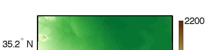
20 Table 2.1. Times (LST) of astronomical (ast) sunrise (SR) and sunset (ST), theoretical SR and ST of extraterrestrial (ext) radiation, and local (loc) SR and ST at four different sites in the Meteor Crater on 21 October Site RIM is located on the west rim of the crater (unobstructed by the surrounding topography), FLR in the center of the crater, and WU (22.7 slope angle) and EU (24.1 slope angle) on the west and east sidewall, respectively. Values are taken from Hoch and Whiteman (2010). ast SR ext SR loc SR ast ST ext ST loc ST RIM FLR WU EU It shows shortwave downward radiation at 0800 and 0930 LST for an idealized basin similar to the Meteor Crater from a WRF (Weather Research and Forecasting) model simulation that accounts only for self-shading (Figs. 2.1a,c) and one simulation that accounts for both self-shading and topographic shading (Figs. 2.1b,d). Both simulations produce a radiation maximum on the northwest sidewall, which faces the sun directly during the morning hours, while a shadow is present on the southeast sidewall, facing away from the sun. If neither self-shading nor topographic shading were taken into account, the shortwave incoming radiation field would be almost homogeneous throughout the domain with values identical to the values over the plain surrounding the basin in Fig Radiation values would vary slightly over the basin due to variations in the depth of the atmosphere and, thus, the attenuation of the incoming solar beam. Considering topographic effects, a shadow is thrown by the surrounding crater rim in the simulation with topographic shading at 0800 LST (Fig. 2.1b), which shades a large part of the basin floor resulting in lower radiation values than for the simulation without topographic shading (Fig. 2.1a). At 0930 LST, the length of the shadow thrown by the southeast rim has decreased (Fig. 2.1d) resulting in little difference between the simulation with and without topographic shading. Strongest

21 12 (a) 9 Self shading, 0800 LST 1000 (b) Self & topo shading, 0800 LST S N distance (km) R SW (W m 2 ) S N distance (km) R SW (W m 2 ) W E distance (km) (c) Self shading, 0930 LST W E distance (km) (d) Self & topo shading, 0930 LST S N distance (km) R SW (W m 2 ) S N distance (km) R SW (W m 2 ) W E distance (km) W E distance (km) Fig Shortwave incoming radiation (W m 2 ) at (a,b) 0800 LST and (c,d) 0930 LST from a WRF simulation that accounts for (a,c) self-shading and (b,d) self-shading and topographic shading. 0

22 13 effects are therefore seen in the early morning (and analogously in the late afternoon), when solar elevation is low. Terrain also affects other components of the radiation balance besides direct solar radiation. Shortwave radiation reflected by the terrain adds to diffuse sky radiation to enhance total diffuse radiation (Hoch and Whiteman 2010). Similarly, longwave radiation emitted from the topography adds to longwave incoming radiation from the atmosphere (Whiteman et al. 1989a; Hoch and Whiteman 2010). Longwave outgoing radiation depends on the surface temperature and is therefore affected by asymmetric heating of opposing mountain sidewalls (Whiteman et al. 1989a). Additional variations in radiation components result also from heterogeneities in soil and vegetation properties, affecting albedo and emissivity, and terrain elevation. Observations by Whiteman et al. (1989a) and Matzinger et al. (2003), respectively, have shown that daytime net radiation and spatial variations in net radiation are mostly determined by direct radiation and variations in global radiation. The timing of maximum net radiation in the Meteor Crater is also affected by the timing of maximum shortwave incoming radiation, resulting in a maximum on the west sidewall in the morning and a maximum on the east sidewall in the afternoon (Hoch and Whiteman 2010). Asymmetric net radiation affects other components of the surface energy budget. Whiteman et al. (1989b) found that both the sensible and latent heat fluxes reached their maximum values in the morning on the northeast-facing slope and in the afternoon on the southwest-facing slope. The sensible heat flux difference across the valley, with higher values on the west side before 1130 LST and higher values on the east side after 1130 LST, resulted in a cross-valley flow that was described by Whiteman (1989) and modeled by Bader and Whiteman (1989). In addition to radiation effects, variations in surface characteristics, such as vegetation type and coverage or soil moisture, can contribute to spatial inhomogeneities in the surface energy budget in mountainous terrain.

23 Asymmetric boundary-layer and thermal-wind formation Spatial variations in solar irradiation and sensible heat flux impact the development of the boundary layer and the formation of diurnal thermally driven wind systems, as observed in several previous studies. Reiter et al. (1983) performed pilot balloon soundings in the Loisach Valley, Germany, to observe the cross-valley asymmetries in the evolution of the valley wind system. They found an earlier onset of the evening down-valley wind near the west side of the north south aligned valley. They also described observations from the Inn Valley, Austria, which showed a similar earlier onset of the morning up-valley wind near the sunlit side. Lidar measurements in the Brush Creek Valley by Post and Neff (1986) revealed a displacement of the daytime up-valley flow toward the more strongly heated sidewall, but also a displacement of the nocturnal drainage flow to the east sidewall, which they hypothesized was caused by the curvature of the valley. Aerosol lidar measurements by Carnuth and Trickl (2000) in the Mesolcina Valley, Switzerland, showed higher aerosol concentrations and a deeper boundary layer over the west-facing sidewall in the afternoon. The authors also hypothesized that this asymmetry was produced either by stronger insolation of the west-facing sidewall or by centrifugal forces due to a bend in the valley. Observations in the Riviera Valley, Switzerland, during MAP (Mesoscale Alpine Program), on the other hand, showed a rather homogeneous temperature field across the valley (De Wekker et al. 2005). The authors speculated that strong mixing on this very convective measurement day could have reduced cross-valley temperature differences. Observed up-valley winds also showed maximum wind speeds constantly on the east side, whereas their model simulations produced a shift of the up-valley wind maximum from the west to the east sidewall, most likely due to the differential heating of the sidewalls. In a similar way, two-dimensional simulations by Bader and McKee (1983, 1985) and Bader and Whiteman (1989) produced symmetric tempera-

24 15 ture fields despite asymmetric heating of the valley sidewalls. They, too, argued that cross-valley mixing reduces horizontal temperature differences. As a second mixing mechanism they suggested gravity waves that form in the stable valley atmosphere. As a consequence, simulations by Bader and McKee (1985) showed little impact of the valley orientation on the valley boundary layer development. Asymmetric irradiation on opposing mountain sidewalls may also result in an asymmetric reversal of slope winds from downslope to upslope in the morning and from upslope to downslope in the evening if one sidewall is shaded from irradiation, while the other sidewall is illuminated. Buettner and Thyer (1966) measured the along-valley-wind system near Mount Rainier, Washington, and observed a balloon being carried down the shaded sidewall and up the opposite sunlit sidewall shortly after sunrise. ARPS (Advanced Regional Prediction System) simulations for a north south aligned idealized valley by Colette et al. (2003) showed that asymmetric heating of the west and east sidewalls in the morning leads to an asymmetric growth of the convective boundary layer (CBL) across the valley and to variations in the onset of upslope winds. LES of the evolution of the valley boundary layer in a north south oriented valley by Anquetin et al. (1998) using Submeso (based on ARPS) produced similar results, with an asymmetric development of upslope and downslope winds in the morning and evening, respectively, and strong vertical motions near the sunny sidewall. The CBL depth, however, varied across the valley only in a winter case, whereas the top of the CBL was horizontally homogeneous in their summer case. Kelly (1988) observed an asymmetric inversion breakup in the approximately north south aligned Laramie Valley, Wyoming. He described how the morning inversion breakup and the transition from nocturnal drainage winds to first upslope flows and then to the regional winds that are mixed down from aloft started near the west sidewall and propagated toward the east. Morning tracer experiments in the Brush Creeek Valley produced a tracer trans-

25 16 port up the west, sunlit sidewall after sunrise resulting in an asymmetric tracer distribution about the valley axis with maximum concentrations on the southwest sidewall and only weak concentrations on the opposite northeast sidewall (Gudiksen and Shearer 1989; Orgill 1989). Similarly, Lehner and Gohm (2010) found for an idealized valley that upslope winds developed earlier on the sunlit sidewall in the morning, while katabatic flows still persisted on the shaded sidewall resulting in a transport of air pollutants up the sunlit sidewall. Asymmetric irradiation not only affects the timing of slope-wind reversal, but can also affect the strength of the developing upslope winds on opposite sidewalls. Segal et al. (1987) determined the upslope-flow speed on a north- and a south-facing slope for varying slope angles and time of the year. They found that a stronger and deeper flow developed on the south-facing slope compared with the north-facing slope and that this difference was most pronounced during the winter season and at high latitudes Thermally driven cross-valley flows Early observations of diurnal thermally driven cross-valley flows date back to the first half of the last century. Moll (1935) conducted pilot balloon soundings in four valleys in Tyrol, Austria, in which he observed morning cross-valley flows toward the sunlit sidewall above the along-valley wind system. In North America, MacHattie (1968) observed surface cross-valley winds in the Kananaskis Valley, Canada, and found that the cross-valley winds had more pronounced diurnal variations than the along-valley flow. An overview of studies on thermally generated and dynamically generated cross-valley winds before the second half of the 1980s is given by Hennemuth (1986). Urfer-Henneberger (1970) modified Defant s (1949) diagram of the diurnal valley and slope wind circulation to add information on cross-valley flows based on observations from the Dischma Valley, Switzerland. The new diagram in-

26 17 cluded morning and evening asymmetries in the across-valley direction, with a morning cross-valley flow below the down-valley wind, which does not reach the surface, and an evening cross-valley flow above the down-valley wind. Observations of cross-valley flows in the Dischma Valley are found in research papers by Hennemuth and Schmidt (1985), Hennemuth (1986), and Urfer-Henneberger (1970). Hennemuth and Schmidt (1985) observed cross-valley flows that were most pronounced in the morning when along-valley flows were weak. In the afternoon the presence of a strong along-valley wind led instead to the deflection of the along-valley wind in the cross-valley direction. Hennemuth (1986) reported cross-valley winds with wind speeds of up to 5 m s 1. Her calculation of the heat budget for the Dischma Valley revealed that the cross-valley flow reduced the cross-valley temperature difference, but that it did not affect the heat budget of the entire valley since it led only to a redistribution of heat within the valley cross section. Hennemuth also suggested that the diurnal thermally driven cross-valley winds interacted with dynamically induced winds produced by the flow above ridge level. Early idealized simulations of the valley wind system with a three-dimensional model (Egger 1981) produced cross-valley winds with a weak return flow aloft when only one sidewall was heated. Later simulations for the Riviera Valley, Switzerland, with a more sophisticated mesoscale numerical model by De Wekker et al. (2005) also showed a morning cross-valley flow toward the more sunlit sidewall. Their observations from the Riviera Valley, however, showed rather a deflection of the up-valley wind. But simulations by Weigel et al. (2006) for the Riviera Valley showed again an afternoon thermal cross-valley circulation in the northern part of the valley. Gleeson (1951), in his theoretical study, calculated cross-valley winds from the equations of horizontal motion, considering pressure-gradient force, Coriolis force, and friction. He parameterized the cross-valley temperature gradient with the difference in incoming radiation, neglecting other effects such as advection by the developing cross-

27 18 valley flow, which would reduce the temperature gradient. Gleeson found qualitatively good agreement between his theoretical results and observations from the Columbia River Valley, British Columbia. He also used his set of equations to study the effects of inertia, latitude, slope inclination, season, and valley orientation on the crossvalley flow and discovered that strongest winds can occur at a latitude of 30 and that higher wind speeds can occur in valleys with steeper slopes because of larger radiation differences between the sidewalls. The impact of cross-valley flows on air pollution transport was mentioned by Whiteman (1989), who performed tracer experiments in the Brush Creek Valley during the morning period after sunrise. Cross-valley winds formed between the sunlit southwest and the shaded northeast sidewall, which transported the tracer toward the southwest side leading to asymmetric tracer concentrations about the valley axis. The author hypothesized that the formation of cross-valley flows is favored in the Brush Creek Valley due to its small width, the northwest southeast orientation that allows for strong differential heating of the sidewalls in the morning, and the semiarid climate that leads to large sensible heat fluxes. He also called for further studies investigating the effect of valley orientation and width on the cross-valley circulation. Bader and Whiteman (1989) performed two-dimensional model simulations of tracer dispersion in a northwest southeast aligned valley and compared their results with the observations by Whiteman (1989). In their summer case, the tracer plume was transported toward the sunlit southwest sidewall, similar to the observations. In their winter case, however, tracer dispersion is more symmetric about the valley axis because differences in heating between the sidewalls are smaller than in summer Dynamically induced cross-valley flows Cross-valley winds can also be generated dynamically without thermal forcing. Some of the main dynamic mechanisms producing cross-valley winds are summarized

28 19 here. If strong synoptic winds are present with a wind direction normal to the valley axis, synoptic winds can penetrate into the valley following the topography so that the wind direction in the valley is identical to the wind direction above the valley (Egger 2003). Bell and Thompson (1980) performed numerical simulations and water-tank experiments and determined a critical Froude number, above which synoptic winds can penetrate into the valley. Cross-valley winds produced by the large-scale flow penetrating into the valley can also be related to downslope windstorm events as observed and simulated in the Owens Valley, California, by Jiang and Doyle (2008). Cross-valley winds induced by the curvature of the valley are described by Weigel and Rotach (2004) and Weigel et al. (2006) for the Riviera Valley, Switzerland. Observations during MAP revealed an asymmetry of the up-valley flow in the southern part of the valley, with a jet maximum near the east sidewall, and a closed cross-valley circulation with a downslope flow on the sun-exposed, west-facing sidewall above a shallow upslope-flow layer. Weigel and Rotach (2004) explain this phenomenon as a secondary circulation produced by the valley curvature. As the flow from the upstream Magadino Valley enters the Riviera Valley it must go around a sharp corner. The resulting centrifugal forces push the flow to the east side, which explains the jet maximum near this sidewall. Due to the cold air from upstream being pushed up the east sidewall a cross-valley pressure gradient forms, which opposes the centrifugal force. Since the up-valley wind increases with height due to surface friction, the centrifugal force also increases with height so that the centrifugal force is larger than the pressure-gradient force at the top, but lower than the pressure-gradient force near the valley floor. The result is a closed cross-valley circulation with a component away from the east sidewall near the valley floor and a component toward the east sidewall near the top. LES by Weigel et al. (2006) produced the same result in the southern part of the Riviera Valley, but also a thermal cross-valley circulation in the northern part of the valley in the afternoon, with an anabatic wind on the west-facing, sun-

29 20 exposed sidewall and a katabatic wind on the east-facing sidewall. They concluded that the secondary circulation induced by the valley curvature must be stronger than the thermally induced circulation to result in the reversed cross-valley circulation observed in the southern part of the valley. Other local winds can intrude into a valley to produce cross-valley flows. Banta et al. (2004) observed nighttime slope flows and canyon exit jets along the Wasatch Mountains to the east of the Salt Lake Basin that reached some distance into the basin resulting in a local flow in the cross-valley direction. Vergeiner and Dreiseitl (1987) postulated that the mass flux in the upslope-wind layer is inversely proportional to the vertical potential temperature gradient in the valley atmosphere. According to their conceptual model, the mass flux in the slopewind layer is therefore reduced within an elevated inversion layer compared with the atmosphere below and above. If mass is conserved within the valley cross section, cross-valley circulations are expected to develop with a flow away from the slope at the bottom boundary of the inversion layer and a flow toward the slope at the top boundary. Such cross-valley flows induced by elevated inversion layers have been observed in the Inn Valley, Austria (Gohm et al. 2009; Harnisch et al. 2009) and have been reproduced with idealized numerical simulations (Lehner and Gohm 2010). The same effect can be produced by surface inhomogeneities along the upslope-wind sidewall (Shapiro and Fedorovich 2007; Lehner and Gohm 2010). In section 3.7 data from the Meteor Crater are analyzed from a 1-h morning period with an elevated inversion layer and an elevated cross-basin flow is found to be in agreement with the conceptual model by Vergeiner and Dreiseitl (1987). 2.3 METCRAX The Meteor Crater Experiment (METCRAX) was a one-month-long field campaign that took place in the Meteor Crater, Arizona (Fig. 2.2), during October 2006

30 21 Fig Arizona s Meteor Crater. Picture taken from the visitor center. (Whiteman et al. 2008). The initial focus of METCRAX was on the investigation of stable boundary layer evolution, seiches, and internal waves in the nocturnal stable layer. The Meteor Crater was chosen as an almost ideal site for this experiment because of its almost circular, bowl-shaped topography. The Meteor Crater ( W, N), also known as Barringer Meteorite Crater, is located approximately 40 km east of Flagstaff, Arizona (Fig. 2.3a). It was produced by the impact of a m-diameter meteorite about 49,000 50,000 years ago (Kring 2007). The crater basin is 180 m deep and 1200 m in diameter at the height of the crater rim with an 500 m wide crater floor (Fig. 2.3c). The crater sidewalls are steepest in the upper part of the crater with average slope angles of The crater rim extends about m above the surrounding plain located on the Colorado Plateau, which slopes gently upward at an angle of 1 toward the Mogollan Rim to the southwest of the crater. A detailed description of the instruments deployed during the field campaign is given in the METCRAX overview paper by Whiteman et al. (2008). Additional information on the instruments supplied by the National Center for Atmospheric Research (NCAR) can be found online ( and Most of the instruments were operated continuously throughout the entire field campaign. Additional measurements, includ-

31 22 (a) (b) (c) Fig Location and topography of Arizona s Meteor Crater. (a) Location of the Meteor Crater in Arizona, (b) Meteor Crater and surroundings, and (c) detailed view of the Meteor Crater basin.

32 23 ing tethersonde ascents inside the crater and rawinsonde launches in the vicinity of the crater, were performed during seven IOPs (intensive observational periods) between mid-afternoon and mid-morning. The data used for the observational part of this study (Chapter 3) are described in section 3.3. Several studies have since made use of the extensive METCRAX dataset contributing to research both within and outside the initial focus of the program. METCRAX observations were used to investigate the impact of synoptic and local winds above the crater basin and of static stability outside the crater on the formation of nocturnal inversions inside the crater (Yao and Zhong 2009). Hahnenberger (2008) tested the applicability of the topographic-amplification-factor concept to the Meteor Crater by comparing the diurnal heating and cooling inside the crater basin and over the surrounding plain. Turbulence characteristics at a site inside the crater were compared with a site outside the crater by Fu et al. (2010). Fritts et al. (2010) used a spectral-element model to simulate the response of the crater atmosphere in an idealized axisymmetric crater to flow of 2 8 m s 1 above the crater. Topographic effects on the radiation components in the Meteor Crater were investigated by Hoch and Whiteman (2010) and Hoch et al. (2011). Hoch and Whiteman (2010) reported measurements of radiation balance components at several sites in the crater basin and Hoch et al. (2011) used a three-dimensional radiative transfer model to estimate the contribution of longwave radiative cooling and heating to the total nocturnal temperature tendency in the Meteor Crater. Savage et al. (2008) used observations together with numerical simulations to study the strength, depth, and spatial distribution of a nocturnal downslope flow that develops on the slightly sloping plain surrounding the crater. Whiteman et al. (2010) discovered that the mesoscale drainage flow leads to the build-up of a cold-air pool upwind of the crater rim and that the cold air then spills into the crater, where it flows down the inner crater sidewall until it reaches its level of neutral buoyancy. The inflow

33 24 of cold air destabilizes the nocturnal crater atmosphere leading to a near-isothermal layer above a shallow inversion near the crater floor. The cold-air intrusions were modeled using a simple mass-flux model to determine the mechanisms that produce the near-isothermal layer by Haiden et al. (2011). Kiefer and Zhong (2011) used a mesoscale numerical model to examine the influence of topographic parameters such as basin size and the presence of a crater rim on the evolution of cold-air intrusions and the formation of the near-isothermal layer. Adler et al. (2012) found that changes in the mesoscale drainage flow can produce a thickening of the cold-air layer that flows into the crater resulting in intermittent downslope-windstorm-like flows on the upstream inner crater sidewall with increased wind speeds and intrusions of warmer air from further aloft. The Meteor Crater provides a nearly ideal location for studying the diurnal thermally driven cross-valley circulation because of its size and almost circular topography. The small basin allows for the formation of relatively strong cross-basin temperature gradients from asymmetric irradiation, which can produce measurable cross-basin flows. In addition, due to the circular basin topography cross-basin flows can be observed throughout the entire day with a direction that changes as the sun moves across the sky, from easterly in the morning, over southerly around noon, to westerly in the evening (see section 3.4). A photograph illustrating asymmetric irradiation in the Meteor Crater is shown in Fig In the photograph, one sidewall is illuminated while the other sidewall is in shadow. 2.4 WRF and LES in mountainous terrain High-resolution modeling in mountainous terrain Axelsen and van Dop (2009a) gave a short overview of slope flow simulation studies performed with RANS (Reynolds Averaged Navier-Stokes), LES, and DNS (Direct Numerical Simulation) models. Pioneering LES work of slope winds was done by

34 25 Fig Asymmetric irradiation in the Meteor Crater. Picture taken from the northwest. Photo Sebastian Hoch. Schumann (1990), who performed simulations of the convective boundary layer over an inclined surface. Several simulations of the nighttime katabatic flow have been performed since and compared with observations or results from mesoscale models (Axelsen and van Dop 2009a, 2009b; Skyllingstad 2003; Smith and Skyllingstad 2005). LES models have also been used to study flow over mountains (Smith and Skyllingstad 2009, 2011). An outlook on LES as a new tool for studies of flow over complex terrain was given more than ten years ago by Wood (2000). The ARPS model and models based on it have been used frequently for LES modeling studies over complex terrain with various horizontal grid spacings in the range of 150 to 350 m (e.g., Guilbaud et al. 1997; Anquetin et al. 1998, 1999; Chen et al. 2004; Chow et al. 2006; Weigel et al. 2006, 2007b, 2007a; Schmidli et al. 2009), but also down to 25 to 50 m (e.g., Michioka and Chow 2008; Chow and Street 2009; Serafin and Zardi 2010b, 2010a, 2011). Other typically mesoscale models have been used as well for LES studies in complex terrain, such as WRF (Catalano and Cenedese 2010; Catalano and Moeng 2010) or RAMS (Regional Atmospheric Modeling System; Walko et al. 1992). An important requirement for modeling the cross-valley or cross-basin circulation is that the radiation parameterization accounts for both self-shading and topographic shading in order to reproduce the asymmetric irradiation effects correctly. While shading is absolutely necessary in modeling cross-valley winds, studies with several

35 26 different models have shown that shading is generally important for high-resolution simulations in mountainous terrain. Colette et al. (2003) implemented a topographicshading routine in ARPS. Their simulations showed that upslope-wind formation and inversion breakup in steep valleys can be delayed by topographic shading. For MM5 (Mesoscale Model version 5), Hauge and Hole (2003) improved the agreement of modeled temperature and wind speed with observations using a modified radiation scheme that included self-shading compared to the original radiation scheme without self-shading. Similarly, Manners et al. (2012) implemented a new surface radiation parameterization that accounts for self-shading and topographic shading in the MetUM (Met Office Unified Model). Their tests for different locations in Scotland and England resulted in temperature differences due to terrain effects, as well as in improved precipitation forecasts The Weather Research and Forecasting model Simulations for this study were run with the Weather Research and Forecasting (WRF) model version 3.2.1, more specifically with the Advanced Research WRF (ARW) dynamics solver developed at NCAR. WRF is used both operationally and in research, offering the user different options concerning, for example, physics parameterizations, boundary conditions, nesting, and spatial discretization (Skamarock et al. 2008). A detailed description of the respective model setup for the simulations is given at the beginning of the chapters presenting the numerical results (Chapters 4 and 5). General information on the ARW dynamic solver can be found in Skamarock and Klemp (2008) and in the ARW technical description (Skamarock et al. 2008). The latter also describes the WRF software, the different physics parameterizations, boundary conditions, and other model options. A description of the software framework is given by Michalakes et al. (2005) together with performance results from benchmark simulations with version 2. The ARW solves the compressible nonhy-

36 27 drostatic equations in flux form using a third-order Runge-Kutta time integration scheme. The time-split method used to integrate in time is described by Klemp et al. (2007). The spatial discretization in WRF is done on a staggered Arakawa C-grid and the vertical coordinate is a terrain-following pressure coordinate. In LES configuration, WRF is run with a grid spacing that is small enough ( x 100 m) to explicitly resolve the large, most energy-containing turbulent motions. The effects of motions of scales smaller than the grid spacing on the resolved motions are parameterized with a subgrid-scale (or subfilter-scale) turbulence model. For users, the transition from a mesoscale simulation to LES means that the model is set up to run without a PBL (planetary boundary layer) parameterization, which handles vertical mixing throughout the atmosphere for larger-scale simulations, and that the two-dimensional horizontal mixing parameterization is replaced with a three-dimensional subgrid-scale turbulence model. WRF version 3 offers two threedimensional turbulence-model options: a Smagorinsky model (Smagorinsky 1963) and a 1.5-order TKE (turbulence kinetic energy) model (Deardorff 1980). The number of LES studies with WRF has been growing continuously during recent years. Applications of WRF LES are manifold: studies of, for example, seabreeze circulations (Antonelli and Rotunno 2007), hurricane boundary layers (Zhu 2008), tropical cyclones (Rotunno et al. 2009), and marine stratocumulus clouds (Wang and Feingold 2009); tests of the applicability of two-way nesting for LES (Moeng et al. 2007); the evaluation of the order of spatial differencing in advection schemes for cloud modeling (Wang et al. 2009); and the comparison of turbulent statistics over flat terrain from LES with a PBL parameterization (Hattori et al. 2010). Catalano and Cenedese (2010) and Catalano and Moeng (2010) ran WRF LES over mountainous terrain in their respective studies of the diurnal cycle of the slope wind circulation and the boundary layer evolution in an idealized valley. Recently, studies were presented that worked toward an improvement of LES performance with

37 28 WRF. Lundquist et al. (2010) implemented an immersed boundary method to reduce numerical errors near steep terrain, which are inherent to terrain-following vertical coordinates, and tested it over terrain as complicated as an urban setting. Mirocha et al. (2010) added a nonlinear subfilter-scale stress model and tested it against the standard WRF Smagorinsky and 1.5-order TKE models, while Kirkil et al. (2012) implemented two dynamic subfilter-scale turbulence models and tested them against the standard WRF Smagorinsky model and the nonlinear subfilter-scale stress model by Mirocha et al. (2010). 2.5 References Adler, B., C. D. Whiteman, S. W. Hoch, M. Lehner, and N. Kalthoff, 2012: Warm-air intrusions in Arizona s Meteor Crater. J. Appl. Meteor. Climatol., 51, Anquetin, S., C. Guilbaud, and J.-P. Chollet, 1998: The formation and destruction of inversion layers within a deep valley. J. Appl. Meteor., 37, Anquetin, S., C. Guilbaud, and J.-P. Chollet, 1999: Thermal valley inversion impact on the dispersion of a passive pollutant in a complex mountainous area. Atmos. Environ., 33, Antonelli, M., and R. Rotunno, 2007: Large-eddy simulation of the onset of the sea breeze. J. Atmos. Sci., 64, Axelsen, S. L., and H. van Dop, 2009a: Large-eddy simulation of katabatic winds. Part 1: Comparison with observations. Acta Geophys., 57, Axelsen, S. L., and H. van Dop, 2009b: Large-eddy simulation of katabatic winds. Part 2: Sensitivity study and comparison with analytical models. Acta Geophys., 57, Bader, D. C., and T. B. McKee, 1983: Dynamical model simulation of the morning boundary layer development in deep mountain valleys. J. Climate Appl. Meteor., 22, Bader, D. C., and T. B. McKee, 1985: Effects of shear, stability and valley characteristics on the destruction of temperature inversions. J. Climate Appl. Meteor., 24, Bader, D. C., and C. D. Whiteman, 1989: Numerical simulation of cross-valley plume

38 dispersion during the morning transition period. J. Appl. Meteor., 28, Banta, R., and W. R. Cotton, 1981: An analysis of the structure of local wind systems in a broad mountain basin. J. Appl. Meteor., 20, Banta, R. M., L. S. Darby, J. D. Fast, J. O. Pinto, C. D. Whiteman, W. J. Shaw, and B. W. Orr, 2004: Nocturnal low-level jet in a mountain basin complex. Part I: Evolution and effects on local flows. J. Appl. Meteor., 43, Barr, S., and M. M. Orgill, 1989: Influence of external meteorology on nocturnal valley drainage winds. J. Appl. Meteor., 28, Bell, R. C., and R. O. R. Y. Thompson, 1980: Valley ventilation by cross winds. J. Fluid Mech., 96, Buettner, K. J. K., and N. Thyer, 1966: Valley winds in the Mount Rainier area. Arch. Meteor. Geophys. Bioklimatol., B14, Carnuth, W., and T. Trickl, 2000: Transport studies with the IFU three-wavelength aerosol lidar during the VOTALP Mesolcina experiment. Atmos. Environ., 34, Catalano, F., and A. Cenedese, 2010: High-resolution numerical modeling of thermally driven slope winds in a valley with strong capping. J. Appl. Meteor. Climatol., 49, Catalano, F., and C.-H. Moeng, 2010: Large-eddy simulation of the daytime boundary layer in an idealized valley using the Weather Research and Forecasting numerical model. Bound.-Layer Meteor., 137, Chen, Y., F. L. Ludwig, and R. L. Street, 2004: Stably stratified flows near a notched transverse ridge across the Salt Lake Valley. J. Appl. Meteor., 43, Chow, F. K., and R. L. Street, 2009: Evaluation of turbulence closure models for large-eddy simulation over complex terrain: Flow over Askervein Hill. J. Appl. Meteor. Climatol., 48, Chow, F. K., A. P. Weigel, R. L. Street, M. W. Rotach, and M. Xue, 2006: Highresolution large-eddy simulations of flow in a steep Alpine valley. Part I: Methodology, verification, and sensitivity experiments. J. Appl. Meteor. Climatol., 45, Colette, A., F. K. Chow, and R. L. Street, 2003: A numerical study of inversionlayer breakup and the effects of topographic shading in idealized valleys. J. Appl. Meteor., 42, De Wekker, S. F. J., K. S. Godwin, G. D. Emmitt, and S. Greco, 2012: Airborne 29

39 Doppler lidar measurements of valley flows in complex coastal terrain. J. Appl. Meteor. Climatol., 51, De Wekker, S. F. J., D. G. Steyn, J. D. Fast, M. W. Rotach, and S. Zhong, 2005: The performance of RAMS in representing the convective boundary layer structure in a very steep valley. Environ. Fluid Mech., 5, Deardorff, J. W., 1980: Stratocumulus-capped mixed layers derived from a threedimensional model. Bound.-Layer Meteor., 18, Defant, F., 1949: Zur Theorie der Hangwinde, nebst Bemerkungen zur Theorie der Berg- und Talwinde [On the theory of slope winds, along with remarks on the theory of mountain and valley winds]. Arch. Meteor. Geophys. Bioklimatol., A1, , [English translation in Whiteman, C.D., and E. Dreiseitl, 1984: Alpine Meteorology. Translations of Classic Contributions by A. Wagner, E. Ekhart and F. Defant. PNL-5141, ASCOT-84-3, Pacific Northwest Laboratory, Richland, WA, 121 pp.]. Egger, J., 1981: Thermally forced circulations in a valley. Geophys. Astrophys. Fluid Dyn., 17, Egger, J., 1990: Thermally forced flows: Theory. Atmospheric Processes over Complex Terrain. Meteor. Monogr., Amer. Meteor. Soc., No. 45, Egger, J., 2003: Valley winds. Encyclopedia of Atmospheric Sciences, Elsevier Science Ltd., Egger, J., S. Bajrachaya, U. Egger, R. Heinrich, J. Reuder, P. Shayka, H. Wendt, and V. Wirth, 2000: Diurnal winds in the Himalayan Kali Gandaki Valley. Part I: Observations. Mon. Wea. Rev., 128, Fleagle, R. G., 1950: A theory of air drainage. J. Meteor., 7, Fritts, D. C., D. Goldstein, and T. Lund, 2010: High-resolution numerical studies of stable boundary layer flows in a closed basin: Evolution of steady and oscillatory flows in an axisymmetric Arizona Meteor Crater. J. Geophys. Res., 115, D Fu, P., S. Zhong, C. D. Whiteman, T. Horst, and X. Bian, 2010: An observational study of turbulence inside a closed basin. J. Geophys. Res., 115, D Gleeson, T. A., 1951: On the theory of cross-valley winds arising from differential heating of the slopes. J. Meteor., 8, Gohm, A., and Coauthors, 2009: Air pollution transport in an Alpine valley: Results from airborne and ground-based observations. Bound.-Layer Meteor., 131,

40 Grisogono, B., and J. Oerlemans, 2001: Katabatic flow: Analytic solution for gradually varying eddy diffusivities. J. Atmos. Sci., 58, Gudiksen, P. H., J. M. Leone, C. W. King, D. Ruffieux, and W. D. Neff, 1992: Measurements and modeling of the effects of ambient meteorology on nocturnal drainage flows. J. Appl. Meteor., 31, Gudiksen, P. H., and D. L. Shearer, 1989: The dispersion of atmospheric tracers in nocturnal drainage flows. J. Appl. Meteor., 28, Guilbaud, C., J. P. Chollet, and S. Anquetin, 1997: Large eddy simulations of stratified atmospheric flows within a deep valley. Direct and Large-Eddy Simulation II, J.-P. Chollet et al., Ed., Kluwer Academic Publishers, Hahnenberger, M., 2008: Topographic effects on nighttime cooling in a basin and plain atmosphere. M.S. thesis, Dept. of Meteorology, University of Utah, 85 pp. Haiden, T., C. D. Whiteman, S. W. Hoch, and M. Lehner, 2011: A mass flux model of nocturnal cold-air intrusions into a closed basin. J. Appl. Meteor. Climatol., 50, Harnisch, F., A. Gohm, A. Fix, R. Schnitzhofer, A. Hansel, and B. Neininger, 2009: Spatial distribution of aerosols in the Inn Valley atmosphere during wintertime. Meteor. Atmos. Phys., 103, Hattori, Y., C.-H. Moeng, H. Hirakuchi, S. Ishihara, S. Sugimoto, and H. Suto, 2010: Numerical simulation of turbulence structures in the neutral-atmospheric surface layer with a mesoscale meteorological model, WRF. The Fifth International Symposium on Computational Wind Engineering, Chapel Hill, NC. Hauge, G., and L. R. Hole, 2003: Implementation of slope irradiance in Mesoscale Model version 5 and its effect on temperature and wind fields during the breakup of a temperature inversion. J. Geophys. Res., 108(D2), Hennemuth, B., 1986: Thermal asymmetry and cross-valley circulation in a small Alpine valley. Bound.-Layer Meteor., 36, Hennemuth, B., and H. Schmidt, 1985: Wind phenomena in the Dischma Valley during DISKUS. Arch. Meteor. Geophys. Bioklimatol., B35, Hoch, S. W., and C. D. Whiteman, 2010: Topographic effects on the surface radiation balance in and around Arizona s Meteor Crater. J. Appl. Meteor. Climatol., 49, Hoch, S. W., C. D. Whiteman, and B. Mayer, 2011: A systematic study of longwave radiative heating and cooling within valleys and basins using a three-dimensional 31

41 32 radiative transfer model. J. Appl. Meteor. Climatol., 50, Horst, T. W., and J. C. Doran, 1988: The turbulence structure of nocturnal slope flow. J. Atmos. Sci., 45, Hunt, J. C. R., H. J. S. Fernando, and M. Princevac, 2003: Unsteady thermally driven flows on gentle slopes. J. Atmos. Sci., 60, Jiang, Q., and J. D. Doyle, 2008: Diurnal variation of downslope winds in Owens Valley during the Sierra Rotor Experiment. Mon. Wea. Rev., 136, Kelly, R. D., 1988: Asymmetric removal of temperature inversions in a high mountain valley. J. Appl. Meteor., 27, Kiefer, M. T., and S. Zhong, 2011: An idealized modeling study of nocturnal cooling processes inside a small enclosed basin. J. Geophys. Res., 116, D Kirkil, G., J. Mirocha, E. Bou-Zeid, F. K. Chow, and B. Kosović, 2012: Implementation and evaluation of dynamic subfilter-scale stress models for large-eddy simulation using WRF. Mon. Wea. Rev., 140, Klemp, J. B., W. C. Skamarock, and J. Dudhia, 2007: Conservative split-explicit time integration methods for the compressible nonhydrostatic equations. Mon. Wea. Rev., 135, Kring, D. A., 2007: Guidebook to the Geology of Barringer Meteorite Crater, Arizona (aka Meteor Crater): Fieldguide for the 70th Annual Meeting of the Meteoritical Society. LPI Contribution 1355, Lunar and Planetary Institute, Houston, TX, 150 pp. Lehner, M., and A. Gohm, 2010: Idealised simulations of daytime pollution transport in a steep valley and its sensitivity to thermal stratification and surface albedo. Bound.-Layer Meteor., 134, Leone, J. M., and R. L. Lee, 1989: Numerical simulation of drainage flow in Brush Creek, Colorado. J. Appl. Meteor., 28, Lundquist, K. A., F. K. Chow, and J. K. Lundquist, 2010: An immersed boundary method for the Weather Research and Forecasting model. Mon. Wea. Rev., 138, MacHattie, L. B., 1968: Kananaskis valley winds in summer. J. Appl. Meteor., 7, Manins, P. C., and B. L. Sawford, 1979a: Katabatic winds: A field case study. Quart. J. Roy. Meteor. Soc., 105,

42 Manins, P. C., and B. L. Sawford, 1979b: A model of katabatic winds. J. Atmos. Sci., 36, Manners, J., S. B. Vosper, and N. Roberts, 2012: Radiative transfer over resolved topographic features for high-resolution weather prediction. Quart. J. Roy. Meteor. Soc., 138, Matzinger, N., M. Andretta, E. van Gorsel, R. Vogt, A. Ohmura, and M. W. Rotach, 2003: Surface radiation budget in an Alpine valley. Quart. J. Roy. Meteor. Soc., 129, McKee, T. B., and R. D. O Neal, 1989: The role of valley geometry and energy budget in the formation of nocturnal valley winds. J. Appl. Meteor., 28, Michalakes, J., J. Dudhia, D. Gill, T. Henderson, J. Klemp, W. Skamarock, and W. Wang, 2005: The Weather Research and Forecast model: Software architecture and performance. Proc. 11 th ECMWF Workshop on the Use of High Performance Computing in Meteorology, W. Zwieflhofer and G. Mozdzynski, Eds., Michioka, T., and F. K. Chow, 2008: High-resolution large-eddy simulations of scalar transport in atmospheric boundary layer flow over complex terrain. J. Appl. Meteor. Climatol., 47, Mirocha, J. D., J. K. Lundquist, and B. Kosović, 2010: Implementation of a nonlinear subfilter turbulence stress model for large-eddy simulation in the Advanced Research WRF model. Mon. Wea. Rev., 138, Moeng, C.-H., J. Dudhia, J. Klemp, and P. Sullivan, 2007: Examining two-way grid nesting for large eddy simulation of the PBL using the WRF model. Mon. Wea. Rev., 135, Moll, E., 1935: Aerologische Untersuchung periodischer Gebirgswinde in V-förmigen Alpentälern [Aerological investigation of periodic mountain winds in V-shaped Alpine valleys]. Beitr. Phys. Atmos., 22, Orgill, M. M., 1989: Early morning ventilation of a gaseous tracer from a mountain valley. J. Appl. Meteor., 28, Orgill, M. M., J. D. Kincheloe, and R. A. Sutherland, 1992: Mesoscale influences of nocturnal valley drainage winds in western Colarodo valleys. J. Appl. Meteor., 31, Papadopoulos, K. H., C. G. Helmis, A. T. Soilemes, J. Kalogiros, P. G. Papgeorgas, and D. N. Asimakopoulos, 1997: The structure of katabatic flows down a simple slope. Quart. J. Roy. Meteor. Soc., 123,

43 Post, M. J., and W. D. Neff, 1986: Doppler lidar measurements of winds in a narrow mountain valley. Bull. Amer. Meteor. Soc., 67, Poulos, G., and S. Zhong, 2008: An observational history of small-scale katabatic winds in mid-latitudes. Geogr. Compass, 2, Poulos, G. S., J. E. Bossert, T. B. McKee, and R. A. Pielke, 2000: The interaction of katabatic flow and mountain waves. Part I: Observations and idealized simulations. J. Atmos. Sci., 57, Prandtl, L., 1942: Führer durch die Strömungslehre. F. Vieweg & Sohn Verlagsgesellschaft mbh, 648 pp. Princevac, M., and H. J. S. Fernando, 2007: A criterion for the generation of turbulent anabatic flows. Phys. Fluids, 19, Rampanelli, G., D. Zardi, and R. Rotunno, 2004: Mechanisms of up-valley winds. J. Atmos. Sci., 61, Reiter, R., H. Müller, R. Sladkovic, and K. Munzert, 1983: Aerologische Untersuchungen der tagesperiodischen Gebirgswinde unter besonderer Berücksichtigung des Windfeldes im Talquerschnitt [Aerological investigations of diurnal mountain winds with special consideration of the wind field in the valley cross section]. Meteorol. Rundsch., 36, Rotunno, R., Y. Chen, W. Wang, C. Davis, J. Dudhia, and G. J. Holland, 2009: Large-eddy simulation of an idealized tropical cyclone. Bull. Amer. Meteor. Soc., 90, Rucker, M., R. M. Banta, and D. G. Steyn, 2008: Along-valley structure of daytime thermally driven flows in the Wipp Valley. J. Appl. Meteor. Climatol., 47, Savage, L. C., S. Zhong, W. Yao, W. J. O. Brown, T. W. Horst, and C. D. Whiteman, 2008: An observational and numerical study of a regional-scale downslope flow in northern Arizona. J. Geophys. Res., 113, D Schmidli, J., G. S. Poulos, M. H. Daniels, and F. K. Chow, 2009: External influences on nocturnal thermally driven flows in a deep valley. J. Appl. Meteor. Climatol., 48, Schmidli, J., and R. Rotunno, 2010: Mechanisms of along-valley winds and heat exchange over mountainous terrain. J. Atmos. Sci., 67, Schmidli, J., and Coauthors, 2011: Intercomparison of mesoscale model simulations of the daytime valley wind system. Mon. Wea. Rev., 139, Schumann, U., 1990: Large-eddy simulation of the up-slope boundary layer. Quart. 34

44 35 J. Roy. Meteor. Soc., 116, Segal, M., Y. Ookouchi, and R. A. Pielke, 1987: On the effect of steep slope orientation on the intensity of daytime upslope flow. J. Atmos. Sci., 44, Serafin, S., and D. Zardi, 2010a: Daytime heat transfer processes related to slope flows and turbulent convection in an idealized mountain valley. J. Atmos. Sci., 67, Serafin, S., and D. Zardi, 2010b: Structure of the atmospheric boundary layer in the vicinity of a developing upslope flow system: A numerical model study. J. Atmos. Sci., 67, Serafin, S., and D. Zardi, 2011: Daytime development of the boundary layer over a plain and in a valley under fair weather conditions: A comparison by means of idealized numerical simulations. J. Atmos. Sci., 68, Shapiro, A., and E. Fedorovich, 2007: Katabatic flow along a differentially cooled sloping surface. J. Fluid Mech., 571, Skamarock, W. C., and J. B. Klemp, 2008: A time-split nonhydrostatic atmospheric model for weather research and forecasting applications. J. Comput. Phys., 227, Skamarock, W. C., and Coauthors, 2008: A description of the Advanced Research WRF version 3. Tech. Rep. NCAR/TN-475+STR. 113 pp. Skyllingstad, E. D., 2003: Large-eddy simulation of katabatic flows. Bound.-Layer Meteor., 106, Smagorinsky, J., 1963: General circulation experiments with the primitive equations. I: The basic experiment. Mon. Wea. Rev., 91, Smith, C. M., and E. D. Skyllingstad, 2005: Numerical simulation of katabatic flow with changing slope angle. Mon. Wea. Rev., 133, Smith, C. M., and E. D. Skyllingstad, 2009: Investigation of upstream boundary layer influence on mountain wave breaking and lee wave rotors using a large-eddy simulation. J. Atmos. Sci., 66, Smith, C. M., and E. D. Skyllingstad, 2011: Effects of inversion height and surface heat flux on downslope windstorms. Mon. Wea. Rev., 139, Steinacker, R., 1984: Area-height distribution of a valley and its relation to the valley wind. Beitr. Phys. Atmos., 57, Stiperski, I., I. Kavčič, B. Grisogono, and D. R. Durran, 2007: Including Coriolis

45 effects in the Prandtl model for katabatic flow. Quart. J. Roy. Meteor. Soc., 133, Sturman, A. P., 1987: Thermal influences on airflow in mountainous terrain. Prog. Phys. Geogr., 11, Urfer-Henneberger, C., 1970: Neuere Beobachtungen über die Entwicklung des Schönwetterwindsystems in einem V-förmigen Alpental (Dischmatal bei Davos) [New observations of the development of fair-weather wind systems in a V-shaped Alpine valley (Dischmatal near Davos)]. Arch. Meteor. Geophys. Bioklimatol., B18, Vergeiner, I., and E. Dreiseitl, 1987: Valley winds and slope winds Observations and elementary thoughts. Meteor. Atmos. Phys., 36, Walko, R. L., W. R. Cotton, and R. A. Pielke, 1992: Large-eddy simulations of the effects of hilly terrain on the convective boundary layer. Bound.-Layer Meteor., 58, Wang, H., and G. Feingold, 2009: Modeling mesoscale cellular structures and drizzle in marine stratocumulus. Part I: Impact of drizzle on the formation and evolution of open cells. J. Atmos. Sci., 66, Wang, H., W. C. Skamarock, and G. Feingold, 2009: Evaluation of scalar advection schemes in the Advanced Research WRF model using large-eddy simulations of aerosol-cloud interactions. Mon. Wea. Rev., 137, Weigel, A. P., F. K. Chow, and M. W. Rotach, 2007a: The effect of mountainous topography on moisture exchange between the surface and the free atmosphere. Bound.-Layer Meteor., 125, Weigel, A. P., F. K. Chow, and M. W. Rotach, 2007b: On the nature of turbulent kinetic energy in a steep and narrow Alpine valley. Bound.-Layer Meteor., 123, Weigel, A. P., F. K. Chow, M. W. Rotach, R. L. Street, and M. Xue, 2006: Highresolution large-eddy simulations of flow in a steep Alpine valley. Part II: Flow structure and heat budgets. J. Appl. Meteor. Climatol., 45, Weigel, A. P., and M. W. Rotach, 2004: Flow structure and turbulence characteristics of the daytime atmosphere in a steep and narrow Alpine valley. Quart. J. Roy. Meteor. Soc., 130, Whiteman, C. D., 1989: Morning transition tracer experiments in a deep narrow valley. J. Appl. Meteor., 28, Whiteman, C. D., 1990: Observations of thermally developed wind systems in moun- 36

46 tainous terrain. Atmospheric Processes over Complex Terrain. Meteor. Monogr., Amer. Meteor. Soc., No. 45, Whiteman, C. D., 2000: Mountain Meteorology: Fundamentals and Applications. Oxford University Press, 355 pp. Whiteman, C. D., K. J. Allwine, L. J. Fritschen, M. M. Orgill, and J. R. Simpson, 1989a: Deep valley radiation and surface energy budget microclimates. Part I: Radiation. J. Appl. Meteor., 28, Whiteman, C. D., K. J. Allwine, L. J. Fritschen, M. M. Orgill, and J. R. Simpson, 1989b: Deep valley radiation and surface energy budget microclimates. Part II: Energy budget. J. Appl. Meteor., 28, Whiteman, C. D., S. W. Hoch, M. Lehner, and T. Haiden, 2010: Nocturnal cold-air intrusions into a closed basin: Observational evidence and conceptual models. J. Appl. Meteor. Climatol., 49, Whiteman, C. D., and S. Zhong, 2008: Downslope flows on a low-angle slope and their interactions with valley inversions. Part I: Observations. J. Appl. Meteor. Climatol., 47, Whiteman, C. D., and Coauthors, 2008: METCRAX 2006 Meteorological experiments in Arizona s Meteor Crater. Bull. Amer. Meteor. Soc., 89, Wood, N., 2000: Wind flow over complex terrain: A historical perspective and the prospect for large-eddy modelling. Bound.-Layer Meteor., 96, Yao, W., and S. Zhong, 2009: Nocturnal temperature inversions in a small, enclosed basin and their relationship to ambient atmospheric conditions. Meteor. Atmos. Phys., 103, , doi: /s Ye, Z. J., M. Segal, J. R. Garratt, and R. A. Pielke, 1989: On the impact of cloudiness on the characteristics of nocturnal downslope flows. Bound.-Layer Meteor., 49, Ye, Z. J., M. Segal, and R. A. Pielke, 1987: Effects of atmospheric thermal stability and slope steepness on the development of daytime thermally induced upslope flow. J. Atmos. Sci., 44, Ye, Z. J., M. Segal, and R. A. Pielke, 1990: A comparative study of daytime thermally induced upslope flow on Mars and Earth. J. Atmos. Sci., 47, Zängl, G., J. Egger, and V. Wirth, 2001: Diurnal winds in the Himalayan Kali Gandaki Valley. Part II: Modeling. Mon. Wea. Rev., 129, Zängl, G., and S. Vogt, 2006: Valley-wind characteristics in the Alpine Rhine Val- 37

47 ley: Measurements with a wind-temperature profiler in comparison with numerical simulations. Meteorol. Z., 15, Zardi, D., and C. D. Whiteman, 2012: Diurnal mountain wind systems. Mountain Weather Research and Forecasting, F. K. Chow, S. F. J. DeWekker, and B. Snyder, Eds., Springer, Berlin, in press. Zhong, S., and J. Fast, 2003: An evaluation of the MM5, RAMS, and Meso-Eta models at subkilometer resolution using VTMX field campaign data in the Salt Lake Valley. Mon. Wea. Rev., 131, Zhu, P., 2008: Simulation and parameterization of the turbulent transport in the hurricane boundary layer by large eddies. J. Geophys. Res., 113, D

48 CHAPTER 3 DIURNAL CYCLE OF THERMALLY DRIVEN CROSS- BASIN WINDS IN ARIZONA S METEOR CRATER Abstract Cross-basin winds produced by asymmetric insolation of the crater sidewalls occur in Arizona s Meteor Crater on days with weak background winds. The diurnal cycle of the cross-basin winds is analyzed together with radiation, temperature, and pressure measurements at the crater sidewalls for a 1-month period. The asymmetric irradiation causes horizontal temperature and pressure gradients across the crater basin that drive the cross-basin winds near the crater floor. The horizontal temperature and pressure gradients and wind directions change as the sun moves across the sky, with easterly winds in the morning and westerly winds in the evening. A case study of 12 October 2006 further illustrates the obtained relation between these parameters for an individual day. The occurrence of an elevated cross-basin flow on 23 October 2006 is shown to relate to the presence of an elevated inversion layer. 3.2 Introduction The well-known conceptual model of Defant (1949) of thermally driven wind systems in valleys describes the phases of the valley and slope wind systems and their 1 Reprinted from Lehner, M., C.D. Whiteman, and S.W. Hoch, 2011: Diurnal cycle of thermally driven cross-basin winds in Arizona s Meteor Crater. J. Appl. Meteor. Climatol., 50, c 2011 American Meteorological Society. Reprinted with permission.

49 40 relationships. The transitions from downslope to upslope flows in the morning and from upslope to downslope flows in the afternoon are represented in this conceptual model as being symmetric with respect to the valley axis. In most real cases, however, the orientation of the valley sidewalls with respect to the sun forces asymmetric irradiation conditions (Whiteman et al. 1989; Matzinger et al. 2003; Hoch and Whiteman 2010) that cause flow transitions to occur at different times on the opposing sidewalls and lead to cross-valley flows. Let us assume a simple north south-oriented valley for which the mountain sidewalls face the east and west, respectively (Fig. 3.1). As the sun rises in the morning, the east-facing slope is illuminated immediately while the west-facing slope is still shaded from direct irradiation. The opposite situation occurs in the evening before sunset. This has two major implications on the slope and valley wind systems. First, upslope winds evolve asymmetrically in the morning according to the times of local sunrise on the respective sidewalls. The effects of this asymmetry L H Inversion warm Fig Cross-valley wind field in the presence of asymmetric insolation. The dashed line indicates the illuminated valley sidewall, while the solid line indicates the shaded sidewall. The letters L and H denote areas of low and high pressure, respectively. cold

50 41 on dynamics and air pollution have been noted in both observational (e.g., Gudiksen and Shearer 1989; Orgill 1989; Gohm et al. 2009) and modeling studies (e.g., Segal et al. 1987; Anquetin et al. 1998; Colette et al. 2003; Lehner and Gohm 2010). Second, a horizontal temperature and, thus, pressure gradient develops across the valley, producing a cross-valley wind that is directed toward the sunlit warmer sidewall. Several studies, most conducted before the late 1980s, dealt with this cross-valley flow (e.g., Moll 1935; MacHattie 1968; Hennemuth 1986; Whiteman 1989; Bader and Whiteman 1989). Urfer-Henneberger (1970) expanded Defant s schematic model to include cross-valley winds that blew toward the sunlit slope, based on observations in Switzerland s Dischma Valley. Gleeson (1951) used an analytical model to estimate cross-valley wind components and compared his results with observations from the Columbia River Valley in Canada. He derived horizontal temperature gradients from theoretical irradiation as a function of the sun s position, valley orientation, and slope angle. Egger (1981) developed a numerical model for thermal wind circulations that also showed cross-valley winds in the presence of asymmetric heating of the valley sidewalls. Hennemuth (1986) provided a short overview of previous work on thermally and dynamically driven cross-valley winds. Hennemuth and Schmidt (1985) showed that cross-valley winds in the Dischma Valley were particularly pronounced during the morning and evening transition periods, when along-valley winds were weak, even though the maximum in irradiation difference occurred during the day. During the day, however, the cross-valley wind component led to a deflection of the valley wind. Perhaps it is because cross-valley winds are comparatively weak and are often overlaid by stronger along-valley winds that cross-valley winds have received little research attention since the 1980s. In this paper we present observations of cross-basin flows in Arizona s Meteor Crater. We investigate the interrelationship between asymmetric irradiation of the crater sidewalls and the development of horizontal temperature and pressure gra-

51 42 dients, and cross-basin flows in the crater basin. For this purpose, mean diurnal cycles of cross-basin winds and horizontal differences of slope-parallel global radiation, temperature, and pressure between opposite crater sidewalls are analyzed. The paper focuses on the following chain of events. Asymmetrical irradiation of the crater sidewalls causes differential heating of the air over the slopes and therewith a horizontal temperature gradient. This produces a horizontal pressure gradient, which then forces a cross-basin wind toward the sunlit side. Box-and-whiskers plots are shown to evaluate the relationships among the individual links of the above chain. We then investigate the diurnal evolution for 12 October In addition to the cross-basin flows at the crater floor that are driven by horizontal temperature gradients, we present a case of elevated cross-basin flows caused by the presence of an elevated inversion layer. The occurrence of a cross-valley flow at the bottom boundary of an elevated inversion layer was previously hypothesized in a conceptual model (Vergeiner and Dreiseitl 1987) and was further confirmed in a modeling study (Lehner and Gohm 2010). 3.3 Measurements and data analysis Arizona s Meteor Crater is located 40 km east of Flagstaff, Arizona. The nearly circular basin of the crater, which was produced about yr ago by the impact of a meteorite (Kring 2007), is 1.2 km in diameter at rim level and has a depth of 165 m. Its rim rises m above the surrounding plain. In October 2006 the Meteor Crater Experiment (METCRAX) took place inside and in the immediate vicinity of the crater basin. A thorough description of the instrumentation, the measurement sites, and the data has already been published (Whiteman et al. 2008), so that a detailed description of the data used in this study can be omitted here. Table 3.1 gives a short summary on the instruments relevant for the present paper. For our analysis we use slope-parallel global radiation, tem-

52 Table 3.1. Instrumentation characteristics (additional information online at METCRAX/isff/). Instrument Accuracy Sampling rate Averaging period (min) Global radiation Eppley pyranometer ±5 W m 2 or 5% 0.2 s 1 5 Temperature Vaisala 50Y hygrothermometer (EL, EU) NCAR calibration: ±0.2 C 1 s 1 5 NCAR hygrothermometer (WL, WU) NCAR calibration: ±0.1 C 1 s 1 5 HOBO Pro Temp/Ext Temp temperature dataloggers Appendix: ±0.71 C 5 min Pressure Vaisala PTB barometer Manufacturer: ±0.25 hpa 1 s 1 5 Wind CSAT3 sonic anemometer Manufacturer: ±0.04 m s 1 60 s

53 44 perature, pressure, and wind data from six Integrated Surface Flux Facility (ISFF) towers, one on the west crater rim, one in the center of the crater floor, and two on the east and west sidewalls, respectively; data from temperature dataloggers that were installed at a height of 1.2 m AGL on east west and north south lines through the crater; and temperature and wind data from three tethered balloons flown along an east west line during an intensive observing period (IOP) on the morning of 23 October. Instrument locations are shown in Fig At the ISFF towers, temperature and wind measurements were taken at several vertical levels between 0.5 and 10 m; pressure was measured at 2 m. Most of the temperature measurements from the towers used in this study were made with aspirated temperature sensors. Sensors in the temperature dataloggers and the temperature sensor at the east upper tower, however, were exposed in unaspirated radiation shields. Appendix A describes the method used to correct these measurements for the amount of overheating that occurred during daytime, predominantly during periods with low wind speeds. The overall uncertainty of the corrected temperature data is about ±1 C. This paper focuses on the thermally driven wind circulations between 0600 and 2000 mountain standard time (MST) during periods of calm background winds within the 30-day experimental period, when asymmetric insolation was expected to have the greatest impact on the evolution of the wind field. In contrast, days with strong background winds were characterized by easterly winds within the crater basin during the entire day. These periods of prevailing easterly winds coincided with mostly westerly winds at the crater rim, suggesting the formation of an eddy the size of the crater basin. The strong background winds influenced the entire crater atmosphere, disturbing the evolution of the thermally driven flows. In these events temperature differences between the opposing sidewalls were reduced due to strong mixing. Pressure measurements on the east and west sidewalls corresponded to the wind field, with higher pressure on the east sidewall corresponding to a downward-directed (downslope) air-

54 Fig Location of instrumentation in Arizona s Meteor Crater used in the analyses. Universal transverse Mercator grid 12S with 10-m contour interval. The black square in the small upper-left figure shows the location of the Meteor Crater. 45

55 46 flow, and lower pressure on the west sidewall corresponding to an upward-directed (upslope) airflow. East west pressure differences were generally higher during strong wind periods than during calm wind periods. To exclude these events of strong background winds from the analysis of the 30 days of data, we applied a simple filter to the data. An upper threshold of 4 m s -1 was introduced for the wind speeds at the western crater rim. Data collected at times when the threshold was exceeded or within ±15 min of a data point exceeding the threshold were not included in the analyses. The 4 m s -1 threshold is chosen somewhat arbitrarily. Different thresholds (3 and 5 m s -1 ) were also considered, but rejected for different reasons. Six days (11, 12, 19, 22, 23, and 28 October) that exhibited a near-ideal evolution of temperature asymmetries and wind direction were selected by eye from the 30-day dataset. Parts of the analysis were redone for this data subset. The agreement between the results for the 6-day selection and all three thresholds was qualitatively good, suggesting that the use of a fixed wind threshold is a valid approach. The 3 m s -1 threshold, however, excluded the greater part of the data points, thus significantly reducing the dataset. Even during the six selected days many data points were rejected so that no single day remained with complete data. The 5 m s -1 threshold, on the other hand, included several data points in the close vicinity of high wind speed events that were clearly influenced by the background wind. Results using the ±15-min interval were compared to results using a longer time range, where data within 2 h after a data point exceeding the wind threshold were omitted. The use of the longer time interval, however, did not produce any substantial differences in the results. Hereafter, this new data subset (i.e., the entire 30-day dataset with the 4 m s -1 threshold), which contains about 30% 40% of the complete dataset, will be referred to as filtered data.

56 Mean diurnal evolution Radiation difference Filtered diurnal cycles of the difference in slope-parallel global radiation between the east and west sidewalls ( R) EW at the lower-altitude tower sites (EL WL) and the upper-altitude tower sites (EU WU), averaged over the period from 1 to 30 October, are shown in Fig. 3.3a. The standard deviation for ( R) EW lies below 200 W m -2 except for an approximately 2-h period in the afternoon, when it increases for the upper-altitude sites to 300 W m -2 (not shown). The onset of a difference in slope-parallel global radiation occurred along with sunrise at the west sidewall. Approximate times of local sunrise and sunset at the four tower sites are listed in Table 3.2. The absolute difference starts to increase earlier between the upper-altitude sites, consistent with the earlier onset of irradiation at WU relative to WL, exceeding an absolute value of 10 W m -2 between EU and WU at 0705 MST and between EL and WL at 0720 MST. At about 1100 (EL WL) and 1140 MST (EU WU) the sign changes and the east sidewall becomes more strongly illuminated. The morning period [with the west sidewall more strongly illuminated and negative values of ( R) EW ] is shorter than the evening period [with Table 3.2. Approximate times of local sunrise and sunset at sites WU, WL, EL, and EU. The first number gives the time for 1 Oct and the second time is for 30 Oct. Sunrise and sunset were determined from observations of global radiation at the respective sites. Site Sunrise (MST) Sunset (MST) WU 0655/ /1445 WL 0715/ /1515 EL 0815/ /1630 EU 0850/ /1645

57 Fig Diurnal evolution of (a) the differences in slope-parallel global radiation (W m 2 ) and temperature ( C) between the east and west sidewalls at the lowerand upper-altitude tower sites, (b) the temperature differences between the north and south sidewalls at various altitudes, and (c) the pressure differences (hpa) at 2 m AGL between the east and west sidewalls, and also the east west wind component (m s 1 ) at the crater floor center at 2 m AGL. Temperature differences are at 0.5 m AGL in (a) and at 1.2 m AGL in (b). See Table 3.3 for the exact heights of the measurement sites used to compute the differences. All curves are averaged over the 1 30 Oct period filtered data. For better comparison the computation of averages between EU and WU and between EL and WL, respectively, includes only those data points for which all (i.e., radiation, temperature, and pressure difference) filtered data were available for the respective pair. 48

58 49

59 50 the east sidewall being more strongly illuminated and positive values of ( R) EW ]. The maximum magnitude of ( R) EW, however, is very similar in the morning and afternoon at both altitudes. Between the low-altitude sites the morning minimum amounts to 274 W m -2 and the evening maximum to 212 W m -2. At the more steeply inclined upper-altitude sites, the maximum values of the absolute difference are about 2 times as high, with 555 and 530 W m -2, respectively. These morning and evening differences are remarkably similar, even though the instrument planes of the pyranometers deviated from pure westerly and easterly exposures (Hoch and Whiteman 2010) Temperature difference Temperature differences ( T) EW between EL and WL and between EU and WU show a diurnal cycle that is similar to the difference in slope-parallel global radiation (Fig. 3.3a). The pronounced diurnal evolution observed during clear-sky days is seen in these monthly means. Although the times of sunrise and sunset, and therefore the times of maximum heating of the respective sidewalls, change slightly with time of the year (Table 3.2), the 1-month period is short enough that the time shift has little broadening effect on the maxima in the averaged curves. The onset of the radiation and temperature differences in the morning varies by about 30 min and equally for the end of the radiation difference in the evening. The end of the temperature difference in the evening is generally less abrupt making it difficult to state the variation with time. A pronounced east west temperature gradient develops shortly after the onset of a radiation contrast, particularly in the morning. In the evening, however, temperature differences persist for a longer time, continuing even after sunset at the east sidewall. Also, the decrease is smoother than the decrease in ( R) EW. The magnitude of ( T) EW seems to be strongly linked to the magnitude of ( R) EW. Highest differences in slope-parallel global radiation and temperature occur between the two

60 51 upper-altitude tower sites. Standard deviations stay mostly below or around 1 C. Only in the morning before 0800 MST and in the evening after 1800 MST do several peaks occur in the standard deviation for EL-WL reaching up to 2 C (not shown). It should also be mentioned that ( T) EW decreases with height above the surface at most levels and loses its pronounced diurnal cycle. The morning minimum at 5 m AGL is weaker by a factor of about than at 0.5 m AGL and temperatures at the east side are warmer than on the west side during most of the remaining day. The two curves thus show the strongest relation using temperature measurements at 0.5 m AGL (Fig. 3.3a). Figure 3.3b shows the filtered monthly mean diurnal cycle of the temperature difference between temperature sensors at the east and west sidewalls ( T) EW and at the north and south sidewalls ( T) NS, respectively, at various altitudes. Temperature differences are calculated between pairs of temperature sensors located at similar altitudes on opposing sidewalls (Table 3.3). The biggest height deviation between pairs Table 3.3. Altitudes of sites on the opposing crater sidewalls used for the calculation of east west and north south differences. The heights were determined from a digital elevation model (DEM) using GPS latitude and longitude measurements. Numbers in parentheses give a range of altitudes for different height measurement methods (GPS, DEM, and barometric altitude measurements above the crater floor; information online at Terminology for the differences Site and height (m MSL) Site and height (m MSL) East West EW 1566 E03, 1566 W02, 1567 EW 1594 E05, 1597 W04, 1591 EW 1613 E06, 1614 W05, 1613 EW 1638 E07, 1633 W07, 1643 EL WL EL, 1572 ( ) WL, 1572 ( ) EU WU EU, 1600 ( ) WU, 1602 ( ) North South NS 1567 N01, 1567 S02, 1567 NS 1592 N04, 1595 S04, 1590 NS 1662 N07, 1662 S07, 1662

61 52 of sensors is 9.5 m (EW 1638 m).we found that ( T) EW at 1566 m MSL and ( T) NS at 1567 m MSL are more representative of temperature differences across the crater floor than between crater sidewalls. Standard deviations are again mostly below 1 C (not shown), except for the morning and evening, when individual peaks reach up to 2 C for the temperature differences near the crater floor [( T) EW at 1566 m MSL and ( T) NS at 1567 m MSL]. Averaged ( T) EW reaches a first maximum (absolute values) in the morning between about 0800 and 0930 MST, with the east-facing (west) slope being warmer than the west-facing (east) slope. Morning temperature differences exceed 4 C at the lowest elevation (1566 m MSL) on several days (not shown). In the early afternoon the west-facing sidewall becomes warmer than the east-facing sidewall, reaching its maximum around 1600 MST. Interestingly, the maximum in the late afternoon is weaker than the maximum in the morning at all temperature datalogger and tower sites. While ( T) EW at 1566 m MSL reaches 0 C by about 0900 MST and remains at that level for the next 5 h, the east-facing sidewall continues to be warmer than the west-facing sidewall at 1594 and 1638 m MSL until about 1300 MST, with ( T) EW increasing linearly during this time. This slow linear increase is also observed in ( R) EW between EL and WL (Fig. 3.3a). Between EU and WU, however, the increase of ( R) EW is far steeper than in any of the temperature differences, which probably relates to vertical mixing of the crater atmosphere during daytime so that local temperatures at the sidewalls, and therewith ( T) EW, are not completely independent from the rest of the crater atmosphere. In the north south direction, the south-facing sidewall is generally warmer than the north-facing sidewall during the entire day except for the lowest analyzed altitude of 1567 m MSL, where ( T) NS, although weak, is reversed between 0830 and 1600 MST (Fig. 3.3b).

62 Pressure difference An asymmetry in the pressure field is expected to develop in accordance with the asymmetry in the temperature distribution. Figure 3.3c shows the filtered averaged east west pressure difference ( p) EW between the two lower-altitude and the two upper-altitude tower sites, respectively. In addition to the pressure difference induced by asymmetric heating of the east and west slopes, the vertical pressure gradient contributes to the observed east west pressure differences because the towers on the east and west sidewalls were not installed at exactly the same height (Table 3.3). The height deviation amounts to approximately 2 m between the two upper-altitude sites and 0.5 m between the two lower-altitude sites. A simple correction was applied to remove the vertical differences, which are about one order of magnitude higher than the thermally induced horizontal differences. A constant correction value was defined as the mean pressure difference of all data points used for the analysis and subtracted from the total difference. The corrected mean east west pressure difference exhibits a pronounced diurnal evolution in accordance with the temperature gradient. At the upper altitude the sign of ( p) EW points in the opposite direction of ( T) EW during most of the day. At the lower altitude, however, the change of sign occurs somewhat later in the afternoon compared to ( T) EW. But considering the very simple correction of the height differences between the measurement sites and the order of magnitude of the vertical pressure gradient compared to the horizontal gradient as well as the possible impacts of nonthermal effects, this deviation may lie within the range of uncertainty. During the morning and evening the standard deviations for ( p) EW are below 0.02 hpa (EL WL) and 0.03 hpa (EU WU), respectively. During the daytime (from about 1000 to 1700 MST), values are mostly above or around 0.02 hpa with peak values of up to more than 0.06 hpa (not shown).

63 Cross-basin and slope winds The filtered mean east west wind component u, measured at 2 m AGL at the tower on the crater floor, is displayed in Fig. 3.3c. Other vertical levels on the tower (not shown) up to 8.5 m AGL varied little from the 2-m level in wind direction and speed. The diurnal evolution of u is qualitatively in accordance with the east west radiation, temperature, and pressure differences, with u pointing from the side with lower radiation, lower temperature, and higher pressure to the side with higher radiation, higher temperature, and lower pressure. The change from an easterly to a westerly component takes place between 1400 and 1600 MST. This time of wind shift corresponds more strongly with the diurnal evolution of ( p) EW between the lower-altitude sites than between the upper-altitude sites. Generally, the east west wind component seems to be strongly determined by ( p) EW. During several days it responds immediately to changes in the pressure gradient, changing its direction synchronously with the pressure gradient direction (section 3.6). The diurnal cycle of the standard deviation is very similar to the standard deviation for the pressure difference with values below or around 0.5 m s 1 in the morning and evening and values of up to more than 1 m s 1 during the day (not shown). Figure 3.4 gives an overview of the overall daily wind field inside the crater. Relative frequencies of observed wind directions are plotted for the west slope (WL), the crater center (FLR), and the east slope (EL) for 1-h time periods in the morning ( MST), in the afternoon ( MST), and in the evening ( MST). In the morning, when the west slope is illuminated more strongly by the sun, the predominant wind direction at WL is from the east, indicating upslope winds. A 1-month average of the wind direction at the west slope shows the onset of upslope winds at about 0700 MST together with a sharp increase in near-surface temperature (not shown), coinciding with the time of local sunrise (Fig. 3.3a). At the same time, southeasterly katabatic winds continue to prevail on the east sidewall. Although

64 Fig Relative frequencies of wind directions at 2 m AGL (FLR) and 1.5 m AGL (WL, EL) observed during the 1 30 Oct 2006 period for (top) , (middle) , and (bottom) MST for (left) WL, (center) FLR, and (right) EL. 55

65 56 the temperature on the east sidewall starts to rise shortly after the temperature on the west sidewall, the average wind direction does not change to upslope until about 0930 MST (not shown). At the crater floor the predominant wind direction is from east or southeast, while the temperature on the west sidewall is still warmer than on the east sidewall and the pressure is therefore higher at the east sidewall (Fig. 3.3). In mid-afternoon the east west temperature and pressure gradients are close to zero, while the south-facing slope is still warmer than the north-facing slope, suggesting higher pressure on the southern side. The wind direction at the crater floor is predominantly from the south during this time. On the west sidewall, upslope winds are still prevailing. On the east sidewall, upslope winds have also developed, indicated by westerly or southwesterly winds. In the early evening, winds on the east-facing sidewall have turned from upslope to westerly or southwesterly katabatic winds. On the west-facing sidewall, however, upslope winds are maintained. With the west-facing side being warmer than the east-facing side and the corresponding east west pressure gradient pointing to the west, the wind direction at the crater floor shifts to west or southwest. 3.5 Relation between individual parameters Box-and-whiskers plots are used to show the relation between pairs of variables. For these plots only daytime filtered data between 0600 and 2000 MST are used (i.e., the same range as for the time series plots). This period includes the entire time between sunrise (around 0700 MST) and sunset (around 1700 MST), but also the time after sunset when there is still a pronounced east west temperature difference and therefore a forcing for cross-basin winds. For the plot showing the relation between radiation and temperature difference, however, filtered data are limited to the time between 0715 (i.e., approximate sunrise at WL on 1 October) and 1710 MST (i.e., approximate sunset at EL on 30 October; see Table 3.2).

66 Radiation difference temperature difference relationship Temperature differences between EL and WL show a nearly linear relationship to east west differences in slope-parallel global radiation (Fig. 3.5). Strongest asymmetries in both irradiation and temperature occur in the morning from 0700 to 0900 MST and in the evening from 1500 to 1700 MST. Data points between 0900 and 1500 MST occur close to ( R) EW = 0 W m 2, centered around 1200 MST. The ( R) EW = 150 W m 2 bin is clearly an outlier from the rest of the data. This strong deviation to high temperature differences is caused by a few strong ( T) EW values and the fact that the respective ( R) EW range contains fewer data points than other ranges. The ( R) EW range seems to correspond to a short transition between strong radiation differences in the morning and smaller differences during the day. Similarly, the area close to ( R) EW = 150 W m 2 contains comparatively few values. An additional means of characterizing the relationship between ( T) EW and ( R) EW is to determine the number of data points having the same sign for both ( R) EW and ( T) EW, corresponding to the lower-left and upper-right quadrants in Fig At the lower-altitude sites, 78% of the data points have the same sign, and at the upper-altitude sites, 73% have the same sign (not shown) Temperature difference pressure difference relationship The east west pressure gradient tends to oppose the east west temperature gradient (Fig. 3.6). The signs of ( T) EW and ( p) EW between EL and WL differ in 71% of the data points, and between EU and WU (not shown) in 58% of the data points. A few outliers of ( p) EW 0.1 hpa occur with low absolute temperature differences. These outliers, which are not shown in Fig. 3.6, were mostly caused by short calm events between periods of wind speeds outside the crater that exceeded the 4 m s 1 threshold and are, thus, not entirely representative for the nondisturbed, thermally driven crater atmosphere. In contrast to the relations between ( R) EW

67 Fig Relation between the east west slope-parallel global radiation differences (W m 2 ) and the east west temperature difference ( C) measured between sites EL and WL. Boxes are plotted in the center of each 50 W m 2 radiation category. Horizontal black lines in the middle of the boxes indicate the median of the temperature difference for the respective radiation difference category. Gray-shaded boxes and whiskers show the lower and upper quartiles and 10th and 90th percentiles, respectively. The number below each box gives the number of data points per bin. Temperature data are at 0.5 m AGL. Only filtered data between 0715 (i.e., approximate sunrise at site WL on 1 Oct) and 1710 MST (i.e., approximate sunset at site EL on 30 Oct) are used. 58

68 Fig Relation between the east west temperature ( C) and pressure (hpa) differences measured between sites EL and WL. Temperature data are at 0.5 m AGL and pressure data are at 2 m AGL. Filtered data from 0600 to 2000 MST are used. 59

69 60 and ( T) EW and between ( p) EW and u (sections and 3.5.3), the relation between ( T) EW and ( p) EW is nonlinear. The relation between local temperature and pressure differences between individual measurement sites on the opposing east and west sidewalls was compared to the relation between local pressure differences and vertically averaged east west temperature gradients. The use of vertically averaged temperature gradients instead of absolute point differences was an attempt to take into account that the pressure difference at a certain height is caused by temperature differences in the vertical column above this level. But the averaging led only to an improvement of the relation at small, negative pressure differences (not shown) and the number of data points with opposing signs changed by only a few percent Relationship between pressure difference and east west wind component The final link in the relationship between asymmetric insolation and cross-basin winds is the relation between the pressure gradient and the cross-basin wind. The 2-m east west wind component u at the basin floor and ( p) EW (Fig. 3.7) show a better relation than ( T) EW and ( p) EW (Fig. 3.6). The highest wind speeds are observed when ( p) EW is strongest, and the winds blow mainly from the high pressure side toward the low pressure side of the crater, as expected. In 68% of all the data points, ( p) EW and u have an opposing sign, corresponding to the upper-left and lower-right quadrants in Fig The medians of the respective pressure difference categories indicate a linear relation between u and ( p) EW. The slope of the line, however, is smaller at ( p) EW < 0.02 hpa than at ( p) EW > 0.02 hpa. Some outliers (not shown in Fig. 3.7), which were also seen in the relation of temperature and pressure differences and are caused by the short break-ins of strong winds from outside the crater, occur mainly with high positive pressure differences and negative (i.e., easterly) wind components.

70 Fig Relation between the east west pressure difference (hpa) and the east west wind component (m s 1 ) at 2 m AGL in the center of the crater floor. Here, ( p) EW is calculated between sites EL and WL for the filtered data from 0600 to 2000 MST. 61

71 Temperature difference wind direction relationship To further test the relationship between the cross-basin wind and the temperature gradient, the observed wind direction at the crater floor is compared with the expected wind direction derived from the observed temperature differences in the east west and north south directions (Fig. 3.8). Since no pressure measurements are available for the north and south sidewalls, the wind direction can only be compared to the temperature differences. The expected wind direction indicates the wind that blows from the colder toward the warmer sidewall along the horizontal temperature gradient. For its determination eight classes of wind direction were defined and the following simple criterion was used. If, for example, ( T) EW exceeds 1 C but ( T) NS is below this threshold, the expected wind direction is either E or W according to the sign of ( T) EW. If both ( T) EW and ( T) NS exceed 1 C, the expected wind is either from the northeast (NE), southeast (SE), southwest (SW), or northwest (NW), according to the signs of ( T) EW and ( T) NS. Thus, for example, if the north slope is warmer than the south slope by at least 1 C and the west slope is warmer than the east slope by at least 1 C, then the expected wind is from the SE. Filtered temperature data from dataloggers at 1578 (south slope) and 1576 m MSL (north slope) were used to determine ( T) NS, as these heights agreed best with the flux tower heights at WL and EL (1572 m MSL). Figure 3.8 shows that in most categories the observed wind directions agree fairly well with the wind direction expected from the horizontal temperature gradient. The largest scatter occurs for northerly and southerly expected winds, in which the 75% whiskers span a range of more than 180. Except for these two categories and the NE class, the 50% boxes lie within a range of less than 90. The most data (254 points) are contained in class S with the data distributed comparatively homogeneously over all wind directions.

72 Fig Relation between the observed wind direction at the 2 m AGL level of the central tower and the expected wind direction derived from the north south and east west temperature differences. See text for details on the determination of the expected wind direction. Horizontal black lines in the middle of the boxes give the expected wind direction for the respective category. Gray-shaded boxes, white boxes, and whiskers show the ranges of observed wind direction within which 25%, 50%, and 75% of all the data in this category lie. 63

73 Case study: 12 October On 12 October, winds above the crater are predominantly from the east. They shift from a southwesterly direction to east at approximately 0800 MST and back again to southwest at about 2000 MST. The nocturnal southwesterly wind direction is the result of a drainage flow that forms on the slightly sloping plain surrounding the crater during synoptically undisturbed nights (Whiteman et al. 2008). At the crater rim, wind speeds drop to zero as the wind shifts to an easterly direction, but shortly afterward they increase again (Fig. 3.9a). Wind speeds range from about 3 to 5 m s 1 during most of the day, although they drop frequently below this level during an approximately 3-h period in the afternoon. The morning surface inversion in the crater basin is comparatively weak with a temperature increase of roughly 2 4 C over a vertical distance of about 30 m (not shown). The east west temperature difference between the two lower-altitude tower sites follows the evolution of ( R) EW closely in the morning and also during the day (Fig. 3.9b). Unfortunately, no radiation data are available during the evening temperature difference maximum. Between the two upper-altitude sites the timing of the maximum and minimum of ( T) EW match the respective timing of the maximum and minimum of ( R) EW, but in contrast to slope-parallel global radiation, the temperature difference quickly returns to above 2 C. Only in the afternoon does it show an increase similar to that of ( R) EW. The east west temperature differences at 1566 and 1613 m MSL, respectively, and the north south temperature differences at 1567 and 1592 m MSL are shown in Fig. 3.9c. The minimum value for ( T) EW at 1566 m MSL is reached at 0820 MST with 3.8 C and then ( T) EW increases rapidly to 0 C. At 1613 m MSL, ( T) EW also reaches a first minimum shortly after 0800 MST, but then has a second and third, stronger minimum ( 2.5 and 2.4 C) a half hour to an hour later. Additional temperature difference curves from various altitude levels (not shown) indicate a

74 Fig Time series for 12 Oct: (a) wind speeds (m s 1 ) at 10 m AGL at the west rim tower, (b) slope-parallel radiation (W m 2 ) and 0.5 m AGL temperature ( C) differences between the east and west towers at the upper and lower altitudes, (c) east west and north south temperature differences ( C) between temperature sensors at two different heights, (d) pressure (hpa) differences between the east and west towers at the upper and lower altitudes, and (e) east west and north south wind components (m s 1 ) at the 2 m AGL level of the central tower. Vertical lines indicate the beginning and end of slope-parallel global radiation contrasts between EU and WU for which R > 5 W m 2. 65

75 66

76 67 continuous broadening of the minimum with height. This is apparently caused by the continuous retreat of the shadow from the crater floor toward the east rim, leading to later temperature rises at the higher elevations. Afterward, ( T) EW increases nearly linearly toward 0 C at 1613 m MSL. In the evening, ( T) EW reaches its maximum at about 1615 MST at both heights, with 1.5 and 2.5 C at 1566 and 1613 m MSL, respectively. After the evening maximum, the temperature difference at 1566 m MSL changes sign again and becomes negative, reaching 3.5 C. Strong temperature differences, both positive and negative, occur during many nights, often changing very rapidly between positive and negative. We believe that these nocturnal temperature differences result from a movement of the surface inversion that is pushed down on one side. But this phenomenon including the mechanism that pushes down the inversion still needs further analysis. Intrusions of cold air coming over the crater rim are known disturbances of the nocturnal crater atmosphere (Whiteman et al. 2010). The east west pressure difference between the lower-altitude and the upper-altitude tower pairs remains near zero during the morning (Fig. 3.9d), although ( T) EW has minima at the respective sites (Fig. 3.9b). Shortly after the temperature difference has returned to about 0 C (EL WL) or to above 2 C (EU WU), respectively, ( p) EW increases slightly and reaches positive values of approximately 0.03 hpa. The pressure on the west sidewall becomes higher than on the east sidewall at the upper-altitude sites shortly before 1000 MST, which then continues until approximately 2000 MST, with ( p) EW of up to 0.15 hpa. At the lower-altitude sites, however, ( p) EW alternates between positive and negative values until the late afternoon, when ( T) EW between EL and WL increases sharply. After about 1730 MST, ( T) EW and ( p) EW return again to values close to 0 C and 0 hpa at both levels. The diurnal evolution of the east west wind component at the crater floor (Fig. 3.9e) is strongly determined by ( p) EW between EL and WL. This becomes particularly obvious in the early afternoon, when the various peaks in u can be easily matched

77 68 with the respective peaks in ( p) EW. The absolute u minimum value (i.e., an easterly wind component) shortly after 1400 MST, for instance, corresponds to the absolute maximum in ( p) EW (i.e., higher pressure on the east side) occurring at the same time. Likewise, the positive peak in u preceding the minimum corresponds to a relative minimum in ( p) EW, which, however, is near zero and does not indicate higher pressure on the west sidewall. But it should be remembered that the dominating vertical pressure gradient has been removed via a constant value, so that absolute pressure differences do not necessarily reflect absolutely correct conditions, but that it is rather the relative tendencies that contain the most valuable information. Also, in the morning u develops a clear easterly direction, although ( p) EW 0 hpa. In the evening, however, a constantly westerly component predominates along with the negative ( p) EW that then drops to about 0 m s 1. The north south wind component v shows mostly a southerly component during the whole day with occasional shifts to a northerly direction. 3.7 Elevated cross-basin flow During several IOPs, tethersondes were flown concurrently from the center of the crater floor and from the west and east sidewalls (Fig. 3.2). The tethersonde ascents, conducted at sites on an east west cross section through the crater basin, yield a twodimensional view of the wind field across the crater during the morning transition period. Figure 3.10 shows the potential temperature profile (west tethersonde) and the wind field from two soundings on the morning of 23 October. The 0834 MST sounding (Figs. 3.10a and 3.10b) shows a westerly cross-basin flow in the elevated inversion above a shallow neutral layer between 1670 and 1700 m MSL. At the top of this layer the wind direction changed again to an easterly flow. Twenty-two minutes later, the bottom of the inversion layer had descended to 1650 m MSL (Figs. 3.10c and 3.10d). Accordingly, the layer of westerly winds descended to about the same

78 Fig (a),(c) Potential temperature profiles from the west tethersonde and (b),(d) the horizontal wind field in an east west cross section through the crater basin at (top) 0834 and (bottom) 0856 MST 23 Oct. Gray arrows show wind measurements from tower sites indicated by black dots. Black arrows show wind measurements from the tethersondes launched from the three sites indicated by the gray dots. Wind arrows from the flux towers are 15-min averages. The locations of the various measurements sites are projected to the east west cross section. 69

79 70 height. The depth of this layer coincides approximately with the depth of the elevated inversion layer. By the next ascent at 0913 MST (not shown) the inversion depth decreased to about 10 m and the westerly cross-basin flow layer disappeared. Vergeiner and Dreiseitl (1987) presented a conceptual model that shows that the mass flux in an upslope-wind layer is proportional to the vertical potential temperature gradient in the valley atmosphere. In the presence of an elevated inversion layer the upslope mass flux decreases and a cross-valley flow occurs at the lower boundary of the inversion (see Fig. 3.1). Vergeiner and Dreiseitl describe the volume flux in the upslope-wind layer by V D = (1 Q), (3.1) H tan α dθ ρc p dz where V is the slope-parallel wind component in the slope-wind layer, D is the slopenormal depth of the slope-wind layer, H is the vertical sensible heat flux, α is the slope angle, Q is the fraction of H that goes directly to the valley atmosphere, ρ is the air density, c p is the heat capacity, and dθ/dz is the vertical potential temperature gradient of the valley atmosphere. Applying (3.1) to the elevated inversion layer and the layer below the inversion allows the calculation of a difference in the mass flux of the slope-wind layer between these two layers. We can then assume that the residual mass forms the cross-basin flow below the inversion layer and compare the result with the observed strength and depth of this flow. We further assume that (H/ tanα)(1 Q)/ρc p is constant with height so that the difference can be written as

80 (V D) = = H (1 Q) tan α ρc p ( V D dθ dz ) 1 [ [ 1 ) ( dθ dz 1 ) ( dθ dz 2 2 ] 1 ) ( dθ dz ( dθ dz ] 1 ), (3.2) where the index 1 denotes the lower layer and the index 2 the inversion layer. The tethersounding from the west sidewall and measurements from WU can be used to estimate D and V, respectively. In strict terms, (3.2) is only applicable to homogenous parts of the sidewall without entrainment or detrainment (Vergeiner and Dreiseitl 1987), which is not true for the Meteor Crater, where the slope angle α changes with height. Since the upper part of the crater sidewalls is steeper than the lower part, our estimate of V D based on observations at the lower sidewall may not be entirely representative for V D at the altitude of the inversion layer either. The slope-parallel wind component in the upslope wind layer was rather constant at approximately 1 m s 1 during the morning of 23 October. At 0834 MST the static stability below the elevated inversion was about K m 1, while within the inversion (dθ/dz) K m 1 (Fig. 3.10a). The vertical depth of the slope wind layer determined from the west sidewall tethersounding was approximately 40 m. Using a slope angle α 24, which is representative for WU and the launch site of the tethersonde, (V D) 1 = 36 m 2 s 1. Inserting these figures into (3.2), we can derive (V D) 26 m 2 s 1. From Fig. 3.10b we can also determine a rough estimate of the cross-basin wind speed u and the depth of the cross-basin flow layer, δ. With u 1 m s 1 and δ 20 m, the cross-basin volume flux amounts to 20 m 2 s 1 (δ 20 m is slightly less than the actual cross-basin flow-layer depth, but takes into account that u is not constant over the entire depth but decreases toward the upper and lower boundaries), which is very close to our approximation using (3.2). At 0800 MST (not shown) the results are equally close with (V D) 7 m 2 s 1

81 72 and uδ 10 m 2 s 1. At 0856 MST (Figs. 3.10c and 3.10d), however, the results differ more strongly with (V D) 68 m 2 s 1 and uδ 30 m 2 s 1. Clearly, this is only a very rough estimate of both the change of volume flux in the slopewind layer and the volume flux in the cross-basin flow layer. The generally good agreement suggests that the elevated cross-basin wind layer is a result of the inversion according to Vergeiner and Dreiseitl s 1987 conceptual model. However, the observed cross-basin circulation at the height of the inversion layer may be further enhanced by the presence of an easterly wind above the crater, which produces a second vortex above the inversion layer, counterrotating to the lower, thermally driven vortex. 3.8 Discussion Response time The cross-basin winds at the crater floor are enforced by a horizontal pressure gradient that develops due to asymmetric solar heating of the crater sidewalls. We may write the horizontal equation of motion for the u component as a two-dimensional approximation of the wind at the crater floor: du dt + ku = 1 p ρ x, (3.3) where t is time, k is the friction coefficient, ρ is air density, and x is the east west coordinate. The response time 1/k gives the time it takes for the wind at the crater floor to react to changes in forcing (i.e., to a change of the pressure gradient). Assuming stationary conditions, which is reasonable considering the immediate response of the wind component to the changes in the pressure difference (Fig. 3.9) and homogeneous conditions at the crater floor, which seems reasonable in the center, away from the sidewalls, (3.3) is reduced to a balance between the friction and pressure gradient

82 73 forces. This simple balance reflects the linear relation between pressure difference and wind at the crater floor, which we have seen in Fig Further using the hydrostatic equation to express the pressure gradient through a temperature gradient yields ku (z) = 1 p ρ x = gt z0 z 1 T dz, (3.4) T 2 x where z 0 is the height where the temperature difference becomes 0 (i.e., at rim level). From the above equation we can calculate a response time 1/k based on typical values of u and p or T (see section 3.5). Using u = 1 m s 1, p = 5 Pa, and x = 700 m (or equivalently u = 1 m s 1, g = 10 m s 2, T = 290 K, T = 1 K, x = 700 m, and z = 170 m), (3.4) yields 1/k = 140 s (or 1/k 120 s). Hennemuth (1986) derived a similar response time of 4 min for the cross-valley winds in the Dischma Valley and 30 min for the along-valley winds. Vergeiner and Dreiseitl (1987) and Vergeiner et al. (1987) found 1/k = 45 and 8 min, respectively, for the along-valley winds in the Inn Valley, Austria, and the Brush Creek Valley, Colorado. Considering the 5-min resolution of the data, a response time of about 2 min implies that we do not expect to see a lag between the pressure difference and the east west wind component, which agrees with our findings from Fig Relation between individual parameters Filtered data indicate a linear relationship between cross-basin pressure differences and east west wind components at the crater floor (Fig. 3.7), which is expressed by (3.4) as a balance between friction and pressure gradient forces. Data, however, indicate that the slope of the line formed by the medians is not constant over the entire pressure difference range, which implies that the friction coefficient k in (3.4) changes. Figure 3.7 suggests the distinction between two areas of different k: first,

83 74 ( p) EW < 0.02 hpa corresponding to the evening ( p) EW minimum with a larger friction coefficient, and, second, ( p) EW > 0.02 hpa corresponding to the morning ( p) EW maximum and the afternoon period with a smaller friction coefficient. The afternoon period between the morning and evening maxima is characterized by weak wind speeds, which agrees with the smaller friction coefficient. The small number of data points contained in the individual categories of large absolute ( p) EW, however, makes it difficult to fully interpret this transition. Cross-basin temperature and pressure differences exhibit a nonlinear relation, particularly for stronger horizontal pressure gradients with magnitudes of ( p) EW > 0.03 hpa (Fig. 3.6). Since ( p) EW at the crater floor is determined by the temperature gradients in the entire vertical column of the crater atmosphere, assuming that it is completely thermally driven and the pressure and temperature above the crater are horizontally homogeneous, we do not necessarily expect a linear relation [Eq. (3.4)]. A possible error source, however, exists in ( p) EW due to the simple correction of the vertical component of ( p) EW that is caused by the height difference between the west and east measurement sites. But the approximately linear relation between ( p) EW and u suggests that the correction filters out the vertical pressure gradient effectively. In this paper we look only at thermal effects. The weaker correlation between temperature and pressure differences may therefore also indicate additional contributions from nonthermal effects. Furthermore, the pressure difference may also be more exposed to influences from above the crater than other parameters, because the local pressure difference is determined by the entire vertical air column. 3.9 Conclusions Data from the METCRAX field campaign in Arizona s Meteor Crater were analyzed with respect to the evolution of cross-basin winds during daytime. The analysis focused on quiescent days, when the wind field inside the crater basin was undisturbed

84 75 and therefore determined mainly by thermal forcing. Horizontal wind components at the crater floor averaged over a 1-month period revealed a pronounced diurnal cycle. Wind direction changed from east or southeast in the morning, over south around noon, to west or southwest in the evening. The analysis of this daily change in wind direction along with an analysis of the difference in slope-parallel global radiation, the temperature difference, and the pressure difference between opposing sidewalls allowed us to determine that differential thermal heating is the main driving mechanism for the cross-basin flows under undisturbed and quiescent conditions. Good relationships between the individual parameters suggest that the asymmetric insolation causes a horizontal temperature gradient, which again causes a pressure gradient that finally produces the cross-basin flows at the crater floor. Clearly, the small closed basin of the Meteor Crater facilitates observations of thermally driven cross-basin flows, which are undisturbed by larger-scale along-valley winds that occur in open valleys. The circular shape of the basin allows for the development of cross-basin temperature gradients throughout the day, with changing orientation as the sun moves across the sky. Due to the small horizontal dimensions of the crater the differential heating of the sidewalls produces a horizontal pressure gradient that is strong enough to produce observable wind speeds. The impacts of basin size on the evolution of cross-basin flows will be the focus of future work References Anquetin, S., C. Guilbaud, and J.-P. Chollet, 1998: The formation and destruction of inversion layers within a deep valley. J. Appl. Meteor., 37, Bader, D. C. and C. D. Whiteman, 1989: Numerical simulation of cross-valley plume dispersion during the morning transition period. J. Appl. Meteor., 28, Colette, A., F. K. Chow, and R. L. Street, 2003: A numerical study of inversionlayer breakup and the effects of topographic shading in idealized valleys. J. Appl. Meteor., 42,

85 Defant, F., 1949: Zur Theorie der Hangwinde, nebst Bemerkungen zur Theorie der Berg- und Talwinde. Arch. Meteor. Geophys. Bioklimatol., A1, Egger, J., 1981: Thermally forced circulations in a valley. Geophys. Astrophys. Fluid Dyn., 17, Gleeson, T. A., 1951: On the theory of cross-valley winds arising from differential heating of the slopes. J. Meteor., 8, Gohm, A., and Coauthors, 2009: Air pollution transport in an Alpine valley: Results from airborne and ground-based observations. Bound.-Layer Meteor., 131, Gudiksen, P. H. and D. L. Shearer, 1989: The dispersion of atmospheric tracers in nocturnal drainage flows. J. Appl. Meteor., 28, Hennemuth, B., 1986: Thermal asymmetry and cross-valley circulation in a small Alpine valley. Bound.-Layer Meteor., 36, Hennemuth, B. and H. Schmidt, 1985: Wind phenomena in the Dischma Valley during DISKUS. Arch. Meteor. Geophys. Bioklimatol., B35, Hoch, S. W. and C. D. Whiteman, 2010: Topographic effects on the surface radiation balance in and around Arizona s Meteor Crater. J. Appl. Meteor. Climatol., 49, Kring, D. A., 2007: Guidebook to the Geology of Barringer Meteorite Crater, Arizona (aka Meteor Crater): Fieldguide for the 70th Annual Meeting of the Meteoritical Society. LPI Contribution 1355, Lunar and Planetary Institute, Houston, TX, 150 pp. Lehner, M. and A. Gohm, 2010: Idealised simulations of daytime pollution transport in a steep valley and its sensitivity to thermal stratification and surface albedo. Bound.-Layer Meteor., 134, MacHattie, L. B., 1968: Kananaskis valley winds in summer. J. Appl. Meteor., 7, Matzinger, N., M. Andretta, E. van Gorsel, R. Vogt, A. Ohmura, and M. W. Rotach, 2003: Surface radiation budget in an Alpine valley. Quart. J. Roy. Meteor. Soc., 129, Moll, E., 1935: Aerologische Untersuchung periodischer Gebirgswinde in V-förmigen Alpentälern. Beitr. Phys. Atmos., 22, Orgill, M. M., 1989: Early morning ventilation of a gaseous tracer from a mountain valley. J. Appl. Meteor., 28,

86 Segal, M., Y. Ookouchi, and R. A. Pielke, 1987: On the effect of steep slope orientation on the intensity of daytime upslope flow. J. Atmos. Sci., 44, Urfer-Henneberger, C., 1970: Neuere Beobachtungen über die Entwicklung des Schönwetterwindsystems in einem V-förmigen Alpental (Dischmatal bei Davos). Arch. Meteor. Geophys. Bioklimatol., B18, Vergeiner, I. and E. Dreiseitl, 1987: Valley winds and slope winds Observations and elementary thoughts. Meteor. Atmos. Phys., 36, Vergeiner, I., E. Dreiseitl, and C. D. Whiteman, 1987: Dynamics of katabatic winds in Colorado s Brush Creek Valley. J. Atmos. Sci., 44, Whiteman, C. D., 1989: Morning transition tracer experiments in a deep narrow valley. J. Appl. Meteor., 28, Whiteman, C. D., K. J. Allwine, L. J. Fritschen, M. M. Orgill, and J. R. Simpson, 1989: Deep valley radiation and surface energy budget microclimates. Part II: Energy budget. J. Appl. Meteor., 28, Whiteman, C. D., S. W. Hoch, M. Lehner, and T. Haiden, 2010: Nocturnal cold-air intrusions into a closed basin: Observational evidence and conceptual models. J. Appl. Meteor. Climatol., 49, Whiteman, C. D., and Coauthors, 2008: METCRAX 2006 Meteorological experiments in Arizona s Meteor Crater. Bull. Amer. Meteor. Soc., 89,

87 CHAPTER 4 THE THERMALLY DRIVEN CROSS-BASIN CIRCULATION IN IDEALIZED BASINS UNDER VARYING WIND CONDITIONS Abstract The Weather Research and Forecasting model is used to perform large-eddy simulations of thermally driven cross-basin winds in idealized, closed basins. A spatially and temporally varying heat flux is prescribed at the surface as a function of slope inclination and orientation to produce a horizontal temperature gradient across the basin. The thermal asymmetry leads to the formation of a closed circulation cell flowing toward the more strongly heated sidewall, with a return flow in the upper part of the basin. In the presence of background winds above the basin, a second circulation cell forms in the upper part of the basin, resulting in one basin-sized cell, two counterrotating cells, or two cells with perpendicular rotation axes, depending on the background-wind direction with respect to the temperature gradient. The thermal cell near the basin floor and the background-wind-induced cell interact with each other either to enhance or to reduce the thermal cross-basin flow and return flow. It is shown that in 5 10-km-wide basins cross-basin temperature differences that are representative of east- and west-facing slopes are insufficient to maintain perceptible 1 Reprinted from Lehner, M., and C.D. Whiteman, 2012: The thermally driven cross-basin circulation in idealized basins under varying wind conditions. J. Appl. Meteor. Climatol., 51, c 2012 American Meteorological Society. Reprinted with permission.

88 cross-basin winds because of reduced horizontal temperature and pressure gradients, particularly in a neutrally stratified atmosphere Introduction Solar irradiation in mountainous terrain is strongly inhomogeneous, depending on the inclination and the orientation of the surface with respect to the sun (Whiteman et al. 1989; Matzinger et al. 2003; Hoch and Whiteman 2010). Spatial temperature variations resulting from irradiation inhomogeneities may produce local pressure variations and thus affect the wind circulation. Valley and basin topographies with two opposing mountain sidewalls generally lead to asymmetric irradiation with respect to the valley axis or basin center, thus favoring the occurrence of cross-valley or cross-basin flows from the less strongly sunlit to the more strongly sunlit sidewall. The term cross-valley circulation has been used in some studies to describe the two-dimensional circulation induced by slope winds (e.g., Kuwagata and Kimura 1997; Rampanelli et al. 2004). In this study, however, we define cross-valley flow or cross-basin flow (CBF) only as a flow across the valley or basin from one sidewall to the other, and we define cross-basin circulation as the circulation cell consisting of the CBF and a return flow (RF) aloft. Thermally driven cross-valley or cross-basin winds have been observed in the Columbia River valley, Canada (Gleeson 1951); in the Kananaskis Valley, Canada (MacHattie 1968); in the Dischma Valley, Switzerland (Hennemuth and Schmidt 1985; Hennemuth 1986; Urfer-Henneberger 1970); and in Arizona s Meteor Crater (Lehner et al. 2011). This paper is a continuation of research reported by Lehner et al. (2011), in which data from the Meteor Crater Experiment (METCRAX) field campaign in Arizona s Meteor Crater (Whiteman et al. 2008) were analyzed to observe the diurnal cycle of cross-basin winds in the crater. Mean surface cross-basin winds in the Meteor Crater were on the order of m s 1 on the approximately 500-m-wide crater floor. Under

89 80 quiescent conditions above the crater surface, winds in the center of the crater were shown to be strongly related to the difference in global radiation, temperature, and pressure between two opposite crater sidewalls. Observations of the CBF were mostly confined to the surface, however, and the authors also found that under conditions with strong background winds above the crater rim a thermal CBF was not generally present at the crater floor. In this study we use the Weather Research and Forecasting model (WRF) to systematically simulate the three-dimensional structure of the morning cross-basin circulation inside an idealized basin that is based on the topography of the Meteor Crater and to investigate the impact of background winds above the basin on the cross-basin circulation. A similar phenomenon is also known on a smaller spatial scale: namely, in street canyons. The formation of vortices by background winds or the channeling of background winds in street canyons in combination with temperature inhomogeneities across the street canyon has been investigated both observationally (Nakamura and Oke 1988; Offerle et al. 2007; Niachou et al. 2008) and numerically (Sini et al. 1996; Xie et al. 2005). To the authors knowledge, however, thermally driven cross-basin or cross-valley flows and their interaction with winds above the basin or valley have not been studied yet on the larger scale of mountainous terrain. This study focuses mainly on three parameters and their impact on the cross-basin circulation: 1) the background-wind speed, 2) the direction of the background wind with respect to the horizontal temperature gradient caused by asymmetric irradiation on the basin sidewalls, and 3) the width of the basin to determine the expected strength or the probability of occurrence of CBF in basins or valleys of different sizes. Figure 4.1 summarizes the respective combinations of wind speed, wind direction, and basin width for all 27 simulations. Simulations with a constant basin-floor width of 500 m (comparable to the Meteor Crater), varying background-wind speeds of 0 5 m s 1 and wind directions parallel, perpendicular, and opposite to the tempera-

90 81 Background wind speed (m s 1 ) Basin width (km) Fig Overview of all simulations and the respective combinations of backgroundwind speed, background-wind direction, and basin width. Arrows indicate the background-wind direction: up arrows denote southerly, left arrows denote easterly, and right arrows denote westerly background winds. ture gradient are described in section 4.4. Simulations with basins of different sizes, ranging from 250-m wide to 10-km wide basin floors, are discussed in section 4.5. The influence of atmospheric stability on the cross-basin circulation is not investigated systematically in this study. The diurnal change in stability caused by surface heating is used to evaluate the different response of the cross-basin circulation to the background wind under stable and neutral conditions, however. A sensible heat flux is prescribed at the surface that is representative in magnitude of the thermal forcing during the morning period at the Meteor Crater in October. The combination of the temporal evolution of the surface heat flux and a stably stratified initial sounding makes the idealized model results comparable to the development of the cross-basin circulation in the Meteor Crater between sunrise and noon. A comparison of model results and Meteor Crater observations is shown in section

91 Model setup The simulations are performed with the Advanced Research WRF, version 3 (Skamarock et al. 2008), in large-eddy simulation (LES) mode. The LES capabilities of WRF have been tested and used in previous studies both over flat terrain (Antonelli and Rotunno 2007; Moeng et al. 2007) and over complex terrain (Catalano and Cenedese 2010; Catalano and Moeng 2010) Model domain The idealized basin topography is based on the topography of Arizona s Meteor Crater. It is a rotationally symmetric, bowl-shaped basin with a floor-to-rim depth of 170 m. Simulations are run with different basin-floor widths of 0.25, 0.5, 1, 2, 5, and 10 km while the slope angle is kept approximately constant. Cross sections through all six basins are shown in Fig The model domain covers approximately 15 km in the horizontal directions (301 u and v grid points on the Arakawa-C grid in the x and y directions, respectively) for simulations with a km-wide basin. For simulations with a 5- or 10-kmwide basin, the domain covers 20 and 25 km (401 and 501 grid points), respectively. The horizontal grid spacing is x = y = 50 m. At the lateral grid boundaries, a periodic boundary condition is applied. In the vertical direction, the domain covers a height of 6 km, with 35 vertical levels. The grid spacing is stretched from z 10 m near the surface (i.e., the lowest mass grid point is at 5 m) to z 920 m near the top of the domain. Vertical gridpoint distances are only approximate values because WRF uses a terrain-following pressure coordinate in the vertical direction. Mirocha et al. (2010) show that their WRF LES simulations agree best with expected solutions from similarity theory if they use a grid aspect ratio x/ z that is between 2 and 4. In our simulations, the ratio is slightly higher, with x/ z 5.2 near the surface. The goal of our simulations, however, is to investigate the sometimes shallow

92 m 250 m 1 km 2 km 5 km 10 km Height (m) gp esl gp ctr gp e Distance (km) Fig Cross sections through model topographies with basin-floor widths of 0.25, 0.5, 1, 2, 5, and 10 km. Black crosses indicate the locations of grid points gp-ctr, gp-e, and gp-esl in the 10-km basin. thermally driven flow near the surface, which requires a sufficient number of vertical levels in the lowest part of the atmosphere to resolve the flow properly. This means that the need for an ideal aspect ratio must be balanced by the need for high vertical resolution. Within the lowest 180 m (basin depth 170 m), 11 model levels are used Model initialization Temperature is initialized to be horizontally homogeneous with a combination of two smoothed temperature soundings taken at 0600 mountain standard time (MST) 23 October 2006 inside and outside the Meteor Crater (see initial +0-h profile in Fig. 4.3a). Data from a tethersonde flown from the center of the crater to a height of 235 m are used for the lower part of the atmosphere and are complemented by data

93 6 5 (a) m s 1 W 5 m s 1 (b) (c) 200 Geopotential height (km) θ (K) Geopotential height (m) θ (K) 0 m s 1 W 2 m s 1 E 2 m s 1 S 2 m s Speed (m s 1 ) Geopotential height (m) Fig Vertical profiles in the center of the 500-m basin of (a) initial potential temperature θ profile at +0.0 h; (b) potential temperature for 0 and 5 m s 1 westerly background wind at +1.0, +2.0, +3.0, +4.0, +5.0, and +6.0 h (from low to high θ values); and (c) horizontal wind speed for 0 m s 1 background wind and 2 m s 1 westerly, easterly, and southerly background winds at +3.0 h. Note the different height scale in (a). 84

94 85 from a rawinsonde launched in the close vicinity of the crater basin. Observations from the METCRAX field program revealed a pronounced CBF in the morning of 23 October, which indicates that the atmospheric stability on this day was conducive to the formation of CBFs. All simulations are run with a dry atmosphere. For simulations with background wind, wind speed and wind direction are initialized to be horizontally and vertically homogeneous at all heights above 180 m, that is, 10 m above the basin rim. The atmosphere inside the basin and within the lowest 50 m above the surrounding plain is initialized with 0 m s Model physics and parameterizations A large time step (as opposed to the small acoustic time step) of 0.5 s is used. Coriolis force is neglected because of the small model domain. The Noah land surface model (Chen and Dudhia 2001) is used in combination with the eta surface layer scheme (Janjić 1994), which is based on Monin Obukhov similarity theory, to calculate momentum fluxes from the ground to the atmosphere. The kinematic heat flux H is prescribed at the surface as a function of time and terrain as detailed in the following paragraph. The simulations are run for 6 h. By this time, the basin atmosphere is well mixed and no further information is gained from the simulations. The heating (i.e., a positive H) is turned on after 1 h of simulation time; during the first hour H is set to zero. A sine function is used to describe the temporal variation of H on a flat surface, with an amplitude of 0.15 K m s 1 and a period τ of 24 h {H plane = 0.15 K m s 1 sin[(t 1)π/τ]}, where t is simulation time in hours. The amplitude of 0.15 K m s 1 is representative of observed values at the Meteor Crater ( 111 W, 35 N) in October. Since the simulations are run for 6 h but the maximum on the horizontal surface would be reached after 7 h of simulation time, H increases throughout the simulation period. The temporal evolution of H is thus representative of the morning period before noon. For surfaces that are not

95 86 horizontal, H is a function of slope inclination and orientation, similar to the effect of slope orientation on the incoming solar radiation. The kinematic heat flux at any grid point is given by H = H min + (H plane H min ) cosi/ cosδ max, (4.1) where H min = 0.05H plane is a minimum kinematic heat flux that is applied at every grid point, independent of the slope inclination and orientation, similar to the effect of diffuse radiation in shaded areas. The numerator cos i = cosδ cosδ max + sin δ sin δ max cos (90 α), where δ is the slope angle and α is the azimuth angle. The heat flux is thus distributed so that the maximum possible H at any given time would be on the west sidewall (facing directly east), where α = 90, at a slope angle of δ max = 60. Because the maximum slope angle of the basin sidewalls is 35, however, the actual H is smaller than the maximum possible H throughout the basin. The resulting heat flux distribution yields a maximum on the west sidewall and a minimum on the east sidewall. The locations of the local maximum and minimum do not change with time. The subgrid-scale model used to parameterize the effects of the small, unresolved turbulent motions is the WRF 1.5-order turbulent kinetic energy scheme. Catalano and Moeng (2010) suggest applying a correction function to the isotropic filter length scale based on Scotti et al. (1993) to take into account the strong anisotropy of the grid ( x/ z 1). Here, we use instead the standard WRF anisotropic diffusion option, which calculates separate horizontal and vertical length scales. Tests with more vertical grid points, that is, weaker grid stretching, and isotropic diffusion had very little effect on the results. An explicit, 6th-order numerical diffusion (Knievel et al. 2007) is used to dampen 2- x waves, and, in the vertical direction a Rayleigh damping layer is applied to the topmost 1 km.

96 Analysis and time averaging Thermally driven cross-basin winds are a phenomenon of the mean wind. Many previous LES studies derived the mean flow field from spatial and/or temporal averages, either in both the x and y directions for simulations over homogeneous terrain (e.g., Smith and Skyllingstad 2005; Axelsen and van Dop 2009) or only in one direction over two-dimensional terrain (e.g., Catalano and Moeng 2010). The threedimensionality of our topography makes spatial averaging impossible and thus necessitates temporal averaging. Because of data storage restrictions the model-field output frequency is limited. Three-dimensional model fields were output every 5 min and then averaged over 0.5-h intervals. The time given in the figures and the text always indicates the end of the averaging period. Because of the small sample size of only six values, some fields show indications of turbulent motions even after averaging. Additional time series were output at every time step (0.5 s) for five near-surface (first model level) grid points in the center of the basin (gp-ctr) and at locations along the north (gp-nsl), south (gp-ssl), west (gp-wsl), and east (gp-esl) sidewall and then were averaged over 10-min intervals. Grid points gp-ctr and gp-esl in the 10-km basin are shown in Fig The heights above the basin floor of gp-nsl, gp-ssl, and gp-wsl are identical to the height of gp-esl in the rotationally symmetric basin and are approximately 35 m in all basins Comparison of model results with observational data Before continuing with the analysis of the simulations, we want to validate the model results. For this purpose, results from the simulation with the 500-m basin and no background wind are compared with data from the METCRAX field campaign (Fig. 4.4). The observational data in Fig. 4.4 are mean values for the period from 1 to 30 October 2006 after filtering to remove data for background winds exceeding 4 m s 1 at the basin rim. A detailed description of the data analysis and the CBF

97 88 H (W m 2 ) (a) (b) WRF METCRAX T (K) m 5 m 2 (c) p (Pa) (d) u (m s 1 ) Time (MST) Fig Comparison of WRF output with observational data from the METCRAX field campaign: (a) heat flux difference between the east and west basin sidewalls, (b) east west temperature difference, (c) east west pressure difference, and (d) east west wind component in the center of the basin. WRF differences are calculated between gp-esl and gp-wsl; u in (d) is at gp-ctr. The time series are taken at the first model level, i.e., 5 m above the surface. Heat flux and temperature differences are 10-min averages from 0.5-s time series output; pressure differences are 5-min instantaneous values. METCRAX data are averaged over a 1-month period; pressure and wind measurements were taken at 2 m above ground level.

98 89 and cross-basin differences in the Meteor Crater can be found in Lehner et al. (2011). Sunrise at the Meteor Crater occurred at about 0700 MST on the west sidewall during October. Thus, the 6-h simulation period is compared with the morning period from 0600 to 1200 MST so that the time of sunrise corresponds to +1.0 h, that is, the time when the surface heat flux is turned on in the model. The curve for the east west heat flux difference in the Meteor Crater ends slightly before 1200 MST because of missing data after this time. Overall, the model-produced cross-basin heat flux, temperature, and pressure differences and the wind in the center of the basin compare well to the observations. After 1000 MST (+4.0 h) the model starts to deviate slightly from the observations because of the larger heat flux difference in the model, which leads to a stronger pressure difference and CBF. This is not surprising considering that in the Meteor Crater the direction of the horizontal gradients does not stay constantly in an east west direction but changes continuously as the sun moves across the sky. Until about 0900 MST, the modeled east west temperature difference compares best to the observed temperature difference that was measured 5 m above the surface, which agrees with the height of the first model level. While the difference in the observations decreases or changes sign, the modeled difference continues to increase in agreement with the increasing heat flux difference so that it then compares better to the temperature difference measured at 5 m above the surface. 4.4 Background wind Thirteen simulations were performed for the 500-m wide basin with different background-wind speeds and directions. Wind direction varied from west (opposing the horizontal heat flux gradient h H) to south (perpendicular to h H) and east (parallel to h H). Four simulations with wind speeds of 1, 2, 3, and 5 m s 1 were run for all three wind directions, plus one simulation with 0 m s 1 background wind (Fig. 4.1).

99 General evolution of the basin atmosphere The development of the temperature structure in the basin is very similar for all simulations (see, e.g., the potential temperature profiles for 0 and 5 m s 1 westerly background winds in Fig. 4.3b). Mixing is slightly stronger for higher backgroundwind speeds, causing higher temperatures within the basin. The stronger mixing also produces an earlier neutral basin atmosphere; for example, 5 m s 1 westerly background winds produce a mixed layer at the top of the basin already at +3.0 h and a completely mixed basin atmosphere above the shallow superadiabatic layer at +4.0 h. The interaction of the background wind and the thermal cross-basin circulation will be compared for the stable, decoupled basin atmosphere (from +1.0 to +3.0 h) and the unstable, coupled atmosphere (after 4.0 h). Examples of the three-dimensional wind field inside the basin are shown at +3.0 h for the 0 m s 1 and all three 2 m s 1 background-wind cases in Fig This time corresponds to the last averaged output time at which the surface CBF has not ceased in any simulation (section 4.4.2). The 2 m s 1 background-wind speed shows the developing circulation pattern best and is representative of patterns at other background-wind speeds. Higher background winds usually produce also stronger winds inside the basin and a deeper penetration of the background-wind-induced circulation. Upslope winds form along the greater part of the basin sidewall and are strongest on the west sidewall (lowest u and highest w values; see, e.g., 0 m s 1 in Fig. 4.5). Upslope winds at the west sidewall (at gp-wsl), which receives maximum heating, are mostly persistent throughout the entire simulation period independent of the background-wind direction for background-wind speeds of 3 m s 1 or lower (not shown). On the east sidewall (at gp-esl), which receives minimum heating, winds vary more strongly with a less steady upslope flow. At gp-nsl and gp-ssl constant upslope winds occur for wind speeds of 2 m s 1 or lower. The upslope flow is com-

100 Fig Horizontal cross sections of (left) u, (left center) v, and (right center) w wind components at 10, 30, 60, 100, and 140 m and (right) schematic diagrams of the wind circulation at +3.0 h for 0 m s 1 background wind; 2 m s 1 westerly, easterly, and southerly background winds; and 5 m s 1 westerly background wind. Note the different scales for the 5 m s 1 background-wind case. Black arrows in the schematic diagrams indicate surface winds, blue arrows indicate winds in the basin, and light blue arrows indicate background winds above the basin. Solid arrows indicate winds along an east west cross section, and dashed arrows indicate winds off to the north and south (0 m s 1, W 2 m s 1, and E 2 m s 1 ) or at an angle to the east west cross section (S 2 m s 1 ). 91

101 Fig continued 92

102 93 pensated by subsidence throughout the basin. Without a background wind, the strongest subsidence (sinking motions of greater than 5 cm s 1 ) occurs in the lower part of the basin, where upslope winds occur above most of the sidewalls and the basin cross section is smallest. An easterly CBF is present in the lowest levels, with a westerly RF above 50 m. The maximum RF (at the 100-m level) is shifted to the west sidewall, where stronger subsidence occurs. This area also contains the strongest v components away from the slope. The circulation pattern in the completely thermally driven case is thus characterized by upslope winds along the sidewalls, an easterly CBF near the basin floor with a deep westerly RF aloft, and a slope-following, downward directed flow above the upslope-wind layer, which feeds into the CBF. With a westerly background wind, which opposes the CBF and is parallel to the RF, the CBF layer becomes deeper than 100 m with the strongest easterly winds near the top. The westerly RF above the CBF changes continuously into the westerly background wind. Also, the region of strongest v components away from the slope is shifted toward the east relative to the no-wind case. Rising motions in the west part of the basin and increased subsidence near the center indicate the presence of a closed clockwise-rotating circulation near the basin top, induced by the background wind. The lower, easterly branch of this circulation thus enhances the thermally driven CBF in depth and strength, and the westerly background flow aloft replaces the thermal RF. The size and the exact location of the background-wind-induced vortex vary with background-wind speed. It is difficult to determine a rule for these variations from the simulations, however, except that for 5 m s 1 background winds the circulation cell shows an additional downward motion in the along-flow direction in the center of the vortex, which splits the upward motion of the vortex into two parts (see, e.g., 5 m s 1 westerly background wind in Fig. 4.5). With an easterly background wind, which is parallel to the CBF and opposes

103 94 the RF, the easterly CBF is again confined to the lower part of the basin. The westerly RF, however, is more strongly developed than in the purely thermal case (see the 100-m level in Fig. 4.5). Similar to westerly background winds, positive w components in the upper part near the east sidewall indicate the presence of a, in this case, counterclockwise-rotating circulation cell at the top of the basin. The thermal circulation at the basin floor and the background-wind-induced circulation at the top thus form two counterrotating cells with a strong RF in the center. A comparison of the horizontal wind speed in the center of the basin for different wind directions (Fig. 4.3c) confirms that wind speeds between 50 and 150 m are weakest without a background wind, that is, with only thermal forcing. For 2 m s 1 background winds, the highest wind speeds are produced for easterly background winds, with the thermal and the background-wind forcing pointing in the same direction. Lowest wind speeds occur for westerly background winds, with the thermal and the background-wind forcing opposing each other. Wind speeds for southerly background winds lie between these cases, with the thermal and the background-wind forcing along different axes. With a southerly background wind, which is perpendicular to both the CBF and the RF, the circulation becomes less symmetrical with respect to the east west axis. The axis of lowest CBF speeds near the basin floor is shifted slightly to an eastsoutheast west-northwest direction, and the area of maximum subsidence is confined to the southeastern part of the basin. The u component at 60 m, however, is asymmetric with respect to the northwest southeast axis with a deeper CBF layer in the northeastern part as compared with the rest of the basin. The circulation above 100 m is mostly characterized by the north south-rotating, background-wind-induced cell, as well as the RF of the thermal circulation, which leads to a shift of the originally westerly RF to a more northwesterly direction. Stronger background winds start to influence the surface winds at the basin floor

104 95 earlier than weaker background winds because of stronger shear mixing from above (Fig. 4.3b). For a 5 m s 1 background wind, surface winds show a component in the direction of the background wind throughout the basin at +4.0 h. This includes downslope winds on the west sidewall for westerly background winds. For 3 m s 1 westerly background winds, the greater part of the basin atmosphere shows westerly winds by this time. The thermal circulation still prevails within a shallow layer close to the surface on the west sidewall, forming a small eddy (Fig. 4.6a). This eddy near the west sidewall grows with decreasing background-wind speeds, spanning the entire western half of the basin for 2 m s 1 (Fig. 4.6b) and almost the entire basin and reaching up to a height of 300 m for 1 m s 1 background winds (Fig. 4.6c). A similar, but much smaller, eddy forms in the lee of the upstream rim for easterly background winds of 1 and 2 m s 1 (not shown). In this case, the heating on the east sidewall is insufficient to produce a strong upslope flow and a large eddy comparable to that produced on the west sidewall with westerly background winds. For southerly background winds, the circulation with respect to the north south axis is almost symmetric with a slightly stronger circulation cell in the western part due to the cross Geopotential height (m) (a) Distance (km) (b) Distance (km) (c) Distance (km) Speed (m s 1 ) Fig Streamlines of the wind field along an east west vertical cross section through the center of the basin at +5.0 h for (a) 3, (b) 2, and (c) 1 m s 1 westerly background wind. Black arrowheads indicate the wind direction, and color shading gives the wind speed in the vertical plane.

105 96 basin temperature gradient. In the north south direction, however, the circulation is very similar to the circulation in the east west direction for westerly background winds. This suggests that in the neutral atmosphere the wind field within the basin is mainly determined by the background wind so that the thermal CBF plays only a minor role CBF and RF characteristics After the onset of heating at +1.0 h, surface (i.e., at the first model level) winds at the basin center turn to a constant easterly direction, with wind speeds increasing with time (Fig. 4.7). This initial development during the first 2 h after the onset of heating, when the basin is decoupled from the atmosphere aloft, is almost identical for all simulations. Variations in u are slightly stronger for higher background-wind speeds of 3 and 5 m s 1, but CBF speeds still have a similar magnitude. After +3.0 h, when the basin atmosphere is close to neutral, surface winds become more variable and increase strongly in magnitude. Whereas surface u remains mostly easterly with a trend to increasing wind speeds with time for background winds of 2 m s 1 or less, surface u for background winds of 3 m s 1 or more changes suddenly and then remains mostly constant with slight variations for the rest of the simulation period. Onset times of the surface CBF were determined from the time series output at gp-ctr with a resolution of 10 min (Fig. 4.8). The onset is defined as the time at which the surface u component becomes lower than 0.1 m s 1 (negative values denote easterly winds) after +1.5 h. The additional 0.5 h after the onset of heating avoids the early period of very weak and varying winds. The earliest onset is +1.5 h for a 5 m s 1 westerly background wind, whereas the latest onset is +2.0 h for easterly background winds of 2 m s 1 or more. This result suggests that easterly background winds can dampen the onset of the thermally driven CBF at the basin floor even though the basin atmosphere is stably stratified. The damping seems to be caused

106 97 u (m s 1 ) m s 1 W 1 m s 1 E 1 m s 1 S 1 m s 1 W 2 m s 1 E 2 m s 1 S 2 m s 1 (a) u (m s 1 ) W 3 m s 1 E 3 m s 1 S 3 m s 1 W 5 m s 1 E 5 m s 1 S 5 m s Simulation time (h) Fig Time series of surface u wind components in the center of the 500-m-wide basin for all simulations with (a) 0 2 m s 1 and (b) 3 and 5 m s 1 background wind. (b)

107 98 Simulation time (h) W wind E wind S wind Wind speed (m s 1 ) Fig Surface CBF onset time (see text for definition) in the center of the 500-m basin for different background-wind speeds and background-wind directions. by vertical momentum transport from the westerly and thus CBF-opposing flow in the lower branch of the background-wind-induced circulation cell. In a similar way, a westerly background wind seems to accelerate the onset slightly relative to easterly and southerly winds. For southerly background winds, the onset is identical to the 0 m s 1 case, with an onset time of h except for 3 m s 1 background wind. Further CBF and RF characteristics were determined for every half hour from vertical profiles at the center of the basin floor (gp-ctr) and four grid points located halfway between gp-ctr and the north (gp-n), south (gp-s), east (gp-e), and west (gpw) sidewalls, respectively (see the location of gp-e in the 10-km basin in Fig. 4.2). The parameters include CBF surface wind speed; CBF layer depth; CBF maximum below the top of the CBF layer or below 200 m, whichever is lower; the height at which the maximum occurs; RF layer depth; RF maximum between the bottom and the top of the RF layer or 200 m, whichever is lower; and the height at which the RF maximum occurs. These parameters are defined only if the surface u at the respective time shows an easterly wind component. Furthermore, all parameters characterizing the

108 99 RF are only defined if the RF starts at a height lower than 200 m, because we are only interested in an RF in or directly above the basin. The CBF layer is defined as the layer with an easterly wind component directly above the surface. Its top corresponds to the height of the last grid point where an easterly wind component occurs and is topped by the RF with a westerly wind component. Table 4.1 summarizes the above parameters at gp-ctr at +1.0, +3.0, and +5.0 h, which represent the atmosphere before the onset of heating, during the stable regime, and during the neutral regime, respectively. A comparison of the five locations shows that CBF and RF characteristics are very similar at gp-n and gp-s for westerly and easterly background winds, particularly before +4.0 h, and thus that the development of the CBF and RF in the stable atmosphere is approximately symmetrical with respect to the east west axis (not shown). With southerly background winds, values at gp-n and gp-s start to differ earlier and more strongly, particularly for RF characteristics because of the stronger influence of background winds near the top of the basin. Throughout most of the simulation the CBF is stronger and more persistent at gp-w than at gp-ctr and is weaker and often not defined at gp-e. Only with easterly background winds does a more persistent easterly wind develop at gp-e after +3.0 h, with values of more than 1 m s 1 for the 5 m s 1 background-wind speeds. This is an indication of easterly background winds being mixed down to the surface. With westerly background winds, nonthermal easterly surface winds with values of m s 1 are already present at gp-ctr at +1.0 h (Table 4.1). Half an hour later, however, CBF speeds are relatively independent from the background wind, at m s 1. Simulations with easterly background winds give an estimate of the time at which the surface winds become coupled to the background wind above the basin. At that time the CBF makes a sudden transition into the background wind having the same wind direction so that the depth of the CBF can no longer be determined (denoted

109 Table 4.1. CBF and RF characteristics for different background-wind speeds and background-wind directions at gp-ctr. Values are given at +1 h (onset of heating), +3 h (basin atmosphere decoupled from the atmosphere aloft), and +5 h (basin atmosphere coupled to the atmosphere aloft). Dashes indicate values that are not defined; bw stands for background wind, indicating that the CBF or RF is coupled to the background wind with the same wind direction so that its depth cannot be determined. See text for more information. West (W) wind (m s 1 ) East (E) wind (m s 1 ) South (S) wind (m s 1 ) Time (h) 0 m s CBF surface speed (m s 1 ) CBF depth (m) bw bw bw CBF max (m s 1 ) bw bw bw Height of CBF max (m) bw bw bw

110 Table 4.1. continued West (W) wind (m s 1 ) East (E) wind (m s 1 ) South (S) wind (m s 1 ) Time (h) 0 m s RF depth (m) bw bw bw bw bw bw 154 RF max (m s 1 ) bw bw bw bw bw bw 0.13 Height of RF max (m) bw bw bw bw bw bw

111 102 by bw in Table 4.1). Coupling occurs between +3.0 and +5.5 h depending on the location within the basin and on the background-wind speed, with higher wind speeds being mixed down faster than weaker winds. Of interest is that the CBF layer for easterly background winds seems to grow faster to the north and south of the center between +2.0 and +3.0 h, and then the depth decreases again slightly before the CBF couples to the background wind. For westerly background winds, however, the CBF layer grows more slowly away from the center, that is, at gp-s, gp-n, and gp-w (except for the 5 m s 1 case at gp-w); the CBF is deeper at gp-e if it is present. A possible explanation is that the effect of the background-wind-induced circulation (enhancing for westerly winds and damping for easterly winds) decreases with distance to the north and south. In the case of easterly background winds, in which two counterrotating cells form, the CBF maximum values are mostly reached at the surface throughout the basin. For westerly background winds the CBF maximum is reached more often away from the surface as background-wind speeds increase. The maximum height is connected to the depth of the CBF layer, since it has to occur within that layer. Thus, the CBF maximum is reached at higher levels during the first few hours for simulations with strong westerly background wind because the CBF layer grows faster. According to its definition, the RF starts at the first model level above the CBF layer. If the CBF layer, however, is deeper than 200 m then the RF parameters are not defined. Similar to the CBF depth for easterly background winds, the RF depth for westerly background winds reveals the coupling of the RF to the background wind (denoted by bw). Because the CBF layer at gp-ctr grows more rapidly for higher winds speeds, the top of the RF also reaches the downward-growing layer of westerly winds more quickly. For 3 and 5 m s 1 the coupling occurs already within the first half hour after the onset of heating. At gp-n and gp-s, on the other hand, the coupling occurs only between +2.5 and +3.0 h, independent of the background-wind speed. The RF

112 103 layer for southerly background winds becomes deeper (up to 230 m at gp-ctr) than the RF layer for easterly background winds, which oppose the RF. The RF attains maximum values of up to 0.7 m s 1 at gp-ctr for easterly and 0.4 m s 1 for southerly background winds. For westerly background winds, however, the RF, which makes a transition directly into the background flow, shows higher maxima with up to 3.4 m s 1 at gp-ctr for 5 m s 1 background winds. In a similar way, RF maxima are obtained at lower heights for easterly background winds (below 120 m), whereas maxima for southerly and westerly background winds are reached at heights of up to 200 m Thermal CBF forcing The magnitude of the east west temperature gradient T/ x, calculated between gp-esl and gp-wsl, increases quickly from K m 1 at +1.5 h to K m 1 at +2.0 h (e.g., Fig. 4.9b for 0 and 1 m s 1 background winds). Without a background wind, T/ x is mostly a function of the heat flux gradient H/ x (Fig. 4.9a), with an almost linear relation (not shown). Only in the neutral basin atmosphere after 4.0 h do values deviate more strongly from a linear curve. The temperature gradient stays negative throughout the entire simulation period for all 1 m s 1 background-wind simulations except for a short period in the case of westerly background winds, in which T/ x starts increasing at +2.5 h and reaches its peak at +4.0 h before it drops again. Similar sudden increases (westerly background wind) or decreases (easterly background wind) in T/ x or increases in T/ y (southerly background wind) occur also in all other background-wind cases except for 1 m s 1 easterly winds. With higher wind speeds, the temperature gradient peaks earlier, for example, at +3.0 h for 5 m s 1 background winds. A faster downward growth of the mixed layer aloft on the downstream basin side and thus an earlier coupling with the growing mixed layer in the basin results in stronger surface temperature

113 104 H/ x ( 10 3 K s 1 ) m s 1 W 1 m s 1 E 1 m s 1 S 1 m s 1 (a) T/ x ( 10 3 K m 1 ) (b) p/ x ( 10 3 Pa m 1 ) (c) Simulation time (h) Fig East west (a) heat flux, (b) temperature, and (c) pressure gradients between gp-esl and gp-wsl in the 500-m wide basin for 0 and 1 m s 1 west, east, and south background wind. Heat flux and temperature gradients are 10-min averages from 0.5-s time series output; pressure gradients are 5-min instantaneous values.

114 105 increases on the downstream sidewall and these sudden changes in the cross-basin temperature difference. Except for these short periods, T/ x is relatively constant after +2.0 h with K m 1, independent of background-wind direction and speed. Of interest is that the maximum T/ x reached at the end of the simulation period is generally weaker with background winds when compared with no background wind (e.g., 1 m s 1 in Fig. 4.9b). This suggests stronger horizontal mixing in the basin in the presence of background winds. The east west pressure gradient p/ x becomes positive after the onset of heating and increases with time, independent of the winds above rim level. Once the basin atmosphere is coupled to the atmosphere aloft, p/ x seems to be strongly influenced by the background-wind direction even with a comparatively weak background wind of 1 m s 1. This becomes obvious from the opposite signs of p/ x for easterly and westerly 1 m s 1 background winds with positive signs (i.e., higher pressure on the east sidewall) for westerly winds and negative signs (i.e., higher pressure on the west sidewall) for easterly winds (Fig. 4.9c). In the case of southerly 1 m s 1 background winds, however, p/ x remains slightly positive, similar to the no-background-wind case. This suggests that the simulations with southerly background winds give an estimate of the pressure gradient produced by asymmetric heating. The absolute value p/ x for westerly background winds is mostly higher than for easterly background winds, particularly after +4.0 h, which indicates a combination of thermal and dynamic forcing. Opposing signs of p/ x for easterly and westerly background winds (and equally a positive p/ y for southerly background winds) are also produced for higher wind speeds of 2, 3, and 5 m s 1. Despite the negative p/ x for easterly background winds, an easterly CBF persists throughout most of the simulation period for low background-wind speeds of 2 m s 1 or less (Fig. 4.7a).

115 Basin width We ran simulations with basin floor widths of 0.25, 0.5 (the same simulation that was discussed as the no-wind simulation in section 4.4), 1, 2, 5, and 10 km. The shape of the basin sidewalls was kept constant so that the cross-basin heat flux gradient is only a function of the basin width; only the shape of the slightly rising basin floor (a total height difference of 10 m in all simulations) was allowed to vary (Fig. 4.2). All simulations discussed in sections were run with no initial background winds. Additional simulations with background winds are discussed in section General evolution of the basin atmosphere The atmosphere in the small basins heats faster than does that in the large basins (Fig. 4.10a). Temperature differences are highest between +3.0 and +5.0 h (see, e.g., +4.0 h in Fig. 4.10a). After the basin atmosphere has been completely mixed with the atmosphere aloft, basin temperatures are again similar except for the two largest basins of 5- and 10-km width. Faster heating of the smaller basins implies earlier neutral stratification and coupling to the atmosphere aloft, which is relevant for the impact of background winds on the thermal circulation (section 4.5.4) and which also affects the relative importance of pure CBFs in the stable atmosphere versus turbulent motions in the neutral atmosphere. The atmosphere in the 250-mwide basin becomes neutral above a shallow superadiabatic surface layer at +4.0 h. In the 5- and 10-km-wide basins a neutral basin atmosphere is reached about h later. Three-dimensional wind components at +3.0 h (Fig. 4.11) indicate that the atmosphere in the 5- and 10-km basins develops differently from that in the smaller basins. Away from the slopes, a cellular structure is present, similar to convection over the plain. The nearly circular arrangement of the convection cells lasts until approximately +3.5 h and is the result of a superposition of the convective cells and

116 107 Geopotential height (m) (a) 250 m 500 m 1 km 2 km 5 km 10 km (b) Geopotential height (m) θ (K) u (m s 1 ) Fig Vertical profiles of (a) potential temperature at +2.0, +4.0, and +6.0 h and (b) the east west wind component at +3.0 h in the center of the basin for different basin widths.

117 Fig Horizontal cross sections of (left) u, (center) v, and (right) w wind components at 10, 30, 60, 100, and 140 m for (top to bottom) 250- and 500-m and 1-, 2-, 5-, and 10-km basins. Note the different scales for the w wind component for different basin widths. 108

118 109