The Pennsylvania State University. The Graduate School. Department of Energy and Mineral Engineering FIELD PERFORMANCE ANALYSIS AND OPTIMIZATION OF

Transcription

1 The Pennsylvania State University The Graduate School Department of Energy and Mineral Engineering FIELD PERFORMANCE ANALYSIS AND OPTIMIZATION OF GAS CONDENSATE SYSTEMS USING ZERO-DIMENSIONAL RESERVOIR MODELS A Thesis in Energy and Mineral Engineering by Pichit Vardcharragosad 2011 Pichit Vardcharragosad Submitted in Partial Fulfillment of the Requirements for the Degree of Master of Science August 2011

2 The thesis of Pichit Vardcharragosad was reviewed and approved* by the following: Luis F. Ayala Associate Professor of Petroleum and Natural Gas Engineering Thesis Advisor R. Larry Grayson Professor of Energy and Mineral Engineering Graduate Program Officer of Energy and Mineral Engineering Li Li Assistant Professor of Energy and Mineral Engineering Yaw D. Yeboah Professor of Energy and Mineral Engineering Head of the Department of Energy and Mineral Engineering *Signatures are on file in the Graduate School

3 iii ABSTRACT Field performance prediction is a crucial piece of information that all relevant parties have to use in their design and decision processes during the development and exploitation of a hydrocarbon reservoir. Field performance analysis is an engineering task which requires knowledge, time, and the right tools and models. Available tools such as commercial reservoir simulators might not always be the most efficient or the most optimum solution even if they make use of highly sophisticated or detailed models. This is because these sophisticated models often require more input data and longer running time than the less detailed ones. These problems become worse when availability of input data and working time are constrained. This thesis aims to develop a field performance model which will allow engineer to perform analysis and optimization tasks more effectively for the case of gas condensate reservoirs. A gas condensate is one of the many fluid types that can be found in conventional hydrocarbon reservoirs. The development of a two-phase condition below the dew point pressure can significantly increases the complexity in engineering performance calculation. The proposed tool utilizes both zero-dimensional reservoir model customized for gas condensate and pseudo component model. Results indicate that both models can provide fairly good prediction results while requiring much less input and running time. Microsoft Excel with built-in Visual Basic for Applications (VBA) is selected as the platform to develop this simulator due to the user-friendly interface, useful built-in features, and high flexibility to use and hard-code modification. The proposed model is able to successfully predict field performance while capturing all major fluid behavior characteristics of gas condensates as well as being capable of performing various optimization tasks effectively. Limitations of the implemented pseudo component model, such as negative solution gas-oil ratios at low reservoir pressure, are elaborated and discussed. The possible sources of error and associated preventive measures derived from the use of a gas

4 iv condensate tank model for the case volatile oil reservoirs are addressed. Further recommended studies on negative value of decline exponent variable and expanding current capability of the proposed model are also presented.

5 v TABLE OF CONTENTS List of Figures... vii List of Tables... ix Nomenclature... x Acknowledgements... xv Chapter 1 Introduction... 1 Chapter 2 Background Gas Condensate Hydrocarbon Fluid Modified Black-Oil Model Zero-Dimensional Reservoir Model Field Performance Prediction Visual Basic for Applications (VBA) Chapter 3 Problem Statement Chapter 4 Model Description Phase Behavior Model (PBM) Compressibility Factor Vapor-Liquid Equilibrium Fluid Property Prediction Phase Stability Analysis Standard PVT Properties Definitions, Mathematic Relationships, and Characteristics Obtaining Standard PVT Properties from Laboratory PVT Reports Obtaining Standard PVT Properties from a Phase Behavior Model Zero-Dimensional Reservoir Model Generalized Material Balance Equation Material Balance Equation for a Gas Condensate Fluid Phase Saturation Calculations Volumetric OGIP/OOIP Calculations Flow Rates and Flowing Pressures Calculation Inflow Performance Relationship (IPR) Tubing Performance Relationships Nodal Analysis Field Performance Prediction Performance during Plateau Period Performance during Decline Period Annual Production Calculation Economic Analysis and Field Optimization Simplified Economic Model Field Optimization

6 vi Chapter 5 Model Performance Simulation of Standard PVT Black Oil Properties Simulated Standard PVT Properties Limitations of Pseudo Component Model Impact on Standard PVT Properties Zero-Dimensional Material Balance Calculations for Gas Condensates Simulation Results from Gas Condensate Tank Model Misuse of Gas Condensate Tank Model in Volatile Oil Reservoir Field Performance Prediction Field Performance Prediction Results Decline Trend Analysis Economic Analysis and Optimization Field Economic Analysis Field Optimization Application for Other Production Situations Application for Dry Gas / Wet Gas Application for Gas Condensate with Producible (Mobile) Reservoir Oil Chapter 6 Summary and Conclusions Appendix A Input Data Summary Appendix B User Guide

7 vii LIST OF FIGURES Figure 2-1: Phase Diagram of Typical Gas Condensate Reservoir... 3 Figure 2-2: Distributions of Pseudo Components among Phases in Modified Black-Oil Model... 5 Figure 2-3: Graphical Representation of Zero-Dimensional Reservoir Model... 7 Figure 2-4: Typical Field Performance of Gas Condensate Gas and Oil Flow Rates vs. Time... 9 Figure 2-5: Typical Field Performance of Gas Condensate Reservoir Pressure, Bottomhole Flowing Pressure and Wellhead Pressure vs. Time Figure 2-6: Typical Field Performance of Gas Condensate Cumulative Gas and Oil Production vs. Time Figure 4-1: Graphical Representation of Standard PVT Properties Figure 4-2: Typical Characteristic of Gas Formation Volume Factor ( ) and Volatilized Oil-Gas Ratio ( ) for Gas Condensate Figure 4-3: Typical Characteristic of Oil Formation Volume Factor ( ) and Solution Gas-Oil Ratio ( ) for Gas Condensate Figure 4-4: Graphical Representation of CVD Data used in Walsh-Towler Algorithm Figure 4-5: Graphical Representation of Nodal Analysis Figure 4-6: Graphical Representation of Field Optimization Figure 5-1: Simulated Gas Formation Volume Factor and Volatilized Oil-Gas Ratio of Gas Condensate Figure 5-2: Simulated Oil Formation Volume Factor and Solution Gas-Oil Ratio of Gas Condensate Figure 5-3: Simulated Specific Gravity of Reservoir Gas Figure 5-4: Volumes of Surface Gas Pseudo Component in Reservoir Gas Reservoir Oil, and Cumulative Gas Production Figure 5-5: Volumes of Stock-Tank Oil Pseudo Component in Reservoir Gas, Reservoir Oil, and Cumulative Oil Production Figure 5-6: Densities of Surface Gas and Stock-Tank Oil Pseudo Components at First Stage Separator, Second Stage Separator and Stock Tank Condition

8 Figure 5-7: Volumes of Stock-Tank Oil Pseudo Component in Reservoir Gas, Reservoir Oil, and Cumulative Oil Production in term of Gas-Equivalent Figure 5-8: Total Volumes of Stock-Tank Oil Pseudo Component and Surface Gas Pseudo Component in term of Gas-Equivalent Figure 5-9: Simulated Production Results of Gas Condensate using Simplified Gas Condensate Tank Model Figure 5-10: Phase Envelope and Reservoir Depletion Paths at Two Different Reservoir Temperatures Figure 5-11: Simulated Gas Formation Volume Factor and Volatilized Oil-Gas Ratio of Volatile Oil using Gas Condensate PVT Model Figure 5-12: Simulated Oil Formation Volume Factor and Solution Gas-Oil Ratio of Volatile Oil using Gas Condensate PVT Model Figure 5-13: Simulated Production Results of Volatile Oil using Simplified Gas Condensate Tank Model Figure 5-14: Mole Fraction Behavior of Vapor Phase Molar Fraction ( ) for Gas Condensates and Volatile Oils Figure 5-15: Cumulative Gas and Oil Production vs. Time Figure 5-16: Total Gas and Oil Flow Rates vs. Time Figure 5-17: Reservoir Pressure, Bottomhole Flowing Pressure, and Wellhead Pressure vs. Time Figure 5-18: Gas Saturation and Specific Gravity of Reservoir Gas vs. Time Figure 5-19: Total Gas Flow Rate ( ) vs. Cumulative Gas Production during Decline Period Figure 5-20: Decline Rate ( ) vs. Cumulative Gas Production during Decline Period ( ) Figure 5-21: Annual Expenditure, Annual Total Revenue, and Cumulative Discounted Net Cash Flow vs. Production Time Figure 5-22: Net Present Value vs. Interest Rate Figure 5-23: Field Optimization Results viii

9 ix LIST OF TABLES Table 4-1: Volume-Translation Coefficients for Pure Components (Whitson and Brule, 2000) Table A-1: Pressures and Temperatures for Standard PVT Properties Calculation Subroutine Table A-2: Physical Properties of Pure Components Table A-3: Binary Interaction Coefficients of Pure Components Table A-4: Volume Translation Coefficient of Pure Components Table A-5: Reservoir Input Data Table A-6: Relative Permeability Input Data Table A-7: Standard PVT Properties Table A-7: Standard PVT Properties (Cont.) Table A-8: Tubing Input Data Table A-9: Economic Input Data Table A-9: Economic Input Data (Cont.) Table A-10: Field Performance Prediction Input Table A-11: Field Performance Optimization Input

10 x NOMENCLATURE Normal Symbol Definition Reservoir drainage area Hyperbolic decline exponent Co-volume parameter of i-th component Formation volume factor Gas formation volume factor Oil formation volume factor Two-phase gas formation volume factor Two-phase oil formation volume factor Overall molar faction of i-th component Formation (rock) compressibility Deitz shape factor Non-Darcy coefficient / Tubing Diameter Decline rate Expansivity of formation (rock) Expansivity of reservoir gas Expansivity of reservoir oil Expansivity of reservoir water Efficiency factor of tubing Fanning s friction factor Fugacity of i-th component in vapor phase Fugacity of i-th component in liquid phase Moody s friction factor Molar fraction of vapor phase Molar fraction of liquid phase at reservoir condition Molar fraction of liquid phase Molar fraction of liquid phase at first-stage separator Molar fraction of liquid phase at first-stage separator produced from reservoir gas Molar fraction of liquid phase at first-stage separator produced from reservoir oil Molar fraction of liquid phase at second-stage separator Molar fraction of liquid phase at second-stage separator produced from reservoir gas Molar fraction of liquid phase at second-stage separator produced from reservoir oil Molar fraction of liquid phase at stock-tank condition Molar fraction of liquid phase at stock-tank condition produced from reservoir gas Molar fraction of liquid phase at stock-tank condition produced from reservoir oil Fugacity of i-th component in original fluid

11 Fugacity of i-th component in liquid-like phase Fugacity of i-th component in vapor-like phase Amount of surface gas pseudo component / Gas in place Amount of gas-equivalent pseudo component Amount of surface gas pseudo component in reservoir gas phase Amount of surface gas pseudo component in reservoir oil phase Amount of cumulative gas injection Amount of cumulative gas production Cumulative gas production at year Cumulative gas production at abandonment condition Cumulative gas production at end of plateau Cumulative gas recovery Incremental of cumulative gas production Annual gas production at year Incremental of gas recovery Reservoir thickness Elevation of upstream node Elevation of downstream node Difference in elevation of downstream and upstream node Absolute permeability of reservoir Effective permeability of reservoir gas Relative permeability of reservoir gas Relative permeability of reservoir oil Volatility ratio of i-th component Tubing length Temperature dependency coefficient of i-th component Molecular weight of vapor phase Molecular weight of gas at reservoir condition Molecular weight of i-th component Molecular weight of oil at reservoir condition Molecular weight of oil at stock-tank condition Molecular weight of oil at stock-tank condition produced from reservoir gas Molecular weight of oil at stock-tank condition produced from reservoir oil Molecular weight of liquid phase Molecular weight of remaining fluid inside PVT cell Number of component in multi-component hydrocarbon Mole fraction of excess gas removed from PVT cell Mole fraction of remaining gas inside PVT cell Mole fraction of remaining gas inside PVT cell plus excess gas Mole fraction of remaining oil inside PVT cell Mole fraction of remaining fluid inside PVT cell Amount of stock-tank oil pseudo component / Oil in place Amount of stock-tank oil pseudo component in reservoir gas phase Amount of stock-tank oil pseudo component in reservoir oil phase xi

12 xii Amount of cumulative oil production Cumulative oil production at year Cumulative oil production at abandonment condition Cumulative oil recovery Reynolds number Incremental of cumulative oil production Annual oil production at year Incremental of oil recovery Original gas in place Original oil in place Pressure Upstream pressure Downstream pressure Average pressure between upstream and downstream Critical pressure of i-th component Drawdown pressure inside the reservoir Pseudocritical pressure Reservoir pressure Reservoir pressure at abandonment condition Reservoir pressure at end of plateau Reduced pressure of i-th component Pressure at standard condition Bottomhole flowing pressure Bottomhole flowing pressure at end of plateau Wellhead pressure Minimum allowable wellhead pressure Pressure drop from initial reservoir pressure Total gas flow rate of the field Total gas flow rate of the field at abandonment condition Total gas flow rate of the field during plateau period Total oil flow rate of the field Total oil flow rate of the field at abandonment condition Gas flow rate per well Gas flow rate per well during plateau period Annual average gas flow rate of the field Annual average oil flow rate of the field Reservoir radius Wellbore radius Universal gas constant Gas-oil equivalent factor Fugacity ratio of i-th component Solution gas-oil ratio Solution gas-oil ratio at bubble point pressure Volatilized oil-gas ratio Volatilized oil-gas ratio at dew point pressure Target recovery factor at end of plateau

13 Fugacity ratio of i-th component in liquid-like phase Fugacity ratio of i-th component in vapor-like phase Total skin factor Volume-translate coefficient of i-th component Mechanical skin factor Average reservoir gas saturation Minimum gas saturation Sum of the mole number of liquid-like phase Average reservoir oil saturation Sum of the mole number of vapor-like phase Average reservoir water saturation Connate water saturation Specific gravity of gas Production time Production time at abandonment condition Production time at end of plateau Temperature Temperature of upstream node Temperature of downstream node Pipe section average temperature Critical temperature of fluid Critical temperature of i-th component Pseudocritical temperature of Reduced temperature of i-th component Temperature at standard condition Fluid velocity Retrograde liquid volume fraction Amount of excess gas at reservoir condition Amount of remaining gas phase at reservoir condition Amount of remaining gas phase plus excess gas at reservoir condition Amount of remaining oil phase at reservoir condition Pore volume of reservoir Original volume of PVT cell Molar volume of phase a calculated from EOS Critical molar volume of i-th component Molar volume of vapor phase Molar volume of vapor phase calculated from EOS Molar volume of liquid phase Molar volume of liquid phase calculated from EOS Pseudocritical molar volume Amount of water pseudo component in reservoir water Amount of water influx Amount of cumulative water injection Amount of cumulative water production Molar fraction of surface gas pseudo component in reservoir oil Molar fraction of i-th component in liquid phase Molar fraction of stock-tank oil pseudo component in reservoir oil xiii

14 xiv Molar fraction of surface gas pseudo component in reservoir gas Molar fraction of i-th component in vapor phase Molar fraction of stock-tank oil pseudo component in reservoir gas Molar fraction of i-th component in liquid-like phase Molar fraction of i-th component in vapor-like phase Molar number of i-th component in liquid-like phase Molar number of i-th component in vapor-like phase Compressibility factor of fluid Two-phase compressibility factor Compressibility factor of phase a Average compressibility factor Greek Symbol Definition Coefficient to adjust relative permeability of reservoir gas Turbulence parameter Specific gravity of gas Binary interaction coefficient between i-th and j-th component Tubing roughness Fluid viscosity Viscosity of vapor phase / Viscosity of reservoir gas Viscosity of i-th component at low pressure Viscosity of liquid phase Viscosity of liquid phase at low pressure Viscosity of reservoir oil Fluid density Density of vapor phase Density of gas phase at reservoir condition Density of liquid phase Density of oil phase at reservoir condition Density of oil phase at stock-tank condition Density of oil phase at stock-tank condition produced from reservoir gas Density of oil phase at stock-tank condition produced from reservoir oil Pseudo reduced density of liquid phase Density of remaining fluid inside PVT cell Molar density of reservoir gas Molar density of surface gas pseudo component Molar density of reservoir oil Molar density of stock-tank oil pseudo component Annual production time Average reservoir porosity Fugacity coefficient of i-th component in vapor phase Fugacity coefficient of i-th component Fugacity coefficient of i-th component in liquid phase Pitzer s acentric factor of i-th component

15 xv ACKNOWLEDGEMENTS First and foremost I would like to thanks my advisor, Dr. Luis Ayala, for his continuous guidance, support and friendship throughout my graduate study. Without his encouragement and invaluable advice, this research would not have been completed. Additional thanks are extended to Dr. Larry Grayson, and Dr. Li Li for their interest and time in serving as my thesis committee. I would like to express my sincere appreciation to Dr. Turgay Ertekin and Dr. Russel Johns, and Dr. Zuleima Karpyn for the fundamental knowledge they have taught. I am also very grateful for educational environment that the faculty and staff of the Department of Energy and Mineral Engineering have created. I highly thank my sponsor, PTT Exploration and Production Company, for every support they have given. Many friends and colleagues have been very supportive. I would like to express my gratitude to Pipat Likanapaisal, Nithiwat Siripatrachai and Kanin Bodipat who always are good friends throughout my student life at Pennsylvania State University. I also thank all of my colleagues for making me have meaningful time and experience. Finally, but most deeply, I am forever in dept to my family, my father Phiraphong Vardcharragosad, my mother Pikun Tanarungreung, my sister Pungjai Keandoungchun, and sister s family, for their support, encouragement, and most importantly their tolerance.

16 Chapter 1 Introduction Natural gas is a natural occurring gas which consisting of methane primarily. It plays a significant role in global economic as one of the main sources of energy. In 2009, world natural gas reserves equaled 6.29 Trillion Standard Cubic Feet (TCF) while world production reached 106 BCF for the year (EIA, 2011). Conventional reservoirs consist of five different fluid types: dry gas, wet gas, retrograde gas, volatile oil, and black oils (McCain, 1990). They are distinguished from each other based on the present of fluid phases inside the reservoir and at surface production facilities. Field development and investment decisions in petroleum and natural gas require an integration of expertise from various areas including geology, reservoir, drilling, completion, process, and economic. Location and size of reservoirs, production rates and time, total recoverable volumes, number of wells and platforms, drilling and completion techniques, processing facilities scheme, cost and revenue, etc. are examples of information required for adequate field development decisions. Field performance indicators consist of information regarding flow rates, pressures, and production time is very important for field development. If field performance indicators are satisfactorily predicted, the hydrocarbon field could be developed using the best possible exploitation strategy while optimizing its economic performance. If not, the field might end up with too many wells, processing facilities that are too large, or wrong equipment sizing which can jeopardize profits or even lead to significant losses of investor s capital. In modern age, computer simulation is used to simulate various types of mathematical models which can couple geological, fluid property, reservoir, production network, processing

17 2 facilities, and economic information. Field performance could be predicted by integrating these models together. However, the required type of mathematical model needs to be carefully selected to be able to perform the calculation most effectively. For reservoir characterization, for example, the modeler might utilize either a fully dimensional numerical model - which can aptly capture all reservoir heterogeneities and geometry by discretizing it into many small grids -, or a zero-dimensional model - which assumes average reservoir and fluid properties across the domain. For fluid behavior characterization, the modeler might select either a fully compositional model based on the use of an equation of state and detailed fluid composition data, or a black-oil model - which uses the pseudo-component concept and relies on PVT laboratory results. Selection of those models generally depends on availability of input data, time constraint, and required accuracy of simulation results. In this study, a zero dimensional model coupled with a black-oil PVT fluid description is implemented for the study of field development optimization strategies in retrograde natural gas reservoirs.

18 Reservoir Pressure Chapter 2 Background 2.1 Gas Condensate Hydrocarbon Fluid A gas condensate, retrograde gas condensate, or retrograde gas, is one of the five reservoir fluid types (McCain, 1990). The typical phase envelope of gas condensate reservoirs is shown in Figure 2-1. Gas condensates contain more intermediate and heavy hydrocarbon components more than dry gases or wet gases. As shown in Figure 2-1, their reservoir temperature is located in between the fluid s critical temperature and their cricondentherm. The reservoir depletion path of a gas condensate fluid typically crosses the dew point line and a liquid phase appears at reservoir pressures lower than that of the dew point. The presence of liquid phase in the reservoir significantly increases the system complexity, even if this liquid phase does not flow and is very unlikely to be produced under normal production conditions. Critical Point Surface Depletion Path Reservoir Depletion Path Reservoir Temperature Figure 2-1: Phase Diagram of Typical Gas Condensate Reservoir

19 4 The general characteristics of gas condensate reservoir fluid can be summarized as follows (Walsh and Lake, 2003): Initial Fluid Molecular Weight: lb/lbmol Stock-Tank Oil Color: Clear to Orange Stock Tank Oil Gravity: API C 7 -plus Mole Fraction: Typical Reservoir Temperature: F Typical Reservoir Pressure: psia Volatilized Oil-Gas Ratio: STB/MMSCF Primary Recovery of Original Gas In Place: 70% 85% Primary Recovery of Original Oil In Place: 30% - 60%

20 5 2.2 Modified Black-Oil Model A black-oil fluid model is a fluid characterization formulation which represents multicomponent hydrocarbon mixture in terms of two hydrocarbon pseudo components, namely the surface gas and stock-tank oil pseudo components. In a traditional black-oil model, the solubility of the surface gas pseudo component in the reservoir oil fluid phase is taken into account while the solubility of stock-tank oil pseudo component in reservoir gas phase is neglected. The modified black-oil model which also called two-phase two-pseudo component model does not neglect the stock tank oil solubility in the gaseous reservoir phase, thus including both solubility variables into the formulation. Figure 2-2 shows the distribution of surface gas and stock-tank oil pseudo components among reservoir gas and reservoir oil phases. Reservoir Gas Phase Surface Gas Stock-Tank Oil Reservoir Oil Phase Surface Gas Stock-Tank Oil Figure 2-2: Distributions of Pseudo Components among Phases in Modified Black-Oil Model The assumptions behind the modified black-oil PVT model can be summarized as follows (Walsh and Lake, 2003 and Whitson and Brule, 2000): There are two pseudo components which are surface gas and stock-tank oil. There are two fluid phases which are reservoir gas (vapor) and reservoir oil (liquid) phases.

21 6 Surface gas pseudo component is reservoir fluid which remains in gas phase at standard condition. Stock-tank oil pseudo component is reservoir fluid which remains in oil phase at standard condition. The reservoir gas phase, which is reservoir fluid remains in vapor phase at reservoir condition, consists of surface gas and stock-tank oil pseudo components. The reservoir oil phase, which is reservoir fluid remains in liquid phase at reservoir condition, consists of surface gas and stock-tank oil pseudo components. Properties of surface gas and stock-tank oil pseudo components remain the same throughout the reservoir depletion.

22 7 2.3 Zero-Dimensional Reservoir Model The Material Balance Equation (MBE) is a specialized type of mass balance equation that combines mass balance equations of all pseudo components present in the reservoir into single equation. The MBE is also called zero-dimensional reservoir model or tank model because it assumes that a reservoir behaves like a homogeneous tank with average rock and fluid properties across the domain. Pressure, temperature, and compositional gradients are thus neglected. MBEs can be derived from integrating diffusivity equations over space and time. Figure 2-3: Graphical Representation of Zero-Dimensional Reservoir Model (Source: The following assumptions are implemented in traditional in zero-dimensional reservoir models: Reservoir is isothermal Reservoir is under thermodynamic equilibrium condition There are no chemical and biological reaction in reservoir Capillary pressures of reservoir fluids are negligible Gravitational gradients in reservoir are negligible Pressure gradients in reservoir are negligible

23 8 2.4 Field Performance Prediction A field performance prediction consists in the calculations of pressures, flow rates, cumulative productions, and expected production times based on available reservoir, production network, and production constraint data. Field life is divided into three periods which are buildup, plateau, and decline periods (Ayala, 2009a), as depicted in Figure 2-4. During build-up period, gas flow rate per well ( ) is kept constant while number of wells continuously increases until total maximum number of wells needed for field development is reached. During the plateau period, both gas flow rate per well ( ) and number of wells are fixed; therefore, total gas flow rate ( ) (equal to gas flow rate per well ( ) times number of wells) remains constant. During decline period, wellhead pressure ( ) is kept constant at the minimum allowable wellhead pressure ( ). Under such conditions, reservoir pressure ( ) becomes too low to maintain the target plateau rate, thus gas flow rate ( ) continuously declines until abandonment condition is reached.

24 q gsc - Total Gas Flow Rate q osc - Total Oil Flow Rate 9 Build-up Plateau Decline Dew Point q gsc q osc Production Time Figure 2-4: Typical Field Performance of Gas Condensate Gas and Oil Flow Rates vs. Time Figure 2-4 through Figure 2-6 show the typical field performance predictions for the development of a gas condensate reservoir. As indicated earlier, gas flow rate ( ) increases with increasing production time during the build-up period because more wells are put on production. Then, it is kept constant until the end of the plateau period. During final decline period, gas flow rate ( ) continuously decreases with production time because reservoir pressure ( ) becomes not enough to sustain the plateau rate. Above dew point conditions, oil flow rate ( ) produced at the surface becomes directly proportional to gas flow rate ( ). However, once reservoir conditions reach the dew point, condensate production at the surface becomes a function of both gas flow rate ( ) and the volatilized oil-gas ratio ( ) at reservoir conditions. Figure 2-4 shows that even if gas flow rate ( ) is maintained at a constant target value during the plateau period, oil flow rate ( ) can actually decreases because of decreasing volatilized oil-gas ratio ( ) below the dew point.

25 Pressure 10 Build-up Plateau Decline p r p wf p wh Minimum Allowable Wellhead Pressure Production Time Figure 2-5: Typical Field Performance of Gas Condensate Reservoir Pressure, Bottomhole Flowing Pressure and Wellhead Pressure vs. Time Figure 2-5 demonstrates that, during field development calculations, reservoir pressure ( ) decreases as production time increases because more oil and gas are being removed from the reservoir. Wellhead pressure ( ) is also continuously decreased in time in order to maintain the gas flow rate ( ) per well during the build-up and plateau periods. After that, once wellhead pressure ( ) reaches the minimum allowable wellhead pressure at surface conditions, the plateau gas flow rate ( ) cannot be maintained any longer and the decline period starts. Bottomhole flowing pressure ( ) changes along with changes in reservoir pressure ( ) and wellhead pressure ( ) in order to provide the required pressure drop within the reservoir and production tubing.

26 Gp - Cumulative Gas Production Np - Cumulative Oil Production 11 Build-up Plateau Decline Gp Np Production Time Figure 2-6: Typical Field Performance of Gas Condensate Cumulative Gas and Oil Production vs. Time Figure 2-6 shows cumulative gas ( ) and cumulative oil ( ) production are directly related to their corresponding flow rates. Above dew point conditions, both of them increase at the same pace. Below the dew point, however, cumulative oil production ( ) builds up at a much slower rate compared to that of cumulative gas production ( ) because of the increased reservoir condensation driven by a decreasing volatilized oil-gas ratio ( ). Recovery factor of gas at abandonment condition would therefore become much higher than the recovery factor of oil or condensate because large amounts of condensate are left behind as immobile phase inside the reservoir.

27 Visual Basic for Applications (VBA) Visual Basic for Applications (VBA) is a programming language from Microsoft. The program is built into most MS-Office applications i.e. MS-Word, MS-Excel, MS-Access. Users can use VBA to create calculation subroutine and control user interface features such as menus, toolbars, worksheets, charts, etc (Walkenbach, 2007). VBA can only run within the host application, and not as a standalone application. VBA is functionally rich, and flexible. Because it is built into MS-Office applications, VBA subroutines will be able to execute so long as those applications are available on computer machines. MS-Excel with built in VBA is a very favorable platform for developing simulations. The main reasons are that most of engineers are familiar with MS-Excel application and MS-Excel itself is user-friendly software with many useful builtin features. Excel s worksheets could be used as table to store input data. Simulation results could be easily stored in the tabular form and displayed on various types of built-in chart.

28 Chapter 3 Problem Statement In the development of a petroleum and natural gas reservoir, projected field performance is the most important information required by all relevant people involved in the process of design, risk assessment, and decision-making process. Field performance analysis can require a significant amount of expertise and time, especially for more complex reservoir fluid system such as gas condensates. The use of the appropriate modeling approach is the key to analyze the field performance most efficiently. Full scale, fully dimensional, commercial simulators might not be able to yield the best or optimized solutions even if they are based on of highly sophisticated mathematical models. This is because more sophisticated and detailed models are subject to the availability of very detailed set of reservoir and fluid data, which is typically scarce, and time constraints and demands. In the analysis of gas condensates, for example, commercial simulators often rely on compositional modeling for fluid property calculations. Compositional models can accurately simulate reservoir fluid properties; however, it is sophisticated model and can take a relatively long time to run. For reservoir fluid flow characterization, commercial simulators generally rely on fully dimensional numerical models which could perfectly capture reservoir heterogeneities; yet, they can take a significant amount of time to construct, conceptualize, and execute. Again, the limited availability and uncertainty of required input data such as fluid composition, reservoir heterogeneities, capillary pressures, and relative permeabilities could significantly impact the reliability of the results obtained from these sophisticated models. This study aims at developing a model which can efficiently and inexpensively perform field performance analysis and optimization tasks for gas condensate reservoirs. The proposed model utilizes a zero-dimensional reservoir formulation coupled with a pseudo component or

29 14 black oil PVT formulation for fluid properties calculation. These models are relatively simple, but fast, reliable, and robust. Results show that the proposed model is able to predict field performance while faithfully capturing the most salient characteristics of gas condensate reservoirs. In addition, optimization on targeted variables can be accomplished without difficulty.

30 Chapter 4 Model Description The proposed field performance predictor has been developed using Microsoft Excel with built-in Visual Basic for Applications (VBA) subroutines. Workflow begins with the simulation of standard black-oil PVT properties, which could be done either based on standard PVT laboratory results (such as the Constant Volume Expansion or CVD) or via a phase behavior model based on cubic equations of state. Next, field performance data is calculated by integrating a zerodimensional reservoir model, standard PVT fluid properties, well performance models for flow rates and pressure calculation, and production constraints. Based on this, an economic analysis can be performed based on simplified economic model. Finally, optimization on target variables can be carried out by evaluating field performance and net present value repeatedly for different and plausible production scenarios. The proposed simulation tool has been designed to simulate a single gas condensate reservoir based on the continuous drilling of identical wells placed at different locations of the reservoir area. Wellhead pressure is used to control gas flow rate. Reservoir pressure is used as the abandonment criteria. Optimization variables are target recovery factor at end of plateau and total number of wells. Those variables could be re-selected by simple modification in the VBA code. However, optimization variables can be made independent for a real field operation.

31 Phase Behavior Model (PBM) A phase behavior calculation (or a flash calculation) is used to predict the phase behavior of a reservoir fluid at an equilibrium condition. A standard phase behavior model consists of four main calculation modules; namely, compressibility factor calculations, vapor-liquid equilibrium calculations, fluid properties predictions, and phase stability analysis, which must be fully integrated to perform the flash calculation. The calculation starts with the determination of number of co-existent phases or phase stability analysis. If fluid is found in a single phase (stable) condition, fluid properties are calculated based on the available information on overall fluid composition. If fluid is found in a two-phase (unstable) condition, composition and molar fraction of each phase are determined using vapor-liquid equilibrium calculations. Then properties of each co-existent phase are calculated based on fluid composition of that phase (Ayala, 2009b). Input data consists of pressure, temperature, overall composition, physical properties, binary interaction coefficients, and volume translation coefficient of each pure component. Peng- Robinson Equation-of-State (PR EOS) is used to calculate Pressure-Volume-Temperature (PVT) relationship of the reservoir fluid (Peng and Robinson, 1976). Vapor-liquid equilibrium is assumed and an overall species material balance for a two-phase system is enforced. The output from a PBM subroutine consists of number of phases, molar fraction, composition, molecular weight, compressibility factor, density, adjusted density and viscosity of each fluid phase.

32 Compressibility Factor Compressibility factor or Z-factor is volumetric multiplier utilized to convert ideal gas volumes, as predicted by the ideal gas equation of state, to real gas volumes, as realized experimentally. Compressibility factor is a fundamental and very important variable because other fluid properties can be calculated based on compressibility factor data. Z-factor calculation subroutine is developed based on generalized formulation (Coats, 1985). Although Peng- Robinson EOS is utilized throughout this study, other EOSs could also be applied by implementing simple modifications outlined below When the fluid is in a single phase condition, overall composition will be inputted into generalized formula for the calculation of the single-phase compressibility factor. However, when the fluid is in two-phase condition, composition of each phase must be first calculated based on vapor-liquid equilibrium calculations in order to estimate the corresponding compressibility factors of each phase. Generalized Formulation Compressibility factor depends on the chosen PVT relationship or equation of state (EOS). The generalized formula for cubic EOS proposed by Coats is utilized (Coats, 1985). This form can be applied for Redlich-Kwong (RK), Soave-Redlich-Kwong (SRK), and Peng-Robinson (PR) EOSs (Redlich, O. and Kwong, J.N.S. 1949, Soave, G. 1972, and Peng and Robinson, 1976).

33 18 Equation 4-1 where: = number of components in the multi-component hydrocarbon = molar fraction of the i-th component = binary interaction coefficient between the i-th and j-th components = reduced pressure of the i-th component = = reduced temperature of the i-th component = = critical pressure of the i-th component {psia} = critical temperature of the i-th component {R} = pressure {psia} = temperature {R}

34 19, which accounts for the temperature dependency built into the molecular attraction parameter, is calculated from Equation 4-2 for PR EOS and from Equation 4-3 for SRK EOS. Equation 4-2 Equation 4-3 where: = Pitzer s acentric factor of the i-th component Pressure, temperature, molar fraction, and properties of pure components are input into the generalized EOS formula shown above which yields a cubic polynomial in Z. Analytical, semi-analytical, or numerical approach can be used to solve this cubic equation. In this work, the analytical approach is applied.

35 20 Z-Factor Selection Because of the nature of cubic equation, more than one root could be found for any given pressure, temperature, and fluid composition. As described by Danesh (p. 176), the following criteria are used for Z-factor selection (Danesh, 1998). If there is only one real root, Z-factor is equal to that root. If there is more than one real root, the following criteria must be applied. The intermediate root will always be rejected. If the minimum Z-factor is less than B, maximum Z-factor will be selected. If the minimum Z-factor is higher than B, The root that provides the lower Gibbs energy will be selected. Z-factor which is less than B must be rejected because when Z-factor is less than B, molar volume becomes smaller than the co-volume. For this reason, such Z-factor would have no physical meaning. For the last condition in the list above, Equation 4-4 is used to find the root with lower Gibbs energy. Following Danesh (1998), if the right hand side of this equation is positive, minimum Z-factor will be selected. Otherwise, the maximum Z-factor will be selected. Equation 4-4

36 Vapor-Liquid Equilibrium Two main components are considered in order to predict properties of multi-component hydrocarbon in Vapor-Liquid Equilibrium (VLE) condition: material balance considerations and thermodynamic considerations. Iterative procedure is applied until the solution that satisfies both criteria can be determined. Material Balance Considerations Rachford and Rice objective function, which is derived from enforcing an overall species mass balance in a two-phase multi-component system, is utilized to calculate molar fraction of each phase (Rachford and Rice, 1952): Equation 4-5 where: = molar faction of i-th component = volatility ratio of i-th component = = molar fraction of i-th component in vapor phase = molar fraction of i-th component in liquid phase = molar fraction of vapor phase

37 22 After solving for from the objective function, molar fraction of liquid phase is calculated from Equation 4-6, composition of vapor phase is calculated from Equation 4-7, and composition of liquid phase is calculated from Equation 4-8. Equation 4-6 Equation 4-7 Equation 4-8 Thermodynamic Considerations According to the second law of thermodynamics, any system in equilibrium, such as a VLE condition, must have the maximum possible entropic state under the prevailing conditions. For such condition to be established, thermodynamics shows that net transfer of heat, momentum, and mass between both phases must be zero. Thus, temperature, pressure, and every species chemical potential in both phases must be equal to each other.

38 23 Chemical potential cannot be measured directly. However, equality of chemical potential can be represented by equality of fugacity between both phases. Fugacity is the pressure multiplier to correct non-ideality and to make ideal gas equation work for real gas during Gibbs energy calculations. In a VLE condition, fugacity of liquid phase must be equal to fugacity of vapor phase. Equation 4-9 is used to calculate fugacity for vapor phase while Equation 4-10 is used for liquid phase. Equation 4-9 Equation 4-10 where: = fugacity of i-th component in vapor phase = fugacity of i-th component in liquid phase = fugacity coefficient of i-th component in vapor phase = fugacity coefficient of i-th component in liquid phase = molar fraction of i-th component in vapor phase = molar fraction of i-th component in liquid phase = pressure {psia}

39 24 For the generalized formula of cubic EOSs discussed above, fugacity coefficients can be calculated using Equation 4-11 (Coats, 1985) below. Definitions of parameters are the same as definitions used in Equation 4-1. It should be noted that is equal to for calculating fugacity coefficient of a liquid phase and is equal to for calculating fugacity coefficient of a vapor phase. Equation 4-11 Volatility ratio ( ) is equal to ratio between the gas composition and the liquid composition during an equilibrium condition. For a system with a VLE condition, is equal to. By substituting Equation 4-9 and Equation 4-10 into definition of volatility ratio, volatility ratio can be expressed in terms of fugacity coefficients as follows. Equation 4-12

40 25 The Successive Substitution Method From material balance consideration, molar fraction of vapor phase and composition of each phase are functions of volatility ratios and overall composition. Volatility ratios themselves are also function of composition of each phase. Thus, an iterative procedure is needed in order to perform VLE prediction and honor the fugacity equality constraint. The following procedure is used to perform two-phase flash calculation (Whitson and Brule, 2000, p.52-55). First, initial guesses of volatility ratios are calculated using Equation 4-13 as proposed by Wilson (Wilson, 1968). Rachford and Rice objective function (Equation 4-5) is then solved using a standard Newton-Raphson iterative method. Then, the compositions of each phase are calculated using Equation 4-7 and Equation 4-8. Equation 4-13 Next, the fugacity values of each component in both liquid and vapor phases are calculated using Equation 4-9 through Equation Successive Substitution Method (SSM) is utilized to update volatility ratios (Equation 4-14) for a next iteration as shown below Equation 4-14

41 26 where: = volatility ratio of i-th component at iteration level n = fugacity of i-th component in liquid phase at iteration level n = fugacity of i-th component in vapor phase at iteration level n Once volatility ratios are updated, convergence criteria presented in Equation 4-15 must be checked. If the criteria are not satisfied, the procedure is repeated by solving Rachford and Rice objective function and recalculating phase compositions and resulting fugacities until convergence is attained. Equation 4-15 The SSM algorithm is expected to have slow convergence rate near the critical point. To avoid this problem, accelerated SSM algorithm has been proposed. The algorithm proposed by Michelsen (Michelsen, 1982b) or the algorithm proposed by Merah et al (Merah et al, 1983) are examples of well-known ASSM algorithms.

42 Fluid Property Prediction Molecular Weight Molecular weight of vapor and liquid phases are weighted average of molecular weight of all pure components, as shown below Equation 4-16 Equation 4-17 where: = molecular weight of vapor phase {lb/lbmol} = molecular weight of liquid phase {lb/lbmol} = molecular weight of i-th component {lb/lbmol} = mole fraction of i-th component in vapor phase = mole fraction of i-th component in liquid phase = number of components in the multi-component hydrocarbon

43 28 Density Density of each phase is calculated from Equation 4-18 and Equation Equation 4-18 Equation 4-19 where: = density of vapor phase {lbm/ft 3 } = density of liquid phase {lbm/ft 3 } = molecular weight of vapor phase {lbm/lbmol} = molecular weight of liquid phase {lbm/lbmol} = molar volume of vapor phase {ft 3 /lbmol} = molar volume of liquid phase {ft 3 /lbmol }

44 Molar volume of each phase is calculated from real gas law (Equation 4-20), then, adjusted by using volume-translation technique. 29 Equation 4-20 where = calculated molar volume of phase a from EOS {ft 3 /lbmol} = compressibility factor of phase a = universal gas constant { psi-ft 3 /R-lbmol} = temperature {R} = pressure {psia} As discussed by Whitson and Brule (p.51) and Danesh (p ), calculated molar volume from real gas law can be adjusted by implementing volume-translation or volume-shift technique (Whitson and Brule, 2000 and Danesh, 1998). This technique improves volumetric calculation of liquid phase, which is the main problem of two-constant EOS s, without altering VLE prediction results. The volume translation technique, originally introduced by Martin and further developed by Penelous et al and Jhaveri and Youngren, can be summarized as follows (Martin, 1979, Penelus et al, 1982, and Jhaveri and Youngren, 1988):

45 30 Calculated molar volumes from the selected EOS are corrected by using Equation 4-21 and Equation Component-dependent volume-shift parameters ( ) are calculated from Equation 4-23 and volume-translate coefficients are in Table 4-1. Equation 4-21 Equation 4-22 where: = corrected molar volume of liquid phase = corrected molar volume of vapor phase = calculated molar volume of liquid phase from EOS = calculated molar volume of vapor phase from EOS = component-dependent volume-shift parameter = molar fraction of i-th component in liquid phase = molar fraction of i-th component in vapor phase = number of components in the multi-component hydrocarbon

46 31 Equation 4-23 where: = component-dependent volume-shift parameter = co-volume parameter of i-th component = volume-translate coefficient of i-th component Table 4-1: Volume-Translation Coefficients for Pure Components (Whitson and Brule, 2000) Component PR EOS SRK EOS N CO H 2 S C C C i-c n-c i-c n-c n-c n-c n-c n-c n-c

47 32 Viscosity Viscosity of vapor phase is calculated from the correlation proposed by Lee et al in 1966 (Equation 4-24 through Equation 4-27). Equation 4-24 Equation 4-25 Equation 4-26 Equation 4-27 where: = viscosity of vapor phase {cp} = density of vapor phase {lbm/ft 3 } = molecular weight of vapor phase {lbm/lbmol} = temperature {R}

48 33 The viscosity of a liquid phase is calculated from the correlation proposed by Lohrenz et al in The correlation is originally proposed by Jossi et al in 1962 for calculating viscosity of pure component. Lohrenz et al extend the use of original correlation to hydrocarbon mixtures. It should be noted that the formula in Lohrenz et al s paper contains a typing error on coefficient for the cubic density term. Equation 4-28 where: = viscosity of liquid phase {cp} = viscosity of liquid phase at low pressure {cp} = viscosity parameter of liquid phase (mixture) {cp -1 } = pseudo reduced density of liquid phase Viscosity of liquid phase at low pressure is calculated from Equation 4-29, Equation 4-30, and Equation A conversion factor of is used to convert original units (K and atm) to oil field units (R and psia). Equation 4-29

49 34 Equation 4-30 Equation 4-31 where: = viscosity of liquid phase at low pressure {cp} = molar fraction of i-th component in liquid phase = viscosity of i-th component at low pressure {cp} = viscosity parameter of i-th component {cp -1 } = reduce temperature of i-th component ( ) = temperature {R} = critical temperature of i-th component {R} = critical pressure of i-th component {psia} = molecular weight of i-th component {lbm/lbmol} = number of components Viscosity parameter of liquid phase is calculated from Equation 4-32 to Equation Equation 4-32

50 35 Equation 4-33 Equation 4-34 Equation 4-35 where: = viscosity parameter of liquid phase (mixture) {cp -1 } = pseudocritical temperature of liquid phase {R} = critical temperature of i-th component {R} = pseudocritical pressure of liquid phase {psia} = critical pressure of i-th component {psia} = molecular weight of liquid phase {lbm/lbmol} = molecular weight of i-th component {lbm/lbmol} = molar fraction of i-th component in liquid phase = number of components

51 36 Pseudo reduced density of the liquid phase is calculated from Equation 4-36 and Equation 4-37 shown below. Equation 4-36 Equation 4-37 where: = pseudo reduced density of liquid phase = density of liquid phase {lbm/ft 3 } = molecular weight of liquid phase {lbm/lbmol} = pseudocritical molar volume of liquid phase {ft 3 /lbmol} = critical molar volume of i-th component {ft 3 /lbmol} = molar fraction of i-th component in liquid phase = number of components

52 Phase Stability Analysis The ability to predict whether the system is in single phase (stable) or multiple phases (unstable) is crucial in a VLE or flash calculation. Whitson and Brule (p.55-61) discuss the graphical representation as well as numerical algorithm of phase stability analysis based on the studies by Baker et al and Michelsen (Whitson and Brule, 2000; Baker et al, 1982; Michelsen, 1982a). These studies explain how the Gibbs tangent-plane criteria can effectively be used to analyze the phase stability problem. The phase stability analysis subroutine utilized by this study has been developed based on these calculation procedures, which can be summarized in the 11 steps outlined below. Step 1: Calculate the mixture fugacity from overall composition using Equation 4-9 / Equation 4-10 and Equation The Z-factor yielding the lowest Gibbs energy should be utilized for the calculation of mixture fugacity. Step 2: Use Wilson s equation to estimate initial values (Equation 4-13). Step 3: Calculate second-phase mole number,, using the mixture composition and the estimated K values. Equation 4-38 Equation 4-39

53 38 where: = mole number of i-th component in vapor-like phase = mole number of i-th component in liquid-like phase = mole fraction of i-th component = volatility ratio of i-th component Step 4: Sum the mole numbers of vapor-like phase ( ) and liquid-like phase ( ). Equation 4-40 Equation 4-41 Step 5: Normalize the mole numbers to get the mole fraction of i-th component in vaporlike phase, and liquid-like phases, Equation 4-42 Equation 4-43

54 Step 6: Calculate the fugacity of vapor-like and liquid-like phases based on the calculated mole fraction from Step 5. Equation 4-9, Equation 4-10 and Equation 4-11 are utilized. 39 values. Step 7: Calculate the fugacity ratio corrections for successive substitution update of the Equation 4-44 Equation 4-45 where: = fugacity ratio calculation of i-th component in vapor-like phase = fugacity ratio calculation of i-th component in liquid-like phase = fugacity of i-th component in original fluid = fugacity of i-th component in vapor-like phase = fugacity of i-th component in liquid-like phase = Sum the mole numbers of vapor-like phase = Sum the mole numbers of liquid-like phase

55 40 Step 8: Check whether convergence criteria is achieved Equation 4-46 Step 9: If convergence is not obtained, update values Equation 4-47 Step10: Apply criterion to check whether a trivial solution has been obtained Equation 4-48 Step 11: If a trivial solution is not indicated, go to Step 3 for the next iteration.

56 41 The following criteria are used to interpret the results from this numerical algorithm: If the tests on both vapor-like and liquid-like phases satisfy trivial solution criterion, the system of interest is stable (single phase) If sum of the mole numbers on both vapor-like and liquid-like phases is less than or equal to 1.0, the system of interest is stable (single phase). If one of the pseudo phases satisfies trivial solution criterion and sum of the mole numbers of the other pseudo phase is less than or equal to 1.0, the system is stable (single phase). Otherwise, the system is unstable; both vapor and liquid phases coexist.

57 Standard PVT Properties The standard PVT properties used to describe a two-phase, two-pseudo component fluid model ( black oil model ) relies on the definition and calculation of four basic properties, namely: gas formation volume factor ( ), oil formation volume factor ( ), volatilized oil-gas ratio ( ), and solution gas-oil ratio ( ). These PVT properties are required inputs for a zerodimensional reservoir model. In this study, these required PVT properties can be obtained from either a laboratory fluid analysis, typically a Constant Volume Depletion (CVD) test, or from a phase behavior model (PBM) calculation. If the PVT/CVD laboratory report is available, the resulting PVT properties are calculated using Walsh-Towler algorithm (Walsh and Lake, 2003). A template has been prepared using MS-Excel worksheet for this purpose. In the absence of a PVT lab report, a PBM calculation is implemented which combines Walsh-Tolwer method with the work of Thararoop in 2007 (Thararoop, 2007). This PBM subroutine does not only extend the flexibility of the main simulator significantly, but also provide very useful information about fluid properties which could help in thoroughly analyzing the depletion characteristics of the given gas condensate fluid. The specific gravity of reservoir gas is required for flow rate and flowing pressure calculations, as it will be discussed below. The specific gravity of a reservoir gas can be obtained from either the laboratory fluid analysis or from molecular weight calculations derived from PBM. If the lab analysis is available, compositions of the produced wellstreams reported in the experimental depletion study based on the Constant Volume Depletion (CVD) test are used to calculate molecular weight of reservoir gas. If the lab report is unavailable, the molecular weight of the reservoir gas is obtained directly from flash/pbm calculation results. Specific gravity of reservoir gas is equal to molecular weight of reservoir gas divided by molecular weight of air.

58 Definitions, Mathematic Relationships, and Characteristics A clear understanding of the definitions of standard PVT black oil properties that are used to characterize two-phase, two-pseudo component fluid models is crucial for their meaningful calculation and prediction. These definitions, mathematic relationships, and their most significant features have been summarized below (Walsh and Lake, 2003; Whitson and Brule, 2000). Definitions Figure 4-1shows the graphical representation of the definitions of the standard PVT properties used in the formulation of two-phase, two-pseudo component fluid model (or modified black-oil model). In this figure, the gas phase at reservoir condition ( ) results from the mixing of certain amounts of surface gas ( ) and stock-tank oil ( ) pseudo components. The oil phase at reservoir condition ( ) results from the mixing of certain amounts of surface gas ( ) and stock-tank oil ( ) pseudo components. The produced gas phase at surface condition ( ) (not shown in the figure) would consists of the combination of surface gas pseudo component produced from gas phase at reservoir condition ( ) and surface gas pseudo component liberated from oil phase at reservoir condition ( ). By the same token, the produced oil phase at surface condition ( ) (not shown in the figure) consists of stock-tank oil pseudo component produced from oil phase at reservoir condition ( ) and stock-tank oil pseudo component condensed from gas phase at reservoir condition ( ).

59 44 Reservoir Condition P R, T R Surface Condition P sc, T sc V g N fg B g = R v = V g V o G fg G fg G fg N fg Reservoir Gas Reservoir Oil Surface Gas Stock-Tank Oil G fo N fo V o B o = R s = N fo G fo N fo Figure 4-1: Graphical Representation of Standard PVT Properties Based on the pseudo component definitions described above, the definitions of the associated black oil properties can be straightforwardly presented. For example, the formation volume factor for the gas ( ) would be basically defined as ratio between volume of gas phase at reservoir condition ( ) and volume of surface gas pseudo component produced from that reservoir gas, evaluated at surface conditions ( ). Formation volume factor of oil ( ) is defined as ratio between volume of oil phase at reservoir condition ( ) and volume of stock-tank oil pseudo component produced from that reservoir oil, evaluated at surface condition ( ). Volatilized oil-gas ratio ( ) is defined as ratio between volume of stock-tank oil ( ) and volume of surface gas ( ) pseudo components produced from the same reservoir gas ( ), evaluated at surface condition. Solution gas-oil ratio ( ) is defined as ratio between volume of surface gas ( ) and volume of stock-tank oil ( ) pseudo components produced from the same reservoir oil ( ), evaluated at surface condition. Mathematically, Equation 4-49 through

60 Equation 4-52 summarize, in oil field units, the standard PVT properties based on these definitions and the nomenclature presented in Figure Equation 4-49 Equation 4-50 Equation 4-51 Equation 4-52 It follows from the preceding discussion that reservoir fluid compositions can be calculated for the envisioned pseudo binary mixture. For example, the molar fraction of surface gas pseudo component in the gas phase at reservoir conditions, defined as, should be directly related to the value of Rv. Molar fraction of stock-tank oil pseudo component in gas phase at reservoir condition would be defined as. Clearly, + = 1. For the oil reservoir phase, the molar fraction of surface gas pseudo component in the oil phase at reservoir conditions would be, and should be directly related to the value of Rs The molar fraction of stock-tank oil pseudo

61 component in oil phase at reservoir condition is thus defined as. Clearly, + = 1. Their formulas are summarized in Equation 4-53 through Equation Equation 4-53 Equation 4-54 Equation 4-55 Equation 4-56 Mathematic Relationships If only one mole of reservoir fluid is considered, volumes at reservoir condition, and, can be represented by molar density at reservoir condition, and, respectively. Similarly, volumes at surface condition,,,, and, can be represented by molar fraction of pseudo component in reservoir fluid and molar density at surface condition,,,, and, respectively. If we substitute these definitions into equations for

62 standard PVT properties and substitute densities of gases with real gas equation, the following expressions can be derived. 47 Equation 4-57 Equation 4-58 Equation 4-59 Equation 4-60 Depletion Characteristics Figure 4-2 and Figure 4-3 show the typical depletion behavior of the standard PVT properties for the case of a gas condensate reservoir fluid. Similar behavior can be found in the work by Walsh and Lake (Walsh and Lake, 2003, p.493) for the case of field-data derived properties.

63 Bo - Oil Formation Volume Factor Rs - Solution Gas-Oil Ratio Bg - Gas Formation Volume Factor Rv - Volatilized Oil-Gas Ratio 48 R v B g Reservoir Pressure Dew Point Pressure Figure 4-2: Typical Characteristic of Gas Formation Volume Factor ( ) and Volatilized Oil-Gas Ratio ( ) for Gas Condensate B o R s Reservoir Pressure Dew Point Pressure Figure 4-3: Typical Characteristic of Oil Formation Volume Factor ( ) and Solution Gas-Oil Ratio ( ) for Gas Condensate

64 49 As shown in Figure 4-2, gas formation volume factors ( ) are expected to increase with decreasing reservoir pressure ( ) because the denominator,, in Equation 4-57 approaches zero. Volatilized oil-gas ratio ( ) will remain constant because all parameters in Equation 4-59 remain the same. Constant values of,, and result from the constant composition of gas phase in the reservoir. Once dew point conditions are reached, Figure 4-2 also shows that the volatilized oil-gas ratio ( ) is expected to decrease with decreasing reservoir pressure, mainly because of decreasing and increasing values in Equation Driven by the condensate drop out that develops in the reservoir below dew point conditions, the reservoir gas will start to contain less heavy hydrocarbon molecules that can be produced as condensate at surface condition. As a result, the fraction of stock-tank oil ( ) in the reservoir gas decreases while fraction of surface gas ( ) increases ( + = 1). As pressure depletion progresses, and if it gets low enough, the volatilized oil-gas ratio ( ) trend would be reversed. Figure 4-3 illustrates that at reservoir pressure above the dew point there is no liquid phase at reservoir condition and therefore no calculations of and can be directly performed from their definitions. Once dew point conditions are crossed, oil formation volume factor ( ) is expected to decrease with decreasing reservoir pressure mainly because of increasing and values in Equation As pressure decreases, more surface gas pseudo component will be liberated from the oil phase. As a result, the molar fraction of stock-tank oil pseudo component in oil phase ( ) becomes higher and the density of oil phase at reservoir condition ( ) also increases. Similarly, the solution gas-oil ration ( ) will be expected to decrease with decreasing reservoir pressure because of the increased molar fraction of stock-tank oil pseudo component in oil phase ( ) and decreasing molar fraction of surface gas pseudo component in oil phase ( ) in Equation Even though oil formation volume factors ( ) and solution gas-oil ratios ( ) cannot be calculated directly because of the lack of an actual liquid phase at reservoir from their

65 definitions, Walsh and Lake suggest employing the following relationships for oil formation volume factor ( ) and solution gas-oil ratio ( ) as place-holder values above the dew point: 50 Equation 4-61 Equation 4-62

66 Obtaining Standard PVT Properties from Laboratory PVT Reports In a laboratory PVT test, a representative sample of the reservoir fluid is subjected to a series of depletion steps that try to closely mimic or reproduce the expected pressure depletion path followed by the fluid during reservoir production. Temperature of the test is maintained constant and equal to prevailing reservoir temperature. Resulting volumes of each phase (liquid and vapor) are recorded along with the pressure at which the record is made. Fluid composition and physical properties of the produced fluids are also analyzed. The typical standardized PVT tests conducted for gas condensate fluids are the Constant Composition Expansion (CCE) and Constant Volume Depletion (CVD) tests. Details of these PVT tests can be found in many petroleum engineering textbooks (McCain, 1990; Denesh, 1998; Whitson and Brule, 2000, Walsh and Lake, 2003); thus, they will be discussed very briefly in this manuscript. In a CCE test, the reservoir fluid sample is placed inside a PVT cell and is pressurized to a pressure equal to initial reservoir pressure, while maintaining a constant temperature inside the PVT cell equal to reservoir temperature. Pressure inside the cell is then decreased to a next lower pressure level by isothermal expansion. The new volume of each phase is recorded. This process continues until abandonment pressure conditions are reached. In the CCE testing process, no fluid is taken out the cell and therefore the overall composition of reservoir fluid inside the PVT cell remains constant while the volumes and densities of each the co-existing phases below dew point conditions do change with cell pressure. In a CVD test, a reservoir fluid sample will be placed inside the PVT cell and pressurized to the dew point pressure, while the temperature of the PVT cell is kept constant at reservoir temperature. Then, pressure of the cell will be lowered to the next pressure level by isothermal expansion. After that, a portion of gas phase inside the cell is produced (i.e., removed out of the cell) so that the cell s volume is restored back to the original cell volume at dew point conditions.

67 52 The volume that the liquid phase occupies inside the PVT cell is recorded and the excess (produced) gas analyzed. Depletion study which provides the resulting cumulative production data at every pressure level is recorded and is used during the calculation of the standard PVT properties from laboratory PVT fluid test report. In this study, a calculation template is prepared in MS-Excel worksheet. The Walsh- Towler algorithm is implemented to convert the results from the CVD experiments into the standard table of PVT properties for a gas condensate fluid. Walsh-Towler algorithm is summarized below. Walsh-Towler Algorithm Walsh-Towler algorithm is one of the methods used to calculate standard PVT properties for gas condensate based on CVD testing results (Walsh and Towler, 1995; Walsh and Lake, 2003). This algorithm is relatively simple because it based on enforcing material balance constraints around the PVT cell at every pressure level during the PVT lab test. The algorithm was originally proposed by Walsh and Towler in 1995 and was later modified by Walsh and Lake in By directly using data from a CVD report, this algorithm is implicitly assuming that actual field separator conditions of the surface production system is the same as those surface condition used during the CVD PVT test. It also assumes that only the gas phase at reservoir condition can be recovered and that any condensate drops out inside the reservoir will remain immobile during reservoir life. One of the constraints of using this method is the availability of cumulative production data at surface conditions because such data is not always performed or reported for every CVD experiment. If such cumulative production data at surface conditions is not available in the CVD report, it is customarily recommended to implement surface flash calculations using Standing s

68 53 K-values to reproduce them (Walsh and Lake, 2003). The algorithm also requires a high accuracy and reliability of the CVD report in order to obtain a healthy and physically meaningful set of derived standard PVT properties. It can be demonstrated that small error in the data reported by a CVD test can result in PVT property values which are physically impossible (e.g., negative values). And even when the data reported by the CVD report is highly reliable, the Walsh and Towler algorithm can still lead to unphysical values for standard PVT properties. This limitation results from combining the two-phase two-pseudo component ( black oil ) model with material balance calculation around the PVT cell. This limitation will be discussed in detail in Chapter 5. Walsh-Towler algorithm consists of six sequential steps which must be fully completed at every given pressure level before moving to the next pressure. One pre-calculation is also needed before starting the algorithm. The variables and their nomenclature employed in the sequence of calculations are graphically illustrated in Figure 4-4. Reservoir Condition Surface Condition P R P Dew P R < P Dew Gpj V T V EG,j V g,j V o,j Np j V g,j N fg,j B g = R v = G fg,j G fg,j G fg,j Reservoir Gas Reservoir Oil Surface Gas Stock-Tank Oil N fg,j G fo,j N fo,j V o,j G fo,j B o = R s = N fo,j N fo,j Figure 4-4: Graphical Representation of CVD Data used in Walsh-Towler Algorithm

69 54 Pre-calculation: In this step, the total cumulative volumes of surface gas ( ) and stocktank oil ( ) pseudo components produced from the reservoir fluid, and the resulting volume of PVT cell ( ) are calculated for the dew point condition. The volume of surface gas pseudo component ( ) is calculated from the summation of cumulative gas recovery from 1 st stage separator, 2 nd stage separator, and stock tank for all available pressures - from dew point conditions to the last reported (abandonment) pressure. The volume of stock-tank oil pseudo components ( ) is equal to cumulative oil recovery from stock tank for all available and reported pressures (dew point to abandonment). These data are obtained from the calculated cumulative recovery reported in the depletion table. PVT cell s volume is calculated from the definition of gas formation volume factor (Equation 4-63). The gas formation volume factor ( ) is calculated from Equation Compressibility factor of gas phase ( ) can be obtained from the CVD report. Mole fraction of surface gas pseudo component in the reservoir gas ( ) is equal to divided by the volume of gas equivalent at the dew point ( ) which is usually taken as 1000 MSCF. Equation 4-63 Volatilized oil-gas ratio at dew point ( ) is calculated from Equation 4-64, while oil formation volume factor ( ) and solution gas-oil ratio ( ) are calculated from Equation 4-61 and Equation 4-62, respectively.

70 55 Equation 4-64 Step 1: Find and : Starting at the dew point, the volume of surface gas pseudo component released from the excess gas ( ) at each pressure is calculated from the summation of cumulative gas recovery from 1 st stage separator, 2 nd stage separator, and stock tank. Volume of and stock-tank oil pseudo component released from the same excess gas ( ) at each pressure is equal to cumulative oil recovery from stock tank. These data are obtained from the calculated cumulative recovery reported in the depletion table. Incremental of and from pressure level j-1 to pressure level j are calculated from Equation 4-65 and Equation Please note that pressure level j begins from zero at the dew point (j=0).,,, and are also equal to zero. Equation 4-65 Equation 4-66 Step 2: Find and : Total volume of surface gas ( ) and stock-tank oil ( ) pseudo components released from both reservoir gas and reservoir oil at pressure level j are calculated from Equation 4-67 and Equation It should be noted that pressure level j begins from zero at the dew point (j=0), and and are equal to and, respectively.

71 56 Equation 4-67 Equation 4-68 Step 3: Find and : Volume of oil phase at reservoir condition at pressure level j ( ) is calculated from Equation Retrograde liquid volume fraction at pressure level j ( ), can be obtained from CVD report. Volume of gas phase after excess gas removal at reservoir condition at pressure level j ( ) is calculated from Equation Note that pressure level j begins at zero at dew point conditions (j=0) Equation 4-69 Equation 4-70 Step 4: Find,, and : Molar fraction of reservoir fluid which remains in the PVT cell at pressure level j ( ) is calculated from Equation For this calculation, twophase compressibility factor ( ) data can be obtained from the CVD report. Molar fraction of excess gas which is removed from PVT cell at pressure level j ( ) is calculated from Equation Molar fraction of gas phase which remain in PVT cell at pressure level j ( ) is calculated from Equation Compressibility factor of gas ( ) is also obtained from the CVD report.

72 Please note that pressure level j begins from zero (j=0) at the dew point. and at dew 57 point are equal to 1.0 while at dew point is equal to zero. Equation 4-71 Equation 4-72 Equation 4-73 Step 5: Find and : Volume of surface gas pseudo component produced from reservoir gas at pressure level j ( ) is calculated from Equation Volume of stock-tank pseudo component produced from reservoir gas at pressure level j ( ) is calculated from Equation It is important to note that pressure level j begins from zero at the dew point (j=0). and at dew point pressure are equal to and, respectively. Equation 4-74

73 58 Equation 4-75 Step 6: Find and : Volume of surface gas pseudo component produced from reservoir oil at pressure level j ( ) is calculated from Equation Volume of stock-tank oil pseudo component produced from reservoir oil at pressure level j ( ) is calculated from Equation Equation 4-76 Equation 4-77 After completing all six steps outline above for the given pressure level, Equation 4-49 through Equation 4-52 are now directly used to calculate the standard PVT properties. All applicable unit conversion factors must be checked and adjusted properly. The calculation process is systematically repeated for all pressure levels until all reported data in the CVD report have been considered and abandonment conditions have been reached. Standard PVT properties at pressures higher than the dew point are calculated based on the properties at dew point pressure. Gas formation volume factor ( ) is the product of gas formation volume factor at dew point pressure and relative volume obtained directly from CCE testing results. The relative volume is the ratio between total volume of hydrocarbon at reservoir conditions and the volume at saturated conditions. For under-saturated gas condensate system,

74 59 relative volume is equal to the ratio between at specified pressure and at dew point pressure. Volatized oil-gas ratio ( ) is equal to volatilized oil gas ratio at dew point pressure. Oil formation volume factor ( ) and solution gas-oil ratio ( ) are calculated from Equation 4-61 and Equation 4-62, respectively. Finally, it is very important to mention that, in Walsh-Towler algorithm, volumes of pseudo components produced from the reservoir oil (step 6) do not actually come from direct surface measurement. In a CVD test, the oil inside the cell is never produced (is assumed immobile) so surface data for produced oil is not available.. Instead, these values are indirectly calculated based on the enforcement of mass balance constraints around the PVT cell. Therefore, actual oil formation volume factor ( ) and solution gas-oil ratio ( ) calculated from actual surface flashes of the reservoir fluid might be significantly different from the ones estimated using these indirectly calculated surface volumes. If the calculated and resulting from the application of this algorithm do not agree with the physically acceptable trends or values, the results should be disregarded and the laboratory results have to be adjusted.

75 Obtaining Standard PVT Properties from a Phase Behavior Model Another method for simulating standard PVT properties for gas condensate is to utilize Phase Behavior Model (PBM). This method is based on combination of the algorithm used in Walsh-Towler method and the work of Thararoop in The general idea of this method is to substitute CVD testing results with the outputs from flash calculation. Mass balance around PVT cell, which is used to obtain the properties of reservoir oil in Walsh-Towler algorithm, is replaced with an actual flash calculation performed for both the reservoir gas and oil phases. Chapter 5 will discuss about the impact from these changes in more detail. Input data required for this method include initial reservoir condition, surface separator conditions, initial reservoir fluid composition, physical properties, binary interaction coefficients, and volume translation coefficients of pure components. The simulation algorithm consists of nine calculation steps and a pre-calculation. Parameters used in those equations were represented graphically in Figure 4-4. Pre-calculation: First, dew point pressure is determined using a phase stability calculation. Then, mole of initial reservoir fluid inside PVT cell ( ), volume of PVT cell ( ), volume of surface gas ( ) and stock-tank oil ( ) pseudo components are evaluated at dew point condition. The dew point pressure is determined by performing Phase Stability Analysis. Stability of initial reservoir fluid is continuously evaluated at different pressure levels, while temperature is controlled at reservoir temperature. Pressure level starts at initial reservoir pressure; then, it is continuously decreased by 1.0 psi interval until the initial reservoir fluid becomes unstable. The last pressure level that initial reservoir fluid is in stable condition is the dew point pressure. A

76 61 direct calculation of saturation pressure at the prevailing reservoir temperature could be also alternatively employed (Whitson and Brule, 2000). The initial amount of mole of the reservoir fluid sample inside PVT cell ( ) is calculated from Equation Standard condition is set to be 14.7 psia and 520 R. Volume of initial reservoir fluid in term of gas equivalent ( ) is assumed to be 1.0 MMSCF which is used as the basis for the calculation. Equation 4-78 The associated volume of PVT cell ( ) is calculated from Equation Molecular weight ( ) and density ( ) are obtained by performing flash calculation on initial reservoir fluid composition at the dew point condition. Equation 4-79 The molar fractions of surface gas ( ) and stock-tank oil ( ) pseudo components in reservoir fluid are calculated from Equation 4-80 and Equation Molar fraction of liquid phase at first-stage separator ( ) is obtained by performing flash calculation on initial reservoir fluid composition at first-stage separator condition. Molar fraction of liquid phase at second-stage separator ( ) is obtained by performing flash calculation on liquid composition

77 from first-stage separator at second-stage separator condition. Molar fraction of liquid phase at 62 stock-tank condition ( ) is obtained by performing flash calculation on liquid composition from second-stage separator at stock-tank condition. Equation 4-80 Equation 4-81 Total volume of surface gas ( ) and stock-tank oil ( ) pseudo components initially present in the reservoir fluid are calculated from Equation 4-82 and Equation Value of is molar volume of gases at standard condition which is constant. Molecular weight ( ) and density ( ) of oil at stock-tank condition are obtained from flash calculation results at stock-tank condition. Please note that these values (G and N) are not being obtained by cumulative adding cumulative production values at every pressure level, as done in the original Walsh and Tower algorithm. Chapter 5 will present a discussion on this regard and justification. Equation 4-82 Equation 4-83

78 63 The gas formation volume factor ( ) is calculated from Equation Volatilized oilgas ratio at dew point ( ) is calculated from Equation 4-64 by implementing the proper unit conversion factor. Oil formation volume factor ( ) and solution gas-oil ratio ( ) are calculated from Equation 4-61 and Equation 4-62, respectively. Equation 4-84 Step 1: Find and : Moles of gas phase present at reservoir conditions before the removal of excess gas at every pressure level j ( ) is calculated from Equation Moles of oil phase remaining at reservoir conditions at pressure level j ( ) is calculated from Equation Molar fraction of gas phase at reservoir condition at pressure level j ( ) is obtained from performing flash calculation on overall composition from pressure level j-1, at pressure level j. Note that pressure level j begins from zero (j=0) at the dew point. is equal to, is equal to zero, and is equal to. Equation 4-85 Equation 4-86

79 Step 2: Find and : The volume that the gas phase occupies at reservoir 64 condition before the removal of the excess gas at every pressure level j ( ) is calculated from Equation The volume of reservoir oil phase present at pressure level j ( ) is calculated from Equation Molecular weight and density of gas and oil phases at reservoir condition at pressure level j (,,, ) are obtained by performing flash calculation on overall composition from pressure level j-1, at pressure level j. Note that pressure level j begins from zero at the dew point (j=0). is equal to and is equal to zero. Equation 4-87 Equation 4-88 Step 3: Find and : The volume of reservoir gas phase after excess gas removal at pressure level j ( ) is calculated from Equation Volume of excess gas at reservoir condition at pressure level j ( ) is then calculated from Equation Equation 4-89

80 65 Equation 4-90 Step 4: Find and : Remaining moles of gas phase at reservoir condition after excess gas removal at every pressure level j ( ) is calculated from Equation Moles of excess gas which are removed at pressure level j ( ) is then calculated from Equation Density and molecular weight are the same as those in Equation Equation 4-91 Equation 4-92 Step 5: Find and : The molar fractions or compositions of surface gas ( ) and stock-tank oil ( ) pseudo components in the reservoir gas at every pressure level j are calculated from Equation 4-93 and Equation The fraction of liquid phase at first-stage separator recovered from reservoir gas at pressure level j ( ) is obtained by performing flash calculation on composition of reservoir gas at pressure level j, at first-stage separator condition. The fraction of liquid phase at second-stage separator recovered from reservoir gas at pressure level j ( ) is obtained by performing flash calculation on liquid composition from first-stage

81 separator at second-stage separator condition. The fraction of liquid phase at stock-tank condition 66 recovered from reservoir gas at pressure level j ( ) is obtained by performing flash calculation on liquid composition from second-stage separator at stock-tank condition. Equation 4-93 Equation 4-94 Step 6: Find and : Volume of surface gas ( ) and stock-tank oil ( ) pseudo components in reservoir gas at pressure level j are calculated from Equation 4-95 and Equation The value of is molar volume of gases at standard condition which is a constant for ideal gases. Molecular weight ( ) and density ( ) of oil at stock-tank condition recovered from reservoir gas at pressure level j are obtained from flash calculation results at stock-tank condition in Step 5. Equation 4-95 Equation 4-96

82 67 Step 7: Find and : The molar fractions of surface gas ( ) and stock-tank oil ( ) pseudo components in the reservoir oil at every pressure level j are calculated from Equation 4-97 and Equation The fraction of liquid phase at first-stage separator recovered from reservoir oil at pressure level j ( ) is obtained by performing flash calculation on composition of reservoir oil at pressure level j, at first-stage separator condition. The fraction of liquid phase at second-stage separator recovered from reservoir oil at pressure level j ( ) is obtained by performing flash calculation on liquid composition from first-stage separator at second-stage separator condition. The fraction of liquid phase at stock-tank condition recovered from reservoir oil at pressure level j ( ) is obtained by performing flash calculation on liquid composition from second-stage separator at stock-tank condition. Equation 4-97 Equation 4-98 Step 8: Find and : The volume of surface gas ( ) and stock-tank oil ( ) pseudo components in reservoir oil at pressure level j are calculated from Equation 4-99 and Equation The value of is molar volume of gas at standard condition which is constant. Molecular weight ( ) and density ( ) of oil at stock-tank condition recovered from reservoir oil at pressure level j are obtained from flash calculation results at stock-tank condition in Step 7.

83 68 Equation 4-99 Equation Step 9: Find and : Remaining moles of reservoir fluid inside PVT cell at pressure level j ( ) is calculated from Equation Overall composition of i-th component insider PVT cell at pressure level j ( ) after gas removal is updated by implementing Equation Note that pressure level j begins from zero (j=0) at the dew point. is equal to. Liquid composition ( ) and vapor composition ( ) of i-th component at pressure level j are obtained by performing flash calculation on overall composition from pressure level j-1, at pressure level j. Equation Equation After completing all nine steps outlined above at every given pressure level, Equation 4-49 through Equation 4-52 will be used to directly calculate standard PVT properties. All unit

84 69 conversion factors must be checked and properly adjusted. This calculation process must be continuously repeated for the every pressure level until abandonment pressure is reached. Standard PVT properties at pressures higher than the dew point are calculated based on available properties at dew point pressure. Gas formation volume factor ( ) is calculated from gas formation volume factor at dew point pressure using Equation The ratio between ( ) at dew point pressure and ( ) at specified pressures above the dew point is equivalent to ratio between volume of reservoir gas ( ) at specified pressures above the dew point and volume of reservoir gas ( ) at dew point pressure. Volatized oil-gas ratio ( ) is equal to volatilized oilgas ratio at dew point pressure ( ). Oil formation volume factor ( ) and solution gas-oil ratio ( ) are calculated from Equation 4-61 and Equation 4-62, respectively. Equation 4-103

85 Zero-Dimensional Reservoir Model The Material Balance Equation (MBE) (also known as zero-dimensional reservoir model or tank model) is a mass balance statement that combines mass balance equations of all pseudo components present in the reservoir fluid. The assumptions behind a tank model have been already addressed in Section 2.3. Walsh and Lake (2003) have presented a generalized form of material balance equation that could be used for the analysis of depletion performance for all five types from reservoir fluids, based on the work originally published by Walsh (1995). They also developed the MBE specialized for gas condensate fluids by simplifying the generalized MBE for the conditions particular to these kind of fluids. Section discusses and presents the GMBE proposed by Walsh as implemented in this study. In zero-dimensional reservoir model, cumulative productions of pseudo components and saturations of reservoir fluids are calculated as functions of reservoir pressure, standard PVT properties, and initial reservoir condition. This model treats a reservoir as a homogeneous tank; thus only average reservoir pressure and average PVT properties are required as the model inputs. In this study, a VBA subroutine has been developed to simulate cumulative oil and gas productions as well as their saturations as a function of reservoir pressure, by implementing the MBE specialized for gas condensate fluids. Most of the time, the MBE is used to simulate the results explicitly as a function of time and depletion. However, if some target outputs are specified, such as cumulative recovery at end of plateau, an iterative procedure would need to be implemented in order to honor the additional constraint.

86 Generalized Material Balance Equation Generalized Material Balance Equation (GMBE) is the most generalized form of Material Balance Equation which can be applied to all types of reservoir fluids. Walsh and Lake derived the GMBE by combining mass balance equation of pseudo components, surface gas, stock-tank oil and stock-tank water, with the saturation constraint and standard PVT properties described in section 4.2 (Walsh and Lake, 2003). The following assumptions are assumed in addition to the general assumptions for zero-dimensional reservoir model. Reservoir consists of surface gas, stock-tank oil, and stock-tank water pseudo components Reservoir consists of gas, oil, and water phases. Surface gas pseudo component is in reservoir gas and oil phases. Stock-tank oil pseudo component is in reservoir gas and oil phases. Stock-tank water pseudo component is in reservoir water phase. Surfaces gas, stock-tank oil, and stock-tank water can be produced Surface gas and stock-tank water can be injected into the reservoir Water phase can enter into reservoir by water influx from aquifer GMBE can be manipulated into many different forms. One of the most useful forms of the GMBE is shown in Equation The terms on the left-hand side represents net reservoir expansion terms while terms on the right-had side represents net reservoir withdrawal. Net reservoir expansion consists of net reservoir gas expansion, net reservoir oil expansion, net reservoir water expansion, net formation expansion, and water influx. Net reservoir withdrawal consists of net gas and oil withdrawal, and net water withdrawal.

87 72 Equation where: = volume of surface gas pseudo component in reservoir gas at initial condition {SCF} = volume of stock-tank oil pseudo component in reservoir oil at initial condition {STB} = volume of water component in reservoir water at initial condition {STB} = pore volume at initial condition {RB} = volume of water influx {RB} = cumulative gas production {SCF} = cumulative gas injection {SCF} = cumulative oil production {STB} = cumulative water production {STB} = cumulative water injection {SCF} = expansivity of reservoir gas {RB/SCF} = expansivity of reservoir oil {RB/STB} = expansivity of reservoir water {RB/STB} = expansivity of formation (rock) {Dimensionless} = gas formation volume factor {RB/SCF} = oil formation volume factor {RB/STB}

88 73 = water formation volume factor {RB/STB} = volatilized oil-gas ratio {STB/SCF} = solution gas-oil ratio {SCF/STB} Expansivity of reservoir fluid is defined as the total expansion of a unit mass of reservoir fluid between two reservoir pressures at the same reservoir temperature. Expansivities of reservoir gas, reservoir oil, and reservoir water are calculated from Equation 4-105, Equation 4-106, and Equation 4-107, respectively. Expansivity of formation (rock) is defined in a different form from fluid expansivity and is calculated in terms of formation (rock) compressibility as indicated by Equation Equation Equation Equation Equation 4-108

89 74 where: = two-phase gas formation volume factor {RB/SCF} = two-phase oil formation volume factor {RB/SCF} = formation (rock) compressibility {psi -1 } = pressure drop from initial reservoir pressure {psi} The two-phase formation volume factor implemented above is defined as the ratio between total volume of reservoir fluid (gas and oil phases) and total volume of the pseudo component. Two-phase formation volume factor of gas ( ) and oil ( ) are calculated from Equation and Equation 4-110, respectively. If reservoir is a single phase gas reservoir, twophase gas formation volume factor ( ) will be equal to gas formation volume factor ( ) while two-phase oil formation will remain undefined. Similarly, if reservoir is single phase oil reservoir, two-phase oil formation volume factor ( ) will be equal to oil formation volume factor ( ) while the two-phase gas formation volume factor will remain undefined. Equation Equation 4-110

90 Material Balance Equation for a Gas Condensate Fluid GMBE can be simplified significantly when condensate drop out, developed below dew point saturation conditions in the reservoir, is considered immobile. The immobile condensate assumption is a fairly reasonable one for gas condensates; however, it cannot be applied for other types of reservoir fluid (Walsh and Lake, 2003). The Simplified Gas Condensate Tank model, SGCT, is derived from Generalized Material Balance Equation with the following additional assumptions: Reservoir is under-saturated at initial reservoir pressure Expansivities of water and formation are negligible There is no water influx, water production, and water injection There is no gas injection Condensate drop out in the reservoir is immobile Gas Condensate Performance Below Dew Point At initial undersaturated conditions, the volume of surface gas pseudo component in reservoir gas at initial condition is equal to the Original Gas In Place (OGIP or G) while and the volume of stock-tank oil pseudo component in reservoir oil at initial condition is equal to zero. Equation is the SGCT model after applying all these additional assumptions: Equation 4-111

91 76 This SGCT model can be further manipulated in order to obtain a more useful form by dividing it through by and substituting by. After that, finite difference approximation is applied, resulting in expressions for the calculation of incremental oil and gas production. As a result, Equation through Equation are a set of equations that can be used to calculate reservoir performance from SGCT model. Equation Equation Equation Equation Equation 4-116

92 77 Equation Equation where = incremental gas recovery from pressure level to = incremental oil recovery from pressure level to = cumulative gas recovery at pressure level = cumulative oil recovery at pressure level = gas formation volume factor at pressure level {RB/SCF} = oil formation volume factor at pressure level {RB/STB} = volatilized oil-gas ratio at pressure level {STB/SCF} = solution gas-oil ratio at pressure level {SCF/STB} = two-phase gas formation volume factor at pressure level {RB/SCF} = two-phase oil formation volume factor at pressure level {RB/SCF}

93 78 It is important to note that this set of equations (Equation through Equation 4-118) only applies for pressure below the dew point. Pressure level j begins at the first pressure below the dew point. and at pressure level j-1 are cumulative results from the calculation above the dew point. The standard PVT properties are either obtained from any of the procedures described in section 4.2 or are given as input data. Two-phase formation volume factors are calculated from Equation and Equation Calculation of SGCT model must be fully completed at one pressure level before moving onto the next pressure level. Gas Condensate Performance Above Dew Point At pressure higher than dew point pressure, SGCT model should be further modified by substituting and into Equation As a result, the MBE for an under-saturated gas condensate collapses to the typical MBE for a wet gas, shown in Equation A set of equations which mimic the calculation procedure of SGCT model below dew point can be developed by using a finite difference approach. Resulting performance prediction equations are shown in Equation to Equation Equation Equation 4-120

94 79 Equation Equation Equation It should be noted that this set of equation (Equation to Equation 4-123) only applies for pressures above dew point. The pressure level j begins from zero at initial reservoir and end at the last pressure above the dew point.,,, and are equal to zero at the initial reservoir pressure. The calculation has to be completed at one pressure level before moving to the next pressure level.

95 Phase Saturation Calculations One of the methods to derive a phase saturation equation is to combine the mass balance equation for the stock-tank oil pseudo-component with the saturation equation constraint in order to eliminate gas saturation parameter ( ) and then combine the resulting equation and volumetric OGIP calculation equation so that the pore volume variable is eliminated. The resulting saturation equation for the oil phase is shown in Equation Equation where: = average reservoir oil saturation = average reservoir gas saturation = average reservoir water saturation = cumulative oil production {STB} = original oil in place {STB} = average reservoir porosity = gas formation volume factor {RB/SCF} = oil formation volume factor {RB/STB} = volatilized oil-gas ratio {STB/SCF} = subscript for initial condition

96 81 For the typical gas condensate reservoir, initial oil saturation ( ) is equal to zero because its initial pressure is typically found above dew point conditions. If formation/rock expansion is neglected, porosity of the porous medium would remain constant at the value of initial porosity ( ). If net water withdrawal, influx, and expansion are neglected, water saturation would remain constant at the value of connate water saturation ( ). Thus, for such conditions, Equation can be significantly simplified to Equation Equation For saturation calculation of gas condensate reservoir, if reservoir pressure is equal to or higher than dew point pressure, average reservoir oil saturation is equal to. Otherwise, average reservoir oil saturation is calculated from Equation

97 Volumetric OGIP/OOIP Calculations Original Gas In Place ( ) and Original Oil In Place ( ) can be calculated using volumetric method. Equation and Equation are used to calculate OGIP and OOIP, respectively, based on the premise that both surface gas and stock-tank oil pseudo components can be found in the reservoir gas and reservoir oil phases. In these equations, multiplication of drainage area, reservoir thickness, and porosity represent the pore volume of the reservoir. The conversion factor of 7758 is used to convert acre-ft unit to RB unit. The first and the second terms inside the bracket of Equation represent volumes of surface gas pseudo component in reservoir oil and reservoir gas phases, per reservoir pore volume, respectively. The first and the second terms inside the bracket of Equation represents volume of stock-tank oil pseudo component in reservoir oil and reservoir gas phases, per reservoir pore volume, respectively. Equation Equation where: = reservoir drainage area {acre} = reservoir thickness {ft} = reservoir porosity

98 83 = initial oil saturation = initial gas saturation = oil formation volume factor at initial condition {RB/STB} = gas formation volume factor at initial condition {RB/SCF} = solution gas-oil ratio at initial condition {SCF/STB} = volatilized oil-gas ratio at initial condition {STB/SCF} For gas condensate reservoir which do not initially have an oil phase ( ), Equation and Equation can be simplified into Equation and Equation 4-129, respectively. Reservoir properties which are drainage area ( ), thickness ( ), porosity ( ), and initial water saturation ( ) must be known. Fluid properties which are initial gas formation volume factor ( ) and initial volatilized oil-gas ratio ( ) are obtained from standard PVT property estimations. Equation Equation 4-129

99 Flow Rates and Flowing Pressures Calculation In this study, flow rates and flowing pressures calculations are based on the implementation of Inflow Performance Relationships (IPR) and Tubing Performance Relationships (TPR). The IPR equation relates flow rates from reservoir into the wellbore with the difference between reservoir pressure and bottomhole flowing pressure. The TPR equation relates wellbore flow rates between a bottomhole to a surface location in terms of the difference between bottomhole flowing pressure and wellhead pressure. Because of the immobile condensate assumption, oil flow rates can be calculated as a function of gas flow rates and volatilized oil-gas ratio. Moreover, because a pipeline equation based on the homogeneous flow assumption (single pseudo phase) can be used as the TPR equation, by implementing an appropriate tubing efficiency factor, gas flow rate is the only parameter that needs to be determined. In field performance prediction, either the desired gas flow rate or the target wellhead pressure will be specified. If gas flow rate is specified, the IPR equation will be used to explicitly calculate bottomhole flowing pressure, and the TPR equation will be used to explicitly calculate wellhead pressure. If wellhead pressure is specified, bottomhole flowing pressure and gas flow rate are simultaneously solved by using nodal analysis method to determine the solution of the IPR and TPR system of equations. In this study, two subroutines have been developed for gas flow rate and bottomhole flowing pressure calculations based on IPR equations. Similarly, two subroutines have been developed for gas flow rate and wellhead pressure calculations based on TRP equations. For the numerical solution, nodal analysis method is also implemented by using bisection iterative procedure.

100 Inflow Performance Relationship (IPR) The pseudo steady state (PSS) flow rate from the reservoir into the wellbore of radius flow in cylindrical-shape reservoir, closed boundary can be calculated using Equation (Lee et al, 2003). Equation For other reservoir shapes, PSS flow rates can be calculated by applying shape factor concept (Deitz, 1965). Flow rate calculation with Deitz shape factor ( ) is shown in Equation The Deitz shape factor ( ) is equal to for a circular drainage area with a well located at the center of the reservoir, and equal to for a square drainage area with a well located at the center of the reservoir. Equation For the two-phase two-pseudo component model, the surface gas pseudo-component is recovered from both reservoir gas and reservoir oil (as dissolved gas); while stock-tank oil pseudo component is recovered from reservoir oil and reservoir gas (as volatilized oil). By introducing the concept of phase mobilities and phase relative permeabilities, Equation can then be modified to calculate flow rates for this two-phase two-pseudo component model. Gas flow rate

101 ( ) and oil flow rate ( ) can be calculated from Equation and Equation 4-133, respectively. 86 Equation Equation where: = flow rate of surface gas {SCF/D} = flow rate of stock-tank oil {STB/D} = absolute permeability of reservoir {md} = relative permeability of reservoir gas = relative permeability of reservoir oil = average reservoir pressure {psia} = bottomhole flowing pressure {psia} = reservoir thickness {ft} = reservoir drainage area per well {acre} = wellbore radius {ft} = Detiz Shape Factor = total skin factor

102 87 = viscosity of reservoir gas {cp} = viscosity of reservoir oil {cp} = oil formation volume factor {RB/STB} = gas formation volume factor {RB/SCF} = solution gas-oil ratio {SCF/STB} = volatilized oil-gas ratio {STB/SCF} The first terms in the last bracket of Equation and Equation represent fluid production that comes from the reservoir oil, while the second terms represent fluid production that comes from the reservoir gas. However, for a gas condensate reservoir, reservoir oil is typically assumed to be immobile ( ). Thus, gas flow rate ( ) and oil flow rate ( ) equations are simplified into Equation and Equation 4-135, respectively Equation Equation 4-135

103 88 In Equation and Equation 4-135, only gas and oil flow rates ( and ) or bottomhole flowing pressure ( ) could be specified. Absolute reservoir permeability ( ), reservoir thickness ( ), drainage area per well ( ), wellbore radius ( ), and Deitz shape factor ( ) are required reservoir data. Gas formation volume factor ( ), volatilized oil-gas ratio ( ), and specific gravity of gas ( ) are functions of average reservoir pressure ( ). Average reservoir pressure ( ) is obtained from the SGCT (zero-dimensional material balance) subroutine. Gas viscosity ( ) is calculated from correlation proposed by Lee et al in 1966 presented as Equation 4-24 through Equation Even though the relative permeability to oil ( ) can be safely assumed to remain zero or close to zero during depletion of a gas condensate reservoir, the relative permeability to gas is not expected to remain equal to one in the presence of condensate. Typically, the mobility of the gas phase and thus its relative permeability are expected to decrease with increased condensate drop out. The relative permeability of the gas phase will be further hindered if average water saturation in the reservoir increases because of the presence of an active water drive. Relative permeability of reservoir gas ( ) is a function of the average reservoir gas saturation ( ). In this study, there are two input options for relative permeability data. The first option is to input gas saturations and their corresponding values manually in a tabular form. Such data could be obtained from core study results performed in a laboratory. The second option is to use a correlation for three-phase relative permeability. Any relative permeability model can be utilized; however, Naar, Henderson, and Wygal s model (Ertekin et al, 2001) has been used as a default model in this work. The correlation is shown in Equation Equation 4-136

104 89 where: = average reservoir gas saturation = connate water saturation = average reservoir gas saturation = coefficient to adjust relative permeability of reservoir gas, typically one when is expected to take value of one at the end point ( = 1- ) Gas saturation ( ) can change from a minimum gas saturation ( ) to a maximum gas saturation ( ). Relative permeability of reservoir gas ( ) is equal to zero at the minimum gas saturation ( ) or lower. Connate water saturation ( ) is a required reservoir data. The coefficient,, is used to adjust relative permeability anchor point at the initial gas saturation ( ). If at the initial gas saturation, or if there is no further core or lab data available indicating otherwise, adjustment coefficient value is set to 1.0. Skin factor is dimensionless pressure drop around the wellbore, which accounts for the differences between reservoir model s analytical assumptions and actual conditions in reservoir flow. Total skin factor ( ) consists of mechanical skin ( ) and non-darcy skin ( ). Mechanical skin can be estimated from pressure transient analysis or from other analogous approaches such as type curve matching. Non-Darcy coefficient ( ) can be obtained from the analysis of multi-rate well test, or analogous approaches, or from Equation (Lee et al, Eq. 3.19) if its required input data is known

105 90 Equation Equation where: = mechanical skin factor = non-darcy coefficient {Day/SCF} = flow rate of surface gas {SCF/D} = turbulence parameter = effective permeability of reservoir gas ( ) {md} = molecular weight of reservoir gas {lbm/lbmol} = pressure at standard condition {14.7 psia} = reservoir thickness {ft} = wellbore radius {ft} = temperature at standard condition {520 R} = viscosity of reservoir gas at bottomhole flowing pressure {cp} Total skin factor ( ) is a function of gas flow rate, because of the presence of the non- Darcy skin component, while gas flow rate also is function of skin factor. Thus, Equation cannot be solved explicitly for gas flow rate. When the non-darcy component is expected to be significant, Equation can be recast in terms of a quadratic expression in gas flow rate ( )

106 which can be solved analytically. Alternatively, Equation can be solved directly by implementing an iterative numerical approach. The latter is the approach employed in this study Tubing Performance Relationships For a gas condensate reservoir, condensate drop out is not only expected to occur at reservoir conditions but also along the surface depletion path as produced fluids make their way to the surface. For the case of the two-phase two-pseudo component model, the amount of reservoir condensation can be estimated for the isothermal reservoir conditions using the concept of volatilized oil-gas ratio. The amount of condensate at the surface is estimated using the surface pseudo-component concept. However, the table of black oil standard PVT properties provides no information about how much condensate can be expected as a function of both pressure and temperature changes inside the well tubing during the wellstream fluid travel from reservoir to surface conditions. The difference in the values of volatilized oil-gas ratio between for any two points of pressure inside the tubing would provide a measure of gas condensation but assuming that those two points are found at separator temperature conditions. To overcome this problem, this study invokes the homogeneous flow assumption at tubing conditions and applies the wellknown expressions for the flow of gases in a pipeline, adjusted according to an appropriate value of tubing efficiency. The homogeneous single phase flow equation used to calculate gas flow rate ( ) for a given downstream pressure ( ), and vice versa is shown in Equation Pipeline efficiency factor ( ) is defined to account for the extra pressure drop that should be expected due to presence of liquid phase.

107 92 Equation Equation where: = gas flow rate {SCF/D} = upstream pressure {psia} = downstream pressure {psia} = pressure at standard condition {14.7 psia} = pipe section average temperature {R} = temperature at standard condition {520 R} = average compressibility factor = Fanning s fraction factor = specific gravity of gas = tubing diameter {inch} = tubing length {mile} = difference in elevation of downstream and upstream {ft} = efficiency factor of tubing

108 Upstream pressure ( ), tubing diameter ( ), tubing length ( ), elevation at upstream ( ) and downstream ( ) of the tubing are required input data. Difference in elevation is 93 calculated as. Tubing temperature changes are assumed to follow the geothermal gradient. An average temperature ( ) is assumed to be equal to an average between temperatures at upstream ( ) and downstream ( ) nodes for any given tubing section. Average pressure ( ) is calculated from Equation Average compressibility factor ( ) is calculated at average pressure ( ) and average temperature ( ). Equation In Equation above, the Fanning s friction factor ( ) is equal to a quarter of Moody s friction factor ( ). The Moody s fraction factor ( ) can be calculated from Equation (Colebrook, 1939). This equation is solved using iterative procedure because Moody s friction factor appears implicitly on both sides of the equation. The Reynolds number is calculated from Equation In situ fluid density ( ) and velocity ( ) of gas are evaluated at average pressure and temperature using real gas equation of state. Gas viscosity is calculated from the correlation proposed by Lee et al in Equation 4-142

109 94 Equation where: = Moody s friction factor = tubing diameter {inch} = tubing roughness {ft} = Reynolds number = fluid density {lbm/ft 3 } = fluid velocity {ft/sec} = fluid viscosity {cp} The concept of tubing efficiency factor ( ) is applied to for the detrimental presence of a liquid phase on pipe performance. For gas condensate fluid, amount of liquid phase in pipeline is partially related the change in volatilized oil-gas ratio ( ) and tubing flowing pressure, which both of them are also functions of reservoir pressure. Therefore, the efficiency factor would also implicitly depend on reservoir pressure. In this study, a single value of tubing efficiency factor, assumed to be representative of the entire tubing flow, is employed. The efficiency factor should be calculated in such a way that the calculated flow rate and pressure would match actual production data for the period of interest. During calculations, the tubing is divided into several pipe sections. The calculation is performed section by section, starting at the bottommost section and marching towards the topmost section of the tubing. The upstream pressure of the bottommost section is the bottomhole flowing pressure, while the upstream pressure of the upper section is the calculated downstream

110 95 pressure from the lower section. Wellhead pressure represents the downstream pressure of the topmost section of the tubing. TPR calculations can be performed in two ways. One possibility is calculating wellhead pressure ( ) as a function of gas flow rate ( ). For such scenario, downstream pressure ( ) in gas flow equation is sequentially solved starting at the bottommost section until reaching the topmost section of the tubing. For each section, an iterative process is needed to determine downstream pressure ( ) because downstream pressure ( ) affects the value of average compressibility factor ( ) and Reynolds number ( ). The downstream pressure ( ) of the topmost section of the tubing is the desired target. The second possibility for TPR calculations is finding the corresponding gas flow rate ( ) for a given wellhead pressure ( ). In this case, initial guess of gas flow rate ( ) is calculated using well-known Weymouth correlation. Then, wellhead pressures ( ) are calculated for the initial guess of gas flow rate ( ). Based on the ensuing sensitivity analysis, incremental wellhead pressure ( ) and incremental gas flow rate ( ) can be estimated. The gas flow rate ( ) is now updated based on the derivative of gas flow rate ( ) and the difference between calculated and specified wellhead pressures ( ). This procedure is repeated until the difference between calculated and specified wellhead pressure is less than a prescribed tolerance value.

111 P wf - Bottomhole Flowing Pressure Nodal Analysis In petroleum engineering, nodal analysis is used to determine pressure and flow rate at some node or location of interest in the production system. In this study, sand-face location is the selected node or location of interest. Incoming gas flow rate to the node ( inflow ) can be calculated from inflow performance relationships (IPR), while outgoing gas rate from the node ( outflow ) can be calculated using tubing performance relationships (TPR). Nodal analysis is then performed to determine pressure ( ) and flow rate ( ) that satisfies both IPR and TPR relations at the same time which correspond to the point where inflow and outflow curve cross each other, as depicted in Figure 4-5. Inflow Performance Relationship P wf and q gsc that satisfy both IPR & TPR Tubing Performance Relationship q gsc - Gas Flow Rate IPR TPR Figure 4-5: Graphical Representation of Nodal Analysis Figure 4-5 shows the graphical representation of nodal analysis method. IPR curve is constructed using Equation 4-134, and TPR curve is constructed using Equation The

112 intersection between IPR and TPR curves represents the solution of the nodal analysis problem. 97 As it can be seen from the figure, as the bottomhole flowing pressure ( ) is lower than the intersection pressure, more gas would be able to flow from reservoir into the wellbore; however, the tubing would not be able to deliver all of gas to the surface for the given pressure drop. In contrast, if the bottomhole flowing pressure ( ) is higher than the intersection pressure, less gas is able to flow from reservoir into the wellbore even though the tubing would be able to deliver more than that. Both scenarios are not physically possible for a steady state condition where the flow from the reservoir and in the tubing must be equal to each other. There is only one possible flow condition which is found at the intersection point. At the intersection pressure, all of gas which flows from the reservoir into the wellbore can be delivered to the surface production system. The solution of the IPR and TRP point of intersection requires an iterative procedure. In this study, the bi-section method is applied. Reservoir pressure ( ) and wellhead pressure ( ) are the independent variables while bottomhole flowing pressure ( ) and gas flow rate ( ) are the dependent variables. Initial guess of bottomhole flowing pressure ( ) is taken as an average between the higher pressure boundary which is equal to reservoir pressure ( ) and lower pressure boundary which is equal to wellhead pressure ( ) for the first iteration. Then, gas flow rates ( ) from IPR and TPR correlations are calculated for the current guess of bottomhole flowing pressure ( ). If gas flow rate calculated from the IPR curve is less than gas flow rate from TPR, then the higher pressure boundary is replaced by current bottomhole flowing pressure ( ). If not, the lower pressure boundary is replaced by current bottomhole flowing pressure ( ) instead. New iteration starts by averaging the bottomhole flowing pressure ( ) from the updated higher and lower pressure boundaries. The iterative process is repeated until the

113 98 difference between calculated gas flow rate ( ) from IPR and TPR is less than a prescribed tolerance.

114 Field Performance Prediction Field performance predictions are based on the integration of reservoir tank models with flow rates and flowing pressure (IPR/TRP) models, subjected to a given set of production constraints, with the goal of predicting pressures (reservoir, wellhead, bottomhole), flow rate, and cumulative production evolution with respect to reservoir production time. The production time variable, which is eliminated during the development of reservoir tank or zero-dimensional models, is now calculated by combining tank models and flow rate models (IPR/TRP) in the same calculation. In this work, substantial drilling capacity is assumed; thus build-up period is neglected. Field life is divided into two periods: the plateau period and decline period. All wells are put on production at the beginning of plateau period. During the plateau period, gas flow rate ( ) is kept constant by adjusting wellhead pressure ( ). During the decline period, wellhead pressure ( ) is kept constant at the minimum allowable wellhead pressure. The field is abandoned when the reservoir pressure reaches the specified abandonment pressure. The following sections described the algorithm for predicting field performance in a step-by-step procedure.

115 Performance during Plateau Period During plateau period, the delivered gas flow rate ( ) from the field is kept constant. In order to achieve this, in spite of decreasing pressure and gas flow capacity in the reservoir, wellhead pressures ( ) are adjusted throughout the plateau period in order to honor the constant production specification. Naturally, the reservoir must have the capacity (in terms of reserves or OGIP) of delivering such target plateau rate throughout the plateau period. Therefore, the gas flow rate during plateau period ( ) is constrained by the feasibility of productive reservoir performance at the end of plateau period. The following procedure is used to predict the field performance during plateau period. Estimation of Cumulative Production at End of Plateau ( ) Cumulative production at end of plateau is calculated from target recovery factor at end of plateau ( ) (which is considered a given or specified variable provided to the model) times original gas in place ( ) (which must be known before field performance predictions can be undertaken). Estimation of Reservoir Pressure at End of Plateau ( ) Reservoir pressure at end of plateau ( ) is calculated from cumulative gas production at end of plateau ( ) and the SGCT model. In the SGCT model, reservoir pressure ( ) is an independent variable, and cumulative gas recovery ( ) is the dependent variable. Cumulative gas production ( ) is calculated from cumulative gas recovery ( ) times original gas in place ( ). Therefore, finding reservoir pressure ( ) at a given cumulative

116 gas production ( ) requires an iterative process or pressure that is build around matching the 101 prescribed gas production at the end of plateau ( ). Bi-section iterative method is utilized in this study. Estimation of Plateau Gas Flow Rate ( ) Plateau gas flow rate ( ) is calculated using the nodal analysis method. Because in this calculation the minimum allowable wellhead pressure ( ) fixes the gas rate at the end of plateau, nodal analysis is applied at the prevailing conditions at the end of the plateau period. For the IPR calculation, for example, the reservoir pressure ( ) is equal to reservoir pressure at end of plateau ( ). For the TPR calculation, wellhead pressure ( ) is fixed to be equal to minimum allowable wellhead pressure ( ). Intersection of IPR and TPR curves are the plateau gas flow rate per well ( ) and bottomhole flowing pressure at end of plateau ( ). Total plateau gas flow rate ( ) is equal to the plateau rate per well ( ) times total number of wells. Estimation of Reservoir Pressure ( ), Bottomhole Flowing Pressure ( Pressure ( ) during plateau period ), and Wellhead During the plateau period, reservoir pressure ( ) decreases continuously from initial reservoir pressure ( ) to reservoir pressure at end of plateau ( ) based on the predictions from the SGCT model. Bottomhole flowing pressures ( ) are calculated as a function of plateau gas flow rate per well ( ) at different reservoir pressures ( ) by implementing the IPR equation (Equation 4-134). Wellhead pressures ( ) are calculated as a

117 102 function of plateau gas flow rate per well ( ) at different bottomhole flowing pressures ( ) by implementing the TPR calculation. Estimation of Gas Flow Rate ( ) and Oil Flow Rate ( ) Total gas flow rate production ( ) during plateau period is constant and equal to the prescribed plateau gas flow rate ( ) for the entire field. Total oil flow rates ( ) are calculated from total gas flow rate ( ) times volatilized oil-gas ratios ( ). Volatilized oil-gas ratios ( ) at different reservoir pressures ( ) are linearly interpolated from the table of standard PVT properties. Estimation of Cumulative Gas Production ( ) and Cumulative Oil Production ( ) Cumulative gas production ( ) is calculated as cumulative gas recovery ( ) times original gas in place ( ). Cumulative oil production ( ) is calculated as cumulative oil recoveries ( ) times original oil in place ( ). Cumulative gas ( ) and cumulative oil ( ) recoveries at different reservoir pressures ( ) are calculated from the SGCT model. Estimation of Production Time ( ) Production times ( ) at different reservoir pressures during the plateau period are calculated from cumulative gas productions ( ) divided by total plateau gas flow rate ( ). Plateau time ( ) is equal to cumulative gas production at end of plateau ( ) over total plateau gas flow rate ( ).

118 Performance during Decline Period During decline period, wellhead pressure ( ) is kept at a constant value equal to the minimum allowable wellhead pressure ( ). As a consequence of this, total gas flow rate ( ) would continuously decrease as a function of reservoir pressure ( ). The following procedure is used to predict field performance during decline period. Estimation of Reservoir Pressure ( ), Bottomhole Flowing Pressure ( Pressure ( ) during decline ), and Wellhead During the decline period, reservoir pressure ( ) continues to decreases from reservoir pressure at the end of plateau ( ) to abandonment reservoir pressure ( ) based on predictions from the SGCT model. Bottomhole flowing pressures ( ) are calculated using nodal analysis. In the IPR calculation, reservoir pressures ( ) change with production. Wellhead pressure is fixed ( ) in the TPR calculation. Intersections of IPR and TPR curves at different reservoir pressures ( ) yield the resulting bottomhole flowing pressures ( ) and gas flow rates per well ( ) for the decline period. Estimation of Gas Flow Rate ( ) and Oil Flow Rate ( ) Gas flow rates per well ( with bottomhole flowing pressures ( ) at different reservoir pressures ( ) are calculated along ) using the nodal analysis discussed earlier. Total gas flow rate ( ) is equal to gas flow rate per well ( ) times total number of wells. Oil flow rate ( ) is calculated from total gas flow rate ( ) times the volatilized oil-gas ratio

119 ( ).Volatilized oil-gas ratios ( ) at different reservoir pressures ( ) are linearly interpolated from the table of standard PVT properties. 104 Estimation of Cumulative Gas Production ( ) and Cumulative Oil Production ( ) Cumulative gas productions ( ) and cumulative oil production ( ) calculation for decline period follows the same protocol discussed for the plateau period. Estimation of Decline Rate ( i) If the reservoir decline behavior is assumed to be an exponential decline, the decline rate ( ) is expected to remain constant throughout decline period. Overall decline rate ( ) is calculated from difference between total gas flow rates at end of plateau ( ) and abandonment ( ) over difference between cumulative gas production at end of plateau ( ) and abandonment ( ). Equation Estimation of Production Time ( ) Production times ( ) at different reservoir pressures ( ) are calculated from Equation The calculation is based on the exponential decline assumption and constant decline rate

120 ( ) discussed earlier. Abandonment time ( ) is calculated from Equation at for the condition at which flow rate equals abandonment total gas flow rate ( ). 105 Equation 4-145

121 Annual Production Calculation Annual hydrocarbon production is the principal input for economic evaluation. Annual production volumes during plateau period can be straightforwardly calculated because rates are constant for the case of gas production. For the decline period, however, calculating annual production is more involved because flow rates are time dependent. Iterative procedures can be used to find exact values of annual production during decline period; however, because of the exponential decline assumption, produced volumes can be determined directly, as outlined below for annual gas and oil production calculations. Annual production time ( ) is defined as Equation It converts production time ( ) from day unit to year unit. Annual production time ( ) begin from zero at initial condition. Equation Annual Gas Production Annual gas production at year ( ) is calculated from difference between cumulative gas production at year ( ) and cumulative gas production at year ( ). Equation 4-147

122 For plateau period ( ), cumulative gas production at year ( ) is calculated 107 from Equation For decline period ( ), cumulative gas production at year ( ) is calculated from Equation Equation Equation Annual Oil Production Annual oil production at year ( ) is calculated from the difference between cumulative oil production at year ( ) and cumulative oil production at year ( ). Cumulative oil production ( ) is calculated using linear interpolation with respect to cumulative gas production ( ). Equation Instantaneous and Annual Average Flow Rates Instantaneous flow rates of gas ( ) and oil ( ) are calculated using linear interpolation with respect to cumulative gas production ( ). Annual average flow rates of gas ( ) and oil ( ) are calculated from the annual gas production ( ) and the annual oil

123 108 production ( ) divided by , respectively. In general, annual average rates can be used as close approximation of instantaneous rates. They can also be converted to annual production volumes easily. Because of this, annual average rates are more meaningful to report than instantaneous flow rates for the purpose of economic analysis.

124 Economic Analysis and Field Optimization Economic analysis is the analytical method that quantifies economic performance or monetary value of a field investment project and provides a meaningful metric for the optimization of field operations. Economic model which used in this study is based on typical cash flow before tax regime (Mian, 2002). An economic evaluation subroutine has been developed to perform the economic analysis in this study. It consists of three main parts: compilation of production data, calculation of net present value (NPV), and calculation of rate of return (ROR). The economic subroutine has been constructed independently of the subroutine for field performance prediction. In this way, economic analysis can be performed either with or without calculating new field performance data. This is especially useful when performing parametric studies on economic parameters rather than field operational constraints. An optimization subroutine was also developed to find the recommended target recovery factor at end of plateau to be contracted and total recommended number of wells to be drilled for optimal field development. The optimization module requires the use of a variety of values of target recovery factor and total number of wells that need to be economically screened. The subroutine would repeatedly call the field performance prediction subroutine for a number of different values of target plateau recovery factor and total number of wells. Economic analysis is then performed for each development scenario and calculated NPVs are stored into an optimization table or matrix. Production profiles corresponding to each of the investigated target recovery factor and total numbers of well combinations are stored in the same worksheet. A separate subroutine is available for the formulation of economic analysis decoupled from field performance calculations. This subroutine would recall the stored production profiles which were generated earlier during the economic evaluation discussed above. This subroutine is

125 110 useful because the generation of production profiles is the step in the analysis that requiring the most significant computational time, and its availability allows to re-evaluate the sensitivity of field optimization to different values of economic parameter(s). The subroutine is especially useful when there are no changes in field operational constraints Simplified Economic Model Net annual productions are calculated from annual production volumes times the net hydrocarbon interest (Equation 4-151). Annual production volumes can be obtained from the annual production calculation outlined in Section The net hydrocarbon fraction or interest is the fraction of the hydrocarbon production which is earned by the operator or investor. The remaining portion of hydrocarbon belongs to the owner of land or the mineral rights. Equation Annual revenues are calculated by multiplying the annual production volume with the estimated price of the product (Equation 4-152). The estimated price of gas has to be provided in the units of $ per MSCF while the price of oil or condensate has to be provided in the unit of $ per STB. Generally, gas price is quoted in the unit of $ per MMBTU, which can be converted to $ per MSCF by multiplying $/MMBTU times the gas heating value {BTU/SCF} and dividing through by Total annual revenue becomes the sum of annual revenue from gas and oil (Equation 4-153).

126 111 Equation Equation Capital expenditure (CAPEX) is a group of one-time costs which occur in order to make production possible. Total CAPEX consists of fixed CAPEX such as platform costs, flowline costs, and production facilities costs, and variable CAPEX includes the variable costs of operations such as drilling and completion (D&C). D&C cost is equal to D&C cost per well times total number of wells (Equation 4-155). For this simplified economic model, CAPEX is assumed to occur at the beginning of the project. Equation Equation Operating expenditure (OPEX) is a group of costs which occur periodically in order to maintain the day-to-day operation. OPEX may include maintenance cost, utilities cost, overhead cost, production cost, etc. In this work, OPEX has to be given in the unit of $ per month. Annual OPEX is calculated from monthly OPEX times 12 months (Equation 4-156).

127 112 Equation Severance tax is a government or state tax which is imposed on the production of nonrenewable resources such as oil and natural gas. Ad Valorem tax is a tax which imposed at the time of transaction. In this economic model, severance taxes for oil and gas have to be given in terms of a percentage of the total oil and gas revenue, respectively. Annual severance taxes are calculated from annual revenues times the severance tax rate (Equation 4-157). Ad Valorem tax has to be given in percentage of total revenue. Annual Ad Valorem tax is calculated from annual total revenue times the Ad Valorem tax rate (Equation 4-158). Annual total tax is summation of severance taxes and Ad Valorem tax (Equation 4-159). Equation Equation Equation 4-159

128 Annual expenditure is the sum of total CAPEX, annual OPEX, and annual total tax (Equation 4-160). Annual net cash flow is the difference between annual total revenue and annual 113 expenditure (Equation 4-161). Cumulative net cash flow at year is the summation of annual net cash flow from the beginning ( ) to year. Equation Equation Equation Commodity prices and operating cost can be escalated according to the economic inflation. In this simplified economic model, gas price, oil price, and monthly OPEX are escalated independently. The escalation is applied from the start to the end of the project. Today s product prices, monthly OPEX, and their escalation rates have to be provided to the model. Future prices and monthly OPEX are calculated from Equation and Equation Un-escalated economic analysis, which is required for some official reports, can be evaluated by specifying all escalation rates to be equal to zero.

129 114 Equation Equation Annual net cash flow in the future is discounted to today s equivalent value using concept of time value of money. Annual discounted net cash flow at year is calculated using Equation Annual net cash flow at year can be obtained from Equation The effective interest rate, which is interest rate applied on an annual basis, has to be provided. Cumulative discounted net cash flow at year is the summation of annual discounted net cash flow from the beginning ( ) to year. Equation Equation 4-166

130 115 Net present value ( ) is equal to cumulative discounted net cash flow at abandonment. The rate of return ( ) is the interest rate which results in zero NPV. The NPV profile is calculated from evaluating NPV for a variety of interest rates. In this model, the interest rates are varied from 5% to 40%. However, the range can be adjusted depending on the analyst and desired economic results.

131 Net Present Value Field Optimization In this study, target recovery factor at end of plateau and total number of wells are targets for optimization because they can be controlled by the operator of the field. Net present values ( ) at differences target recovery factor and total number of wells are evaluated and compared. The combination of target recovery factor and total number of wells which providing the global maximum NPV is the desired result. Optimum NPV Total Number of Wells Target Recovery Factor at End of Plateau Figure 4-6: Graphical Representation of Field Optimization Production profiles of oil and gas at differences target recovery factor and total number of wells are calculated based on field performance prediction concept (Section 4.5). The predicted results are then imported into the simplified economic model (Section 4.6.1). The production scenario which provides the highest NPV is selected.

132 Chapter 5 Model Performance 5.1 Simulation of Standard PVT Black Oil Properties A model has been developed to simulate standard PVT properties from a phase behavior protocol. Input data presented in Appendix A is set to the subroutine and standard black oil PVT properties - gas formation volume factor ( ), oil formation volume factor ( ), volatilized oil-gas ratio ( ), and solution gas-oil ratio ( ) - are calculated based on fluid compositional data. Section shows calculation results from the procedure described in Section Section discusses the limitations inherent to representing a multi-component hydrocarbon mixture as a binary pseudo-component fluid model. Section elaborates about the impact of such limitations on the values and behavior of standard PVT properties Simulated Standard PVT Properties The standard PVT properties calculated from data set in Appendix A are shown in Figure 5-1 and Figure 5-2. The values of these properties depend on pressure (reservoir and surface), temperature (reservoir and surface), and original composition of in-situ reservoir fluid. The trends depicted in Figure 5-1 and Figure 5-2 are consistent with the typical phase behavior of gas condensate reservoir fluids discussed in section and the standard PVT properties for the Anschutz Ranch East rich-gas condensate presented by Walsh and Lake (2003).

133 B g - Gas Formation Volume Factor (RB/MSCF) R v - Volatilized Oil-Gas Ratio (STB/MMSCF) R v B g 50 0 Dew Point Pressure Reservoir Pressure (psia) Bg (RB/MSCF) Rv (STB/MMSCF) Figure 5-1: Simulated Gas Formation Volume Factor and Volatilized Oil-Gas Ratio of Gas Condensate For this reservoir fluid, gas formation volume factor ( ) equals RB/MSCF at the initial reservoir pressure of 4000 psia. As shown in Figure 5-1, its value increases with decreasing reservoir pressure with an increased slope at lower reservoir pressures. At final abandonment pressure of 500 psia, gas formation volume factor ( ) reached the value of RB/MSCF. Volatilized oil-gas ratio ( ) remains initially constant at the value of STB/MMSCF for reservoir pressures higher than the fluid s dew point. Its value starts decreasing as soon as the pressure decreases below dew point conditions. The decreasing slope of volatilized oil-gas ratio ( ) is largest at conditions around dew point conditions and lower as reservoir pressure decreases. As the pressure continues to decrease, volatilized oil-gas ratio ( ) starts increasing again because of re-vaporization of oil. Volatilized oil-gas ratio ( ) reaches a minimum value of 63.5 STB/MMSCF around 1100 psia before increasing up to 80.8 STB/MMSCF at the final pressure of 500 psia.

134 B o - Oil Formation Volume Factor (RB/STB) R s - Solution Gas-Oil Ratio (SCF/STB) B o R s Dew Point Pressure Reservoir Pressure (psia) Bo (RB/STB) Rs (SCF/STB) Figure 5-2: Simulated Oil Formation Volume Factor and Solution Gas-Oil Ratio of Gas Condensate At reservoir pressure higher than dew point pressure, oil formation volume factor ( ) and solution gas-oil ratio ( ) are not actually defined because there is no free liquid phase in the reservoir. However, oil formation volume factor ( ) and solution gas-oil ratio ( ) values above the dew point can be calculated from Equation 4-61 and Equation Those relationships are defined force the Material Balance Equation (MBE) for gas condensate to collapse to the MBE for wet gas at pressures above the dew point. As shown in Figure 5-2, oil formation volume factor ( ) starts at RB/STB around dew point conditions and monotonically decreases to a value of RB/STB at the final pressure of 500 psia. Similarly, solution gas-oil ratio ( ) begins at 2067 SCF/STB around dew point conditions and then monotonically decreases to a value of 61.5 SCF/STB at the final pressure.

135 SG - Specific Gravity of Reservoir Gas SG Reservoir Pressure (psia) Dew Point Pressure Specific Gravity of Reservoir Gas Figure 5-3: Simulated Specific Gravity of Reservoir Gas In addition, specific gravity ( ) of reservoir gas is also estimated. The results of this estimation are shown in Figure 5-3. Above the dew point, specify gravity ( ) of reservoir gas is constant and equal to After that, its value decreases with decreasing reservoir pressure to the minimum value of at 1150 psia and then slightly increases back to at the final pressure of 500 psia due to condensate re-vaporization.

136 G - Surface Gas Pseudo Component (MSCF) Limitations of Pseudo Component Model The calculated volumes of surface gas and stock-tank oil pseudo components in reservoir gas, reservoir oil, and cumulative gas production below dew point pressure are displayed in Figure 5-4 and Figure 5-5, as they were estimated during the simulation of a CVD experiment using a phase behavior model. They are calculated from 1000 MSCF of equivalent gas at dew point pressure G fg +G fo +G p G fg G p G fo Reservoir Pressure (psia) Dew Point Pressure Gfg (MSCF) Gfo (MSCF) Gp (MSCF) Gfg +Gfo + Gp (MSCF) Figure 5-4: Volumes of Surface Gas Pseudo Component in Reservoir Gas Reservoir Oil, and Cumulative Gas Production As shown in Figure 5-4, the amount of surface gas pseudo component remaining in the reservoir gas phase ( ) decreases from a value of 847 MSCF at the dew point to a value of 121 MSCF at the final pressure because of continuous gas production and retrograde condensation of reservoir gas. Amounts of surface gas pseudo component in the reservoir oil phase ( ) starts at

137 N - Stock-Tank Oil Pseudo Component (STB) 122 zero at dew point pressure because there is no reservoir oil. Then, it increases to the maximum volume of 92 MSCF at 2700 psia before decreasing to 5 MSCF at 500 psia. This reversing trend is dominated by the changing amounts of reservoir oil volume or oil saturation during depletion. Cumulative gas production ( ), which is the volume of surface gas pseudo component recovered from the production of excess gas out of the PVT cell, increases from zero at dew point pressure to 735 MSCF at the final pressure N fg +N fo +N p N fo N fg N p Reservoir Pressure (psia) Dew Point Pressure Nfg (STB) Nfo (STB) Np (STB) Nfg +Nfo + Np (STB) Figure 5-5: Volumes of Stock-Tank Oil Pseudo Component in Reservoir Gas, Reservoir Oil, and Cumulative Oil Production Figure 5-5 shows that the amount of stock-tank oil pseudo-component in the reservoir gas phase ( ) decreases from a value of 174 STB at dew point pressure to a value of 10 STB at the final pressure point due to gas production and retrograde condensation of reservoir gas. The amount of stock-tank oil pseudo-component in reservoir oil ( ) increases from zero at dew point pressure because of the lack of a reservoir oil phase and reaches a maximum volume of 96

138 123 STB at 1450 psia before decreasing to 88 STB at the final pressure. This reversing trend mainly stems from changes in reservoir oil saturation in the reservoir during depletion. Cumulative oil production ( ), which is the volume of stock-tank oil pseudo-component recovered from the excess gas produced from the PVT cell, increases from zero at dew point pressure to 67 STB at the final pressure. Let us now consider how the basic statements of species conservation are being honored during the simulated depletion. The sum of the amounts of surface gas pseudo-component in reservoir gas, in reservoir oil, and cumulative gas production ( ) in Figure 5-4 should be always equal to the total amount of surface gas pseudo component originally present in reservoir gas at dew point conditions if the surface gas pseudo-component was to be fully conserved throughout the simulated experiment. However, Figure 5-4 clearly shows that the total amount of surface gas pseudo component ( ) is not constant throughout the simulated process; instead, it increases from 847 MSCF at the dew point to 861 MSCF at the final pressure. This suggests that total mass of surface gas pseudo component actually increases with decreasing reservoir pressure which is physically impossible as is in violation of mass conservation. Similarly, the fact that the total amount of stock-tank oil pseudo component ( ) decreases from 174 STB at dew point conditions to 165 STB at the final pressure, suggests that total mass of stock-tank oil pseudo-component actually decreases with decreasing reservoir pressure. These unphysical trends are caused by one of the key assumptions used in pseudo component model, which establishes that the properties of the surface gas and stock-tank oil pseudo-components are supposed equal and unchanging during depletion. In reality, the properties of pseudo components, which are actually two multi-component mixtures in their own right, do change throughout reservoir depletion. Compositions of reservoir gas and reservoir oil change continuously because of retrograde condensation. In addition, there are three points of surface separation; first stage separator, second stage separator, and stock tank.

139 Density of Surface Gas (lbm/ft 3 ) Density of Stock-Tank Oil (lbm/ft 3 ) 124 Figure 5-6 displays the estimated densities of surface gas and stock-tank oil pseudo components, as calculated by the Phase Behavior Model. They clearly suggest that fluid properties of these pseudo-components are not necessarily constant, although they do not change dramatically during depletion. 3.0 Nfo at STO Gfg at Sep1 Nfg at STO Gfo at Sep Gfg at Sep2 Gfo at Sep Gfg at STO Gfo at STO Reservoir Pressure (psia) Gfg at Sep 1 (lbm/ft3) Gfg at Sep 2 (lbm/ft3) Gfg at STO (lbm/ft3) Gfo at Sep 1 (lbm/ft3) Gfo at Sep 2 (lbm/ft3) Gfo at STO (lbm/ft3) Nfg at STO (lbm/ft3) Nfo at STO (lbm/ft3) Figure 5-6: Densities of Surface Gas and Stock-Tank Oil Pseudo Components at First Stage Separator, Second Stage Separator and Stock Tank Condition Figure 5-7 shows the amount of stock-tank oil pseudo-component in the reservoir gas phase ( ), reservoir oil phase ( ) and cumulative production ( ) in term of gas-equivalent volume. The conversion from oil volume to equivalent-gas volume is based on molar equivalency. Gas-oil equivalency factor ( ) is calculated from Equation 5-1. Densities and molecular weights of stock-tank oil from reservoir gas, reservoir oil, and cumulative oil production are directly obtained from Phase Behavior Model.

140 GE - Surface Gas Equivalent (MSCF) 125 Equation N fg +N fo +N p Reservoir Pressure (psia) N fg N go N p Dew Point Pressure Nfg Nfo Np Nfg+Nfo+Np Figure 5-7: Volumes of Stock-Tank Oil Pseudo Component in Reservoir Gas, Reservoir Oil, and Cumulative Oil Production in term of Gas-Equivalent Figure 5-8 shows the volume of surface gas ( ), volume of stock-tank oil ( ) expressed in term of gas-equivalent volume, and total volume from both surface gas and stock-tank oil volumes. The total volumes are constant and equal to 1000 MSCF which is the original volume at dew point conditions. These results clearly prove that pseudo component model is able to honor overall material balance, but not species material balance.

141 GE - Surface Gas Equivalent (MSCF) TOTAL G fg +G fo +Gp N fg +N fo +Gp Reservoir Pressure (psia) 153 Dew Point Pressure Nfg+Nfo+Np Gfg+Gfo+Gp TOTAL Figure 5-8: Total Volumes of Stock-Tank Oil Pseudo Component and Surface Gas Pseudo Component in term of Gas-Equivalent

142 Impact on Standard PVT Properties The limitations of representing a multi-component hydrocarbon mixture using a binary pseudo-component model, as discussed in the preceding section, would definitely have an effect on the calculation of the standard PVT black-oil properties. As discussed below, solution gasoil ratios ( ) could become negative at low reservoir pressures; or oil formation volume factors ( ) could become over-estimated. The Walsh-Towler algorithm applies concept of mass balance around the PVT cell by calculating amounts of pseudo components in the reservoir oil at any pressure level j ( and ) from the differences between total pseudo-component amounts from the previous pressure level ( and ) and the summation of pseudocomponent amounts in the reservoir gas phase and cumulative production ( and ). The combination of this mass balance concept and simulated results from a phase behavior model can lead to negative values of surface gas pseudo component in oil phase ( ) and over-estimated values of stock-tank pseudo component in the oil phase ( ) when reservoir depletion is extensive (i.e., at low pressures). For example, at final abandonment pressure of 500 psia and using the data of Figure 5-4, the value of surface gas pseudo component in oil phase ( ), which is equal to 5 MSCF based on a rigorous flash calculation, would be equal to -9 MSCF ( = -9) when this mass balance concept is applied. In Figure 5-5, the value of stock-tank oil pseudo component ( ), which is equal to 88 STB from a flash calculation, would be equal to 97 STB ( = 97) using the same mass balance concept. Thus, the resulting solution gas-oil ratio ( ) calculated from Walsh-Towler algorithm at this condition would become equal to -96 SCF/STB, while 61.5 SCF/STB is the simulated value from flash

143 128 calculations as shown in Figure 5-2. Similarly, oil formation volume factor ( ) calculated from Walsh-Towler algorithm would be equal to RB/STB, while RB/STB is the simulated value from flash calculations as shown in Figure 5-2.

144 Zero-Dimensional Material Balance Calculations for Gas Condensates A reservoir model has been developed in order to predict cumulative gas production, cumulative oil production, production gas-oil ratio, and average reservoir gas saturation based on the procedure described in Material Balance Equation for Gas Condensates and Saturation Calculation sections discussed above. Input data in Appendix A is used by the model, which generates its outputs as function of reservoir pressure. Section discusses the simulation results and section discusses the significant pitfalls of misusing the proposed gas condensate fluid tank model for performance prediction for other near-critical fluid: the volatile oil reservoir Simulation Results from Gas Condensate Tank Model Figure 5-9 plots the results of gas condensate tank model for the reservoir scenario described in Appendix A. Initial reservoir pressure is 4000 psia, dew point pressure is 3031 psia, and abandonment pressure is 750 psia. In Figure 5-9, cumulative gas recovery ( ) and cumulative oil recovery ( ) increase with decreasing reservoir pressure. The recovery slopes are identical for conditions above dew point pressure; however, the increasing trend or slope of cumulative oil recovery becomes significantly flatter than that of gas for pressures below the dew point. At abandonment pressure conditions, in this example, cumulative gas and oil recoveries are equal to 80.6% and 45.7%, respectively. Gas saturation ( ) remains constant at 79% ( ) above the dew point. As reservoir pressure decreases below the dew point, gas saturation ( ) decreases to the minimum value of 66.6% at 2350 psia, and then slightly increases back to 69.5% at the abandonment pressure. Production gas-oil ratio ( ), which is the inverse of volatilized oil-gas ratio ( ) for a gas condensate system whose reservoir condensate remains immobile, is constant at MSCF/STB above the dew point. As reservoir pressure decreases

145 OOIP Recovery (%) / OGIP Recovery (%) Production GOR (MSCF/STB) / Gas Saturation (%) 130 below dew point conditions, production gas-oil ratio ( ) increases to the maximum value of MSCF/STB at 1050 psia, and then slightly decreases back to MSCF/STB at the abandonment pressure Gp/G S g Np/N GOR Dew Point Pressure Reservoir Pressure (psia) Gp/G (%) Np/N (%) GOR (MSCF/STB) Sg (%) Figure 5-9: Simulated Production Results of Gas Condensate using Simplified Gas Condensate Tank Model Qualitatively, the production trends calculated from the gas condensate zero-dimensional model fully agree with the typical and expected trends observed in the field and through fullydimensional numerical reservoir simulation (Walsh and Lake, 2003). A standard numerical simulator also suggests, and field experience corroborates, that ultimate gas recovery - i.e., cumulative gas recovery at abandonment conditions - is much higher than ultimate oil recovery. The reason is that, after dew point conditions are reached, stock-tank oil is continuously being left behind as immobile condensate trapped in the reservoir. Gas saturation ( ) remains constant

146 131 above the dew point because there is no oil phase in the reservoir and water saturation ( ) is assumed to be constant when no water encroachment is acting on the reservoir system. Gas saturation ( ) decreases as reservoir pressure decreases around dew point conditions because of the new presence of reservoir oil phase in the reservoir. Condensate dropout rate is maximum at conditions near the dew point. When gas condensate is rich enough and pressure is low enough, gas saturation can slightly increase with reservoir pressure. Gas phase production, oil phase expansion, and retrograde condensation near to dew point conditions tend to decrease gas saturation ( ). Expansion of the reservoir gas and re-vaporization of condensate at low pressures tend to increase gas saturation ( ). Production gas-oil ratio ( ) is constant above the dew point because composition of produced reservoir gas remains unchanged for such conditions. Below the dew point, production gas-oil ratio ( ) increases with decreasing reservoir pressure because of retrograde condensation and the changing nature of the produced reservoir gas. Production gas-oil ratio ( ) can slightly decreases at low reservoir pressure due to liquid revaporization.

147 Misuse of Gas Condensate Tank Model in Volatile Oil Reservoir Simulation results from the Simplified Gas Condensate Tank (SGCT) model must be crosschecked against the typical phase and depletion behavior of gas condensate reservoirs outlined in the preceding section. If the reservoir fluid is not a gas condensate, prediction results will be inconsistent with those typical PVT property and depletion behavior. For example, if the SGCT model is inadvertently used for the analysis of a different type of near-critical fluid, such as a volatile oil reservoir, calculated gas saturation ( ) profiles will start from zero at saturation conditions (which would actually represent a bubble point) and monotonically increase with decreasing reservoir pressure below saturation conditions. Such gas saturation profile is significantly different from the typical -profile for gas condensates which must starts at one if no water is present (or at initial gas saturation equal to ) and decreases with decreasing reservoir pressure at conditions below the dew point. In this case, all simulation results must be disregarded because the assumptions used for the gas condensate tank model (SGCT) are not applicable for volatile oil reservoir. To illustrate the differences between the phase and flow behavior between gas condensates and volatile oils, reservoir temperature can be manipulated. A volatile oil reservoir behavior can be obtained using the same fluid characterization and composition presented in Appendix A, but with a reservoir temperature reduced from 300 F to 190 F. Figure 5-10 plots the phase envelope of reservoir fluid and the two different reservoir depletion paths for the two reservoir temperatures under consideration. The depletion path at the reservoir temperature of 300 F represents the path of the gas condensate ( ), while the depletion path at the reservoir temperature of 190 F represents the path of the volatile oil ( ). Both fluids are near critical fluids but they are found at the opposite sides of the critical point. Simulation results for the gas condensate were discussed in Figure 5-1 through Figure 5-9 in the preceding section.

148 Reservoir Pressure (psia) Critical Point Reservoir Depletion Path at 190 F "Volatile Oil" Reservoir Depletion Path at 300 F "Gas Condensate" Reservoir Temperature (F) Figure 5-10: Phase Envelope and Reservoir Depletion Paths at Two Different Reservoir Temperatures The resulting standard PVT properties of the volatile oil, which are calculated using the PVT model for a gas condensate, are shown in Figure 5-11 and Figure The characteristics of gas formation volume factor ( ), oil formation volume factor ( ), volatilized oil-gas ratio ( ), and solution gas-oil ratio ( ) are similar to the typical characteristics of gas condensates. However, these results cannot be used and are physically meaningless for an actual volatile oil because their calculation has been based on assuming that the reservoir oil, which is the main hydrocarbon phase produced in a volatile oil reservoir, remains immobile in the gas condensate PVT cell.

149 Bo - Oil Formation Volume Factor (RB/STB) Rs - Solution Gas-Oil Ratio (SCF/STB) Bg - Gas Formation Volume Factor (RB/MSCF) Rv - Volatilized Oil-Gas Ratio (STB/MMSCF) R v B g Saturated Pressure Reservoir Pressure (psia) Bg (RB/MSCF) Rv (STB/MMSCF) Figure 5-11: Simulated Gas Formation Volume Factor and Volatilized Oil-Gas Ratio of Volatile Oil using Gas Condensate PVT Model B o R s Saturated Pressure Reservoir Pressure (psia) Bo (RB/STB) Rs (SCF/STB) Figure 5-12: Simulated Oil Formation Volume Factor and Solution Gas-Oil Ratio of Volatile Oil using Gas Condensate PVT Model

150 OOIP Recovery (%) / OGIP Recovery (%) Production GOR (MSCF/STB) / Gas Saturation (%) 135 Production data predictions for the volatile oil, as simulated by the SGCT model using the PVT properties in Figure 5-11 and Figure 5-12, are shown in Figure Characteristics of cumulative gas recovery ( ), cumulative oil recovery ( ), and production gas-oil ratio ( ) are similar to those simulated for gas condensate but the gas saturation ( ) trend is significantly different, as discussed above. The typical gas saturation ( ) of condensate should start at initial gas saturation ( ) at conditions above saturation (dew point) conditions because there should be no liquid hydrocarbon in that state. However, gas saturation ( ) plotted in Figure 5-13 approaches zero around the saturation pressure, which indicates that oil saturation ( ) does not approach zero but rather approaches a maximum value ( ). Therefore, all simulation results must be disregarded GOR Gp/G S g Np/N Saturation Pressure Reservoir Pressure (psia) Gp/G (%) Np/N (%) GOR (MSCF/STB) Sg (%) Figure 5-13: Simulated Production Results of Volatile Oil using Simplified Gas Condensate Tank Model

151 F ng - Malar Fraction of Vapor Phase 136 In short, models developed for gas condensate fluids should not be recklessly used without proper precautions and crosschecks. A crosschecking process has to be carried out either before or after having generated the simulation results. Before running the simulation, for example, the calculated fractions of vapor and liquid phases inside the PVT cell and along the reservoir depletion path should be analyzed. Molar fraction of vapor phase ( ) for a gas condensate must approach 1.0 as the saturation pressure is approached because there should be no liquid at a dew point line, and molar fraction of vapor phase ( ) for a volatile oil must approach zero as the saturation pressure is approached because there should be no vapor at a bubble point line. This situation is illustrated in Figure After running the simulation, the resulting gas saturation ( ), for example, should be crosschecked as well Gas Condensate Volatile Oil Reservoir Pressure (psia). Fng of Gas Condensate Fng of Volatile Oil Figure 5-14: Mole Fraction Behavior of Vapor Phase Molar Fraction ( ) for Gas Condensates and Volatile Oils

152 Field Performance Prediction Field performance prediction calculations were described in Section 4.5 and have been developed in a stand-alone VBA application. The model is able to predict pressures, flow rates, cumulative productions, and expected production time by integrating a zero-dimensional reservoir model, a flow rate and pressure (IPR/TBR) model, and production constraints together. The input data set used by the model is presented in Appendix A and the generated results are discussed in Section In addition, the appearance of a slightly negative hyperbolic decline coefficient during the decline period, which is very rare to encounter in conventional decline curve analysis, is observed from this simulation results. This is discussed in Section Note that, in this study, field performance predictions begin at a plateau period because built-up has been neglected by assuming that the operator has a substantial drilling capacity available to develop the field Field Performance Prediction Results Predictions for cumulative gas production ( ) and cumulative oil ( ) production vs. production time ( ) are displayed in Figure Cumulative gas production ( ) linearly increases during plateau period because plateau gas flow rate ( ) is being maintained. Plateau period ends when the 55% target recovery factor is reached. Cumulative gas production at end of plateau ( condition ( ) is equal to 216 BSCF. Cumulative gas production at abandonment ) is equal to 317 BSCF, which is equivalent 81% gas recovery factor. Cumulative oil production ( ) also linearly increases at the beginning because of constant plateau gas flow rate ( ) during plateau period and constant volatilized oil-gas ration ( ) above the dew point. When reservoir pressure goes below the dew point, cumulative oil

153 Gp - Cumulative Gas Production (BSCF) Np - Cumulative Oil Production (MMSTB) production ( ) increases at lower rate than cumulative gas ( ) production due to a decreasing 138 volatilized oil-gas ratio ( ). Cumulative oil production at abandonment condition ( ) is equal to 37 MMSTB, which is equivalent to a 46% condensate recovery factor. These results indicate, as expected, that total recovery factor of oil/condensate is significantly less than total recovery factor of gas in typical depletion operations for gas condensate fluids. This is expected because a large portion of original oil in place is being left as an immobile condensate phase inside the reservoir G = 393 BSCF N = 81 MMSTB R vi = 206 STB/MMSCF Gp Np Dew Point End of Plateau Production Time (Year) 10 0 Gp (BSCF) Np (MMSTB) Figure 5-15: Cumulative Gas and Oil Production vs. Time Figure 5-16 plots total gas flow rate ( ) and total oil flow rate ( ) vs. production time ( ). Total gas flow rate ( ) is maintained at the plateau gas flow rate ( ) of 213 MMSCF/D during the plateau period. During the decline period, reservoir pressure is not enough to maintain the plateau gas flow rate ( ), thus total gas flow rate ( ) declines with

154 q gsc - Total Gas Flow Rate (MMSCF/D) q osc - Total Oil Flow Rate (MSTB/D) decreasing reservoir pressure. At abandonment condition, total gas flow rate ( ) is equal to MMSCF/D. Total oil flow rate ( ) is constant at 44 MSTB/D above the dew point. Total oil flow rate ( ) declines because of decreasing volatilize oil-gas ratio ( ) below the dew point and because of declining total gas flow rate ( ) during decline period. At low pressures, even when the volatized oil-gas ratio ( ) slightly increases, total oil flow rate ( ) continues to decline. This is because increasing volatilized oil-gas ratio ( ) is not enough to compensate for decreasing total gas flow rate ( ) at that condition. At abandonment conditions, total oil flow rate ( ) equals 1.3 MSTB/D q gsc q osc Dew Point End of Plateau Production Time (Year) 0 q_gsc (MMSCF/D) q_osc (MSTB/D) Figure 5-16: Total Gas and Oil Flow Rates vs. Time Figure 5-17 plots reservoir pressure ( ), bottomhole flowing pressure ( ), and wellhead pressure ( ) vs. production time ( ). During plateau period, production time ( ) is directly proportion of cumulative gas recovery ( ) variable because total gas flow rate ( )

155 Pressure (psia) and original gas in place ( ) are constant. Thus, the relationship between reservoir pressure ( ) and production time ( ) during plateau period is similar to the relationship between reservoir 140 pressure ( ) and cumulative gas recovery ( ) calculated from the gas condensate tank model. Reservoir pressure ( ) decreases from 4000 psia at initial condition to 3031 psia at the dew point. After that, reservoir pressure ( ) decreases at a slower rate as a result of the implementation of a two-phase mode of operation in the gas condensate tank model. This behavior could be observed in Figure 5-9 as well. In addition, reservoir pressure ( ) during the decline period decreases at an even slower pace thanks to a declining gas flow rate ( ). Reservoir pressure ( ) reaches abandonment pressure of 750 psia after 6.23 year of production p r p wf p wh Dew Point End of Plateau Production Time (Year) Pr (psia) Pwf (psia) Pwh (psia) Figure 5-17: Reservoir Pressure, Bottomhole Flowing Pressure, and Wellhead Pressure vs. Time

156 141 Figure 5-17 reveals that bottomhole flowing pressure ( ) decreases from 3440 psia at initial conditions to 668 psia at abandonment conditions. Bottomhole flowing pressure ( ) depends on reservoir pressure ( ) and drawdown pressure ( ), which is the pressure drop required to produce hydrocarbons out of the reservoir. Wellhead pressure ( ) decreases from 2438 psia at initial condition to minimum allowable wellhead pressure ( ) of 550 psia at end of plateau. After that, wellhead pressure ( ) is maintained at constant level of 550 psia. Wellhead pressure ( ) varies with bottomhole flowing pressure ( ) and pressure drop inside the tubing, which is a pressure drop that must be maintained in the tubing in order to produce hydrocarbon out of the wellbore. Drawdown pressure ( bottomhole flowing pressure ( ), which is the difference between reservoir pressure ( ) and ), is relatively constant above the dew point because most of the variables in IPR equation (Equation 4-134) are relatively constant. Drawdown pressure ( ) found within the range 545 to 560 psia during this period. Below the dew point, drawdown pressure ( ) increases with decreasing reservoir pressure ( ) mainly because of decreasing relative permeability of gas ( ). At reservoir pressures close to the dew point, relative permeability of gas ( ) decreases significantly due to decreasing gas saturation ( ), while the product of gas viscosity ( ) times gas formation volume factor ( ) decreases slightly. As a result, drawdown pressure ( ) has to increase in order to maintain plateau gas flow rate ( ) so that it can compensate for the decreased mobility of the gas phase. As reservoir pressure continues to decrease, relative permeability of gas ( ) is relatively constant because gas saturation ( ) is relatively stable (see Figure 5-18), while the product of gas viscosity ( ) times gas formation volume factor ( ) slightly increases. As a result, drawdown pressure ( ) has to continue to increase in order to maintain the plateau gas flow rate ( ). During

157 Gas Saturation (Fraction) Specific Gravity of Reservoir Gas 142 decline period, drawdown pressure ( ) is lower mainly because of declining total gas flow rate ( ) Gas Saturation Specific Gravity of Reservoir Gas Dew Point End of Plateau Production Time (Year) 0.5 Gas Saturation SG of Reservoir Gas Figure 5-18: Gas Saturation and Specific Gravity of Reservoir Gas vs. Time Pressure drop inside the tubing is the difference between bottomhole flowing pressure ( ) and wellhead pressure ( ). Pressure drop inside the tubing is relatively constant above the dew point because most of the variables in TPR equation (Equation 4-139) are relatively constant. This pressure drop ranges between the values of 870 to 1000 psi during this above-dewpoint period. During decline period, pressure drop inside the tubing continues to decrease owing to decreasing total gas flow rate ( ). At abandonment condition, pressure drop inside the tubing reaches the minimum value of 118 psi.

158 q gsc - Total Gas Flow Rate (MMSCF/D) Decline Trend Analysis Total gas flow rate ( ) and cumulative gas production during decline period ( ) is calculated by combining gas condensate tank model and nodal analysis as described in Section 4.5. These results, for the scenario of interest, are plotted in Figure The exponential decline trend which calculated from exponential decline equation is also plotted into the same figure. Total gas flow rate ( ) from exponential decline trend is calculated from Equation 5-2 and the decline rate ( ) of exponential decline trend is calculate from Equation Equation Exponential Decline Trend Di = 1.92 * 10-3 {Day -1 } Field Performance Prediction Data (Gp - Gp plateau ) - Cumulative Gas Production during Decline Period (BSCF) Field Performance Preidction Data Exponentail Decline Trend (b = 0.0) Figure 5-19: Total Gas Flow Rate ( Cumulative Gas Production during Decline Period ) vs.

159 144 From Figure 5-19, calculated results from field performance prediction and exponential decline equation agree with each other, which is not surprising. The assumptions used in this simulator, including pseudo steady state flow condition, no water production, no water injection, no water influx, and constant wellhead pressure during decline period, are favorable assumptions for an exponential decline. Therefore, the exponential decline is a fairly good assumption for calculating production time ( ) based on total gas flow rate ( ) and cumulative gas production ( ). However, detailed analysis of the decline trend shows decline rate ( ) actually varies - although very slightly. If exponential decline is assumed between each decline interval, decline rate ( ) of each interval can be calculated from Equation 5-3. The calculation results which are plotted in Figure 5-20 show that decline rate ( ) increases with increasing cumulative gas production ( ) for most of the time. In other words, they suggest that decline rates are slightly increasing in time, which in turn implies having a hyperbolic decline exponent ( ) of negative value. In conventional decline curve analysis, decline rates ( ) are always expected to dampen in time and thus hyperbolic decline coefficients ( ) are always expected to be positive ( ). A negative value for the decline exponent ( ) is extremely rare scenario. It became apparent during this study that this decline behavior was coupled with the appearance/ disappearance of the condensate phase and related property changes during decline, as suggested by Figure In this figure, decline rates slightly increase with reservoir production but they reach a maximum after which they start to decrease. This event seems to closely follow the behavior of GOR presented in Figure 5-9. It is suggested that condensate effects and the inherent evolution of fluid properties in time impose the increase in the decline rate at earlier times during the decline period but this trend is reversed around the moment GOR reaches its maximum. It is important to note that these decline rate changes are not very large or significant; therefore the exponential decline assumption still remains largely valid for engineering evaluation purposes. It

160 D - Decline Rate (1/Day) should also stressed that conventional decline curve analysis is based on the assumption of 145 production at a constant bottomhole pressure ( ) which is not strictly valid for the scenario under consideration as displayed in Figure 5-17 during decline. Equation E E E E-03 Decline Rate of 1.92 * 10-3 {Day -1 } 1.8E E E (Gp - Gp plateau ) - Cumulative Gas Production during Decline Period (BSCF) Decline Rate (1/Day) Figure 5-20: Decline Rate ( ) vs. Cumulative Gas Production during Decline Period ( )

161 Economic Analysis and Optimization An economic evaluation model has been developed to calculate net present value (NPV) and rate of return (ROR) based on the simplified economic model described in Section Results from field performance prediction from the previous section and economic parameters from Appendix A are inputted into this economic model, and the generated results are shown and discussed in Section For field optimization studies, results of the sensitivity analysis of NPVs for different target recovery at end of plateau and total number of wells are displayed and elaborated upon in Section Field Economic Analysis Figure 5-21 presents the predictions for annual expenditure, annual revenue, and cumulative discounted net cash flow vs. production time for the reservoir exploitation scenario under consideration. Annual expenditure is equal to 1480 Million $ at the beginning. It is very large because all CAPEX, including drilling and completion cost, platform cost, pipeline cost, and production facilities cost, is spent at that time. Annual expenditure drops drastically to 116 Million $ in the 1 st year of production because it consists of OPEX and taxes only and they are relatively small when compared to initial CAPEX. Annual expenditure continuously decreases because ad valorem and severance taxes decrease resulting from decreasing in annual revenue. Annual expenditure at the last year of production is equal to 8.21 Million $. Annual revenue is equal to 1373 Million $ in the 1 st year of production. Then, it continuously declines due to decreasing gas and oil flow rates. Annual revenue at the last year of production is equal to15.70 Million $.

162 Monetary Value (Million $) (500) (1000) (1500) (2000) Annual Revenue Cumulative Discounted Net Cash Flow Annual Expenditure Production Period (Year) Annual Expenditure Annual Revenue Cumulative Discounted Net Cash Flow Figure 5-21: Annual Expenditure, Annual Total Revenue, and Cumulative Discounted Net Cash Flow vs. Production Time Figure 5-21 shows that the cumulative discounted net cash flow is equal to (-1480) Million $ at the beginning of the project. Cumulative discounted net cash flow increases every year because annual revenue is higher than annual expenditures throughout the production period. However, the rate of net cash increase decreases at late time because net cash flow is lower and time discount factor is higher. The cumulative discounted net cash flow at the last year of production, which is equivalent to the project s NPV, is equal to 1189 Million $. Figure 5-21 also shows that cumulative discounted net cash flow turns from negative value to positive value between the first year and the second year of production. Thus, the payback period, which is the time period required for cumulative discounted net cash flow to be equal to zero, is between one to two years.

163 NPV - Net Present Value (Million $) ROR = 53% 12% Interest Rate = 1189 Million $ (500) Interest Rate (Fraction) Figure 5-22: Net Present Value vs. Interest Rate Figure 5-22 shows project s NPVs at different interest or discount rates ranging from 5% to 60%. The NPV decreases with increasing interest or discount rate because future net cash flow is more heavily discounted and penalized. The discount interest rate has less impact on project s expenditures than on its revenue because most of the investment is spent at the beginning of the project while most of the revenue is actually generated later in time. The NPV is equal to 1590 Million $ at interest rate of 5% and monotonically decreases to 245 Million $ at interest rate of 40%. Rate of return (ROR), which is the interest rate that results in zero NPV, is equal to 53%.

164 Total Number of Well Net Present Value (Million $) Field Optimization Figure 5-23 is a composite figure that shows field optimization results in both tabular and graphical forms. Target recovery factors at end of plateau are varied between 30% and 75% while total number of wells required for development is varied between 3 and 30 wells. It is readily realized from this figure that the optimized NPV can be placed at 1326 Million $ for the combination of 30% target recovery factor and the use of 15 wells for field development. 1,400 1,200 1, Total Number of Wells Target Recovery Factor at End of Plateau NPV Target Recovery Factor at End of Plateau (Million $) ,077 1,052 1, ,244 1,226 1,199 1,161 1,106 1, ,310 1,296 1,275 1,244 1,199 1,134 1, ,326 1,315 1,298 1,273 1,233 1,179 1, ,313 1,304 1,290 1,269 1,238 1,189 1,120 1, ,284 1,277 1,264 1,247 1,217 1,177 1,117 1, ,241 1,236 1,225 1,209 1,186 1,151 1,096 1, ,195 1,190 1,182 1,167 1,147 1,113 1, ,139 1,136 1,129 1,115 1,097 1,070 1, Figure 5-23: Field Optimization Results

165 150 If a target plateau recovery factor is fixed due to contractual obligations or market saturation demands, optimum number of wells could be determined. When too few wells are drilled to develop a hydrocarbon deposit, resulting field flow rates will be smaller and the required production period needed to reach abandonment will be prolonged. Thus, annual revenue from a distant future will be dramatically discounted, which will result in lower NPVs. In contrast, if total number of wells used to develop the reservoir is too high, the additional revenue that would be obtained from production acceleration will not be able to compensate or offset the significantly increased drilling and completion costs. As a result, NPV will not be maximized under either scenario. When the total number of wells is fixed, an optimum target recovery factor could not be found. Under the current model, NPV will always increases with decreasing target recovery factor. This is because CAPEX does not change with total flow rates in this economic model. If target recovery factor is lowered, initial flow rates will be higher and annual revenue will be accelerated. However, production facilities costs, required to handle such an increased volume of fluids, remain constant in this study. As a result, NPV will always be better for lower target plateau recovery factor because the production is accelerated and the revenue can be received earlier in the life of the field. In actual field applications, there is always a maximum fluid volume that can be reasonably handled at the surface and accepted by the market. This justifies the need for a plateau period. In the limiting case when target plateau recovery becomes zero, which effectively eliminates the plateau period, initial flow rates for the decline period will be extremely large. This is good news for the simplified economic model but bad news in real applications because those fluid volumes might not be able to be marketed effectively and the required surface facilities would become extremely expensive. In addition, facilities designed to handle such large volumes just during the first year alone would become awfully overdesigned for the rest of the reservoir life - a situation that is far from optimal. In order to be able to actually determine a more

166 151 realistic and optimum target recovery factor, the CAPEX model has to be adjusted. Surface production facilities cost and/or flowline costs have to be made functions of maximum expected flow rates by introducing either a continuous- or step- cost function in the CAPEX model.

167 Application for Other Production Situations This section discusses recommendations on how to extend the capabilities of field performance simulator for gas condensate fluids in order to tackle other possible production scenarios. Two other scenarios, such as dry gas / wet gas production and gas condensates with producible reservoir oil, are elaborated upon. The fundamental differences and the required modifications to current gas condensate scenario build in the present model, as well as the expected results from such modified models, are the main areas of discussion in this section.

168 Application for Dry Gas / Wet Gas Even though the proposed model has been specifically tailored to the analysis of gas condensate reservoir fluids, it could be actually be applied to any other natural gas reservoir, such as dry gases and wet gases, with few modifications. In dry gas and wet gas reservoirs, the hydrocarbon fluid is always found in a 100% vapor phase state throughout their isothermal reservoir depletion path. One of the main differences between dry gas and wet gas is that, along the surface depletion path, dry gas will also stay in a 100% vapor phase condition, while wet gas will experience two-phase condition or condensate dropout as it flows through the surface production system. The procedure used to calculate standard PVT properties of gas condensate at the dew point could be applied for the dry gas and wet gas. Characteristic of gas formation volume factor ( ) is expected to be the same for dry gases, wet gases, and gas condensates. Volatilized oil-gas ratio ( ) for a dry gas will be zero, while volatilized oil-gas ratio ( ) of the wet gas will be constant. Oil formation volume factor ( ) and solution gas-oil ratio ( ) will not be defined or calculated in dry gas and wet gas because there is no presence of reservoir oil phase along the reservoir depletion path. In addition, specific gravity of reservoir gas will be constant for both dry gas and wet gas. For the reservoir zero-dimensional model, the gas condensate tank model above the dew point could be applied directly to dry gases and wet gases. However, because there is only surface-gas in the reservoir gas phase, cumulative oil recovery ( ) and original oil in place ( ) for a dry gas will be zero. Based on the same assumptions as gas condensate tank model, gas saturation ( ) in dry gas and wet gas will be constant at initial gas saturation ( ). In IPR calculations, relative permeability of gas ( ) will be constant because gas saturation is constant. Gas flow rate ( ) will depend on drawdown pressure ( ) and the

169 154 multiplication of gas viscosity ( ) and gas formation volume factor ( ). Oil flow rate ( ) for dry gas will be zero because volatilized oil-gas ratio ( ) is zero. Oil flow rate ( ) for wet gas will be equal to gas flow rate ( ) times volatilized oil-gas ratio ( ) which is constant. In TPR calculations, pressure drop inside the tubing of dry gas and wet gas will be relatively stable comparing to gas condensate because specific gravity of reservoir gas are constant. For the case of the dry-gas, there is no liquid drop out in the tubing. Field performance prediction, economic analysis, and field optimization for dry gases and wet gases are carried out using the same procedure as for a gas condensate above the dew point. Cumulative gas recovery ( ) at abandonment condition of dry gas is expected to be higher than wet gases and gas condensates because lighter hydrocarbons exhibit larger expansivity coefficients or isothermal compressibility values and there is no obstruction to fluid flow due to the presence of a liquid hydrocarbon phase. Cumulative oil recovery ( ) at abandonment condition for wet gases is expected to be much higher than gas condensate because the reservoir system does not leave any immobile condensate inside the reservoir. In term of NPV, dry and wet gases are expected to generate less NPV than gas condensates because they produce much less oil which can be sold for a much higher commodity price. In terms of optimization of target recovery factor at end of plateau and total number of wells, dry and wet gases are expected to exhibit similar characteristics as those of gas condensates.

170 Application for Gas Condensate with Producible (Mobile) Reservoir Oil One of the significant assumptions of the gas condensate tank model is that reservoir oil phase is immobile. However, this assumption is not always valid, especially around the wellbore where oil saturation might build up to a high enough value so that the relative permeability to oil might not be equal to zero anymore. This situation would increase complexity of gas condensate system. Standard PVT properties simulated from procedures described in either section or will carry certain degree of error toward the final results because those algorithms assumed that the reservoir oil remained immobile. However, there is no practical approach for modifying those procedures in order to fully represent the producible reservoir oil scenario. In order to simulate the producible reservoir oil situation within a standard PVT properties calculation algorithm, the ratio between excess gas and excess oil which should be removed from the PVT cell during the constant volume expansion has to be given. This ratio depends on the expected relative mobility ratio between gas and oil phases which are the functions of their relative permeabilities and fluid properties. Relative permeability depends on saturation fraction and saturation fraction could be obtained from saturation equation; thus, relative permeability is also the function of fluid properties. Moreover, the shape of the relative permeability curves is also rock-dependent and not solely fluid property dependent. In short, there is no simple method to fully and reliably represent producible reservoir oil situation. In the reservoir zero-dimensional model, the gas condensate tank model has to be modified by substituting Equation with Equation 5-4 (below), substituting Equation with Equation 5-5 (below), and calculating instantaneous production GOR at pressure level j ( ) using Equation 5-6 (below). Relative permeability in Equation 5-6 might be evaluated from

171 saturation value calculated at the preceding pressure level j-1. The definition of each parameter in these equations can be found in the gas condensate tank model section. 156 Equation 5-4 Equation 5-5 Equation 5-6 For IPR calculations, gas flow rate ( ) and oil flow rate ( ) should be calculated by implementing Equation and Equation instead. For TPR calculations, the single phase gas flow equation is still applied; but pipe efficiency factor ( ) is expected to be lower because of additional liquid phase flow into wellbore. Procedures used to perform field performance prediction, economic analysis, and field optimization remain unchanged. Cumulative gas recovery ( ) at abandonment condition for producible reservoir oil scenario is expected to be close to the value obtained from immobile reservoir oil scenario. In contrast, cumulative oil recovery ( ) at abandonment condition for producible reservoir oil scenario is expected to be higher than the value obtained from immobile reservoir scenario because less oil is left immobile inside the reservoir. In term of NPV

172 157 estimations, larger NPVs are expected from producible reservoir oil scenario because reservoir oil could yield more stock-tank oil, which is more expensive product, than reservoir gas. For field optimization, the similar characteristic is expected whether reservoir oil is producible or not.

173 Chapter 6 Summary and Conclusions A model able to perform field performance analysis and optimization of exploitation strategies for a gas condensate reservoir has been successfully developed. The model has been constructed using Microsoft Excel with built-in Visual Basic for Applications (VBA) program. The model includes a fluid property calculation subroutine which estimates standard PVT properties based on a binary pseudo-component model using fluid compositional information as input. The subroutine demonstrates to produce reliable standard PVT properties typical of gas condensate fluid phase behavior. Limitations of the pseudo-component model, such as the generation of negative solution gas-oil ratio ( ) at low reservoir pressure, are clearly shown and explained using the simulated results produced by the fluid property calculation subroutine. A zero-dimensional reservoir model based on the generalized material balance equation for gas condensates has also been developed. The results from this gas condensate tank model are able to mimic the typical reservoir performance data found in gas condensate fields. Possible sources of error and misinterpretation from using a gas condensate tank model in the analysis of other near critical fluids, such as volatile oils, are discussed and recommended crosschecking procedure that should be implemented before and after running the simulation model is addressed. A field performance prediction that couples zero-dimensional reservoir models with nodal analysis concepts has been successfully developed for the screening of field development strategies. The field performance prediction tool has also been coupled with an economic model which enables the prediction of optimum field development strategies. The reservoir model demonstrates to provide results which are consistent with reservoir depletion behavior for gas

174 159 condensates. A discussion of the observed decline trend analysis has been included to shed some light on the possibility of obtaining slightly negative hyperbolic decline coefficients in gas condensate fields. The economic evaluation subroutine was implemented based on simplified economic model. The subroutine is used to optimize target development variables, such as target recovery factor at end of plateau and total number of wells required to optimally develop the field. This proposed model is shown to be able to perform economic analysis and field optimization effectively. Economic and optimization results are analyzed in detail. Limitations of the economic model assumptions are addressed and discussed. The proposed model is suitable for real field applications when either input data or working time is constrained. For example, this model is appropriate to be used to simulate field performance data for feasibility study of gas condensate reservoirs because, during that phase of field development, reservoir data is usually limited and all available data are highly uncertain; thus constructing highly sophisticated model is impractical. In addition, this model can effectively simulate field performance data for numerous production scenarios, which is a very important factor to cope with the high uncertainty found in that period. Another proper application is to use this proposed model to perform project evaluations for new asset acquisitions because, during the acquisition process, the evaluation of each project has to be completed within a short period of time; thus utilizing the less complicated model, which takes less time to construct and execute, is more feasible, even if there are plenty of reservoir and field development data. Additional recommendations for avenues for future work are also provided for the improvement of the reliability and the capabilities of the proposed field performance model. The first recommendation is to validate the accuracy of the model s outputs with the outputs calculating from full scale full dimensional numerical simulator using both hypothetical data and actual field data. With the hypothetical data validation, the error resulting from a singlehomogeneous tank assumption (neglecting all gradients) can be analyzed. With the actual field

175 160 data validation, the impact of heterogeneity on naturally occurring reservoirs can be determined. The second recommendation is to perform sensitivity analysis to investigate how the variation in economic outputs can be attributed to the variation in reservoir and field development input variables. With this understanding, the limited resources (time and man-hour) can be properly spent to evaluate the expected values and uncertainties of the variables with highly economic impact. In most cases, product prices, development costs, and reserves are expected to be the variables with the highest impact on the project s economic. The other recommendations include the handling of production from dry gas and wet gas reservoirs and the modeling of gas condensates with producible (mobile) reservoir oil. Further avenues include allowing the model to handle multiple reservoirs and multiple types of producing wells, which would make the model applicable to be used in complex reservoir structures and marginal fields development.

176 Bibliography Ayala, L.F. 2009a. Lecture Notes, PNG530 Natural Gas Engineering, Department of Energy and Mineral Engineering, Pennsylvania State University. Ayala, L.F. 2009b. Phase Behavior Model Instruction, PNG520 Phase Behavior of Petroleum Fluids, Department of Energy and Mineral Engineering, Pennsylvania State University. Baker, L.E., Pierce, A.C., and Luks, K.D Gibbs Energy Analysis of Phase Equilibria. SPEJ. 22 (5): Coats, K.H Simulation of Gas Condensate Reservoir Performance. Paper SPE 10512, Journal of Petroleum Technology. October: Colebrook, C.F Turbulent Flow in Pipes, with Particular Reference to the Transition Region Between the Smooth and Rough Pipe Laws. Journal of the Institution of Civil Engineers. February: Danesh, A PVT and Phase Behavior of Petroleum Reservoir Fluids: Elsevier Deitz, D.N Determination of Average Reservoir Pressure from Build-Up Surveys. Journal of Petroleum Technology. 17 (8): Ertekin, T., Abou-Kassem, J.H., and King, G.R Basic Applied Reservoir Simulation, SPE Textbook Series Vol.7: Society of Petroleum Engineer Jhaveri, B.S. and Youngren, G.K Three-Parameter Modification of the Peng-Robinson Equation of State to Improve Volumetric Predictions. SPERE. 3 (3): Jossi, J.A., Stiel, L.I., and Thodos, G The Viscosity of Pure Substances in the Dense Gaseous and Liquid Phases. AIChE Journal. 8 (1): Lee, A.L., Gonzalez M.H., and Eakin, B.E The Viscosity of Natural Gases. Journal of Petroleum Technology. 18 (8): Lee, J., Rollins, J.B., and Spivey J.P Pressure Transient Testing, SPE Textbook Series Vol.9: Society of Petroleum Engineer Lohrenz, J., Bray, B.G., and Clark, C.R Calculating Viscosities of Reservoir Fluids from Their Compositions. Journal of Petroleum Technology. 16 (10): Martin, J.J Cubic Equations of State-Which?. Industrial and Engineering Chemical Fundamentals. 18 (2): McCain, W.D., Jr The Properties of Petroleum Fluid, 2 nd Ed: PennWell Mehra, R. K., Heidemann, R. A. and Aziz, K An Accelerated Successive Substitution Algorithm. The Canadian Journal of Chemical Engineering. 61 (4):

177 Mian, M.A Project Economics and Decision Analysis, Volume I: Deterministic Models: PennWell Michelsen, M.L. 1982a. The Isothermal Flash Problem. Part I. Stability. Fluid Phase Equilibria. 9 (1): 1-19 Michelsen, M.L. 1982b. The Isothermal Flash Problem. Part II. Phase-Split Calculation. Fluid Phase Equilibria. 9 (1): Peneloux, A., Rauzy E., and Freze R A Consistent Correction for Redlich-Kwong-Soave Volumes. Fluid Phase Equilibria. 8 (1): 7-23 Peng, D.Y. and Robinson, D.B A New Two-Constant Equation of State. Industrial and Engineering Chemical Fundamentals. 15 (1): Rachford, H.H. and Rice, J.D Procedure for Use of Electronic Digital Computers in Calculating Flash Vaporization Hydrocarbon Equilibrium. Papar SPE G, Petroleum Transaction, AIME 195: Redlich, O. and Kwong, J.N.S On the Thermodynamics of Solutions. V. An Equation of State. Fugacities of Gaseous Solutions. Chemical Reviews. 44 (1): Soave, G Equilibrium Constants from a Modified Redlich-Kwong Equation of State. Chemical Engineering Science 27 (6): Thararoop, P Computer Project No.1: Analysis of Gas Condensate Reservoir Exploitation, PNG530 Natural Gas Engineering, Department of Energy and Mineral Engineering, Pennsylvania State University. Walkenbach, J Excel 2007 Power Programming with VBA. Wiley Publishing, Inc Walsh, M.P A Generalized Approach to Reservoir Material Balance Calculations. Journal of Canadian Petroleum Technology. 34 (1) Walsh, M.P. and Lake, L.W A Generalized Approach to Primary Hydrocarbon Recovery: Elsevier Walsh, M.P. and Towler, B.F Method Computes PVT Properties for Gas Condensates. Oil and Gas Journal. July: Wilson, G A Modified Redlich-Kwong EOS, Application to General Physical Data Calculations. Paper No 15C presented at the AIChE 65 th National Meeting Whitson, C.H. and Brule, M.R Phase Behavior, SPE Monograph Series Volume 20. Society of Petroleum Engineer 162

178 Appendix A Input Data Summary Table A-1: Pressures and Temperatures for Standard PVT Properties Calculation Subroutine Pressure (psia) Temperature (F) Reservoir Condition st Stage Separator nd Stage Separator Stock Tank Condition Table A-2: Physical Properties of Pure Components Component Mole Fraction Critical Pressure (psia) Critical Temperature (R) Acentric Factor Molecular Weight (lbm/lbmol) Critical Volume (ft3/lbm) N C C C i-c n-c i-c n-c n-c n-c CO

179 164 Table A-3: Binary Interaction Coefficients of Pure Components δij's N2 C1 C2 C3 i-c4 n-c4 i-c5 n-c5 n-c6 n-c10 CO2 N C C C i-c n-c i-c n-c n-c n-c CO Table A-4: Volume Translation Coefficient of Pure Components Component Si for PR EOS Si for SRK EOS N C C C i-c n-c i-c n-c n-c n-c CO

180 165 Reservoir Number Initial Reservoir Pressure (psia) Table A-5: Reservoir Input Data Abandonment Reservoir Pressure (psia) Dew Point Reservoir Pressure (psia) Reservoir Temperature (Deg F) Temperature Gradient (Deg F / ft) Temperature Surface (Deg F) Reservoir Depth (ft) Reservoir Drainage Area (Acres) Reservoir Thickness (ft) Reservoir Pososity (Frac) Connate Water Saturation (Frac) Original Gas Equivalent In Place (BSCF) Absolute Permeability (md) Wellbore Radius (ft) Shape Factor Mechanical Skin Non-Darcy Flow Coeff (D/MSCF) Reservoir Number Table A-6: Relative Permeability Input Data Connate Water Saturation Connate Gas Saturation Maximum Gas Saturation Krg at Maximum Gas Saturation

181 166 Table A-7: Standard PVT Properties Pressure Bo Bg Rs Rv SG Gas (psia) (RB/STB) (RB/MSCF) (SCF/STB) (STB/MMSCF)

182 167 Table A-7: Standard PVT Properties (Cont.) Pressure Bo Bg Rs Rv SG Gas (psia) (RB/STB) (RB/MSCF) (SCF/STB) (STB/MMSCF)

183 168 Table A-8: Tubing Input Data Min Allow Wellhead Pressure (psia) 550 Tubing Roughness (inch) Tubing Efficiency (Frac) 0.70 Depth (MD - ft) Depth (TVD - ft) Tubing ID (inch) Temperature (F) General Table A-9: Economic Input Data Net Hydrocarbon Fraction 87.50% Price First Year Gas Price $/MSCF Gas Price Escalation 1.00% First Year Oil Price $/STB Oil Price Escalation 2.00% Discount Rate Discount Rate 12.00%

184 169 Table A-9: Economic Input Data (Cont.) Capital Expenses Capex Total 1,480.0 Million $ - Drilling (per well) 25.0 Million $ - Flowlines and Trunklines Million $ - Production Facilities Million $ - Platform (for Offshore) Million $ - Others 30.0 Million $ Operating Expenses First Year Opex 0.5 Million $/Mth Opex Escalation 2.50% Tax Gas Severance Tax 8.00% Oil Severance Tax 8.00% Ad Valorem Tax 0.00% Table A-10: Field Performance Prediction Input Target Recovery at End of Plateau Total Number of Wells Table A-11: Field Performance Optimization Input Target Recovery at End of Plateau Total Number of Wells

185 170 Appendix B User Guide 1. Open Field Development Plan.xlsm 2. Simulate standard PVT properties a. Simulate standard PVT propertied from Walsh-Tolwer algorithm i. Select worksheet PVT from CVD ii. Input data in Reservoir Input section iii. Input data in Pressure Volume Relation section iv. Input data in Constant Volume Depletion section v. Input data in Calculated Cumulative Recovery section vi. Input data in Z-Factor of Produced Wellstreams section vii. Input data in Composition of Produced Wellstreams section viii. Adjust formulas in Pre-Calculation section ix. Adjust formulas in Walsh-Towler Algorithm section x. Adjust formulas in Standard PVT Properties at Dew Point and Below section xi. Adjust formulas in Standard PVT Properties Above Dew Point section xii. Copy all calculated standard PVT properties to FDP_Input_PVT worksheet

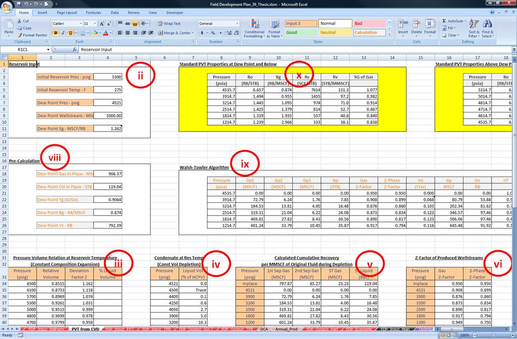
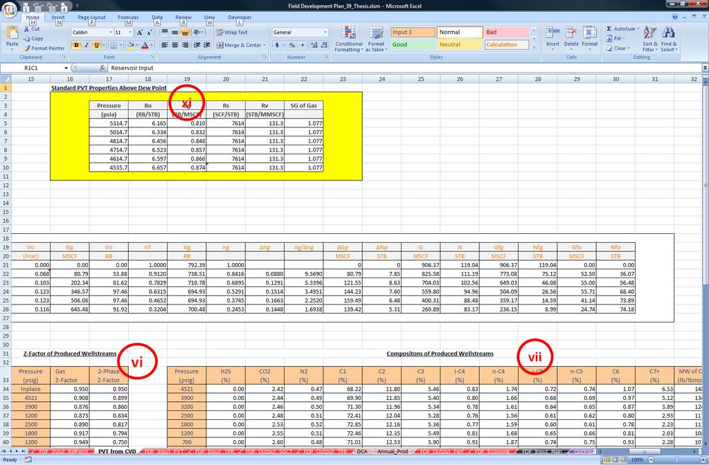
186 171

187 172 b. Simulate standard PVT properties from compositional data i. In PVT_Input_Pres worksheet, input reservoir and surface separators pressure and temperature conditions ii. In PVT_Input_Comp worksheet, input composition (mole fraction) and properties of pure components iii. In PVT_Input_BiCo worksheet, input binary interaction coefficient iv. In PVT_Input_Si worksheet, input volume-translate coefficient data v. In PVT_Output_Prop worksheet, click Calculate Black Oil PVT Properties button vi. In PVT_Output_Envelope worksheet, click Create Phase Envelope button (optional) vii. In FDP_Input_PVT worksheet, click Import from PVT Calculation button

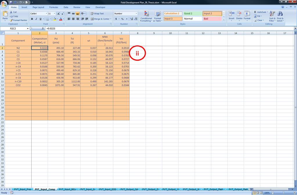
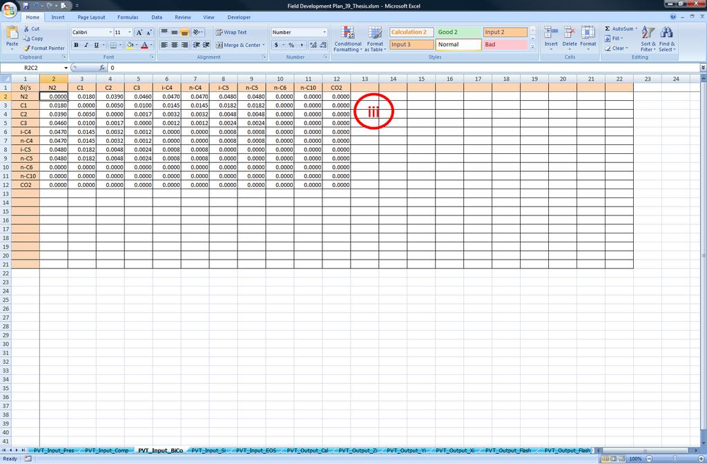
188 173

189 174

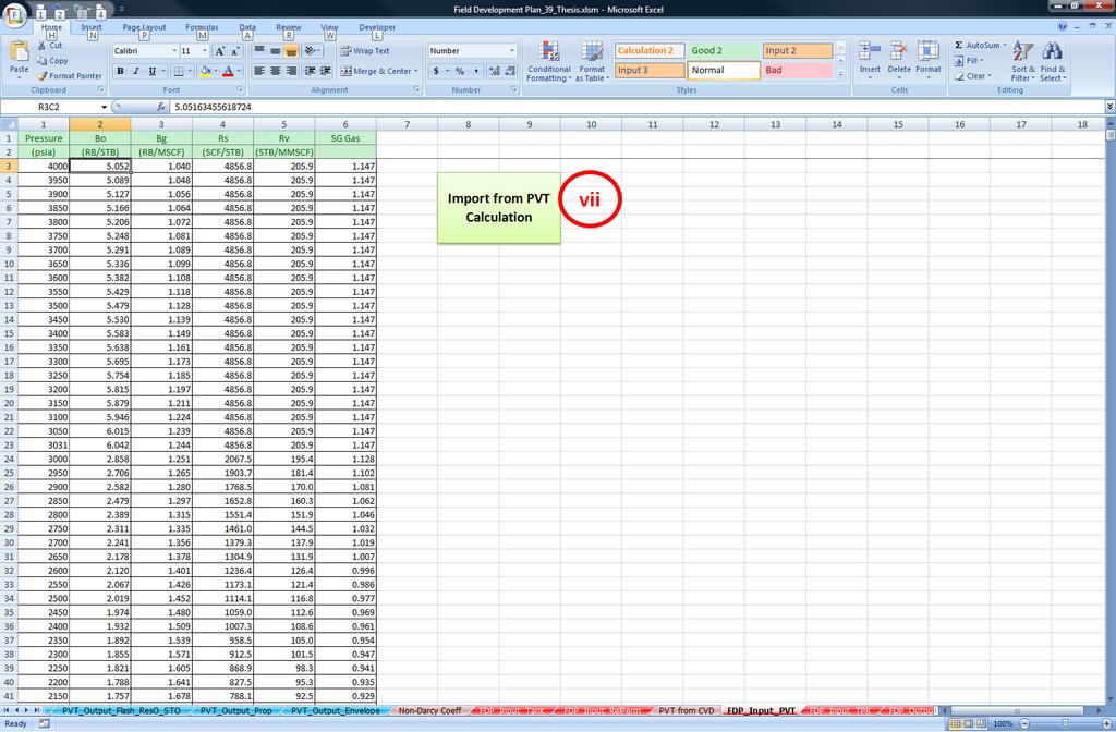
190 175

191 Perform field performance analysis a. Run field performance prediction and economic analysis i. In FDP_Input_Tank worksheet, input reservoir data ii. In FDP_Input_RelPerm worksheet, input relative permeability data iii. In FDP_Input_TPR worksheet, input tubing data iv. In FDP_Economic worksheet, input economic data v. In FDP_Input_Main worksheet, input target recovery factor at end of plateau and total number of wells required for field development vi. Click Run Performance Prediction and Economic Analysis button vii. Obtain economic results from FDP_Economic worksheet viii. Obtain field performance data from FPD_Output_Perf worksheet ix. Obtain reservoir performance data from FDP_Output_SGCT worksheet x. Obtain decline trend analysis data from DCA worksheet xi. Obtain graphical display of flow rates, pressures and cumulative production from QgGp, QoNp, and QwPrPwfPwh worksheets

192 177

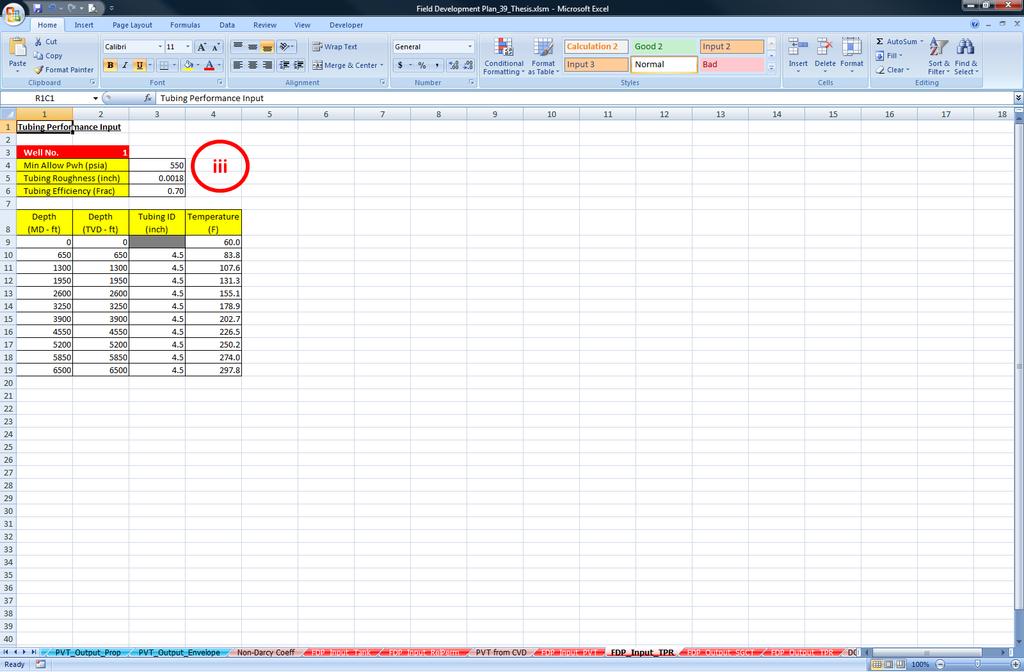
193 178

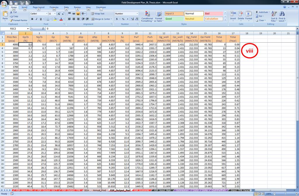
194 179

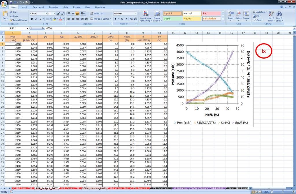
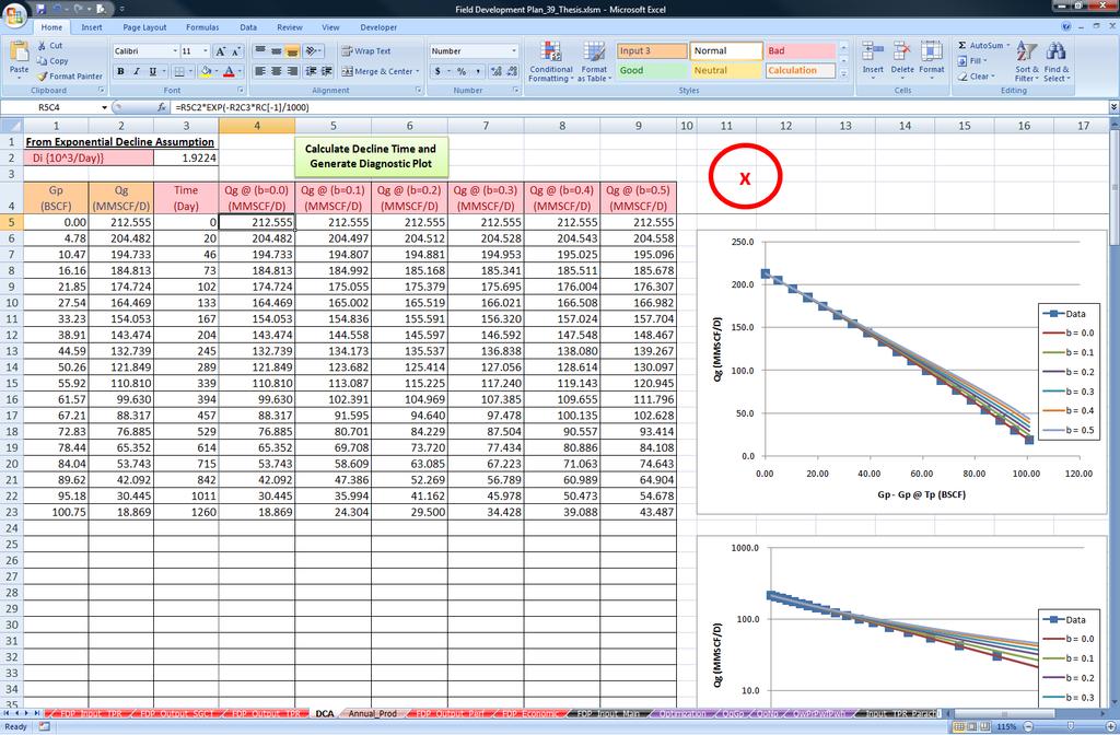
195 180

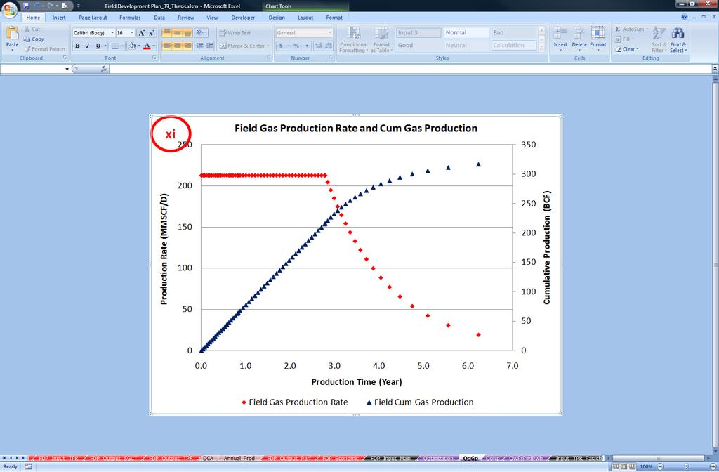
196 181

197 182 b. Run economic analysis from latest field performance data i. In FDP_Economic worksheet, input economic data ii. In FDP_Input_Main worksheet, click Run Economic Analysis from Latest Performance Data button iii. Obtain economic results from FDP_Economic worksheet

198 183

199 Perform field optimization a. Run optimization with new performance prediction and economic analysis i. Repeat 3.-a.-i ) to 3.-a.-iv) ii. In FDP_Input_Main worksheet, input target recovery factor at end of plateau and total number of wells required for field development iii. Click Optimization 1: Run Performance Prediction and Economic Analysis button iv. Obtain field optimization results from Optimization worksheet

200 185 b. Run optimization with new economic analysis only (utilize latest performance prediction data) i. In FDP_Economic worksheet, input economic data ii. In FDP_Input_Main worksheet, click Optimization 2: Run Economic Analysis only button iii. Obtain field optimization results from Optimization worksheet

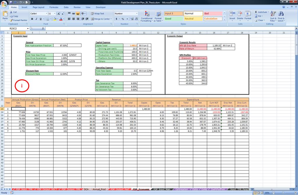
201 186

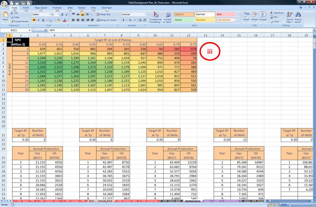
202 187