Unified Corridor Investment Study Step 2 Analysis Results

Transcription

1 Prepared for: Unified Corridor Investment Study Step 2 Analysis Results DRAFT September 2018 Prepared by:

2 This planning study is funded through a Caltrans Sustainable Communities Transportation Planning Grant (FTA 5304) and local voter-approved Measure D funds.

3 Table of Contents INTRODUCTION... 1 Triple Bottom Line Framework... 1 Scenario Analysis... 2 Relationship of the UCS to the Highway 1 EIR SCENARIO ANALYSIS - BASELINE CONDITIONS Safety Safety Baseline Performance Measure Reliability and Efficiency Peak Period Mean Auto Travel Time Peak Period Mean Heavy-Duty Truck Travel Time (SR 1) Peak Period Mean Transit Travel Time Travel Time Reliability Mode Share Person Trips Across North-South Screen Line Peak Period Person Travel Time (Auto Versus Transit Travel Time Comparison) Economic Vitality Level of Public Investment Visitor Tax Revenue Other Economic Benefits Costs Associated with Fatalities and Injuries Environment & Health Automobile and Truck Vehicle Miles Traveled (VMT) Environmentally Sensitive Areas Equitable Access Transit Vehicle Miles Traveled Household Transportation Costs Benefits and Impacts to Transportation Disadvantaged Communities Unified Corridor Investment Study - Draft Step 2 Analysis September 2018 Page i

4 SCENARIO ANALYSIS FORECASTS Safety Injury and Fatal Collisions by Mode Reliability and Efficiency Peak Period Mean Auto Travel Time Peak Period Mean Transit Travel Time Travel Time Reliability Mode Share Person Trips Across North-South Screenlines Economic Vitality Public Investment Visitor Tax Revenue and Other Economic Impacts Cost Associated with Collisions Environment & Health Automobile Vehicle Miles Traveled Environmentally Sensitive Areas Greenhouse Gas and Criteria Pollutants Equitable Access Transit Vehicle Miles Traveled Household Transportation Cost Benefits to Transportation Disadvantaged Communities Transportation Technologies TNC Congestion and Transit Impacts Autonomous Vehicle Adoption Shared Mobility Electric Vehicle Adoption Future Transportation Needs Summary APPENDIX A - PROJECT DESCRIPTIONS AND COST ESTIMATES Unified Corridor Investment Study - Draft Step 2 Analysis September 2018 Page ii

5 APPENDIX B SANTA CRUZ COUNTY TRAVEL DEMAND MODEL OVERVIEW APPENDIX C - BIKE AND WALK MODE SHARE CALCULATIONS APPENDIX D - PERSON TRIPS BY SCREENLINE AND MODE APPENDIX E - PERFORMANCE DASHBOARD List of Tables Table 1: Unified Corridor Investment Study: Goal and Performance Measures... 5 Table 2: Step 1 Scenarios for Analysis... 6 Table 3: Step 2 Scenarios for Analysis... 7 Table 4: Performance Measures and Data Source... 8 Table 5: Corridor Collision History by Segment Table 6: Collision Rates for State Route 1 and Comparison to Similar Facilities ( ) Table 7: Total Study Area Collisions Table 8: Auto Travel Time and Speed for State Route Table 9: Automobile Travel Time and Speed for Soquel Avenue/Drive and Freedom Boulevard Table 10: Heavy Truck Travel Time and Speed for State Route Table 11: Peak Period Transit Travel Times Table 12: SR 1 Travel Time Reliability for Passenger Cars Table 13: Soquel and Freedom Travel Time Reliability for Passenger Cars Table 14: Santa Cruz County Commute Mode Split Table 15: Santa Cruz County All Trip Weekday Mode Split Table 16: Screenline Throughput (4-6 PM Weekday and Daily Auto) Table 17: Transit vs. Auto Travel Time Comparison Table 18: Transient Occupancy Tax Revenue by Jurisdiction, by Fiscal Year Table 19: Estimated Visitor Spending and Visitor Related Local Sales Tax Revenue in Santa Cruz County Unified Corridor Investment Study - Draft Step 2 Analysis September 2018 Page iii

6 Table 20: Estimated Visitor Spending and Visitor Related Local Sales Tax Revenue in Santa Cruz County Table 21: Commercial and Industrial Asking Rents per Square Foot, Inventory, and Vacancy Rates, Third Quarter of Table 22: Apartment Monthly Asking Rents, Third Quarter of Table 23: Average Residential Sales Prices, August 2017 to July 2018 Period Table 24: Taxable Sales by Local Jurisdictions, Table 25: Cost of Collisions Table 26: Project Study Area Baseline Annual Average ( ) Collision Types and Costs Table 27: 2015 Greenhouse Gas and Criteria Pollutants Emissions Table 28: Baseline Transit VMT Table 29: Baseline Household Transportation Costs for an Average Santa Cruz County Household Table 30: Baseline Representative Household Transportation Costs for Santa Cruz County Table 31: Collision Forecasts by Scenario (Fatal, Injury, and Property Damage Only) Table 32: Countywide Mean Auto Speed (mph) Table 33: Countywide Vehicle Hours Traveled (hours) Table 34: Countywide Mean Auto Travel Time (minutes) Table 35: Peak Period Mean Transit Travel Times (minutes) Table 36: Countywide Mode Share by Person Trips Table 37: Screenline Throughput (Person Trips 4-6 PM) Table 38: New Public Investments for Capital Costs- Capital Cost Estimates and Potential Funding Amounts by Project and Scenario Table 39: New Public Investments for Operation and Maintenance Costs- Cost Estimates and Potential Funding Amounts by Project Scenario Table 40: Visitor Related Tax Revenues by Scenario (2015 dollars) Table 41: Summary of Relative Qualitatively-Assessed Economic Benefits Table 42: Costs Associated with the Number of Collisions by Project and Scenario Table 43: Daily Countywide Vehicle Miles Traveled (VMT) Unified Corridor Investment Study - Draft Step 2 Analysis September 2018 Page iv

7 Table 44: Daily Countywide Vehicle Miles Traveled per Capita (VMT/capita) Table 45: UCS Project with New Construction located in Environmentally Sensitive Areas Table 46: 2035 Greenhouse Gas and Criteria Pollutant Emissions Table 47: Annual Transit Vehicle Miles Traveled Scenario Comparison Table 48: Forecasted Average Household Transportation Cost (2018 dollars) Table 49: 2035 Representative Households (2018 dollars) Table 50: Share of Investment Benefit for Transportation Disadvantaged Population List of Figures Figure 1: Triple Bottom Line Framework... 1 Figure 2: Study Area... 4 Figure 3: Countywide Collisions by Severity Figure 4: SWITRS/TIMS Collision Locations- All Collision Types Figure 5: SWITRS/TIMS Bicycle and Pedestrian Collisions Figure 6: Screenline Locations Figure 7: Santa Cruz Hotel Inventory Figure 8: Santa Cruz County Population Density Figure 9: Household Median Income, Figure 10: Educational Attainment High School Degree or Less Figure 11: Educational Attainment, Bachelor's Degree or More Figure 12: Total Employment Density Figure 13: Hotel and Development Projects (Santa Cruz) Figure 14: Hotel and Development Projects (Watsonville) Figure 15: Retail Trade Employment Density Figure 16: Annual cost of Collisions in Santa Cruz County (2016 dollars) Figure 17: Location of Study Area Collisions by Relative Cost Figure 18: VMT for Santa Cruz County Figure 19: Study Area Wetlands and Streams Unified Corridor Investment Study - Draft Step 2 Analysis September 2018 Page v

8 Figure 20: Habitat Corridors Figure 21: Critical Habitat Areas Figure 22: Agriculture Figure 23: Williamson Act Figure 24: Topography Figure 25: Liquefaction Figure 26: Coastal Flooding Figure 27: 100 Year Floodplain Figure 28: Environmental Justice Areas Figure 29: Comparison of Total Collisions in Study Area by Scenario Figure 30: Countywide Mean Auto Speed (mph) Figure 31: Countywide Mode Share by Person Trips Figure 32: Major Existing Activity Nodes Figure 33: Visitor Tax Revenues Figure 34: Costs Associated with Collisions Figure 35: Countywide Vehicle Miles Traveled Figure 36: Environmentally Sensitive Areas Figure 37: Scenario A New Construction and Environmentally Sensitive Area Overlap Figure 38: Scenario B New Construction and Environmentally Sensitive Area Overlap Figure 39: Scenario C New Construction and Environmentally Sensitive Area Overlap Figure 40: Scenario E New Construction and Environmentally Sensitive Area Overlap Figure 41: Annual Transit Vehicle Miles Traveled Scenario Comparison Figure 42: Household Transportation Cost Unified Corridor Investment Study - Draft Step 2 Analysis September 2018 Page vi

9 INTRODUCTION Three parallel routes - Highway 1 1, Soquel Ave/Soquel Dr/Freedom Blvd, and the Santa Cruz Branch Rail Line - link the communities along the Santa Cruz County coast from Davenport through Watsonville. Highway 1 and Soquel/Freedom are heavily traveled, often congested, and emphasize automobile travel. The 2012 acquisition of the rail right-of-way (ROW) provides a parallel transportation facility along this corridor that has unused capacity. A comprehensive evaluation that examines the performance of potential transportation improvements on all three routes when designed to function together as a single unified corridor has not been explicitly analyzed since the purchase of the rail ROW. The UCS builds on prior studies of individual projects or routes. The objective of the Unified Corridor Investment Study (UCS) is to identify multimodal transportation investments that provide the most effective use of Highway 1, Soquel Ave/Soquel Dr/Freedom Blvd, and the Santa Cruz Branch Rail Line to serve the community s transportation needs. The passage of Measure D in November 2016 directed RTC to evaluate future transportation uses of the rail right-of-way (ROW). The Unified Corridor Investment Study will provide an analysis of the options for the rail ROW as required by Measure D, in combination with an evaluation of potential transportation projects on Highway 1 and Soquel Ave/Soquel Dr/Freedom Blvd. Triple Bottom Line Framework The Unified Corridor Study is using a triple bottom line approach as a framework for decision making (Figure 1). This approach evaluates the benefits of various transportation investments in developing a sustainable transportation system that advances triple bottom line goals of economy, environment and social equity. The Santa Cruz County Regional Transportation Commission (RTC) has incorporated triple bottom line sustainability principles in prioritizing projects for funding in the long-range planning process, as well as, programming of funds for project implementation. The legal requirements of Senate Bill 375 to reduce greenhouse gas emissions from transportation and land use, as well as federal requirements in the Moving Ahead for Progress in the 21st Century Act (MAP-21) to improve safety and reduce congestion, and Caltrans Strategic Management Plan target to double pedestrian and transit trips and triple bike trips all necessitate a triple bottom line, performance based approach for making transportation investment decisions. Figure 1: Triple Bottom Line Framework 1 Highway 1 and State Route 1 are used interchangeably in this report. Baseline Conditions Page 1

10 The Unified Corridor Investment Study is evaluating transportation improvements using a performancebased planning and scenario analysis approach consistent with guidance/policy for evaluating future investment decisions of state/federal transportation discretionary funds. This approach increases decision-maker and community understanding by transparently evaluating the benefits and impacts of transportation investments. Best practice standards for a planning level analysis are being utilized in this study to support a quantitative and qualitative analysis for a more informed decision-making process. The approach follows the following steps: Define the project study area (Figure 2) and the forecast year to be Develop the goals of the transportation corridor. Identify performance measures to assess if goals are being advanced (Table 1). Select transportation improvements to evaluate on each of the routes. Combine the projects into scenarios (Table 2). Perform a two-step Scenario Analysis Step 1 - qualitatively evaluate scenarios based on the Step 1 criteria and eliminate scenarios that do not meet criteria (Appendix A) Step 2 quantitatively evaluate remaining scenarios (Table 3) based on the Step 2 performance measures Identify a preferred scenario The project study area includes SR 1 between Davenport and SR 129; Soquel Ave/Soquel Dr/Freedom Blvd from Pacific Ave to Main St; the Santa Cruz Branch Rail Line from Davenport to Pajaro Station outside of Watsonville; and local roadways parallel to the rail right-of-way will be considered as part of the safety analysis. The screenline analysis includes all major arterials that run north-south in the project study area. Goals for the Unified Corridor Study focus on developing a transportation system which seeks to maximize benefits to current and future generations in terms of safety, efficient mobility, environment and health, equity, and economic vitality of the region. The performance measures serve to inform these goals that together promote the triple bottom line framework of economy, environment and healthy communities. Application of the performance measures provides an objective, transparent, data-driven framework for making investment priority decisions. The performance measures are consistent with those described in the 2040 Regional Transportation Plan for Santa Cruz County and were selected based on public input and availability of data that is required for the analysis. Scenario Analysis Development of the scenarios is based on establishing groups of complimentary transportation improvements that are multimodal and reflect community expectations that the study corridor will provide a range of transportation options by The transportation improvements to be evaluated in the scenarios are broken out by each route - Highway 1, Soquel Ave/Soquel Dr/ Freedom Blvd, and the rail ROW. More detailed descriptions for each of the projects can be found in Appendix A. The three auxiliary lane projects funded by Measure D (Soquel to 41 st, Bay/Porter to Park, and Park to State Park) are assumed to be constructed in every scenario. Step 1 of the Unified Corridor Study qualitatively evaluated six scenarios for the study corridor (Table 2). The Step 1 analysis determined two of the scenarios would not likely be feasible and/or were not congruent with community input. These two scenarios were dropped from further consideration. In addition, two of the remaining four scenarios were slightly modified to be more modally balanced. Results of Step 1 can be found in Appendix A. Input has been encouraged throughout development of the Unified Corridor Investment Study. Participation from diverse sets of transportation interests including members of the public, community organizations, stakeholders, and partner agencies have been solicited at key milestones to provide input in this study. The Step 2 scenario analysis quantitatively evaluates the remaining four scenarios (Table 3). Given the quantitative nature of the Step 2 analysis, evaluation methods were selected/developed considering the Baseline Conditions Page 2

11 available data required for the analysis tools, the various types of projects, and the output needed to inform the performance measures. Table 4 provides a summary of the data sources and analysis methods used to quantify both the baseline existing conditions and the future projections. Step 2 requires an evaluation of the baseline conditions for each of the performance measures in order to compare against future scenarios and a no-build. Establishment of an accurate baseline condition is critical for determining the change in benefit anticipated from a given scenario. The initial sections of this report will describe in greater detail the baseline data and analysis methods listed in Table 4. A subsequent section will focus on the forecasting methodology and relative performance of the four scenarios with project groupings and the no-build under future year conditions. Completion of the Step 2 analysis is intended to result in a preferred scenario or group of projects recommended for implementation. Baseline Conditions Page 3

12 Figure 2: Study Area Baseline Conditions Page 4

13 Table 1 lists the project goals and the respective performance measures that inform each. Table 1: Unified Corridor Investment Study: Goal and Performance Measures Baseline Conditions Page 5

14 Table 2: Step 1 Scenarios for Analysis Unified Corridor Investment Study - Step 1 Scenarios for Analysis (RTC Approved - June 15, 2017) Highway 1 Projects buses on shoulders high occupancy vehicle lanes (HOV) and increased transit frequency auxiliary lanes to extend merging distance IN ADDITION TO MEASURE D metering of on-ramps additional lanes on bridge over San Lorenzo River Mission St intersection improvements rail transit on Hwy 1 between Santa Cruz and Watsonville self driving cars Soquel Avenue/Drive and Freedom Blvd bus rapid transit lite (faster boarding, transit signal priority and queue jumps) dedicated lane for bus rapid transit and bikes parking moved from Soquel Avenue/Drive to improve bike and transit options increased frequency of transit with express services buffered/protected bike lanes intersection improvements for auto intersection improvements for bikes/pedestrians Rail Corridor multiuse trail (bike and pedestrian) bike trail separate from pedestrian trail local rail transit with interregional connections bus rapid transit freight service on rail Overall Project Area/Connections between Routes improved bike/pedestrian facilities throughout urban area closing gaps in network additional transit connections bike share, bike amenities, transit amenities, park and ride lots multimodal transportation hubs Transportation Demand and System Management employers and residences - incentive programs education and enforcement - electric vehicle, motorist safety, and bike safety Scenario A Scenario B Scenario C Scenario D Scenario E Scenario F No Build These projects will be evaluated in all scenarios. These projects will be evaluated in all scenarios. bus transit rail transit auto bike/ped rail freight Baseline Conditions Page 6

15 Table 3: Step 2 Scenarios for Analysis Unified Corridor Investment Study - Step 2 Scenarios for Analysis (Approved by RTC on December 7, 2017 *) Highway 1 Projects buses on shoulders high occupancy vehicle lanes (HOV) and increased transit frequency auxiliary lanes to extend merging distance IN ADDITION TO MEASURE D metering of on-ramps additional lanes on bridge over San Lorenzo River Mission St intersection improvements Soquel Avenue/Drive and Freedom Blvd bus rapid transit lite (faster boarding, transit signal priority and queue jumps) increased frequency of transit with express services buffered/protected bike lanes intersection improvements for auto intersection improvements for bikes/pedestrians Rail Corridor bike and pedestrian trail local rail transit with interregional connections bus rapid transit freight service on rail Overall Project Area/Connections between Routes improved bike/pedestrian facilities throughout urban area closing gaps in network additional transit connections bike share, bike amenities, transit amenities, park and ride lots multimodal transportation hubs automated vehicles/connected vehicles Transportation Demand and System Management employers and residences - incentive programs education and enforcement - electric vehicle, motorist safety, and bike safety *Scenarios D and F were eliminated from evaluation in Step 2 Scenario A Scenario B Scenario C Scenario E No Build Only Watsonville These projects will be evaluated in all scenarios. These projects will be evaluated in all scenarios. bus transit rail transit auto bike/ped rail freight Baseline Conditions Page 7

16 Table 4: Performance Measures and Data Source Performance Measure Baseline Data Source 2035 Forecasting Methodology Injury and fatal collisions by mode Peak period mean automobile travel time CHP SWITRS dataset, Caltrans TASAS NPMRDS Auto and Truck Speed Data (SR 1) StreetLight Speed Data (Soquel and Freedom) Federal Highway Administrations CMF Clearinghouse Highway Safety Manual Part C Predictive Methods SCC Travel Demand Model HCM 6 th Edition Peak period mean transit travel time Santa Cruz Metro Schedule Information SCC Travel Demand Model Peak period person travel time 2 Peak period travel time reliability Google Maps - origin to destination times based on time of day Santa Cruz Metro Schedule Information NPMRDS Speed Data (SR 1) StreetLight Speed Data (Soquel and Freedom) Federal National Performance Measurement Rule Guidance SCC Travel Demand Model Qualitative forecast based on project increases/decreases in congestion Mode share California Household Travel Survey (CHTS) NCHRP 552 (ped/bike) - modified for Santa Cruz County American Community Survey SCC Travel Demand Model Person trips across N-S screen line 2016 Motor Vehicle, Bicycle and Pedestrian Traffic Counts collected by RTC NCHRP 552 (ped/bike) - modified for Santa Cruz County 2 This measure is added to provide a comparison of auto and transit travel times between specific origins and destinations. Baseline Conditions Page 8

17 Performance Measure Baseline Data Source 2035 Forecasting Methodology Level of public investment Visitor tax revenue Cost associated with fatalities and injuries Transit Ridership from 2012 On Board Transit Study No baseline data needed for this measure Sales and Transient Occupancy Tax data from Board of Equalization and Runyan Associates report California Travel Impacts by County, Caltrans Economics Analysis Branch Vehicle Operation Cost Parameters; National Highway Traffic Safety Administration SCC Travel Demand Model Project costs estimated by Kimley-Horn, updated from previous studies, or based on cost estimates in the 2040 RTP; Potential funding sources based on 2040 RTP and updated if new information is available and on professional experience Based on estimated changes in visitor volumes and relative impacts of scenarios on travel time, vehicle miles traveled and transit and bicycle ridership Based on results from "Number of Injury and Fatal collisions" performance measure. Costs per collision by severity will remain in 2016 dollars Automobile vehicle miles traveled Caltrans Highway Performance Monitoring System (HPMS) SCC Travel Demand Model Environmentally sensitive areas Multiple sources including USFW, Caltrans, UC Davis, CA Dept of Conservation, FEMA, Monterey Bay Sanctuary Foundation, and the US Geological Survey GIS analysis of length of overlap of locations with new construction and environmentally sensitive areas Criteria pollutants Greenhouse gas emissions VMT from Highway Performance Monitoring System (HPMS) CA Air Resource Board 2014EMFAC model SCC Travel Demand Model VMT by speed VMT from Highway Performance Monitoring System (HPMS) CA Air Resource Board 2014EMFAC model SCCRTC Travel Demand Model VMT by speed SCC Travel Demand Model VMT CA Air Resources Board 2014EMFAC model SCC Travel Demand Model - VMT by speed SCC Travel Demand Model VMT CA Air Resources Board 2014EMFAC model SCC Travel Demand Model - VMT by speed Transit vehicle miles traveled National Transit Database SCC Travel Demand Model Baseline Conditions Page 9

18 Performance Measure Baseline Data Source 2035 Forecasting Methodology Caltrans Economics Analysis Branch Vehicle Operation Cost Parameters AAA 2017 Your Driving Costs Household transportation costs Benefits and burdens to environmental justice communities EMFAC Fuel Economy for Santa Cruz County Transit Revenue Census Data SCCRTC 2040 RTP - Definition of Transportation Disadvantaged Communities U.S Census Bureau data AB1550/California Housing and Community Development Based on mode share results; CA Household Travel Survey data on typical travel distances by mode GIS analysis to determine projects that are in areas with transportation disadvantaged communities SCC Travel Demand Model Note: NPMRDS - National Performance Management Research Data Set SCC - Santa Cruz County HCM - Highway Capacity Manual SWITRS - Statewide Integrated Traffic Records System CHP - California Highway Patrol Metro - Santa Cruz Metropolitan Transit District NCHRP - National Cooperative Highway Research Program AAA - Automobile Association of America TASAS - Traffic Accident Surveillance and Analysis System CMF - Collision Modification Factor USFW- United States Fish and Wildlife Service FEMA- Federal Emergency Management Agency Baseline Conditions Page 10

19 Relationship of the UCS to the Highway 1 EIR The purpose of the Santa Cruz Route 1 Tier 1 and Tier 2 Environmental Impact Report (EIR) is to disclose the environmental effects of implementing near term corridor improvements on Highway 1 that are a high priority for Caltrans and the SCCRTC. The EIR is being prepared in support of a Project Approval document for the Soquel to 41st Ave Auxiliary Lanes Project (aka Tier 2 project). This Tier 2 project will proceed into the design phase and could start construction in This EIR provides analysis at a level of detail necessary for project approval of the Tier 2 project, and discloses the potential environmental effects of future projects along the SR 1 corridor to reduce congestion and promote alternative modes of transportation (Tier I HOV/TSM Alternatives). Any action to pursue the Tier 1 improvements in the future will require more detailed analysis as part of a subsequent decision process. The purpose of the UCS is to analyze the parallel transportation corridors together and to provide information that would establish future priorities for corridor investments beyond the Tier 2 Auxiliary lanes project. The UCS evaluation considers a broad range of scenarios along the parallel network comprised of Highway 1, local arterials and the railroad. Any recommendations on a future investment strategy would then be subject to further development, evaluation and a subsequent approval process that would also require environmental review. While a variety of improvements to Highway 1 are considered in both documents (EIR and UCS), these documents each support different decisions for implementation across variable timeframes in an overall transportation investment strategy. To satisfy their unique objectives, the Traffic Studies performed for each document also differ. The performance measures in the HOV/TSM (EIR) analysis are based on a refined and detailed analysis using a number of traffic modeling tools for Highway 1, whereas the UCS used a countywide travel demand model to look at much of the roadway network throughout the county including Highway 1. The Tier 2 improvements are presented in the EIR for near-term implementation. The information presented for Tier 1 improvements and the UCS both support future decisions about the type of investments to follow. SCENARIO ANALYSIS - BASELINE CONDITIONS Establishing an accurate baseline allows a determination of how much benefit each scenario would provide relative to existing conditions. Baseline conditions were established for each performance measure listed in Table 3, with the exception of the level of public investment measure for which no baseline is needed. A description of each performance measure s baseline derivation is provided in the subsequent sections. The baseline conditions for performance measures typically reflect 2015 conditions, unless otherwise noted. Safety Safety is a critical measure for community well-being, quality of life, and particularly in the case of active transportation facilities, accessibility. The goal of Safer Transportation for All Modes is measured by assessing the number of fatal and injury collisions by mode for baseline conditions compared to 2035 forecasts. Baseline data for the study area is acquired using the five most recent years ( ) of final collision data from the Statewide Integrated Traffic Records System (SWITRS), SafeTrec s Traffic Injury Mapping System (TIMS) and Caltrans Traffic Accident Surveillance and Reporting System (TASAS). More recent collision data is considered provisional and therefore is not used in this analysis. Each of these datasets provide unique information that serves to inform a safety evaluation. The SWITRS dataset provides the most comprehensive record of collision activity countywide as it tracks fatalities, injuries and property damage only collisions. The TIMS dataset is a geo-coded extract of SWITRS data focused on injury and fatal collisions only. TIMS collision records are precisely geo-located and can therefore be reliably Baseline Conditions Page 11

20 mapped to roadways. TASAS is an aggregated set of collision information available only for state highways. TASAS data provides collision rates (number of collisions/vehicle miles traveled) for roadway corridor segments which can be compared against other similar corridors within California. SWITRS has 16,980 collision records spanning from 2011 through 2015 in Santa Cruz County. Figure 3 shows the annual trend of countywide collisions between 2011 and The countywide collision total has trended slightly upward since 2013, including an increase in collision severity. There is an average of 3,396 collisions per year countywide. The number of collisions for this 5-year time period in each of the jurisdictions are provided below. 2,639 City of Santa Cruz 617 City of Capitola 2,619 City of Watsonville 652 City of Scotts Valley 10,453 Unincorporated Table 5 provides a detailed breakdown of the collisions in the Unified Corridor Study area by roadway segment and mode. For this metric, the study area also includes roadways parallel to the rail right-of-way that would likely see changes in their use once a bicycle and pedestrian trail is established along the rail right of way. Between 2011 and 2015, there were 1,989 injury and 17 fatal collisions recorded along study area roadways 3. Six of the fatal collisions involved bicyclists or pedestrians (three on Soquel Ave/Dr, two on SR 1 along the north coast and one on Mission St.) Eight of the fatal collisions not involving bicyclists or pedestrians occurred on SR 1 between Highway 129 and SR 17. Motor vehicle collisions involving a bicycle or pedestrian injury or fatality account for 22% of the total injury and fatal collisions in the UCS study area collisions involved a pedestrian and 304 collisions involved a bicycle. Collisions that did not result in an injury or fatality (property damage only collisions) have not been delineated by roadway segments for the project study area as these collisions do not consistently have their locations specified. Figure 4 maps the location of injury and fatal collisions along State Route 1 (SR 1), Soquel Avenue/Soquel Drive/Freedom Boulevard and roadways that serve as parallels to the Santa Cruz Branch Rail Line. Bicyclists and pedestrians could relocate from these parallel roadways to the trail on the rail right-of-way and thus, are being evaluated for assessing bicycle and pedestrian collisions in future potential scenarios. Figure 5 shows just the bicycle and pedestrian collisions in the project study area. Caltrans TASAS analytics have indicated several segments, interchanges and intersections of SR 1 that after normalizing for demand usage, are experiencing more collision activity than would be expected based on the performance of similar facilities elsewhere in the state. SR 1 in the project study area for the five-year period from 2011 to 2015 had a collision rate of 0.96 collisions per million vehicle miles traveled (MVMT). For like facilities elsewhere in the State, the expected collision rate is Table 6 lists the segments of SR 1 in the study area and their collision rate performance relative to expected. Segments of SR 1 with more collisions than expected based on peer facility performance are most common along the arterial section (Mission Street) through the City of Santa Cruz and the freeway section near 41 st Ave in Capitola. 3 Four of the collisions involve both bicycles and pedestrians, two of which reported both pedestrian and bicycle injuries and are therefore counted twice in Table 5. The collision total of 2006 is therefore two less than the total number of collisions in Table 5. Baseline Conditions Page 12

21 Figure 3: Countywide Collisions by Severity Baseline Conditions Page 13

22 Injury Fatal Injury Fatal Injury Fatal Table 5: Corridor Collision History by Segment Segment Vehicle Bicycle Pedestrian SR 1 SR 129 SR 152/Main Street SR 152/Main San Andreas Road San Andreas Road Freedom Boulevard 31 Freedom Boulevard State Park Drive State Park Drive Bay Avenue Bay Avenue Soquel Drive Soquel Drive Morrissey Boulevard Morrissey Boulevard SR SR 17 Bay Drive Bay Drive Shaffer Road Shaffer Road Dimeo Lane 15 3 Dimeo Lane Marine View Avenue Soquel Drive Freedom Boulevard State Park Drive State Park Drive Porter Street Porter Street 41st Avenue st Avenue Paul Sweet Road Paul Sweet Road Pacific Avenue Freedom Boulevard SR 152/Main Street Buena Vista Drive Buena Vista Drive White Road White Road SR SR 129 Walker Street Lee Road 24 Beach Street / San Andreas Road Corridor Walker Street SR SR 1 San Andreas Road 6 Baseline Conditions Page 14

23 Injury Fatal Injury Fatal Injury Fatal Segment Vehicle Bicycle Pedestrian Beach Street Buena Vista Drive Buena Vista Drive Seascape Boulevard 11 1 Sumner Avenue Via Novella Seascape Boulevard Seascape Boulevard Rio Del Mar Boulevard 2 McGregor Drive / Park Avenue / Portola Drive / San Lorenzo Boulevard Corridor Searidge Drive Park Avenue McGregor Drive Bay Street Park Avenue Capitola Avenue Monterey Avenue Soquel Wharf Road Soquel Wharf Road 7 th Avenue Cliff Drive Eaton Street th Avenue Cliff Drive Capitola Road / Soquel Wharf Road Corridor Stockton Street 41 st Avenue st Avenue 7 th Avenue Brommer Street 41 st Avenue 17 th Avenue Nova Drive Portola Avenue 41 st Avenue 1 1 Bay Street Beach Street California Street Delaware Avenue / Shaffer Road Corridor Bay Street Shaffer Road Total 1 1, Motor vehicle collisions involving bicycles or pedestrians are listed under bicycle or pedestrian collisions. Two of the collisions reported both pedestrian and bicycle injuries and are therefore included under both bicycle injury and pedestrian injury collisions in Table 5. The total of 2,008 in this table is therefore two more than the 2,006 total number of collisions in for the project study area. Baseline Conditions Page 15

24 Figure 4: SWITRS/TIMS Collision Locations- All Collision Types Baseline Conditions Page 16

25 Figure 5: SWITRS/TIMS Bicycle and Pedestrian Collisions Baseline Conditions Page 17

26 Table 6: Collision Rates for State Route 1 and Comparison to Similar Facilities ( ) Segment Observed Rate 1 Expected Rate 2 Difference SR 129 NB Off Ramp SR 129 NB On Ramp SR 129 NB On Ramp Harkins Slough Rd Harkins Slough Rd Airport Blvd NB On Ramp Airport Blvd NB On Ramp Buena Vista Dr NB Off Ramp Buena Vista Dr NB Off Ramp Buena Vista Dr NB On Ramp Buena Vista Dr NB On Ramp Mar Monte Ave NB Off Ramp Mar Monte Ave NB Off Ramp Mar Monte Ave NB On Ramp Mar Monte Ave NB On Ramp Larkin Valley Rd Larkin Valley Rd Park Ave Park Ave Bay Ave Bay Ave 41st Ave NB Off Ramp st Ave NB Off Ramp 41st Ave NB On Ramp st Ave NB On Ramp Soquel Dr NB Off Ramp Soquel Dr NB Off Ramp Soquel Dr NB On Ramp Soquel Dr NB On Ramp Emeline Ave NB Off Ramp Emeline Ave NB Off Ramp River St River St Mission St Mission St Locust St Locust St Walnut Ave Walnut Ave Laurel St Laurel St Bay St Bay St Almar Ave Almar Ave Swift St Swift St Santa Cruz City Limit Santa Cruz City Limit 400' east of Coast Rd ' east of Coast Rd 400' west of Coast Rd ' west of Coast Rd 2101 Coast Rd Coast Rd Dimeo Ln Dimeo Ln Four Mile Beach Parking Four Mile Beach Parking Rodoni Farms Rodoni Farms Scaroni Road Scaroni Road Marine View Ave Collisions per million vehicle miles traveled 2 Collisions per million vehicle miles traveled, expected rates from TASAS Table B Baseline Conditions Page 18

27 Property Damage Only * Injury Fatal Injury Fatal Injury Fatal Safety Baseline Performance Measure The baseline for injury and fatal collisions performance measure is presented below in Table 7 is a yearly average of the number of collisions in the study area. These values will be used as a way to compare the safety benefits of the various projects and scenarios compared to the existing baseline. Table 7: Total Study Area Collisions Vehicle Collisions Bicycle Collisions Pedestrian Collisions One Year Average Baseline Yearly Performance Measure *Property Damage Only Collisions for the study area were estimated by applying the ratio of countywide property damage only to injury and fatal (1.77) to the study area injury and fatal. It is assumed here that there are no property damage only bicycle and pedestrian collisions. Reliability and Efficiency A transportation system that meets the needs of its users provides options for how to travel in a timely and reliable manner. The goal of Reliable and efficient transportation choices that serve the most people and facilitate the transport of goods will be evaluated by assessing the following performance measures: peak period mean auto and transit travel time and travel time reliability, mode share and person trips across a screenline for baseline conditions compared to 2035 forecasts. A comparison of auto travel time and transit travel time evaluates the difference in travel time between automobile and transit person trips for select origin -destination pairs within Santa Cruz County and serves as a peak period person travel time performance measure. Peak period person travel time is also used to assess the UCS reliability and efficiency goal for baseline conditions compared to 2035 forecasts. Peak Period Mean Auto Travel Time Auto travel time is an indicator of the distance traveled, speeds, and congestion experienced by individuals traveling by automobile. Peak periods provide information about times when travel demand is the highest. The automobile peak period travel time is measured using a combination of data available from the Federal Highway Administration, Caltrans and vendors of cell data. For SR 1 traffic speed, estimates were acquired using the National Performance Measurement Research Data Set (NPMRDS) from the Federal Highway Administration. For Soquel/Freedom, cellular data from StreetLight is used to determine travel time. Travel times and speeds for SR 1 Soquel Ave/Dr and Freedom Blvd are shown in Tables 8 and 9, respectively. The travel time data from NPMRDS that is used for SR 1 is from February 1, 2017 to September 30, SR 1 peak traffic hours, as defined by the NPMRDS, are 7:40 AM to 8:40 AM in the morning and 4:40 PM to 5:40 PM in the afternoon. The travel time data for Soquel Ave/Dr and Freedom Blvd from Streetlight is collected from January 1, 2017 to December 31, StreetLight defines the morning peak period as 6:00 AM to 9:00 AM and the afternoon peak period as 4:00 PM to 7:00 PM. Consistent with the Federal Performance Measurement Rule, congestion is determined based on Baseline Conditions Page 19

28 average peak period speed at or below 60% of free flow speed. Free flow speed is the average speed during low volume conditions where drivers are free to travel at their desired speed. It is determined from the average speed from midnight to 3 AM. Free flow speed is adjusted to the peak period speed if the data shows free flow slower than peak period speed. Congested segments during peak periods are indicated with highlighting. The travel time index (TTI) is a ratio of the peak period travel time to the free flow travel time and can be used to compare the performance of the various roadway segments. The TTI is calculated for both the AM and PM peak periods. A TTI of 1.0 is where the peak period travel time is equal to the free flow travel time. A TTI of 1.7 or greater (shown in red) indicates areas with more significant congestion. The segments of SR 1 that have the most significant congestion are from SR 17 to State Park Drive in the SB direction during the PM peak period and from San Andreas to Bay Ave in the NB direction during the AM peak period. The travel time can be up to six times longer than free flow conditions with speeds as low as 10 mph. SR 1 has mostly directional traffic congestion during the peak periods. The AM peak experiences congestion in the northbound direction between San Andreas Rd and Bay Ave/Porter Rd. Congestion in the PM peak occurs primarily in the southbound direction between SR 17 and State Park Drive. Traffic on Mission St is typically congested in both directions during both AM and PM peak periods. Highway traffic in vicinity of Watsonville is generally free of traffic at all times of the day. Southbound traffic south of Freedom Boulevard is generally free of congestion at all times of the day. Peak Period Mean Heavy-Duty Truck Travel Time (SR 1) Truck travel times can differ from auto travel times and can impact the time it takes to distribute goods and services. Heavy-duty truck travel time is measured using NPMRDS data during the same time periods as the auto travel time and results are shown in Table 10. Heavy-duty truck speeds are typically lower than passenger vehicle speeds due to posted highway speed limits for heavy-duty trucks that are set lower than passenger vehicles and the greater gross vehicle weight affects their operational speed particularly if steep grades are present. Southbound traffic south of Freedom Boulevard is generally free of congestion at all times of the day. SR 1 truck traffic between Soquel and State Park Drive experiences mostly directional congestion during the peak periods northbound in the AM and southbound in the PM. Baseline Conditions Page 20

29 Table 8: Auto Travel Time and Speed for State Route 1 Northbound Segment Length (mi) AM Average Speed (mph) 1,2 PM Average Speed (mph) 1,2 Free Flow Speed (mph) 3 AM Average Travel Time (min) 2 PM Average Travel Time (min) 2 AM Travel Time Index 2 PM Travel Time Index 2 SR 129 SR 152/Main Street :55 1: SR 152/Main San Andreas Rd :25 4: San Andreas Rd Freedom Blvd :08 0: Freedom Blvd State Park Drive :38 2: State Park Drive Bay Avenue :44 2: Bay Avenue Soquel Drive :47 1: Soquel Drive SR :31 2: SR 17 Shaffer Road :32 10: Shaffer Road Dimeo Lane :50 2: Summary Northbound SR 129 San Andreas Road :20 6: San Andreas Road SR :50 9: SR 17 Dimeo Lane :22 12: Southbound Dimeo Lane Shaffer Road :52 2: Shaffer Road SR :06 11: SR 17 Soquel Drive :57 5: Soquel Drive Bay Avenue :55 10: Bay Avenue State Park Drive :48 7: State Park Drive Freedom Blvd :09 2: Freedom Blvd San Andreas Rd :59 1: San Andreas Rd SR 152/Main Street :25 4: SR 152/Main Street SR :05 2: Summary Southbound Dimeo Lane SR :57 14: SR 17 San Andreas Road :47 27:21: San Andreas Road SR :30 6: Speed data from NPMRDS. 2 AM peak period is 7:40 to 8:40 AM. PM peak period is 4:40 to 5:40 PM. 3 Data not available north of Dimeo Lane Baseline Conditions Page 21

30 This page left intentionally blank. Baseline Conditions Page 22

31 Soquel Segment Table 9: Automobile Travel Time and Speed for Soquel Avenue/Drive and Freedom Boulevard Length (mi) AM Average Speed (mph) 2 PM Average Speed (mph) 3 Free Flow * Speed AM Average Travel Time (min) 1,2 PM Average Travel Time (min) 1,3 AM Travel Time Index 2 Ocean Street Paul Sweet Road :17 9: Paul Sweet Road 41st Avenue :29 7: st Avenue Porter Street :37 4: Porter Street State Park Drive :16 9: State Park Drive Freedom :32 7: Freedom SR 1 White Road :26 6: White Road Buena Vista Drive :58 6: Buena Vista Drive SR 152/Main Street :58 10: Speed data from StreetLight archives are reported in whole numbers 2 AM Peak: 6AM 9 AM 3 PM Peak: 4PM 7PM * Some sections do not have free flow speeds, used the adjacent section to determine FFS Note- Buena Vista to White has a FFS of 5 mph, this cannot be accurate so used SR 1 to White Road as FFS PM Travel Time Index 3 Baseline Conditions Page 23

32 Table 10: Heavy Truck Travel Time and Speed for State Route 1 Segment Length (mi) AM Average Speed (mph) 1 PM Average Speed (mph) 2 Free Flow Speed (mph) AM Average Travel Time (min) 1 PM Average Travel Time (min) 2 AM Travel Time Index 1 PM Travel Time Index 2 Northbound SR 129 SR 152/Main Street :01 2: SR 152/Main Street San Andreas Road :18 6: San Andreas Road Freedom Boulevard :13 1: Freedom Boulevard State Park Drive :43 3: State Park Drive Bay Ave / Porter Street :47 3: Bay Ave / Porter Street Soquel Drive :52 2: Soquel Drive SR :50 3: SR 17 Shaffer Road :31 11: Shaffer Road Dimeo Lane :49 4: Southbound Dimeo Lane Shaffer Road :40 3: Shaffer Road SR :43 14: SR 17 Soquel Drive :45 7: Soquel Drive Bay Ave / Porter Street :40 8: Bay Ave / Porter Street State Park Drive :00 7: State Park Drive Freedom Boulevard :07 3: Freedom Boulevard San Andreas Road :28 1: San Andreas Road SR 152/Main Street :40 5: SR 152/Main Street SR :09 2: AM Peak: 6AM 9 AM 2 PM Peak: 4PM 7PM Baseline Conditions Page 24

33 Peak Period Mean Transit Travel Time A mean transit travel time performance measure provides a mechanism for assessing whether transit travel times will improve with project implementation. Due to lack of data on real time transit travel times, the mean transit travel time is evaluated by reviewing 2018 published transit schedules. Transit schedules are based on the time that is typically needed for the bus to reach the various locations and thus is representative of baseline conditions. Transit routes serving the SR 1 and Soquel Drive corridors are segmented per their published schedule time points. Travel time is analyzed for Santa Cruz Metro routes 55, 66, 68, 69W, 69A, 71, and 91X. Table 11 shows the AM peak period travel time, PM peak period travel time, first mile, last mile, and wait time. Baseline Conditions Page 25

34 Table 11: Peak Period Transit Travel Times Peak Period Mean Transit Travel Times (Minutes) Route Location Direction AM Travel Time PM Travel Time AM Round Trip Time PM Round Trip Time First Mile 2 Last Mile 2 Wait Time Between Capitola Mall and Via Pacifica Between Pacific Station and Capitola Mall Loop EB WB Between Pacific Station and Capitola Mall EB WB W Between Santa Cruz and Watsonville EB WB A Between Santa Cruz and Watsonville EB WB Between Santa Cruz and Watsonville EB WB X Between Santa Cruz and Watsonville EB WB Wait time calculated as the square root of peak headway 2 Assumes average of ¼ mile walk between bus stop and origin destination and walking speed of 4.5 feet per second Baseline Conditions Page 26

35 The PM peak-hour travel times were slightly longer for many of the segments, attributable to higher levels of congestion during this time of day, with two exceptions. On Route 69A, the inbound travel time between the Nielson stop at Watsonville Hospital and the Capitola Mall bus stop is more than 10 minutes higher during the AM peak-hour than during the PM travel times, likely due to high congestion around 8 AM on SR 1 in the northbound direction. The inbound travel time for Route 91X between the Green Valley & Main and Cabrillo College is more than 15 minutes higher during the AM peak-hour, again attributable to higher levels of congestion around the school in the AM peak-hour. Buses traveling along SR 1 between Watsonville and Aptos are delayed the most by peak period directional congestion. Soquel Drive is most affected by congestion for eastbound traffic during the PM peak period, nearly doubling travel times between Dominican Hospital and 41 st Avenue. Areas in Downtown Santa Cruz are also impacted by PM peak congestion. An overall transit travel time performance measure can best be summarized by a comparison of transit trip s travel times to auto travel times between specific locations. The actual person trip travel time comparison is described in the travel time by origin-destination pair performance measure. Travel Time Reliability An important transportation performance metric advocated at both the federal and state levels is travel time reliability which is a measure of the variability of the travel time from day to day during the same time period. How predictable travel time is can be critical for commuters, goods movement, and transit provision. The larger the variability in travel time, the more unreliable the trip time becomes. The primary causes of unreliable travel times are collisions and an imbalance between demand and capacity that causes congestion. Although when congestion is recurring, a congested system can often become more reliable as the travel time is more predictably longer than free flow conditions. The federal National Highway System Performance Measure Rule specifically mandates State s and Metropolitan Planning Organizations to measure travel time reliability on the National Highway System. Given that SR 1 within the study area is federally designated as part of the National Highway System (NHS), travel time reliability is assessed using the Federal Highway Administration s NPMRDS data and use guidance described in the National Performance Measurement Rule. Reliability is measured for each roadway segment that is analyzed for travel time in both the AM and PM. This includes the Study Area portion of SR 1, and Soquel Avenue/Drive and Freedom Blvd. Travel time reliability is reported as the difference (buffer time) and ratio (buffer time index) of the median 50 th percentile travel time to the 80 th percentile travel time. The 80th percentile travel time is defined as the time when 80% of the trips are shorter than this time. The travel time data used for assessing travel time reliability on SR 1 is from the same time period (from February 1, 2017 to September 30, 2017) that is used in the travel time analysis. The time from 7:40 to 8:40 AM is considered the AM peak period and 4:40 to 5:40 PM is considered the PM peak period. StreetLight Data is used for analyzing travel time reliability on Soquel Ave/Soquel Dr/Freedom Blvd using the same metrics as described for SR 1. Travel time data on Soquel and Freedom from January 1, 2017 to December 31, 2017 is used for this analysis. The time from 6:00 to 9:00 AM is considered the AM peak period and 4:00 to 7:00 PM is considered the PM peak period. The results for SR 1, Soquel Drive and Freedom Boulevard are shown in Table 12 and Table 13. According to the Federal Highway Administration, a Buffer Time Index less than 25% is considered reliable, a buffer time index between 25% and 50% is mostly reliable, and a buffer time index greater than 50% is considered unreliable. In Table 12 and Table 13 green denotes reliable conditions, yellow denotes moderately reliable conditions, and red denotes unreliable conditions. Baseline Conditions Page 27

36 This page left intentionally blank. Baseline Conditions Page 28

37 Northbound Segment Table 12: SR 1 Travel Time Reliability for Passenger Cars Length (mi) AM Average Travel Time (min) PM Average Travel Time (min) AM 80th Travel Time (min) PM 80th Travel Time (min) AM Buffer Time Index 1 PM Buffer Time Index 1 AM Buffer Time (min) PM Buffer Time (min) SR 129 SR 152/Main Street 2 1:55 1:50 2:04 1:59 8% 8% 0:09 0:09 SR 152/Main San Andreas Rd :25 4:41 19:44 4:58 166% 6% 12:20 0:17 San Andreas Rd Freedom Blvd :08 0:44 6:47 0:49 116% 8% 3:39 0:04 Freedom Blvd State Park Drive :38 2:13 9:38 2:23 71% 7% 3:59 0:10 State Park Drive Bay Avenue :44 2:40 9:19 2:51 62% 7% 3:34 0:11 Bay Avenue Soquel Drive 1.7 2:47 1:50 3:25 2:01 22% 10% 0:38 0:11 Soquel Drive SR :31 2:21 2:48 2:41 11% 14% 0:16 0:20 SR 17 Shaffer Road :32 10:08 14:22 15:36 51% 54% 4:50 5:28 Shaffer Road Dimeo Lane :50 2:46 3:09 3:05 11% 11% 0:19 0:18 Summary Northbound Watsonville San Andreas Road :20 6:31 21:49 6:56 134% 7% 0.5 0:26 San Andreas Road SR :50 9:49 31:56:00 10:44 61% 9% 12:00 0:56 SR 17 Dimeo Lane :22 12:55 17:31 18:41 42% 45% 5:08 5:46 Southbound Dimeo Lane Shaffer Road :52 2:36 3:13 2:54 12% 11% 0:21 0:17 Shaffer Road SR :06 11:27 15:07 18:02 50% 57% 5:02 6:35 SR 17 Soquel Drive :57 5:46 2:22 16:27 22% 185% 0:26 10:40 Soquel Drive Bay Avenue :55 10:16 2:09 18:54 12% 84% 0:14 8:38 Bay Avenue State Park Drive :48 7:22 3:00 10:29 7% 42% 0:12 3:08 State Park Drive Freedom Blvd :09 2:56 2:20 3:30 8% 19% 0:11 0:34 Freedom Blvd San Andreas Rd :59 1:01 1:04 1:08 8% 7% 0:05 0:04 San Andreas Rd SR 152/Main Street :25 4:29 4:43 4:43 7% 5% 0:17 0:14 SR 152/Main Street SR :05 2:05 2:16 2:17 9% 9% 0:11 0:11 Summary Southbound Dimeo Lane SR :57 14:03 18:20 20:55 42% 49% 5:23 6:52 SR 17 San Andreas Road :47 27:21:00 10:55 27:13:00 11% 84% 1:07 23:04 San Andreas Road Watsonville :30 6:34 6:59 6:59 7% 6% 0:29 0:25 1 A buffer time index of 0-25% is considered reliable, 25-50% is mostly reliable and greater than 50% is unreliable Baseline Conditions Page 29

38 This page left intentionally blank. Baseline Conditions Page 30

39 Soquel Segment Table 13: Soquel and Freedom Travel Time Reliability for Passenger Cars Length (mi) AM Average Travel Time (min) PM Average Travel Time (min) AM 80th Travel Time (min) PM 80th Travel Time (min) AM Buffer Time Index 1 PM Buffer Time Index 1 AM Buffer Time (min) PM Buffer Time (min) Ocean Street Paul Sweet Road :17 9:52 10:16 12:01 24% 30% 1:59 3:00 Paul Sweet Road 41st Avenue :29 7:11 5:40 19:11 63% 167% 2:11 12:01 41st Avenue Porter Street :37 4:18 2:25 5:26 49% 26% 0:48 1:08 Porter Street State Park Drive :16 9:12 10:20 13:10 25% 43% 2:04 3:58 State Park Drive Freedom :32 7:09 29:49:00 10:01 183% 40% 19:17 2:52 Freedom SR 1 White Road :26 6:06 9:09 7:02 42% 15% 2:43 0:56 White Road Buena Vista Drive :58 6:17 11:18 7:14 62% 15% 4:20 1:03 Buena Vista Drive SR 152/Main Street :58 10:35 6:06 13:28 23% 27% 1:08 2:53 1 A buffer time index of 0-25% is considered reliable, 25-50% is mostly reliable and greater than 50% is unreliable. Baseline Conditions Page 31

40 Along SR 1, the AM peak travel times are unreliable in the northbound direction from SR 152 to Bay Avenue, while the PM peak travel times are unreliable in the southbound direction from Shaffer Road to Bay Ave. Shaffer Rd to SR 17 travel times are unreliable in both the NB and SB directions in the AM and PM peak periods. On Soquel, the AM peak is unreliable from State Park to Freedom and both the AM and PM peak is unreliable from Paul Sweet to 41 st Avenue. On Freedom Boulevard, the AM Peak is unreliable from SR 1 to White Road and from Buena Vista Drive to Main Street. As seen in the travel time and travel time reliability tables, segments with congested travel times do not always correlate with segments that are unreliable, as some segments with recurring congestion can become more reliably congested. Mode Share Mode share is a measure of the mode people are using to travel whether driving alone or sharing a ride, riding a bus, walking or biking. It can be presented as the % of people who travel by the different modes, the percentage of miles that are traveled by different modes, or by the percentage of trips taken by different modes. The percentage of trips taken by different modes is evaluated in the UCS. Existing mode share is estimated using the results of the California Household Travel Survey (CHTS) and the 2015 American Community Survey 5-year summary estimates. This data represents mode share for the entire county. The typical mode of travel for commuters from the American Community Survey are shown in Table 14 and the mode share for all trips from the CHTS are shown in Table 15. Table 14: Santa Cruz County Commute Mode Split Commute Mode Estimated Number of Commuters % of Commuters Drove alone 88, % Carpooled 11, % Public transportation (excluding taxicab) 3, % Bicycle 4, % Walked 5, % Taxicab, motorcycle, or other means 4, % Worked at home 9, % 1 American Community Survey Table S Year Estimate Table 15: Santa Cruz County All Trip Weekday Mode Split Trip Mode % of Trips Drive Alone 44.80% Shared Ride 38.40% Walk 10.60% Transit 3.00% Bike 3.40% 1 Adjusted California Household Travel Survey for Santa Cruz County Driving alone makes up a much smaller proportion of overall trips than it does for commute trips as nonwork trips are much more likely to be shared amongst multiple people, reducing the number of single Baseline Conditions Page 32

41 occupancy vehicle trips in general. Many nonwork-related trips in the County are short distances and are done more often on foot than commute trips. Similarly, the baseline mode share will use the All Trip mode share from the CHTS data set. Person Trips Across North-South Screen Line A screenline is an imaginary line on a map that crosses a number of roadways. A screenline analysis can compare a sum of traffic count volumes on the major roadways that cross the screenline to better understand the directional flow of traffic. The screenlines that were evaluated provide an indication of the magnitude and direction of where people are traveling from and to throughout the study area. Pedestrian, bicycle, and vehicle movements were counted across nine north-south screenlines between 4:00 and 6:00 PM on weekdays in October Data is captured on all key roadways passing through the nine screenlines as shown in Figure 6. The data is captured primarily on the same day with a few exceptions. This data coupled with transit ridership information from the 2012 Onboard Transit Study 4 and a vehicle occupancy survey taken in provide an assessment on the current daily transportation throughput at various screenline locations between Santa Cruz and Watsonville at the person level. The daily person throughput is shown in Table Santa Cruz County 2012 On Board Transit Study 5 Vehicle Occupancy Counts- October Count-Report.pdf Baseline Conditions Page 33

42 Figure 6: Screenline Locations Baseline Conditions Page 34

43 Table 16: Screenline Throughput (4-6 PM Weekday and Daily Auto) # Location Vehicles 1 Bicycles 2 Pedestrians 2 Transit Riders 3 People (4-6 PM) 4 Auto (Daily) EB WB Total EB WB Total 1 San Lorenzo River 18, ,647 12,120 25,767 60,245 59, ,683 2 Seabright Avenue 20, ,688 16,927 27,615 75,902 80, , th Avenue 23, ,995 12,931 30,926 90,105 81, , st Avenue 20, ,595 10,816 27,411 86,300 74, ,956 5 Capitola Avenue 19, ,396 14,858 26,254 68,851 73, ,959 6 Park Avenue 16, ,409 9,116 21,525 61,536 60, ,423 7 State Park Drive 14, ,152 7,696 18,847 54,325 55, ,142 8 Rio Del Mar Boulevard 17, ,937 11,456 22,393 53,233 52, ,067 9 San Andreas/Valencia Road 12, ,492 7,952 16,444 40,432 39,558 79,990 1 Traffic data derived from Automated count stations 2 Bicycle and pedestrian counts conducted by RTC 3 Transit ridership from the Santa Cruz County Onboard Ridership Survey (2012) 4 Assumes a vehicle occupancy of 1.29 per motor vehicle based on counts taken from 4-6 PM on October Baseline Conditions Page 35

44 Screenline data shows that person throughput across the screenlines is generally higher in the Santa Cruz to Capitola areas (screenlines 2,3, and 4). Bicycle and pedestrian trips show the steepest decline south of State Park Drive. Excluding UCSC trips, a significant portion of transit ridership is driven by long distance trips between Santa Cruz and Watsonville, with local circulation trips making up a much smaller proportion of transit use. Peak Period Person Travel Time (Auto Versus Transit Travel Time Comparison) An origin-destination analysis is performed to evaluate the difference in travel time between automobile and transit person trips for select origin -destination pairs within Santa Cruz County. The origindestination parings include the locations below. Downtown Santa Cruz Downtown Watsonville UC Santa Cruz Dominican Hospital Capitola Mall Cabrillo College Davenport Google Maps historical travel time analytics were used as the data source for point to point automobile travel times. AM Peak trips were assumed to start at 7:30 AM on a Wednesday in March, while PM Peak trips were assumed to start at 4:30 PM. Where a range of typical travel times is given, the longest time is used for the comparison. Transit travel times are based on the Santa Cruz Metro published schedules and include 5 minutes for first mile, 5 minutes for last mile, and 5 minutes for wait time. Scheduled transfer times were also part of the travel time estimate. AM Peak trips were assumed to start as close to 7:30 AM as the transit schedules allow and PM trips were started at around 4:30 PM. In cases where scheduled service would not allow the trip to be completed with those start times, the closest available start time is used. If this time is not within the typical peak period, it is noted in results table. For this analysis, the AM peak direction is assumed to be towards downtown Santa Cruz and the PM peak direction is away from Downtown Santa Cruz. Table 17 shows the AM and PM travel times respectively. Baseline Conditions Page 36

45 Table 17: Transit vs. Auto Travel Time Comparison Origin Destination Auto Travel Time Transit Travel Time Average Difference AM 1 Downtown Watsonville Min Max (min) (min) Downtown Santa Cruz UCSC Dominican Hospital Capitola Mall Cabrillo College UCSC Downtown Santa Cruz Dominican Hospital Capitola Mall Cabrillo College PM 2 Downtown Santa Cruz UCSC Dominican Hospital Capitola Mall Downtown Santa Cruz UCSC Downtown Santa Cruz UCSC Dominican Hospital Downtown Santa Cruz UCSC Dominican Hospital Capitola Mall Downtown Watsonville UCSC Dominican Hospital Capitola Mall Cabrillo College Downtown Watsonville Dominican Hospital Capitola Mall Cabrillo College Downtown Watsonville Capitola Mall Cabrillo College Downtown Watsonville Cabrillo College Downtown Watsonville Cabrillo College Capitola Mall :30 AM is used as the departure time in the AM (Google Analytics for Auto, Metro Transit Schedules for Transit) 2 4:30 PM is used as the departure time in the PM (Google Analytics for Auto, Metro Transit Schedules for Transit) Baseline Conditions Page 37

46 Economic Vitality Transportation projects can generate economic benefits by improving access and reducing costs to transportation system users. Isolating the economic benefits of transportation projects to one economic indicator can be challenging due to the many externalities affecting economic activity. Therefore, the goal of Developing a well-integrated transportation system that supports economic vitality is measured by assessing several measures: the level of public investment in transportation projects needed to implement each scenario, changes in costs associated with injury and fatal collisions, changes in visitor tax revenue, and other economic impacts for baseline conditions compared to 2035 forecasts. Other economic impacts are evaluated qualitatively for their relative impacts on property values, business location decisions, development potential, and business performance. Level of Public Investment The level of public investment will be determined from the costs of the projects minus the amount of funds that are likely from federal and/or state funding. There is no baseline for this performance measure as costs will only be incurred if project is implemented. Visitor Tax Revenue Improved access to destinations and new visitor attractions may encourage additional visitors to come to Santa Cruz County and potentially increase visitor spending. Transient Occupancy Tax, or hotel tax, is generated by visitors when staying overnight at a hotel or similar accommodation (Table 18). Visitors also utilize local services during their stay, which generates sales tax from their purchases. The visitor tax revenue performance measure quantifies annual local transient occupancy tax revenue (also known as hotel tax revenue) and visitor-related local sales tax revenue. The countywide hotel tax average for Fiscal Years and and 2015 countywide visitor related local sales tax are the baseline for the purpose of the UCS Step 2 analysis. Route-level estimates of these revenues are not possible due to limited data availability. Transient occupancy tax revenue is from the May 2017 report California Travel Impacts by County, p, prepared by Dean Runyan Associates for Visit California. Table 18: Transient Occupancy Tax Revenue by Jurisdiction, by Fiscal Year Unincorporated $4,604,800 $4,515,000 $5,514,000 $6,462,300 $6,941,500 City of Capitola $912,900 $1,074,500 $1,236,600 $1,275,700 $1,451,500 City of Santa Cruz $4,739,400 $5,558,700 $7,059,000 $8,228,400 $8,255,400 City of Scotts Valley $712,600 $780,600 $926,200 $1,059,000 $1,011,400 City of Watsonville $829,700 $872,900 $780,800 $889,100 $990,400 Total $11,799,000 $12,802,000 $15,517,000 $17,915,000 $18,650,000 Notes: 2016 data for the City of Santa Cruz is unavailable and therefore gathered directly from the City of Santa Cruz. The transient occupancy tax rate in the City of Santa Cruz increased from 10% to 11% and the Watsonville rate increased from 9.5% to 11% in fiscal year Jurisdictions do not sum to match the countywide totals due to rounding. Source: Dean Runyan Associates, May 2017 Baseline Conditions Page 38

47 Hotel inventory data tracked by data service STR Global indicates that hotels in Santa Cruz County are heavily concentrated near the study routes, as shown in Figure 7. The concentration of hotels near the study routes indicates that the scenarios transportation improvements will be relevant to local hotels and, therefore, transient occupancy tax revenue generation. As of the end of 2017, Visit Santa Cruz County representatives reported hotel occupancy rates of 69.1 percent, based on STR Global market data. As a general rule-of-thumb, potential for additional hotel development typically exists when overall occupancy rates in a market area exceed 65 to 75 percent. Santa Cruz County s high hotel occupancy rate, coupled with recent hotel investments and developments in Santa Cruz and Scotts Valley, indicates long-term potential for adding hotel rooms as visitation to the County increases. However, it is important to note that short-term conditions are less certain, given that hospitality industry performance is cyclical and currently achieving unusually high occupancy rates across the United States. Baseline Conditions Page 39

48 Figure 7: Santa Cruz Hotel Inventory Baseline Conditions Page 40

49 The Dean Runyan Associates report California Travel Impacts by County, also provides estimates of direct countywide visitor spending impacts, as shown in Table 19. The Dean Runyan Associates report estimated spending by visitors at businesses in industry sectors associated with travel, such as accommodations, retail sales, and food service. This is accomplished by first estimating visitor volume based on factors such as room demand, visitor surveys, population, use of campsites and second homes, and visitor air arrivals. These visitor volumes were then translated to spending based on accommodation sales, airfares, and visitor spending surveys. Although expressed at the county level, these estimates provide the best available baseline data regarding existing visitor spending and local sales tax revenue impacts in the study area. Visitor related local sales tax revenue is estimated based on the estimates of direct countywide visitor spending impacts, as shown in the final line of Table 20. A local sales tax rate of three percent is applied to sales in the Food Service and Retail Sales categories; unlike the other spending categories, nearly all sales in these categories are typically subject to sales and use tax. The three percent tax rate includes the state-enacted Bradley-Burns Uniform Local Sales and Use Tax rate of one percent for local counties or cities and 0.25 percent rate for county local transportation funds, as well as separate levies of 0.25 percent for the county library, 0.5 percent for county transportation, 0.5 percent for the transit district, and typical city-level tax rates of 0.5 percent. The sales tax rate excludes the six percent sales tax levied for state use. Table 19: Estimated Visitor Spending and Visitor Related Local Sales Tax Revenue in Santa Cruz County Visitor Spending by Commodity Purchased (in millions of dollars) Accommodations Food Service Food Stores Local Transportation & Gas Arts, Entertainment, & Recreation Retail Sales Total Destination Spending Sales Tax Revenue Attributable to Visitor Food Service and Retail Spending (in millions of dollars) Visitor Related Local Sales Tax Revenue Note: Estimates of sales tax revenue from visitor spending are based on the 3 percent local sales tax rate to sales in the taxable categories of food service and retail sales (see text for the rate breakdown). Accommodations spending is subject to previously-described transient-occupancy taxes. Source: Visitor spending estimates by Dean Runyan Associates, May 2017; sales tax revenue estimates by Strategic Economics, Based on the countywide hotel tax and visitor related tax revenues described above, the 2015 baseline total revenue from these sources is approximately 28.6 million dollars, as calculated and shown in the table below. Baseline Conditions Page 41

50 Table 20: Estimated Visitor Spending and Visitor Related Local Sales Tax Revenue in Santa Cruz County Tax Source Amount Annual Hotel Tax (Average of FY14-15 and FY15-16) $18,283,000 Visitor Related Local Sales Tax Revenue (2015) $10,275,000 Total Estimated Visitor Tax Revenue (2015) $28,558,000 Source: Strategic Economics, Other Economic Benefits Beyond visitor-related local sales tax revenues there are additional economic benefits, that accrue to business owners, property owners, government entities (via other tax revenue sources such as property taxes and resident-generated sales taxes), and users of the transportation itself and that are evaluated and described qualitatively in the UCS. The qualitative UCS Step 2 economic benefits assessment describes the relative potential impacts of the scenarios on: business location decisions; changes in development potential and property values/rents; changes in business performance; and, impacts on related sources of tax revenue. This qualitative approach allows a nuanced discussion of relevant considerations that influence the economic benefits associated with the scenarios such as: earnings potential through enhanced access to employment and education opportunities, business productivity from improved access to the workforce and customers, property values and development potential, and increased tax revenues associated with changes in business activity and property values. The following data describes relevant existing conditions in order to frame the later UCS Step 2 scenario analysis. The following maps (Figures 8, 9, 10, and 11) depict population density, household incomes, and educational attainment along the routes. These maps indicate the routes relative effectiveness and value to transportation users in connecting existing residential areas with job opportunities and other destinations, particularly when considered in conjunction with the later employment maps. Baseline Conditions Page 42

51 Figure 8: Santa Cruz County Population Density Baseline Conditions Page 43

52 Figure 9: Household Median Income, 2016 Baseline Conditions Page 44

53 Figure 10: Educational Attainment High School Degree or Less Baseline Conditions Page 45

54 Figure 11: Educational Attainment, Bachelor's Degree or More Baseline Conditions Page 46

55 Employment location maps illustrate the current distribution of employment and business locations within the study area and their proximity to transportation routes. U.S. Census Longitudinal Employer Household Dynamics (LEHD) data from 2016 is used to generate the map of current job locations in Santa Cruz County (Figure 12). Figure 12: Total Employment Density Baseline Conditions Page 47

56 Real estate market data provides an understanding of relative market strength and concentrations of different uses in communities along the corridors. This understanding provides a framework for assessing potential impacts on property values and/or rents on a relative basis, and clarifies the relative desirability of different locations along the corridors. Table 21 describes commercial and industrial rental rates, inventory, and vacancy rates, while Tables 22 and 23 describe residential rental rates and sales prices. Table 21: Commercial and Industrial Asking Rents per Square Foot, Inventory, and Vacancy Rates, Third Quarter of 2018 Office Rent per Sq. Ft. Inventory (Sq. Ft.) % Vacant Aptos $ , % Capitola $ , % Davenport No Data No Data No Data Santa Cruz $1.53 3,199, % Soquel $ , % Watsonville $1.30 1,521, % Retail Aptos $ , % Capitola $3.41 1,643, % Davenport No Data No Data No Data Santa Cruz $2.02 4,079, % Soquel $ , % Watsonville $1.66 2,929, % Industrial Aptos No Data 47,139 No Data Capitola No Data 28,336 No Data Davenport No Data 22,127 No Data Santa Cruz $1.22 2,919, % Soquel $ , % Watsonville $0.66 5,066, % Source: CoStar, 2018; Strategic Economics, Baseline Conditions Page 48

57 Table 22: Apartment Monthly Asking Rents, Third Quarter of 2018 City/Community Asking Rent Per Housing Unit Asking Rent Per Sq. Ft. Aptos $1,122 $1.22 Capitola $2,103 $2.90 Davenport No Data No Data Santa Cruz $2,157 $3.11 Soquel $753 $1.54 Watsonville $1,480 $1.74 Source: CoStar, 2018; Strategic Economics, Table 23: Average Residential Sales Prices, August 2017 to July 2018 Period City/Community Single-Family Homes Average Sale Price Average Price per Square Foot Average Sale Price Condominiums Average Price per Square Foot Aptos $1,122,601 $559 $674,300 $562 Capitola $1,212,377 $772 $565,819 $582 Davenport $1,000,000 $667 No Data No Data Santa Cruz $1,072,261 $638 $525,542 $514 Soquel $1,077,256 $528 $521,700 $464 Watsonville $491,024 $330 $365,175 $349 Source: Redfin, August 2017 through July 2018; Strategic Economics, Housing, commercial, and industrial development data is collected from discussions with the local jurisdictions in order to illustrate locations attracting investment activity. The maps below show recently built, under construction, and planned major developments (Figures 13 and 14). The maps provide an approximate indication of areas that are currently desirable for development. Baseline Conditions Page 49

58 Figure 13: Hotel and Development Projects (Santa Cruz) Baseline Conditions Page 50

59 Figure 14: Hotel and Development Projects (Watsonville) Baseline Conditions Page 51

60 Taxable sales data for Capitola, Santa Cruz, and Watsonville is obtained from the California State Board of Equalization, as shown in Table 24, in order to create a basis for providing information about the relative potential impacts of scenarios on changes in business performance. Table 24: Taxable Sales by Local Jurisdictions, 2016 Category City of Capitola City of Santa Cruz City of Watsonville Unincorporated Santa Cruz County Motor Vehicle and Parts Dealers $93,867,535 $86,655,663 $116,654,166 $58,758,017 Home Furnishings and Appliance Stores $32,322,942 $21,239,359 $10,397,315 $47,157,748 Building Material and Garden Equipment $14,959,521 $44,047,749 $64,509,782 $178,329,309 Food and Beverage Stores $38,271,776 $82,738,290 $47,426,403 $83,439,711 Gasoline Stations $22,030,330 $49,888,509 $57,864,531 $100,115,737 Clothing and Clothing Accessories Stores $46,368,443 $53,464,953 $21,799,628 $28,125,261 General Merchandise Stores $66,001,696 $79,904,673 $53,486,380 $3,513,326 Food Services and Drinking Places $67,162,327 $222,698,081 $84,495,717 $111,004,372 Other Retail Group $51,293,975 $121,843,066 $44,283,518 $112,806,049 Total Retail and Food Services $432,278,545 $762,480,343 $500,917,440 $723,249,530 All Other Outlets $59,147,334 $159,745,915 $135,987,447 $208,964,742 Total All Outlets $491,425,879 $922,226,258 $636,904,887 $932,214,272 Source: California State Board of Equalization, 2016; Strategic Economics, While the taxable sales data by city provides a baseline understanding of which communities generate the greatest taxable sales, by category of establishment, it does not provide a spatial understanding of retail and restaurant locations along the study area. Instead, Figure 15, created with U.S. Census LEHD data from 2016, shows the locations of retail employment in the study area; the distribution of food services employment is found to be similar. Baseline Conditions Page 52

61 Figure 15: Retail Trade Employment Density Baseline Conditions Page 53

62 Accessibility improvements can also allow households to more easily access jobs, services, and education, thereby reducing transportation costs. Household transportation costs are considered in the UCS Step 2 analysis under the goal of, Accessible and equitable transportation system that is responsive to the needs of all users. Transportation projects can also generate short-term economic impacts from construction spending on new infrastructure; however, the UCS Step 2 analysis evaluates only the economic impacts that are expected to be longer-term and ongoing. Costs Associated with Fatalities and Injuries The societal costs associated with motor vehicle collisions are borne not only by the individuals and families involved but by the entire community. The tangible economic costs due to collisions can include lost productivity, medical costs, legal and court costs, emergency service costs, insurance administration costs, congestion costs, property damage and workplace losses. Intangible costs due to lost quality of life from injuries and death are more difficult to evaluate but are critical in quantifying the harmful impacts of motor vehicle collisions. These intangible costs have been defined as Value of a Statistical Life (VSL). Caltrans Transportation Economics Branch utilizes a VSL cost of collisions based on severity levels that are developed by the U.S. Department of Transportation. The National Highway Traffic Safety Administration has quantified the tangible economic costs of motor vehicle collisions by severity. Both the VSL costs and the economic costs are considered when evaluating the costs associated with collisions for the Unified Corridor Study (Table 25). These costs will be combined with the collision data from SWITRS and TIMS database as described above in the Safety Injury and Fatal Collisions by Mode performance measure to assess the baseline costs for both countywide and study area collisions. Table 25: Cost of Collisions Collision Type Economic Costs** VSL Costs* Total Fatal Collision $1,700,000 $10,800,000 $12,500,000 Injury Collision $41,300 $148,800 $190,100 PDO Collision $5,700 $9,700 $15,400 All Type Average $38,100 $185,600 $223,700 *Value of a Statistical Life (Lost quality of life) **Tangible costs such as medical costs, emergency services, productivity loss, congestion, property damage, insurance. The annual cost of countywide collisions per year is graphed in Figure 16. The cost of collisions has increased over the last few years primarily due to an increase in the number of fatalities countywide. Over the five-year analysis period, the total cost of collisions in Santa Cruz County represents approximately $2.2 billion in societal costs, an annual average of $434 million countywide. The annual average cost of collisions in the study area are provided in Table 26 based on collision data compiled for the safety performance measure discussed above. Study area collision data includes collisions on Highway 1, Soquel Avenue and Drive, Freedom Blvd and roadways parallel to the Santa Cruz Branch Rail Line. These values indicate that the average annual cost of collisions occurring in the study area is over $126M each year (Table 26). While fatalities only represent 0.4% of collisions in the study corridors, they account for over 39.2% of the associated costs. The cost of collisions involving bicycles and pedestrians accounts for 7.2% of the total costs in the study area. Figure 17 maps the relative cost of collisions by location within the study area. Locations with darker coloring show areas that have had either a higher number and/or greater severity of collisions. Baseline Conditions Page 54

63 Figure 16: Annual cost of Collisions in Santa Cruz County (2016 dollars) Baseline Conditions Page 55

64 Figure 17 shows the geographical distribution of these 5-year costs. Figure 17: Location of Study Area Collisions by Relative Cost Baseline Conditions Page 56

65 The collisions represented in Figure 17 include estimated property damage only collisions based on the countywide proportion of property damage only collisions relative to severe injury or fatal collisions for vehicles collisions, bicycle collisions and pedestrian collisions as shown in Table 26. Table 26: Project Study Area Baseline Annual Average ( ) Collision Types and Costs Motor Vehicle Bicycle Pedestrian Cost per Collision Total Cost Fatal $12,500,000 $42,500,000 Injury $190,100 $75,697,820 PDO 709 $15,400 $10,916,026 *PDO to Fatal Injury Ratio is 1.77 Baseline Cost of Collisions $129,113,846 The annual average vehicle, bicycle, and pedestrian collision costs will be used as the baseline performance measure for comparison in the scenario analysis. Environment & Health Located on the California Coast between the Monterey Bay National Marine Sanctuary and the Santa Cruz Mountains, Santa Cruz County s natural environment, climate and clean air are a draw for residents and visitors. Transportation projects can have beneficial or harmful effects on the environment and health through alterations to environmentally sensitive areas or changes in emissions. The goal of Minimize environmental concerns and reduce adverse health impacts will be measured by assessing the change in automobile vehicle miles traveled and associated criteria pollutants and greenhouse gas emissions for baseline conditions compared to 2035 forecasts. The effects of projects on environmentally sensitive areas will also be evaluated. Automobile and Truck Vehicle Miles Traveled (VMT) Vehicle emissions are the greatest contributor of greenhouse gas emissions in Santa Cruz County. A common measurement for how much travel is occurring in a region is the number of vehicle miles traveled (VMT). Vehicle miles traveled is the total number of miles traveled by vehicles in Santa Cruz County where one vehicle traveling one mile constitutes one vehicle mile. The number of vehicle miles traveled is used in calculating greenhouse gas emissions (GHG) from transportation. For the baseline analysis, Santa Cruz County VMT is derived using VMT estimates developed as part of the Highway Performance Monitoring Program (HPMS) implemented by Caltrans. The baseline VMT presented here is a county-wide estimate of vehicle miles traveled within county borders for both autos and trucks. For a description of the HPMS program see the following websites: or The HPMS program estimates VMT by multiplying daily traffic counts by centerline miles of roadway using a sampling of roadways stratified by functional classification. The average daily total VMT for Santa Cruz County has been fairly consistent from year to year with the exception of 2010 data. The 2010 VMT Baseline Conditions Page 57

66 likely represents an error in the counts used to determine the VMT. The VMT per capita is also presented in Figure 18 which is determined by dividing the daily VMT by population estimates from U.S. Census Bureau and the California Department of Finance. The published to 2016 HPMS estimates for Santa Cruz County are provided in Figure 18. Figure 18: VMT for Santa Cruz County The baseline VMT that will be used for comparison to future scenarios is the 2015 value of 5,477,870 miles/day. The baseline VMT per capita for 2015 is 20.0 miles/person/day. Environmentally Sensitive Areas Santa Cruz County is home to diverse habitats, geological features, and land uses. Environmentally sensitive areas in Santa Cruz County are discussed or mapped to provide information about their presence within the study area and serve as a baseline for the environmental analysis. The data provided is based on the most recent data available, which varies between 2009 and 2017 depending on the source of information. Before projects are implemented, projects will undergo a separate environmental review process, conducted by the agency sponsor, as required by the California Environmental Quality Act. Environmental review for the Highway 1 Improvement Project, the Monterey Bay Scenic Sanctuary Trail Master Plan (MBSST), and the North Coast Rail Trail are either completed or underway. Refer to the respective environmental impacts reports for a project level environmental review. The following section describes the baseline information for the following environmentally sensitive areas: 6 Source: 2015 publications of: HPMS California Public Road Data, Transportation System Information, California Department of Transportation Baseline Conditions Page 58

67 Wetlands and streams Natural Habitat Agriculture/farmland Hazardous materials Topography Liquefaction potential Flood plains and sea level rise WETLANDS AND STREAMS Figure 19 depicts the wetlands within the study area, as identified by the US Fish and Wildlife Service s National Wetlands Inventory 7. The streams were identified using the Streams Spatial Dataset provided by Santa Cruz County 8. As described on the County website, the streams were mapped from several sources including ortho-imagery and 2010 LiDAR data. It should be noted that this data provides an overview of areas with identified wetlands and streams. More detailed information on wetlands and streams may be found in environmental studies that have been completed for individual projects. Jurisdiction delineations of wetlands and waters were conducted for several segments along Highway 1 within the UCS project study area, as included in Appendix D of the Natural Environment Study completed for the Santa Cruz Route 1 High Occupancy Vehicle (HOV) Lane project 9. The wetlands assessment for the Highway 1 Improvement Project identified wetlands along Highway 1 which are not included in Figure 19. Please refer to Natural Environmental Study for more detailed mapping of the wetland boundaries. Similarly, the Monterey Bay Sanctuary Scenic Trail Network Master Plan Environmental Impact Report (MBSST EIR) identified major watersheds and wetlands in Santa Cruz County, including intermittent and perennial drainages and swales 10. Those within the project study area include, Davenport, San Vicente Creek, Liddell Creek, Laguna Creek, Majors Creek, Baldwin Wilder, San Lorenzo River, Arana Gulch- Rodeo, Soquel Creek, Aptos Creek, Pajaro River, Watsonville Slough, and San Andreas watersheds. Please refer to the biology section of the MBSST EIR for more detail on the creeks and drainages included in each of these watersheds. As individual projects move the environmental review process, detailed environmental analysis and survey of onsite wetlands and streams may be necessary. 7 US Fish and Wildlife Service. National Wetlands Inventory. January County of Santa Cruz. Streams Spatial Dataset. October SWCA Environmental Consultants. Natural Environment Study, Appendix D: Wetland Assessment for the Highway HOV Lane Project, Santa Cruz County, California. July Santa Cruz County Regional Transportation Commission, Monterey Bay Sanctuary Scenic Trail Network Master Plan FEIR, November, Baseline Conditions Page 59

68 Figure 19: Study Area Wetlands and Streams Baseline Conditions Page 60

69 NATURAL HABITAT The California Essential Habitat Connectivity Project, commissioned by the California Department of Fish and Wildlife and the California Department of Transportation (Caltrans) identified large blocks of intact habitat (Natural Landscape Blocks) and the important ecological connections between them (Essential Connectivity Areas). This information is included in the GIS dataset created by Caltrans and UC Davis in 2014 and provided by RTC 11. As shown in Figure 20, there are some locations within the study area that play an important role in supporting native biodiversity. Figure 21 depicts Critical Habitat Areas in Santa Cruz County, a US Fish and Wildlife designation referring to "a specific geographic area(s) that contains features essential for the conservation of a threatened or endangered species and that may require special management and protection." 12 This data is based on the current US Fish and Wildlife Threatened and Endangered Species Active Critical Habitat Report. 13 The Highway 1 EIR and the MBSST EIR also document special status species observed near the Highway 1 and MBSST Project Areas. Please refer to the Highway 1 EIR and MBSST EIR for project level information about special status species that are known to occur. As projects move forward, additional special status species and habitat surveys may be necessary. Note that there could be discrepancies between the UCS critical habitat maps and project specific maps, due to the criteria evaluated and age of information. 11 Caltrans and UC Davis. GIS Dataset for Various Biological and Agricultural Resources U.S. Fish and Wildlife Service. Critical Habitat. November, US Fish and Wildlife Service. Threatened and Endangered Species Critical Habitat Report. Updated September Baseline Conditions Page 61

70 Figure 20: Habitat Corridors Baseline Conditions Page 62

71 Figure 21: Critical Habitat Areas Baseline Conditions Page 63

72 AGRICULTURE/FARMLAND As part of the Farmland Mapping and Monitoring Program, the California Department of Conservation provides information about important agricultural areas, rating land based on the soil quality and irrigation status 14. Figure 22 shows the agricultural areas within Santa Cruz County that have been designated as prime farmland, farmland with statewide importance, and unique farmland. As shown in Figure 23, segments of the project run adjacent to agricultural land with Williamson Act contracts. 15 Williamson Act contracts are agreements between local governments and private landowner to keep the land in agricultural or similar open space use. The MBSST FEIR also provides information on the agricultural areas within the project area, including Williamson Act Land. As projects move forward, additional survey of agricultural land may be necessary. The UCS regional agriculture/farmland maps rely on a data source that is different from the other project maps. 14 California Department of Conservation. Farmland Mapping and Monitoring Programs California Department of Conservation. Williamson Act/Land Conservation Act Baseline Conditions Page 64

73 Figure 22: Agriculture Baseline Conditions Page 65

74 Figure 23: Williamson Act Baseline Conditions Page 66

75 HAZARDOUS MATERIALS The environmental impact report (EIR) completed for Highway 1 improvements in and the due diligence report for the rail corridor provide some information on hazardous materials present along the corridor. Information on hazardous materials is not available for Soquel Avenue, Freedom Boulevard or the segments of Highway 1 not included in the Highway 1 EIR. Highway 1 The following four general Recognized Environmental Conditions were identified for the Highway 1 TEIR I project limits: 1. Wooden utility poles along the roadside may be coated with creosote. 2. Asbestos-containing materials are suspected to be present in joint compound materials within Route 1 bridges and railroad undercrossing structures. 3. Paint used on existing Route 1 interchange structures, bridges and railroad undercrossings, yellow traffic striping, and pavement marking materials may contain lead-based paint or other hazardous materials and may exceed hazardous criteria under California Code of Regulations Title Aerially deposited lead may be present along the shoulders and median of Route 1. Recognized Environmental Conditions sites were also identified adjacent to the Tier II project limits as a result of discharged gasoline contaminating soil and groundwater. 1. Former Exxon facility (also listed as Pit Stop Service, Inc.), located at 836 Bay Avenue in Capitola; 2. Redtree Properties, located at 819 Bay Avenue in Capitola; 3. Unocal Station No. 6193, located at 1500 Soquel Drive in Santa Cruz; and 4. BP facility, located at st Avenue in Capitola. Rail Line Following a review of potential features that could be associated with hazardous materials located in the rail corridor, targeted soil sampling is conducted along the rail line between 2005 and Targeted sampling identified elevated levels of arsenic present along the rail line that may be due to historic use of the rail corridor, including vegetation management. Additionally, analysis of the soil samples of the Granite Construction Company facility found petroleum hydrocarbon concentrations exceeding industrial environmental screening levels. The petroleum hydrocarbon impacts to soil extend at least 90 feet laterally along the drainage ditch, thereby impacting the adjacent rail line property. It should also be noted that chromium, lead and pesticides concentrations exceeding the hazardous screening criteria were found in some of the soil samples. As projects move forward, additional analysis to determine the presence of hazardous materials near project sites may be necessary. Topography The topography of Santa Cruz County is shown in Figure 24. Areas with steep slopes may be more susceptible to erosion and potentially hazardous conditions. 16 AMEC Geomatrix, Inc. Phase II Investigation and Human Health Risk Assessment for Arsenic. Santa Cruz Branch Line. Santa Cruz and Monterey Counties, California. December 2009 Baseline Conditions Page 67

76 Liquefaction Potential Figure 25 shows the liquefaction potential of the areas in Santa Cruz County, along with the nearby fault zones. 17,18 Liquefaction is a phenomenon that can occur in certain types of soils when subject to seismic shaking. The soil can become fluidized, lose its shear strength and be more susceptible to settlement during an earthquake. 17 County of Santa Cruz. Liquefaction Areas Geospatial Dataset. October County of Santa Cruz. Fault Zone Geospatial Dataset. October Baseline Conditions Page 68

77 Figure 24: Topography Baseline Conditions Page 69

78 Figure 25: Liquefaction Baseline Conditions Page 70

79 Erosion, Flood Plains and Sea Level Rise Federal Emergency Management Agency (FEMA) flood hazard maps are used for the National Flood Insurance Program and present coastal and fluvial flood hazards. Santa Cruz County flood maps for a 100-year coastal inundation flood are shown in Figure 26. These flood maps identify current flood zones as identified by FEMA but are assumed to under estimate coastal flood hazards for future years as sea levels continue to rise due to climate change. Santa Cruz County s vulnerability to potential future impacts of sea level rise is assessed in a report by ESA consultants in 2014 for the Monterey Bay Sanctuary Foundation - The Monterey Bay Sea Level Rise Vulnerability Assessment Technical Methods Report. This effort developed an online mapping tool that provides a set of maps that integrate the multiple coastal hazards predicted for the Monterey Bay coastline due to climate change. This mapping tool is available for viewing at Sea level rise hazards are mapped as areas that are likely to experience tidal inundation, cliff and dune erosion and 100-year coastal storm flooding (Figure 26). A year 2030 projection is used for this analysis assuming a high level of sea level rise of 8.8 inches by 2030 relative to Coastal storm flooding mapped here considers wave run up, overtopping, and berm crest but does not consider precipitation events. Flooding due to precipitation events is mapped in Figure 27 for existing sea level. Baseline Conditions Page 71

80 Figure 26: Coastal Flooding Baseline Conditions Page 72

81 Figure 27: 100 Year Floodplain Baseline Conditions Page 73

82 Greenhouse Gas and Criteria Pollutants Greenhouse gas emissions have global environmental effects and air pollutants can affect both the environmental and public health. Greenhouse gas (GHG) and criteria pollutants emitted from on-road mobile sources in 2015 were quantified at the county level using the California Air Resource Board (CARB) Emissions Factor Model 2014 version (EMFAC.) This model uses data from the California Department of Motor Vehicles to estimate the fleet mix of vehicles (vehicle and fuel type) traveling on Santa Cruz County roadways for past, present and future years. The vehicle types include all on-road vehicles including passenger vehicles, light and heavy-duty trucks, and buses. The fuel types include gas, diesel and electric vehicles. The EMFAC model has a Custom Activity Mode that allows the use of the Santa Cruz County travel demand model output of VMT data distributed hourly and by speed. The 2015 VMT data by hourly speed bin fractions is entered into the EMFAC model to determine the amount of GHG and criteria pollutants from the fleet mix of vehicles for the baseline year. EMFAC2014 is the current version approved by the U.S. EPA and is used to calculate criteria pollutant and CO2 emissions. Other GHG emissions (i.e., methane [CH4] and nitrous oxide [N2O]) were calculated with EMFAC2017 as CH4 and N2O are not generated in EMFAC2014 Custom Mode. Mobile off-road emissions are not considered in the EMFAC model. Off-road gasoline vehicles include vehicles such as agriculture, marine craft, allterrain vehicles, lawn and garden equipment, and construction equipment and trains. GHG and criteria pollutant emissions for the 2015 baseline data are shown in Table 27. Table 27: 2015 Greenhouse Gas and Criteria Pollutants Emissions Daily (Metric Tons) Annual (Metric Tons) Greenhouse Gases Carbon Dioxide (CO2) ,928 Methane (CH4) Nitrous Oxide (N2O) Carbon Dioxide Equivalent (CO 2e) ,288 Criteria Pollutants Carbon Monoxide (CO) Sulfur Oxides (SOx) Particulate Matter (PM10) Particulate Matter (PM2.5) Reactive Organic Gases (ROG) Nitrous Oxides (NOx) CO2e = CO2 + (CH4*25) + (N2O*298) Equitable Access Santa Cruz County residents have varied income levels and physical abilities that determine which transportation modes are both affordable and accessible. The provision of transportation services effects resident s access to the services they need to maintain independence and good health. The goal of an Accessible and equitable transportation system that is responsive to the needs of all users will be Baseline Conditions Page 74

83 measured by assessing transit vehicles miles traveled, household transportation costs, and the benefits and impacts of projects to transportation disadvantaged communities. Baseline conditions compared to 2035 forecasts will be analyzed. Transit Vehicle Miles Traveled Transit services are accessed by a variety of demographic populations and can provide mobility to those without other transportation options. The baseline level of transit service provided throughout Santa Cruz County is measured by the number of revenue vehicle miles covered by Santa Cruz Metropolitan Transit District (METRO) buses as reported in the National Transit Database (Table 28). This includes both the local countywide service and the Highway 17 Express Service to San Jose. Any other transit service such as Monterey-Salinas Transit miles in Santa Cruz County, paratransit service miles, excursion trains, were not included in this measure. Transit revenue miles for the years 2013 to 2016 are fairly consistent from year to year. The baseline transit vehicle miles traveled performance measure will use the 2015 total transit revenue miles shown in Table 28. Table 28: Baseline Transit VMT Historical Annual Transit Revenue Miles Local Service 2,561,028 2,642,313 2,642,561 2,650,889 Highway 17 Express 610, , , ,891 Total 3,172,011 3,325,313 3,325,771 3,337,780 Source: National Transit Database (NTD) Household Transportation Costs Transportation costs are one of the top five household expenditures nationwide according to the Bureau of Transportation 19 and can impact where one chooses to live. Household transportation costs are primarily costs associated with driving motor vehicles, owning bicycles and taking transit. Individual household transportation costs can vary by the number of trips taken by a household, the travel mode, the length of trips, and the number and type of vehicles per household. Determining the percentage of income spent on household transportation costs illustrates the burden of transportation costs on households with different incomes. The average daily household transportation costs and percent of median household income spent on transportation are the quantitative measures for the UCS performance measure - household transportation cost. The baseline household transportation costs measure evaluates an average household in Santa Cruz County. Examples of household transportation costs for households with transportation choices that differ from the average household (i.e. mainly transit, auto dependent, multi-modal, mainly bicycle) are also provided. An average Santa Cruz County household has 2.9 people, drives 21, miles per year and owns two motor vehicles. 21 Costs for an average Santa Cruz County household owning either one or two vehicles 19 household 20 Highway Performance Monitoring System 2015 divided by number of Santa Cruz County Households Baseline Conditions Page 75

84 are shown in Table 29. When calculating household transportation costs associated with auto trips, the vehicle cost per mile considers all vehicle related costs including fuel costs and costs to finance, license, register, maintain, and repair a vehicle. The Automobile Association of America (AAA) provides a methodology for determining a cost per mile for a typical vehicle based on the annual miles driven and nationwide cost data 22. This methodology is revised to utilize California fuel costs from CA Economic Parameters provided by Caltrans 23, and fuel economy (mpg) costs for the 2015 fleet mix of vehicles registered in Santa Cruz County from the Air Resources Board EMFAC model. 24 A household with one vehicle traveling approximately 21,000 miles per year is estimated to cost 0.52 cents per mile. 25 A vehicle cost per mile for households with two vehicles traveling a total of approximately 21,000 miles per year is estimated to be 0.78 cents per mile. 26 The increase in cost per mile is associated with the cost of owning and maintaining an additional vehicle. The daily household transit cost is calculated from the Santa Cruz Metropolitan Transit District (Metro) annual fare revenues 27 divided by the number of households in Santa Cruz County and days in the year and assumes that the cost of transit fares are equally distributed across all households. The daily household bicycle cost is calculated based on an estimated annual cost to own and maintain a bicycle divided by the number of days in the year and multiplied by the average number of people in a household (2.9) 28 times the percentage of people who own a bicycle (53%.) 29 Walk trips are considered a no cost trip. When the daily cost of auto trips, bus trips and bike trips are combined, the average daily household transportation cost for a household in Santa Cruz County with one vehicle is $31.26 for an annual household transportation cost of $11,409 (15% of the median income) and the average daily household transportation cost for a household in Santa Cruz County with two vehicles is $46.63, for an annual household transportation cost of $17,019 (24% of the median income.) 21 California Household Travel Survey AAA 2017 Your Driving Costs publication American Automobile Association, 26 American Automobile Association, 27 Santa Cruz Metropolitan Transit District, Population and number of households in Santa Cruz County from the 2015 American Community Survey 29 Baseline Conditions Page 76

85 Table 29: Baseline Household Transportation Costs for an Average Santa Cruz County Household Daily Cost for Trip Type Average SCC Household- 1 Vehicle Average SCC Household- 2 Vehicles Auto $29.76 $45.14 Bus $0.27 $0.27 Bike (fixed daily cost regardless of number or length of trips) $1.22 $1.22 Walk $0.00 $0.00 Household Daily Transportation Cost $31.26 $46.63 Household Income % of Income Spent on Transportation $50,000 23% 34% $70, median household income for Santa Cruz County 16% 24% $100,000 11% 17% $150,000 8% 11% Household transportation costs with a range of transportation choices that differ from the average Santa Cruz County household are described as follows: mainly transit auto dependent multi-modal (mix of auto and transit) mainly bicycle Each representative household is assigned a different number of single occupancy, carpool, bus transit, bike and walk trips that totaled to 9.65 trips per day, the same number of total trips taken by average households. The average trip length for single occupancy vehicle, carpool, and transit trips reported by the California Household Transportation Survey were applied to each trip by mode for the representative households to calculate the cost per day by mode and then summed to determine the household transportation costs (Table 30). Household transportation costs for households that represent a range of travel choices show that household transportation costs increase considerably with the number of vehicles per household. If households can reduce the number of vehicles owned per household (and associated ownership costs) by using transit or active transportation modes for a larger percentage of their trips, household transportation costs can be significantly reduced. Baseline Conditions Page 77

86 Table 30: Baseline Representative Household Transportation Costs for Santa Cruz County Mainly Transit- 0 Vehicles Auto Dependent- 2 Vehicles Multi Modal (Auto & Transit)- 1 Vehicle Mainly Bicycle- 1 Vehicle % person trips that are drive alone 0% 80% 40% 20% % person trips by carpool 25% 20% 30% 10% % person trips by transit 40% 0% 20% 10% % person trips by train 0% 0% 0% 0% % person trips by bike 20% 0% 0% 50% % person trips by walk 15% 0% 10% 10% total daily person trips per household daily cost for drive alone trips $0.00 $43.72 $20.73 $15.72 daily cost for carpool trips $5.66 $4.77 $6.79 $2.26 daily cost for bus trips $6.25 $0.00 $2.17 $1.58 daily cost for bike trips $1.22 $0.00 $1.22 $1.22 daily cost for walk trips $0.00 $0.00 $0.00 $0.00 Household daily transportation cost $13.03 $48.50 $30.91 $20.79 Household annual transportation cost $4,793 $17,702 $11,283 $7,589 Household income % of income spent on transportation $50,000 10% 35% 23% 15% $70, median household income for Santa Cruz County 7% 25% 16% 11% $100,000 5% 18% 11% 8% $150,000 3% 12% 8% 5% Baseline Conditions Page 78

87 Benefits and Impacts to Transportation Disadvantaged Communities Transportation disadvantaged communities (DAC) are defined for Santa Cruz County as areas with higher concentrations of low or very low income and minority-based. 30 The UCS includes an analysis of poverty, low income and minority communities to evaluate the distribution of transportation project benefits and of project impacts. Impacts can involve construction and short and long-term reduced accessibility. Figure 28 shows areas that are home to a significant fraction of poverty, low income or minority households in Santa Cruz County. Minority areas are defined as census tracts where greater than 65% of the total population is non-white; low income areas are defined as census tracts where greater than 65% of households are low income or where incomes are at or below the low income threshold designated by the California Department of Housing and Community Development s 2016 income limits under AB1550; and poverty areas are defined as census tracts where greater than 20% of households are categorized as poverty. The poverty, low income and minority census tracts were defined by AMBAG in the 2035 Metropolitan Transportation Plan and Sustainable Communities Strategy using 2010 income and race data from the U.S. Census Bureau. National low income and poverty levels were adjusted by the average housing price in order to take into account the higher cost of living in the AMBAG region relative to the national average. The low income designation by AB1550 is included in the Santa Cruz County definition of transportation disadvantaged through the 2040 Santa Cruz County Regional Transportation Planning process. These census tract areas were translated to the geographic areas used in travel demand models (transportation analysis zones or TAZs) in order to evaluate project benefit and impacts Santa Cruz County Regional Transportation Plan Baseline Conditions Page 79

88 Figure 28: Environmental Justice Areas Source: Santa Cruz County RTC, U.S. Census Bureau, AMBAG, Assembly Bill 1550 Baseline Conditions Page 80

89 SCENARIO ANALYSIS FORECASTS The UCS scenario analysis evaluates groups of transportation projects and provides a forecast of future transportation conditions for The Unified Corridor Investment Study evaluates four scenarios with project groupings and a No Build scenario for each of the performance measures listed in Table 1, included in the introduction section of the report. The results of the scenario analysis allow for a comparison of how much benefit each scenario, when implemented in its entirety by 2035, would provide relative to the baseline conditions. A description of the forecasting methodology and relative change from baseline conditions for each performance measure by scenario is provided in the subsequent sections. The results of the analysis provide data driven information about the benefits of the various transportation options for Santa Cruz County s north-south transportation corridor and is intended to result in a preferred scenario (i.e. group of projects) recommended for implementation. Safety Safety is a critical measure for community well-being, quality of life, and particularly in the case of active transportation facilities, accessibility. The goal of Safer Transportation for All Modes is measured by assessing the number of fatal and injury collisions by mode for baseline conditions compared to 2035 forecasts. Injury and Fatal Collisions by Mode Future collisions are forecasted for 2035 for each scenario based on the implementation of projects that are likely to impact safety performance. Crash modification factors (CMF) were identified from the Federal Highway Administrations CMF Clearinghouse. 1 CMFs can be used to estimate the proportion of collisions that may be prevented by implementing specific types of projects that have been shown by research across the United States to reduce collisions. The forecasted collisions for 2035 are related to the future traffic volumes estimates that are forecasted by the travel demand model for Traffic volume estimates vary by scenario due to the projects included in each scenario and therefore forecasted collisions also vary for each scenario. The CMFs are applied to determine the number of collisions that would be prevented if a project was constructed and to determine the estimated number of collisions per year. The sum of the reduction in collisions for all projects is calculated for each scenario. The future No Build numbers of collisions on a facility are estimated by assuming the same collision rate (collisions per vehicle miles traveled) as the existing rate. With no improvements, as traffic volumes increase, the number of collisions will also increase. Fatal and injury collisions under baseline conditions are mapped by project influence area using the Transportation Injury Mapping System (TIMS) 2 database. This data is shown in detail in Table 5 in the baseline section of the report and summarized below in Table 31 and Figure 29. Property damage only (PDO) collisions for the project study area are estimated from the ratio of the countywide property damage only to injury and fatal collisions from the Statewide Integrated Traffic Records System (SWITRS) database 3. Property damage only collisions occur at a ratio of 1.77 for each injury/fatal collision in Santa Cruz County. Table 31 shows the anticipated safety benefits in terms of reduced collisions for each project and scenario. The projects that are estimated to provide the greatest reduction in total number of collisions are education and enforcement, ramp metering, the bicycle and pedestrian trail on the rail right of way and buffered bicycle lanes on Soquel Ave/Soquel Dr/Freedom Blvd. Scenario B shows the greatest Transportation Injury Mapping System (TIMS), Safe Transportation Research and Education Center, University of California, Berkeley Forecast Page 81

90 reduction in number of collisions due to the greatest number of projects that have anticipated safety benefits compared to the No Build. Table 31: Collision Forecasts by Scenario (Fatal, Injury, and Property Damage Only) Location Annual Average Collisions 2035 No Build Annual Collisions 2035 Annual Collision Reductions Scenario A Scenario B Scenario C Scenario E Highway 1 HOV lanes (between San Andreas Rd and Morrissey Blvd) SR 1 auxiliary lanes (between State Park Drive and San Andreas Road) Ramp metering (between San Andreas Road and Morrissey Blvd) San Lorenzo River Bridge Widening Mission St Intersections Soquel Ave/Drive and Freedom Blvd Buffered bicycle lanes Soquel/Morrissey/Poplar, Soquel/Frederick, Soquel/41st, Soquel/Bay-Porter, Soquel/Robertson, Freedom/Green Valley, Freedom/Airport, Freedom/Buena Vista Intersection improvements for bicycles and pedestrians Rail Right of Way Bicycle /Pedestrian Trail with Rail or BRT Bicycle /Pedestrian Trail Only Overall Project Area Bicycle and pedestrian Improvements Bike share and transit amenities Multimodal transportation hubs Education and enforcement Total Forecast Page 82

91 Figure 29: Comparison of Total Collisions in Study Area by Scenario Scenario A 3017 Baseline 2,916 No Build 3,265 Scenario B 2899 Scenario C 3013 Scenario E Reliability and Efficiency A transportation system that meets the needs of its users provides options for how to travel in a timely and reliable manner. The goal of Reliable and efficient transportation choices that serve the most people and facilitate the transport of goods will be evaluated by assessing the following performance measures: peak period mean auto and transit travel time and travel time reliability, mode share and person trips across a screenline for baseline conditions compared to 2035 forecasts. A comparison of auto travel time and transit travel time evaluates the difference in travel time between automobile and transit person trips for select origin -destination pairs within Santa Cruz County and serves as a peak period person travel time performance measure. Peak period person travel time is also used to assess the UCS reliability and efficiency goal for baseline conditions compared to 2035 forecasts. Peak Period Mean Auto Travel Time Auto travel time is an indicator of the efficiency of the transportation system. Three metrics are presented to provide information about traveling by auto during the peak period under future conditions: countywide mean auto speed, countywide vehicle hours of travel and countywide mean auto travel time. Data for 2035 is forecasted for each of the scenarios based on results from the Santa Cruz County travel demand model. The AM peak period considered is between 6 and 9AM and the PM peak period is between 4 and 7 PM. Estimates of countywide mean auto speed (Table 32) are determined based on the countywide total auto vehicle miles traveled divided by the total auto vehicle hours traveled during the three-hour AM and PM peak periods. This metric provides the best measure of the overall efficiency of the transportation system under future conditions for each scenario. The analysis shows that the countywide mean peak period speeds are greater for the scenarios that include HOV lanes on Highway 1 (A and E) compared to the No 2035 Forecast Page 83

92 Build and the 2015 existing conditions in both AM and PM. Scenarios B and C do not substantially affect the countywide mean auto speed relative to the No Build (Figure 30). Table 32: Countywide Mean Auto Speed (mph) * No Build Scenario A Scenario B Scenario C Scenario E AM Peak Period (6-9 AM) PM Peak Period (4-7 PM) *All 2035 scenarios, including the No Build scenario, assume construction of the three sets of auxiliary lanes on Highway 1 (Soquel Ave to State Park Dr) funded by Measure D Figure 30: Countywide Mean Auto Speed (mph) Countywide Mean Auto Speed (MPH) AM Peak Period (6:00-9:00 AM) Scenario A Scenario B Scenario C Scenario E Baseline No Build Countywide Mean Auto Speed (MPH) PM Peak Period (4:00-7:00 PM) Scenario A Scenario B Scenario C Scenario E Baseline No Build 2035 Forecast Page 84

93 Countywide vehicle hours traveled is another measure of the efficiency of the transportation system that represents the total hours of auto travel during the peak periods Table 33. This measure combines both the effects of any changes in speed as well as changes in the number of trips that are shifted to transit under future conditions for each scenario. Scenario E which includes HOV lanes on Highway 1 and rail transit provides the most significant shift in vehicle hours traveled when compared to the No Build due to both increased speed and a greater shift from auto to transit. Table 33: Countywide Vehicle Hours Traveled (hours) Forecasts* No Build Scenario A Scenario B Scenario C Scenario E AM Peak Period (6-9 AM) 20,400 23,500 23,500 23,400 23,500 23,300 PM Peak Period (4-7 PM) 35,700 41,900 41,000 41,500 41,800 40,600 *All 2035 scenarios, including the No Build scenario, assume construction of the three sets of auxiliary lanes on Highway 1 (Soquel Ave to State Park Dr) funded by Measure D. The countywide mean auto travel time performance measure is presented in Table 34. The countywide mean auto travel time is determined by taking the total county peak period auto vehicle hours traveled and dividing by the number of auto trips in the peak period. The mean auto travel time will decrease as speed increases but may increase if the total length of the average trip increases. The mean auto travel time may also increase if the number of shorter length trips that are shifted to transit is significant. Table 34 shows that the countywide mean auto travel time for the AM peak period does not change substantially from the No build. The PM peak period travel time does show a decrease in mean auto travel time countywide in Scenarios with HOV lanes (A and E). Table 34: Countywide Mean Auto Travel Time (minutes) Forecasts* No Build Scenario A Scenario B Scenario C Scenario E AM Peak Period (6-9 AM) PM Peak Period (4-7 PM) *All 2035 scenarios, including the No Build scenario, assume construction of the three sets of auxiliary lanes on Highway 1 (Soquel Ave to State Park Dr) funded by Measure D. For individual roadways, travel demand models are generally not good predictors of speed and travel time. Additional tools are needed for an operational analysis of travel time and speeds. The State Route 1 Tier I and Tier II draft Environmental Impact Report 4 presents a more detailed 2035 forecast of travel time and speed with implementation of an HOV lane alternative and a transportation system management alternative for the section of Highway 1 between San Andreas Road and the Branciforte Overcrossing. Peak Period Mean Transit Travel Time Transit travel times for each scenario were calculated for the following route: 91X Route on both Highway 1 and Soquel (11 stops) Forecast Page 85

94 71 Route on Soquel and Freedom (73 stops) SR 1 Express Bus on Shoulder Express Bus route that uses the Bus on Shoulder on SR 1 (2 Stops) SR 1 Express with HOV Lanes- Express Bus route that uses the HOV lanes on SR 1 (2 Stops) 91X with HOV Lanes Same route as 91X but route uses the HOV lanes Soquel/Freedom BRT LITE BRT LITE route on Soquel and Freedom (23 stops) Soquel/Freedom Express Overlay Express service on Soquel and Freedom (6 stops) BRT on the Rail Corridor BRT route that uses the street network and the rail corridor (20 stops) BRT on Rail Express Service BRT express service that uses the street network and the rail corridor (8 stops) Passenger Rail New LRT service on the rail corridor (10 stops) To determine bus travel times, the 2015 and 2035 TransCAD model was used to calculate auto travel times since transit travel times are not available in TransCAD. The route was then created in Google Maps to determine existing auto travel time data. The difference between 2035 and 2015 was then added to the Google Maps travel time to normalize the TransCAD data. Since TransCAD can only determine auto travel times, bus dwell times for each stop were added to determine the time for a bus to stop and drop-off/pick-up passengers. Dwell times were taken from the Bus Dwell Time Analysis Using On-Boarding Video (2011) report written by the Transportation Research Board (TRB). In this study, TRB determined that the average dwell time for a bus is around 12.4 seconds per stop. To calculate the total dwell time, the dwell time per stop was multiplied by the number of stops (excluding the first and last stop). For the Bus on Shoulder and HOV projects, average speeds and average travel times were taken from the Santa Cruz Route 1 Tier I and Tier II Environmental Impact Report/Environmental Assessment (October 2017). In the EIR there are two alternatives TSM and HOV. The TSM alternative included projects such as auxiliary lanes and ramp metering. Bus on shoulder was categorized under the TSM category, while the HOV alternative included the HOV projects on SR 1. The following average travel times were taken from the SR 1 EIR: TSM NB AM: 27 MPH SB PM: 21 MPH HOV NB AM: 46 MPH SB PM: 42 MPH While the bus operates on the rail corridor, an assumed average speed of 35 MPH was used. Passenger rail travel times were taken from the Rail Feasibility Study dated December Table 35 shows peak period transit travel times for the 2035 horizon year Forecast Page 86

95 91X** 71** Route Location Direction SR 1 Express HOV Lanes** SR 1 Express Bus on Shoulders** 91X with HOV Lanes** Soquel/Freedom BRT LITE** Soquel/Freedom Express Overlay** BRT on Rail* BRT on Rail Express Service* Passenger Rail* Between Santa Cruz & Watsonville Between Santa Cruz & Watsonville Between Santa Cruz & Watsonville e Between Santa Cruz & Watsonville Between Santa Cruz & Watsonville Between Santa Cruz & Watsonville Between Santa Cruz & Watsonville Between Santa Cruz & Watsonville Between Santa Cruz & Watsonville Between Santa Cruz & Watsonville Table 35: Peak Period Mean Transit Travel Times (minutes) AM Travel Time (min) PM Travel Time (min) 2015 NB A B C E 2015 NB A B C E EB WB EB WB EB WB EB WB EB WB EB WB EB WB EB WB EB WB EB WB *Based on Rail Feasibility Study ** Bus Rapid Transit Practitioner s Guide, Transit Cooperative Research Program, Report 118/ V. Vuchic, Urban Transit Systems and Technology, Forecast Page 87

96 Travel Time Reliability Travel time reliability a measure of the variability of travel time between the same origin and destination from day to day is an important indicator of transportation service quality. The larger the variability in travel time, the more unreliable the trip time becomes. Travel time reliability (TTR) matters since being late to work, an appointment, or for a delivery have substantial repercussions for both travelers and businesses. The primary causes of unreliable travel times are collisions and an imbalance between demand and capacity that causes congestion. Travel demand models cannot predict travel time reliability as travel models represent a typical weekday and are not able to show variability from day to day. Travel time reliability is often correlated with travel time to show that as travel time improves so does travel time reliability. Although when congestion is recurring, a congested system can often become more reliable as the travel time is more predictably longer than free flow conditions. This study will include a qualitative discussion of travel time reliability and how it may vary between the different scenarios. Projects in this study that can improve travel time reliability for autos include: auxiliary lanes on Highway 1 that allow vehicles more room to merge into traffic, improving the traffic flow, ramp metering that improves the traffic flow HOV lanes that decrease the travel time and thus improve the overall reliability Intersection improvements on Mission St and Soquel Ave/Dr and Freedom Blvd Projects in this study that can improve the transit travel time reliability for transit include: SCENARIO A transit signal priority and queue jumps for BRT lite on Soquel and Freedom HOV lanes for transit Bus on Shoulders Rail on the rail right of way BRT on the rail right of way Travel time reliability for autos may be increased in this scenario compared to No Build scenario due to implementation of HOV lanes, auxiliary lanes and ramp metering on Highway 1 and intersection improvements on Mission St and Soquel Ave/Dr and Freedom Blvd. Travel time reliability for transit may be increased due to transit in HOV lanes and BRT lite on Soquel and Freedom. SCENARIO B Travel time reliability for autos may be increased in this scenario compared to No Build scenario due to ramp metering on the highway and Mission St intersection improvements but will not be as significant as scenario A. Travel time reliability for transit will increase with bus on shoulders on Highway 1, BRT lite on Soquel and Freedom and rail transit on the rail right of way. SCENARIO C Travel time reliability for autos will be increased in this scenario compared to no build due to the additional three sets of auxiliary lanes on Highway 1 (beyond the three sets of auxiliary lanes funded by Measure D), intersection improvements for autos on Soquel and Freedom. Transit travel time reliability will be increased due to bus on shoulders on Highway 1, BRT lite on Soquel and Freedom and BRT on the rail right of way Forecast Page 88

97 SCENARIO E Travel time reliability for autos may be increased in this scenario compared to No Build due to implementation of HOV lanes, auxiliary lanes and ramp metering on Highway 1. Travel time reliability for transit may be increased due to transit in HOV lanes and rail transit on the rail right of way. Based on a qualitative analysis, under future conditions, auto travel time reliability will likely be greatest for Scenario A compared to the No Build with implementation of the HOV lanes, intersection improvements and increased capacity of San Lorenzo River bridge. Scenario B and E will likely provide the greatest transit travel time reliability with implementation of rail transit as rail transit typically has more predictable travel times in comparison to bus transit. Mode Share The modes are divided into drive alone, carpool, transit, bike and walk. The methodologies used to forecast the percentage of trips in 2035 vary depending on the mode. The 2015 Santa Cruz County travel demand model (SCCModel) provides an estimate of trips for drive alone, carpool and transit for each of the scenarios evaluated. The future 2035 mode share is forecasted for each scenario based on percentage of trips traveled throughout the county. Details about the 2015 SCCModel and the mode share results can be found in Appendix C. Bike trips were forecasted using the general methodology published in 2006 by National Cooperative Highway Research Program, Guidelines for Analysis of Investments in Bicycle Facilities. The analysis determines the demand for bicycle ridership on a weekday based on the population within a 0.5, 1.0 and 1.5 mile buffer of the new facility being evaluated, the likelihood that people would use the facility for their trip and the increase in bicycle ridership in the future. Estimates of bike ridership were further developed using Santa Cruz County specific information on bike ridership by trip purpose and typical length of trips. Electric bicycles are included in evaluation of bicycle ridership for the trail on the rail right of way. Walk trips were forecasted based on the bike and walk count data collected in Santa Cruz County. 5 Bike and walk trip forecasting for the various trail projects on the rail right-of-way is differentiated by level of service, whether the trail was parallel to moving transit vehicles, whether the trail was diverted onto parallel roadways, and whether the trail provided access to transit for longer trips. Data that was used in forecasting the 2035 mode share includes the following: Santa Cruz County travel demand model output California household survey data for Santa Cruz County (bicycle trip mode share by trip purpose, bicycle trip length by trip purpose) U.S Census year summary American Community Survey mode share data 2010 U.S. Census data for employment 2016 bike and pedestrian intersection count data 2016 Community Traffic Safety Coalition bicycle count data at schools Rail transit boardings from the 2015 Passenger Rail Feasibility Study Bus Rapid Transit Practitioner s Guide 6 Appendix C describes in further detail the methodology that was used for determining the bike and walk trips under the various scenarios. The mode share results are presented in Table 36 and Figure 31. Results show a higher percentage of carpool trips in Scenarios A and E with HOV lanes. Scenarios B and E with rail transit and Scenario C with BRT on the rail ROW all show a higher percentage of transit compared to Scenario A. Scenarios B and E with rail transit have the lowest percentage of drive alone trips and with bike improvements on both 5 Arana Gulch 2017 Bike and Walk Count Data 6 Transit Cooperative Research Program, 2007, Report Forecast Page 89

98 the rail right-of-way and buffered bike lanes on Soquel and Freedom have a higher percentage of bike trips. Scenario A has the highest percentage of walk trips due to the trial only on the rail right-of-way. Table 36: Countywide Mode Share by Person Trips Mode No Build Scenario A Scenario B Scenario C Scenario E Drive Alone 44.8% 44.8% 42.8% 42.4% 43.1% 42.3% Carpool 38.4% 38.4% 37.8% 36.5% 37.1% 37.3% Transit 2.9% 2.9% 4.1% 6.0% 4.8% 5.3% Bike 3.4% 3.4% 4.3% 4.4% 4.2% 4.4% Walk 10.6% 10.6% 10.9% 10.7% 10.8% 10.7% Figure 31: Countywide Mode Share by Person Trips Scenario A Mode Share Drive Alone 42.8% Carpool 37.8% Walk 10.9% Bike 4.3% Transit 4.1% 2035 Forecast Page 90

99 Scenario B Mode Share Drive Alone 42.4% Carpool 36.5% Walk 10.7% Bike 4.4% Transit 6.0% Scenario C Mode Share Drive Alone 43.1% Carpool 37.1% Walk 10.8% Bike 4.2% Transit 4.8% 2035 Forecast Page 91

100 Scenario E Mode Share Drive Alone 42.3% Carpool 37.3% Walk 10.7% Bike 4.4% Transit 5.3% Person Trips Across North-South Screenlines A screenline is an imaginary line on a map that crosses a number of roadways. A screenline analysis is used to compare the sum of traffic count volumes that cross the screenline to better understand the directional flow of traffic. The future 2035 screenlines are forecasted for each scenario and provide an indication of the magnitude of travel within the project study area. The 9 screenline locations are provided on Figure 6 in the baseline section of the report. The primary source of data is from the Santa Cruz County travel demand model. The model provides traffic volumes for drive alone, shared ride and transit on the key roadways passing through the screenlines. These vehicle volumes were converted to person trips. Bike and walk travel forecasts are based on the ridership projections for the trail projects and the buffered bike lanes. Bike and walk travel elsewhere is assumed to be consistent with existing percentages. The screenline throughput is shown in Table 37 Figure 36for the PM peak period. A comparison of the scenarios shows that the No Build has the least amount of throughput across the screenlines and Scenario E with HOV lanes and rail transit has the greatest throughput. The throughput volumes during the PM peak are highest between 41 st Ave and Seabright Ave. More detailed information of the screenline data by mode can be found in Appendix D Forecast Page 92

101 Screenline # Location Table 37: Screenline Throughput (Person Trips 4-6 PM) 2016 Person Trips (4-6 PM) Baseline No Build Scenario A 2035 Person Trips (4-6 PM) Scenario B Scenario C Scenario E 1 San Lorenzo River 25,767 29,694 31,491 31,036 31,157 31,924 2 Seabright Avenue 27,615 31,071 33,202 32,415 31,988 34, th Avenue 30,926 36,568 41,431 38,660 37,788 42, st Avenue 27,411 30,810 37,094 32,761 31,933 37,634 5 Capitola Avenue 26,254 29,303 34,598 30,512 29,910 35,153 6 Park Avenue 21,525 24,247 19,161 25,288 24,861 19,648 7 State Park Drive 18,847 21,196 15,534 22,467 22,228 15,940 8 Rio Del Mar Boulevard 22,393 23,544 31,351 24,605 24,045 31,642 9 San Andreas Rd/Freedom Blvd 16,444 18,479 22,256 18,957 19,014 22,443 Total 217, , , , , , Forecast Page 93

102 Economic Vitality Transportation projects can impact economic activities by providing access to destinations and changing costs to transportation system users. Isolating the economic benefits of transportation projects to one economic indicator can be challenging due to the many externalities affecting economic activity. Therefore, the goal of Developing a well-integrated transportation system that supports economic vitality is measured by assessing several measures: the level of public investment in transportation projects needed to implement each scenario, changes in costs associated with injury and fatal collisions, changes in visitor tax revenue, and other economic impacts for baseline conditions compared to 2035 forecasts. Other economic impacts are evaluated qualitatively for their relative impacts on property values, business location decisions, development potential, and business performance. Public Investment The level of public investment performance measure provides information about the amount of revenues needed to implement each scenario beyond the potential amount of funding from known federal, state, and local revenue sources by The UCS level of public investment performance measure is calculated by estimating the cost of each project minus the potential amount of revenue for each project identified in the funding assessment. New revenues to implement scenarios would be required if the estimated scenario cost is greater than potential revenues. New public investments would likely come from future new grant programs or locally generated funding sources, such as a new sales tax or new federal infrastructure program. A greater cost than available funding for a project by 2035 could also indicate that a longer time period is needed to implement the project in order to accumulate the needed funds. COST ESTIMATES Capital costs for streets, highway and trail projects are estimated using Caltrans cost estimating template, or provided by partner agencies for projects under their purview. Bus transit operating costs are estimated based on Santa Cruz Metropolitan Transit District hourly operating cost and the number of bus transit operating hours per project. Rail transit service operating costs for a light Diesel Multiple Unit (DMU) costs are informed by the Santa Cruz Branch Rail Transit Feasibility Study unit costs and cost estimating template, and updated by the UCS project team. Costs for implementing rail transit service using a light Electric Multiple Unit (EMU) reflects per mile cost provided by transportation agencies operating electrified transit services in addition to capital costs for other rail infrastructure improvements. Costs are shown in 2018 dollars. Scenarios that include rail transit have two scenario costs, one for implementing rail transit using DMU vehicles and one for electrifying the rail and using EMU vehicles. Trail projects also have two cost scenario costs, one for implementing the trail alignment included in the project description and one to implement the trail with the Segment 17 alternative alignment. If needed, prior year construction cost estimates were escalated to 2018 dollars based on Caltrans construction cost index and professional services cost increases of 3% per year. Table 38 identifies the capital cost estimates for each project and scenario. Table 39 identifies the operations and maintenance costs estimates for each project and scenario. Appendix A includes the detailed cost estimates. Most of the projects included in the UCS have less than 30% design completed. Cost estimates will be updated when final project design is complete and unit costs will be updated and escalated to reflect the market conditions (i.e. cost of labor, equipment and materials) in the year each project is implemented. A contingency of 30-50%, depending on the project, is included to account for the unknowns at this early stage of project development. The exact percentage selected for each project and cost category was based on standard practices and professional experience related to the cost variability typically seen for items of work. Project costs included in the UCS are for the purpose of the UCS planning study and scenario analysis. More refined cost estimates for projects will be developed once the project completes final design Forecasts Page 94

103 FUNDING ASSESSMENT The UCS funding assessment identifies how much funding will likely be available to pay for each scenario based on potential revenues and each project s estimated capital, operation and maintenance needs through Federal, state and local revenues provide funding for transportation projects that are governed by rules and requirements. This can restrict revenues to specific transportation investments. The UCS funding assessment takes into consideration funding eligibility requirements including: project descriptions, mode, and outcomes and geographic location. The funding assessment also takes into consideration Santa Cruz County s typical share of statewide grants and grant award minimums and maximums. Measure D, passed by Santa Cruz County voters in 2016, provides a locally controlled source of revenue and is an example of a funding source that is restricted to specific transportation projects or project types specified in the Measure D ordinance. REVENUES Revenues potentially available to UCS projects assume the following: Funding identified in the Financial Element of the 2040 Regional Transportation Plan (RTP), that could be directed to projects in the UCS scenarios, are assumed as potential revenues for UCS projects. These are funding sources that can be distributed to UCS projects based on mode, outcomes or geographic location. Funds from grant programs for which UCS projects would be strong candidates are also assumed as potential revenues for UCS projects. Approximately $400 million in revenues identified in the RTP, 11% percent of the 2040 RTP revenue projections, meet these criteria and are assumed to be potentially available to UCS projects between 2018 and Forty percent of these funds, $160 million, are dependent on Senate Bill 1 (SB 1) not being repealed with the passage of Proposition 6 on the California November 2018 ballot. Allocating these funds to UCS projects would require shifting funds identified for projects in the RTP action element to new or different projects identified in the UCS scenarios. New funds identified as a result of updates to the 2040 RTP revenue projections are assumed as potential revenues for UCS projects resulting from new laws, rules or requirements and/or new information available about grant awards since completion of the 2040 RTP revenue projections. These revenues include updates to Senate Bill 1 revenue estimates. Funding sources that could be available if rail or bus rapid transit on a fixed guideway is implemented in Santa Cruz County are assumed as potential revenues in the UCS scenarios with eligible projects. Total available revenues by scenario are different in cases where there are federal and state funds that cannot be captured by Santa Cruz County because there are no projects in a scenario that meet the funding requirements. This occurs in scenarios that do not have rail or bus rapid transit on a fixed guideway. Funding identified in the Financial Element of the 2040 RTP for Santa Cruz METRO s ongoing capital and operations is not assumed to be available for UCS projects, though some UCS projects/expanded bus services and are eligible for some of those revenue sources. Measure D-funded auxiliary lanes (Soquel to 41 st, Bay/Porter to Park, and Park to State Park) will be funded by Measure D Highway funds and implemented in every UCS scenario. Therefore, the costs and funding for auxiliary lanes from Soquel to 41 st, Bay/Porter to Park Avenue and Park Avenue to Park Avenue to State Park Drive are not included in the UCS 2035 Forecast Page 95

104 level of public investment measures since they are assumed to be funded with existing dedicated resources. Total revenues assume 17 years of revenues (2018/ /35) in 2018 dollars. FUNDING DISTRIBUTION Funding sources are distributed to projects in each UCS scenario in order to determine the total funding that is available for each scenario and the additional funding ( new public investment) that would need to be generated beyond the potential funding available for each UCS scenario by For the purposes of the UCS, funding is distributed within each scenario based on the project s eligibility and competitiveness for grant programs, including mode, geographic location and outcomes, and restrictions for use on capital investments or operations. Projects are fully funded where possible. The assumptions for the distribution of funding to projects for the purpose of the UCS level of public investment performance measure does not program or allocate funds and is evaluated for the sole purpose of identifying the amount of additional funds that would need to be raised to implement scenarios. The process for committing funds to specific projects (i.e. programming) is overseen by the RTC, California Transportation Commission (CTC), local jurisdictions, or Caltrans as funds become available. Funding allocations can depend on actual revenue amounts, project readiness, and competitiveness. If the SB1 gas tax is repealed, about 40% of the funds included in the UCS fund estimate (including STIP) will not be available. A general description of the distribution of revenues for the purpose of informing the UCS level of public investment performance measure is below. Projects in the UCS eligible for Measure D funding, include trail projects, intersection improvements, the Highway 1 Bridge over San Lorenzo River and bus and bike lane investments on Soquel/Freedom. Trail projects would receive 17% of Measure D funding in all UCS scenarios. Intersection improvements, improvements to the Highway 1 Bridge over San Lorenzo River, bus and bike lanes investments on Soquel/Freedom, and Soquel Freedom Bus Rapid Transit (BRT) are assumed to receive some of the Measure D funding allocated to local jurisdictions for the purpose of the UCS assumptions. Intersection improvements are assumed to receive funding from the City of Santa Cruz, County of Santa Cruz and City of Watsonville sales tax and developer fees that were identified as transportation revenues in the 2040 RTP Financial Element. The Highway 1 Bridge over San Lorenzo River is assumed to receive some of this funding available to the City of Santa Cruz. Other funding sources distributed to intersections include SB1 Roadway Maintenance and Rehabilitation Account (RMRA) funds allocated to jurisdictions and Highway Safety Improvement Program funds. Buffered bike lanes and Soquel/Freedom BRT projects are assumed to receive some SB1 RMRA funds allocated to jurisdictions, depending on the scenario. RTC s regional shares of discretionary funding (i.e. State Transportation Improvement Program and State Transportation Block Grant) are assumed to be distributed to improvements on Highway 1, including some funds to the widening of the Highway 1 bridge over the San Lorenzo River. Within the Highway 1 Improvements, auxiliary lanes (beyond the three auxiliary lanes funded by Measure D) are assumed to be funded first if they are in a scenario, followed by either Bus on Shoulder or HOV depending on the scenario. This is based on anticipated sequencing of project construction. Senate Bill 1 (SB 1) - funded competitive programs and the portion of the Local Partnership Program allocated by formula to RTC are distributed to Highway 1 improvements or transit improvements on the rail ROW. In some scenarios, a portion is dedicated to Soquel/Freedom BRT. Active Transportation Program grant funds are assumed to be distributed to trail projects Forecast Page 96

105 Federal Rail and Fixed Guideway grant funds are distributed to transit projects on the rail ROW (i.e. bus rapid transit or rail transit), while federal grant funds for large transit or highway projects are distributed to Highway 1 improvements. Transit fares generated by UCS projects with new bus service on Highway 1 and Soquel/Freedom are distributed to operational costs of new bus service associated with these improvements. Transit fares generated by new rail or bus rapid transit service on the rail ROW and new bus connections to rail service are distributed only to operate these new transit services. The UCS level of public investment performance measure does not evaluate financing options that would provide more funding for large capital projects earlier and does not include an estimated finance cost. The cost to implement scenarios varies with Scenario E being the most costly. Scenario E, includes the most projects including the HOV lanes project and rail transit on the rail right-of-way in addition to the trail on the rail right-of-way, buffered bike lanes, and intersection improvements on Soquel/Freedom. Scenario C is the least costly and includes the cost to implement auxiliary lanes and bus on shoulders on Highway 1 and bus rapid transit on the rail right-of-way in addition to the trail on the rail right-of-way, bus rapid transit and intersection improvements on Soquel/Freedom. Tables 38 and 39 provide the potential distribution of funding to projects within scenarios for the purposes of estimating the total potential funding available to each scenario. The amount of potential funding available to each scenario for capital investments is approximately the same amount, with the exception of Scenario A, which has less funding available to projects. This is primarily a result of federal revenues available for rail transit and fixed guideway transit projects that would not be implemented in Scenario A. In some cases, the potential funding identified by projects in each scenario as shown in Table 38 and 39 may be shifted to other projects within the scenario if another project meets the eligibility requirements for the same funding source. However, the total funding per scenario wouldn t change. New public investment identifies the amount of new revenues that would be needed to fully fund the project. This may include a combination of new taxes and fees, rider fares, and/or new state and federal grants programs. For all scenarios, new public investment is required with scenario E requiring the greatest level of public investment. The amount of new public investment in scenario E is largely related to the cost to construct HOV lanes and provide passenger rail service Forecast Page 97

106 This page is intentionally left blank Forecast Page 98

107 NEW PUBLIC INVESTMENT - CAPITAL Highway 1 Projects Buses on shoulders - (end point varies depending on aux lanes included) High occupancy vehicle lanes (HOV) & increased transit (Inc. Ramp Metering) Table 38: New Public Investments for Capital Costs- Capital Cost Estimates and Potential Funding Amounts by Project and Scenario Cost Estimate- Capital (All Figures in year 2018, thousands of dollars) Scenario A Scenario B Scenario C Scenario E Funding Potential- Capital NEW Public Investment- Capital Cost Estimate- Capital Funding Potential- Capital NEW Public Investment- Capital Cost Estimate- Capital Funding Potential- Capital NEW Public Investment- Capital $7,863 $7,900 $0 $8,517 $0 $8,517 Cost Estimate- Capital Funding Potential- Capital NEW Public Investment- Capital $440,000 $0 $440,000 $440,000 $0 $440,000 Auxiliary lanes to extend merging distance $141,800 $133,800 $8,000 $141,800 $82,300 $59,500 $141,800 $139,100 $2,700 Metering of on-ramps w/o HOV (including intersection/ramp improvements) Additional lanes on bridge over San Lorenzo River $20,000 $15,400 $4,600 $113,000 $74,400 $38,600 Mission St intersection improvements $10,300 $800 $9,500 $10,300 $10,200 $100 Subtotal- Highway 1 $612,100 $462,100 $131,163 $38,700 $150,317 $68,017 $581,800 $442,700 Soquel Avenue/Drive and Freedom Blvd Bus rapid transit lite $37,000 $18,200 $18,800 $37,000 $23,100 $13,900 $37,000 $37,000 $0 Increased frequency of transit with express service Buffered/protected bike lanes $11,600 $11,600 $0 $11,600 $11,600 $0 Intersection improvements for bikes/ pedestrians/ auto $30,800 $30,800 $0 $30,800 $30,800 $0 $30,800 $30,800 $0 $30,800 $30,800 $0 Subtotal- Soquel/Freedom $67,800 $18,800 $79,400 $13,900 $67,800 $0 $42,400 $0 Rail Right of Way Bike and pedestrian trail* $219,000 $179,900 $39,100 $283,000 $197,700 $85,300 $257,000 $209,345 $47,700 $283,000 $186,900 $96,100 Local rail transit with interregional connections ** $339,800 $99,000 $240,800 $339,800 $85,000 $25,800 Bus rapid transit $264,800 $96,000 $168,800 Freight service on rail*** NA NA NA NA NA NA Subtotal Rail Right-of-Way $219,000 $39,100 $622,800 $325,100 $521,800 $216,500 $622,800 $349,900 SCENARIO TOTAL- (2018 dollars) $898,900 $379,000 $519,900 $833,400 $454,700 $378,700 $739,900 $455,400 $284,500 $1,247,000 $453,300 $793,700 *For Scenarios A and C, trail project costs would be reduced to $196 million and $238 million respectively, if trail project includes Segment 17 alternative alignment. For Scenario B and E, if trail project includes Segment 17 alternative alignment, the trail project cost would be reduced to $211 million. **For Scenarios B and E with rail transit, costs are for diesel multiple units. Electrifying rail and operating electrical multiple unit vehicles is estimated to cost a total of $549.5 million for electric passenger rail service. ***Capital cost for freight service on rail line are the responsibility of the common carrier and no additional costs are assumed for the UCS public level of investment performance measure Forecast Page 99

108 Table 39: New Public Investments for Operation and Maintenance Costs- Cost Estimates and Potential Funding Amounts by Project Scenario (All Figures in year 2018, thousands of dollars) NEW PUBLIC INVESTMENT ANNUAL OPERATIONS & MAINTENANCE (O&M) (IN THOUSANDS) Annual Cost- O&M* Scenario A Scenario B Scenario C Scenario E Funding Potential- O&M NEW Public Investment- O&M Annual Cost- O&M* Funding Potential- O&M NEW Public Investment- O&M Annual Cost- O&M* Funding Potential- O&M NEW Public Investment- O&M Annual Cost- O&M* Funding Potential- O&M NEW Public Investment- O&M Highway 1 Projects Buses on shoulders - (end point varies depending on aux lanes included) High occupancy vehicle lanes (HOV) & increased transit (Inc. Ramp Metering) $3,500 $3,500 $0 $3,500 $3,500 $0 $5,400 $0 $5,400 $5,400 $5,400 $0 Auxiliary lanes to extend merging distance NA NA NA NA NA NA NA NA NA Metering of on-ramps w/o HOV (including intersection/ramp improvements) Additional lanes on bridge over San Lorenzo River NA NA NA NA NA NA Mission St intersection improvements NA NA NA NA NA NA Subtotal- Highway 1 $5,400 $5,400 $3,500 $0 $3,500 $0 $5,400 $0 Soquel Avenue/Drive and Freedom Blvd Bus rapid transit lite NA NA $0 NA NA $0 NA NA Increased frequency of transit with express service $14,300 $12,300 $2,000 $14,300 $8,200 $6,100 $14,300 $8,000 $6,300 Buffered/protected bike lanes NA NA NA NA NA NA Intersection improvements for bikes/pedestrians/auto NA NA NA NA NA NA NA NA NA NA NA NA Subtotal- Soquel/Freedom $14,300 $2,000 $14,300 $6,100 $14,300 $6,300 $0 $0 Rail Corridor Bike and pedestrian trail $606 $606 $0 $606 $606 $0 $606 $606 $0 $606 $606 $0 Local rail transit with interregional connections** $14,000 $12,500 $1,500 $14,000 $13,300 $700 Bus transit connections to rail transit $12,100 $8,300 $3,800 $12,100 $12,100 $0 Bus rapid transit $10,000 $10,000 $0 Freight service on rail NA NA NA NA NA NA Subtotal Rail ROW $606 $0 $25,300 $1,600 $10,600 $0 $25,300 $0 SCENARIO TOTAL***(2018 dollars) $20,300 $12,900 $7,400 $44,500 $35,300 $9,200 $28,400 $22,000 $6,400 $32,100 $31,500 $700 *Annual Operations and Maintenance includes costs for all new transit (rail/bus rapid transit/bus) service vehicle operations and vehicle maintenance. Also includes facility maintenance for trail projects, bus rapid transit on the Santa Cruz Branch Rail Line as applicable by scenario and passenger rail service. Facility maintenance for passenger rail service is assumed to be shared 50/50 between RTC and the passenger service rail operator. The annual cost for facility maintenance on the rail line within the rail envelope for freight rail service is assumed to be the responsibility of the common carrier, and no additional costs are assumed for the UCS public level investment performance measure. The annual cost of facility maintenance on state highways are allocate by Caltrans and facility maintenance on local roads are allocated by local jurisdictions, and no additional costs are assumed for the UCS public level of investment performance measure. **For Scenarios B and E with rail transit, costs are for diesel multiple units. Operations and maintenance of an electric rail service is estimated to cost $13.2million annually Forecast Page 100

109 Visitor Tax Revenue and Other Economic Impacts Access can increase when travel times are reduced, new transportation choices or routes are available, or safety is improved. Santa Cruz County s biggest economic generators: agriculture, tourism, and technology industries rely upon access to markets and services. Santa Cruz County residents rely on access to educational institutions, jobs, and services. The economic benefits resulting from increased access accrue to different stakeholders, such as business owners, property owners, government entities (via additional tax revenue), and users of the transportation system itself. Improved access to visitor destinations and the introduction of new transportation-related visitor amenities in this case, a new trail and excursion rail service can also attract visitors, lengthen visits, and expand visitor spending. While some highway and other road improvements may be necessary to support growth in existing employment centers, transit can be a particularly powerful force in facilitating density and economic growth by serving as a focal point for higher-intensity development, and expanding firms access to a skilled workforce. Since changes in access can enhance the desirability of particular locations especially in the case of robust transit service local property owners can benefit from increased property values and development potential. Public agencies can benefit from increased tax revenues associated with changes in business activity and property values. The factors determining economic benefits for each scenario are described in detail in the following pages. Generally, several common factors are considered: 1. Area impacted by the transportation improvement: Projects that generate a corridor-wide benefit for users such as HOV lanes on Highway 1 primarily provide an aggregate regional benefit by enabling greater access to destinations. Projects with a more localized impact such as bike lanes in limited areas or local improvements for automobile circulation primarily enhance access to local businesses. Despite these differences, all project types do ultimately benefit the region as a whole by enhancing overall accessibility between user destinations. 2. Who benefits from the improvement: The different impacts of each improvement must be considered based on the destinations being connected and the timing of a certain group s trips. For example, peak-hour commuters benefit most significantly from improvements that reduce travel times such as HOV lanes on Highway 1 or provide new options during periods of significant traffic congestion such as rail transit. Visitors will primarily benefit from improvements that function on weekends and therefore would be served less well by peak-hour HOV lane restrictions or more limited weekend transit service. Companies requiring freight rail access benefit from inclusion of freight services on the rail right-of-way. 3. Creation of a new transportation route: The rail right-of-way projects whether trail, rail, and/or bus rapid transit will create an all-new travel route that does not currently exist. As a result, the projects on this route hold significant potential to reorganize resident and visitor travel patterns and support economic activity in destinations with convenient new connections. 4. Creation of a new amenity: Rail right-of-way projects include new amenities that serve as both practical transportation and a new amenity that will draw visitors and residents alike. The scenarios include a bicycle and pedestrian trail, rail service (passenger or excursion rail), and bus rapid transit service. It is important to note that, while numerous studies have established connections between transportation improvement projects and economic benefits, the benefits are often diffuse across the region and between different stakeholders. As a result, it is difficult or even impossible to accurately measure every economic benefit associated with every individual project in the UCS study Forecast Page 101

110 In order to provide information about the relative economic contribution and rank the scenarios related to RTC s goal of Developing a well-integrated transportation system that supports economic vitality, six categories of economic benefit were evaluated: Visitor Related Tax Revenues: changes in annual transient occupancy tax (TOT) revenue and sales tax revenue associated with visitor spending; Business Location Decisions: changes in business location decisions within Santa Cruz County and from outside the County; Changes in Development Potential and Property Values/Rents: changes in average property values, average rents, and potential impacts on increased development activity; Changes in Business Performance: impacts on annual retail and restaurant sales growth; Other Tax Revenue: changes above existing property tax revenue, sales tax revenue, and business license tax revenue; and User Benefits: impacts on access to jobs, shopping, and other destinations, impacts on household costs, and impacts on quality of life. 7 Part of the evaluation included an examination of how each of the transportation routes (Highway 1, Soquel/Freedom and the Rail Right of Way) and transportation projects relate to major existing activity nodes. The areas are shown in Figure 32. The nodes represent larger clusters of commercial, industrial, and visitor destinations. Although the criteria are somewhat subjective, local activity nodes are generally more likely to attract people from a smaller area. Examples include clusters of local-serving retailers, restaurants, and services. Regional activity nodes attract people from a larger area, and include places such as major retail destinations, tourist destinations, large educational institutions, and larger mixed-use downtowns. Regional nodes are likely to benefit significantly from regional transportation improvements impacting their access. Finally, industrial activity nodes require automobile and freight access to support their employee and supply chain needs. 7 Impacts on household transportation costs are analyzed separately from this broader assessment of user benefits Forecast Page 102

111 Figure 32: Major Existing Activity Nodes 2035 Forecast Page 103

112 2035 Forecast Page 104

113 2035 Forecast Page 105

114 VISITOR TAX REVENUE The 2035 transient occupancy tax (TOT) revenue and visitor related sales tax revenue (Table 40 and Figure 33) are estimated based on overall improvements in visitor access to major destinations, lodging, shopping, and recreational amenities and potential new visitor attractions. This improved access and the amenities can attract additional visitors and encourage visitors to stay more often or longer resulting in increased hotel demand and room rates/revenues and increase their overall spending. The relative impacts of the scenarios on TOT and visitor related sales tax revenue are estimated at the countywide level for each scenario. This approach recognizes that, while each individual transportation project is associated with a benefit to visitors, the overall improvement to the transportation network determines the comprehensive benefits to visitors. Existing literature demonstrates that positive visitor impacts are associated with the different types of projects and with improved access to destinations. For example, bicycle projects can attract new visitors and increased visitor spending; various studies have found that the average travel party (a group of cyclists traveling together) spent $116 in a typical day trip, 8 that general trail users spent an average of 20 to 30 or more dollars per visit, 9 10 and that revenue and foot traffic grow in conjunction with new bicycle lanes 11 and infrastructure. 12 Impacts on TOT and visitor related sales tax revenue are estimated for each scenario based on differences in projected growth rates. The No Build scenario growth rates were based on historic trends. TOT revenues were projected to increase by 49 percent (in constant dollars) from 2015 to 2035 in the No Build scenario, based on a 2 percent annual growth rate reflecting recent trends in annual growth rates of countywide TOT revenue (in constant dollars) and hotel inventory. 13 Visitor related sales tax revenues are projected to increase by 15 percent (in constant dollars) over the same period in the No Build scenario, based on a 0.7 percent annual growth rate. This relatively modest increase reflects historically slow longterm growth in visitor related sales tax revenues in Santa Cruz County, after adjusting for inflation. The TOT and visitor related sales tax revenue growth rates are adjusted between scenarios based on the anticipated, relative, overall impacts of transportation network enhancements on assisting visitors in circulating within major destination areas and traveling between destinations, as well as attracting new visitors to new projects such as the bicycle and pedestrian trail on the rail right-of-way. The overall magnitude of growth rate differences between the scenarios is relatively modest, since the impacts of the transportation improvement projects are marginal compared to the existing countywide base of activities generating visitor related tax revenue. The assessment placed particular weight on two factors: the extent to which a scenario s projects assist visitors in reaching visitor destinations, and whether the scenario s projects create a new visitor attraction. Examples of major visitor destinations include the Santa Cruz Beach Boardwalk, Santa Cruz Wharf, Downtown Santa Cruz, Capitola Village, Davenport, beaches, and other major parks and recreation areas. As shown in the preceding maps, many of the projects along Highway 1 and Soquel Avenue/Drive and Freedom Boulevard are located away from these destinations. As a result, these projects impacts on visitor spending will be diffuse and marginal, as each individual visitor experiences slight improvements in ease of travel. In contrast, projects along the rail right-of-way will significantly benefit visitors by linking multiple visitor-oriented destinations via bicycle, pedestrian access, and/or new transit. The projects along the rail right-of-way also serve as new visitor attractions themselves, resulting in a further positive impact on visitor spending. All scenarios include a new bike and pedestrian trail, and 8 Dean Runyan Associates, The Economic Significance of Bicycle Related Travel in Oregon, Travel Oregon, April East Central Florida Regional Planning Council, Economic Impact Analysis of Orange County Trails, Trails for Illinois, Making Trails Count in Illinois, Flusche, Darren, "Advocacy Advance: Tools to Increase Biking and Walking," Ibid. 13 The annual growth rate for TOT was adjusted to account for increases to TOT revenue resulting from increases to the TOT rate Forecast Page 106

115 scenarios B and E include an excursion train from Santa Cruz to Davenport. Many of these visitors will have come to Santa Cruz regardless of these amenities existence, but these projects will still have a relatively strong impact on drawing new visitors and additional spending. The more specific factors determining relative differences in visitor related revenue growth rates are described below: Scenario A: Scenario A focuses heavily on improvements to automobile circulation, which will incrementally enhance visitor access to major destinations (the vast majority of visitors drive while in Santa Cruz County.) 14 However, many of these improvements will be located in areas of Highway 1 that do not directly serve visitor destinations. The trail along the rail right-of-way is projected to experience its highest level of pedestrian and bicyclist trips in Scenario A, which will drive additional visitor spending although the overall, relative impact on countywide visitor tax revenues will be limited since the projected trail usage only varies slightly between scenarios, and visitors will make up a small share of total trail users. Scenario A TOT revenue and visitor related sales tax revenue annual growth rates were estimated to be 8 percent and 14 percent higher, respectively, compared to the No Build scenario (Table 40). These differences in growth result in 2.8 percent greater total visitor related tax revenues compared to the No Build scenario in Scenario B: This scenario includes a balanced mix of automobile, bicycle, and transit improvements, including buffered/protected bike lanes on Soquel/Freedom and local rail transit with interregional connections. The inclusion of passenger rail provides significant benefits to visitors since it connects major destinations and potentially enhances visitor access to the county via future regional connections. The addition of excursion rail to Davenport will also create an all-new visitor attraction. Scenario B is estimated to generate the greatest impact on visitor spending due to these factors. Scenario B TOT revenue and visitor related sales tax revenue annual growth rates were estimated to be 9 percent and 15 percent higher, respectively, compared to the No Build scenario (Table 40). These differences result in 3.1 percent greater total visitor related tax revenues compared to the No Build scenario in Scenario C: Bus rapid transit service on the rail right-of-way would expand visitor travel and spending between destinations in Santa Cruz and Capitola. On balance, however, impacts on visitor spending are likely to be relatively modest in this scenario since it lacks the excursion train to Davenport, provides slower bus rapid transit service between destinations along the rail right-of-way, and lacks many Highway 1 improvements. Scenario C TOT revenue and visitor related sales tax revenue annual growth rates were estimated to be 6 percent and 7 percent higher, respectively, compared to the No Build scenario (Table 40). These differences result in 2 percent greater total visitor related tax revenues compared to the No Build scenario in Scenario E: This scenario includes the same passenger rail service, excursion rail to Davenport, and rail corridor trail that were included in Scenario B. As a result, impacts on visitor spending are likely to be similar to Scenario B, although slightly reduced due to the exclusion of Mission Street intersection improvements and transit services on Soquel Avenue/Drive and Freedom Boulevard. Scenario E TOT revenue and visitor related sales tax revenue annual growth rates were estimated to be 8.5 percent and 14 percent higher, respectively, compared to the No Build scenario (Table 40). These differences result in 3 percent greater total visitor related tax revenues compared to the No Build scenario in Local hotel operators interviewed for this study estimated that 80 to 90 percent of visitors arrive by car, with others typically arriving by charter bus and using rideshare (e.g., Uber and Lyft) or taxi services for local transportation Forecast Page 107

116 Table 40: Visitor Related Tax Revenues by Scenario (2015 dollars) Tax Revenue No Build Scenario A Scenario B Scenario C Scenario E Transient Occupancy Tax $18,283,000 $27,167,576 $28,032,714 $28,142,678 $27,814,008 $28,087,645 Visitor Related Sales Tax $10,275,000 $11,813,300 $12,045,370 $12,062,111 $11,928,799 $12,045,370 Total $28,558,000 $38,980,876 $40,078,084 $40,204,789 $39,742,807 $40,133,015 Figure 33: Visitor Tax Revenues Total Visitor Tax Revenues (millions per year) Transient Occupancy Tax Visitor Related Sales Tax $39 $40 $40 $40 $40 $39 $29 $27 $28 $28 $28 $28 $27 $18 $10 $12 $12 $12 $12 $12 $12 Baseline No Build Scenario A Scenario B Scenario C Scenario E No Build OTHER ECONOMIC BENEFITS Based on a review of literature on the economic benefits associated with an array of transportation improvements, this evaluation considers the specific projects included in each of the scenarios and qualitatively evaluates the relative potential impacts (Table 41) on each category of benefits as listed above. CHANGES IN BUSINESS LOCATION DECISIONS Transit and roadway investments can influence business location decisions by improving access to labor, customers, distributors, raw materials, and professional services. Transportation investments can shift the balance of locations that enjoy more convenient access to these resources. By reducing the access time between people, resources, and businesses, transportation investments support agglomeration 2035 Forecast Page 108

117 economies that provide benefits of enhanced proximity or access, such as more efficient sharing of information, suppliers, distributors, and workers. 15 New transit investments or transportation investments that create an entirely new means of access are likely to generate an outsized impact on business location decisions, since businesses can either access new customers, or locate in an area that was previously too congested to consider. Higher densities have been shown to support increased productivity and economic growth; for example, research by the Federal Reserve has shown that cities with higher employment densities tend to have more patents per capita, all else being equal. 16 Finally, investments that result in reduced congestion, less time spent in traffic, safer roads, or improved environmental quality also contribute to a higher quality of life, an important factor in attracting new households and businesses to a city or region. 17 Although proximity to transit is increasingly valued as an amenity, freeway-accessibility remains the key factor for office and shopping center locations in most places. For this reason, key improvements to Highway 1 are expected to influence business location decisions for those uses. Similarly, improvements to freight service are expected to influence business location decisions for uses that rely on freight, such as logistics, warehouse, and manufacturing. Based on the specific projects included in each of the scenarios, the relative potential impacts on business location decisions were evaluated. These findings indicate that scenarios including all new transportation options along the rail right-of-way particularly those that include new transit such as BRT or light rail are likely to most significantly impact business location decisions by creating new commute connections. Scenarios with local improvements to bicycle and pedestrian access are also likely to perform well by encouraging clustering of customer-serving businesses in these areas. Scenario A: This scenario includes several highway and road-related improvements that would be expected to improve automobile access to businesses, but not significantly shift existing business location patterns. Scenario A also includes some improvements prioritizing pedestrian and bicycle traffic, and a new pedestrian/bicycle trail on the rail right-of-way, but other transit commute options are not provided. Impact ranking: High. Scenario B: This scenario includes significant improvements to bicycle and transit facilities, including buffered/protected bike lanes, a pedestrian/bicycle trail on the rail right-of-way and local rail transit with interregional connections, that would be expected to contribute to shifts in business locations. Scenario B also includes key Highway 1 projects, like Mission St intersection improvements, that would improve autoaccess to key locations. Impact ranking: High. Scenario C: This scenario includes key transit and road-related improvements that would be expected to improve bus and automobile-access to businesses, including the all-new bus rapid transit service on the rail corridor and intersection improvements for automobiles. Scenario C could have an even more significant impact on business location decisions if it included additional bicycle improvements. The inclusion of freight service in Scenario C could influence business location decisions for uses that rely on freight, although the impacts could be limited by the service limitations in this scenario. Impact ranking: Moderate-High. Scenario E: Like Scenario B, this scenario includes buffered/protected bike lanes and local rail transit with interregional connections that could contribute to changes in business location decisions. Scenario E also includes new HOV lanes on Highway 1, but it lacks other key transit and road-related improvements, such as intersection improvements for automobiles, that would improve bus and automobile-access to businesses and further encourage clustering of businesses at key transit nodes. The inclusion of freight 15 Iacono and Levinson, Case Studies of Transportation Investment to Identify the Impacts on the Local and State Economy, 2013; Belzer, Srivastava, and Austin, "Transit and Regional Economic Development," Carlino, Chatterjee, and Hunt, "Urban Density and the Rate of Invention, Litman, "Evaluating Transportation Economic Development Impacts: Understanding How Transport Policy and Planning Decisions Affect Employment, Incomes, Productivity, Competitiveness, Property Values and Tax Revenues," 2010; Forkenbrock and Weisbrod, "Guidebook for Assessing the Social and Economic Effects of Transportation Projects," Forecast Page 109

118 service in Scenario E could influence business location decisions for uses that rely on freight. Impact ranking: Moderate-High. CHANGES IN DEVELOPMENT POTENTIAL AND PROPERTY VALUES/RENTS A large body of research has shown that multi-modal transportation investments can help support higher property values, and that transit investments in particular can help attract and enable new, higherintensity development. 18 Property owners and renters are willing to pay a premium to locate where they can take advantage of the improved accessibility and other benefits provided by transit and bicycle and pedestrian improvements. For example, a recent series of studies on property values around San Diego s rail transit stations found that all else being equal, a condominium located within a quarter-mile of a rail station was worth 16 percent more than a condominium located a mile away from a station, while a single-family home located within a quarter-mile of a rail station was worth 6 percent more than one located a mile away. 19 A 2010 national study showed that commercial properties with high Walk Scores were valued an average of 54 percent higher than those with low Walk Scores. 20 A 2005 study found that homes located near a trail in Austin, Texas, were valued from 6 to 20 percent higher than those further from the trail. Differences in the home values depended on whether they had direct access to the trail. 21 Property value premiums were generally higher near transit stations located in more pedestrian-oriented neighborhoods 22 and in higher-density zoning districts. 23 In general, transit improvements appear to have the greatest impact on property values and new development when the corridor or system significantly improves residents access to employment and other destinations; provides frequent, high-quality, regional service; and is combined with local zoning and land use regulations that facilitate transit-oriented development (TOD), especially in walkable, mixed-use neighborhoods. 24 A recent study of new BRT lines in Cleveland, Ohio, Eugene, Oregon and Kansas City, Missouri concluded that BRT projects with dedicated rights-of-way and other substantial physical infrastructure can serve as focal points for attracting new development, particularly if located near major institutions and/or employment centers and paired with supportive land use policies and development incentives. 25 A comparative study of 21 North American light rail and bus rapid transit lines also found that transit lines located adjacent to downtowns or other major destinations had the strongest impact on development, while lines located adjacent to highways or other barriers had a more limited impact. 26 Based on the specific projects included in each of the scenarios, the relative potential impacts on development and property values were evaluated. These findings indicate that scenarios including significant improvements to local accessibility such as new bicycle, rail, and bus rapid transit facilities are likely to have the most significant impacts on development potential and property values. Scenario A: This scenario is relatively more highway-oriented than the other scenarios. While Scenario A does include bus rapid transit lite, such incremental improvements to existing facilities are not expected to 18 Wardrip, "Public Transit s Impact on Housing Costs: A Review of the Literature, August Duncan, Comparing Rail Transit Capitalization Benefits for Single-Family and Condominium Units in San Diego, California, December Pivo, Gary, and Fisher, Jeff. "Walkability Premium in Commercial Real Estate Investments." (Working Paper) Responsible Property Investment Center, University of Arizona. Benecki Center for Real Estate Studies, Indiana University Nicholls, Sarah, and Crompton. The Impact of Greenways on Property Values: Evidence from Austin, Texas. Journal of Leisure Research, Duncan, The Impact of Transit-Oriented Development on Housing Prices in San Diego, CA, Duncan, The Synergistic Influence of Light Rail Stations and Zoning on Home Prices, Wardrip, "Public Transit s Impact on Housing Costs: A Review of the Literature," 2011; Fogarty and Austin, "Rails to Real Estate: Development Patterns along Three New Transit Lines," 2011; Fogarty et al., "Downtowns, Greenfields, and Places in Between: Promoting Development Near Transit, United States Government Accountability Office, "BRT: Projects Improve Transit Service and Can Contribute to Economic Development, Hook, Lotshaw, and Weinstock, "More Development for Your Transit Dollar: An Analysis of 21 North American Transit Corridors, Forecast Page 110

119 have significant impact on development potential and property values. Scenario A, like all of the scenarios, does include the new pedestrian/bicycle trail on the rail right-of-way, which is the type of facility likely to improve accessibility and walkability and to have an impact on development potential and property values. Impact ranking: Moderate. Scenario B: This scenario includes significant improvements to bicycle and transit facilities, including buffered/protected bike lanes and local rail transit with interregional connections. Scenario B, like all of the scenarios, includes the new pedestrian/bicycle trail on the rail right-of-way, which is the type of facility likely to have an impact on development potential and property values. Of the four build scenarios, Scenario B has the highest concentration of projects shown to help attract and enable new, higherintensity development and support higher property values. Impact ranking: High. Scenario C: Scenario C, like all of the scenarios, includes the new pedestrian/bicycle trail on the rail rightof-way, which is the type of facility likely to have an impact on development potential and property values. This scenario also includes bus rapid transit, which could be impactful, but lacks some of the other roads and bicycle improvements that would further contribute to accessibility. Impact ranking: Moderate. Scenario E: Scenario E, like all of the scenarios, includes the new pedestrian/bicycle trail on the rail rightof-way, which is the type of facility likely to have an impact on development potential and property values. Like Scenario B, this scenario also includes buffered/protected bike lanes and local rail transit with interregional connections, but it lacks some of the other roads and transit improvements that would contribute to accessibility and support increased development potential and property values. Impact ranking: Moderate. CHANGES IN BUSINESS PERFORMANCE While successful commercial corridors give preference to pedestrian access, automobile access and easily accessible parking are also critical to the success of commercial districts. Traffic calming or sustainable streets improvements that maintain automobile access while prioritizing pedestrian and bicycle traffic such as reduced speed limits, narrowed lanes, and new bike lanes have been shown to increase retail sales. For example, a 2013 study by the New York City Department of Transportation compared business performance in retail districts where the Department had recently implemented sustainable streets improvements, with nearby retail districts that had experienced no improvements. In most instances, the study found that districts with sustainable street improvements saw sales improvements above and beyond either comparison areas or borough averages, with sales in some districts improving by up to 102 percent in three years. 27 A 2003 study of the economic impacts of traffic calming on urban small businesses found that after the installation of bike lanes on Valencia Street in San Francisco, business owners reported an increase in sales, pedestrian and cyclist activity, and new customers from outside the district. 28 Recreational trails that may not be adjacent to commercial corridors have also been shown to increase retail sales. For example, a 2007 study on the Virginia Creeper Rail Trail in south-western Virginia found that visitors to the trail spend about $1.2 million annually in the communities surrounding the trail. 29 A survey of visitors to trails in Illinois found that 35 percent of respondents spent money in restaurants and bars during their visit to the trail. 30 Based on the specific projects included in each of the scenarios, the relative potential impacts on business performance were evaluated. These findings indicate that scenarios including significant bicycle and pedestrian realm improvements as well as improved automobile-access are likely to have the most significant impacts on performance of commercial districts. 27 New York City Department of Transportation, Economic Benefits of Sustainable Streets, New York City Department of Transportation, Drennen, Emily, Economic Impacts of Traffic Calming on Urban Small Businesses, San Francisco State University, Bowker, J.M., Bergstrom, John, and Gill, Joshua, Estimating the economic value and impacts of recreational trails: a case study of the Virginia Creeper Rail Trail, Tourism Economics, Trails for Illinois and the Rails-to-Trails Conservancy, "Making Trails Count" Forecast Page 111

120 Scenario A: This scenario includes several highway and road-related improvements that would be expected to improve automobile access to businesses and thus contribute to retail sales and business performance. Scenario A also includes some improvements prioritizing pedestrian and bicycle traffic, but it does not include some significant bicycle and transit improvements. Scenario A, like all of the scenarios, includes the new pedestrian/bicycle trail on the rail right-of-way, which is a type of facility shown to have impacts on retail sales. Impact ranking: Moderate-High. Scenario B: This scenario includes significant improvements to bicycle and transit facilities, including buffered/protected bike lanes and local rail transit with interregional connections, that would be expected to contribute to retail sales and business performance. Scenario B, like all of the scenarios, includes the new pedestrian/bicycle trail on the rail right-of-way, which is a type of facility shown to have impacts on retail sales. Scenario B also includes key highway projects. Because Scenario B includes significant improvements to bicycle, transit, and auto-access, it is ranked highest in this performance measure. Impact ranking: High. Scenario C: This scenario includes key transit and road-related improvements that would be expected to improve bus and automobile-access to businesses and thus contribute to retail sales and business performance. Scenario C, like all of the scenarios, includes the new pedestrian/bicycle trail on the rail right-of-way, which is a type of facility shown to have impacts on retail sales. Scenario C could have an even more significant impact on business performance if it included additional bicycle and pedestrian improvements. Impact ranking: Moderate-High. Scenario E: Scenario E includes the new pedestrian/bicycle trail on the rail right-of-way, which is a type of facility shown to have impacts on retail sales. Like Scenario B, this scenario also includes buffered/protected bike lanes and local rail transit with interregional connections that could contribute to business performance, but it lacks other key transit and road-related improvements that would contribute to bus and automobile-access to businesses and thus contribute to business performance. Impact ranking: Low. LOCAL TAX REVENUE Local tax revenues are directly influenced by development, changes to property values, and business performance. Higher property values will translate into additional property tax benefit for the local governments in Santa Cruz County. Similarly, increased retail spending in the county will translate into additional sales tax revenue for local governments. And as described in the previous section, increased visitation, hotel demand and higher room rates will translate into higher annual TOT revenue for local governments in Santa Cruz County. Since changes in access can enhance the desirability of particular locations especially in the case of robust transit service local property owners can benefit from increased property values and development potential, and public agencies can benefit from increased tax revenues associated with changes in business activity and property values. Strong transit corridors can help focus development in more concentrated areas, which supports infill development and provides an important counterbalance to employment sprawl. This focused employment growth also fosters residential neighborhoods close to employment centers and reinforces the region s existing tax base. A 2014 study of public transit spending found that in the United States, $1 billion of spending on public transit supports 21,800 jobs. This includes direct jobs and economic activity from manufacturing, construction, and operations of public transportation; indirect jobs activity created through purchases of vehicles, equipment, and other supplies; and induced jobs created as workers spend their incomes on goods and services. The economic activity associated with $1 billion in public transit spending also generates approximately $3 billion of added business output (sales), and approximately $432 million in federal, state, and local tax revenues. 31 Based on the specific projects included in each of the scenarios, the relative potential impacts on local tax revenues were evaluated. Consistent with the preceding findings on other economic benefits, these 31 Glen Weisbrod, Derek Cutler, and Chandler Duncan, Economic Impact of Public Transportation Investment: 2014 Update, American Public Transportation Association, May Forecast Page 112

121 findings indicate that scenarios including significant improvements to local accessibility such as new bicycle, rail, and bus rapid transit facilities are likely to have the most significant impacts on development potential, property values, and business performance, and thus are likely to have the most significant impacts on local tax revenues. Scenario A: This scenario is relatively more highway-oriented than the other scenarios. While Scenario A does include bus rapid transit lite, such incremental improvements to existing facilities are not expected to have significant impact on development potential and property values. Scenario A, like all of the scenarios, does include the bike and pedestrian trail, which could have an impact on improving accessibility and walkability. Impact ranking: Moderate-High. Scenario B: This scenario includes significant improvements to bicycle and transit facilities, including buffered/protected bike lanes and local rail transit with interregional connections. Of the four scenarios, Scenario B has the highest concentration of projects shown to help attract and enable new, higherintensity development, support higher property values, and contribute to business performance, thus contributing to local tax revenues. Impact ranking: High. Scenario C: This scenario includes key transit and road-related improvements that would be expected to improve bus and automobile-access to businesses and thus contribute to business performance but lacks some of the other road and bicycle improvements that would contribute to development potential and property values. Scenario C could have an even more significant impact if it included additional bicycle and pedestrian improvements. Impact ranking: Moderate-High. Scenario E: This scenario includes buffered/protected bike lanes and local rail transit with interregional connections, but it lacks some of the other key roads and transit improvements that would contribute to accessibility and support additional development potential and increased property values, and thus local tax revenues. Impact ranking: Moderate. USER BENEFITS Transportation projects have a range of economic benefits to users, including improving access to jobs, shopping, and other destinations, and reducing overall housing and transportation costs. Reduced traffic congestion on roadways can mean less time in traffic for individuals and an improved quality of life. Transit investments, especially, can expand access to jobs, healthcare, education, and other critical destinations. This is especially important for low-income households who have limited access to cars. Transit systems that directly connect residential neighborhoods with major job centers can have the greatest impact on job access. 32 Reducing transportation costs can allow households to spend on other housing needs. These savings are particularly important for low-income households, who tend to spend a higher share of their incomes on transportation 33 (additional information is provided in the section on household transportation costs). Research indicates that freight rail can reduce costs for consumers. Some estimates show freight rail costing 1/10 th as much as trucking goods, although it s not clear how much of that savings is passed on to consumers. 34 In 2003 the American Association of State Highway and Transportation Officials (AASHTO) estimated that if all freight rail traffic were shifted to trucks, rail customers would have to pay an additional $69 billion per year. 35 Based on the specific projects included in each of the scenarios, the relative potential impacts on user benefits were evaluated. These findings indicate that all of the scenarios include improvements likely to produce significant user benefits. Scenario A: This scenario includes several highway and road-related improvements, like new HOV lanes on Highway 1, that would be expected to reduce time spent in traffic and improve access to destinations 32 Adie Tomer et al., Missed Opportunity: Transit and Jobs in Metropolitan America, Brookings Institution, May Center for Neighborhood Technology and Virginia Tech, Housing & Transportation Cost Trade-Offs and Burdens of Working Households in 28 Metros, July Federal Highway Administration Department of Transportation, Logistics Costs and U.S. Gross Domestic Product, August 2005, 35 Association of American Railroads, Great Expectations: Railroads and U.S. Economic Recovery, February Forecast Page 113

122 by automobile for users. Scenario A also includes some improvements prioritizing pedestrian and bicycle traffic. Impact ranking: High. Scenario B: This scenario includes significant improvements to bicycle and transit facilities, including buffered/protected bike lanes and local rail transit with interregional connections, that would be expected to provide significant user benefits by expand access to jobs, healthcare, education, and other critical destinations. Scenario B also includes key highway projects that could reduce time spent in traffic and improve access to destinations by automobile for users. Impact ranking: High Scenario C: This scenario includes key transit and road-related improvements that would be expected to provide user benefits by improving access to critical destinations. The inclusion of freight service in Scenario C could potentially reduce costs for some consumer goods, although the extent of the impacts is not clear. Scenario C could have an even more significant impact on users if it included additional bicycle and pedestrian improvements that provide further quality of life improvements. Impact ranking: Moderate- High. Scenario E: Like Scenario A, Scenario E includes new HOV lanes on Highway 1, which could reduce time spent in traffic and contribute to an improved quality of life for users. The inclusion of freight service in Scenario E could potentially reduce costs for some consumer goods, although the extent of the impacts is not clear. This scenario also includes buffered/protected bike lanes and local rail transit with interregional connections that could provide significant user benefits, but it lacks other key transit and road-related improvements that would contribute to bus and automobile-access for users. Impact ranking: Moderate- High. Table 41: Summary of Relative Qualitatively-Assessed Economic Benefits Category of Benefit Scenario A Scenario B Scenario C Scenario E Changes in Business Location Decisions High High Moderate-High Moderate-High Changes in Development Potential and Property Values/Rents Moderate High Moderate Moderate Changes in Business Performance Moderate-High High Moderate-High Low Local Tax Revenue Moderate-High High Moderate-High Moderate User Benefits High High Moderate-High Moderate-High Cost Associated with Collisions The change in the tangible and intangible costs of motor vehicle collisions based on project implementation for each scenario by 2035 is provided in Table 42. The tangible economic costs are estimated by the National Highway Traffic Safety Administration (NHTSA) and include lost productivity, medical costs, legal and court costs, emergency service costs, insurance administration costs, congestion costs, property damage and workplace losses. NHTSA estimates that traffic collisions cost an average of $38,100 in material losses. Intangible costs due to lost quality of life from injuries and death are estimated by Caltrans at an average of $185,600 per collision. These two estimates suggest that losses from vehicle collisions average out to $223,700 per incident. Based on that assumption, the forecast reductions in collisions outlined in the safety section of this report provides an annual cost savings for each project and scenario as shown in Table 42 and Figure 34. The results mirror the results shown in Table 32 with the estimate of the number of collisions reduced by project and scenario. The projects that are estimated to provide the greatest savings due to a reduction in the number of collisions are education and enforcement, ramp metering, the bicycle and pedestrian trail on the rail right-of-way and buffered bicycle lanes on Soquel Ave/Soquel Dr/Freedom Blvd. Scenario B shows the greatest savings in cost associated with a reduction in collisions due to Scenario B having the least amount of traffic volume increase and the greatest number of projects that have anticipated safety benefits Forecast Page 114

123 Table 42: Costs Associated with the Number of Collisions by Project and Scenario Location 2015 Collisions 2035 No Build Collisions 2035 Collisions Scenario A 2035 Collisions Scenario B 2035 Collisions Scenario C 2035 Collisions Scenario E Reductions Savings Reduction Savings Reduction Savings Reduction Savings Highway 1 HOV lanes (between San Andreas Rd and Morrissey Blvd) SR 1 auxiliary lanes (between State Park Drive and San Andreas Road) Ramp metering (between San Andreas Road and Morrissey Blvd) San Lorenzo River Bridge Widening $7,856, $4,087, $24,171, $8,642, $767, Mission St Intersections $456,393-3 $648, Soquel Ave/Drive and Freedom Blvd Buffered bicycle lanes $7,399, $7,399,549 Soquel/Morrissey/Poplar, Soquel/Frederick, Soquel/41st, Soquel/Bay-Porter, Soquel/Robertson, Freedom/Green Valley, Freedom/Airport, Freedom/Buena Vista Intersection improvements for bicycles and pedestrians Rail Right of Way Bicycle /Pedestrian Trail with Rail or BRT $3,420, $2,585, $3,119,810-5 $1,013, $3,119,810-5 $1,013, $10,026, $10,026, $10,026,234 Bicycle /Pedestrian Trail Only $10,751, Overall Project Area Bicycle and pedestrian Improvements Bike share and transit amenities $2,905, $2,905, ,905, $2,905, $1,452,932-6 $1,452,932-6 $1,452,932-6 $1,452,932 Multimodal transportation hubs $4,409, $4,409, $4,409, $4,409,127 Education and enforcement $20,418, $29,799, $27,724, $21,646,688 Total $55,600, $81,900, $56,400, $57,500, Forecast Page 115

124 2035 Forecast Page 116

125 Figure 34: Costs Associated with Collisions Cost Associated with Collisions (in millions/year) Scenario E $673 $58 Scenario C $674 $56 Scenario B $649 $82 Scenario A $675 $56 Collision Cost Savings Environment & Health Located on the California Coast between the Monterey Bay National Marine Sanctuary and the Santa Cruz Mountains, Santa Cruz County s natural environment, climate and clean air are a draw for residents and visitors. Transportation projects can have beneficial or harmful effects on the environment and health through alterations to environmentally sensitive areas or changes in emissions. The goal of Minimize environmental concerns and reduce adverse health impacts is measured by assessing the change in automobile vehicle miles traveled and associated criteria pollutants and greenhouse gas emissions, and evaluating the effects on environmentally sensitive areas for baseline conditions compared to 2035 forecasts. Automobile Vehicle Miles Traveled A countywide measure of daily vehicle miles traveled (VMT) is forecasted for each of the scenarios evaluated in the UCS. Vehicle miles traveled represents the total number of miles traveled by automobiles in one day within Santa Cruz County and thus is a measure of the auto travel exclusive of bicycle, pedestrian and transit travel. VMT is evaluated for each of the scenarios using the Santa Cruz County travel demand model. The VMT from the model output is adjusted based on matching the field estimate of baseline 2015 VMT from the 2015 Highway Performance Monitoring System (HPMS) and the 2015 model output. Adjustments are also made to consider projects in each of the scenarios that cannot be evaluated in the travel demand model. A detailed discussion is below on the adjustments that were made to the VMT. Table 43 and Figure 35 shows the estimated VMT for each of the scenarios. See Appendix B for an overview of the Santa Cruz County travel demand model. When comparing the forecasted VMT for each scenario to the 2015 model results, the analysis forecasts Scenario B with the lowest level of VMT. This is due to a shift of trips away from auto travel to transit, bike and walk trips due to implementation of increased transit options including rail transit and active transportation projects on the rail right-of-way and Soquel and Freedom. Scenario C has the next lowest VMT due to increased transit options including BRT on rail right-of-way. Scenario A has a slightly higher countywide VMT due to an increase in traffic diverting onto Highway 1 to travel a faster route but longer distance with implementation of HOV lanes. Scenario E VMT is slightly lower than Scenario A as Scenario E includes both HOV lanes and rail transit Forecast Page 117

126 Table 43: Daily Countywide Vehicle Miles Traveled (VMT) No Build Scenario A Scenario B Scenario C Scenario E 5,477,870 5,980,819 6,128,541 5,895,677 5,924,849 6,095,639 The daily countywide average VMT/capita is calculated by dividing the total VMT by the population growth projection (Table 44). These results show that the total VMT per capita decreases with transit and trail projects on the rail right-of-way (Scenarios B and C) in comparison to the No Build. The VMT/capita increases slightly in Scenarios E and A where the traffic is diverted a longer distance to take advantage of the faster route on the highway. Figure 35: Countywide Vehicle Miles Traveled Countywide Vehicle Miles Traveled Miles (in millions/day) No Build Baseline Scenario A Scenario B Scenario C Scenario E Table 44: Daily Countywide Vehicle Miles Traveled per Capita (VMT/capita) No Build Scenario A Scenario B Scenario C Scenario E The VMT mode results were adjusted for the appropriate scenario based on the following assumptions: Trail ridership on the rail right-of-way reduced the VMT using the number of new bike and walk trips and the typical length of these trips by trip purpose. Bicycle ridership in the buffered bike lanes reduced the VMT using the number of new bike trips and the typical length of these trips by trip purpose. The following improvements are included in all scenarios, except the No Build, and thus reductions in VMT were made: bike share 50 bikes * 20 miles/day *75% of trips replace auto trips. Estimated reduction of 750 miles. bike amenities assume a 0.75% increase in bike trips. Estimated reduction of approximately 650 miles Forecast Page 118

127 multimodal transportation hubs Assume 15% increase in ridership on routes impacted by hubs, transit trip length estimated at 5.9 miles. Estimates 2800 to 4200 miles reduced. employer and residence incentive programs TRIMMS analysis estimates 10,412 miles reduced. education and enforcement assume 5% increase in school bike trips, estimates approximately 86 miles of VMT reduced. Environmentally Sensitive Areas The UCS environmental analysis provides a scenario comparison of locations where environmentally sensitive areas along Highway 1, Soquel Avenue/Drive and Freedom Boulevard, and the Santa Cruz Branch Rail Line overlap with locations where new construction is needed to implement UCS projects. For the purpose of the UCS, environmentally sensitive areas are defined as locations where important environmental features may be present including diverse habitats, geological features and land uses. Projects that do not require new construction are assumed to have no new impacts on environmentally sensitive areas. Projects that are assumed to not have new construction impacts include intersection improvements, increased transit frequency, bus rapid transit on Soquel Avenue/Drive and Freedom Boulevard, rail service and metering ramps. New construction evaluated for the Highway1 High Occupancy Vehicle project is located at interchanges. Other new construction locations associated with the Highway 1 HOV project are evaluated as part of new construction needed for auxiliary lanes (State Park to San Andreas). Table 45 and Figure 36 lists the number of miles or locations where there is overlap between new construction associated with implementation of UCS projects and environmentally sensitive areas. This information is evaluated for each project by category and by UCS scenario. Before projects can be implemented, projects will undergo a detailed environmental analysis as part of the state and/or federally required environmental review process Forecast Page 119

128 Table 45: UCS Project with New Construction located in Environmentally Sensitive Areas Natural Habitat (mi) Farm Land (mi) Liquefaction (mi) Wetlands (mi) Erosion, Flooding, and Sea Level Rise (mi) Stream Overlap with New Construction Scenario A (mi) Scenario B (mi) Scenario C (mi) Scenario E (mi) SR 1 High Occupancy Vehicles Auxiliary Lanes Additional Lanes over San Lorenzo River Soquel and Freedom Buffered Bike Lanes Rail ROW Trail Next to Rail Trail Next to BRT Trail Only Rail ROW with Alternative Alignment onto San Andreas Rd and Beach St to Lee Rd Trail Next to Rail Trail Next to BRT Trail Only Scenario Totals with Trail within Rail ROW Scenario Totals with Trail with Segment 17 Alternative Alignment Forecast Page 120

129 Figure 36: Environmentally Sensitive Areas Environmentally Sensitive Areas Scenario A (mi) 36.5 Scenario B (mi) 38.3 Scenario C (mi) 36.0 Scenario E (mi) 40.7 TOPOGRAPHY In addition to the environmentally sensitive areas shown in Table 45, areas near steep slopes are found at some locations near the transportation routes evaluated in the UCS. Steep slopes are generally found near streams, ravines and coastal bluffs. A description of the topography in locations where new construction could occur with implementation of the UCS scenarios by route is reviewed for the environmental analysis. Locations where there are steep slopes may require engineering solutions such as bridges, excavation, or retaining walls to support the proposed transportation improvements. The UCS cost estimates include the expenses associated with constructing the design solutions that may be required for each project. Construction of a trail on the rail right of way is included in every UCS scenario, except the No Build. For these scenarios, new construction would occur on the entire Santa Cruz Branch Rail Line and the general topography along the route is discussed here. Between Davenport and the City of Santa Cruz, the Santa Cruz Branch Rail Line is aligned along the coast, traverses streams and drainages, and is located on coastal bluffs and in ravines. Between the City of Santa Cruz northern boundary and California Avenue, the Santa Cruz Branch Rail Line traverses a flat grade until it turns to the southwest and follows a gradual slope down to Beach Street where a portion of this section is located at the base of a steep slope next to Neary Lagoon. East of Beach Street, the Santa Cruz Branch Rail Line crosses the San Lorenzo River and continues east, crossing additional streams analyzed in Table 45 and shown in Figure 19 as well as other drainages until reaching the City of Watsonville. As the Santa Cruz Branch Rail Line enters the City of Capitola, it is near to coastal bluffs and travels across Soquel Creek on the Capitola Trestle. Near New Brighton State Park, the Santa Cruz Branch Rail Line traverses an area with steeper slopes on either side of the right of way and is adjacent to coastal bluffs until entering Aptos where the route crosses steep ravines entering and exiting Aptos Village. Here the Santa Cruz Branch Rail Line is directed southwest where it is located adjacent to Sumner Avenue and is generally surrounded by flat grades until reaching coastal bluffs near La Selva Trestle and Manresa Beach. South of Manresa Beach, the Santa Cruz Branch Rail Line passes the Galligan Slough and in some locations of this section there are steep slopes on both sides of the rail line until the surrounding area becomes flatter at Harkins Slough and remains flat on into the City of Watsonville. Unified Corridor Investment Study- Step 2 Analysis Results September Forecast Page 121

130 Projects included in the UCS scenarios on Highway 1 would involve construction at the Highway 1 Bridge over San Lorenzo River, interchange improvements to support development of the HOV Lanes Project and construction of auxiliary lanes between State Park Drive to San Andreas Rd. New construction of interchanges are generally located in areas with modest topographical features, however, construction of interchanges will include a bridge structure to maintain below or above grade crossings. New construction of the auxiliary lanes will be located between State Park Drive and San Andreas Rd. In this location just south of Aptos, Highway 1 enters a wide ravine which opens up in a few locations before reaching San Andreas and Larkin Valley. In a few places on Freedom Boulevard new construction would be required to provide buffered bike lanes. In these locations, Freedom Boulevard is located in a cut with moderate slopes and areas where the grade is flat. Table 45 calculates the miles of overlap between new construction and environmentally sensitive areas for each scenario, except the No Build. The overlap between new construction and environmentally sensitive areas is similar across the scenarios. This is primarily due to new construction that would be required on the entire length of the rail right of way for the trail project included in every scenario. The overlap between new construction and environmentally sensitive areas is the greatest for natural habitat areas identified on or adjacent to the Santa Cruz Branch Rail Line followed by liquefaction, agriculture and seal level rise. A significant portion of overlap identified in the environmental analysis of UCS project is located north of the City of Santa Cruz and is further analyzed in the North Coast Rail Trail Draft EIR. 36 Together, the projects included in Scenario E have more overlap between locations where new construction would be needed to implement projects evaluated in the UCS and environmentally sensitive areas (40.7 miles) while the projects in Scenario C have the least overlap (36 miles) with environmentally sensitive areas. When the trail is located on the Segment 17 alternative alignment, the length of impact is reduced and overall distance of overlap of new construction and environmentally sensitive areas is also reduced (Table 45). Overlap between new construction and environmentally sensitive resources for each scenario are shown on the maps provided in Figure 37 - Figure The North Coast Rail Trail Draft Environmentally Impact Report provides more refined information about potential environmental impacts of trail projects along the Santa Cruz Branch Rail Line Forecast Page 122

131 Figure 37: Scenario A New Construction and Environmentally Sensitive Area Overlap 2035 Forecast Page 123

132 Figure 38: Scenario B New Construction and Environmentally Sensitive Area Overlap 2035 Forecast Page 124

133 Figure 39: Scenario C New Construction and Environmentally Sensitive Area Overlap 2035 Forecast Page 125

134 Figure 40: Scenario E New Construction and Environmentally Sensitive Area Overlap 2035 Forecast Page 126

135 Greenhouse Gas and Criteria Pollutants Countywide greenhouse gas (GHG) and criteria pollutant emissions were forecasted for 2035 using the vehicle miles traveled data output that was derived from the Santa Cruz County travel demand model then adjusted based on projects implemented that cannot be modeled for each scenario (Table 46). The California Air Resource Board (CARB) Emissions Factor Model 2014 version (EMFAC) was used to estimate the amount of greenhouse gas and criteria pollutants emissions associated with the VMT for each scenario. This model uses data from the California Department of Motor Vehicles to estimate the fleet mix of vehicles (vehicle and fuel type) traveling on Santa Cruz County roadways for future years. The 2035 VMT data by hourly speed bin fractions is entered into the EMFAC model to determine the amount of GHG and criteria pollutants from the fleet mix of vehicles for the future year. The speed bin data was adjusted based on the off-model VMT adjustments discussed above. EMFAC2014 is the current version approved by the U.S. EPA and was used to calculate criteria pollutant and CO2 emissions. Other GHG emissions (i.e., methane [CH4] and nitrous oxide [N2O]) were calculated with EMFAC2017 as CH4 and N2O are not generated in EMFAC2014 Custom Mode. Forecasts of greenhouse gas emissions and criteria pollutants can vary based on a number of different factors. As transit trips increase, overall vehicle miles traveled can decrease although a vehicle may be used to access transit. Bike and walk trips will decrease the vehicle miles traveled, reducing the vehicle emissions. As vehicle miles traveled increases, vehicle emissions can increase. As speed on a roadway increases, emissions can be reduced due to less stop and go traffic but once speeds surpass mph, emissions begin to increase. These various factors will add up to determine the countywide amount of emissions for the various scenarios. The future year No Build emissions are lower than the baseline 2015 conditions due to older vehicles being replaced by a newer, less polluting fleet to meet mile per gallon and electric vehicle regulations. Scenarios B and C have the least amount of emissions compared to the No Build due to the smaller amount of VMT from increased options for transit. Scenario A and E have a slightly higher amount of emissions countywide due to an increase in VMT from diverting traffic onto Highway 1 to travel a faster route but longer distance with implementation of HOV lanes. GHG and criteria pollutant emissions for the No Build and four Scenarios are shown in Table 46. One factor that has not been addressed quantitatively is freight service on the rail line. Shifting goods movement from trucks on the roadway system to freight service on the rail right of way would reduce GHG and criteria pollutant emissions. Freight service on the rail right of way is proposed in Scenario E and a more limited freight service in just Watsonville in Scenario C Forecast Page 127

136 Table 46: 2035 Greenhouse Gas and Criteria Pollutant Emissions 2015 Baseline (Metric Tons/Day) 2015 No Build (Metric Tons/Day) Scenario A (Metric Tons/Day) Scenario B (Metric Tons/Day) Scenario C (Metric Tons/Day) Scenario E (Metric Tons/Day) Greenhouse Gases Carbon Dioxide (CO2) 2,496 1,638 1,656 1,612 1,622 1,645 Methane (CH4) Nitrous Oxide (N2O) Carbon Dioxide Equivalent (CO2e) 2,617 1,915 1,941 1,886 1,899 1,928 Criteria Pollutants Carbon Monoxide (CO) Sulfur Oxides (SOx) Particulate Matter (PM10) Particulate Matter (PM2.5) Reactive Organic Gases (ROG) Nitrous Oxides (NOx) CO2e = CO2 + (CH4*25) + (N2O*298) 2 ROG and NOx are the primary precursor pollutants that in the presence of sunlight chemically react to form the secondary pollutant ozone which is a criteria health-based pollutant Forecast Page 128

137 Equitable Access Santa Cruz County residents have varied income levels and physical abilities that may influence which transportation modes are both affordable and accessible. The provision of transportation services effects resident s access to the services they need to maintain independence and good health. The goal of an Accessible and equitable transportation system that is responsive to the needs of all users is measured by assessing transit vehicles miles traveled, household transportation costs and the benefits and impacts to transportation disadvantaged communities for baseline conditions compared to 2035 forecasts. Transit Vehicle Miles Traveled Transit can provide mobility to people that may not have other transportation options. The more frequent the transit service, the more accessible and equitable our transportation system becomes. The frequency and coverage of transit can be aggregated into a single number - transit vehicle miles traveled (TVMT), also known as transit revenue miles. One bus traveling one mile while in service is one transit vehicle mile traveled. Transit VMT is a way to assess the overall coverage and frequency of transit service for each scenario. Each of the scenarios include varying levels of transit service through the study area on top of the service that is provided by METRO under the No Build conditions. The No Build transit service was assumed to increase over the baseline service by approximately 9% more TVMT based on the assumptions in the 2040 Santa Cruz County Regional Transportation Plan increasing transit service by approximately 9% by The new transit services identified in the UCS are in addition to the assumptions for transit in the no build. The transit vehicle miles traveled measure shows the countywide amount of transit presence on the transportation network. While transit stops are also a measure of transit accessibility since the location of stops defines where transit can be accessed, the transit miles traveled provides a measure of both service coverage and frequency. The transit service for each scenario is evaluated using the SCCModel based on projects evaluated in the UCS that included new transit service and the number of transit miles provided. The off-set ratio of transit vehicle miles traveled between the baseline and No Build estimates is used as a correction to the scenario transit outputs of the model. Transit miles traveled for each scenario are shown in Table 47 and Figure 41. Table 47: Annual Transit Vehicle Miles Traveled Scenario Comparison 2015 No Build Scenario A Scenario B Scenario C Scenario E Transit Vehicle Miles Traveled 3,325,771 3,611,451 5,736,938 6,649,956 6,110,177 5,229, Forecast Page 129

138 Figure 41: Annual Transit Vehicle Miles Traveled Scenario Comparison Transit Vehicle Miles Traveled (in millions/year) Scenario A 5.74 Scenario B 6.65 Scenario C 6.11 Scenario E No Build 2015 Baseline The following service additions were the primary sources of additional transit vehicle miles for each scenario: Scenario A Scenario B Scenario C Scenario E Increased transit frequency along SR 1 in the HOV lane Bus rapid transit lite along the Soquel Drive/Freedom Boulevard corridor Increased express bus frequency Increased transit along SR 1 utilizing aux lanes and shoulders Bus rapid transit lite along the Soquel Drive/Freedom Boulevard corridor with increased service frequency Passenger rail service between Santa Cruz and Watsonville Increase bus service to connect rail stations to other destinations Increased transit along SR 1 utilizing aux lanes and shoulders Bus rapid transit lite along the Soquel Drive/Freedom Boulevard corridor with increased service frequency Bus rapid transit along the rail corridor Increased transit frequency along SR 1 in the HOV lane Passenger rail service between Santa Cruz and Watsonville Increased bus service to connect rail stations to origins and destinations Scenario B provides the most additional transit coverage and frequency countywide for the County followed by Scenario C which are the alternatives that provide transit service on all three routes. Household Transportation Cost How much a household spends on transportation depends primarily on the number of automobiles in the household. Purchasing, operating and maintaining an automobile is more expensive than taking transit and much more expensive than biking or walking. Depending on how many total miles driven per year, 2035 Forecast Page 130

139 the costs of owning and maintaining an automobile are one half to two thirds of the per mile cost of driving compared to the fuel and operating per mile costs. Transit costs have an upper limit on the total costs per household based on the amount of a monthly transit pass that allows an unlimited number of boardings. The cost of biking includes purchase of a bicycle and the amenities needed such as a helmet and lock but the per mile costs are essentially zero. Walking has essentially no cost to the individual. The household transportation costs were evaluated for each scenario in the UCS based on the mode share differences and any changes in VMT per household (Table 48). The average household for Santa Cruz County is defined as having 2.88 people per household, 9.65 trips per household and the average mode share for each scenario. Results show that the average household transportation costs for a household with 2 vehicles is less for Scenarios B and C that have a greater percentage of transit and bike trips compared to Scenarios A and E with higher percentage of auto trips. The average household that is evaluated as a measure for comparing the various scenarios may not actually represent any particular household. The range of household travel behaviors and therefore costs for Santa Cruz County may be better represented by the four household types shown in Table 49. Households with only one or fewer automobiles and that travel primarily by transit or bicycle have the least transportation costs. Households with two or more vehicles have the largest household transportation costs as owning and operating an automobile is expensive. In summary, the largest difference in household transportation costs depends on if there are enough options for travel that reduce the total number of vehicles that a household owns and maintains. By providing more options for travel, the transportation system becomes more equitable to all users, with potential to significantly reduce transportation costs for low income households. A lower transportation cost frees up money for other activities that could bring greater benefit to the household Forecast Page 131

140 Average Household- 1 Vehicle Table 48: Forecasted Average Household Transportation Cost (2018 dollars) Baseline PM No Build Scenario A Scenario B Scenario C Scenario E Average Household- 2 Vehicles Average Household- 1 Vehicle Average Househol d- 2 Vehicles Average Household - 1 Vehicle Average Household- 2 Vehicles Average Household- 1 Vehicle Average Household - 2 Vehicles Average Household- 1 Vehicle Average Household- 2 Vehicles Average Household 1 Vehicle Person Trips Drive Alone 44.80% 42.8% 42.3% 43.1% 42.30% Person Trips by Carpool 38.40% 37.8% 36.4% 37.1% 37.30% Person Trips by Transit 2.90% 4.1% 5.1% 4.3% 4.50% Person Trips by Train or BRT 0.00% 0.0% 0.9% 0.5% 0.80% Person Trips by Bike 3.40% 4.3% 4.5% 4.2% 4.40% Person Trips by Walk 10.60% 10.9% 10.8% 10.8% 10.70% Average Household 2 Vehicles Daily Cost for Drive Alone Trips $23.20 $35.18 $22.19 $33.64 $21.94 $33.27 $22.32 $33.85 $21.90 $33.21 $29.76 $45.14 Daily Cost for Carpool Trips $8.68 $13.17 $8.56 $12.98 $8.25 $12.51 $8.39 $12.72 $8.44 $12.79 Daily Cost for Bus Trips $0.27 $0.27 $0.57 $0.57 $0.79 $0.79 $0.98 $0.98 $0.83 $0.83 $0.87 $0.87 Daily Cost for Train/BRT Trips $0.00 $0.00 $0.00 $0.00 $0.00 $0.00 $0.49 $0.49 $0.28 $0.28 $0.42 $0.42 Daily Cost for Bike Trips $1.22 $1.22 $1.22 $1.22 $1.22 $1.22 $1.22 $1.22 $1.22 $1.22 $1.22 $1.22 Daily Cost for Walk Trips $0.00 $0.00 $0.00 $0.00 $0.00 $0.00 $0.00 $0.00 $0.00 $0.00 $0.00 $0.00 Daily Household Transportation Cost Median Household Income is $70,088 $31.26 $46.63 $33.68 $50.14 $32.76 $48.64 $32.89 $48.48 $33.04 $48.90 $32.85 $48.52 % of Income Spent on Transportation $50,000 23% 34% 25% 37% 24% 36% 24% 35% 24% 36% 24% 35% $70,088 16% 24% 18% 26% 17% 25% 17% 25% 17% 25% 17% 25% $100,000 11% 17% 12% 18% 12% 18% 12% 18% 12% 18% 12% 18% $150,000 8% 11% 8% 12% 8% 12% 8% 12% 8% 12% 8% 12% 2035 Forecast Page 132

141 Figure 42: Household Transportation Cost Household Transportation Cost (% of Median Income) No Build 26% No Build 18% Baseline 24% 17% Baseline 16% 25% 1 Vehicle Household 2 Vehicle Household Scenario A Scenario B Scenario C Scenario E Unified Corridor Investment Study- Step 2 Analysis September Forecast Page 133

142 Table 49: 2035 Representative Households (2018 dollars) Representative Households Mainly Transit- 0 Vehicles Auto Dependent- 2 Vehicles Multi Modal (Auto & Transit)- 1 Vehicle Mainly Bicycle- 1 Vehicle Person Trips that are Drive Alone 0% 80% 40% 20% Person Trips by Carpool 25% 20% 30% 10% Person Trips by Transit 30% 0% 10% 5% Person Trips by Train or BRT 10% 0% 10% 5% Person Trips by Bike 20% 0% 0% 50% Person Trips by Walk 15% 0% 10% 10% Daily Cost for Drive Alone Trips $0.00 $43.72 $20.73 $15.72 Daily Cost for Carpool Trips $5.66 $4.77 $6.79 $3,43 Daily Cost for Bus Trips $6.25 $0.00 $1.93 $0.96 Daily Cost for Train/BRT trips $5.31 $0.00 $5.31 $2.65 Daily Cost for Bike Trips $1.22 $0.00 $1.22 $3.53 Daily Cost for Walk Trips $0.00 $0.00 $0.00 $0.00 Household Daily Transportation Cost $18.44 $48.50 $35.98 $26.30 Household Annual Transportation Cost $6,730 $17,702 $13,134 $9,600 Household Income % of Income Spent on Transportation $50,000 13% 35% 23% 19% $70,088 *2015 Median Household Income for Santa Cruz County 10% 25% 19% 14% $100,000 7% 18% 13% 10% $150,000 4% 12% 9% 6% 1 Daily cost for bus trips includes a monthly transit pass for all household members. 2 Daily cost for bus trips includes a monthly transit pass for 1 household member. Benefits to Transportation Disadvantaged Communities The UCS evaluates the benefits of the proposed scenarios on transportation disadvantaged communities. The 2040 Santa Cruz County Regional Transportation Plan defines transportation disadvantaged communities as census tracts where greater than 65% of the total population is non-white, 65% of households are low income, or greater than 20% of households are in poverty. The benefits of the proposed scenarios on transportation disadvantaged communities is evaluated as the share of investment benefit for the transportation disadvantaged population. These results can then be compared to the proportion of the population that are considered transportation disadvantaged to evaluate the equity of the proposed scenarios. To analyze the benefits of the projects on these communities, a geospatial study was undertaken. First, the Traffic Analysis Zones (TAZ) were overlaid with census tract information to geospatially identify the disadvantaged community areas and their relation to the proposed projects. TAZ's were identified by the following categories: Minority Poverty Low Income AB Forecast Page 134

143 Low Income The location of the proposed projects, by scenarios, were then mapped. Using data from the Santa Cruz County travel demand model, each scenario was analyzed by identifying trip origins/destinations in transportation disadvantaged communities that utilize the roadways with the new projects. Table 50 represents the proportional benefit that scenario projects would likely have for transportation disadvantaged communities weighted by level of investment. The weighted average therefore represents the proportion of investment dollars that would directly benefit the transportation disadvantaged population. Projects were grouped according to the three routes evaluated in this study. Projects along the rail corridor could not be modeled directly in this analysis as the travel demand models is primarily focused on vehicle trips. Transit trips on the rail corridor would serve more regional scale trips, and are therefore most comparable to the services and user group that is served by SR 1, so for this study, rail transit was assumed to have the same relative benefit for transportation disadvantaged communities as those on SR 1. In the case of bicycle and pedestrian trips related to the trail on the rail right of way and buffered bicycle lanes on Soquel Drive and Freedom Boulevard, the ratio of transportation disadvantaged population and non-transportation disadvantaged population within ½ mile of the facilities were used. Table 50: Share of Investment Benefit for Transportation Disadvantaged Population Scenario A Scenario B Scenario C Scenario E SR % 22.1% 22.1% 21.1% Soquel / Freedom 27.2% 27.0% 22.4% 27.1% Rail Corridor 31.0% 27.0% 27.0% 26.5% Average Share of Investment Benefit 24.0% 25.2% 25.2% 23.5% The estimated 2035 population for Santa Cruz County as derived from the TransCAD model totaled 302,555 with a transportation disadvantaged population of 41,353 (or 13.7% of the total population). All four scenarios provide benefits to a higher proportion of transportation disadvantaged population relative to their representation in the county population as a whole. Transportation Technologies In the last few years, there has been a significant increase in the introduction of new transportation technologies. This has included the introduction of smart phone apps to secure on-demand transportation services, mainstream adoption of electric vehicles, the introduction of autonomous vehicles to roadways, as well as a variety of online route and trip planning services. These emerging transportation technologies are resulting in a myriad of complex benefits and challenges that are just beginning to be fully understood. The changes to our travelling system will happen incrementally in the short and long term and will vary between infrastructure and vehicle operations. The Institute of Transportation Studies at the University of California at Davis broadly identifies these technology trends as the 3 Revolutions in transportation. The 3 Revolutions include: Shared This includes a myriad of on-demand vehicle-sharing arrangements including Transportation Network Companies (TNCs) such as Uber and Lyft, car sharing services such as Zipcar, and increasing number of rideable share options. Automated While there are varying degrees of automation already available on many new vehicles (adaptive cruise control, land departure and collisions warning systems, etc.), many 2035 Forecast Page 135

144 car manufacturers have publicly shared that their self-driving cars will be available in a few years. The US Society of Automotive Engineers (SAE) have indicated that level 4 (the car can operate without human input for many roadway types and conditions) driverless cars appear on track to begin entering commercial fleets by the early 2020s. Large scale changes in automated vehicles on dedicated lanes will likely not occur until the market is saturated. Predictions range from a few years to 30 years or more. Electric Electric vehicles use one or more electric motors for propulsion. Often that only applies to cars and trains, but increasingly bike and scooter options are available. It is understood that these changes are interrelated and that both positive and negative outcomes could result from the forms and combinations of these technology pairings. There is still uncertainty as to how many of these technologies will affect transportation systems and there are not broadly accepted ways to evaluate and interpret their impacts. Many jurisdictions are working on new transportation forecasting methods and tools to better predict their impacts, however in the absence of accepted tools a qualitative assessment as to their impact is still useful for planning purposes. Major trends discussed in the following sections include: Transportation Network Company (TNC) Congestion and Transit Impacts Autonomous Vehicle Adoption Shared Mobility Electric Vehicle Adoption TNC Congestion and Transit Impacts The rapid growth of new mobility services, in particular TNCs, is affecting how local agencies are beginning to plan for the future of their transportation networks. Emphasizing their extreme growth, TNCs have more than doubled in number in the United States since TNCs transported 2.61 billion passengers in 2017, a 37 percent increase from 1.90 billion passengers in When combined with taxi service, the for-hire transportation sector is projected to have experienced a 241 percent increase over the past six years, surpassing the ridership of local bus services in the United States 37. A recent study concluded that TNC services results in the addition of 2.8 new vehicle miles for each mile of personal driving removed. 38 This impact is significant when you consider that in an urban location like San Francisco, TNCs account for more than 20 percent of weekday local vehicle miles traveled (VMT). 39 The impact to transit has also been an increasing area of research and a recent University of California at Davis report also found that Ride-hailing attracts Americans away from bus services (a 6% reduction) and light rail services (a 3% reduction). 40 If regulatory changes or market conditions do not change this trend, it is likely that TNCs may add additional congestion and reduce transit ridership in urban areas. As such it can be expected that congestion may be worse than forecast and there may be less transit ridership for all scenarios considered in the UCS. Autonomous Vehicle Adoption It is anticipated that the impacts of Autonomous vehicles may be similar to TNCs - namely that they will increase congestion and result in a reduction in traditional transit ridership. Congestion impacts from autonomous vehicles may be greater than TNCs given the ability of drivers to use the time for tasks other than driving) and that some individuals (children, elderly, disabled, others) may begin to make trips they previously could not give their reliance on others for mobility. 37 The New Automobility: Lyft, Uber and the Future of American Cities, Schaller Consulting, July 25, Clewlow, Regina R. and Gouri S. Mishra (2017) Disruptive Transportation: The Adoption, Utilization, and Impacts of Ride-Hailing in the United States. Institute of Transportation Studies, University of California, Davis, Research Report UCD-ITS-RR Forecast Page 136

145 Autonomous vehicles are expected to significantly improve safety outcomes given the preponderance of human error as the primary cause of accidents. Multiple assessment of AV and Automated Driving Systems (ADSs) have suggested that they could reduce crashes by more than 90 percent by mid-century and the National Highway Traffic Safety Administration has said it believes these technologies have the potential to significantly improve roadway safety. 41 As such, in the absence of regulatory changes for autonomous vehicles or unforeseen market conditions, it is likely that the congestion may be worse than forecast and there may be less transit ridership for all scenarios considered in the UCS. It is also likely that under circumstances where there was broad adoption there would be a marked improvement in safety, so crash rate estimates likely understate potential crash reduction from AV and ADSs technologies. Shared Mobility Shared mobility has dramatically expanded from cars to include other modes in the last couple of years. Major forms of shared mobility that are in use in California include: TNCs and Taxis TNCs and taxis provide flexible on-demand transportation services that connect drivers with passengers at the request of passenger. The anticipated impact to the scenarios is discussed in the prior section on TNCs. Car Sharing - Car sharing allows people to rent shared vehicles for short periods of time, typically by the hour or minute. Car sharing, depending on the circumstances, likely does not impact the Scenario evaluations presented herein. Bike/Scooter Sharing - Bike/Scooter sharing allows people to rent shared mobility devices for short periods of time typically by the hour or minute and short-distance point-to-point trips. Bike and scooter share systems are often seen as an extension of the transit system, allowing users to easily and inexpensively complete the first or last mile of their trip. These types of systems could have a positive impact on Scenarios which emphasize transit options. Dynamic Carpooling - Dynamic carpooling is a real-time carpooling arrangement, typically made through mobile smartphone applications, that does not require pre-scheduling or a long-term participation commitment. Waze Carpool, a dynamic carpooling service, operates throughout California. To find a carpool match, commuters download the app, enter their origin, destination, and departure time. Riders have the flexibility to adjust their pick-up time each day to accommodate their schedule. While the diversion to pick up riders could have a localized VMT increase like TNCs, it is likely they would have a positive system wide impact on congestion and VMT. Dynamic Transit - Dynamic transit provides on demand, shared ride vehicles operated publicly or privately, typically with vans or small buses, that provide service on dynamically generated routes. Many transit agencies are beginning to test on-demand systems. These systems could positively impact transit ridership both by attracting new riders and as a method for addressing last mile trips. As discussed above, depending on the specifics of the mode and circumstances, shared mobility options can reduce VMT and extend the reach of transit as is the case of bike/scooter sharing, or as is the case with TNCs, as discussed previously, they could negatively impact congestion and transit ridership for each of the scenarios. 41 AUTOMATED DRIVING SYSTEMS 2.0: A VISION FOR SAFETY, U.S. Department of Transportation, Forecast Page 137

146 Electric Vehicle Adoption The transportation sector is responsible for approximately 36 percent of California s Green House Gas (GHG) emissions (50 percent when you include refineries) and more than 80 percent of NOx and particulate emissions. In conjunction with the continued addition of renewable energy sources as the basis for electrification, the positive impact of air quality will be significant. As the locations of charging stations continues to expand electric vehicles will also become increasingly easy to own and operate. As of October 2017, California had 337,482 zero-emission vehicles (ZEV) representing 4.5% of the state s total fleet. Analysis indicates that state is on track to exceed its goal to have 1.5 million ZEV s on the road by Broader adoption of EVs than anticipated could dramatically improve air quality outcomes over those estimated for each of the scenarios. However, the transportation system would likely need to provide additional charging station locations to accommodate a significant increase in electric vehicles. Future Transportation Needs New transportation options will continue to change the way we get around, and different modes will continue to be needed for different types of trips and different types of users. The scenarios included in this study were designed to provide multi-modal enhancements to the transportation system in Santa Cruz County that improve mobility for all users. Consideration of evolving technologies should be weighed when evaluating project scenarios and the ultimate design of the system. It stands to reason that a transportation system that has been developed with evolving conditions in mind will have the resilience to last and serve for a much longer span of time. Summary The analysis presented in this report examines how each of the scenarios would impact the transportation system in Santa Cruz County from the perspective of the UCS goals of Safety, Efficiency, Economics, Environmental Sustainability, and Social Equity. This is the second 43 in a two step analysis to identify groups of complimentary multimodal transportation investments that provide the most effective use of Highway 1, Soquel Ave/Soquel Dr/Freedom Blvd, and the Santa Cruz Branch Rail Line to serve the community s transportation needs. The evaluation of sixteen performance measures for each of the scenarios and a comparison to a no build and baseline conditions is designed to increase decision-maker and community understanding of transportation project benefits by transparently evaluating their impacts and lead to effective investments in the corridor. This study includes an economic and environmental analysis that meets the requirements of Measure D to evaluate future potential transportation uses of the rail right-of-way to better serve the residents and visitors of Santa Cruz County. A summary of the draft performance measure results can be found on the performance dashboard that is included in Appendix E. The results are presented for each scenario and then by each performance measure for a graphical comparison. Best standard practices for a planning level analysis are being utilized in this study. Projects can only be implemented as local, state or federal funds become available and will undergo separate design and environmental processes. Input on this draft report and a preferred scenario will be solicited from various stakeholders including partner agencies, community organizations, members of the public, RTC Advisory Committees, and Watsonville, Santa Cruz, Capitola and Scotts Valley City Council members. Once input is received, staff will recommend a preferred scenario to the RTC at the November 15, 2018 meeting. No action will be 42 The Road Ahead for Zero-Emission Vehicles in California: Market Trends & Policy Analysis, Beacon Economics, January Step 1 of the Unified Corridor Study qualitatively evaluated six scenarios for the study corridor. The Step 1 analysis determined two of the scenarios would not likely be feasible and these two scenarios did not advance to the Step 2 analysis Forecast Page 138

147 taken at this meeting. RTC staff will return to the commission on December 6, 2018 with the final draft report and request the commission to take action on a preferred scenario Forecast Page 139

148 This page left intentionally blank Forecast Page 140

149 APPENDIX A - PROJECT DESCRIPTIONS AND COST ESTIMATES 2035 Forecast Page 141

150 This page left intentionally blank Forecast Page 142

151 APPENDIX A - PROJECT DESCRIPTIONS AND COST ESTIMATES Project descriptions and cost estimates for the projects evaluated in the Unified Corridor Investment Study are provided below. Project costs included in the UCS are planning level estimates and provided for the purpose of the UCS scenario analysis. More refined cost estimates for projects will be developed once the projects complete final design. A contingency of 30-50%, depending on the project, is included to account for the unknowns at this early stage of project development. The exact percentage selected for each project and cost category is based on standard practices and professional experience related to the cost variability typically seen for items of work. Annual Operations and Maintenance includes costs for new transit service (rail/bus rapid transit/bus) vehicle operations and vehicle maintenance. Annual Operations and Maintenance also includes facility maintenance for trail projects, bus rapid transit, and passenger rail service on the Santa Cruz Branch Rail Line, as applicable by scenario. Facility maintenance for passenger rail service is assumed to be split between RTC and the passenger service rail operator. The annual cost for facility maintenance on the rail right-of-way within the rail envelope for freight rail service is assumed to be the responsibility of the common carrier, and no additional costs are assumed for the UCS public level investment performance measure. The annual cost of facility maintenance on state highways are allocate by Caltrans and facility maintenance on local roads are allocated by local jurisdictions, and no additional costs are assumed for the UCS public level of investment performance measure Forecast Page 143

152 Project Limits Description Scope Table A-1: Bus on Shoulders Santa Cruz Metro Center to Watsonville Transit Center A Bus on Shoulder Feasibility Study was released in Summer The study evaluated four alternatives for Bus on Shoulders: interim bus on shoulders south bound, bus on shoulder north and south bound, hybrid bus on shoulder and auxiliary lanes, and bus on shoulder with a portion of the Highway Occupancy Vehicle Lanes. See Figure on following page. The bus on shoulder with auxiliary lanes is identified as the operationally superior alternative. For Scenario B, the bus would run on the auxiliary lanes/shoulders between Morrissey Blvd and State Park Drive in order to utilize the existing and Measure D funded auxiliary lanes. The cost for Scenario B includes widening and paving of shoulders near interchanges between Morrissey to State Park Drive. Scenario C also includes construction of auxiliary lanes from State Park to Freedom Boulevard and therefore the bus could run on the auxiliary lanes/shoulders between Morrissey and Freedom Blvd. Widening and pavement of shoulders between Morrissey Blvd and Freedom Blvd near the interchanges would be needed to support Bus on Shoulders in Scenario C. The BOS project adds 78 new hours per day of bus transit service for express bus service between Santa Cruz and Watsonville and extends the Highway 17 to a stop in mid-county. CAPITAL COSTS Scenario B Scenario C Construction Costs $1,443,800 $1,925,067 Right of Way $ - $ - Bus Vehicles $5,900,000 $5,900,000 Support Costs (36%) $519,000 $692,000 TOTAL PROJECT COSTS- CAPITAL $7,900,000 $8,500,000 OPERATION COSTS New Revenue Hours Operating Cost per Hour Annual Operating Cost 91x SC-Wats Weekday 18 $200 $918,000 91x SC-Wats Weekend 45 $200 $990,000 HWY 17 Mid County 15 $200 $765,000 Contingency (30%) $801,900 TOTAL PROJECT COST-OPERATIONS $3,500, Forecast Page 144

153 Project Limits Description Scope Table A-2: High Occupancy Vehicle (HOV) Lanes and Increased Transit Service Morrissey Boulevard to San Andreas Rd The High Occupancy Vehicle Lanes (HOV) project includes construction of nine miles of HOV lanes from Morrissey to San Andreas Rd in both the north and southbound directions. Reconstruction of Morrissey, Soquel, Bay/Porter and 41st, Park, State Park, Rio Del Mar, Freedom and San Andreas Rd. interchanges. Interchange reconstruction includes reconfiguration of ramps and intersections to allow for ramp metering. Assumes construction of auxiliary lanes from State Park to San Andreas Rd. Auxiliary lanes could be constructed as separate project and therefore the cost for the auxiliary lane projects is listed separately in the UCS. The Highway 1 HOV Lane project adds 123 new hours per day of bus transit service for express bus service between Santa Cruz and Watsonville and extends the Highway 17 to a stop in mid-county. CAPITAL COSTS Reconstruct Morrissey interchange $48,428,054 Reconstruct Soquel Interchange $71,193,469 Reconstruct Bay/Porter & 41st interchange $120,340,542 Reconstruct remaining interchanges $134,498,875 Construction of HOV lanes $65,536,480 TOTAL PROJECT COSTS- CONSTRUCTION $440,000,000 OPERATION COSTS New Revenue Hours Operating Cost per Hour Annual Operating Cost 91x SC-Wats Weekday 18 $200 $918,000 91x SC-Wats Weekend 45 $200 $990,000 HWY 17 Mid County 18 $200 $918,000 HWY 17 South County Weekday 15 $200 $765,000 HWY 17 South County Weekend 27 $200 $594,000 Contingency (30%) $1,255,500 TOTAL PROJECT COST-OPERATIONS $5,400, Forecast Page 145

154 Project Table A-3: Auxiliary Lanes (in addition to the auxiliary lanes funded by Measure D) Limits Description Scope State Park Drive to San Andreas Road The auxiliary lane project includes construction of auxiliary lanes between State Park Dr to San Andreas Rd with the exception of the southbound auxiliary lane from Freedom to San Andreas Rd as it already exists. Auxiliary lanes run from the end of the off ramp to start of the on ramp. The cost for auxiliary lanes included in Measure D (Soquel to 41st, Porter to Park Ave, and Park Avenue to State Park Drive) are not included in the UCS cost estimates. Measure D funded auxiliary lanes are assumed in all UCS scenarios. Auxiliary lanes are constructed in both the northbound and southbound directions except between Freedom Boulevard to San Andreas Rd. Auxiliary lane costs also include costs for widening of any bridge structures between the interchanges. CAPITAL COSTS Auxiliary Lane State Park to Rio Del Mar (Including reconstruction of 2 rail bridges and bridge over Aptos Creek) $114,800,000 Auxiliary Lane Rio Del Mar to Freedom $17,700,000 Auxiliary Lane Freedom to San Andreas $9,300,000 TOTAL PROJECT COSTS- CONSTRUCTION $141,800, Forecast Page 146

155 Project Limits Description Scope Morrissey Boulevard to San Andreas Rd Table A-4: Ramp Metering Ramp metering will control entry onto the highway through use of meter lights during peak periods. On-ramps may require widening and/or lengthening of the on-ramps to allow room for queuing to limit backup onto local streets. Installs ramp meters at Morrissey, Soquel, Bay/Porter and 41st, Park, State Park, Rio Del Mar, Freedom and San Andreas Rd interchanges. Separates lanes for SOV and HOV and provides faster metering rates for HOV. Scenario A also includes construction of HOV lanes from Morrissey to San Andreas Rd and the cost for reconfiguration of on-ramps and local streets intersection improvements is included with the HOV lane project. Scenario B includes ramp metering without the HOV lanes project and a separate cost estimate to implement ramp metering, including intersection improvements, is shown for Scenario B to install ramp metering without full reconstruction of interchanges. CAPITAL COSTS Scenario B Construction Cost $45,300,000 ROW Cost $24,300,000 Support Costs (43%) $17,400,000 Contingency (30%) $26,100,000 TOTAL PROJECT COSTS- CONSTRUCTION $113,000,000 Project Limits Description Scope Highway 1 San Lorenzo Bridge Table A-5: Widen Highway 1 Bridge at San Lorenzo River Widen Highway 1 bridge at San Lorenzo River Expand bridge to seven lanes, three southbound and four north bound. Existing bridge is four lanes, two southbound and two northbound. Update the bridge up to seismic safety standards. Could include removal of center pier from the middle of the river to reduce environmental impact. TOTAL PROJECT COSTS- CONSTRUCTION $20,000, Forecast Page 147

156 Project Limits Description Various locations on Mission St Table A-6: Mission Street Intersection Improvements Improve intersections for automobiles, bikes, and pedestrians Scope Intersection improvements include modifying and adding automobile lanes at Highway 1/Mission/Chestnut/King intersection, widening the Mission/Bay intersection, adding right turn lanes at Mission/Laurel and Mission/Swift and a new traffic signal at Mission/Schaffer. CAPITAL COSTS Hwy 1 / Mission / Chestnut / King $4,900,000 Mission / Bay $3,200,000 Mission / Laurel $1,100,000 Mission / Swift $500,000 Hwy 1 / Shaffer $500,000 TOTAL PROJECT COSTS- CONSTRUCTION $10,300,000 Project Limits Description Scope Table A-7: Soquel Avenue and Freedom Boulevard Intersection Improvements Various locations between Soquel at Front Street and Freedom at Main St Improve intersections for automobiles, bikes, and pedestrians Intersection improvements vary at each location. Intersection improvements could include enhancements to or the addition of: sidewalks, pedestrian crossings, bike facilities (such as buffered and/or painted bike lanes, bike boxes, bike signals), transit turn lanes and left and right turn lanes. CAPITAL COSTS Soquel at Ocean St $4,700,000 Soquel at Water St and Morrissey Bl $3,500,000 Soquel at Frederick St $3,600,000 Soquel at Winkle Ave $11,000,000 Other Projects on Soquel $8,000,000 TOTAL PROJECT COSTS- CONSTRUCTION $30,800, Forecast Page 148

157 Project Limits Description Scope Table A-8: Buffered Bike Lanes on Soquel/Freedom Soquel/Pacific Avenue to Freedom/Main Street Eliminate gaps in the existing bike lane network and widen bicycle lanes up to 5 feet. Add two-foot buffer zone next to lanes with either striping or physical barrier in some locations. Modify roadways by way or restriping, modifying medians, moving parking or minor widening of the roadways to obtain a minimum 5-foot bicycle lane and a 2-foot buffer, where possible. Bike boxes could be provided at signalized intersections where lanes are shared. CAPITAL COSTS Restriping $2,300,000 Restriping/Minor Widening $5,500,000 ROW Cost $- Soft Costs (19%) $1,500,000 Contingency (30%) $2,300,000 TOTAL PROJECT COSTS- CONSTRUCTION $11,700, Forecast Page 149

158 Project Table A-9: Bus Rapid Transit on Soquel / Freedom Limits Description Scope Bus Rapid Transit Lite includes branded express bus service where buses are given priority at intersections without a dedicated bus lane. Reconfigures all (47) intersections to have transit signal priority intersections and installs transit que jumps at several locations including where Soquel intersects with Branciforte, Seabright, Morrissey, Daubenbiss, and Porter, plus 2 additional locations to be determined. Adds electronic or off-board fare collection to allow for faster boarding. Provides 216 new hours of bus service between City of Watsonville and City of Santa Cruz including increased frequency for existing local service 71, new bus rapid transit service on Soquel/Freedom with 15 minute headways and additional BRT Lite express service to Cabrillo and Dominican with 30 minute frequencies. CAPITAL COSTS Quantity Platforms 48 $9,000,000 Signal Priority 47 $1,800,000 Queue Jumps 7 $8,000,000 Soft Costs (39%) $7,300,000 Contingency (40%) $10,400,000 TOTAL PROJECT COSTS- CONSTRUCTION $37,000,000 OPERATION COSTS New Daily Revenue Hours Operating Cost per Hour Cost Annual Operating Cost Route 71 increase service 68 $200 $3,500,000 BRT Lite service 112 $200 $5,700,000 BRT Lite-Express Overlay Wats-Cabrillo-Dominican-SC 36 $200 $1,800,000 Contingency (30%) $3,300,000 TOTAL PROJECT COST-OPERATIONS $14,300, Forecast Page 150

159 Project Limits Description Scope Natural Bridges Drive to Pajaro Station Table A-10: Passenger Rail Service Passenger rail transit service provided between the Westside of Santa Cruz and Pajaro Station just south of the Santa Cruz County border in Monterey County. The costs for a diesel multiple unit (DMU) vehicle train service and the cost to electrify rail service are both evaluated. Replacement of all rail on portions of the line between Santa Cruz with continuously welded rail using good-quality second-hand rail. Replacement of 2/3 of rail ties, improve or replace turnouts and switches. Implement new signal and positive train control system to monitor and control train movements. Install new active warning devices at nineteen crossings and quiet zones at all thirtythree public at grade crossings. Construct stations with platforms, ticketing machines, bicycle racks and lockers and shelter similar to a bus shelter. Implement recommended improvements to structures as identified in 2012 JL Patterson Report. Provide forty-one hours of passenger rail transit per day with thirty-minute headway during the weekday from 6am to 9pm serving ten primary stations (Westside Santa Cruz, Bay Street/California, Downtown Santa Cruz, Seabright, 17th, 41st, Monterey Avenue, Aptos Village and Downtown Santa Cruz in Santa Cruz County) and one station at Pajaro in Monterey County. CAPITAL COSTS Track $30,700,000 Signal $16,400,000 Train Control $60,400,000 Structures $5,100,000 Stations / Maintenance Facility $27,800,000 Rail Vehicles $62,500,000 Soft Costs (30%) $60,900,000 Contingency (30%) $60,900,000 TOTAL PROJECT COSTS- CONSTRUCTION $324,700,000 Electrifying rail for passenger rail service between Santa Cruz and Pajaro is estimated to cost a total of $474.4 million for passenger rail service with electric multiple units. OPERATION & MAINTENANCE COSTS- RAIL TRANSIT Daily Revenue Hours Operating Cost per Hour Annual Operating Cost Rail Transit Service (weekday) 42 $546 $5,800,000 Rail Transit Service (weekend and holiday) 26 $546 $1,600,000 Maintenance $1,400,000 Soft Costs (40%) $3,500,000 Contingency (20%) $1,700,000 TOTAL PROJECT COST-OPERATIONS (RAIL) $14,000,000 Operating electrical multiple unit vehicles is estimated to cost $13.2 million annually Forecast Page 151

160 OPERATION COSTS- NEW LOCAL BUS TRANSIT CONNECTION TO RAIL New Daily Revenue Hours Operating Cost per Hour Annual Operating Cost Route 55- increase service 16 $200 $800,000 Route 55 (weekend)- increase service 20 $200 $440,000 Route 66- realign & increase service 15 $200 $765,000 Route 68- increase service 15 $200 $765,000 Route 19- increase service 12 $200 $612,000 Route 22- increase service 15 $200 $510,000 Route 22- add year round service 30 $200 $510,000 Route 22- (weekend) - increase service 30 $200 $660,000 Route 57- increase service 45 $200 $2,300,000 Route 57 (weekend)- increase service 45 $200 $990,000 Route 65- increase service 15 $200 $765,000 Route 65 (weekend)- increase service 7.5 $200 $165,000 Contingency (30%) $2,800,000 TOTAL PROJECT COST-OPERATIONS (BUS) $12,100, Forecast Page 152

161 Project Table A-11: Excursion Rail Service Limits Description Scope Davenport to Santa Cruz Excursion rail service would be between Santa Cruz and Davenport seasonally on weekends and holidays. Adds new excursion passenger service on weekend and holidays between Santa Cruz and Davenport with four round trips per day. Rail transit cars used for passenger rail service from Santa Cruz to Pajaro will also be used for excursion rail service. Positive Train Control is not assumed for this section of track. CAPITAL COSTS Track $4,800,000 Signal $1,500,000 Train Control N/A Structures $721,000 Stations / Maintenance Facility $2,500,000 Rail Vehicles N/A Soft Costs (30%) $2,900,000 Contingency (30%) $2,900,000 TOTAL PROJECT COSTS- CONSTRUCTION $15,300,000 Electrifying rail for excursion rail service between Davenport is estimated cost $75.1 million. OPERATION & MAINTENANCE COSTS- RAIL TRANSIT New Daily Revenue Hours Operating Cost per Hour Annual Operating Cost Rail Transit Service (weekday) 0 $454 $- Rail Transit Service (weekend and holiday) 16 $454 $72,600 Soft Costs (38%) $27,600 Contingency (20%) $14,500 TOTAL PROJECT COST-OPERATIONS $114, Forecast Page 153

162 Project Limits Description Scope Table A-12: Bus Rapid Transit Watsonville to Santa Cruz on Rail Right of Way with portions of route on parallel roadways Watsonville Transit Center to Shaffer Rd on West side of Santa Cruz Two-directional bus rapid transit between Watsonville Transit Center and Shaffer Rd on Westside of Santa Cruz utilizing a combination of the rail right-of-way, Highway 1, and local streets. BRT on rail right of way from State Park Dr. in Aptos to Shaffer Rd on west side of Santa Cruz with portions of route on parallel street network. BRT buses would travel on Highway 1 between Watsonville Transit Center and State Park Drive. Buses utilize the rail ROW between State Park Dr. and Shaffer Rd for two directional travel where feasible or one-directional travel on rail ROW with reverse direction on parallel local streets. Bus Rapid Transit is on 8.5 miles of the rail ROW with a combination of two-way (2.4 miles) and oneway (6.1 miles) with reverse direction on parallel local streets. Service on bridges is one way and transit signals are utilized on the rail bridges to hold one direction of travel while transit in the other direction travels through. Buses are prioritized at at-grade roadway crossings. Bus Rapid Transit service will be branded and transit service and vehicle amenities are designed to be equivalent to those provided by rail transit to the extent possible. Provide one hundred and eighty-two hours of new bus transit service between Santa Cruz and Watsonville at fifteen-minute frequency s during peak periods to stations on the rail ROW and on parallel streets. Includes signal, on-street improvements and communication/lighting/electrical. CAPITAL COSTS Earthwork and Pavement $18,000,000 Drainage $5,000,000 Retaining Wall & Fencing $15,000,000 Rail Removal $2,000,000 Platforms & Stations $25,000,000 Signals, Signal Priority & Que Jumps $17,000,000 Amenities $11,000,000 Contingency (50%) $58,800,000 Structures $25,000,000 Articulated Buses 12 $1,400,000 $16,800,000 Other $4,000,000 Soft Costs (30%) $67,100,000 TOTAL PROJECT COSTS- CONSTRUCTION $265,000, Forecast Page 154

163 OPERATION & MAINTENANCE COSTS New Daily Revenue Hours Operating Cost per Hour Annual Operating Cost Route 66- increase service 17 $200 $900,000 Route 68- increase service 12 $200 $600,000 BRT (all stops peak) 30 $200 $1,500,000 BRT (express) 18 $200 $900,000 BRT (all stops off-peak) 45 $200 $2,300,000 BRT all stops (weekend) 60 $200 $1,300,000 Maintenance 8.5 miles $25,000 $200,000 Contingency (30%) $2,300,000 TOTAL PROJECT COST- OPERATION & MAINTENANCE $10,100, Forecast Page 155

164 Project Table A-13: Trail Only Limits Description Scope Davenport to Pajaro Station The trail only option on the rail right of way is 26 feet wide in urban areas where there are no grade constraints, 16 feet wide in urban areas with grade constraints, 14 feet wide in rural areas. In urban areas, defined as Shaffer Rd in the City of Santa Cruz to San Andreas Rd at Manresa State Beach and Lee Rd in in the City Watsonville to Pajaro Station. All trail widths referenced include 2ft buffers that could be paved or unpaved. Over rail bridges, the trail is assumed to be 12ft. The total trail length is 30.2 miles with 8.6 miles of 26 foot wide trail, 5.4 miles of 16 foot wide trail, 14.0 miles of 14 foot wide trail, 1.4 miles of 12 foot wide bridges, and 0.7 miles parallel to roadway. All trail widths referenced are inclusive of 2ft buffers that could be paved or unpaved. For the purposes of the UCS, bicyclists are considered separate from pedestrians using pavement markings where the trail is 16 feet or wider. Trail is located on the rail ROW for it's entirely although there are two sections of the ROW that are along the street network. Assumptions made here are for the purpose of evaluation in the UCS. Pavement widths and treatments for separation of bicycle and pedestrians would be determined during future design phases. CAPITAL COSTS Earthwork and Pavement $35,000,000 Drainage $2,000,000 Fencing $600,000 Rail Removal $8,300,000 Trail Crossing and Roadway Treatments $5,600,000 Landscaping $1,500,000 Amenities $7,100,000 Other $18,700,000 Contingency (50%) $39,000,000 Bridge Structures (with 10% contingency and mobilization) $14,200,000 Soft Costs (39%) $46,000,000 cost to reverse policy (pay back and loss of funding, staff resources to implement policy reversal) $41,000,000 TOTAL PROJECT COSTS- CONSTRUCTION $219,000,000 Trail Only with alternative alignment onto San Andreas Rd/Beach St between San Andreas Rd and Walker Street is estimated to cost $196 million. The reduction in cost from the Trail Only on the rail ROW between San Andreas Rd and Walker Street is associated with less cost for earthwork, pavement and drainage work Forecast Page 156

165 MAINTENANCE COSTS Miles Cost per Mile Annual Maintenance Cost Trail 30.2 $20,000 $604,000 Roadway* 0.7 $- $- TOTAL PROJECT COST- OPERATIONS $20,000 $604,000 *Facility maintenance for improvements to local roads are allocated by local jurisdictions Forecast Page 157

166 Project Table A-14: Trail Next to Rail Limits Description Scope Davenport to Pajaro Station The trail next to rail on the rail right of way is 12 feet wide except for Segment 7 on the west side of Santa Cruz and Segment 5 along north coast from Wilder Ranch to Davenport, trail is 16 feet wide. The project length is a total of 30.5 miles with 19.3 miles of 12 foot wide trail, 8.9 miles of 16 foot wide trail and 2.4 miles parallel to roadway. All trail widths referenced are inclusive of 2ft buffers that could be paved or unpaved. The trail is routed onto Nova Street between 41st Street and 47th Street and sharrows will be marked on the neighborhood street. The trail is routed onto Cliff Dr/Stockton Ave/Capitola Ave/Monterey Avenue and back onto Rail ROW south of Park Ave. Protected bike lanes will be provided where feasible and sharrows on narrower roadways. For the purposes, the trail is assumed to be a multi-use trail shared between bicyclists and pedestrians. Pavement widths and treatments for separation of bicycle and pedestrians would be determined during future design phases. CAPITAL COSTS Earthwork and Pavement $16,000,000 Drainage $2,000,000 Retaining Wall & Fencing $31,400,000 Rail Removal $- Trail Crossing and Roadway Treatments $4,900,000 Landscaping $1,300,000 Amenities $7,300,000 Other $17,600,000 Contingency (50%) $40,400,000 Bridge Structures (with 10% contingency and mobilization) $60,200,000 Soft Costs (39%) $67,200,000 Monterey Bay Scenic Sanctuary Trail Cost- Segment 5 and Segment 7 costs $34,000,000 TOTAL PROJECT COSTS- CONSTRUCTION $282,000,000 Trail Next to Rail with alternative alignment onto San Andreas Rd/Beach St between San Andreas Rd and Walker Street is estimated to cost $211 million. The reduction in cost from the Trail Next to Rail in the rail ROW between San Andreas Rd and Walker Street is associated with less cost for earthwork, pavement, drainage, retaining walls, structures, and amenities Forecast Page 158

167 MAINTENANCE COSTS Miles Cost per Mile Annual Maintenance Cost Trail 30.2 $20,000 $604,000 Roadway* 2.4 $- $- TOTAL PROJECT COST- MAINTENANCE $20,000 $604,000 *Facility maintenance for improvements to local roads are allocated by local jurisdictions Forecast Page 159

168 Project Table A-15: Trail Next to BRT Limits Description Scope Davenport to Pajaro Station Trail next to Bus Rapid Transit (BRT) between State Park Dr and Shaffer Rd with remaining sections Trail Only from Shaffer to Davenport and from State Park Dr to Pajaro Station. The trail next to BRT is 12 feet wide in areas next to BRT and where trail only, the trail is 26 feet wide in urban areas where there are no grade constraints, 16 feet wide in urban areas with grade constraints, and 14 feet wide in rural areas. The project length is a total of 30.5 miles with 1.9 miles of 26 foot wide, 2.2 miles of 16 foot wide, 14.0 miles of 14 foot wide, 10.8 miles of 12 foot wide trail, and 1.6 miles parallel to roadway. All trail widths referenced are inclusive of 2ft buffers that could be paved or unpaved. For the purposes of the UCS, where the trail is 16 feet wide or wider, bicyclists are considered separate from pedestrians using pavement markings. Assumptions made here are for the purpose of evaluation in the UCS. Pavement widths and treatments for separation of bicycle and pedestrians would be determined during future design phases. CAPITAL COSTS Earthwork and Pavement $30,000,000 Drainage $4,000,000 Retaining Wall & Fencing $15,400,000 Rail Removal $5,400,000 Trail Crossing and Roadway Treatments $2,900,000 Landscaping $1,400,000 Amenities $7,900,000 Other $19,200,000 Contingency (50%) $43,600,000 Bridge Structures (with 10% contingency and 10% mobilization) $26,500,000 Soft Costs (39%) $58,300,000 cost to reverse policy (pay back and loss of funding, staff resources to implement policy reversal) $41,000,000 TOTAL PROJECT COSTS- CONSTRUCTION $255,600,000 Trail next to Bus Rapid Transit with alternative alignment onto San Andreas Rd/Beach St between San Andreas Rd and Walker Street is estimated to cost $238 million. The reduction in cost from the Trail Only on the rail ROW between San Andreas Rd and Walker Street is associated with less cost for earthwork, pavement and drainage Forecast Page 160

169 MAINTENANCE COSTS Miles Cost per Mile Annual Maintenance Cost Trail 30.2 $20,000 $604,000 Roadway* 1.6 $- $- TOTAL PROJECT COST- MAINTENANCE $20,000 $604,000 *Facility maintenance for improvements to local roads are allocated by local jurisdictions Forecast Page 161

170 This page left intentionally blank 2035 Forecast Page 162

171 APPENDIX B SANTA CRUZ COUNTY TRAVEL DEMAND MODEL OVERVIEW 2035 Forecast Page 163

172 This page left intentionally blank Forecast Page 164

173 APPENDIX B SANTA CRUZ COUNTY TRAVEL DEMAND MODEL OVERVIEW The Santa Cruz County Travel Demand Model (SCC Model) is designed to forecast future travel patterns on both roadway and transit routes throughout Santa Cruz County (SCC). The model can be used to assess how changes in population, employment, demographics and transportation infrastructure affect travel patterns within the county. The SCC Model is a four-step travel demand model based on the TransCAD platform. The SCC Model was developed to provide more detailed information on travel patterns within Santa Cruz County than could be accomplished by the regional travel demand model. The SCC Model was originally developed as a 2010 base year by Fehr & Peers. The model was updated to a 2015 base year by Kimley-Horn. The 2015 base year model was used in the Unified Corridor Investment Study. The California Transportation Commission publishes and periodically updates guidelines for the development of long range transportation plans that includes guidelines for regional travel demand modeling. The SCC Model follows these guidelines to allow an evaluation of multi-modal plans. These guidelines include sensitivity to the following policies/programs including: Land Use Geographic scale Sensitivity to mode Pricing Sensitivity to congestion Validation Documentation The SCC Model is an enhanced four step model. The four primary sub-models making up the four step model process are: 1. Trip Generation. This initial step calculates person ends using trip generation rates established during model estimation and refined to Santa Cruz County. Truck trips are currently included in non-home based and are not estimated separately. 2. Trip Distribution. The second general step estimates how many trips travel from one zone to any other zone. The distribution is based on the number of trip ends generated in each of the two zones, and on factors that relate the likelihood of travel between any two zones to the travel time between the two zones such as distance, cost, time, and varies by accessibility to passenger vehicles, transit, and walking or biking. This step also determines how many trips enter or leave the model area. 3. Mode Choice. This step uses demographics and the comparison of distance, time, cost, and access between modes to estimate the proportions of the total person trips using drive-alone or shared-ride passenger auto, transit, walk or bike modes for travel between each pair of zones. 4. Trip Assignment. In this final step, vehicle trips and transit trips from one zone to another are assigned to specific travel routes between the zones. Congested travel information is used to influence each of the steps described above starting with vehicle availability for all models, and starting with land use location for integrated land use transportation models. MODEL INPUT DATA The input data for the SCC Model comes from a multitude of sources including the Census 2010 data, the American Community Survey data, the Association of Monterey Bay Area Governments (AMBAG) travel demand model, the 2012 California Household Travel Survey (CHTS), the 2012 Transit On-Board Survey and numerous traffic count studies. LAND USE DATA 2035 Forecast Page 165

174 Transportation Analysis Zones or TAZs are the fundamental land use building block structure for travel demand models and, therefore, require a focused effort and consideration in development and review. In consultation with the SCCRTC and Santa Cruz County, the transportation analysis zone (TAZ) geography for the SCC Model is based on the AMBAG TAZ geography with revisions for Santa Cruz County. The land use inputs for the 2015 SCCModel were developed for each TAZ from a number of different sources. The Decennial 2010 census data at the census block level are aggregated to the model TAZ level and updated to a 2015 base year to create household and population information American Community Survey (ACS) data was used as the inputs for the socio-demographic information. Employment data for the SCC Model was determined from the AMBAG model input data. AMBAG purchased 2010 employment data from InfoUSA and updated this information for their 2015 base year model. The data was used to populate the TAZs based on the various employment types. AMBAG compared this data set to the 2010 Employment Development Department data and the 2012 Dunn & Bradstreet employment data. Manual adjustments were made if needed to correct for inconsistencies. The 2035 land use data was developed by AMBAG for the Metropolitan Transportation Plan regional planning effort. AMBAG worked closely with local jurisdictions to develop future land use assumptions consist with existing General Plans and current planning efforts. ROADWAY AND TRANSIT NETWORK The 2015 base year highway network and network attributes for the Santa Cruz County model are directly extracted from the AMBAG 2015 base year highway network, by excluding the network outside Santa Cruz County. In the highway network, the critical attributes of functional class, number of lanes, and posted speed were reviewed by SCCRTC and local jurisdiction staff and revised as necessary to correct for accuracy. The 2015 base year transit network for the Santa Cruz County model is based on current available 2018 METRO transit data which included only slight variations from the 2015 base year. TRAVEL MODEL ESTIMATION, CALIBRATION and VALIDATION The trip generation, trip distribution, and mode choice models were estimated and calibrated mainly using data from the 2012 California Household Travel Survey and the 2012 Transit On-Board Survey. The Santa Cruz County transit onboard survey data (2012) was used to generate calibration targets for the transit modes. Validation of the model was performed to ensure that the model output matches available traffic counts, roadway speeds, transit ridership, etc. In addition, the model was validated across screenlines composed of several roadways to ensure that overall traffic flows are captured. The goal is to meet or exceed Caltrans and Federal Highway Administration static model validation guidelines. As part of the static validation procedure, elements of the trip generation, trip distribution, and traffic assignment modules are adjusted when necessary. The results of the model validation and comparison to best practice standards is shown in Table A-1 and A Forecast Page 166

175 Table B-1: Static Model Validation Static Model Validation Criteria Target Daily AM MID PM OFF AM Peak Hour PM Peak Hour (6AM-9AM) (9AM-4PM) (4PM-7PM) (7PM-6AM) (7AM-8AM) (5PM-6PM) Model/Count Ratio Percent Within Caltrans Maximum Deviation Percent Root Mean Square Error > 75% 79% 71% 80% 76% 59% 65% 60% < 40% 34% 58% 41% 51% 70% 61% 63% Correlation Coefficient > Table B-2: Static Model Validation (Screenline) Static Model Validation (Screenline) Criteria Target Daily AM Peak Hour (7AM-8AM) PM Peak Hour (5PM-6PM) Model/Count Ratio Percent Within Caltrans Maximum Deviation > 75% 75% 66% 60% Percent Root Mean Square Error < 40% 39% 48% 59% Correlation Coefficient > Forecast Page 167

176 This page is intentionally left blank Forecast Page 168

177 APPENDIX C - BIKE AND WALK MODE SHARE CALCULATIONS 2035 Forecast Page 169

178 This page is intentionally left blank Forecast Page 170

179 APPENDIX C - BIKE AND WALK MODE SHARE CALCULATIONS The mode share performance measure is dependent on an estimate of the bicycle and pedestrian usage of the trail along the rail right of way for the various scenarios. Scenario A includes a trail only on the rail right of way, Scenario B and E includes a trail next to rail and Scenario C evaluates a trail next to a Bus Rapid Transit system. Similarly, buffered bike lanes along Soquel Ave/Drive and Freedom Blvd evaluated in Scenarios B and E, will promote increased bicycle ridership. Estimating the mode share of the various scenarios based on the implementation of the various trails on the rail right of way and the buffered bike lanes on Soquel Ave/Dr and Freedom Blvd is described below. TRAIL ON THE RAIL RIGHT OF WAY Determine the percentage of bike trips and the average trip length for various purposes from the CHTS, American Community Survey and CTSC school bike counts. The total bike trip percentage equals 3.37% of all trips where the average number of trips per person is Commute 0.93% of total trips; average length is 3.5 miles college 0.15% of total trips; average length is 3.8 miles school (K to 12) %; average length is 1.4 miles other utilitarian- 1.35%; average length is 1.4 miles recreation -0.51%; average trip length is 3.5 miles for a total out and back trip of 7 miles in length Divide the trail into 1 mile segments Determine the population within 0.5 mile, mile, and 1.0 to 1.5 mile buffers of each 1 mile segment with no overlap of population from segment to segment Determine the percentage of the population that will bike for each trip purpose Determine the likelihood factors for the 3 buffers surrounding the trail based on trip length distribution for bicycling trips from the CHTS. Multiply by the increase in bicycle ridership based on the mode share target from the 2040 SCC Regional Transportation Plan (3.14) and by the increase in population by 2035 (9.9%). A multiplier was not used in calculating future recreational trips as it is assumed that the percentage of recreation trips will not increase. It is possible that as people use active transportation for more of their trips, less recreation/exercise trips will be taken. Likelihood factors and multipliers for each buffer 0.5 mile 0.88*3.14*1.099= to 1.0 mile 0.28 *3.14*1.099= to 1.5 mile 0.13*3.14*1.099=0.45 Calculate the number of bike trips accessing the trail on each per mile segment based on trip purpose to assess total number of bicycle trips on a reference trail. In order to differentiate the trail only, trail next to rail and trail next to BRT, the level of service was determined on the trail by estimating both bike and pedestrian volume on the trail based on the number of bike trips that access the trail on each mile segment. Volume data determines the number of people who pass a location on the trail which is different than the number of trips on the trail Forecast Page 171

180 Commute, college and recreation trips that are on average approximately 3.5 miles in length are distributed onto the trail either in the eastbound (EB) or westbound (WB) direction. The percentage EB or WB is based on the number of employment positions from census data in the neighboring segments in each direction. The trips extend various lengths of the trail based on the following trip length distribution for an average of 3 miles on the trail per trip with 10% of trips 1 mile in length, 20% of trips 2 miles long, 40% of trips 3 miles long, 20% of trips 4 miles long and 10% of trips 5 miles long. A total count of bicycle trips per mile segment is determined. A ratio of pedestrian to bicycle counts from data collected in October 2016 on locations nearby the rail right of way is used to determine the pedestrian counts on the trail. The daily bicycle and pedestrian volumes is shifted to a PM peak hour count (peak hour =10.6 % of daily) based on data from the automatic counter at Arana Gulch. Peak hour volume data for bicycle and pedestrians is then used to determine the level of service (LOS) for each of the trail options using the level of service calculator from xxx. If the LOS on the trail is D or less, the trail usage may be discouraged and a reduction of 10% is applied on that 1 mile segment and surrounding segments due to a reduced level of service. Trail usage next to rail or BRT may also be discouraged due to proximity to moving transit vehicles, a reduction of 5% was applied. Ridership is also reduced for the trail next to rail and trail next to BRT on segments and surrounding segments by 20% where the trail is routed onto roadways. Trail ridership next to rail or BRT is increased by 5% due to increased access to transit for longer trips. Electric bicycles were taken into consideration on the trail for lengthening the commute, college and other utilitarian trips from an average length of 3 miles to 5 miles. Electric bicycle trip length distribution used in this analysis is 5% are 1 mile long, 10% are 2 miles, 15% are each 3, 4, 5, 6 and 7 miles long and 10% are 8 miles long. Table C-1: Trails Weekday Bike & Walk Trips on Rail ROW 2035 Forecast 2035 New Trips 2035 Forecast with Segment 17 Alternative Alignment 2035 New Trips with Segment 17 Alternative Alignment Trail Only - Bike trips 15,050 9,591 14,976 9,517 Trail Only - Walk trips 7,468 4,759 7,462 4,723 Trail with Rail - Bike trips 13,980 8,521 13,906 8,447 Trail with Rail - Walk trips 6,930 4,224 6,924 4,187 Trail with BRT - Bike trips 13,986 8,527 13,912 8,453 Trail with BRT - Walk 7,126 4,345 7,120 4,307 BUFFERED BIKE LANES ON SOQUEL AVE/DR AND FREEDOM BLVD A similar analysis was performed to determine the bike ridership for the buffered bike lanes on Soquel Ave/Dr and Freedom Blvd based on the populations within a 0.5 mile, 0.5 to 1.0 mile and 1.0 to 1.5 mile 2035 Forecast Page 172

181 buffers. The same percentage of trips by trip purpose were used as in the analysis for the trail on the rail right of way. The likelihood factors of 1.5 were lower based on the facility being on the street rather than a facility with greater separation from automobiles. Likelihood factors and multipliers for each buffer 0.5 mile 0.88*1.5*1.099= to 1.0 mile 0.28 *1.5*1.099= to 1.5 mile 0.13*1.5*1.099=0.21 Given the lower forecasted ridership, the bicycling facility being separate from pedestrians and the opposing directions of bike travel being on opposite sides of street, it is anticipated that the level of service will be good and was not evaluated for this facility. Total daily bike trip projections for Soquel Ave/Dr and Freedom Blvd are a total 9071 trips where 2625 of these trips are new. The mode share calculations included the estimates of bicycle and pedestrian trips on the rail right of way and Soquel Ave/Dr and Freedom Blvd in the analysis Forecast Page 173

182 This page is intentionally left blank Forecast Page 174

183 APPENDIX D - PERSON TRIPS BY SCREENLINE AND MODE 2035 Forecast Page 175

184 This page is intentionally left blank Forecast Page 176

185 APPENDIX D - PERSON TRIPS BY SCREENLINE AND MODE The north-south throughput of the transportation corridor can be evaluated by modeling the number of person trips across a screenline. The screenlines evaluated in the UCS are shown in Figure X. Person trips by mode during the 4-6PM peak period are detailed in the following tables. Figure D-1: Traffic Count Screenline Locations 2035 Forecast Page 177

186 Table D-1: Person Trips Across Screenlines by Mode 2016 Baseline Screenline # Location Vehicles Bicycles Pedestrians Transit Riders Person Trips* 1 San Lorenzo River 18, ,767 2 Seabright Avenue 20, , th Avenue 23, , st Avenue 20, ,411 5 Capitola Avenue 19, ,254 6 Park Avenue 16, ,525 7 State Park Drive 14, ,847 8 Rio Del Mar Boulevard 17, ,393 9 San Andreas/Freedom Blvd 12, ,444 *Assumes a vehicle occupancy of 1.29 people per motor vehicle based on counts taken from 4-6 PM in October No Build Screenline # Location Vehicles Bicycles Pedestrians Transit Riders Person Trips* 1 San Lorenzo River 21, ,694 2 Seabright Avenue 23, , th Avenue 27, , st Avenue 23, ,810 5 Capitola Avenue 22, ,303 6 Park Avenue 18, ,247 7 State Park Drive 16, ,196 8 Rio Del Mar Boulevard 17, ,544 9 San Andreas/Freedom Blvd 14, ,479 *Assumes a vehicle occupancy of 1.29 people per motor vehicle based on counts taken from 4-6 PM in October Forecast Page 178

187 Scenario A Screenline # Location Vehicles Bicycles Pedestrians Transit Riders Person Trips* 1 San Lorenzo River 21, ,491 2 Seabright Avenue 23, , th Avenue 30, , st Avenue 27, ,094 5 Capitola Avenue 25, ,598 6 Park Avenue 14, ,161 7 State Park Drive 11, ,534 8 Rio Del Mar Boulevard 23, ,351 9 San Andreas/Freedom Blvd 16, ,256 *Assumes a vehicle occupancy of 1.29 people per motor vehicle based on counts taken from 4-6 PM in October Scenario B Screenline # Location Vehicles Bicycles Pedestrians Transit Riders Person Trips* 1 San Lorenzo River 20, ,876 31,036 2 Seabright Avenue 22, ,028 32, th Avenue 26, ,123 38, st Avenue 22, ,993 32,761 5 Capitola Avenue 21, ,918 30,512 6 Park Avenue 17, ,791 25,288 7 State Park Drive 15, ,747 22,467 8 Rio Del Mar Boulevard 17, ,441 24,605 9 San Andreas/Freedom Blvd 13, ,957 *Assumes a vehicle occupancy of 1.29 people per motor vehicle based on counts taken from 4-6 PM in October Forecast Page 179

188 Scenario C Screenline # Location Vehicles Bicycles Pedestrians Transit Riders Person Trips* 1 San Lorenzo River 21, ,253 31,157 2 Seabright Avenue 22, ,250 31, th Avenue 27, ,797 37, st Avenue 22, ,702 31,933 5 Capitola Avenue 21, ,910 6 Park Avenue 18, ,032 24,861 7 State Park Drive 15, ,347 22,228 8 Rio Del Mar Boulevard 17, ,045 9 San Andreas/Freedom Blvd 14, ,014 *Assumes a vehicle occupancy of 1.29 people per motor vehicle based on counts taken from 4-6 PM in October Scenario E Screenline # Location Vehicles Bicycles Pedestrians Transit Riders Person Trips* 1 San Lorenzo River 20, ,212 31,924 2 Seabright Avenue 23, ,225 34, th Avenue 29, ,387 42, st Avenue 26, ,914 37,634 5 Capitola Avenue 25, ,664 35,153 6 Park Avenue 13, ,334 19,648 7 State Park Drive 11, ,053 15,940 8 Rio Del Mar Boulevard 23, ,642 9 San Andreas/Freedom Blvd 16, ,443 *Assumes a vehicle occupancy of 1.29 people per motor vehicle based on counts taken from 4-6 PM in October Forecast Page 180

189 APPENDIX E - PERFORMANCE DASHBOARD 2035 Forecast Page 181

190 This page is intentionally left blank Forecast Page 182

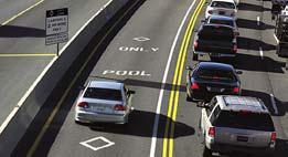
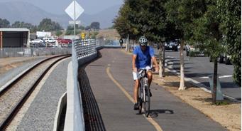
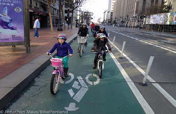
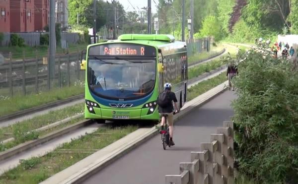
191 October 2018 Unified Corridor Investment Study - DRAFT Step 2 Analysis Page 183

192 Three parallel routes - Highway 1, Soquel/Freedom and the Santa Cruz Branch Rail Line - link the communities along the Santa Cruz County coast from Davenport through Watsonville. The Unified Corridor Study examines how well complimentary transportation improvements on all three routes - when designed to function together as a single unified corridor perform to meet the community s transportation needs. The Unified Corridor Study performance dashboard presents the result of the second, in a two step analysis, which compares how each of the scenarios address the study goals of Safety, Efficiency, Economics, Environmental Sustainability, and Social Equity by The evaluation of 16 performance measures for each of the scenarios and a comparison to a no build and baseline conditions is designed to increase understanding of transportation project benefits by transparently evaluating their impacts and lead to effective investments in the corridor. Unified Corridor Investment Study - DRAFT Step 2 Analysis Page 184

193 Highway 1 Projects Scenario A Scenario B Scenario C Scenario E No Build Buses on shoulders High occupancy vehicle lanes (HOV) and increased transit frequency Auxiliary lanes to extend merging distance IN ADDITION TO MEASURE D Metering of on-ramps Additional lanes on bridge over San Lorenzo River Mission St intersection improvements Soquel Avenue/Drive and Freedom Blvd BRT lite (faster boarding, transit signal priority and queue jumps) Increased frequency of transit with express services Buffered/protected bike lanes Intersection improvements for auto Intersection improvements for bikes/pedestrians Rail Corridor Bike and pedestrian trail Local rail transit with interregional connections Bus rapid transit Freight service on rail Overall Project Area/Connections between Routes Improved bike/pedestrian facilities throughout urban area closing gaps in network Additional transit connections Bike share, bike amenities, transit amenities, park and ride lots Multimodal transportation hubs Automated vehicles/connected vehicles Transportation Demand and System Management Employers and residences - incentive programs Education and enforcement - electric vehicle, motorist safety, and bike safety Only Watsonville These projects will be evaluated in all scenarios. These projects will be evaluated in all scenarios. Unified Corridor Investment Study - DRAFT Step 2 Analysis Page 185

194 This page left intentionally blank. Unified Corridor Investment Study - DRAFT Step 2 Analysis Page 186

195 (Fatal, Injury, and Property Damage Only per year) Scenario A, 3017 No Build, 3265 Baseline, 2916 Highway 1 Projects HOV and auxiliary lanes, ramp meters, San Lorenzo bridge widening, multimodal intersection improvements Soquel / Freedom BRT Lite with increased transit frequency, multimodal intersection improvements Rail ROW Bike and pedestrian trail (mph) Scenario A Scenario A Walk 10.9% Bike 4.3% Transit 4.1% Drive Alone 42.8% AM Peak Period 6:00-9:00 AM Baseline PM Peak Period 4:00-7:00 PM No Build Carpool 37.8% Unified Corridor Investment Study - DRAFT Step 2 Analysis Page 187

196 (In thousands) Scenario A No Build Baseline Seabright Avenue 41st Ave San Andreas/Freedom (In millions) Annual Cost for O&M $20 $7 $13 New Public Investment Needed Funding Potential $520 $379 Capital Costs $899 Scenario A Scenario A (per year in millions) Total Transient Occupancy Tax Visitor Related Sales Tax $40 $39 $29 $28 $27 $18 $10 $12 $12 Baseline Scenario A No Build Unified Corridor Investment Study - DRAFT Step 2 Analysis Page 188

197 (per year) Cost per $224 K Collision x No Build 3,265 Collisions = No Build $730 M Collision Cost Cost per $224 K Collision x Scenario A 3,017 Collisions = Scenario A $675 M Collision Cost Cost -$56 M Savings (Countywide VMT per day in millions) Scenario A 2035 No Build Baseline 5.48 (metric tons per day) Baseline No Build Scenario A CO SOX PM10 PM2.5 ROG NOX Unified Corridor Investment Study - DRAFT Step 2 Analysis Page 189

198 CO 2 e Emissions (metric tons per day) and Percentage Reduction from 2015 Baseline CO 2 e 2,617-27% -26% 1,915 1,941 Baseline No Build Scenario A (# linear miles along 3 routes) nd lowest score (per year in millions) Scenario A No Build 2015 Baseline Unified Corridor Investment Study - DRAFT Step 2 Analysis Page 190

199 Percentage of Income Spent on Transportation (by median income households per year) No Build 18% Baseline 16% No Build 26% Baseline 24% 17% 25% Daily Costs for 2-Vehicle Households Scenario A $ Baseline $46.63 $ No Build $50.14 $ Vehicle Household 2 Vehicle Household 24.0% 13.7% of population is transportation disadvantaged Scenario A Unified Corridor Investment Study - DRAFT Step 2 Analysis Page 191

200 This page left intentionally blank. Unified Corridor Investment Study - DRAFT Step 2 Analysis Page 192

201 (Fatal, Injury, and Property Damage Only per year) Scenario B, 2899 No Build, 3265 Baseline, 2916 Highway 1 Projects Bus on shoulder, ramp metering, Mission St. intersection improvements Soquel / Freedom BRT Lite with increased transit frequency, buffered/protected bike lanes, bike/ped intersection improvements Rail ROW Bike and pedestrian trail, rail transit (mph) Scenario B Scenario B Bike 4.4% Walk 10.7% Drive Alone 42.4% AM Peak Period 6:00-9:00 AM Baseline PM Peak Period 4:00-7:00 PM No Build Transit 6.0% Carpool 36.5% Unified Corridor Investment Study - DRAFT Step 2 Analysis Page 193

202 (In thousands) Scenario B No Build Baseline Seabright Avenue 41st Ave San Andreas/Freedom (In millions) Annual Cost for O&M $44 $9 $35 New Public Investment Needed Funding Potential $379 $455 Capital Costs $833 Scenario B Scenario B (per year in millions) Total Transient Occupancy Tax Visitor Related Sales Tax $40 $39 $29 $28 $27 $18 $10 $12 $12 Baseline Scenario B No Build Unified Corridor Investment Study - DRAFT Step 2 Analysis Page 194

203 (per year) Cost per $224 K Collision x No Build 3,265 Collisions = No Build $730 M Collision Cost Cost per $224 K Collision x Scenario B 2,899 Collisions = Scenario B $649 M Collision Cost Cost -$82 M Savings (Countywide VMT per day in millions) Scenario B 2035 No Build Baseline 5.48 (metric tons per day) Baseline No Build Scenario B CO SOX PM10 PM2.5 ROG NOX Unified Corridor Investment Study - DRAFT Step 2 Analysis Page 195

204 CO 2 e Emissions (metric tons per day) and Percentage Reduction from 2015 Baseline CO 2 e 2,617-27% -28% 1,915 1,886 Baseline No Build Scenario B (# linear miles along 3 routes) nd highest score (per year in millions) Scenario B No Build 2015 Baseline Unified Corridor Investment Study - DRAFT Step 2 Analysis Page 196

205 Percentage of Income Spent on Transportation (by median income households per year) No Build 18% Baseline 16% No Build 26% Baseline 24% 17% 25% Daily Costs for 2-Vehicle Households Scenario B $ Baseline $46.63 $ No Build $50.14 $ Vehicle Household 2 Vehicle Household 25.2% 13.7% of population is transportation disadvantaged Scenario B Unified Corridor Investment Study - DRAFT Step 2 Analysis Page 197

206 This page left intentionally blank. Unified Corridor Investment Study - DRAFT Step 2 Analysis Page 198

207 (Fatal, Injury, and Property Damage Only per year) Scenario C, 3013 No Build, 3265 Baseline, 2916 Highway 1 Projects Bus on shoulders, auxiliary lanes Soquel / Freedom BRT Lite with increased transit frequency, multimodal intersection improvements Rail ROW Bike and pedestrian trail, bus rapid transit, freight service (in Watsonville) (mph) Scenario C Scenario C Bike 4.2% Walk 10.8% Drive Alone 43.1% AM Peak Period 6:00-9:00 AM Baseline PM Peak Period 4:00-7:00 PM No Build Transit 4.8% Carpool 37.1% Unified Corridor Investment Study - DRAFT Step 2 Analysis Page 199

208 (In thousands) Scenario C No Build Baseline Seabright Avenue 41st Ave San Andreas/Freedom (In millions) Annual Cost for O&M $28 $6 $22 New Public Investment Needed Funding Potential $285 $455 Capital Costs $740 Scenario C Scenario C (per year in millions) Total Transient Occupancy Tax Visitor Related Sales Tax $40 $39 $29 $28 $27 $18 $10 $12 $12 Baseline Scenario C No Build Unified Corridor Investment Study - DRAFT Step 2 Analysis Page 200

209 (per year) Cost per $224 K Collision x No Build 3,265 Collisions = No Build $730 M Collision Cost Cost per $224 K Collision x Scenario C 3,013 Collisions = Scenario C $674 M Collision Cost Cost -$56 M Savings (Countywide VMT per day in millions) Scenario C 2035 No Build Baseline 5.48 (metric tons per day) Baseline No Build Scenario C CO SOX PM10 PM2.5 ROG NOX Unified Corridor Investment Study - DRAFT Step 2 Analysis Page 201

210 CO 2 e Emissions (metric tons per day) and Percentage Reduction from 2015 Baseline CO 2 e 2,617-27% -27% 1,915 1,899 Baseline No Build Scenario C (# linear miles along 3 routes) 36.0 Lowest score (per year in millions) Scenario C No Build 2015 Baseline Unified Corridor Investment Study - DRAFT Step 2 Analysis Page 202

211 Percentage of Income Spent on Transportation (by median income households per year) No Build 18% Baseline 16% No Build 26% Baseline 24% 17% 25% Daily Costs for 2-Vehicle Households Scenario C $ Baseline $46.63 $ No Build $50.14 $ Vehicle Household 2 Vehicle Household 25.2% 13.7% of population is transportation disadvantaged Scenario C Unified Corridor Investment Study - DRAFT Step 2 Analysis Page 203

212 This page left intentionally blank. Unified Corridor Investment Study - DRAFT Step 2 Analysis Page 204

213 (Fatal, Injury, and Property Damage Only per year) Scenario E, 3008 No Build, 3265 Highway 1 Projects HOV and auxiliary lanes, ramp meters Soquel / Freedom Buffered/protected bike lanes, bike/pedestrian intersection improvements Rail ROW Bike and pedestrian trail, rail transit, freight service Baseline, 2916 (mph) Scenario E Scenario E Bike 4.4% Walk 10.7% Drive Alone 42.3% AM Peak Period 6:00-9:00 AM Baseline PM Peak Period 4:00-7:00 PM No Build Transit 5.3% Carpool 37.3% Unified Corridor Investment Study - DRAFT Step 2 Analysis Page 205

214 (In thousands) Scenario E No Build Baseline Seabright Avenue 41st Ave San Andreas/Freedom (In millions) $1 Annual Cost for O&M $32 $32 New Public Investment Needed Funding Potential $794 $453 Capital Costs $1,247 Scenario E Scenario E (per year in millions) Total Transient Occupancy Tax Visitor Related Sales Tax $40 $39 $29 $28 $27 $18 $10 $12 $12 Baseline Scenario E No Build Unified Corridor Investment Study - DRAFT Step 2 Analysis Page 206

215 (per year) Cost per $224 K Collision x No Build 3,265 Collisions = No Build $730 M Collision Cost Cost per $224 K Collision x Scenario E 3,008 Collisions = Scenario E $673 M Collision Cost Cost -$58 M Savings (Countywide VMT per day in millions) Scenario E 2035 No Build Baseline 5.48 (metric tons per day) Baseline No Build Scenario E CO SOX PM10 PM2.5 ROG NOX Unified Corridor Investment Study - DRAFT Step 2 Analysis Page 207

216 CO 2 e Emissions (metric tons per day) and Percentage Reduction from 2015 Baseline CO 2 e 2,617-27% -26% 1,915 1,928 Baseline No Build Scenario E (# linear miles along 3 routes) 40.7 Highest score (per year in millions) Scenario E No Build 2015 Baseline Unified Corridor Investment Study - DRAFT Step 2 Analysis Page 208