Status of the Kelp Beds 2010

Transcription

1 Status of the Kelp Beds 2010 Ventura Los Angeles Orange Counties Central Region Kelp Survey Consortium June 2011 Prepared by: MBC Applied Environmental Sciences Costa Mesa, California

2

3 Status of the Kelp Beds 2010 Ventura Los Angeles Orange Counties Central Region Kelp Survey Consortium June 2011 Prepared by: MBC Applied Environmental Sciences 3000 Red Hill Avenue Costa Mesa, California 92626

4 PROJECT STAFF Central Region Kelp Survey Consortium Gerald McGowen, City of Los Angeles Bureau of Sanitation, Hyperion Treatment Plant Mark Pumford, City of Oxnard Wastewater Treatment Plant Shelly Walther, Los Angeles County Sanitation Districts Katherine Rubin, Los Angeles Department of Water and Power Alex Sanchez, NRG, El Segundo Operations Inc. Michael Mengel, Orange County Sanitation Districts Wayne Ishimoto, Chevron Products Company William Baker, GenOn Energy MBC Applied Environmental Sciences Project Manager M. D. Curtis Marine Scientists D. S. Beck M. D. Curtis C. T. Mitchell K. L. Mitchell R.H. Moore M. R. Pavlick J. L. Rankin B.L. Smith Cover Photograph Courtesy of Eric Hanauer

5 TABLE OF CONTENTS Page LIST OF FIGURES iv LIST OF TABLES v EXECUTIVE SUMMARY vi INTRODUCTION KELP LIFE HISTORY ENVIRONMENTAL DETERMINANTS OF KELP GROWTH PREDICTING POTENTIAL GROWTH KELP BED SUMMARY CENTRAL REGION KELP BEDS GENERAL OVERVIEW SURVEY YEAR - RESULTS OF THE SURVEYS UPDATE TO THE PRESENT STATUS OF THE 27 KELP BEDS IN 2010 AND CRKSC NORTH (Ventura River Mouth to Point Mugu) FISH AND GAME KELP BED 17 (Point Mugu to Point Dume) FISH AND GAME KELP BED 16 (Point Dume to Malibu Point) FISH AND GAME KELP BED 15 (Malibu Point to Santa Monica Pier) CRKSC CENTRAL (Santa Monica Pier to Redondo Beach Breakwater Southern Tip) FISH AND GAME KELP BEDS 14 (Malaga Cove to Point Vincente) AND 13 (Point Vicente to San Pedro Breakwater) CRKSC SOUTH (San Pedro Breakwater Lighthouse to Laguna Beach) DISCUSSION CONCLUSION LITERATURE CITED PERSONAL COMMUNICATIONS WEB SITES APPENDICES Appendix A Appendix B Appendix C Appendix D Kelp Canopy Maps Historic Coverage Area of Kelp Canopies Flight Data Reports Kelp Canopy Aerial Photographs

6 Status of the Kelp Beds 2010 CRKSC Report 2011 LIST OF FIGURES iv Page Figure 1. Ocean dischargers located within the Central Region Kelp Survey Consortium program area Figure 2. Kelp life cycle Figure 3. Multivariate ENSO Index from 1950 through Figure 4. SST stations (TN and TM in green) along the Palos Verdes Peninsula Figure 5. Combined canopy coverage at all kelp beds in Central Region from Ventura to Laguna Beach Figure 6. SSTs from five Central Region monitoring locations superimposed on the SIO harmonic equation Figure 7. Daily sea surface temperatures (SST) offshore Point Dume for 2010 and through mid- May Figure 8. Daily sea surface temperatures (SST) Station TM offshore Palos Verdes for 2010 and through March Figure 9. Daily sea surface temperatures (SST) at Station TN offshore Palos Verdes for 2010 and through March Figure 10. Daily sea surface temperatures (SST) at Santa Monica Pier for 2010 and through 26 May Figure 11. Daily sea surface temperatures (SST) from Newport Pier for 2010 and through April Figure 12. Significant wave heights offshore San Pedro, CA. 1 January 2010 through 11 May Figure 13. Significant wave heights offshore Santa Monica, CA. 1 January 2010 through 11 May Figure 14. SSTs from all Central Region Stations in Figure 15. Comparisons between the average Northern and Central Los Angeles County ABAPY and the canopy coverage of the kelp bed off Deer Creek for the years shown Figure 16. Comparisons between the average Northern and Central Los Angeles County ABAPY and the canopy coverage of the kelp bed off Leo Carillo for the years shown Figure 17. Comparisons between the average Northern and Central Los Angeles County ABAPY and the canopy coverage of the kelp bed off Nicolas Canyon for the years shown Figure 18. Comparisons between the average Northern and Central Los Angeles County ABAPY and the canopy coverage of the kelp bed off El Pesc/La Pied for the years shown Figure 19. Comparisons between the average Northern and Central Los Angeles County ABAPY and the canopy coverage of the kelp bed off Lechuza for the years shown Figure 20. Comparisons between the average Northern and Central Los Angeles County ABAPY and the canopy coverage of the kelp bed off Pt. Dume for the years shown Figure 21. Comparisons between the average Northern and Central Los Angeles County ABAPY and the canopy coverage of the kelp bed off Paradise Cove for the years shown Figure 22. Comparisons between the average Northern and Central Los Angeles County ABAPY and the canopy coverage of the kelp bed off Escondido Wash for the years shown Figure 23. Comparisons between the average Northern and Central Los Angeles County ABAPY and the canopy coverage of the kelp bed off Latigo Canyon for the years shown Figure 24. Comparisons between the average Northern and Central Los Angeles County ABAPY and the canopy coverage of the kelp bed off Puerco/Amarillo for the years shown Figure 25. Comparisons between the average Northern and Central Los Angeles County ABAPY and the canopy coverage of the kelp bed off Malibu Pt. for the years shown Figure 26. Comparisons between the average Northern and Central Los Angeles County ABAPY and the canopy coverage of the kelp bed off La Costa for the years shown Figure 27. Comparisons between the average Northern and Central Los Angeles County ABAPY and the canopy coverage of the kelp bed off Las Flores for the years shown Figure 28. Comparisons between the average Northern and Central Los Angeles County ABAPY and the canopy coverage of the kelp bed off Big Rock for the years shown

7 Status of the Kelp Beds 2010 CRKSC Report 2011 v Figure 29. Figure 30. Figure 31. Figure 32. Figure 33. Figure 34. Figure 35. Figure 36. Figure 37. Figure 38. Comparisons between the average Northern and Central Los Angeles County ABAPY and the canopy coverage of the kelp bed off Las Tunas for the years shown Comparisons between the average Northern and Central Los Angeles County ABAPY and the canopy coverage of the kelp bed off Topanga for the years shown Comparisons between the average Palos Verdes and Cabrillo ABAPY and the canopy coverage of the kelp bed off PV IV for the years shown Comparisons between the average Palos Verdes and Cabrillo ABAPY and the canopy coverage of the kelp bed off PV III for the years shown Comparisons between the average Palos Verdes and Cabrillo ABAPY and the canopy coverage of the kelp bed off PV II for the years shown Comparisons between the average Palos Verdes and Cabrillo ABAPY and the canopy coverage of the kelp bed off PV I for the years shown Comparisons between the average Palos Verdes and Cabrillo ABAPY and the canopy coverage of the kelp bed off Cabrillo for the years shown Comparisons between the average Palos Verdes and Cabrillo ABAPY and the canopy coverage of the kelp bed off POLA-POLB Harbor for the years shown Comparisons between the average Orange County ABAPY and the canopy coverage of the kelp bed off the Newport-Irvine Coast for the years shown Comparisons between the average Orange County ABAPY with the history of Laguna Beach kelp (i.e., the sums of canopy coverage for North Laguna Beach plus South Laguna Beach kelp) for the years shown LIST OF TABLES Table 1. Seasonal kelp nutritional index based on weighting values given to monthly temperature data derived from Santa Monica Pier (SMP), indicated in parenthesis, and Newport Pier(NP). The weighting values are derived from nitrate versus temperature data from North and Jones (1991), and nitrate uptake rates from Haines and Wheeler (1978), and Gerard (1982). The season begins 1 July and ends 30 June. Years in Red denote warm-water years, Blue cold-water years, both colors are transition years, based on NOAA Multivariate ENSO Index (MEI), May Table 2. Historical canopy coverage in km² of Ventura, Los Angeles, and Orange County kelp beds to Newport Beach, from 1911 to Values represent an estimate of coverage utilizing varying methods over the years. Areal estimates for were derived from infrared aerial photographs. Data for years 1959, 1963, 1971, and 1976 appear in Appendix B Table 3. Rankings assigned to the 2010 aerial photograph surveys of the Ventura, Los Angeles, and Orange County kelp beds, and rankings assigned to an April 2011 aerial survey. The basis for a ranking was the status of a canopy during surveys from recent years, excluding periods of El Niño or La Niña conditions or following exceptional storms. A ranking of 2.5 would represent the average status Table 4. Historical record of kelp canopy coverage of the Palos Verdes Peninsula

8 STATUS OF THE KELP BEDS 2010 VENTURA, LOS ANGELES, AND ORANGE COUNTIES CENTRAL REGION KELP SURVEY CONSORTIUM JUNE 2011 EXECUTIVE SUMMARY Foreword. Continuing favorable environmental factors contributed to the maintenance of giant kelp offshore of the Central Region in The 2010 giant kelp study demonstrated that oceanographic factors during a prolonged La Niña such as the availability of nutrients (or lack thereof) continued to control the fate of the kelp beds in There was no evidence to suggest that any of the region s various dischargers had any perceptible influence on the persistence of the region s giant kelp beds. Formation of the Central Region Kelp Survey Consortium. The Central Region Kelp Survey Consortium (CRKSC) was formed in late 2002 with the purpose of fulfilling Los Angeles Regional Water Control Board (LARWQCB) requirements for its ocean dischargers to form a regional kelp bed-monitoring program. The LARWQCB stated that participation would be a monitoring component in renewed National Pollution Discharge Elimination System (NPDES) permits for ocean dischargers within their jurisdiction. A series of meetings with a group of ocean dischargers and the LARWQCB within the region were held in 2002 to discuss the design and implementation of the regional kelp bed monitoring program. Representatives of Publicly Owned Treatment Works (POTWs), power generators, storm water agencies, and non-governmental organizations participated, including one POTW outside of the LARWQCB jurisdictional boundaries (Orange County Sanitation District). Six organizations agreed to form the Central Region Kelp Survey Consortium (CRKSC) to develop, fund, and implement a survey to begin in In 2005, a seventh member, the Los Angeles Bureau of Sanitation Hyperion Treatment Plant, was added as a required member. It was agreed among the funding participants and the LARWQCB that the monitoring program would be methodologically based upon, and coordinated with, the Region Nine Kelp Survey Consortium. With the CRKSC program (since 2003) and the Region Nine program (since 1982) combined, all coastal kelp beds from the Ventura-Los Angeles County line to the Mexican Border are surveyed synoptically several times a year, a coverage of approximately 220 of the 270 miles of the southern California mainland coast. Aerial Flights Aerial surveys of the giant kelp beds from the Santa Barbara-Ventura County line to Newport Harbor were conducted in 2010 by MBC Applied Environmental Sciences (MBC). The surveys in 2010 were conducted on 28 March, 22 August, 4 November, and 31 December 2010; the survey or surveys that showed the kelp beds in the region at their greatest extent were analyzed, quantified, and depicted on appropriate site maps. One aerial survey has also been completed for the 2011 survey year on 16 April and three more will be conducted throughout the remainder of Flight conditions were relatively good during all the surveys. Reasonable attempts were made to conduct one aerial overflight within each of the four quarters in the year; however, 2010 was the year without a summer. A persistent marine layer with low-lying clouds prevented surveys from late-june until mid-august causing a 1.5 month longer gap in the record than planned. Due to the delay, the next two surveys were scheduled to split the remaining time, with the third survey scheduled for late-october (weather pushed that survey to 4 November), and the last for late-december. Based on the results of the surveys, maximum canopy coverage throughout most of the region was observed during the flight of 31 December (or the 22 August and 4 November flights for the Palos Verdes kelp beds). Although kelp beds were generally smaller in 2010, they had all increased from the lows observed in the last half of These kelp beds were generally larger by the late-march 2010 survey than that reported in December Most increased again during the August 2010 survey (and all maintained canopies which is unusual for summer surveys), about one-half increased by the November 2010 survey, and then increased to their maximums by the December 2010 survey (a significant fraction of what was observed during 2009 surveys).

9 Status of the Kelp Beds 2010 CRKSC Report 2011 vii Oceanographic Environment The National Oceanic and Atmospheric Administration (NOAA) indicates that 2010 was a La Niña year following a mild El Niño in Historic Sea Surface Temperatures (SSTs) from Point Dume, Santa Monica Pier, two stations at Palos Verdes, and Newport Pier were used to determine the availability of nutrients in the region. All stations were in synchrony (with rare exceptions) in both the northern and southern portions of the Central Region reacting in a similar manner to similar temperature pulses throughout the year. However, in June and July the SSTs at the Palos Verdes sampling station (TN), located at the north end of Palos Verdes, were much cooler than average and cooler than the other stations in the Central Region. From January through February, temperatures were warmer than average, but giving way to cooler waters through May. All stations (although warmer) stayed much cooler than average through the summer until mid-september whereupon they stayed warmer, but average, until late-october/early- November, with cool temperatures predominating in the region through December. As a result of the cooler SSTs, most of the CRKSC kelp beds expanded to a significant fraction or greater than what they were in earlyto-mid Water clarity was relatively favorable for kelp growth in 2010; rainfall totals were at normal levels in the region, but the contrast from drought made it appear higher and there were relatively short duration periods when the rivers and streams emptied into the ocean making the nearshore waters turbid. Algal blooms occurred but did not persist long enough to seriously affect photosynthetic opportunities and did not appear to contribute to any stress on the kelp beds. In general, turbidity from storms, rainfall, and phytoplankton blooms did not appear to be a factor in the growth of kelp canopy in Typical swell sizes and directions were observed through most of 2010, with swells generally approaching the region from the south and west. Buoy data from January, February, and April recorded high-energy waves up to 4.4 m (14.5 ft) in height approaching from the west in early January 2010 at San Pedro. Other large swells of 3.8 m, 3.75 m, and 3.7 m height occurred again at San Pedro in January and February and a 3.7-m swell occurred in early-april at the Santa Monica Bay buoy. Seas were relatively calm after that until late-december when large swells of 3.5 m were again recorded. Therefore, wave and swell intensity probably contributed to stresses upon the giant kelp resources. Fortunately, no particularly large waves occurred during the summer when most of the kelp beds were somewhat stressed throughout the Central Region. Giant Kelp Survey Results Results of the 2010 CRKSC survey estimates that the maximum measured kelp canopy decreased significantly from square kilometers (km 2 ) in 2009 to km 2 in 2010 (Table 2). The number of kelp beds displaying canopy have remained markedly similar and with the addition of two more beds in 2009 in Orange County, the total number of beds monitored for the Central Region is 27 historic or extant kelp beds. The total amount of kelp present was greater than during any past CRKSC survey other than the very large 2009 survey and of any past synoptic surveys (all CRKSC areas sampled) conducted since The large-scale changes to the kelp beds noted are typically responses to ENSO (El Niño or La Niña) events, while the finer-scale variation observed in prior years indicates there still remains variation due to multi-decadal effects/regime changes within a region that we cannot yet accurately predict with our current knowledge. In spite of this uncertainty in our predictive ability, the kelp beds of the Central Region in 2010 recorded increases from the minor-el Niño that perturbed the Central Region beds in mid-to-late 2009, indicating the resiliency observed during the past eight monitoring years. As far as the greatest extent of canopy coverage during the quarterly surveys, 2010 was typical in that the December survey depicted most of the region s kelp beds at their greatest extent (with the exception of the Palos Verdes beds which reached maximums in August and November) (Appendix A). Throughout the entire study area, kelp canopy coverage decreased but not uniformly, with distribution of kelp among the region s 27 kelp beds (only 24 are extant beds, as three, Sunset, Horseshoe, and Huntington Flats, have been missing for decades) varying widely. The larger beds generally saw the largest decreases, with Deer Creek beds losing 40% of its area and Palos Verdes IV losing almost 1km 2, while PV I lost almost 0.6 km 2. Many

10 Status of the Kelp Beds 2010 CRKSC Report 2011 viii mid-to-smaller sized beds either stayed the same or actually increased in The five CRKSC beds of F&G Bed No. 17 decreased from km 2 to km 2 and the six beds comprising F&G Bed No.16 decreased only slightly from km 2 to km 2. F&G Bed No. 15 increased, but as the beds that comprised it were very small, little change was noted among the six beds increasing from km 2 to km 2. F&G Bed No. 14 decreased with the Palos Verdes Beds IV and Bed III decreasing from km 2 in 2010 to km 2 in 2010; F&G Bed No. 13 (encompassing the shoreline from Point Vicente to the Los Angeles Harbor Breakwater) decreased from km 2 to km 2. In total, the Palos Verdes kelp beds decreased in 2010 from that recorded in 2009, from km 2 to km 2. F&G Bed No. 12 from Newport to past-laguna Beach grew greatly from km 2 to km 2 again pointing out differences a few miles of coastline with varying oceanographic regimes can have on the extant kelp resources. Conclusion 2010.The giant kelp survey of 2010 continued to demonstrate that kelp bed dynamics in the Central Region are controlled by the large-scale oceanographic environment. None of the kelp beds in the region reacted contrary to what was observed region wide. There was no evidence of any adverse effects on the giant kelp resources from any of the region s dischargers. The remarkable recovery of the kelp beds over the past six years could be augmented in 2011 as nutrients appear to be replete in the region, but El Niño neutral conditions are forecast for the remainder of the 2011 year.

11 STATUS OF THE KELP BEDS 2010 VENTURA, LOS ANGELES, AND ORANGE COUNTIES CENTRAL REGION KELP SURVEY CONSORTIUM June 2011 INTRODUCTION In 2010, aerial surveys of the giant kelp beds from the northern Ventura County line to Newport Harbor were conducted by MBC Applied Environmental Sciences (MBC) for the Central Region Kelp Survey Consortium (CRKSC). From these surveys, conducted on 28 March, 22 August, 4 November, and 31 December 2010, the survey or surveys that showed the kelp beds in the region at their greatest extent were analyzed, quantified, and depicted on appropriate site maps (Appendix A). A map showing the geographical range and the ocean dischargers located within the CRKSC region is shown in Figure 1. Figure 1. Ocean dischargers located within the Central Region Kelp Survey Consortium program area. KELP LIFE HISTORY Kelp consists of a number of species of brown algae of which 10 are typically found from the Mexican Border to Point Conception (Southern California Bight [SCB]). Compared to most other algae, kelp species can attain remarkable size and long life span (Kain 1979, Dayton 1985, Reed et al. 2006). Along the southern and central California coast, giant kelp (Macrocystis pyrifera) is the largest species colonizing rocky (and in some cases sandy) subtidal habitats. Giant kelp is a very important component of coastal and island communities in southern California, providing food and habitat for numerous animals (North 1971, Foster and Schiel 1985, Dayton 1985). A sizable literature on Macrocystis biology and ecology began a century ago, with much effort spent in the early years deciphering its enigmatic life history (Neushul 1963, North 1971, Dayton 1985, Schiel and Foster 1986, Witman and Dayton 2001, Reed et al. 2006). Darwin (1860) noted the resemblance of the three-dimensional structure of kelp stands to that of terrestrial forests.

12 Status of the Kelp Beds 2010 CRKSC Report Giant kelp commonly attains lengths of 50 to 75 ft and can be found at depths of up to 90 ft. In conditions of unusually good water clarity, giant kelp may even thrive to depths of 150 ft. Giant kelp forms beds wherever suitable substrate occurs, typically on rocky subtidal reefs. Such substrate must usually be free of continuous sediment intrusion. Giant kelp beds can form in sandy bottom habitats where individuals will attach to worm tubes, given that the area is protected from direct swells as is seen along portions of the Santa Barbara coastline. Like plants, algae undergo photosynthesis and therefore require light energy to generate sugars. For this reason, light availability at depth is an important limiting factor to kelp growth. Greater water clarity normally occurs at the offshore islands, and as a result, giant kelp is commonly found growing in depths exceeding 100 ft. Along the mainland coast, high productivity, terrestrial inputs and continental shelf mixing result in greater turbidity and hence lower light levels as through attenuation. Consequently, kelp generally does not grow deeper than 60 ft along the coastal shelf, although exceptional conditions in San Diego produce impressively large beds that can grow vigorously beyond 100 ft. Giant kelp has a complex life cycle and undergoes a heteromorphic alternation of generation, where the phenotypic expression of each generation does not resemble the generation before or after it (Figure 2). The stage of giant kelp that is most familiar is the adult canopy-forming diploid sporophyte generation. Sporophyll blades at the base of an adult giant kelp release zoospores, especially in the presence of cold nutrient-rich waters. These zoospores disperse into the water column and generally settle a short distance from the parent sporophyte. Within three weeks, the zoospores mature into microscopic male and female gametophytes. This second generation does not resemble the sporophyte. Sperm and eggs are released into the water column where fertilization occurs. Dispersal distance can be greater during this phase compared to the zoospore stage. The life cycle is completed when a fertilized egg settles and develops into the adult sporophyte stage. Successful completion of the life cycle relies on the persistence of favorable conditions throughout the process. Giant kelp is known as a biological facilitator (sensu Bruno and Bertness 2001), where its three-dimensional structure and the complexity of its holdfast provides substrate, refuge, reduction of physical stress, and a food source for many fish (Carr 1989) and invertebrates (Duggins et al. 1990). Stands of kelp can also affect flow characteristics in the nearshore zone, thus enhancing recruitment (Duggins et al. 1990), which further acts to increase animal biomass in the vicinity. For these reasons, giant kelp is also of great importance to sport and commercial fisheries. ENVIRONMENTAL DETERMINANTS OF KELP GROWTH Giant kelp bed size and health is known to be highly variable but there has been a downward trend from the inception of surveying in 1911 and the end of the century. During this period kelp beds declined at Figure 2. Kelp life cycle. most coastal and island sites in the SCB. A comprehensive historical review of kelp beds in the SCB (Neushul 1981) found that an approximately one-third loss of kelp bed cover had occurred since 1911 when compared to a 25-year mean. A statewide survey in 1989 (Ecoscan 1990) estimated Southern California kelp forests to total 10,360 ha (103.6 km 2 ) (Tarpley and Glantz 1992), a 25% reduction from that reported by Crandall (138 km 2 ) in 1911 (from Neushul 1981). Measurements that Crandall took of the Central Region kelp beds in 1911 indicated that total coverage was about 18 km 2. This total was probably larger in 1928 based on the size of the Palos Verdes beds which were then km 2 as compared to the km 2 that Crandall measured in 1910, but data was not taken for the remainder of the Central Region so no definitive

13 Status of the Kelp Beds 2010 CRKSC Report regional total was available. The next complete survey of the region was not until 1955 which indicated the beds had decreased by almost two-thirds, to about 7 km 2 from that recorded in The most significant loss was that of the Palos Verdes beds which had decreased by almost 90%. By 1967, a total of almost 8 km 2 indicated slight improvements, but Palos Verdes kelp beds were still very small. Surveys in 1972 and 1975 recorded further losses with kelp canopy totals down to 3.5 km 2. The impetus by the 1989 La Niña resulted in almost 6 km 2 of kelp canopy, but kelp totals decreased to about one half this during the subsequent two decades. In 2009, favorable conditions again increased canopy total to about 6.5 km 2, larger than it had been since As these measurements indicate most of the beds remain smaller than those of a century ago, we attempt herein to determine what environmental factors have changed in the intervening years to cause such large declines. Many factors determine whether giant kelp will recruit successfully, form a bed in a given area, and persist. These include the obvious factors such as available habitat, adequate light, nutrient availability, exposure to currents, prevailing swells, storms, predator-prey interactions, and the presence of herbivores. We also know that there are less obvious but potentially more far reaching effects in both time and scope such as the El Niño Southern Oscillation (ENSO) (referring to global climatic changes and effects), decadal regime shifts or climate shifts/variation (Miller et al. 1994, Breaker and Flora 2009), the Pacific Decadal Oscillation (referring to events that are Pacific wide and decades long in nature), and the El Niño/La Niña events (which refer to more local effects resulting in warming or cooling of the waters along the South and North American western coast). Light. Primarily, kelp needs adequate light conditions to photosynthesize and the amount of light available can be affected by physical and biological factors. Prolonged conditions of turbidity resulting from terrestrial run-off, especially during lengthy rainstorms, can reduce kelp growth. Phytoplankton blooms are typical in the spring and fall due to the supply of nutrients into the inshore waters from upwelling, but blooms of phytoplankton can also sufficiently occlude light that they negatively impact kelp health. Phytoplankton blooms were probably responsible for a large decrease in canopy coverage in 2005 that continued into 2006; fortunately run-off and phytoplankton blooms did not have a serious deleterious effect on the kelp beds through Nutrients. In addition to light, kelp also requires nitrates and other materials in solution to spur adequate growth (Jackson 1977, Haines and Wheeler, 1978, Dayton et al. 1999). Nutrient availability is known to be one of the primary limiting factors to algal growth (Jackson 1977, Zimmerman and Kremer 1984). Unlike terrestrial plants that absorb nutrients only though roots, kelp absorbs nutrients directly through its tissues. Nutrients are generally recycled in the environment through the continuous raining of accumulated organic matter from the shallow sunlit depths to deeper colder waters. Typically the concentration of nitrates increases with depth (Sverdrup et al. 1942). However, shallow waters at depths where kelp commonly occurs tend to have higher temperatures due to solar insolation, and are typically devoid of nutrients. This is due to the abundance of phytoplankton in the surface waters which compete for nutrients in surface waters where light penetration is good. This presents a physiological challenge for giant kelp, which must compete for nutrients and light. In typical, low nutrient conditions generally encountered during the summer, giant kelp will persist only if it can adequately translocate nitrates from below the thermocline through its tissues (Jackson 1977). If the thermocline is depressed (along with nutrients) below the level where kelp is found for an extended period of time, extirpation of the kelp will occur. For this reason, kelp thrives best during periods of upwelling, where deeper, nutrient-rich waters rise from depths where light levels are too low to permit nutrient stripping by phytoplankton. Coastal upwelling events are usually wind-driven phenomena in southern California (such as periods of Santa Ana Winds) where surface friction from prevailing winds from the north creates a southward flow due to Ekman transport (Pond and Picard 1983). As the warmer surface layer is moved offshore, colder bottom water rises from the depths to take its place, especially at the continental margin or near submarine canyons, but in areas with persistent winds close to shore, smaller upwelling events occur in shallower waters. Upwelled waters are typically much colder than surface waters, so temperature tends to correlate with nutrient availability in coastal zones. Studies demonstrating a correlation between the health of kelp beds and surface cooling events are numerous (e.g., Jackson 1977, Tegner et al. 1996, Dayton et al. 1999, and others). Upwelling in southern

14 Status of the Kelp Beds 2010 CRKSC Report California generally occurs during the spring months, although canopy growth is also seen in late fall and winter when the nearshore water column is well mixed. Because of the strong correlation between temperature and kelp growth, episodic El Niño warm water events can have a severe negative impact on the health of kelp beds in the SCB. Surface temperatures above 17 C (64 F) generally indicate waters with very low nutrient content (North and Jones 1991). With roughly each one degree centigrade temperature drop (1.9 F), the availability of nitrates essentially doubles. Therefore, at a temperature of 12 C (54 F), 14 times more nutrients are theoretically available than at C (62-64 F). Storms. Many other physical factors can sometimes impart greater regional influence. For example, storms can hinder or stimulate kelp growth, depending upon how large they are and how much energy they contain. Waves cause a back and forth motion to the kelp; large swells increase the severity of this motion increasing the drag force on the kelp and can break fronds or even dislodge an entire giant kelp. As the fronds of giant kelp often entangle with other nearby giant kelp, the added drag of other loose giant kelp can overpower a more firmly attached neighbor and rip its holdfast free. As these accumulate, there is an increasing drag force on each neighbor causing them to be ripped free of their attachment to the bottom. The resultant mass of entangled, loose giant kelp can drift through a kelp bed ripping out 100s or 1,000s of giant kelp that wash ashore or become a floating kelp paddy offshore (Dayton and Tegner 1984, Ebeling et al. 1985, Seymour et al. 1989). Large storms with catastrophic wave energies, noted in 1983 and 1988, devastated the kelp beds. There is an apparent increasing frequency of El Niños (Boersma 1998) or of a general thermal regime shift (Fiedler 2002). The ramifications of more intense and more frequent El Niño conditions include a potential increase in the frequency of damaging storms that can take out whole kelp beds. Conversely, these large storms have been shown to clear reefs of multistory algal and invertebrate coverage (thereby eliminating competition for space), sweep sediments from underlying bedrock, and they can be a factor in the expansion of a bed by opening habitat not previously available for colonization by giant kelp (MBC 1990). Even though large storms generally are devastating to the kelp bed resources, the twofold factors of the 200-Year Great Storm of 1988 combined with the La Niña of 1989 produced kelp beds in areas that had been devoid of kelp for years, probably as the result of wave energy abrading the multilayered invertebrate coverage and exposure of bed rock for spore colonization (Appendix B). Storm intensity is monitored by the severity of swells. Of particular concern are storms that produce swell heights that exceed 4 m. In the shallow nearshore zone where waves are influenced by the sea bottom, the resulting motion becomes increasingly more horizontal as waves approach the shore. Grazing. Another physical factor includes kelp herbivores; therefore monitoring their status or the status of their predators can be important factors in determining checks on kelp growth. A reduction in natural predators will allow herbivores such as urchins to proliferate unchecked, resulting in overgrazing of kelp (North 1983, Wilson and Togstad 1983, Dayton 1985, Harrold and Reed 1985, Harrold and Pearse 1987, Murray and Bray 1993). These have been implicated in wholesale loss of kelp beds at Palos Verdes, San Mateo Point, and Imperial Beach, and large detrimental effects on many other kelp beds (North and Jones 1991). Anthropogenic Effects. Large-scale oceanographic cycles such as ENSO events are monitored closely, and the ability of existing models to predict the onset of conditions that are either significantly warmer or colder than average increases every year as the profusion and quality of data increases. For this reason, it is far easier to correlate the variability of kelp bed abundance and health to natural physical phenomena than it is to relate it to anthropogenic causes. Anthropogenic effects on kelp beds have been documented, most notably the pollution-related loss of kelp beds offshore of Palos Verdes (from the late1950s through much of the 1970s) and Point Loma (in the mid-1990s) (SWQCB 1964, North 1968, Meistrell and Montagne 1983). It appears the cause of the loss of kelp at the Point Loma outfall (possibly related to a broken pipe discharging sewage) was not the sewage, but probably the accompanying turbidity (North 2001). Other factors have included unchecked runoff from coastal construction projects such as what appeared to have occurred during construction of Interstate 5 in the late-1960s (loss of Barn Kelp for several years), and construction of homes at Salt Creek in the late-1970s which resulted in the loss of the large kelp bed (Salt Creek-Dana Point Kelp) located directly offshore for several years (North and MBC 2001).

15 Status of the Kelp Beds 2010 CRKSC Report Unfamiliarity with the ecological consequences of overfishing affecting fisheries within kelp forests have also contributed to predator-prey inequalities (Tegner and Dayton 2000). Historically, these anthropogenic losses would also include the loss of the Horseshoe Kelp bed offshore of San Pedro Harbor in the late-1930s. This loss was probably from turbidity due to an increasing population and dumping of sediment from dredging of the Los Angeles and Long Beach Harbors, while another kelp bed at Huntington Flats disappeared in the early-1930s probably as a result of the construction of Anaheim Bay and Alamitos Bay harbors with their breakwaters, and the Long Beach breakwaters. Sediment Regime. Other factors that contributed to the disappearance of several kelp beds since the 1911 Crandall surveys are changes in sediment regimes. Large kelp beds once existed offshore of Sunset Beach, Corona del Mar to Crystal Cove, just south of San Onofre, Horno Canyon, Santa Margarita, and near the Mexican Border. As there are no known human-induced perturbations of these areas, it appears these beds have disappeared due to shifting sediments causing inundation of low lying reefs (or kelp was growing on the sand in some of these locations). Biologist subtidal observations on the seafloor at the locations of these historically established kelp beds at Sunset Beach, Crystal Cove, San Onofre, Santa Margarita, and the Mexican Border, indicate that no suitable hard substrate is found on the bottom for the re-establishment of these kelp beds (Curtis 2010, pers. comm.). Sub-bottom profiling revealed that hard substrate is buried by as much as one meter of sand at Crystal Cove, San Onofre, and in the Barn Kelp area (Elwani 2007, pers. comm.). ENSOs. As physical variables have changed, dramatic shifts in kelp abundance and density can occur over seasons, years, and between locations (Hodder and Mel 1978, Neushul 1981, North 1983, Jahn et al. 1998, Dayton et al. 1999). Some aspects of these shifts are readily apparent such as the loss of kelp during El Niño conditions, when warmer-than-average temperatures accompany a reduction in available nutrients in the upper water column, resulting in poor kelp growth (Zimmerman and Robertson 1985, Dayton and Tegner 1989). Conversely, the onset of La Niña conditions, when surface waters are much colder than average, usually coincide with enhanced kelp growth as a result of the influx of nutrient-rich, colder bottom waters into the surface layer. The manifestation of global El Niño and La Niña events are thought to be two extremes of a naturally occurring meteorological oscillation in atmospheric pressure gradient near the equatorial latitudes of the Pacific Ocean, termed the El Niño Southern Oscillation (ENSO). These oscillations generally occur on a scale of 2-7 years with the strongest effects often observed in the equatorial eastern Pacific (the west coasts of South and North America). While ENSO events can elicit global effects, a given event may not necessarily produce local effects (Tsonis et al. 2005). Therefore, in certain years that are designated El Niño or La Niña years, there may not necessarily be locally poor or good kelp growth for the year. As ENSOs have been recurring events presumably for thousands of years, it was assumed in the long term that their effects have been neutral in regards to long-term maintenance of the kelp bed resources. Using several oceanographic models and looking at a variety of variables, a Multivariate ENSO Index has been compiled that uses these variables to parse cold water and warm water periods since 1950 (Figure 3). A glance at the multivariate ENSO Index which tracks periods of SSTs at the equator above the mean (warm water events) and below the mean (cold water events) indicates that the 30 years between 1977 and 2007 were characterized by unrelenting warm spells. There were only two significant cold periods during the entire time period, whereas the previous 27 years were characterized by mostly cold-water events (Figure 3). A close look at the model makes it obvious that warm periods and presumably a lack of nutrients have predominated since the early 1970s, whereas cold-water periods appeared to be much more prevalent in the pre-1970s period depicted. To further exacerbate the normal cyclical nature of the kelp beds off southern California, recovery time from the various El Niños had increased during this last warm water period. No definitive explanation yet exists for this, though more frequent storm damage or unusually persistent, lownutrient conditions may be possible causes. Prior to 1980, a few years appeared to suffice to initiate a recovery of kelp affected by a major event. Since 1980, recoveries have been short-lived, probably due to the pace of the recurring El Niños, low nutrients, and storm damage. As depicted, it is clear that most of 2009 was a warm water period; however, as Tsonis et al. (2005) suggested this may not necessarily cause local effects. The last two years are a prime example of this: while the ENSO index indicated that 2009 was a warm year, southern California kelp beds were larger than they had been in years, whereas the period

16 Status of the Kelp Beds 2010 CRKSC Report from early 2010 to present has been a cold-water period, but many kelp beds were smaller in 2010 than in Figure 3. Multivariate ENSO Index from 1950 through Climate Shifts. With evidence of five climate-regime shifts in the last century, anthropogenic effects would appear to be relatively insignificant compared to the changes the shifting oceanographic regime has wrought upon the marine biota. Consequences of these regime shifts take sometimes decades to appreciate. Contrary to what are generally assumed to be the responsible agents for the large-scale decreases in kelp in southern California (such as increasing urbanization, concurrent runoff, and discharges to the marine environment), there is now evidence that multi-decade-long physical oceanographic environmental changes have had a greater effect than previously believed. However, there are also more wide ranging, longer period cycles than ENSOs that are little understood, but which may have profound impacts on the kelp beds of southern California such as the Pacific Decadal Oscillation (PDO) and the Inter Decadal Oscillation (IDO) which appear as potential long-term climate changes from a colder to warmer regime, or the reverse (Mantua et al. 1997, Power et al. 1999, Fiedler 2002, Verdon et al. 2004). As these effects dissipate, it was assumed that conditions become more or less normal; however, a closer look may reveal that the marine ecosystem has been fundamentally changed in a way that could portend serious consequences for the sustainability of the kelp bed resources. These far-reaching changes are usually decades in length and can have profound effects on the local marine communities including large changes in abundance and biodiversity (Bakun 2004, Noakes and Beamish 2009). In the upper 200 m of the ocean, both density and temperature correlate well with nitrate concentrations (Kamykowski and Zentara 1986). A recent study looking at sea water density (which in itself may be a better indicator of the presence of nitrates/nutrients than temperature) over time appears to indicate that a major shift occurred in about 1977 during a period in which we assumed was just a strong El Niño (Parnell et al. 2010). Upon review of water density data collected since the 1950s incidental to fisheries management cruises by the California Cooperative Oceanic Fisheries Investigations (CalCOFI) and from Scripps Institution of Oceanography pier data, there is now evidence that nutrients were replete in the SCB for decades prior to the regime or climate shift and in contrast have been more or less depleted since. Prior to this period of replete conditions, El Niño and La Niña events appeared to have much less of a profound effect on kelp beds as compared to those in the following period of depleted nutrients that detrimentally affected the kelp beds in the latter part of the 20 th century (Parnell et al. 2010). This has resulted in a nutrient deficient regime with pulses of nutrients to sustain the beds only available during the rebound effects from ENSO events. These regime shifts can come in the form of a gradual drift, smooth oscillations, or step like changes as noted in the climate-regime shift and the later shift (Miller and Schneider 2000). As noted none of these shifts necessarily are reversals of earlier shifts and can instead be orthogonal (sideways or disconnected with previous) shifts affecting various species differently, meaning species that may have

17 Status of the Kelp Beds 2010 CRKSC Report disappeared during a previous shift, may not reappear, or species that appear during a new shift may be different that those lost during the previous shift. Since it appears that El Niño and La Niña periods currently continue to be the prime force controlling kelp bed canopy size, (at least until a regime shift to a more nutrient replete environment which may take years for us to realize it has occurred) our dependence on the temperature/nutrient relationship will probably continue to provide a basis for predicting or at least understanding controlling influences on kelp bed. In that vein, from Figure 3 it can be determined that a warm water period occurred in late-april 2009 and continued through most of the year. Prior to this, a cooler water period (a La Niña) beginning in about 2007 had resulted in very good kelp productivity by 2008 which extended into early In 2007, a brief warm period did not have the same deleterious effect noted in as upwelling and nutrients appeared to return in the fall and winter of 2008 resulting in positive gains for the year overall. The El Niño and La Niña periods are large-scale events, however, and a given event may not necessarily produce local effects. Therefore, in certain years that are designated El Niño years, there may not necessarily be locally poor kelp growth for the year. Many other physical factors can sometimes impart greater regional influence. All of these variables influence kelp beds and therefore are important factors to monitor in estimating the relative health of the beds. With data on kelp bed sizes in the Central Region very intermittent during most of the 20 th century, and kelp missing from Palos Verdes during a portion of this time, it is difficult to determine to what degree this regime shift impacted the kelp beds of the Central Region. The net result, however, is that since 1977 a nutrient-deficient regime has existed off of southern California with pulses of nutrients to sustain the beds only available during the rebound effects from ENSOs and generally weak spring and fall upwelling events. PREDICTING POTENTIAL GROWTH A temperature/nutrient index (NQ) covering the past fifty years for Santa Monica and Newport Piers is depicted in red, blue, or black (neutral) depicting the ENSO Index (Table 1). These values are calculated using the monthly average temperatures occurring at two locations within the region: one situated in the middle of the region at the end of the Santa Monica Pier and the other located in the southern end of the region at the end of the Newport Pier. At both locations, automated samplers measure conductivity, temperature, and fluorometry every 1 to 4 minutes. These data are made available in real time via the Southern California Coastal Ocean Observation System (SCCOOS) website ( Prior to 2004, the CRKSC surveys used the flow-through seawater system at Kerckhoff Marine Laboratory in Newport Harbor as the source for ocean temperature data in the southern portion of the region. The decision to switch to the Newport Pier data set was made because the automated samples provide much more data, and because these data are far more easily accessed. In the past eight years of monitoring, several measurements of the canopies have shown (at times) an asynchronous relationship in maximum canopy coverage growth of the Palos Verdes kelp beds with those kelp beds situated above and below them. In 2006, the northern two Palos Verdes beds were larger than the southern beds, but by 2007 a reversal was observed with the southern beds being larger than the two in the north. In response to these observations, in late 2009, two additional temperature monitoring stations were set up offshore of the Palos Verdes Peninsula to capture the often times unique temperature regime recorded there (Figure 4). In 2010, most of the Central Region beds reached their greatest extent in December while the Palos Verdes beds were greatest either in the August or November survey. The average early morning sea surface temperature (SST) for the month at each station is correlated with the amount of nitrate that is theoretically available for uptake by kelp (in micrograms-per-gram per-hour) (Haines and Wheeler 1978, and Gerard 1982). The value for each month is summed (12 monthly values) for the indexed year (July 1 to June 30) (Table 1). For example, a month with an average temperature of 14.5 C has a nutrient quotient value (NQ) of 4 while a temperature of 12 C has a value of 14. This method allows for an inter-annual comparison between nutrients available to kelp during any given year, making it possible to pinpoint those years with theoretically high or low nutrient availability and to establish possible temporal trends. Annual values below 20 indicate belowaverage nutrient availability during the year which probably has adversely stressed the kelp, while values above 20 indicate average to above average and probably sufficient nutrients available to sustain growth. The nutrient quotient index during the year is a good example, since it indicated a particularly

18 Status of the Kelp Beds 2010 CRKSC Report bad year for giant kelp beds in the SCB. In this example, the nutrient quotient yielded a seasonal value of 7 in Santa Monica Bay and 11 off Newport Beach. In contrast, the year (a year in which kelp beds reached their maximum extents in several decades) had nutrient quotient values of 42 and 39, respectively (Table 1). Table 1. Seasonal kelp nutritional index based on weighting values given to monthly temperature data derived from Point Dume (PD), Santa Monica Pier (SMP), Palos Verdes TN &TM, and Newport Pier (NP). The weighting values are derived from nitrate versus temperature data from North and Jones (1991), and nitrate uptake rates from Haines and Wheeler (1978), and Gerard (1982). The season begins 1 July and ends June. Years in Red denote warm-water years, Blue cold-water years, both colors are transition years, based on NOAA Multivariate ENSO Index (MEI), May Number of months falling into indicated temperature range (Weighting Factor) Season Temp. Range C C C C C NQ Site Season * PD SMP PVN PVM NP PD SMP PVN PVM NP PD SMP PVN PVM NP PD SMP PVN PVM NP PD SMP PVN PVM NP PD SMP PVN PVM NP PD = Point Dume, SMP = Santa Monica Pier, PVN = Palos Verdes "TN", PVM = Palos Verdes "TM", NP = Newport Pier.

19 Status of the Kelp Beds 2010 CRKSC Report Figure 4. SST stations (TN and TM in green) along the Palos Verdes Peninsula. Kelp growth during 1999 was also good following strong La Niña conditions, however the particularly high index values seen off the Newport Pier from may reflect strong localized upwelling events that did not occur on a region-wide scale. Although the annual average conditions were theoretically favorable at the Santa Monica Pier during the same period, the index values were not nearly as high as that seen at the Newport Pier. For the first half of 2010 in the Santa Monica and Newport Pier areas, the data indicated that nutrients were high through May reflecting very low water temperatures recorded during that period, slightly warmer but relatively cool temperatures in June and July, while August and September temperatures were well below average. October temperatures warmed slightly then dipped lowto-very low in November and December. The season nutrient quotient for the waters off the Santa Monica Pier was 37, and it was 39 at Newport Pier (well above average) indicating that nutrients were adequate at disparate locations across the Central Region. At times a rather large disparity is seen between nutrient quotients across the region, which is in part due to variability in local oceanographic regimes between the beds at the northern end of Santa Monica Bay and those to the south between Santa Monica Bay and Newport Beach. This variability is driven by prevailing flow characteristics and bathymetric features which probably result in periodic upwelling along the rocky shores of the coastline, particularly from Deer Creek to Point Dume and along the Palos Verdes Peninsula. To illustrate this, two new SST sampling stations, situated at opposite ends of the Palos Verdes Peninsula, had nutrient quotients of 27 (TN) and 45 (TM) for the 2010 calendar year and 31 (TN) and 63 (TM) through 9 June 2011 (for the nutrient year beginning in July 2010 and continuing through June 2011) indicating that nutrients were potentially greater in the two southern beds during this period (Figure 4). By the March 2010 aerial survey, most of the beds in the northern and southern portions had decreased considerably from that observed in March and June of 2009 when Central Region kelp beds were greatest in extent for the year. By August 2010 only slight decreases or increases were noted in the northern section survey, while three of the Palos Verdes beds (I, II, and III) reached their greatest extent for The November survey generally depicted beds that were similar or slightly larger than observed during the March survey. By the end of the year (December 31), most beds reached their greatest extent for the year, with the Palos Verdes beds still large but having decreased since the August survey. The season suggests that nutrients were again adequate for growth throughout most of the NQ (July to June) year with an NQ of 39 (up from 23) at Santa Monica Pier and NQ

20 Status of the Kelp Beds 2010 CRKSC Report of 37 (up from 19) at Newport Pier; however, in spite of what appears to be a very good nutrient year, kelp bed canopies decreased throughout the entire Central Region range in A look at the nutrient quotient for the previous year indicated that nutrients were good in the first half of 2009 which imparted a stimulus to most of the kelp beds in the Central Region, but nutrients became limiting as the year progressed resulting in most of the beds reaching peaks in either the March or June 2009 survey with large reductions of canopies by the December survey. Therefore, the apparent decrease in 2010 masks a very large decrease in canopy sizes by late 2009, and a healthy rebound throughout 2010 (which did not quite match the run up to the kelp maximums noted in early 2009). The first half of 2010 was characterized by very cool ocean waters at Point Dume and Malibu with an NQ of 40, NQ = 18 at Santa Monica Pier, NQ =18 at Palos Verdes North (TN), NQ =28 at Palos Verdes south (TM), and an NQ =16 at Newport Pier, all in only the first six months of Nutrients were mostly lacking June through July with some upwelling bringing nutrients by September, and then a generally warm water regime was present in October, but becoming cooler through December Most canopies recovered greatly by the December 2010 aerial survey totals, therefore aerial photographs from the December survey (Palos Verdes beds in August or November) were used to depict and quantify the kelp canopy estimate in 2010 (Appendix A). KELP BED SUMMARY In 1911, a mapping expedition of canopy-forming kelps for most of the Pacific coast was conducted to determine the amount of potash (potassium carbonate, an essential ingredient in explosives at the time) potentially available from the kelp. Using rowboats, compass, and sextants to triangulate positions, U.S. Army Captain William Crandall produced one of the most complete surface density kelp maps to this day (Crandall 1912). Using this methodology, most of the kelp beds in the CRKSC area were mapped (Appendix B). There have been some marked changes in the size of the beds since Crandall's measurements. The changes for some beds were so dramatic (typically resulting in a reduction in size from 1911), that some later researchers assumed that Crandall's measurements of canopy size were widely inaccurate, possibly resulting from scaling errors by Crandall. In 1964, Dr. Wheeler North, working for the State Water Quality Control Board (1964), re-measured Crandall's Palos Verdes charts and found the 2.53 square nautical miles (Nm 2 [3.43 kilometers 2 ]) Crandall reported (all of his measurements were in square nautical miles) to be very similar to his measurement of 2.42 Nm 2 (the map used by North likely did not include much of Malaga Cove). Due to the large sizes reported by Crandall, Neushul (1981) assumed there was a scaling error and re-measured the maps which produced a value that was 10% less than Crandall's original measurement. However, the actual size of the beds that Crandall reported was probably relatively accurate since the areal survey extent and configuration reported had been confirmed from contemporary charts (Neushul 1981). Some of these beds have since grown to the sizes similar to or larger than those noted in Crandall (1912), confirming that the physical dimensions of the beds he reported were probable. This suggests that the ability to accurately measure the beds on the charts in 1911 were similar to that available to North and Neushul. Again in 2004, the original maps of Crandall (1912) were re-measured by MBC using computer-aided spatial estimation software (this time including Malaga Cove) and found the area (2.57 Nm 2 ) to be slightly greater but very similar to that reported by Crandall (2.53 Nm 2 ). Another factor that favors using the areal extent that Crandall reported is that he noted the beds were in fairly poor condition at the time of his survey from that seen in previous years. To add further credibility to this premise, Imperial Beach kelp bed south of San Diego measured km 2 in 1911, and never again was measured to be larger than about km 2 (occurring in 1987), seemingly confirming suspicions that Crandall's measurements were not accurate. However, at the end of 2007, Imperial Beach kelp bed measured km 2, almost 50% greater than what Crandall measured, lending credence to Crandall's statement that beds were in poor condition compared to earlier years. It therefore follows that the Palos Verdes and other kelp beds of the Central Region prior to 1911 were likely much larger than they are today. Because the error we derive between Crandall's estimate and ours is only about 1.5%, we incorporate Crandall's original measurements in our table (Table 2). Although we believe that Crandall's physical dimensions are relatively accurate, we take exception to the actual canopy sizes he records as all of his beds are solid kelp, whereas none of the kelp beds we have been monitoring for the past 40 years are completely filled. This factor probably reduces the overall canopy estimate by at least 10% and possibly more.

21

22 Status of the Kelp Beds 2010 CRKSC Report Between 1911 and the mid-1970s, kelp beds declined at most coastal and island sites in southern California. Current measurements indicate most of the beds remain smaller than those of a century ago. GENERAL OVERVIEW CENTRAL REGION KELP BEDS In the CRKSC program area, extending from the Santa Barbara-Ventura County line to Laguna Beach in Orange County, 27 existing or historic kelp beds were identified, three of which (Sunset kelp, Horseshoe kelp and Huntington Flats kelp) have been missing or greatly reduced since the first half of the 20 th century (Appendix B). One kelp bed, Sunset kelp, has not been observed since the initiation of monitoring by the CRKSC in 2003, but was observed as a very small bed during the survey of Ecoscan (1990) and has only been observed since as kelp along the submerged breakwater at Santa Monica. The disappearance of these three kelp beds was likely the result of greater turbidity and sedimentation in these areas related to increased industrialization and population throughout southern California during World War II and into the late-1960s. Two other historic beds (Irvine Coast and Laguna Beach) have reappeared after absences of one to several decades resulting from a series of El Niño events extirpating the kelp from the area. The continued loss of three of these five beds is likely the result of the loss of suitable substrate at Horseshoe kelp which was buried during excavations of the harbor in the 1940s and 1950s, and the burial of suitable substrate by natural sedimentation processes (as has been observed at several other historic kelp bed sites removed from population centers) at Sunset kelp (a competing theory is that the Sunset kelp beds may have grown on sand). The loss of the Huntington Flats kelp bed was probably the result of increased turbidity in the area due to the extension of the Long Beach breakwater, and the dredging of Alamitos and Sunset-Huntington Harbors. CRKSC monitoring began following a strong cold-water La Niña event in This followed the largest El Niño warm water event on record in Due to the stimulus provided by La Niña conditions, 22 of the 24 kelp beds that were known to support kelp in the last half of the 20 th century all supported a surface canopy during that period. All five missing beds had substantial canopies prior to In contrast to the CRKSC program, California Department of Fish and Game recognizes eight kelp bed lease areas in the region: Fish and Game Kelp Beds Much of the kelp studies between 1911 and 1989 consolidated all local kelp beds into the Fish and Game Kelp Bed designations, making it difficult to determine if specific sub-areas of the much larger Fish and Game Kelp Bed lease areas are responding atypically compared to the other beds in the area. For example, Fish and Game Kelp Bed (lease area) No. 17 encompasses over 10 kilometers of coastline. Therefore, we have determined natural breaks in the beds (as noted by either Crandall (1912) or Ecoscan (1990)) and assigned names that describe the location based on nearby canyon names, prominent features, or names in use locally. Therefore, the area designated as Fish and Game Kelp Bed 17 includes 5 kelp beds in the CRKSC program (Appendix A). In general, the nearshore bottom sediment north of the Deer Creek kelp bed, the northernmost kelp bed under study, is composed predominantly of sandy substrate with virtually no hard bottom at depths conducive to kelp growth. Therefore, no substantial kelp beds are found north of Deer Creek in the areas offshore of Ventura Harbor, the City of Oxnard, the Mandalay Generating Station, Channel Islands Harbor, Ormond Beach Generating Station, and from Port Hueneme south to Point Mugu. There are, however, small kelp stands that form along the breakwaters of both the Channel Islands Harbor breakwater and the Port Hueneme breakwater. Just south of Point Mugu, small kelp beds have occasionally been noted but have not been observed during the current monitoring program. South of Deer Creek, kelp beds are more or less continuous to Sunset kelp in Santa Monica Bay. Another large gap in kelp cover exists from Sunset kelp south to Malaga Cove at the northern edge of the Palos Verdes Peninsula, again because sandy bottom dominates this stretch of coastline. Therefore, no measurable kelp stands exist offshore of Santa Monica, Marina del Rey Harbor, the City of Los Angeles Bureau of Sanitation Hyperion Treatment Plant, Scattergood Generating Station, Chevron El Segundo

23 Status of the Kelp Beds 2010 CRKSC Report Refinery, El Segundo Generating Station, Manhattan Beach, Hermosa Beach, the Redondo Beach Generating Station, King Harbor, or Torrance Beach. While no natural hard substrate exists for the attachment of kelp along this coastal stretch, individual subsurface giant kelp are often seen at the Marina del Rey and King Harbor breakwaters and at the entrance to King Harbor. Rocky substrate becomes prevalent offshore of the Palos Verdes Peninsula, which typically supports large kelp beds from Malaga Cove to Point Fermin and Cabrillo Beach, and within and along the inner and outer Los Angeles and Long Beach Harbor breakwaters. Kelp beds have also been historically present in the first half of the 20 th century offshore of San Pedro at Horseshoe kelp growing near the 66 ft (11 fathom) isobath. South, past Alamitos Bay and Huntington Harbour, sand predominates in the nearshore area with the exception of Huntington Flats, a low-lying reef in the shallow inshore area at the north end of the cliffs off Huntington Beach. This area also supported a kelp bed in shallow waters in the early part of the 20 th century. As sandy beaches continue downcoast to Newport Harbor, there is no suitable habitat for kelp along the coast past the Huntington Beach Generating Station and the Orange County Sanitation District outfalls until Newport Harbor and south. Small stands of kelp occur along the Newport Harbor breakwater, particularly along the inside edge of the upcoast jetty and giant kelp consists of small but nearly contiguous kelp beds from the harbor to the sandy beach areas just north of Abalone Point in Laguna Beach. Beyond that, substrate (and historically kelp) was present at reefs fringing pocket beaches to Heisler Park in Laguna, with a gap at Main Beach and then good substrate out to 50 ft for kelp continuing for at least a mile past Main Beach where CRKSC coverage ends and Region Nine coverage continues down to the Mexican Border SURVEY YEAR - RESULTS OF THE SURVEYS Aerial surveys were flown on 28 March, 22 August, 4 November, and 31 December One survey was completed for the 2011 survey year on 16 April 2011 (Appendix C). On each survey, a continuous series of downward-looking photographs were taken with digital infrared film. Photos from each quarterly survey were evaluated to determine which survey depicted the kelp at its greatest extent (Table 3 and Appendix D). The digital photographs that illustrated the greatest canopy coverage were composited via Adobe Photoshop CS2 into photomosaics and then transferred to ArcGIS 9.2 to geo-reference to Fish and Game shape files. Each photo is geo-referenced to at least three prominent features on the map and converted to UTM or other acceptable coordinate system and then converted to a geo-referenced TIF file. The kelp beds were then layered onto standard base maps to facilitate interannual comparisons. These images were then digitally superimposed on base maps, and the canopy area was estimated using ArcGIS 9 (Appendix A). Flight conditions were generally good during all the surveys. Reasonable attempts were made to conduct one aerial overflight within each of the four quarters in the year. The March survey was conducted as scheduled; however, 2010 was a very unusual year with fog persisting over much of the summer. Due to this, the scheduled June survey was not able to be conducted until August 22 during one of the rare sunny weeks of the summer. A quote from the Los Angeles Times on 21 September 2010 (Becerra 2010) explains reasons for the delay in being able to conduct this survey. Summer played hooky on us. It never really showed up, said Bill Patzert, a climatologist for the Jet Propulsion Laboratory in La Cañada Flintridge. We leaped from spring to fall. Patzert said a lowpressure trough that stalled along the West Coast from Alaska to southern Baja California kept the summer cooler than usual, with many overcast days. Monthly temperatures in downtown Los Angeles from April to now have averaged between one to three degrees cooler than normal. Patzert said it s one of the coolest summers in decades. Jamie Meier, a meteorologist for the National Weather Service in Oxnard, said that LAX tied the coldest average temperature for August on record, going back to As the June survey was conducted almost two months later than ideal, in consultation with the Consortium the remaining two were earmarked to split the remaining time; therefore, there was no

24 Status of the Kelp Beds 2010 CRKSC Report September survey scheduled. Instead it was scheduled for late October, which again because of inclement conditions was conducted a week later on 4 November. The last survey for the year captured most of the kelp beds at their greatest extent with the survey being conducted as scheduled on 31 December Past surveys have been occasionally missed, especially during the summer, due to persistent fog; however, infrared can see through light fog. Based on the results of the surveys, maximum canopy coverage throughout most of the region was seen during the flight of 31 December, although the kelp beds of Palos Verdes Peninsula depicted larger canopies on either 22 August or 4 November. Most kelp beds increased through the year from losses in mid-to-late 2009 and maintained canopies during summer with the cooler water temperatures due to the La Niña (Table 3). Table 3. Rankings assigned to the 2010 aerial photograph surveys of the Ventura and Los Angeles County kelp beds, and rankings assigned to an April 2011 aerial survey. The basis for a ranking was the status of a canopy during surveys from recent years, excluding periods of El Niño or La Niña conditions or following exceptional storms. A ranking of 2.5 would represent the average status Kelp Beds 28 March 22 August 4 November 31 December 16 April Channel Islands Port Hueneme Deer Creek Leo Carillo Nicolas Canyon El Pescador/La Piedra Lechuza Kelp Point Dume Paradise Cove Escondido Wash Latigo canyon Puerco/Amarillo Malibu Pt La Costa 1.0 -* Las Flores Big Rock Las Tunas Topanga Sunset Marina Del Rey Redondo Breakwater Malaga Cove - PV Point (IV) PV Point - Point Vicente (III) Point Vicente - Inspiration Point (II) Inspiration Point - Point Fermin (I) Cabrillo LB/LA Harbor and Breakwaters Horseshoe Kelp Huntington Flats Newport Harbor Corona Del Mar North Laguna Beach Notes: * = Red tide present Ranking values: 0.5 = trace or very small amt of kelp present, 1 = well below average, 2 = below average, 2.5 = average, 3 = above average, and 4 = well above average Red indicates maximum canopy size for the year NI = No Image, or partially obscured - clouds; NA = Not Available

25 Status of the Kelp Beds 2010 CRKSC Report The following changes were documented in the 27 CRKSC kelp beds in 2010:! 11 kelp beds increased in 2010 from 2009 values.! 12 kelp beds decreased in 2010 from 2009 values.! 2 kelp beds remained about the same in 2010 as recorded in 2009.! 2 kelp beds were not present in 2010, and have been absent for decades. Results of the 2010 CRKSC survey estimates that the maximum measured kelp canopy decreased from km 2 in 2009 to km 2 in 2010 (Table 2). The number of kelp beds displaying canopy has remained markedly similar during the past eight survey years, whereas kelp canopy size has varied throughout the period (Figure 5). Since 2009, two additional kelp beds have been monitored in Orange County, resulting in a total of 27 historic or extant kelp beds being monitored for the Consortium. The total amount of kelp present was the second largest of any past CRKSC survey (only exceeded by last year) and was as large as any survey since The National Oceanic and Atmospheric Administration (NOAA) indicates that the 2010 year started with the cooler temperatures that prevailed in late 2009 with SSTs cooler than average through the end of May 2010, followed by a period of warmer temperatures (but below average) through June and July, becoming cooler in August and September, warmer in October, and cooler again through the remainder of the year (NOAA Climate Diagnostic Center, This followed a warming trend through the later part of 2009 (Table 1, Figure 3). 10 Ventura+LA Co, all beds Square Km Year Figure 5. Combined canopy coverage at all kelp beds in Central Region from Ventura to Laguna Beach Seawater Surface Temperatures and Nutrients. Historic SSTs from five separate monitoring stations from Point Dume, the Santa Monica Pier, two stations offshore of Palos Verdes Peninsula, and Newport Pier were used to determine the theoretical availability of nutrients in the region. Comparing these, the variability of SST in 2010 did not differ greatly between the northern and southern portions of the Central Region (Figure 6). From this graphic it is apparent that all of the temperature regimes across the Central Region were in relative agreement indicating that most of 2010 temperatures were well below the average through most of the year. From January through February, temperatures were slightly warmer than the long-term mean in the north and south, becoming very cool and well below the mean from March through September. October was relatively warm, but November and December were again cool. The coolest temperatures were observed at the Point Dume and the Palos Verdes TM stations (Figures 7 and 8), with the Palos Verdes TN station intermediate (Figure 9), while the warmest temperatures were observed at both the Santa Monica

26 Status of the Kelp Beds 2010 CRKSC Report Temperature ( o C) JAN FEB MAR APR MAY JUN JUL AUG SEP OCT NOV DEC Newport PV TM PV TN SM Pier Pt Dume SIO Harmonic Figure 6. SSTs from five Central Region monitoring locations superimposed on the SIO harmonic equation. Temperature ( o C) Temperature ( o C) JAN JAN FEB FEB MAR MAR APR APR MAY MAY JUN 2010 JUN JUL 2011 JUL AUG AUG SEP 54-Year Average SEP 54-Year Average Figure 7. Daily sea surface temperatures (SST) offshore Point Dume for 2010 and through mid-may OCT OCT NOV NOV DEC DEC Temperature ( o F) Temperature ( o F) and Newport Pier stations (Figures 10 and 11). The overall effects on the kelp indicated that the kelp was adversely affected by the two months of above average temperatures in the early portion of 2010, but with the advent of cooler ocean temperatures in March a recovery was apparent in the northern portion of the range, while the southern portion from La Costa kelp bed south saw decreases (Table 3). However, the beds in the Newport to Laguna Beach region increased during this period. Due to persistent overcast skies, the June survey was not conducted until August. At that time, following two months of probably inadequate nutrients during June and July, it was again apparent that the kelp beds were responding to differing temperature regimes in the various locales of the Central Region. Kelp beds in the north were either slightly larger or smaller, or had changed little since the March survey (Table 3). Kelp beds at Palos Verdes responded favorably with all increasing, while the beds at Corona del Mar decreased and the Laguna Beach beds increased. By the November survey, which closely followed a warm October, the kelp beds had mostly decreased in the north, increased in the intermediate areas, decreased in the Palos Verdes beds, and increased in the far south beds. Two months later, at the end of December, following two months of cooler temperatures, all kelp bed coverage s were at their

27 Status of the Kelp Beds 2010 CRKSC Report Temperature ( o C) Temperature ( o C) JAN FEB MAR APR MAY JUN JUL AUG SEP OCT NOV DEC Surface m depth JAN FEB MAR APR MAY JUN JUL AUG SEP OCT NOV DEC 2010 Surface m depth Temperature ( o C) Temperature ( o C) JAN FEB MAR APR MAY JUN JUL AUG SEP OCT NOV DEC Surface m JAN FEB MAR APR MAY JUN JUL AUG SEP OCT NOV DEC Figure 8. Daily sea surface temperatures (SST) at Station TM offshore Palos Verdes for 2010 and through March Surface m Figure 9. Daily sea surface temperatures (SST) at Station TN offshore Palos Verdes for 2010 and through March respective maximums or had not changed greatly from early-november coverage. The December survey indicated that overall decreases observed in 2010 were mixed across the Central Region, with the average Temperature ( o C) Temperature ( o F) Temperature ( o C) Temperature ( o F) JAN FEB MAR APR MAY JUN JUL AUG SEP OCT NOV DEC JAN FEB MAR APR MAY JUN JUL AUG SEP OCT NOV DEC Year Average Year Average Temperature ( o C) Temperature ( o F) Temperature ( o C) Temperature ( o F) JAN FEB MAR APR MAY JUN JUL AUG SEP OCT NOV DEC JAN FEB MAR APR MAY JUN JUL AUG SEP OCT NOV DEC Year Average Figure 10. Daily sea surface temperatures (SST) at Santa Monica Pier for 2010 and through May 26, Year Average Figure 11. Daily sea surface temperatures (SST) at Newport Pier for 2010 and through April 2011.

28 Status of the Kelp Beds 2010 CRKSC Report bed loss of about 23%, but varying from a 41% decrease at Deer Creek and 38% at the Palos Verdes kelp beds, to a more than 300% increase at the Laguna Beach beds Water Clarity. Water clarity was relatively good in Typically, periods of sustained high turbidity result from rainfall; during the 2009/2010 rain year, rainfall remained slightly above average with inches recorded at Oxnard, inches at Los Angeles, and inches at Long Beach. However, the contrast after several years of drought made it appear that rainfall was high during that period (NOAA National Climate Data Center [ There were periods when the rivers and streams ran strongly and nearshore waters were turbid. There were periods of algal blooms (especially in September long after the rains), but they did not persist for sustained periods in the region during 2010 (SCCOOS web site 2011). Patches of discolored reddish-brown waters in April and May have been observed along beaches from Malibu to Imperial Beach in April and May 2010 and lasting for a few weeks. Monitoring efforts show that these dense blooms were caused primarily by a phytoplankton, the dinoflagellate Lingulodinium polyedrum (SCCOOS 2011). Cell counts indicated a population increase from an average of 7,000 cells/liter to 200,000 cells/liter in the patches, and a ten-fold increase in the chlorophyll content from the average value of 2 mg/m 3. This species has been associated with previous red tides in southern California, and blooms of that magnitude (chlorophyll greater than 20 mg/m 3 ) have occurred in five years out of the last twenty-five years. A harmless, green foam was also observed on the beaches of southern California in late July. Researchers at Scripps Institution of Oceanography identified Tetraselmis, a microscopic green algae, as the causative agent. This green flagellate is about 10 micrometers in size has been found in concentrations as dense as 15 X 10 6 cells per liter of seawater (SCCOOS 2011). Concentrations at over 0.35 X 10 6 cells per liter (Shipe 2006, pers. comm.) can effectively exclude light from all but the shallowest depths, which prohibits photosynthetic activity at depth and was probably responsible for a portion of the severe impacts on the kelp bed resources observed in 2006 (Gallegos and Jordan 2002, Gallegos and Bergstrom 2005). Although the concentrations of these phytoplankton could have greatly reduced light availability on the bottom in 2010 and thereby decreased photosynthetic opportunities, their duration offshore in 2010 was not sufficient to have adversely affected the health of the Central Region kelp beds Swell Intensity. Typical swell sizes and directions were observed through most of 2010, with swells generally approaching the region from the south and west. High-energy waves that negatively impact the southern California coastline usually are low frequency, high amplitude waves approaching from the west. Such conditions occurred during early January 2010 (3.5 m high), and early April (3.7 m high), and again in late December (3.5 m high), but seas were relatively calm between these events. On three other occasions, seas were greater than 3 m, as evidenced by buoy wave heights recorded at the Scripps Coastal Data Information Program (CDIP) Buoy 028 in Santa Monica Bay (Figure 12; CDIP 2009). Offshore of San Pedro (CDIP Buoy 092) high waves were similarly recorded over 3.5 m on six separate occasions from early January (4.4 m high), twice in mid-to-late February (3.5 and 3.8 m high), and twice in late April (3.75 m high and 3.7 m high) (Figure 13). As recorded at Santa Monica Bay, this was followed by a relatively calm period until December when large waves again occurred in late December with a peak of 3.5 m (Figure 14).Therefore, wave and swell intensity probably contributed to stresses upon the giant kelp resources, but the effects were probably overshadowed by the ample nutrients during the peak wave periods. Several of the wave events could have caused considerable damage to the kelp beds as several events approached 4 m, with one event actually exceeding the benchmark where the force or magnitude of the waves could have caused considerable damage to the kelp beds. Fortunately, no particularly large waves occurred during the summer when most of the kelp beds were somewhat distressed throughout the Central Region.

29 Status of the Kelp Beds 2010 CRKSC Report Figure 12. Significant wave heights offshore San Pedro, CA. 1 January 2010 through 11 May Figure 13. Significant wave heights offshore Santa Monica, CA. 1 January 2010 through 11 May UPDATE TO THE PRESENT One aerial survey for 2011 was conducted on 16 April The daily pattern in temperature change tracked closely between the northern (Santa Monica) and southern (Newport Pier) automated sampling stations from January through the end of May (latest data for 2011) as well as at the first five months of data for the two Palos Verdes stations, although PV -TM was considerably cooler than PV-TN (Figure 14). Temperatures were generally one to two degree centigrade cooler than average through early-may. Although SSTs appeared to be indicative of sufficient nutrients, kelp beds did not respond favorably and most beds in the Central Region decreased somewhat with several smaller beds not Temperature ( o C) JAN FEB MAR APR MAY JUN JUL AUG SEP OCT NOV DEC Newport PV TM PV TN SM Pier Pt Dume SIO Harmonic Figure 14. SSTs from all Central Region stations in 2011.

30 Status of the Kelp Beds 2010 CRKSC Report displaying canopy at all by the 16 April 2011 survey. At this early stage, it is unclear how the CRKSC kelp beds will fare in STATUS OF THE 27 KELP BEDS IN 2010 AND 2011 The following is a synopsis of the status of each individual bed during the 2010 survey year based upon the quarterly surveys. A brief update is also provided for 2011 based on the one survey completed to date. A note regarding errors found in previous reports: In the 2003 report, as in many other past reports (e.g., Neushul 1981), it was erroneously assumed that all measurements by Crandall (1912) were in square statute miles, when in fact he clearly labeled his report as square nautical miles, resulting in about a 30% increase in area from that reported in the table therein. Thus the kelp bed area recorded in 1911 was approximately 30% higher than what was reported in the CRKSC 2003 report. These areas were corrected and recalculated for the 2004 report from square nautical miles to square kilometers (MBC 2005). However, Crandall's measurements were somewhat biased in favor of larger kelp beds (hence his depiction of the kelp beds he measured as solid uninterrupted expanses of kelp) as his rowboat-based measurement on the perimeter of the kelp would not have been able to see the holes that we now know from aerial photographs are common in California kelp beds. Based on similarly based measurements of extant kelp beds from 2010, this error would have been at least 10% of the total bed size, indicating that his measurements were probably larger than the actual beds. In addition, the measurements reported in the State Water Quality Control Board (1964) report on the effects of discharged waste on kelp were later erroneously also thought to have been in statute miles but were in fact in nautical miles. All of the historical data that came from that report have been recalculated to reflect an approximate 30% increase in area (Table 2). Each kelp bed description below is a portion of what Fish and Game refers to as a kelp bed lease area which can contain more than one giant kelp bed. The CRKSC program identifies these individual beds either using local names or geographical references for the name. By placing these beds under the Fish and Game numbered bed, a more direct comparison of the data in this report can be related to that obtained by Fish and Game. Some kelp stands exist outside of the Fish and Game Kelp Beds, in which case a CRKSC designation has been assigned. Large declines and subsequent recoveries are common occurrences in the historical record (especially if we include all the quarterly surveys). Drastic reductions may simply be short-term fluctuations of little importance to the long-term welfare of the bed. If, however, the decline represents a persistent change or develops into a downward trend, more evaluation may be needed to clarify the cause and effect relations. CRKSC NORTH (Ventura River Mouth to Point Mugu) Ventura Harbor, Channel Islands Harbor to Point Mugu. A small amount of kelp was noted growing along the breakwaters of Ventura Harbor ( km 2 ), Channel Islands Harbor and at Port Hueneme ( km 2 ) in No kelp was noted offshore of either Mandalay or Ormond Beach Generating Stations. No kelp was noted downcoast of Port Hueneme until Deer Creek. The same pattern of no kelp growth, except along the breakwaters of Ventura Harbor, Channel Islands Harbor, and Port Hueneme, was also seen during the first survey of FISH AND GAME KELP BED 17 (Point Mugu to Point Dume) Fish and Game Kelp Bed 17 covers five distinct CRKSC kelp beds (Appendix A) that vary in coverage from the Deer Creek kelp bed to Lechuza kelp bed. Kelp bed surveys have been conducted in this area only about 10 times during the past century, and therefore large gaps exist in the historical record. This area totaled km 2 in 1911, and was markedly similar by the survey in 1967 (4.144 km 2 ). Kelp coverage in this area began to decline after 1967 continuing through 1972, 1975, 1989, and At some point after the July survey of 1999, coinciding with the La Niña of , kelp began to increase again. In the 2003 survey, canopies covered km 2, and increased slightly to km 2 in 2004, 31% of the 1911 total. However, in 2005 this area declined to km 2 and in 2006 a further reduction to km 2 was recorded, a 76% reduction from the 2004 coverage. By December 2007 kelp bed canopy coverage increased by more

31 Status of the Kelp Beds 2010 CRKSC Report than 300% to km 2 in this region. The December 2008 survey depicted healthy kelp beds, but with mixed results as several were reduced in size and others expanding resulting in a total regional coverage of km 2. Total coverage increased by the March 2009 overflight and most beds became larger still by the June overflight (a coverage of km 2 by the June survey, the best coverage since 2004) with beds decreasing in both the September and December overflights, but beginning a slight recovery by the March 2010 overflight. This recovery continued in 2010 with slight detours but eventually produced good canopies, although smaller (0.844 km 2 ) than observed in mid-2009, by December Deer Creek The Deer Creek kelp bed was not noted by Crandall (1912), suggesting it was missing or relatively small during that period. All subsequent surveys of Fish and Game Kelp Bed 17 encompassed the Deer Creek kelp bed, thus making it difficult to establish a long-term trend in canopy size for this specific bed. The bed was fairly large in 1989 (Ecoscan 1990), exceeding the km 2 noted in the first CRKSC survey in 2003 (Table 2). The greatest areal coverage occurred in 2004 when it was measured at km 2 ; it subsequently decreased the following year (2005) by one-half to km 2, and again by one-half in 2006 to km 2. The bed responded favorably to the 2007 nutrient regime and began increasing in canopy coverage, measuring km 2 by the end of In 2008, the bed increased to km 2, and in 2009 it increased again to km 2, exhibiting the largest canopy seen at this location since 2004 (Table 2). In 2010, the bed decreased by about 40% to km 2, but it was even smaller at the onset of 2010, so the bed actually made a good recovery by the December 2010 survey. The Deer Creek kelp bed was compared to the average bed area per year (ABAPY) size of the northern and central portions of the Central Region kelp beds to determine whether it was responding synoptically with the beds from the same area. Kelp beds in the Palos Verdes portion of the Central Region were treated separately as they are typically larger beds and appear to react atypically from the other beds of the Central Region. The Deer Creek kelp varied closely with the other beds in its region during the past eight years, although an increase in the average bed size in 2010 was not mirrored in the response of the Deer Creek kelp bed (Figure 15). Square Km Deer Creek No & Cen Los Angeles Co Avg Figure 15. Comparisons between the average Northern and Central Los Angeles County ABAPY and the canopy coverage of the kelp bed off Deer Creek for the years shown. Year

32 Status of the Kelp Beds 2010 CRKSC Report In the one Deer Creek kelp survey of April 2011, it was considerably reduced from the December 2010 survey; however, the kelp bed was still there but appeared to be below the surface in several areas. If nutrients remain available, as they appear to be in several of the SST graphs, the canopy may grow by the June survey. Leo Carillo Leo Carillo kelp is incorporated in Fish and Game Kelp Bed 17, and was included in the measurements of Crandall (1912). It was a very large bed in 1911 covering 2.5 km 2. By a 1967 survey, which pooled the area of the five beds in the region designated as Fish and Game Kelp Bed 17, it probably was still very large as the total area for the five beds was markedly similar to what Crandall measured in By 1972 a trend of decreasing bed sizes occurred as the total canopy coverage for the Fish and Game region decreased from over 4 km 2 in 1967 to 2.5 km 2 in 1972 and down to 1.5 km 2 by By 1989, the beds were much smaller as noted in overflight photographs taken by Ecoscan (1990). As the Ecoscan survey occurred during a period of exceptional nutrient availability (a very strong La Niña event), it appears likely that the very strong storms of , and or the 1988 Great Storm may have contributed to the much smaller size that appeared during that survey. As they have not significantly recovered during the past 20 years, it also appears likely that either substrate was buried, or like many of the Santa Barbara kelp beds, the beds may have been growing on a sandy bottom. These beds all lie in the shadow of the Channel Islands, and the 1988 storm came from a direction that wiped out the Santa Barbara to Point Conception kelp beds, most of which were growing on sandy bottoms. It appears likely these beds to the north of Point Dume may have suffered a similar fate. In 1989 this bed was slightly larger than in the 2003 CRKSC survey when accurate areal measurements of this bed were first made and was similar in size to that seen in 2004 (0.399 km 2 ). The greatest areal extent of 2005 was km 2, but it decreased the subsequent two years to about km 2 by 2006 and to about km 2 in In 2008, it responded favorably to increased nutrients in the area and began a recovery resulting in a kelp canopy coverage of km 2 by the December 2008 aerial survey. Leo Carillo kelp bed was considerably larger than the ABAPY in March 2009, but decreased thereafter before beginning a recovery to km 2 by December With the exception of the 2007 year, Leo Carillo kelp reacted synoptically with the kelp beds in the region (Figure 16). Square Km Leo Carillo No & Cen Los Angeles Co Avg Year Figure 16. Comparisons between the average Northern and Central Los Angeles County ABAPY and the canopy coverage of the kelp bed off Leo Carillo for the years shown The aerial survey of 16 April 2011 suggested that the bed depicted at Leo Carillo was smaller than noted in December 2010 but increasing from that observed in December 2009 in response to a favorable nutrient regime in early Nicolas Canyon Crandall (1912) calculated that the Nicolas Canyon kelp bed was also very large at 1.26 km 2. By a 1967 survey which pooled the area of the five beds in the region Fish and Game designated as Fish and Game Kelp Bed 17, it probably was still very large as the total area for the five beds was markedly similar to what Crandall measured in Through surveys in the 1970s, the bed probably decreased greatly as noted by the decreasing total kelp canopy coverage of Fish and Game Kelp Bed 17

33 Status of the Kelp Beds 2010 CRKSC Report (Table 2). Aerial photographs of the bed by Ecoscan (1990) indicate that by 1989 this bed was much smaller than recorded previously (probably as a result of the agents discussed previously), and was of a similar size to that noted in 2003 (0.308 km 2 ) or 2004 (0.362 km 2 ). The bed attained a size of km 2 in 2005, but was considerably smaller in December 2006 only reaching a size of km 2, an almost 90% reduction from 2004 (Figure 17). The Nicolas Canyon kelp bed appears to have a natural break in the center of the bed, and the western-most half of the bed has continued to decrease in size while the eastern-most portion appears to have increased in size. In any case, the bed's response to the availability of nutrients resulted in more than a 10-fold increase in size in 2007; at km 2, it was larger than in any of the CRKSC surveys since 2003.The bed responded atypically to the nutrient regime of 2008, decreasing to km 2 while the beds just to the north increased during the same period. However, by June 2009, the bed had regained some of its former size and totaled km 2. Less than ideal conditions during the remainder of the year resulted in the Nicolas Canyon kelp bed waning. Improved nutrient conditions in 2010 allowed it to regain a considerable coverage by December 2010 of km 2. Comparing the Nicolas Canyon kelp bed to the ABAPY, it was larger than the average bed and responded quicker to large stimuli such as when nutrients became more abundant in 2007 (Figure 17). Square Km Nicolas Canyon No & Cen Los Angeles Co Avg Year Figure 17. Comparisons between the average Northern and Central Los Angeles County ABAPY and the canopy coverage of the kelp bed off Nicolas Canyon for the years shown Kelp at Nicolas Canyon decreased from that seen in December 2010 by the April 2011 aerial survey. A close view indicated that the kelp appeared to be below the surface and would probably respond favorably if nutrients became adequate. El Pescador/La Piedra Maps by Crandall (1912) indicated that the El Pescador/La Piedra kelp bed was km 2. Aerial photographs of the bed by Ecoscan (1990) indicate that in 1989 this bed was slightly larger in size than that observed by Crandall (1912), and based on the total for the five beds probably similar to that noted in 2003 (0.243 km 2 ) (MBC 2004). By 2004, the bed increased in canopy coverage km 2 (its maximum size in the CRKSC surveys), but by 2005 it was reduced to km 2, a 55% reduction from that seen in The El Pescador/La Piedra kelp bed decreased by about one-half from that areal coverage and covered only km 2 by the December 2006 survey. It then made a good recovery by 2007, quadrupling in size to km 2. Again responding in lockstep with the Nicolas Canyon kelp bed, it also decreased during the 2008 period to km 2 (December), but again was larger by June 2009 at km 2. By December 2009, the bed had decreased considerably, but recovered by December 2010 to km 2. When comparing the El Pescador/La Piedra bed to the ABAPY, it was evident that it was larger than the average bed size but its response mirrored the regional beds (Figure 18) By the April 2011 aerial survey, the kelp bed at El Pescador/La Piedra appeared to have decreased from that observed in December 2010, but was larger than the bed observed in December 2009.

34 Status of the Kelp Beds 2010 CRKSC Report Square Km El Pesc/La Pied No & Cen Los Angeles Co Avg Year Figure 18. Comparisons between the average Northern and Central Los Angeles County ABAPY and the canopy coverage of the kelp bed off El Pesc/La Pied for the years shown. Lechuza Lechuza kelp bed is the most downcoast bed included in Fish and Game Kelp Bed 17. Crandall (1912) identified this bed and estimated its surface canopy at km 2. In 1983, a survey in the vicinity of Lechuza kelp bed by Patton and Harman (1983) found reef structure rising 2 to 3 m above the surrounding sandy bottom, but no kelp growth was found. Visual inspection of Ecoscan (1990) images of the kelp bed suggest that in 1989 Lechuza kelp bed was present, but noticeably smaller than what was calculated in 2003 (0.105 km 2 ) and 2004 (0.104 km 2 ) (MBC 2004, 2005). In 2005, the largest canopy coverage observed was km 2. During the fourth survey on 7 January 2006, the Lechuza kelp bed surface canopy had completely disappeared, likely as a result of the powerful breaking waves that hit the coastline between late December 2005 and early January By the last quarterly survey of 2006, a bed about one-half the size noted in 2005 was present measuring about km 2. Like the El Pescador/La Piedra beds, it too quadrupled in size, totaling km 2 during the 2007 survey year. This would appear to indicate that oceanographic conditions were advantageous to the kelp at Lechuza in 2007, but again in lockstep with its two companion beds to the north, this bed decreased to km 2 by the December 2008 survey. Like its neighboring beds, it too increased by the June 2009 survey to km 2. In 2010, the Lechuza kelp bed was much reduced by the March survey, but made a good recovery by the August survey, lost some canopy during the warm October, but again made a good recovery by December 2010, increasing to km 2, a significant fraction of that observed in June of The Lechuza kelp bed was almost exactly the size of the average bed in the region and its responses have been nearly identical to those of the average bed in the region (Figure 19). Square Km Lechuza No & Cen Los Angeles Co Avg Year Figure 19. Comparisons between the average Northern and Central Los Angeles County ABAPY and the canopy coverage of the kelp bed off Lechuza for the years shown.

35 Status of the Kelp Beds 2010 CRKSC Report By the April 2011 aerial survey, kelp at Lechuza was marginally reduced from that observed in December 2010, but much of the kelp appeared to be present below the surface and could increase by the June survey. FISH AND GAME KELP BED 16 (Point Dume to Malibu Point) Kelp canopy coverage in Fish and Game Kelp Bed 16 has varied considerably over time. CRKSC recognizes six individual beds in this region (Appendix A). From the historic data, the kelp beds in this area were fairly large but had decreased by about one third by 1955 (2.14 km 2 ) from the 1911 value of 3.4 km 2, increasing in 1967 to about 2.54 km 2, 74% of the 1911 value (Crandall 1912). These beds were in a severe decline by the Ecoscan Survey of 1989 (0.220 km 2 ) and following the severe El Niño, impacts that culminated in a coverage of only 0.03 km 2 for the six beds by The beds recovered by the first CRKSC survey of 2003 (although kelp canopy coverage was still much lower than recorded in the 1960s and 1970s), and the canopy area totaled km 2. The beds continued to increase in 2004 and totaled km 2 during their largest extent that year, presumably responding to relatively favorable environmental conditions in the early portion of that year (MBC 2005). With the exception of the Point Dume kelp bed, all of the other kelp beds in this area decreased in 2005 compared to However, in a continuing response to poor nutrient conditions, kelp canopy coverage decreased strikingly in 2006 to only km 2. The beds again recovered strongly in 2007 to km 2, and remained large in 2008, though with a slightly smaller coverage at km 2, before increasing again by June 2009 to km 2. The 2010 survey followed a mild El Niňo in mid-tolate 2009 which reduced the kelp beds; however, they began to recover throughout 2010 reaching a sizeable fraction (96%) of their 2009 status and covered km 2 by December. Point Dume Point Dume demarks the western boundary of Fish and Game Kelp Bed 16. Point Dume kelp bed was historically a sizable kelp bed, totaling km 2 in 1911 (Crandall 1912). Since then, Point Dume kelp bed has decreased considerably in size. It appears from photographs taken during calm water periods that much of the area's hard substrate may be inundated by sand, as there is very little visible reef structure in any of the photos, suggesting that unknown large movements of sediments occurred (or a large storm event swept through and eliminated kelp growing on sand) sometime between the regime shift of 1977 and From aerial surveys by Ecoscan (1990) this kelp bed in 1989 was much smaller than it was in 1911, although it was larger than the km 2 noted in the first CRKSC survey of 2003 and the km 2 noted in early 2004 (Table 2). Reversing a trend seen at other more northern kelp beds of the Central Region, the Point Dume kelp bed appeared larger in the December 2006 survey and was measured to be km 2, subsequently increasing only slightly in 2007 (0.065 km 2 ) and again a small increase was observed in 2008 (0.070 km 2 ). This trend continued and by June 2009, it totaled km 2, the largest bed at this location since CRKSC monitoring began. Kelp canopy coverage in 2010 stayed poor at Point Dume through the November overflight and then began increasing slightly by the December 2010 survey to just under km 2, slightly less than the results of the June 2009 survey. The Point Dume kelp bed was typically lower than the ABAPY, although it outperformed the ABAPY in 2006 and stayed in exact agreement from 2008 through 2010 (Figure 20). Square Km Pt. Dume No & Cen Los Angeles Co Avg Year Figure 20. Comparisons between the average Northern and Central Los Angeles County ABAPY and the canopy coverage of the kelp bed off Pt. Dume for the years shown.

36 Status of the Kelp Beds 2010 CRKSC Report Almost no kelp was observed on the surface at Point Dume during the April 2011 aerial survey, indicating the first couple of months of 2011 were stressful to the beds in the area. Paradise Cove Paradise Cove kelp bed was a very large bed in 1911, covering 1.37 km 2 (Crandall 1912). The spur and groove topography in this area provides ample attachment for kelp growth. Nonetheless, this bed declined considerably by a survey conducted in 1967, a slide that continued until the late 1970s (Table 2). While no areal measurements were made by MBC from the overflight surveys of Ecoscan (1990), the images from the survey suggest that in 1989 the coverage was less than during the first CRKSC survey in Coverage during 2003 was only km 2, but it increased to km 2 in Warm water and phytoplankton blooms combined in 2005 so that the greatest areal extent observed in 2005 occurred in the 22 June survey; it was calculated at km 2 and it was only slightly larger at km 2 in 2006, an 80% reduction from that recorded in Cooler waters with nutrients allowed the kelp bed area to increase to km 2 in 2007, with further increases in coverage in 2008 to km 2, and still further increases by June 2009 to km 2. The cooling trend abated in later 2009 and affected the kelp bed adversely by the end of Paradise Cove kelp bed was still reduced in March 2010 but began a good recovery by the August survey which continued through November resulting in a fairly robust kelp bed covering km 2 by the late December 2010 survey, the largest extent in the eight years of CRKSC monitoring. The Paradise Cove kelp bed was larger than average in 2003 and 2004, then decreased to the ABAPY from 2005 to 2007, and then became larger in 2008, and trended upward while the ABAPY trended downward in 2010 (Figure 21). Square Km Paradise Cove No & Cen Los Angeles Co Avg Year Figure 21. Comparisons between the average Northern and Central Los Angeles County ABAPY and the canopy coverage of the kelp bed off Paradise Cove for the years shown. survey The Paradise Cove kelp bed was notably reduced in the region during the April 2011 aerial Escondido Wash Escondido Wash kelp bed is usually one of the denser beds of Fish and Game Kelp Bed 16, totaling km 2 in 1911 (Crandall 1912). Since then, Escondido Wash kelp bed has decreased in size, although not to the extent seen in many of the nearby kelp beds. From aerial surveys by Ecoscan (1990), this kelp bed in 1989 was very small, noticeably less than in 2003 (0.214 km 2 ) and 2004 (0.250 km 2 ) (MBC 2004, 2005). The 2005 maximum areal coverage was km 2, a 69% reduction in surface canopy area from that seen in The Escondido Wash kelp bed was slightly larger than noted in 2005 by the 20 April 2006 survey, but only a trace of kelp was seen in the December 2006 survey. With the advent of the La Niña in 2007, kelp rebounded strongly and areal coverage was km 2 in late 2007, but decreased somewhat to km 2 by the December 2008 survey, before increasing to km 2 by March Thereafter, the kelp bed began declining through the remainder of the year, but made a good recovery by the first survey of 2010, then waned somewhat until the December 2010 survey when the bed had rebounded to cover km 2. Escondido Wash kelp bed is typically larger than the ABAPY, which mirrored the losses noted in 2005 and 2006, and again responding positively to stimuli, rebounded in 2007 through 2009, but was slightly lower in 2010 (Figure 22).

37 Status of the Kelp Beds 2010 CRKSC Report Square Km Escondido Wash No & Cen Los Angeles Co Avg Year Figure 22. Comparisons between the average Northern and Central Los Angeles County ABAPY and the canopy coverage of the kelp bed off Escondido Wash for the years shown Much of the Escondido Wash kelp bed was missing or below the surface during the April 2011 aerial survey. Latigo Canyon Crandall s (1912) maps of 1911 were used to calculate that the Latigo Canyon kelp bed covered an area of km 2 (Table 2). Aerial photographs of the bed by Ecoscan (1990) indicate that by 1989 this bed was much smaller than reported in Crandall (1912), and appeared to be considerably smaller than the size calculated in 2003 (0.125 km 2 ) or 2004 (0.161 km 2 ). In 2005, the bed only attained a size of km 2, an 80% reduction from the previous year. The Latigo Canyon kelp bed continued to remain much smaller than it was in 2004, measuring only km 2 on the December 2006 survey; however, by the end of 2007, the bed increased to km 2. By December 2008, the bed had decreased to km 2 but made a good recovery by March 2009 increasing to a coverage of km 2, its largest size since the CRKSC monitoring began in The bed became smaller during the remainder of 2009, before recovering by the March 2010 survey. The August and November 2010 surveys recorded a bed that was somewhat reduced but still a substantial kelp bed becoming robust and covering km 2 by the December 2010 survey. The Latigo Canyon kelp bed is very near the ABAPY for the region, but responded slightly better in 2007 to stimuli, while tracking relatively close to the ABAPY in 2008 and 2009, but with a steeper downward trend than the ABAPY in 2010 (Figure 23). Square Km Latigo Canyon No & Cen Los Angeles Co Avg Year Figure 23. Comparisons between the average Northern and Central Los Angeles County ABAPY and the canopy coverage of the kelp bed off Latigo Canyon for the years shown.

38 Status of the Kelp Beds 2010 CRKSC Report Much of the kelp was not visible around Latigo Canyon kelp during the April 2011 aerial survey (possibly subsurface or reduced by the warmer-than-average water temperatures indicating a lack of nutrients in the first couple of months of 2011). Puerco/Amarillo Surface canopy at Puerco/Amarillo kelp bed totaled km 2 in 1911 (Crandall 1912). Since then, Puerco/Amarillo kelp bed has decreased in size. From aerial surveys by Ecoscan (1990), in 1989 this kelp bed was considerably larger than in 2003 (0.074 km 2 ) and 2004 (0.051 km 2 ). The 2005 maximum areal coverage was km 2 ; unlike its northern neighbors, they increased in 2006 to km 2 and responded well to the advent of the La Niña in 2007 increasing to km 2. The areal coverage of the Puerco/Amarillo kelp bed in the December 2008 survey was km 2 ; the bed mirrored its neighbors by decreasing, suggesting nutrients were limiting in this region as compared to further north at Paradise Cove. By June 2009, the bed reached its largest size (0.115 km 2 ) since the CRKSC surveys began, but began to decrease shortly thereafter as it was noted as very poor in September with only slight increases by December 2009 (CRKSC, MBC 2010a, Table 3). In 2010, the kelp bed began to recover and by August was substantial, decreased somewhat in November, but was again robust in December 2010 covering an area of km 2, larger than any previous CRKSC survey. This bed has been typically slightly smaller than the ABAPY, although regional beds fared worse in 2006 than the Puerco/Amarillo bed while the bed has trended synoptically with the ABAPY from 2007 through 2010 (Figure 24). Square Km Puerco-Amarillo No & Cen Los Angeles Co Avg Year Figure 24. Comparisons between the average Northern and Central Los Angeles County ABAPY and the canopy coverage of the kelp bed off Puerco/Amarillo for the years shown As noted for the other kelp s in this region, Puerco/Amarillo kelp appeared to have decreased by the April 2011 aerial survey from that observed in December Malibu Point Malibu Point marks the eastern-most boundary of Fish and Game Kelp Bed 16. Crandall (1912) did not record kelp off Malibu Point either because it was very small or it was non-existent during his survey. A small amount of surface kelp was observed by Ecoscan (1990) similar to the size recorded from the 2003 CRKSC survey, when km 2 was measured. The bed experienced a slight increase in 2004 to km 2, although coverage decreased by 41% in 2005 when only km 2 was observed. The Malibu Point kelp bed stayed exactly the same in 2006 at km 2. Although the bed was still small (0.016 km 2 ) in 2007, it was the largest extent of kelp observed since CRKSC monitoring began in By the end of 2008, kelp had again decreased to km 2 to the total area first observed in 2003; the bed stayed virtually the same in 2009 with a canopy coverage of km 2. Ongoing kelp restoration projects apparently combined with favorable conditions by December 2010 resulting in the largest bed (0.066 km 2 ) at this location since the CRKSC began monitoring in The Malibu Point kelp bed was smaller than the ABAPY and did not appear to be greatly stimulated by any upwelling events that spiked the ABAPY upward in 2007 and 2008, but a substantial increase in kelp bed size in 2010 was not mirrored in the ABAPY (Figure 25).

39 Status of the Kelp Beds 2010 CRKSC Report Square Km Malibu Pt. No & Cen Los Angeles Co Avg Year Figure 25. Comparisons between the average Northern and Central Los Angeles County ABAPY and the canopy coverage of the kelp bed off Malibu Pt. for the years shown The kelp bed at Malibu Point appeared to still be relatively large during the April 2011 aerial survey. FISH AND GAME KELP BED 15 (Malibu Point to Santa Monica Pier) The CRKSC recognizes six distinct kelp beds in Fish and Game Kelp Bed 15 from La Costa kelp to Sunset kelp (Appendix A). Most of these beds were fairly small in 1911, with the exception of Sunset kelp, which covered km 2 and appeared to cover a similar area in the US Coast and Geodetic Survey Map of 1890 (Map 5100) suggesting the size of the bed Crandall noted was not an aberration. By 1955, the area encompassing Fish and Game Kelp Bed 15 was essentially only a remnant of that noted in the 1911 survey, with only 0.02 km 2 of kelp coverage reported. Presumably the construction of a breakwater offshore of the Santa Monica Pier in the 1930s, the surge in population along the coastline, and increased industrialization within the coastal communities resulted in greater turbidity from terrestrial run-off in that area, adversely impacting the local kelp beds. The beds in this area are much smaller than that reported by Crandall (1912). It is also possible that the bed at Sunset was similar to the kelp beds in Santa Barbara that grow on the sand and once extirpated, may not readily recolonize an area. In 2004, the total area of Fish and Game Kelp Bed 15 was km 2, less than 3% of that noted in However, in 2006 the total areal coverage in this region was further reduced to km 2, which is much less than 1% of the 1911 value. The kelp beds in this region were very small in 2007, and three (La Costa, Topanga, and Sunset) were missing; however, their total size was larger (0.017 km 2 ) than recorded in Although the Topanga kelp bed reappeared as a very small bed in 2008, the total kelp coverage of the region decreased to km 2. Reversing this trend, all of the beds appeared in 2009 (the first time all beds were present since CRKSC monitoring began) and increased to a regional coverage of km 2, increasing further in 2010 to km 2. La Costa La Costa kelp bed is the western-most bed in Fish and Game Kelp Bed 15. Crandall (1912) included this kelp bed in his measurements; however, it appeared to have been located further south than its present position. Historically, La Costa kelp bed was small with canopy coverage of only km 2 (Crandall 1912). However, from all available reports, this kelp bed never came close to the same amount of coverage, at least not after From aerial surveys by Ecoscan (1990), no surface canopy was present for this kelp bed in In 2003, km 2 of surface canopy was recorded and km 2 was seen in 2004 (Table 2). No surface canopy was seen in any of the quarterly surveys of 2005, 2006, 2007, or 2008, but reappeared in December 2009 as a small bed totaling km 2. The kelp bed was small but visible in March 2010, disappeared by August, was very small in November, and was back to a coverage of km 2 in December Compared to the ABAPY, the kelp bed at La Costa has been very small or non-existent since 2003 (Figure 26).

40 Status of the Kelp Beds 2010 CRKSC Report Square Km La Costa No & Cen Los Angeles Co Avg Year Figure 26. Comparisons between the average Northern and Central Los Angeles County ABAPY and the canopy coverage of the kelp bed off La Costa for the years shown No kelp was noted anywhere in the region around the area of La Costa kelp during the 2011 April aerial survey. Las Flores The surface canopy of Las Flores kelp bed was small in 1911 at km 2 (Crandall 1912), and inspection of the aerial overflight survey by Ecoscan (1990) revealed that the kelp bed was much the same in Canopy measurement in 2003 was km 2, however in 2004 the density of the canopy increased, with km 2 recorded, which is 61% larger than in 1911 (MBC 2004, 2005). This bed disappeared during the second and third quarterly surveys in 2004 and then reappeared during the fourth quarterly survey of 2004 (23 December) in fairly good condition. However, the largest areal extent of Las Flores kelp bed in 2005 was observed during the 15 March survey when it covered km 2, an 83% reduction from that seen in Subsequently, the quarterly surveys of 2006 detected no canopy present except for a few possible individual giant kelp at the surface. The bed did not reappear until the October survey of 2007, when a small bed was present with a surface canopy area of km 2 ; it subsequently became smaller by the end of 2008 measuring only km 2, but increased again to km 2 by June It became smaller during the remainder of 2009 and through August of 2010 before once again increasing to km 2 by November and December Compared to the ABAPY, the kelp bed at Las Flores has been very small or non-existent since 2003 (Figure 27). Square Km Las Flores No & Cen Los Angeles Co Avg Year Figure 27. Comparisons between the average Northern and Central Los Angeles County ABAPY and the canopy coverage of the kelp bed off Las Flores for the years shown.

41 Status of the Kelp Beds 2010 CRKSC Report The kelp at Las Flores was visible as isolated small patches in the aerial photos from the April 2011 aerial survey. As the kelp still appears to be below the surface, better nutrient conditions could result in a healthy resurgence of this bed. Big Rock Big Rock kelp was measured by Crandall (1912) to be km 2, which appeared to be similar to what was present in 1989 (Ecoscan 1990). Surface canopy values in 2003 were km 2, and in 2004 the bed increased to km 2 (Table 2). In 2005, the greatest surface area measured was km 2 ; this bed continued to decrease in size throughout the year and was very small, but was the only bed with any canopy (0.001 km 2 ) in the region as recorded during the December 2006 survey when a small remnant of kelp canopy was present just east of the Big Rock Beach headland. This remnant increased to km 2 by the December 2007 survey, decreased to km 2 by the end of 2008, and again increased to km 2 by the June 2009 survey. It waxed and waned through August 2010 but became slightly larger covering an area of km 2 by November and December Big Rock kelp has also been consistently very small and well below the ABAPY for the region (Figure 28). Square Km Big Rock No & Cen Los Angeles Co Avg Year Figure 28. Comparisons between the average Northern and Central Los Angeles County ABAPY and the canopy coverage of the kelp bed off Big Rock for the years shown The kelp offshore of Big Rock was observed as a few kelp strands on the surface during the April 2011 aerial survey. Las Tunas Las Tunas kelp bed was small in 1911 at km 2 (Crandall 1912), and Ecoscan (1990) aerial surveys showed that by 1989 the kelp bed was approximately one-quarter of the historical size. By 2003, surface canopy of this kelp bed measured only km 2 (Table 2). However, in 2004 Las Tunas kelp bed had increased considerably to km 2, almost identical to that observed by Crandall (1912). The greatest areal extent in 2005 was seen during the 15 March survey when the canopy of this bed measured km 2. No kelp was seen in 2006 quarterly surveys; however it reappeared by the December 2007 survey and measured km 2. In 2008, the bed again decreased leaving a small bed with a surface canopy area of only km 2 ; by the June 2009 survey, the bed had increased to a coverage of km 2, the largest the bed had been during the CRKSC monitoring. It became smaller during the remainder of 2009 but began increasing in size by the August and November 2010 surveys culminating in a bed of about km 2 by December Las Tunas is a very small bed well below the ABAPY for the region, but appeared to respond in the same direction of the ABAPY in 2009 and 2010 (Figure 29) Kelp coverage decreased in the region around Las Tunas during the one aerial survey completed so far in April 2011.

42 Status of the Kelp Beds 2010 CRKSC Report Square Km Las Tunas No & Cen Los Angeles Co Avg Year Figure 29. Comparisons between the average Northern and Central Los Angeles County ABAPY and the canopy coverage of the kelp bed off Las Tunas for the years shown. Topanga Topanga kelp bed was observed by Crandall (1912) to be small, calculated from the maps to be about km 2, and in 1989 this bed was approximately one-tenth the historical size (Ecoscan 1990). The bed was considerably smaller in 2003, measuring about km 2 (Table 2). This bed was absent for much of the year in 2004, but then reappeared by the fourth quarterly survey with a canopy size of km 2. In 2005, surface canopy was only observed as a trace amount of surface kelp ( km 2 ). None of the 2006 surveys recorded any canopy at this location. It was not observed in any aerial surveys of 2007, but it reappeared as a very small bed km 2 in 2008, and increased to the maximum canopy size seen of km 2 by June Thus, it was surprising to see the bed begin to increase in November and December 2010 to km 2, 26 times larger than it had been since CRKSC monitoring began. Topanga is a very small bed well below the ABAPY for the region, but its upward trend in 2010 was atypical of that of the ABAPY s downward trend (Figure 30). Square Km Topanga No & Cen Los Angeles Co Avg Year Figure 30. Comparisons between the average Northern and Central Los Angeles County ABAPY and the canopy coverage of the kelp bed off Topanga for the years shown The kelp at Topanga was very small but present during the April 2011 aerial survey. Sunset In 1890 and in 1911, Sunset kelp bed was large at km 2 (US Coast and Geodetic Survey 1890 and Crandall 1912); however, this bed was missing or very small by 1955, indicating major environmental changes had occurred during the preceding 40 years offshore of Sunset Beach. This loss was either due to sand inundation of the reef structure or because the kelp grew on the sand which could have been extirpated by a violent storm during the preceding 40 years. In any case, no hard substrate is found in this locale suggesting one or the other discussed causative agents were responsible. By 1989, only a small fraction of the historical bed was observed (Ecoscan 1990). This bed marks the eastern boundary of Fish and

43 Status of the Kelp Beds 2010 CRKSC Report Game Kelp Bed 15. Sunset kelp bed has not been observed in any of the CRKSC surveys through 2010, but a small amount of kelp was noted on the submerged breakwater offshore of Santa Monica at the southern end of the bed in 2009 and 2010 (Table 2) No kelp was noted anywhere in the region during the aerial survey conducted in April CRKSC CENTRAL (Santa Monica Pier to Redondo Beach Breakwater Southern Tip) Santa Monica Pier to Redondo Beach Breakwater Southern Tip. Although no kelp was noted in 2003 or 2004 in the region from the Santa Monica Pier to Marina del Rey Harbor, a small amount of kelp was noted along the breakwaters of the Marina del Rey Harbor and King Harbor in Redondo Beach in April 2005 and at slightly higher concentrations in December 2006, particularly near the northern end and inside the King Harbor breakwater. No kelp was seen between the two harbors along the Hyperion Treatment Plant outfall pipeline, offshore the Scattergood and El Segundo Generating Stations, Chevron Oil Refinery, Manhattan or Hermosa Beach, or the Redondo Beach Generating Station. Since at least 2005 through the 2010 surveys, kelp has been noted at both the Marina del Rey and Redondo Beach-King Harbor breakwaters during some portion of the year. FISH AND GAME KELP BEDS 14 (Malaga Cove to Point Vicente) and 13 (Point Vicente to San Pedro Breakwaters) The Palos Verdes kelp beds are typically quite large and have been more accessible to researchers than other areas, resulting in many more comprehensive surveys of this region (Table 4). Appendix B also lists historical canopy areas from SWQCB (1964), Ecoscan (1990), and North (2000). It has been helpful to divide the two beds that Fish and Game recognizes into four distinct kelp regions since they have at times responded differently to local oceanographic conditions. Maps of the kelp beds at Palos Verdes Peninsula from 1890 (and possibly earlier) indicate that the kelp beds were large even then, but major fluctuations in extent of Palos Verdes kelp beds have occurred at least since 1911, when km 2 of kelp was reported off Palos Verdes (Appendix B). Despite the record of region-wide decline since 1911, the extent of the decline in the Palos Verdes kelp forest over the first half of the 20 th century was unusual. During a survey conducted in 1928, the kelp beds were larger (9.912 km 2 ) than reported by Crandall (1912). However, the status of the Palos Verdes kelp beds was unclear between the 1928 survey and initiation of the discharge of wastewater from the Joint Water Pollution Control Project (JWPCP), which commenced operations off White Point in 1937 (IMR 1954). The first measurement of local kelp bed extent following initiation of the discharge was in 1945 when the extent of Palos Verdes kelp beds was found to be km 2. The subsequent decline and disappearance of kelp off Palos Verdes correlated with increasing mass emission of suspended solids from the JWPCP. A study appeared to indicate that particulate inputs from the discharge and increased water column turbidity were the likely mechanism by which the wastewater contributed to the loss of kelp (SWQCB 1964). Under this continued stress, the Palos Verdes kelp beds were virtually eliminated during a large El Niño in Kelp recovery and persistence was initiated by a sharp reduction in emission of suspended solids as the result of improved primary treatment, moving the outfall progressively further offshore, the efforts of Dr. Wheeler North and others to reestablish the kelp in that region. By 1989, Palos Verdes kelp beds covered 2.0 km 2 early in the year and increased to km 2 later in the year, stimulated by La Niña conditions in (Ecoscan 1990, Wilson 1989). This amounted to a four-fold increase in kelp canopy since 1978 and, relative to the coverage reported in 1911, was consistent with kelp coverage found throughout the SCB (Tarpley and Glantz 1992). While surveys of Palos Verdes kelp beds during the La Niña were infrequent, North flew one flight in late April 2000 showing approximately km 2 (no surveys were conducted in 2001). Several surveys were flown in 2002 with California Department of Fish and Game reporting from km 2 (Bedford, CDF&G 2004, pers. comm.) to 2.84 km 2 of kelp coverage (Veisze et al. 2004). Table 2 presents representative survey results of km 2 of kelp taken on 21 February 2002 since that particular survey provides information on all four sections of the Palos Verdes Peninsula. The varying estimates

44 Status of the Kelp Beds 2010 CRKSC Report Table 4. Historical record of kelp canopy coverage of the Palos Verdes Peninsula. NAUT MI 2 * YEAR Km 2 ACRES HECTARES (N mi 2 ) COMMENT SOURCE M CRKSC IR Survey (4 Surveys) M CRKSC IR Survey (4 Surveys) M CRKSC IR Survey (3 Surveys) M CRKSC IR Survey (4 Surveys) M CRKSC IR Survey (4 Surveys) M CRKSC IR Survey (4 Surveys) M CRKSC IR Survey (4 Surveys) M CRKSC IR Survey (4 Surveys) M CF&G/Ocean Imaging (2 Surveys) M W.J. North IR Survey (1 Survey) M CF&G IR Survey (1 Survey) M CF&G IR Survey (3 Surveys) M CF&G IR Survey (2 Surveys) M CF&G IR Survey (2 Surveys) M CF&G IR Survey (2 Surveys) M CF&G IR Survey (2 Surveys) M CF&G IR Survey (1 Survey) M CF&G IR Survey (3 Surveys) M CF&G IR Survey (4 Surveys) M CF&G IR Survey (4 Surveys) M CF&G IR Survey (2 Surveys) M CF&G IR Survey (4 Surveys) M CF&G IR Survey (4 Surveys) M CF&G IR Survey (4 Surveys) M CF&G IR Survey (4 Surveys) M CF&G IR Survey (4 Surveys) M CF&G IR Survey (4 Surveys) M CF&G IR Survey (4 Surveys) M CF&G IR Survey (4 Surveys) M CF&G IR Survey (4 Surveys) M CF&G IR Survey (4 Surveys) M CF&G IR Survey (4 Surveys) M CF&G IR Survey (4 Surveys) M CF&G IR Survey (4 Surveys) M CF&G IR Survey (3 Surveys) M CF&G IR Survey (2 Surveys) M SWQCB M SWQCB M SWQCB M SWQCB M SWQCB M SWQCB M SWQCB M SWQCB M Crandall 1912 * Data in naut. mi 2 are from SWQCB (1964); data includes Cabrillo; M = Measured 1959 value as reported by SWQCB (1964) is actually <0.01 N mi 2. This was changed to 0.01 N mi 2 (8.5 acres) values were converted using 1 N mi 2 ( ft) 2 = 36,919,368 ft 2 = acres = hectares = 3.43 km 2.Values from 1974 to present are maximum coverage for each year in the CF&G or CRKSC aerial surveys.

45 Status of the Kelp Beds 2010 CRKSC Report probably reflect the time of year the surveys were conducted and suggest the February 2002 survey did not represent the annual maximum canopy at Palos Verdes that year. The total of nearly 4.0 km 2 of kelp by June 2009 was the largest measurement of kelp at Palos Verdes in the 20 years since the 1989 survey total of about 4.5 km 2 of kelp. The Portuguese Bend landslide is an important local factor in limiting kelp forests on reefs along the southern face of Palos Verdes. This slide, which has been active since 1956, has put as much as 9.4 million metric tons of sediment into the nearshore waters (Kayen et al. 2002). Besides increasing water column turbidity with attendant effects on sea floor light availability, sediment from the slide has buried many low-lying reefs in the area; reefs that would otherwise support kelp beds (LACSD 2003). Kayen et al. (2002) compared bathymetry in the region to assess the magnitude of the historic accretion of sediment on these reefs. Comparing 1933 and 1976 bathymetric surveys, they found shoaling of the seafloor of greater than 1 m between the 3 and 15 m isobaths within the depth range suitable for kelp bed formation. Redondo Beach Breakwater Southern Tip to Malaga Cove, Torrance This stretch of coastline appears to have been unsuitable for kelp since the survey of Crandall (1912), implying that it continues to be sandy bottom with no substantial hard bottom substrate. No kelp was seen south of King Harbor until Malaga Cove at the Palos Verdes Peninsula in No kelp was noted anywhere in the region in 2011 during vessel surveys or the one 2011 April aerial survey. Palos Verdes IV The Palos Verdes kelp beds have the most complete record of all the beds in the Central Region because of surveys conducted by the California Department of Fish and Game and monitoring efforts by Los Angeles County Sanitation District. Palos Verdes IV kelp bed is one of the two beds included in Fish and Game Kelp Bed 14. Along the entire Palos Verdes Peninsula, Crandall (1912) calculated kelp canopy coverage to be km 2 ; about km 2 of which occurred in present day Fish and Game Kelp Bed 14 from Flat Rock at Malaga Cove to Point Vicente. In 1928, the beds increased to km 2, however by 1945, all beds along the Palos Verdes Peninsula began a dramatic decline in kelp bed size, especially in Fish and Game Kelp Bed 14 (SWQCB 1964, Appendix B). By 1958, only a small remnant of the Palos Verdes kelp beds was present in the CRKSC-designated Palos Verdes IV (PV IV) kelp bed area. Efforts by Dr. Wheeler North to restore the largely reduced Palos Verdes kelp beds commenced in the 1970s. By 1989, Fish and Game Kelp Bed 14 recovered to km 2 with the majority of that occurring in CRKSC PV IV kelp bed (Ecoscan 1990). Since 1989, areal extent of these beds has declined. In 2002, approximately 1.4 km 2 of canopy coverage was observed over the entire Fish and Game Kelp Bed 14. Specifically in the PV IV kelp bed, km 2 of kelp coverage was seen in 2003 at the initiation of the CRKSC program (MBC 2004). By 2004, this area had increased to km 2. The largest areal extent of PV IV kelp bed in 2005 occurred during the September survey when it exhibited km 2 of canopy coverage (Table 2). In the first quarterly survey of 2006 on 20 April, kelp coverage at PV IV kelp bed increased in size from that seen in the previous year, increasing to the largest aerial extent (0.859 km 2 ) observed and measured since Responding favorably to the La Niña, the beds increased still further in 2007 (1.151 km 2 ) and increased greatly in size in 2008 to km 2, a size not recorded since the Ecoscan survey of 1989; however, it was probably larger than this in 1990 and 1991 (Table 4), as the total for the four kelp beds of the Palos Verdes Peninsula exceeded that of Responding to a favorable nutrient regime in early 2009, the beds in this region increased still further in March 2009 to km 2 of kelp canopy (Table 2). The beds were reduced by the September and December 2009 surveys and the 2010 March survey, but by the August survey the beds were increasing again and reached their maximum extent in November 2010 with a coverage of km 2, a decrease of almost 1 km 2 from The PV IV kelp bed was typically much larger than the average kelp bed in the region (Figure 31). It is apparent from the ABAPY graph that 2003 through 2005 were very poor growth years for all of the beds in the region, and was particularly devastating to this portion of the region; however, it is equally clear from the ABAPY that PV IV kelp bed responded with the ABAPY, though generally with a sharper upward or downward trend.

46 Status of the Kelp Beds 2010 CRKSC Report Square Km PV IV Palos Verdes + Cabrillo Avg Year Figure 31. Comparisons between the average Palos Verdes and Cabrillo ABAPY and the canopy coverage of the kelp bed off PV IV for the years shown The kelp in the PV IV region appeared to be decreasing from what was observed during November during both the December 2010 and the April 2011 aerial surveys. Palos Verdes III Palos Verdes III (PV III) kelp bed includes the area from Palos Verdes Point to Point Vicente. Since PV III kelp bed is physically connected to PV IV kelp bed, its areal coverage has historically tracked that of PV IV kelp bed, with the exception that during periods of area-wide kelp canopy decline, Palos Verdes III kelp bed declined to an even greater extent than PV IV. In 2002, the canopy of PV III kelp bed measured km 2. By 2003, the canopy had increased considerably to km 2, while in 2004 it remained similar in size at km 2 (Table 2). The greatest areal extent in 2005 was km 2, a 29% increase over the previous year. Canopy coverage increased even more by the December 2006 survey, especially within Lunada Bay, reaching km 2 in surface coverage. However, the June 2007 survey total of km 2 was the largest extent of the bed for the year indicating that localized conditions were not as favorable in 2007 for this section of the coastline. In 2008, conditions were highly favorable; the kelp bed in this section increased greatly to km 2, and in June of 2009, the bed totaled km 2. In August 2010, in contrast to the reductions that occurred at PV III, the canopy coverage at PV II increased to km 2.This was a total kelp coverage area greater than any since 1989; however, as mentioned previously, it was probably larger than this from 1990 through 1991, as the total for the four kelp beds of the Palos Verdes Peninsula exceeded that of 2010 (Table 4). The kelp bed of PV III has typically been well below the ABAPY, but atypically in 2010, the kelp bed outperformed the ABAPY. It has, however, generally responded to the same stimuli as observed in the ABAPY (Figure 32). Square Km PV III Palos Verdes + Cabrillo Avg Year Figure 32. Comparisons between the average Palos Verdes and Cabrillo ABAPY and the canopy coverage of the kelp bed off PV III for the years shown.

47 Status of the Kelp Beds 2010 CRKSC Report survey The PV III kelp bed was reduced but stayed relatively robust through the April 2011 aerial Palos Verdes II Palos Verdes II (PV II) kelp bed includes the offshore kelp from Point Vicente to Inspiration Point and is one of the two beds included in Fish and Game Kelp Bed 13. Historically Fish and Game Kelp Bed 13 contained considerably less kelp than in Fish and Game Kelp Bed 14. Areal coverage of these beds was km 2 in 2003 and km 2 in 2004 (Table 2). In 2005, the greatest canopy coverage was measured at km 2, but canopy coverage more than doubled in the 2006 December survey, totaling km 2. Unlike the other two beds in the Palos Verdes Peninsula, these beds decreased to km 2 by the June 2007 survey and remained smaller during the subsequent two aerial surveys in Like PV III and PV IV kelp beds, Palos Verdes II increased in 2008 to km 2 and km 2 by June Responding like PV III, PV II was also larger in August 2010, reaching a total of km 2. This was again a total greater than seen since 1989, although again with the caveat that the beds were probably larger from 1989 to 1991, based on the total for the four bed areas (Table 4). PV II kelp bed was also much smaller than the ABAPY, and any response to stimuli appeared to be muted in this region, although the bed has responded opposite to the ABAPY, decreasing when it increased during 2009 and by increasing when it decreased in 2010 (Figure 33). Square Km PV II Palos Verdes + Cabrillo Avg Year Figure 33. Comparisons between the average Palos Verdes and Cabrillo ABAPY and the canopy coverage of the kelp bed off PV II for the years shown PV II kelp bed had decreased by the April 2011 aerial survey, although still covering a substantial area. Palos Verdes I Palos Verdes I (PV I) kelp bed includes the area from Inspiration Point to Point Fermin. In the 2003 and 2004 surveys, PV I kelp bed included sections of the Cabrillo kelp bed, thus slightly exaggerating the size of PV I kelp bed in those years and decreasing the size of Cabrillo kelp bed. This error was corrected in the 2005 report and is correctly reported in Table 2 and Appendix B. In 2005, the recalculated total of these two beds including all canopy west of Point Fermin as PV I kelp bed and all canopy east of the point was included as Cabrillo kelp bed. New re-calculated areas for PV I kelp bed were km 2 in 2003 and km 2 in 2004 (Table 2). The greatest areal extent in 2005 was km 2, a 140% increase over the previous year. However, by the December 2006 survey, canopy coverage increased dramatically to km 2 along the entire length of the PV I kelp bed. Despite this increase and the advent of the La Niña, kelp in this region decreased in area to km 2 by June 2007, with further decreases throughout the remainder of Although kelp coverage increased from what was observed in late 2007, it was still smaller in 2008 than observed in mid-year 2007, covering an area of km 2, but again responding to nutrients in the early part of 2009, it increased to km 2. The bed at PV I began to decrease after its high point in June 2009, and by August 2010 the bed was reduced to a coverage of km 2, the lowest for this region since PV I kelp bed was considerably larger than the ABAPY for most years, but was nearly identical to it in 2008, and 2009, while the magnitude of the decrease was greater than the ABAPY in 2010 (Figure 34).

48 Status of the Kelp Beds 2010 CRKSC Report Square Km PV I to Cabrillo Palos Verdes + Cabrillo Avg Year Figure 34. Comparisons between the average Palos Verdes and Cabrillo ABAPY and the canopy coverage of the kelp bed off PV I for the years shown Kelp appeared to be have decreased considerably during the April 2011 aerial survey at PV I. Cabrillo The Cabrillo kelp bed includes the area east of Point Fermin up to and including the groin extending from the beginning of the Port of Los Angeles breakwater. While Fish and Game Kelp Bed 13 is designated as including the area up to San Pedro breakwater lighthouse, it is unclear whether or not Cabrillo kelp bed has been historically included since it exists east of Point Fermin, which has been designated as the eastern-most border to Fish and Game Kelp Bed 13 in some past reports (unpublished aerial overflight surveys of the Palos Verdes Peninsula by Fish and Game, ). Cabrillo kelp bed has consistently maintained a dense kelp bed since 1989, although Cabrillo kelp canopy declined markedly during the 1998 El Niño. As mentioned in the discussion of Palos Verdes I kelp bed, the area calculated for Cabrillo kelp bed was re-measured in 2005 to include all area east of Point Fermin. The re-calculated areas for Cabrillo kelp bed are km 2 in 2003 and km 2 in 2004 (Table 2, Figure 35). The greatest areal extent in 2005 was km 2, a more than 40% increase over the previous year. The quarterly surveys culminating with the December 2006 survey, indicated canopy coverage was km 2, much larger than previously recorded in CRKSC surveys. With the advent of the La Niña in 2007, kelp in this region responded atypically by decreasing in area to km 2 by June 2007, with further decreases throughout the remainder of Although kelp coverage increased from what was observed in late 2007, it was still smaller (0.060 km 2 ) in 2008 than observed in mid-year 2007, but covered an area of km 2 by June By March 2010, the bed was much smaller but began to increase in areal extent by November resulting in a coverage of km 2, a reduction from the larger area in Cabrillo kelp bed was small, but with the exception of 2008 appeared to be mirroring the ABAPY through 2010 (Figure 35). Square Km Cabrillo Palos Verdes + Cabrillo Avg Year Figure 35. Comparisons between the average Palos Verdes and Cabrillo ABAPY and the canopy coverage of the kelp bed off Cabrillo for the years shown.

49 Status of the Kelp Beds 2010 CRKSC Report The Cabrillo kelp bed continued a decrease noted since the November 2010 survey and appeared smaller by the April 2011 aerial survey. POLA-POLB Breakwaters A notable amount of kelp exists along the Ports of Los Angeles and Long Beach breakwaters and further into the ports on the armored edges of the outer harbors. This kelp was not adequately considered in previous CRKSC reports before 2005, but is now being measured on a yearly basis. The existence of these beds was known for some time, but the extent was not thought to be great. In response to growing curiosity as to the extent of the kelp in the harbor complex, it was requested that the overflight photographs for the third quarterly survey in 2005 (28 September 2005) include the entire outer breakwater complex. Analysis revealed a narrow band of dense kelp, km 2 on both the inside and outside of the riprap in the outer harbor breakwater. Only a small portion of the berths in the southern part of the port complex was seen in the photographs, which suggested that the outer harbor be included in future overflights. Due to reports of kelp existing along a number of the inner breakwaters, the entire harbor was photographed and ground truthed to determine whether the images being seen in the infrared photographs may have been Egregia menziesii or Sargassum sp in addition to M. pyrifera. However, a shipboard visual inspection of the growth along the breakwater and within the confines of the harbors confirmed that the major portion was giant kelp. The more inclusive survey of the port complex in 2006 indicated that km 2 of giant kelp was found on the inner and outer breakwaters of Los Angeles and Long Beach Harbors (Table 2). The beds decreased in 2007 to km 2, but increased again in 2008 to km 2. In 2009 during the minor El Niño, the beds decreased to km 2 in 2009, but with cooler temperatures returning in 2010, the beds again increased to km 2. The kelp in the Ports of Long Beach and Los Angeles ABAPY appeared to be mirroring the Palos Verdes kelp beds through 2008, but were in opposition to the ABAPY in 2009 and 2010 (Figure 36). Square Km POLA-POLB Harbor Palos Verdes + Cabrillo Avg Year Figure 36. Comparisons between the average Palos Verdes and Cabrillo ABAPY and the canopy coverage of the kelp bed off POLA-POLB Harbor for the years shown Kelp was not as prevalent during the April 2011 aerial survey. However, numerous boat surveys and dive surveys throughout the area indicated that giant kelp continues to be present in Los Angeles/Long Beach Harbors in CRKSC SOUTH (San Pedro Breakwater Lighthouse to Laguna Beach) Although much of the area from the Ports of Los Angeles and Long Beach breakwaters to the Newport/Irvine coast is along a broad, flat alluvial fan from the San Bernardino Mountains, the area once supported several kelp beds. Rocky area existed off of San Pedro in the Horseshoe kelp area, and offshore of Huntington Beach in an area known as Huntington Flats, which existed prior to Horseshoe kelp was located offshore of San Pedro Harbor at the 11 fathom curve at depths ranging from 18 to 25 m. It was not noted on the US Coast and Geodetic Survey Map 5100 of 1890, nor did Crandall (1912) depict it in his 1911 map. However, a description by Schott in 1976 and numerous other accounts gives

50 Status of the Kelp Beds 2010 CRKSC Report an estimated coverage size of about 1.94 km 2 in 1928 (Schott 1976). Kelp in this area was reported to be lush and thick during the 1920s. It declined gradually through the 1930s, but remained a popular fishing spot (Simonin 1994, pers. comm.), until it vanished completely in the late 1940s. No canopy has been seen at Horseshoe kelp since the 1940s. This disappearance was probably a result of a combination of factors. Much of the dredge material including an island in Los Angeles Harbor was placed on the banks in this area. A large increase in cargo and naval ship traffic, commercial fishing, dredge disposal operations, and an increase in industrial inputs into the San Pedro Bay probably are responsible for the loss. It is possible that during periods of especially good water clarity and nutrient availability, kelp will again recruit to the area. However, continued ship traffic and inadequate water quality/clarity conditions persist. Small kelp up to 2 m was seen in the area in sporadic surveys through the 1970s and widely separated individual giant kelp were noted on the surface in 1989, but no canopy formed (Wilson 1986, pers. comm.). Interviews with fishermen suggest that individual giant kelp were noted just beneath the surface above 18 to 25 m depths in the late 1980s (Simonin 1994, pers. comm.; Morris 1995, pers. comm.), but failed to form canopies, with all of the individual giant kelp eventually disappearing. The large kelp Pelagophycus is occasionally seen in the area reaching the surface and Pterogophora beds are prevalent over most of the hard-bottom. When established, these kelp species may out compete Macrocystis (Dayton and Tegner 1984), thus prohibiting establishment of giant kelp. No aerial surveys in either the survey of 2009 or in surveys covering the preceding five decades have recorded the presence of kelp at the Horseshoe kelp fishing location (North 1968; Bedford, CDF&G 2004 pers. comm.; MBC ). Whatever the mechanism responsible for the loss of the kelp beds in this location, it remains that no giant kelp has formed a canopy there since the 1950s, indicating an inability for giant kelp beds to reestablish at that location. The kelp bed at Huntington Flats was located in relatively shallow water (10 m) offshore of the north end of Huntington Beach. Kelp canopy was last noted in this area in the 1920s. In 1966, Dr. Wheeler North applied for a grant from the Fish and Game Commission to transplant kelp to this region. One Fish and Game Commissioner, an avid sport fisher, told North about the location of a kelp bed that used to exist offshore of Huntington Beach near the oil islands, but pre-dating their establishment (North 2000, pers. comm.). He took Dr. North on his boat and showed him the exact location. North dove the reef at a later date and found that it was a low-lying reef in 7 to 10 m depth with approximately one foot of relief above the surrounding sand. Visibility on the reef was poor, resulting from the resuspension of fine sediments. The location was downcoast from Los Angeles-Long Beach harbors, inshore and about 200 yards northwest of Oil Island Emmy. North concluded that the construction of the extension of the breakwaters for the Port of Long Beach, Alamitos Harbor, and Anaheim Bay likely altered sediment transport in the area sufficiently to increase sedimentation, thereby precluding the continued existence of a kelp bed. In 1975, the Los Angeles Rod and Reel Club became interested in conducting a kelp transplant after reading of North's successful restoration of kelp at Palos Verdes Peninsula during the past several years. They contacted Dr. North for guidance in starting a kelp bed restoration project in the Huntington Flats area. They collected tires, filled them with concrete, and chartered a sport fishing boat and relocated 10 adult giant kelp tied to tires and placed them on the bottom. The plan failed when most of the tires ended up on the beach the following winter. Later observations in the 1970s and 1980s indicated that suitable low-lying habitat was available, but visibility continued to be poor and probably limiting kelp growth (Curtis 2003, pers. comm.). The site is sufficiently removed in distance from any potential kelp spore source to be unlikely to recover even during good years when water clarity and nutrients might otherwise be favorable. A small bed formed offshore of Huntington Harbor in 1989 on the rocky riprap of the remains of Oil Island Esther that was destroyed during storms in the 1980s. The kelp was present for approximately one year, but has not been seen since. No kelp is found from the Huntington Flats area to Newport Harbor, which includes the area offshore of the Huntington Beach Generating Station and Orange County Sanitation District outfalls. A sandy bottom dominates the subtidal zone along this entire stretch of coastline. The movement of currents and the exposure of this portion of coast to breaking waves discourage the establishment of kelp beds in this area, even on the abundant worm tubes found in high densities subtidally. Although kelp is found growing along the inside of the northwest breakwater in Newport Harbor, it disappeared from the coastline from Newport Harbor along the Newport/Irvine Coast during the El Niño. Kelp persisted through

51 Status of the Kelp Beds 2010 CRKSC Report that El Niño in Laguna Beach, but was extirpated from the area in a series of small El Niño events in the early 1990s. A series of kelp restoration projects in the Newport/Irvine Coast and Laguna Beach have resulted in the successful reestablishment of kelp to the reefs in this area. Horseshoe Kelp No canopy has been seen at Horseshoe kelp since the 1940s. In 1928, canopy coverage of the Horseshoe kelp bed was approximately 1.94 km 2 (Schott 1976). No kelp surface canopy was observed in aerial surveys by the California Department of Fish and Game or by Dr. Wheeler North (North 2000, pers. comm.), nor has kelp been seen at this location in any CRKSC surveys, including the quarterly surveys of survey No kelp was noted around Horseshoe kelp during vessel surveys or the one April 2011 aerial Huntington Flats A kelp bed was located off the northern end of Huntington Beach in the 1920s in an area known as Huntington Flats. The bed was on a low lying reef in about 30 ft of water and situated between Bolsa Chica State Beach and 23 rd Street in Huntington Beach (North and Jones 1991). No information is available on its size and it was not observed during aerial surveys by Fish and Game in the 1950s. The construction of the Port of Long Beach, Alamitos Harbor, and Anaheim Bay likely changed or interrupted sediment transport in the area sufficiently to increase sedimentation in the area, thereby reducing the likelihood of a kelp bed being sustained in this area. Kelp at Huntington Flats has not been noted in any of the CRKSC surveys through No kelp was noted anywhere in the Huntington Flats area in 2011 during vessel surveys or the one 2011 aerial survey. Huntington Flats to Newport Harbor No kelp has been observed historically or in any CRKSC survey along the shoreline past the Huntington Beach Generating Station, the Orange County Sanitation District outfalls, or along the remainder of the coastline to Newport Harbor. Kelp continues to grow on the inside west jetty of the Newport Harbor entrance and on the outside of the east jetty. These narrow bands of kelp were observed in the 2010 quarterly surveys Because the area consists of mostly sandy subtidal zones, and lacks suitable hard substrate, no kelp was noted in this region in April 2011 with the exception of a small strip of kelp growing along the west jetty of the Newport Harbor entrance. Newport Coast - Corona del Mar to Crystal Cove, Giant kelp in this region consisted of a number of small beds (collectively called the Newport Coast kelp bed) covering km 2 of the nearshore coastline during Crandall's survey of 1911, but were down to km 2 by Kelp beds persisted in the region until the El Niño of , when they disappeared from this section of the coastline. Due to kelp reforestation efforts in the late-1980s they reappeared as very small beds until disappearing again in the early 1990s as a result of a series of small El Niño events. Approximately one decade later, reforestation operations began in 2000 at sites located at Corona del Mar near Arch Rock, and expanded to the southeast to Scotchman s Cove (now Crystal Cove). Two other sites, Wheeler's Reef and the bed southeast of Rocky Point at Scotchman s Cove, displayed canopy during the early portion of A dive survey was conducted at the restored Corona del Mar bed in 2003 and it indicated that purple urchins were prevalent in the area, but kelp recruitment was so successful that drift algae was apparently sufficient to keep the urchins from overwhelming the kelp recruits. Neither of these two beds had canopy during any of the aerial surveys of 2005, but the Newport Coast kelp bed was the largest bed in Orange County in 2006 (0.023 km 2 ). By 2007, it had grown substantially (0.054 km 2 ) and coverage was at 1983 levels. Kelp was growing at Cameo Shores and Whistler's Reef, and small beds were visible at either end of Crystal Cove offshore of the cottages with the beds near Reef Point at Scotchman's Cove also expanding; by the end of 2008, the total of all of the Newport Coast kelp bed was (0.089 km 2 ), which increased in June 2009 to km 2, about 65% of the bed size recorded in 1980 (Table 2). In the March, November, and December aerial surveys of 2010, the beds of this region were very robust. The measurement of the Newport Coast kelp bed in December 2010 calculated a coverage of 0.161

52 Status of the Kelp Beds 2010 CRKSC Report km 2, which is slightly higher but almost equal to the 1975 and 1977 totals for the region. This indicates that as a result of kelp restoration efforts from 1986 through 2009, the beds of this region have finally recovered from their total extirpation in the early 1980s. The average bed area per year (ABAPY) was graphed showing Square Km Orange County Avg Newport-Irvine Coast Year Figure 37. Comparisons between the average Orange County ABAPY and the canopy coverage of the kelp bed off the Newport-Irvine Coast for the years shown. that this bed followed the other beds of the region until giant kelp was extirpated from the coastline during the El Niño of and did not return (result of restoration efforts) until about 1989, was lost again, and returned (again as the result of further restoration efforts) in 2003 (Figure 37) The aerial and boat-based surveys of 2011 documented that kelp persisted at high coverage throughout the Corona del Mar to Crystal Cove region through April Laguna Beach There apparently was only a trace of kelp in the area of North and South Laguna Beach in 1911, as Crandall did not record any kelp beds at this location; however, kelp appears prominently in a map from 1890 produced by T.C. Mendenhall for the U.S. Coast and Geodetic Survey. By 1967, they were listed as very small beds totaling only km 2 for both. However, in 1955 they were recorded at km 2, but stayed relatively small until reaching km 2 by 1989 (Table 2). The beds persisted for a few years, becoming smaller, and North Laguna Beach disappeared in 1991 while the larger bed at South Laguna Beach lasted until Giant kelp disappeared from North Laguna Beach in 1991 and 1993 due to several small El Niños, coupled with a large influx of purple urchins. In South Laguna Beach, giant kelp persisted through 1993, but had declined every year since 1989 and was last noted in the aerial survey of Kelp was not seen during extensive diving surveys conducted as a prelude to restoration activities in Following restoration efforts funded by several groups at sites clustered along a one-mile strip of coastline extending from Heisler Park to the offshore breaking reefs at Cress Street, and ranging in depth from 25 to 45 ft, a small amount of kelp reappeared at South Laguna Beach in 2002, and a trace was observed at North Laguna Beach in These stayed small or disappeared (but observed below the thermocline) over the next several years. No surface kelp was seen during the first two aerial surveys of 2007; however, diver surveys in March and May 2007 indicated that some areas were beginning to recover and several hundred giant kelp were found on the bottom (out of several thousand about 1.5 years earlier). As 2007 progressed, kelp densities began to increase at the restoration sites and many more hundreds of giant kelp (increasing to about one-third of the density seen in early 2005) of various sizes were found throughout the restoration area. These giant kelp persisted throughout 2007 and grew to a canopy of about km 2 at North Laguna Beach and km 2 at South Laguna Beach by the late-december survey of Both areas continued to increase in 2009 and totaled km 2 by mid Conditions returned to near normal by the beginning of 2010, resulting in recovery of the canopies from losses in the latter half of As these beds disappeared after the 1989 maximum (0.187 km 2 ) was reached, the calculation of a coverage of km 2 in December 2010 indicates that these beds have also fully recovered and again as the result of many hours of restoration efforts over an eight-year period (MBC 2010b). The ABAPY for the two Laguna Beach bed areas also followed

53 Status of the Kelp Beds 2010 CRKSC Report Square Km Orange County Avg North + South Laguna Year Figure 38. Comparisons between the average Orange County ABAPY with the history of Laguna Beach kelp (i.e., the sums of canopy coverage for North Laguna Beach plus South Laguna Beach kelp) for the years shown. the fortunes of the other beds in the region, surviving the El Niño of , until about 1994 when they too were extirpated from the region, remaining at zero in our measurements until about 2006 when the beds again reappeared as a result of restoration efforts (Figure 38) Substantial canopies were found offshore of Heisler Park in North Laguna Beach and to the south of Main Street well past Cress Street in South Laguna Beach during the first aerial survey of April As summer returns, kelp growth will probably decrease, but if nutrients return in the fall, a substantial canopy may remain in the area. DISCUSSION Based on the analysis of the oceanographic data and the aerial overflight surveys in 2010, kelp growth within the 27 kelp beds monitored as part of the CRKSC program was poor in the first two months of 2010 as the El Niño waned, but became more favorable during the spring as the region was gripped by the return of a La Niña cold water event with a very mild summer as a result. Sea surface temperatures through October 2010 were cooler than average and then became quite warm during October, and cooled again for the last two months of the year. During the season, the nutrient quotient for the waters off the Santa Monica Pier was 39, indicating above average nutrients theoretically available. The quotient values were 23 in the season and 25 in the season, implying nutrient availability was low in the prior two years but has increased since. Offshore of the Newport Pier in the season, the nutrient quotient was 37, again suggesting greater-than-average availability of nutrients. This value was 19 in and 23 in the season, indicating much poorer availability of nutrients than present during the past year. The return to a more benign temperature regime during most of 2010 resulted in a minimization of the adverse effects of the El Niño of later The prime factor that appeared to be influencing kelp health and growth in 2010 was nutrient availability. SSTs indicated that nutrients were adequate in the beginning of the year, becoming exceptional in the later part of the year imparting a good recovery of the kelp bed resources by the December 2010 survey. The adverse changes in the kelp beds following the mid-year highs of 2009 were due to the paucity of nutrients in the latter half of 2009, whereas the large increases from these losses appeared to be a direct result of the availability of nutrients in most of Swells were relatively large and some over the 3.5-m to 4.0-m range (one at 4.4 m height in January 2010) were probably of the type that could have produced lasting damage, but they occurred during periods of adequate nutrition which probably mitigated the more severe aspects of the potential wave damage. None of the periods of intense swell appeared as if they lasted long enough to impart any lasting damage to the kelp bed resources.

54 Status of the Kelp Beds 2010 CRKSC Report There was a mixture of increases and decreases in canopy sizes up and down the coast with the beds responding to micro-variations in climatic regimes in the various habitats of the Central Region. The overall results were that two of the Palos Verdes beds decreased greatly (while visually still remaining very large) reducing the overall kelp canopy totals for the region from about 6.5 to 5.0 km 2, which was still the second largest total since the totals (Tables 2 and 4). Other than for the ultra-exceptional growth observed in early 2009, the results of 2010 would also be deemed an exceptional year with very good canopies throughout the region. Overall, most of the kelp beds persisted into 2010 fairly healthy. Canopy coverage appears to have responded favorably in the region by increasing from lows observed by the aerial surveys in the later part of 2009 caused by a relatively mild El Niño to fairly robust canopies by December A La Niña persisted through much of 2010 and contributed to a recovery of many of the kelp beds to significant fractions of what was observed during the early part of There are ongoing discussions in the El Niño watch forum of transitions to neutral conditions in summer In light of recent studies suggesting that all of southern California, since 1977, has been subjected to a marine environment relatively depleted in nutrients, the recent La Niña has been welcome. CONCLUSION Kelp canopy coverage was increasing as observed in the March aerial survey of The response in canopy size to nutrients was marked and by the August survey kelp beds had increased greatly from that observed in the latter half of 2009 during an El Niño. As has been typical (with a few atypical years such as 2009), the kelp beds in the region varied in their response to stimuli such as nutrient availability. During 2010, much broader temperature data was available across the Central Region with the addition of two stations along the Palos Verdes Peninsula by the Los Angeles County Sanitation District and an offshore SCCOOS station at Point Dume. With these three additional stations to the two we have been using in place, temperatures could be correlated with broad reductions or increases in kelp canopies over the region. The data collected showed that most areas of the region were subjected to similarly large temperature fluctuations synoptically, but that in isolated areas, responses were different enough to affect the local kelp beds. However, even with a better picture of temperature regimes across the region, individual beds still reacted differently to what on the surface appeared to be identical stimuli. This illustrates that conditions throughout the Central Region are determined by differing localized factors, which reflect the variability in flow regimes and oceanographic conditions, locally and regionally determined sources of turbidity, the angle of the coastline, and exposure to swells. If the influence is region wide, as seen in early 2010, it may indicate an overarching influence to varying degrees by larger scale meteorological cycles such as Pacific Decadal Oscillation (PDO), and Inter-decadal Pacific Oscillation (IPO), as well as the better understood ENSOs. The 2010 kelp study demonstrated that oceanographic environmental factors controlled the fate of the Central Region kelp beds. There was no evidence to suggest any perceptible influence of the various dischargers on the persistence of the regions giant kelp beds.

55 Status of the Kelp Beds 2010 CRKSC Report LITERATURE CITED Bakun, A Regime shifts, Pages in A.R. Robinson, J. McCarthy, and B. J. Rothchild (eds). The sea. Vol 13. John Wiley & Sons, New York. Becerra, H Southern California s summer to end with a chill: it was the coldest in decades. Los Angeles Times 21 Sept. 2010, Local Section. Boersma, P.D Population trends of the Galapagos penguin: impacts of El Niño and La Niña. Condor 100(2): Breaker, L.C., and S.J. Flora Expressions of and regime shifts in sea-surface temperature off southern California and Hawaii. Pacific Science, 63(1): University of Hawaii Press. Bruno, J.F. and M.D. Bertness Habitat modification and facilitation in benthic marine communities. In: M.D. Bertness, S.D. Gaines, and M.E. Hay (eds.). Marine Community Ecology, Sinauer Associates, Inc., Sunderland, MA. Carr, M.H Effects of macroalgal assemblages on the recruitment of temperate zone reef fishes. Journal of Experimental Marine Biology and Ecology 126(1): CDIP. See Coastal Data Information Program. Coastal Data Information Program Integrative Oceanography Division, operated by the Scripps Institution of Oceanography, under sponsorship of U.S. Army Corps of engineers and the California Department of Boating and Waterways. Crandall, W.C The Kelps of the Southern California Coast. U.S. Senate Doc. 190, Fertilizer Resources of the U.S., Appendix N. Darwin, C The voyage of the Beagle. Anchor Books, Doubleday and Company, Garden City, NY. Dayton, P.K The ecology of kelp communities. Annual Review of Ecology and Systematics 16: Dayton, P.K. and M.J. Tegner Catastrophic storms, El Niño and patch stability in a southern California kelp community. Science. 224: Dayton, P.K. and M.J. Tegner Bottoms beneath troubled waters: benthic impacts of the El Niño in the temperate zone. In: P.W. Glynn (ed.). Global Ecological Consequences of the El Niño-Southern Oscillation. Oceanographic Series 52. Elsevier, Amsterdam. Dayton, P.K., M.J. Tegner, P.B. Edwards, and K.L. Riser Temporal and spatial scales of kelp demography: the role of oceanographic climate. Ecol. Monogr. 69(2): Duggins, D.O., J.E. Eckman, and A.T. Sewell Ecology of understory kelp environments. II. Effects of kelps on recruitment on benthic invertebrates. J. Exp. Mar. Biol. Ecol. 143: Ebeling, A.W., D.R. Laur, and R.J. Rowley Severe storm disturbances and the reversal of community structure in a southern California kelp forest. Marine Biology 84: Ecoscan Resource Data California Coastal Kelp Resources: Summer Report to the California Department of Fish and Game.

56 Status of the Kelp Beds 2010 CRKSC Report Fiedler, P.C Environmental change in the eastern tropical Pacific Ocean: review of ENSO and decadal variability. Marine Ecology-Progress Series 244: Foster, M.S. and D.R. Schiel The ecology of giant kelp forests in California: A community profile. Biological Report 85(7.2). US Fish and Wildlife Service. Slidell, LA. Gallegos, C.L. and T.E. Jordan Impact of the Spring 2000 phytoplankton bloom in Chesapeake Bay on optical properties and light penetration in the Rhode River, Maryland. Estuaries 25(4A): Gallegos, C.L. and P.W. Bergstrom Effects of a Prorocentrum minimum bloom on light availability for and potential impacts on submersed aquatic vegetation in upper Chesapeake Bay. Harmful Algae 4(3): Gerard, V.A In situ rates of nitrate uptake by giant kelp, Macrocystis pyrifera (L.) C. Agardh: tissue differences, environmental effects, and predictions of nitrogen limited growth. J. Exper. Mar. Biol. Ecol. 62: Haines, K.C. and P.A. Wheeler Ammonium and nitrate uptake by the marine macrophytes Hypnea musciformes (Rhodophyta) and Macrocystis pyrifera (Phaeophyta). J. Phycol. 14: Harrold, C. and J.S. Pearse The ecological role of echinoderms in kelp forests. In: M. Jangoux and J.M. Lawrence (eds.). Echinoderm Studies, Volume 2. A.A. Balkema, Rotterdam. Harrold, C. and D.C. Reed Food availability, sea urchin grazing and kelp forest community structure. Ecology 63: Hodder, K.D. and M. Mel Kelp survey of the Southern California Bight. Southern California baseline study, intertidal, year two, final report. Vol. III Report 1.4. Prepared for Bureau of Land Management by Science Applications, La Jolla, CA Cont. AA550-CT p. IMR. See Institute of Marine Resources. Institute of Marine Resources An Oceanographic Investigation of Conditions in the Vicinity of Whites Point and Hyperion Sewage Outfalls. Los Angeles, California. 115 p. Jackson, G.A Nutrients and production of giant kelp, Macrocystis pyrifera, off southern California. Limnology and Oceanography 22(6): Jahn, A.E., W.J. North, J.B. Palmer, and R.S. Grove Coastal power plant discharge enhances nitrogen content of kelp (Macrocystis pyrifera). Journal of Coastal Research 14(2): Kain, J.S A view of the genus Laminaria. Oceanography and Marine Biology: An Annual Review 17: Kamykowsky, D. and S.J. Zentara Predicting plant nutrient concentrations from temperature and sigma-t in the world ocean. Deep Sea Res. 33: Kayen, R.E., H.J. Lee, and J.R. Hein Influence of the Portuguese bend landslide on the character of the effluent-affected sediment deposit, Palos Verdes margin, southern California. Pages in: Lee, H.J. and P.L. Wiberg (eds). Sedimentation Processes, DDT, and the Palos Verdes Margin. Continental Shelf Research 2(6-7). LACSD. See Los Angeles County Sanitation Districts.

57 Status of the Kelp Beds 2010 CRKSC Report Los Angeles County Sanitation Districts Palos Verdes Ocean Monitoring Annual Report. Submitted to the Los Angeles Region Water Quality Control Board. Whittier, CA. Mantua, N.J., S.R. Hare, Y. Zhang, J.M. Wallace, and R.C. Francis A Pacific interdecadal climate oscillation with impacts on salmon production. Bulletin of the American Meteorological Society 78(6): MBC. See MBC Applied Environmental Sciences. MBC Applied Environmental Sciences Orange County Kelp Restoration Project. Prepared for the California Department of Fish and Game. Marine Resources Division. 45 p. plus appendices MBC Applied Environmental Sciences Status of the Kelp Beds 2003 Survey. Prepared for the Central Region Kelp Survey Consortium. 15 p. plus appendices. MBC Applied Environmental Sciences Status of the Kelp Beds 2004 Survey. Prepared for the Central Region Kelp Survey Consortium. 21 p. plus appendices. MBC Applied Environmental Sciences Status of the Kelp Beds 2005 Survey. Prepared for the Central Region Kelp Survey Consortium. 30 p. plus appendices. MBC Applied Environmental Sciences Status of the Kelp Beds 2006 Survey. Prepared for the Central Region Kelp Survey Consortium. 29 p. plus appendices. MBC Applied Environmental Sciences Status of the Kelp Beds 2007 Survey. Prepared for the Central Region Kelp Survey Consortium. 33 p. plus appendices. MBC Applied Environmental Sciences Status of the Kelp Beds 2008 Survey. Prepared for the Central Region Kelp Survey Consortium. 46 p. plus appendices. MBC Applied Environmental Sciences. 2010a. Status of the Kelp Beds 2009 Survey. Prepared for the Central Region Kelp Survey Consortium. 46 p. plus appendices. MBC Applied Environmental Sciences. 2010b. TDY Giant Kelp Restoration Project - Laguna Beach, California. Final Report. December Prepared for TDY Industries, Inc. Prepared by MBC Applied Environmental Sciences. 22 p. Meistrell, J.C. and D.E. Montagne Waste disposal in Southern California and its effects on the rocky subtidal habitat. Pages 84 and 102 in: W. Bascom (ed). The Effects of Waste Disposal on Kelp Communities. Southern California Coastal Water Research Project, Long Beach, CA. Miller, A.J., D.R. Cayan, T.P. Barnett, N.E. Graham, and J.M. Oberhuber The climate shift of the Pacific Ocean. Oceanography 7: Miller, A.J., and N.Schneider Interdecadal climate regime dynamics in the North Pacific Ocean: Theories, observations and ecosystem impacts. Prog. Oceanogr. 47: Murray, S.N. and R.N. Bray Benthic Macrophytes. Pages in: Dailey, M.D., D.J. Reish, and J.W. Anderson (eds). Ecology of the Southern California Bight, a Synthesis and Interpretation. University of California Press. Berkeley, CA. Neushul, M Studies of the giant kelp, Macrocystis. II. Reproduction. American Journal of Botany 50(4):

58 Status of the Kelp Beds 2010 CRKSC Report Neushul, M Historical review of kelp beds. In: The Southern California Bight. Southern California Edison Co. Research Report Series Number 81-RD-98. Neushul Mariculture Inc., Goleta, CA. 74 p. Noakes, D.J. and R.J. Beamish Synchrony of marine fish catches and climate and ocean regime shifts in the north Pacific ocean. Marine and Coastal Fisheries: Dynamics, Management, and Ecosystem Science 1: American Fisheries Society. North, W.J Kelp Restoration in San Diego County. Pages 6-27 and in: Kelp Habitat Improvement Project, Annual Report W.M. Keck Engineering Laboratories, California Institute of Technology. Pasadena, CA. North, W.J The biology of giant kelp beds (Macrocystis) in California. Lehre: Verlag Von J. Cramer. North, W.J The sea urchin problem. 16 p. plus figures North, W.J. and L.G. Jones The kelp beds of San Diego and Orange Counties. Prepared for the Region Nine Kelp Survey Consortium. Page 270. North, W.J Survey of Palos Verdes Peninsula, 26 April Unpubl. data. North, W.J Analysis of aerial survey data & suggestions for follow-up activities. Prepared for the Region Nine Kelp Survey Consortium. 27 p. plus appendices. North, W.J. and MBC Applied Environmental Sciences Status of the kelp beds of San Diego and Orange Counties for the years 1990 to Prepared for the Region Nine Kelp Survey Consortium. Costa Mesa, CA. Parnell, P.E., E.F. Miller, C.E. Lennert-Cody, P.K. Dayton, M.L Carter, and T.D. Stebbins The response of giant kelp (Macrocystis pyrifera) in southern California to low-frequency climate forcing. Limnol. Oceanogr. 55(6), Patton, M. and R. Harman Factors controlling the distribution and abundance of the subtidal macrofauna of the Southern California Bight. Part I. Invertebrates: elevation sediment impingement and current. 83-RD-5A. 46 p. Pond S. and G.L. Picard Introductory Dynamical Oceanography. Pergamon Press, Oxford. 329 p. Power, S., T. Casey, C. Folland, A. Colman, and V. Mehta Inter-decadal modulation of the impact of ENSO on Australia. Climate Dynamics 15(5): Reed, D.C., B.P. Kinlan, P.T. Raimondi, L. Washburn, B. Gaylord, and P.T. Drake A metapopulation perspective on the patch dynamics of giant kelp in southern California. Pages in: J.P. Kritzer and P.F. Sale (eds.). Marine Metapopulations, Elsevier, Burlington, MA. Schott, J Dago Bank and its Horseshoe Kelp Bed. California Department of Fish and Game, Marine Resources Information Bulletin, No Schiel, D.R. and M.S. Foster The structure of subtidal algal stands in temperate waters. Oceanography and Marine Biology: An Annual Review 24: Seymour, R., M.J. Tegner, P.K. Dayton, and P.E. Parnell Storm wave induced mortality of giant kelp Macrocystis pyrifera in southern California. Estuarine and Coastal Shelf Science 28:

59 Status of the Kelp Beds 2010 CRKSC Report State Water Quality Control Board An Investigation of the Effects of Discharged Wastes on Kelp. Publ. 26. California Water Quality Control Board, Sacramento, CA. Prepared by the Institute of Marine Resources, University of California, La Jolla. 124 p. Sverdrup, H.U., M.W. Johnson, and R.H. Fleming The Oceans, Their Physics, Chemistry and General Biology. Prentice Hall, New York. SWQCB. See State Water Quality Control Board. Tarpley, J.A. and D.A. Glantz Giant kelp. Pages 2-5 in: Leet, W.S., C.M. Dewees and CW. Haugen (eds). California's Living Marine Resources and Their Utilization. California Sea Grant Extension Publication UCSGEP University of California, Davis, Calif. Tegner, M.J., P.K. Dayton, P.B. Edwards, and K.L. Riser Is there evidence for long-term climatic change in southern California kelp forests? CalCOFI Rep. 37: Tegner, M.J and P.K. Dayton Ecosystem effects of fishing on kelp forest communities. ICES Journal of Marine Science 57: Thermatic Mapper Landsat Satellite imagery of Palos Verdes Kelp Bed, 21 February TMLandsat 7. See Thermatic Mapper Landsat 7. Tsonis, A.A., J.B. Elsner, A.G. Hunt, and T.H. Jagger Unfolding the relation between global temperature and ENSO. Geophysical Research Letters 32(9): L United States Coast and Geodetic Survey Map Veisze, P., A. Kilgore, and M. Lampinen Building a California Kelp Database Using GIS (CDF&G 1999 Unpublished data). Verdon, D.C. and S.W. Franks Long-term behavior of ENSO: Interactions with the PDO over the past 400 years inferred from paleoclimate record. Geophysical Research Letters 33(6): L Verdon, D.C., A.M. Wyatt, A.S. Kiem, and S.W. Franks Multidecadal variability of rainfall and streamflow: Eastern Australia. Water Resource Research 40(10): W Wilson, K.C Unpublished Quarterly Report. Nearshore Sport Fish Habitat Enhancement Project. California Dept. of Fish and Game. Long Beach, CA. Wilson, K.C. and H. Togstad Storm caused changes in the Palos Verdes kelp forests. Pages in: W. Bascom (ed). The Effects of Waste Disposal on Kelp Communities. Southern California Coastal Water Research Project, Long Beach, CA. Witman, J.D. and P.K. Dayton Rocky subtidal communities. Pages in: M.D. Bertness, S.D. Gaines, and M.E. Hay (eds.). Marine Community Ecology. Sinauer Associates, Sunderland, MA. Zimmerman, R.C. and D.L. Robertson Effects of the 1983 El Niño on growth of giant kelp Macrocystis pyrifera at Santa Catalina Island. Limnology and Oceanography 30: Zimmerman, R.C. and J.N. Kremer Episodic nutrient supply to a kelp forest ecosystem in southern California. J. Mar. Res. 42:

60 Status of the Kelp Beds 2010 CRKSC Report PERSONAL COMMUNICATIONS Bedford, D Dennis Bedford is a marine biologist, working for the Department of Fish and Game, coordinating photographic overflights of the kelp beds of northern California and the offshore islands. Los Alamitos, California. Curtis, M. 2003, Mike Curtis is a marine biologist working on kelp ecosystems for MBC Applied Environmental Sciences in Costa Mesa, California. Elwany, Hany Oceanographer and Coastal Engineer, CE Coastal Environments. Morris, K March Kevin Morris fishes both freshwater and salt. He is a respected fisherman among his peers and has written numerous articles for fishing magazines. He reported that in several trips in April and May (remembers month because kelp bass were just beginning to spawn) of 1987 and 1988 that he would see two or three giant kelp per trip just below the surface while fishing in 60 to 80 ft depths in different areas of the banks. This is consistent with records of kelp growing on the submerged oil island riprap at the mouth of Huntington Harbor during this same period. North, W Dr. Wheeler North was a well-published and respected kelp ecologist with California Institute of Technology. Dr. North passed away in Shipe, R Dr. Rebecca Shipe is an Assistant Professor in the Department of Ecology and Evolutionary Biology at the University of California, Los Angeles. Her expertise is phytoplankton ecology and physiology, particularly in southern California coastal zones. Throughout 2005 and 2006, Dr. Shipe investigated the distribution of phytoplankton species within Santa Monica Bay and their relationship to coastal processes. Simonin, E May Edward Simonin is a retired high school principal from the Long Beach area. Mr. Simonin fished the Horseshoe Kelp area with his father on their boat the Moonstone in the late 1920s and 1930s. Mr. Simonin is still fishing off of the boat the Moonstone IV and has continued to fish the Horseshoe Kelp area frequently since the late 1920s. Wilson, K Ken Wilson is a California Department of Fish and Game Biologist who previously worked on the kelp beds of Southern California for the Department on the Nearshore Sport Fish Habitat Enhancement Project. WEB SITES NOAA (National Oceanic and Atmospheric Administration) SCCOOS (Southern California Coastal Ocean Observing System)

61

62 Appendix A. Fish and Game designated kelp bed numbers in the Southern California Bight.

63

64

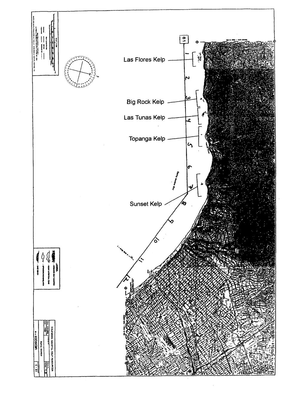
65

66

67 Kelpbedarea December31,2010 VenturaMarinaKelp:0.0047Km 2 1a

68 Kelpbedarea December31,2010 ChannelIslandHarborKelp:0.0056Km 2 1b

69 Kelpbedarea December31,2010 DeerCreekKelp:0.0620Km 2 LeoCariloKelp:0.2320Km 2 1

70 Kelpbedarea December31,2010 LeoCariloKelp:0.2320Km 2 NicolasCanyonKelp:0.2907Km 2 ElPescador&LaPiedraKelp:0.1636Km 2 2

71 Kelpbedarea December31,2010 NicolasCanyonKelp:0.2907Km 2 ElPascador&LaPierdraKelp:0.1636Km 2 LechuzaKelp:0.0959Km 2 3

72 Kelpbedarea December31,2010 PointDumeKelp:0.0938Km 2 ParadiseCoveKelp:0.2586Km 2 EscondidoWashKelp:0.2668Km 2 4

73 Kelpbedarea December31,2010 EscondidoWashKelp:0.2668Km 2 LatigoCanyonKelp:0.1423Km 2 Puerco/AmariloKelp:0.1262Km 2 5

74 Kelpbedarea December31,2010 MalibuPointKelp:0.0662Km 2 LaCostaKelp:0.0006Km 2 LasFloresKelp:0.0054Km 2 6

75 Kelpbedarea December31,2010 BigRockKelp:0.0063Km 2 LasTunasKelp:0.0147Km 2 TopangaKelp:0.0517Km 2 SunsetKelp:0.0078Km 2 7

76 Kelpbedarea December31,2010 SunsetKelp:0.0078Km 2 8

77 Kelpbedarea November4,2010 PalosVerdesKelpIV:1.1363Km 2 9

78 Kelpbedarea August22,2010 PalosVerdesKelp I:0.6204Km 2 PalosVerdesKelpI:0.2216Km 2 10

79 Kelpbedarea August22,2010 PalosVerdesKelpI:0.3886Km 2 11

80 Kelpbedarea August22,2010 PalosVerdesKelpI:0.3886Km 2 November4,2010 CabriloKelp:0.1237Km 2 December31,2010 POLA/POLBHarbor:0.2768Km 2 12

81 Kelpbedarea December31,2010 POLA/POLBHarbor:0.2768Km 2 13

82 Kelpbedarea December31,2010 POLA/POLBHarbor:0.2768Km 2 14

83 Kelpbedarea December31,2010 POLA/POLBHarbor:0.2768Km 2 15

84 Kelpbedarea December31,2010 NewportHarbor:0.0016Km 2 CoronadelMarKelp:0.1608Km 2 16

85 Kelpbedarea December31,2010 NorthLagunaBeach:0.0926Km 2 SouthLagunaBeach:0.0984Km 2 17

86 Kelpbedarea December31,2010 SouthLagunaKelp:0.0232Km 2 18

87

88 Appendix B. Explanation of historical canopy area estimations for each of the 27 CRKSC kelp beds. The earliest records are from Crandall (1912) where values for square nautical miles were converted to square kilometers. In some cases, Crandall's beds overlapped with multiple CRKSC beds. In such cases, the proportion of a historical bed occurring within a CRKSC bed was made using a digital area estimation technique to determine the appropriate percentage of the historical bed to assign to the CRKSC bed. 1 Deer Creek Does not appear in Crandall (1912) totals includes beds 1-5 Ecosystems 1989 (CDF&G 1999) 2 Leo Carillo Crandall (1912) Chart 13 - used 67% area of Bed No. 8 3 Nicolas Canyon Crandall (1912) Chart 13 - used 33% area of Bed No. 8 4 El Pescador/LaPiedra Crandall (1912) Chart 13 - used 67% area of Bed No. 7 5 Lechuza Crandall (1912) Chart 13 - used 33% area of Bed No. 7 Total 1-5 F&G 17 Crandall (1912) Chart 13 - Bed No. 7 and 8 combined = 1.21 n mi 2 = km 2 6 Pt. Dume Crandall (1912) Chart 13 - used 20% area of Bed No. 6 7 Paradise Cove Crandall (1912) Chart 13 - used 40% area of Bed No. 6 8 Escondido Wash Crandall (1912) Chart 13 - used 17% area of Bed No. 6 9 Latigo Canyon Crandall (1912) Chart 13 - used 13% area of Bed No Puerco/Amarillo Crandall (1912) Chart 13 - used 10% area of Bed No Malibu Pt. Bed does not appear in Crandall (1912) Total 6-11 F&G 16 Crandall (1912) Chart 13 - Bed No. 6 = 1.00 n mi 2 = km 2 12 La Costa Crandall (1912) Chart 13 Bed No. 5 = n mi 2 = km 2 13 Las Flores Crandall (1912) Chart 13 Bed No. 4 = n mi 2 = km 2 14 Big Rock Crandall (1912) Chart 13 Bed No. 3 = n mi 2 = km 2 15 Las Tunas Crandall (1912) Chart 13 - used 50% area of Bed No. 2 = n mi 2 = km 2 16 Topanga Crandall (1912) Chart 13 - used 50% area of Bed No. 2 = n mi 2 = km 2 17 Sunset Crandall (1912) Chart 13 Bed No. 1 = 0.28 n mi 2 = km 2 Total F&G 15 Crandall (1912) Chart 13 - Bed No. 1-5 combined = n mi 2 = km 2 18 Flat Rk-PV Pt. (IV) 19 PV Pt-PT. Vin (III) Total F&G 14 Crandall (1912) Chart 16 - combined Bed No. 24 and 20% area of Bed No. 23 = n mi 2 = km 2 20 Pt Vin to Pt Insp(II) 21 Pt Insp to Cabr (I) 22 Cabrillo Total F&G 13 Crandall (1912) Chart 16 - combined Beds No and 80% area of Bed No. 23 = n mi 2 = km 2 Total PV Crandall (1912) Chart 16 - combined Beds No = 2.53 n mi 2 = km 2 23 POLA/POLB Kelp First measured in 2005, outer harbor breakwaters only; entire harbor included in aerial surveys Horseshoe About mid-1920s (approximately stat. mi {0.25 by 0.50} width by 2.0 stat. mi length) CDF&G (Schott 1976). Disappeared by Huntington Flats Kelp bed was located offshore Huntington Beach until the 1920s in an area called the Huntington Flats. 26 Newport-Irvine Coast Crandall (1912) Bed No 20 & Fish and Game Kelp Bed No.10 Corona Del Mar - referred to as Newport or Irvine Coast includes area from Santa Ana River to Abalone Point. 27 N & S Laguna Beach Part of Fish and Game Kelp Bed No. 9 Area calculated for North Laguna Beach for 1972 and 1977 were determined by taking total area of Laguna and detemining % in north and south (WJN 1991)

89 Appendix B (Cont.). Historical canopy coverage in km² of Ventura and Los Angeles County kelp beds from 1911 to Values represent an estimate of coverage utilizing varying methods over the years. Canopy Area (km²) Kelp Bed Deer Creek ND p ND p p p p p p p p p p p p p ND ND 2 Leo Carillo p ND p p p p p p p p p p p p p ND ND 3 Nicolas Canyon p ND p p p p p p p p p p p p p ND ND 4 El Pesc/La Pied p ND p p p p p p p p p p p p p ND ND 5 Lechuza p ND p p p p p p p p p p p p p ND ND Total 1-5 (F&G 17) a ND ND ND \ ND ND ND ND 6 Pt. Dume p p p p p p p p p p p p p p p ND ND 7 Paradise Cove p p p p p p p p p p p p p p p ND ND 8 Escondido Wash p p p p p p p p p p p p p p p ND ND 9 Latigo Canyon p p p p p p p p p p p p p p p ND ND 10 Puerco/Amarillo p p p p p p p p p p p p p p p ND ND 11 Malibu Pt. ND p p p p p p p p p p p p p p p ND ND Total 6-11 (F&G 16) a ND ND ND ND ND ND 12 La Costa p ND p p p p p p p p p p p p p ND ND 13 Las Flores p ND p p p p p p p p p p p p p ND ND 14 Big Rock p ND p p p p p p p p p p p p p ND ND 15 Las Tunas p ND p p p p p p p p p p p p p ND ND 16 Topanga p ND p p p p p p p p p p p p p ND ND 17 Sunset p ND p p p p p p p p p p p p p ND ND Total (F&G 15) a ND ND ND ND ND ND ND ND ND 18 Flat Rk-PV Pt. (IV) p p ND p p p p p ND p p p p p p PV Pt-PT. Vin (III) p p ND p p p p p ND p p p p p p Total F&G ND ND ND ND ND Pt Vin to Pt Insp (II) p p ND p p p p p ND p p p p p p Pt Insp to Cabr (I) p p ND p p p p p ND p p p p p p Cabrillo ND ND ND ND ND ND ND ND ND ND ND ND ND ND ND ND Total F&G ND ND ND Total PV a a a ND b c 23 POLA-POLB Harbor ND ND ND ND ND ND ND ND ND ND ND ND ND ND ND ND ND ND 24 Horseshoe ND 1.94 d ND ND ND ND ND ND ND ND ND ND ND ND tr tr Huntington Flats ND ND ND ND ND tr Newport-Irvine Coas ND ND ND ND ND N & S Laguna Beach tr ND ND ND ND TOTAL e e e e e e ND = No Data p = this bed included in the total below tr = trace of kelp "-" = 0 a = measurement in naut m 2 converted to km 2 b = Ecoscan (1990) indicates km 2 from a July 1989 survey. Used Wilson (1989) results for PV showing the kelp beds at greatest exte c = In another survey by LACSD in 2002 total area was estimated at 2.84 k 2 d = Estimate in mid-1920s e = total is not inclusive of all beds in region Sources: Crandall (1912); 1928, 1945, 1955 from SWQCB (1964); 1955 from Neushul (1981); 1967, 1972, 1975, 1977 from Hodder and Mel (1978); Ecoscan (1990) and Wilson (1989), Veisze et al. (2004); North (2000); TMLandsat 7 (2002); MBC

90 Appendix B-1. Seasonal kelp nutritional index based on weighting values given to monthly temperature data derived from Santa Monica Pier (SMP), indicated in parenthesis, and Newport Pier (NP). The weighting values are derived from nitrate versus temperature data from North and Jones (1991), and nitrate uptake rates from Haines and Wheeler (1978), and Gerard (1982). The season begins 1 July and ends 31 June. Years in Red denote warm-water years, Blue cold-water years, both colors are transition years, based on NOAA Multivariate ENSO Index (MEI), May Number of months falling into indicated temperature range Weighting Factor Season Season Season C C C C C NQ NQ NP (SMP) NP (SMP) NP (SMP) NP (SMP) NP (SMP) NP SMP * - ( - ) 2 ( 3 ) 3( 3 ) 3 ( 1 ) 1 ( 2 ) ( - ) - ( - ) 3 ( 5 ) 3 ( 1 ) 1 ( 1 ) ( - ) - ( 1 ) 4 ( 3 ) 2 ( 2 ) 3 ( 1 ) ( - ) 2 ( 2 ) 3 ( 3 ) - ( 1 ) 1 ( 1 ) ( - ) - ( - ) 4 ( 3 ) 1 ( 2 ) - ( - ) ( 1 ) 1 ( 1 ) 3 ( 3 ) 1 ( - ) - ( 3 ) ( - ) - ( 1 ) 1 ( 2 ) 3 ( 2 ) 1 ( 2 ) ( - ) - ( 2 ) 2 ( 1 ) 2 ( 1 ) 2 ( 2 ) ( - ) 1 ( - ) 2 ( 3 ) 3 ( 4 ) 2 ( 1 ) ( - ) 1 ( 3 ) 4 ( 2 ) 1 ( 1 ) 1 ( 1 ) ( - ) 1 ( 2 ) 1 ( 3 ) 1 ( 1 ) - ( 1 ) ( - ) 2 ( 1 ) - ( 3 ) 2 ( 2 ) 3 ( 1 ) ( - ) 2 ( 4 ) - ( 1 ) 3 ( - ) - ( 2 ) ( - ) - ( - ) 1 ( - ) 1 ( 1 ) 5 ( 5 ) ( - ) 3 ( - ) 1 ( 3 ) 2 ( 2 ) 2 ( 1 ) ( - ) 3 ( - ) 1 ( 3 ) 1 ( 2 ) 2 ( - ) ( - ) 3 ( - ) 3 ( 3 ) 1 ( 4 ) - ( - ) ( - ) - ( - ) - ( 1 ) 4 ( 3 ) 2 ( 1 ) ( - ) - ( - ) - ( 1 ) 3 ( 2 ) 3 ( 2 ) ( - ) - ( - ) 3 ( 1 ) 1 ( 2 ) 2 ( 2 ) ( - ) - ( - ) 5 ( 3 ) 1 ( 3 ) 1 ( - ) ( - ) 2 ( 1 ) - ( 1 ) 2 ( 1 ) 1 ( 3 ) ( 2 ) - ( 1 ) 2 ( 1 ) 1 ( 1 ) 1 ( - ) ( - ) 1 ( 2 ) 1 ( 1 ) 4 ( 1 ) 1 ( 2 ) ( - ) - ( - ) 2 ( 3 ) 1 ( - ) 1 ( 2 ) ( - ) - ( - ) 4 ( 3 ) 1 ( 1 ) 2 ( 2 ) ( - ) 3 ( 1 ) 2 ( 3 ) 1 ( 1 ) 1 ( 2 ) ( - ) - ( - ) 1 ( 1 ) 2 ( 3 ) 2 ( 1 ) ( - ) - ( - ) - ( - ) 5 ( 1 ) 2 ( - ) ( - ) 1 ( 1 ) 3 ( 1 ) 3 ( 3 ) - ( 2 ) ( - ) - ( - ) 5 ( 1 ) 1 ( 3 ) 1 ( 1 ) ( - ) - ( - ) 4 ( 3 ) 4 ( 4 ) - ( - ) ( - ) 4 ( 3 ) 2 ( - ) - ( 2 ) - ( - ) ( - ) - ( - ) - ( - ) 2 ( 3 ) 3 ( 3 ) ( - ) 1 ( 1 ) 1 ( - ) 2 ( 3 ) 1 ( 2 ) ( - ) 4 ( 2 ) - ( 4 ) 1 ( - ) 2 ( - ) ( - ) 4 ( 4 ) 1 ( 2 ) 2 ( 1 ) 1 ( 1 ) ( 1 ) 4 ( 3 ) - ( 2 ) 2 ( 1 ) 2 ( 1 ) ( - ) - ( 3 ) 3 ( 3 ) 3 ( 1 ) 1 ( 1 ) ( 2 ) 1 ( 1 ) 3 ( 3 ) - ( - ) 1 ( 2 ) ( 2 ) 2 ( 2 ) 1 ( 2 ) 2 ( 1 ) - ( - ) ( - ) 1 ( 1 ) 2 ( 2 ) 3 ( 3 ) 1 ( 1 ) ( - ) 2 ( 3 ) 2 ( 2 ) 2 ( 1 ) 1 ( 1 ) ( - ) 1 ( 1 ) 3 ( 4 ) 2 ( 1 ) - ( - ) ( - ) 2 ( 1 ) 1 ( 3 ) 3 ( 2 ) 2 ( 1 ) ( - ) 2 ( 1 ) 1 ( 2 ) 2 ( 1 ) 2 ( 1 ) ( - ) 2 ( 3 ) 2 ( 1 ) 2 ( 1 ) 1 ( 2 ) ( - ) 2 ( 1 ) 2 ( 5 ) 2 ( - ) 2 ( 2 ) ( - ) 2 ( 3 ) 2 ( 2 ) 2 ( 2 ) 1 ( - ) ( - ) 3 ( 4 ) 2 ( 1 ) 3 ( 2 ) 1 ( 1 ) ( - ) - ( 1 ) 5 ( 4 ) 1 ( 1 ) 2 ( 2 ) ( - ) 1 ( 2 ) 2 ( 2 ) 1 ( 1 ) 1 ( 1 ) ( - ) - ( - ) - ( 1 ) 3 ( 2 ) 2 ( 3 ) ( - ) - ( - ) - ( - ) 3 ( 3 ) 3 ( 3 ) ( - ) 4 ( 2 ) 4 ( 4 ) 2 ( 1 ) 1 ( - ) ( 2 ) 2 ( 2 ) 2 ( 2 ) 2 ( 2 ) - ( - ) Totals Average * Data through 26 May 2011; 2003 and 2004 ocean temperature were measured at Kerckhoff Marine Laboratory, in Newport Harbor. Prior to 2002, all temperature data were taken from the end of the Balboa Pier, 1.1 km downcoast of the Newport Pier. Since 2002, data taken from Newport Pier and since 2010 from SCCOOS automated data from Newport Pier.

91 1911 Survey Crandall

92 1911 Survey Crandall

93 1a

94 1b

95

96 1

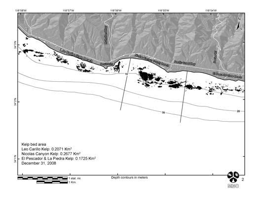
97

98 2

99

100 3

101

102 4

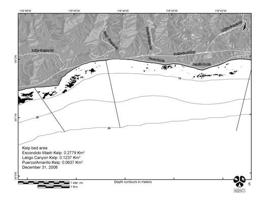
103

104 5

105

106 6

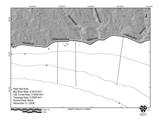
107

108 7

109

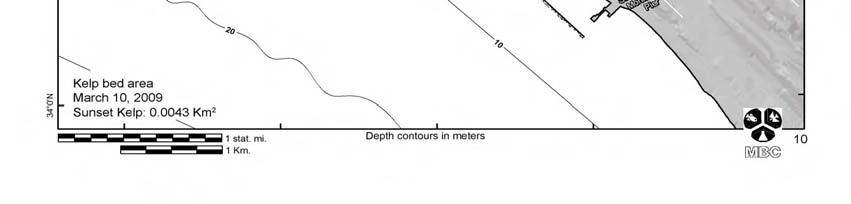
110 8

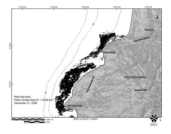
111

112 9

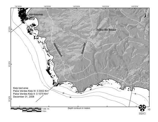
113

114 10

115

116 11

117 Palos Verdes Kelp Survey Total kelp bed area = km 2 F&G bed 14 area = km 2 F&G bed 13 area = km 2 ECOSCAN Survey Wheeler J. North

118

119

120

121

122 12

123 13

124 14

125 15

126 16

127 17

128 18

129

130

131

132

133

134

135

136

137

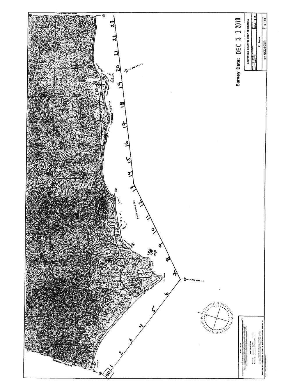
138

139

140

141

142

143

144

145

146

147

148

149

150