SPECIFIC FACTORS THAT MAY AFFECT PROFILES

Transcription

1 58 CHAPTER 4 SPECIFIC FACTORS THAT MAY AFFECT PROFILES 4.1 INTRODUCTION In reviewing the Phase I study results, the panel members raised various concerns, such as the accuracy needed for the transverse surface profiles and the effect of heavy loads, high tire pressures, or both. Additionally, the research team identified issues such as the effect of narrow shoulders. Because these issues are important to the project, they were studied with the goal of quantifying their effects and enhancing the applicability of the results. 4.2 LEVEL OF ACCURACY FOR TRANSVERSE SURFACE PROFILE MEASUREMENTS Introduction Transverse profile measurement is key to the success of the failure criteria established by this research. During the review of Phase I results, one project panel member posed the practical question of how accurate the measurement of transverse surface profiles would need to be in order to apply the types of criteria proposed by the research team. Small increments between the transverse profile measurements (e.g., less than 25 mm [1 in.]) produce more accurate profiles and, hence, more accurate distortion parameters (i.e., areas and ratios of area). However, obtaining closely spaced measurements requires additional resources, the development of new equipment, or both. In order to determine the maximum transverse measurement increment, an analysis of the error in distortion parameters was made by varying the measurement increment from 25 mm to 3 mm (1 12 in.). The profiles were compared visually to ensure that no significant loss of profile features occurred Rational Approach In addressing the issue of measurement increment for the transverse profiles, profiles from previous FEM simulations of pavement failures were used. These profiles are referred to as the original profiles. As such, distortion parameters determined from them are considered to be accurate. In other words, the parameters form the basis for comparison with distortion parameters calculated using increasingly larger transverse measurement increments. Profiles with greater transverse measurement increments were generated from the original profiles. This generation was accomplished by interpolating elevations at the desired transverse increment from the original profiles. New profiles based on the reduced data set were used to calculate the resulting distortion parameters. Figure 4-1 shows distortion parameters determined for a high-volume, large-deformation surface failure. In this figure, the values of interval from 1 to 12 correspond to the transverse measurement increment in inches. Interval refers to the original FEM-generated profiles. This FEM-generated profile used a node spacing of 25 mm (1 in.). Thus, Interval is nearly identical to Interval 1. Differences between the two are due to the horizontal node displacements that occur in the FEM mesh. Distortion parameter values become relatively constant when the transverse measurement interval is reduced to 3 in. or 4 in., regardless of failure mode Error Analysis Based on the distortion parameters determined for each transverse measurement increment from 25 mm to 3 mm (1 12 in.), the relative errors associated with the increasingly larger increments were determined. The errors were termed relative because they represented the percent difference between the distortion parameters associated with the larger increment profiles and those associated with the original profiles. The results (i.e., errors) are summarized in Tables 4-1 through 4-5; these tables are categorized by failure modes. Within the tables, column titles Err_A and Err_R represent the percent error in total area and ratio of area, respectively. Figures 4-2 through 4-6 show the error trends associated with each failure mode. The series numbers on the plots correspond to the columns in Tables 4-1 through 4-5. The data show that the surface, base, and subbase failure modes are more sensitive to the transverse measurement interval than the subgrade and heave failure modes. If an error of 1 percent is assumed to be acceptable, the critical increments for each failure mode are the following: Surface failure: Base failure: Subbase failure: Subgrade failure: Subgrade heave: 1-mm (4-in.) increment; 15-mm (6-in.) increment; 1-mm (4-in.) increment; 3-mm (12-in.) increment; and 3-mm (12-in.) increment.

2 59 TABLE 4-1 Error terms for surface failure mode TABLE 4-2 Error terms for base failure mode TABLE 4-3 Error terms for subbase failure mode

3 6 TABLE 4-4 Error terms for subgrade failure mode Note that for the base failure mode, a 178-mm (7-in.) increment actually meets the 1-percent error criteria (see Table 4-2). However, a 178-mm (7-in.) increment does not correspond to an integer number of elevation measurements for a 3.7-m (12-ft) lane width. For this reason, the original increment was replaced by the 15-mm (6-in.) increment. This 25-mm (1-in.) reduction also results in a significant reduction in error. Additionally, the data suggest that it may be possible to use an increment greater than 3 mm (12 in.) for the subgrade and heave failure modes. This statement is based on the error terms in Tables 4-4 and 4-5 being less than 1 percent and 3 percent, respectively, when 3-mm (12-in.) increments were used. However, if a 3-mm (12-in.) measurement increment were used, the specific failure mode would not be known. In order to capture any failure mode, the error analysis results suggest that a 1-mm (4-in.) transverse measurement increment should be the maximum interval used. A 5-mm (2-in.) interval is suggested for use whenever possible. There is a significant error reduction when the interval changes from 1 mm (4 in.) to 5 mm (2 in.). For example, in Table 4-1, for low-volume structures with small deformations, the error for a 1-mm (4-in.) interval is 8.95 percent, while the error for 5 mm (2 in.) is only 1.43 percent. This reduction is true for all other cases, as well, and can clearly be seen in Figures 4-2 through 4-6. The study on rut-depth measurements completed by the Texas Department of Transportation (TxDOT) using six sets of field-measured data showed that a measurement spacing of 1-mm (4-in.) increments yielded a 95-percent accuracy when compared with measurements taken at 25-mm (1-in.) spacing increments. This result agrees with the error analysis based on FEM results. TABLE 4-5 Error terms for subgrade heave failure mode

4 Visual Inspections on Profiles In order to ensure that the transverse measurement increment suggested by the error analysis did not lead to the loss of profile features, the profiles were visually inspected. This evaluation can be classified as a test of engineering reasonableness. Figures 4-7 through 4-22 show the 75-mm (3-in.), 15-mm (6-in.), and 3-mm (12-in.) increment profiles, along with the original profiles for different failure modes for both high- and low-volume structures. Figures 4-1, 4-11, 4-15, and 4-16 show that the 3-mm (12-in.) increment profiles match the original profiles quite well for the subgrade and subgrade heave failure modes. However, for the surface, base, and subbase failure modes, the 3-mm (12-in.) increment profiles do not match the original profiles, as is shown in Figures 4-7 through 4-9, 4-12 through 4-14, and 4-17 through The 15-mm (6-in.) increment profiles do appear to be acceptable for the base failure mode (see Figures 4-9, 4-14, 4-19, and 4-22). Finally, Figures 4-7, 4-8, 4-12, 4-13, 4-17, 4-18, 4-2, and 4-21 show that for the surface and base failure modes only, the 75-mm (3-in.) increment profiles match the original profiles reasonably well. The visual inspections led to the same conclusions that the error analysis did Recommendation for Measurement Increment On the basis of the previous analysis, an optimum transverse measurement increment of 75 mm (3 in.) or less and a maximum of 1 mm (4 in.) are recommended. 4.3 WHEEL PATH DISTRIBUTION Transverse Wander Wheel path distribution (i.e., wander) may be defined as the distribution of wheel loads in the transverse direction of a pavement. Several factors affect wheel path distribution, including roadway geometry, lateral clearances, traffic conditions, roadway characteristics, weather conditions, and vehicle type [55, 58 61]. Kasahara investigated the effects of wheel path distribution on estimated HMA pavement life [61]. In the investigation, a field study was conducted on Japanese highways. Video cameras were used to monitor vehicle wheel path distribution for various conditions. Pavements in the study were marked with lateral references prior to filming, and vehicle types (i.e., passenger cars and commercial vehicles) were identified from the film. Typical passenger car and commercial vehicle tire widths, wheel spacing, tire configurations, and gross weights were collected. This information was used to define wheel path distributions for several highways that had various lane widths, lateral clearances, and numbers of lanes. A three-parameter logarithmic normal distribution was found to best fit the measured wheel path distributions under each set of geometric conditions. An example comparison of measured and predicted wheel path distributions is presented in Figure In the current research, only truck loading is considered because truck traffic is by far the most important factor related to flexible pavement material and structural performance. Data from the previous study shown in Figure 4-24 indicate that wheel path distribution is a function of lane width, with wider distributions observed for wider lanes. The observed commercial vehicle wheel path (with a 95-percent confidence interval) widths for 3.7-m (12-ft) and 5.-m (16.4-ft) lane widths were 1. m (3.2 ft) and 2.2 m (7.2 ft), respectively. The effect of lateral clearance was assessed by measuring the average distance between the outer wheel path and the outer lane edge stripe. These lateral distances range from.8 m (2.6 ft) to 1.1 m (3.6 ft) on two-lane highways. The average distance between the inside of the lane edge stripe and the outer wheel path was about 1. m (3.2 ft) regardless of the shoulder width. To determine the effect of number of lanes on wheel path distribution, both two- and four-lane highways were studied. A single-lane width of 3.7 m (12 ft) was investigated. The observed wheel path distributions on four-lane pavements were slightly wider than on two-lane pavements, as shown in Figure The wheel path distributions on four-lane highways were about.15 m (.4 ft) wider. Kasahara predicted rut depths of an assumed typical pavement section with no wander (i.e., single wheel path) and distributed loading conditions. Predicted rut depths were 11 mm (.43 in.) and 3 mm (.12 in.) for the no-wander and distributed loading conditions, respectively. Buiter et al. of the Road and Hydraulic Engineering Division of the Ministry of Transportation and Public Works (in the Netherlands) investigated the effects of transverse wheel path distribution of heavy vehicles on the structural design of full-depth asphalt pavements [55]. The research included a study of the influence of lane width on the wheel path distribution of heavy goods vehicles (i.e., commercial trucks). The study was limited to determining the effect of lane width on wheel path distribution because, as stated by Buiter et al., In the literature dealing with the subject of transverse distributions of traffic loads caused by heavy-goods vehicles, it is generally concluded that the width of the traffic lane is the most significant parameter in determining the extent to which the wheel paths are distributed over the road surface. Lateral wheel path positions were measured in the right wheel path of the right traffic lane (i.e., truck lane) of 3 one-lane, 15 twolane, and 3 three-lane highways. The lanes ranged in width from 2.98 m (9.8 ft) to 3.55 m (11.6 ft). All had surfaced shoulders wider than 1.2 m (4 ft). A device was developed by the researchers to measure wheel path distributions. It was essentially a thin mat of synthetic material that could be taped to the pavement surface, which incorporated 12 switch elements, each 2 mm (.79 in.) wide. When a vehicle s tires crossed the mat, several switches were activated and the information was stored on a microcomputer. The activated switch pattern was then used to define the transverse position and width of tire(s). An example of the data generated at a site on one highway is

5 62 presented in Figure It gives the overall lateral wheel-shift pattern. The figure actually represents the number of switch movements at each contact point on the mat as a function of transverse location. Of critical importance is the standard deviation of the measured distribution identified on the figure with an S. It is clear from the figure that the distribution of wheel tracks is well represented by a normal distribution with standard deviation S. Similar data were collected for each of the 21 sites. The standard deviations were plotted as a function of lane width, and a regression analysis was conducted to define the relationship between lane width and the standard deviation of the wheel path distributions. The plot revealed that standard deviation increased as lane width increased. However, a poor regression correlation was obtained, so the data were subdivided into three lane-width classes for practical pavement design purposes. The data are presented in Table 4-6. Because of inconsistencies in reporting formats, a direct comparison of the Kasahara and Buiter et al. data could not be made. The Kasahara data are reported by confidence interval, and the Buiter et al. data are reported in terms of standard deviation. However, as the sample sizes used in these tests are all greater than 3, a normal z-distribution can be used to set up the relationship between the two sets of data. Kasahara observed a commercial vehicle wheel path width (with a 95-percent confidence interval) of 1. m (3.2 ft) for a 3.7-m (12-ft) lane width; Buiter et al. reported an average standard deviation of.29 m (.95 ft) for an average lane width of 3.5 m (11.5 ft). Plus and minus two standard deviations captures 95.5 percent of a normally distributed data set [62]. Plus and minus two times.29 m (.95 ft) is equal to a range of 1.16 m (3.8 ft), suggesting that the researchers obtained similar results. It is important to note that there is a difference in a 95-percent confidence interval and 95.5 percent of the area under a normal distribution Effect of Wheel Path Distribution on Pavement Deformation Wheel path distribution directly affects the generation of pavement distress [47, 55, 61]. As noted previously, Kasahara predicted that rutting under a no-wander condition would be about 3.5 times that which would be expected for distributed loading. Similar results were obtained from the National Pooled Fund Study (PFS) 176 [47]. In the PFS, pavement testing was conducted in the Indiana Department of Trans- portation/purdue University Accelerated Pavement Test Facility (INDOT/Purdue APT). The loading applied for the tests consisted of 4 kn (9, lb) on a standard dual-wheel configuration with 62-kPa (9-psi) tire pressure. Six APT tests were initially performed on Superpave HMA mixtures. The mixtures were compacted to two in-place density levels (low and high). Three test sections were placed at the low-density level, and three were placed at the high-density level. Two levels of wander were used for the tests: mm ( in.) (i.e., no wander) and 25 mm (1 in.). When wander was incorporated in the loading, it was randomly applied in a normally distributed fashion. Examples of the two wander cases are shown in Figures 4-27 and When loading is applied with dual wheels, singlewheel-path loading (i.e., no wander) produces significant uplift between and outside tire paths. The effect of wander is to substantially reduce (i.e., compress) uplift between the wheels and cause uplift or upheaval outside the tires to migrate away from the wheel paths. Effect of wander on rut depth is summarized in Figure In PFS tests, rutting for the single-wheel-path loading (i.e., no wander) was times that of rutting with 25 mm (1 in.) of wander. This difference is approximately one-half the ratio suggested by Kasahara s predictions Determination of Wheel Path Distribution for FEM Analysis Wheel path distribution is an important factor in determining the shape of pavement transverse profiles and, thus, distortion parameters. As indicated in the previous section, a standard normal distribution is appropriate for wheel wander, and the Buiter et al. work suggested an average standard deviation of.29 m (11.4 in.). This indication means that if wheel wander of.58 m (22.8 in.) is employed (two times the standard deviation of.29 m [11.4 in.]), 95 percent of the total wheel loads applied to a pavement will be covered. However, when the transverse wander is represented in this way for the entire duration of the loading period in a FEM simulation, the deformed mesh for the HMA failure mode shows little upheaval at the edge of the wheel paths. This result is inconsistent with the literature and field observations. A sensitivity analysis, using different transverse wander distribution widths, was conducted to evaluate the discrepancy. To determine an appropriate wander distance to be used in the finite element analysis, analysis on a high-volume structure (15 mm [6 in.] of HMA + 3 mm [12 in.] of base + 3 mm [12 in.] of subbase) was performed using wander distances TABLE 4-6 Average standard deviation by lane width classification

6 63 of.3 m,.36 m,.41 m,.46 m,.51 m, and.56 m (12 in., 14 in., 16 in., 18 in., 2 in., and 22 in.), respectively. Because surface profiles associated with HMA failure modes are more sensitive to wheel wander, the analysis was conducted for this failure mode. The resulting surface profiles corresponding to these different amounts of wheel wander are given in Figures 4-3 through Based on examination of these profiles relative to profiles found in the literature and actually observed by team members in the field,.41-m (16-in.) wheel wander was considered to be appropriate for use in further finite element analysis. Use of such a distribution in finite element analysis is a method of representing the average distribution (i.e., cumulative effect) that would occur from the initiation of rutting to the point in time when a maximum rut depth would be exhibited and the pavement would be rehabilitated. The underlying criterion for determining this distance is to use a value as close as possible to the ones given by Kasahara and Buiter et al., with the resulting surface profile conserving the same features as those from literature and field observations. This criterion can be justified because after rutting occurs, the vehicles tend to be tracked into the grooves, thus reducing the wheel wander distance. 4.4 EFFECT OF BOUNDARY CONDITIONS Figure 4-36 shows a typical pavement structure and the boundary conditions that have been employed in the FEM analysis. The selection of these boundary conditions was based on previous research conducted by team members. However, results of recent analysis led the team to question whether the constrained condition at the vertical boundary of the outside shoulder edge was appropriate. This boundary was fixed in all previous analyses because of previous research and the following considerations: All of the wheel loads that were applied to the pavement structure were confined within the 12-ft lane width, and the shoulder essentially acted as a confining structure. This boundary was 6 ft away from the pavement lane edge, so the boundary condition was not expected to have a significant effect on response of the pavement lane. After due consideration, the simplest method of justifying the fixedboundary condition at the shoulder was to perform analysis using different boundary conditions. Significance of changes in pavement response was used to determine the effect of the boundary. Extreme boundary conditions would be fixed and free, which were selected for analysis. Analysis was performed on one low-volume and two highvolume structures with the two outside-edge boundary conditions and all other conditions unchanged, as illustrated in Figure Comparisons between distortion parameters and surface profiles were made for each pair of corresponding structures. The distortion parameter results are summarized in Table 4-7, and a surface profile is shown in Figure The small differences in distortion parameters and profiles illustrate the lack of sensitivity to this boundary condition. 4.5 NARROW SHOULDER PROBLEM Shoulder width is another practical concern in FEM analysis. To expand the applicability of previous analysis on typical structures having a 1.8-m (6-ft) shoulder width (see Figure 4-36), additional analysis was performed on a pavement structure having a.6-m (2-ft) wide shoulder (see Figures 4-39 and 4-4). A 45-deg slope along the outer part of the.6-m (2-ft) shoulder was used in order to represent the weakest support condition. A free-boundary condition was assumed for the slope. A low-volume structure was chosen for the analysis because in these facility types, a narrow shoulder condition would normally exist. As shown in Figure 4-4, the structure consists of 125 mm (5 in.) of HMA and 3 mm (12 in.) of base material. This structure was used in the analysis for both HMA and base failure modes. The comparison of distortion parameters for the narrow shoulder case with a corresponding structure of 125 mm (5 in.) of HMA, 3 mm (12 in.) of base, and 1.8 m (6 ft) of shoulder is given in Table 4-8. The surface profiles are shown in Figures 4-41 through After reviewing these results, it is concluded that the results from the two cases are similar. In fact, the rut depth for the HMA failure mode is identical for both cases. The rut depth for the base failure mode is different by only.5 mm (.2 in.) for the two cases. There are slight TABLE 4-7 Comparison of FEM results for different boundary conditions

7 64 TABLE 4-8 FEM results for different shoulder widths variations in the other parameters between the two cases. However, these variations are not serious enough to dismiss the conclusion that the two shoulder cases yield the same result. 4.6 EFFECT OF HEAVY LOADS AND HIGH TIRE PRESSURE A panel member s comments raised the issue of the effect of heavier axle loads and higher tire pressures on FEM results. There was consensus among the researchers that increased axle loads and tire pressures would increase the rutting rate; however, it could not simply be assumed that the surface profiles generated for different loading conditions would be similar for a given rut depth, because the configuration of a tire footprint changes with changes in axle load and tire pressure. Therefore, analysis was performed to determine pavement response under combinations of heavy axle load and high tire pressure. The approach used to assess the effect of the combinations of heavy axle load and high tire pressure consisted of four basic steps: 1. Determine the distribution of axle loads in current traffic, 2. Determine the distribution of tire pressures in current traffic, 3. Obtain a tire footprint and contact stresses for the most commonly used truck tires under an extreme axle-loadand-tire-pressure combination, and 4. Use the new contact stresses in FEM analysis and compare the results with those obtained with the lower contact stresses employed in previous analysis. Current traffic, tire type, and axle load spectra data were obtained from the NCHRP Project 1-37A interim report, Determination of Traffic Information and Data for Pavement Structural Design and Evaluation [63]. Table 4-9 lists the most commonly used truck tires and the market share they represent. The 295/75R22.5 tire is most common, with 25 percent of the market share, while the 11R22.5 is the second most common, with 18 percent of the market share. Table 4-1 lists the tire pressures and maximum allowable load per tire for commonly used truck tires. For the purpose of finite element analysis, the tire footprint configuration and contact stresses are needed. The tire footprint and nonuniform contact stresses were available for the 11R22.5 tire, so it was selected for use in the analysis. The maximum allowable tire pressure for the 11R22.5 tire is 72 kpa (15 psi), and the maximum allowable load per tire is 26.2 kn (5,845 lb), as shown in Table 4-1. Before these data were used to obtain the corresponding tire footprint and contact stresses for modeling, the distribution of single-axle loads for trucks was investigated from weigh in motion (WIM) data summarized in the NCHRP Project 1-37A interim report [63]. The objective of this investigation was to determine if the maximum allowable load and tire pressure were similar to those reported in the interim report. The distribution of single-axle loads for each vehicle class is summarized in Figures 4-45 through Again, these data were obtained from the NCHRP Project 1-37A interim report [63]. Single-axle data were considered to be consistent with previous analysis. Figures 4-45 through 4-48 show that more than 9 percent of the axle loads observed were below 14 kn (23,4 lb), which means the load on each tire is less than 26 kn (5,845 lb) for single-axle, dual-tire usage. There- TABLE 4-9 Most commonly used tires and their market shares

8 65 TABLE 4-1 Maximum load and corresponding cold inflation pressures fore, a tire load of 26 kn (5,845 lb) with tire pressure of 72 kpa (15 psi) was selected for analysis. Figure 4-49 shows a measured tire footprint for a Goodyear 11R22.5 tire with a load of 26 kn (5,845 lb) and inflation pressure of 72 kpa (15 psi) [64]. Figure 4-5 shows the distribution of contact stresses on each of the five tire treads. The simplified tire footprint used for modeling purposes is shown in Figure As shown, each tread is replaced by a rectangle, and the contact stress on each rectangle is assumed to be constant. The load on each rectangular area sums to kn (5,838 lb), which is close to the analysis load of 26 kn (5,845 lb). Figure 4-52 shows the loading time distribution for the dual-tire single axle with wheel wander used in the finite element analysis. Both the low (2 kn per 69 kpa [4,496 lb per 1 psi]) and high (26 kn per 72 kpa [5,845 lb per 15 psi]) contact stresses were applied to two pavement structures. Two failure modes, HMA and base, were considered at the same level of rutting (25-mm [1-in.] rut depth). The pavement structures consisted of 1 mm (4 in.) of HMA on 15 mm (6 in.) of base, resting on a subgrade and 38 mm (15 in.) of HMA over 6 mm (24 in.) of base resting on the same subgrade. Figures 4-53 through 4-56 show the results of analysis (mesh surface profiles) using the high contact stresses. Figures 4-57 through 4-6 show the same for the low contact stresses on the same structures. A comparison of the distortion parameters for both contact stress levels is presented in Table After close examinations of both the profiles and distortion parameters, it can be concluded that the high contact stresses do not affect the shape of pavement transverse profile, nor do they affect the distortion parameters (i.e., total area and ratio of area) if the same rut depth is achieved. However, the contact stresses did affect the rate of rutting. In other words, the total loading time with high contact stresses to achieve a given rut depth was less than the total loading time with low contact stresses to achieve the same level of rut depth. 4.7 SUMMARY This chapter discussed in detail several factors that have the potential to affect the analysis of transverse profiles and, thus, the application of failure criteria. The first issue addressed was how accurately a transverse surface profile should be measured so that the right conclusion might be reached when applying the failure criteria. Several increments were used on profiles from the FEM analysis, and the resulting distortion parameters were compared with the theoretical ones. Using an error analysis, several maximum increments were determined to be suitable for different failure modes. HMA failure, which is the most sensitive mode to the accuracy of the transverse profiles, requires a maximum increment of 1 mm (4 in.). Because the failure mode cannot be determined before measurement of the profile, 1 mm (4 in.) is determined to be the maximum increment to be used in field measurement TABLE 4-11 Comparison of distortion parameters for different contact stress levels

9 66 in order to get reliable results. An increment of 5 mm (2 in.), which significantly reduces the errors involved in the measured profiles, is suggested for obtaining the most reliable results in field measurements. Wheel wander is another crucial issue important to the correctness of finite element analysis results. Using the work of Kasahara, Buiter et al., and PFS 176, a sensitivity analysis was performed on different wheel wander distances using finite element methods. The final wheel wander distance to be used in the FEM analysis was determined to be.4 m (16 in.), which reflects the cumulative effect of wheel wander on pavement rutting. Boundary conditions and structures with narrow shoulders were also checked, as they may also negatively affect the application of failure criteria to various kinds of pavement structures. Finite element analysis was performed, and the results were compared with those from the typical structures. In terms of distortion parameters, these factors have only minor effects and will not affect the applicability of the failure criteria. One panel member, concerned about the use of typical values for load and tire pressure, requested that the effect of using heavier axle loads and higher tire pressures be analyzed. Finite element analysis was performed using higher tire pressure and heavier axle loads, determined by the findings and observations from NCHRP Project 1-37A. The results from the FEM analysis show that higher tire pressures and heavier axle loads will not affect the pattern of the pavement surface profiles if the level of rutting is the same as that of the typical loads, though the time to achieve the same amount of rutting is reduced.

10 High Volume, Large Deformation, Surface Failure High Volume, Large Deformation, Surface Failure Total Area (in 2 ) Ratio Interval Size (in) Interval Size (in) Figure 4-1. Total area and ratio (high-volume, large-deformation surface failure). 4 Error (%) Series1 Series2 Series3 Series4 Series5 Series6 Series7 Series Transverse Measurement Increment (in) Figure 4-2. Percent of error for surface failure mode. 3 Error (%) 2 1 Series1 Series2 Series3 Series4 Series5 Series6 Series7 Series Transverse Measurement Increment (in) Figure 4-3. Percent of error for base failure mode.

11 Error (%) 4 3 Series1 Series2 Series3 Series Transverse Measurement Interval (in) Figure 4-4. Percent of error for subbase failure mode..6 Error (%).4.2 Series1 Series2 Series3 Series4 Series5 Series6 Series7 Series Transverse Measurement Increment (in) Figure 4-5. Percent of error for subgrade failure mode.

12 Series 1 Error (%) Series 2 Series 3 1 Series Transverse Measurement Increment (in) Figure 4-6. Percent of error for subgrade heave failure mode Interval Interval3 Interval6 Interval12 Figure 4-7. Profiles for high-volume, large-deformation surface failure Interval Interval3 Interval6 Interval12 Figure 4-8. Profiles for high-volume, large-deformation base failure.

13 7.4.2 Interval Interval3 Interval6 Interval Figure 4-9. Profiles for high-volume, large-deformation subbase failure..4.2 Interval Interval3 Interval6 Interval Figure 4-1. Profiles for high-volume, large-deformation subgrade failure. Interval Interval3 1.2 Interval6 Interval Figure Profiles for high-volume, large-deformation subgrade heave Interval Interval3 Interval6 -.2 Interval Figure Profiles for high-volume, small-deformation surface failure.

14 Interval -.1 Interval3 -.2 Interval6 Interval Figure Profiles for high-volume, small-deformation base failure Interval -.2 Interval3 Interval6 -.3 Interval12 Figure Profiles for high-volume, small-deformation subbase failure Interval Interva3 Interval6 Interval12 Figure Profiles for high-volume, small-deformation subgrade failure..4.3 Interval Interval3 Interval6 Interval Figure Profiles for high-volume, small-deformation subgrade heave.

15 Interval Interval3 Interval6 Interval12 Figure Profiles for low-volume, large-deformation surface failure Figure Profiles for low-volume, large-deformation base failure. Interval Interval3 Interval6 Interval Interval Interval3 Interval6 Interval12 Figure Profiles for low-volume, large-deformation subgrade failure Interval -.2 Interval3 Interval6 -.3 Interval12 Figure 4-2. Profiles for low-volume, small-deformation surface failure.

16 Interval -.2 Interval3 Interval6 -.3 Interval12 Figure Profiles for low-volume, small-deformation base failure Interval -.2 Interval3 Interval6 -.3 Interval12 Figure Profiles for low-volume, small-deformation subgrade failure. Figure Observed and estimated wheel path distributions [4].

17 74 Figure Influence of lane width on wheel path distribution [4]. Figure Influence of number of lanes on wheel path distribution [4].

18 75 Figure Example measured lateral wheel-shift pattern [5]. Predicted Cross Section of APT Lane (44 Below, Low Density) Cross Section Profile, mm wander=26 mm. wander=13 mm. wander=. mm Offset Distance, mm Figure Wander effect on transverse surface profile for PFS 176 low-density mixture.

19 76 Predicted Cross Section of APT Lane (44 Below, High density) Cross Section Profile, mm wander=26 mm. wander=13 mm. wander=. mm Offset Distance, mm Figure Wander effect on transverse surface profile for PFS 176 high-density mixture [6]. Rut depth Vs. Wander (44 Below) 12 1 low density high density 8 Rut Depth, mm Wander, mm Figure Wander effect on rut depth on PFS 176 [6].

20 77 Figure 4-3. Surface profile for 3-mm wander. Figure Surface profile for 35-mm wander. Figure Surface profile for 4-mm wander. Figure Surface profile for 45-mm wander. Figure Surface profile for 5-mm wander. Figure Surface profile for 55-mm wander.

21 78 HMA Shoulder Base Symmetry Line Subgrade Figure Structures with vertical boundary constrained along shoulder. HMA Shoulder Base Symmetry Line Subgrade Figure Structures with vertical boundary free along shoulder.

22 79 Figure HMA failure for structure with constrained shoulder, 75 mm HMA + 3 mm base. Figure Boundary conditions of pavement with 6-mm shoulder.

23 8 Figure 4-4. Structural geometry of pavement with 6-mm shoulder. Figure HMA failure, 1,8-mm shoulder.

24 81 Figure HMA failure, 6-mm shoulder. Figure Base failure, 1,8-mm shoulder.

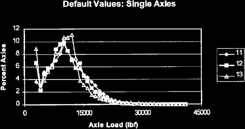
25 82 Figure Base failure, 6-mm shoulder. Figure Distribution of axle loads for Vehicle Class 4. Figure Distribution of axle loads for Vehicle Classes 8, 9, and 1. Figure Distribution of axle loads for Vehicle Classes 5, 6, and 7. Figure Distribution of axle loads for Vehicle Classes 11, 12, and 13.

26 83 Figure Tire footprint of Goodyear 11R22.5 (load = 26 kn, tire pressure = 72 kpa). 1 8 Contact Stress (kpa) Test Pin Figure 4-5. Contact stress distribution for Goodyear 11R22.5 (load = 26 kn, tire pressure = 72 kpa).

27 kpa kpa kpa kpa kpa Geometry Unit: mm Figure Simplified tire footprint (load = 26 kn, tire pressure = 72 kpa). Figure Distribution of loading time for dual tires (Goodyear 11R22.5).

28 85 Figure HMA failure under high contact stresses, 1 mm HMA + 15 mm base. Figure Base failure under high contact stresses, 1 mm HMA + 15 mm base.

29 86 Figure HMA failure under high contact stresses, 375 mm HMA + 6 mm base. Figure Base failure under high contact stresses, 375 mm HMA + 6 mm base.

30 87 Figure HMA failure under low contact stresses, 1 mm HMA + 15 mm base. Figure Base failure under high contact stresses, 1 mm HMA + 15 mm base.

31 88 Figure HMA failure under low contact stresses, 375 mm HMA + 6 mm base. Figure 4-6. Base failure under high contact stresses, 375 mm HMA + 6 mm base.

32 89 CHAPTER 5 DEVELOPMENT OF TOOLS FOR DATA EVALUATION AND NEW CRITERIA 5.1 INTRODUCTION Using the theoretical analysis of different pavement failure modes, the previously developed criteria can be further refined. Chapter 4 resolved some practical issues concerning the results of finite element analysis, and the results did not indicate any significant adverse effects on the general findings from the finite element analysis. This chapter describes a program used to prepare finite element data and to calculate distortion parameters. The problem associated with the initial criteria is then explained, and more specific criteria are developed using the basic concept of the initial criteria and the distortion parameters calculated from finite element analysis. To facilitate the use of the new criteria, an input table and a failure chart are developed using spreadsheet software. Detailed guidance on how to use the table and chart is given after the new criteria are introduced. 5.2 DEVELOPING THE PAVEMENT ANALYSIS ASSISTANT PROGRAM Initiative and Objective The research team developed a program called Pavement Analysis Assistant Program (PAAP) in December The first reason for developing the program was to ease the preparation of finite element analysis data. After the matrix of finite element analysis was constructed, it was estimated that it would take at least 378 finite element runs to get the desired results. Displacement was used as the control factor in order to achieve a small deformation (5 8 mm [.2.31 in.]) and a large deformation (22 25 mm [ in.]) for each pavement structure. Because different structures require different loading times to achieve equivalent levels of deformation, the amount of work in preparing the loading data for just uniform contact stress and no wheel wander distribution was enormous. Given also the total amount of time needed for finite element calculations, the theoretical analysis could not be finished on time unless the process of data preparation could be accelerated. The second reason for developing the program came from a requirement of the research team to perform the simulation using dual-tire configuration, nonuniform contact stress, and wheel wander distribution. The incorporation of these factors made it impossible to prepare the load data for 378 finite element runs by hand calculation and get the correct load data. It was imperative to develop a computer program to perform these tedious tasks, not only for convenience, but also for accuracy. Finally, the results from finite element analysis are in the form of node displacement. To calculate the distortion parameters (i.e., total area and ratio of area), a tremendous amount of calculation must be completed. The pavement-structure cross slope made hand calculations even more difficult, which motivated the research team to use PAAP to extract data directly from the finite element results, specifically from ABAQUS output files, and to calculate all the distortion parameters. With these needs in mind, PAAP was designed to generate the loading data for ABAQUS input files using dual-tire configuration, nonuniform contact stress, and wheel wander distribution. When the finite element analysis is done, PAAP is able to extract the surface profile from the ABAQUS output file and calculate all the distortion parameters Functionalities of PAAP PAAP was developed using the Java programming language and can be run in many operating systems, such as Windows 95/98/NT/2, Linux, and Solaris V. The advantage of using Java is that Java runs on a platform called the Java Virtual Machine (JVM) and, thus, the program itself is independent of the operating system. PAAP is packaged such that it can run on Windows 95/98/NT/2 directly (the JVM is included in the package). On Unix systems, such as Solaris V, the Java SDK 1.17 or higher together with Swing utility have to be installed before PAAP can be used. The functionalities of PAAP are roughly divided into two parts: preprocessing for generating load data and postprocessing for calculating distortion parameters PAAP Preprocessing To establish loading data for ABAQUS using PAAP, two set-up files are needed: nodeinfo.txt and *.cfg ( * can be any valid filename). The nodeinfo file stores the FEM pavement surface (typically 3.7-m [12-ft]) node information, where

33 9 the load is applied and the profile is retrieved. The *.cfg file provides the wheel configuration that will be used to generate loading data. The nodeinfo.txt file name should never be changed because PAAP implicitly looks for this file when running; the file content can be changed as long as it conforms to the following format: num N1 N2 N N 3 X1 X2 X3... X Y1 Y2 Y Y num num num where num = the total number of surface nodes within the 3.7-m (12-ft) lane, including both end points; N 1 = the node number in the finite element model; and X 1, Y 1 = coordinates of N 1 on the original structure. The following lines from N 2 through N num have the same meaning. This information can be extracted from the ABAQUS input file named *.inp when the finite element model has been set up. The reason for using the.cfg configuration file is to make PAAP flexible in supporting different types of axle configurations (single or dual tire), tire footprints, and contact stresses. PAAP offers two sample files named wheel1.cfg and wheel2.cfg. The former is for a dual tire with an 8-kN (18,-lb) axle load and 62-kPa (9-psi) tire pressure; the latter is for a single tire with an 8-kN (18,-lb) axle load and 62-kPa (9-psi) tire pressure. The following shows a sample wheel1.cfg file, which is used to illustrate the configuration file format. It is assumed that the two sets of tire(s) on an axle are identical so that only one set of data is needed; the other set is generated automatically by PAAP. UNIT DIST n a1, b1, F1, P1 a2, b2... F2, P2 a, b F, P n n n n 3 where UNIT = either mm or inch indicating the units used in this file, DIST = distance from the tire center to the center of the axle, n = total number of rectangles used to simulate the tire footprint in one set of tire(s) (on one side of an axle), a n, b n = relative horizontal positions of the rectangles to the tire center (see Figures 5-1 and 5-2), F n = length factor for a rectangle, which is used for distributing loading time, and P n = contact stress on the nth rectangle (bounded by a n and b n ). The definition of DIST for single- and dual-tire configurations is illustrated in Figures 5-1 and 5-2, respectively. For the same number of wheel passes, rectangles with different lengths have different pavement loading durations. The maximum length of all the rectangles is given as a factor of 1. All other length factors are calculated by simply taking the ratio of any given rectangle length to the maximum rectangle length. It should be noted that all the rectangles in a wheel configuration file may be uniquely defined; that is, no symmetric condition is imposed. For example, the two tires on one side of the axle in the dual-tire configuration need not be identical, though in most situations they are set so as to be symmetric. This gives PAAP more flexibility in generating data for different tire conditions that may be encountered in practice. When the two configuration files are completed, PAAP can be used to generate the loading data for ABAQUS. Again, the loading data correspond to the nodes defined in the file nodeinfo.txt. If data for a different structure are to be generated, this file must be modified first. After execution, PAAP displays a window interface, as shown in Figure 5-3. To use the load-generating function, the user must select Loading Time from the Plot pull-down menu or click the rightmost button on the tool bar (see Figure 5-4). A file selection window is then displayed for selecting the wheel configuration file (see Figure 5-5). After a *.cfg file is chosen, PAAP will show the loading time and tire configuration default values for a total loading time of 2, s and a.4-m (16-in.) wheel wander distribution (see Figure 5-6). Descriptions of the items listed in the right panel are as follows: (1) FEM Data Information in this box cannot be changed directly. It is extracted from the two configuration files and listed here for verification: Node No: Number of nodes on the surface from the finite element model. Step No: Number of steps to be used in the ABAQUS analysis. This number is actually the number of levels of contact stresses used in the wheel configuration file. Data Unit: (2) Control Data: Axle Center: Units used in the wheel configuration file (i.e., inch or mm). The relative distance of the axle center from the left side of the pavement. The default value is 1.8 m (72 in.), which means the axle center is the same as the lane center. This value can be changed in order to shift the load on the pavement surface if so desired.

34 91 Wander: Total Time: Wheel wander distance used in the finite element analysis. This number must have the same units as indicated in the wheel configuration file. Total time to be distributed according to the wander distribution pattern. After setting the values in the data control box, the data can be generated and saved in a text file. The command for this operation is Export from the File pull-down menu or the forth button from the left on the tool bar (see Figure 5-7). In the file selection window, simply type in a file name and the data are saved in an ABAQUS-formatted file PAAP Postprocessing When the ABAQUS finite element analysis is completed, the profile data can be extracted from the ABAQUS output file (*.dat) using PAAP. To do this extraction, the user first selects Profile in the Plot pull-down menu or clicks the sixth button from the left on the tool bar to switch to the postprocessing capabilities. The Import function from the File menu (see Figure 5-8) is then selected to choose a data file. This selection can also be accomplished by using the Import button (third button from the left) on the tool bar. Select the desired data (*.dat) file when the File Selection pop-up menu is opened (see Figure 5-9) and click on Open. PAAP will then display the surface profile in the left blank area and all the distortion parameters on the right panel (see Figure 5-1). Descriptions of the items listed in the right panel are as follows: (1) Results: Difference: Rut Depth: Above Area: Below Area: Total Area: Ratio (A/B): (2) Unit: Data: Display: The maximum difference in the Y coordinates after the cross slope is removed. The maximum rut depth determined by the wire method. (See Figure 3-8 in Chapter 3 for an illustration of the wire method.) Areas above the horizontal line, also called Positive Areas. Areas below the horizontal line, also called Negative Areas. The sum of Above and Below areas. The ratio of Above and Below areas in absolute value. The units used in the ABAQUS input files or the profile data files. May be either mm or inch. The preferred units for displaying the results in the Results box. May be either mm or inch. (3) Drawing Scale: Scale_Y: The factor for scaling profile Y coordinates. Mostly used to scale profiles up. The default value is 1. Figure 5-11 shows a profile with a scale of 5. There are two selections in the Option pull-down menu that are specifically used for drawing profiles, Fill Areas and Show Wires (see Figure 5-12). The first shows the areas in shaded pattern (see Figure 5-13), while the second shows the wires on the profile (see Figure 5-14). The PAAP format to store a profile file is quite simple in PAAP; it makes PAAP capable of reading from handgenerated profiles and calculating the distortion parameters. In fact, all the field data profiles were processed by PAAP in order to get the distortion parameters. The file for storing a profile is a plain text file named *.prf and has the following format: n X X X... X n Y Y Y Y n total number of points in the file coordinates of the first point coordinates of the secont point coordinates of the third point coordinates of the last point If the data are measured over pavement surface that has a cross slope, PAAP will automatically remove the cross slope before it calculates the distortion parameters. To open a hand-generated file for profile data or an existing profile file generated by PAAP, use the selection Open in the File pull-down menu. By default, PAAP will seek files with the extension.prf. 5.3 DEVELOPING NEW CRITERIA FROM FEM RESULTS Review of Initial Failure Criteria The initial layer failure criteria (see Table 2-9) were used throughout the FEM analysis. The basic concept of the criteria is that pavement layer failure may be distinguished by certain characteristics of the surface transverse profile for example, the total or absolute area and ratio of area computed from the rutting depression (negative area) and uplift (positive area) of the profile. There is a potential problem with the initial criteria in that the parameters are not associated with rut depth. For example, consider the case of a base failure that occurs in conjunction with a small rutting level. The total area calculated for such a failure would indicate an HMA failure even though it would not be the case. Nevertheless, the initial criteria were developed before the theoretical analysis was completed, and, thus, the basic concepts were applied in developing the refined criteria.

35 Review of Results from Finite Element Analysis Intensive finite element analysis was performed on a matrix of different pavement structures, and the results are summarized in Chapter 3. The characteristics of each failure mode can now be examined in terms of the maximum rut depth and total areas. Differentiation between low-volume and high-volume structures is not necessary because the results are to be generalized for application to any pavement structures. The relationships of total areas versus maximum rut depth for all the finite element models are shown in Figure 5-15, with two deformation levels: small and large. Figure 5-15 shows that the total areas for the same failure tend to cluster at the same rutting level. This tendency is true for both small and large deformations. The difference between area clusters increases as the deformation increases. Examination of the data also indicates that the total areas for dividing two failure modes are a function of rut depth. For example, at a rut depth of 6 mm (.24 in.), the total area for an HMA failure should be greater than 8, mm 2 ( 12.4 in. 2 ). For a base failure, the total area should be less than 8, mm 2 ( 12.4 in. 2 ). However, at a rut depth of 25 mm (1 in.), the total area for an HMA failure should be greater than 28, mm 2 ( 43.4 in. 2 ), while it should be less than 28, mm 2 ( 43.4 in. 2 ) for a base failure. This overlapping in total areas for different failure mechanisms at different rutting levels suggests that rut depth can be used as a component of the failure criteria. Average values of total area for the two levels of rutting were determined for the different failure modes. The three trend lines are shown in Figure These trend lines accentuate the differences in the values of total area for the larger rut depth Criteria Revision The acceptance of failure criteria depends on accuracy and simplicity. For example, in Figure 5-15 the difference in total areas for the same failure modes varies with thickness. However, layer thickness is not considered as a factor in the criteria for two reasons: In practice, accurate layer thickness will not be known. Sometimes even approximate numbers are not available. Pavements may have different combinations of layers and thickness. It is not possible to develop simple criteria with all possible combinations. With this philosophy in mind, the approach used to develop the suggested criteria can be explained using Figure Lines midway between the trend lines in Figure 5-16 will be used as criteria to differentiate failure mode. These lines are transparent criteria and can be adjusted if field data indicate that it is necessary. For example, the research team initially set the line dividing HMA failure and base failure midway between the trend lines for these two failure modes. If the research team has field data that, in this failure chart, are slightly below the midway-line, the failure may be classified as a base failure using the criteria. But if field observation indicates that the failure is an HMA failure, the research team has to move the midway-line slightly down so that the data point will appear above the line and denote an HMA failure. There are two things to be noted. First, the adjustment should be done during the validation of criteria, not during the application of the criteria to determine failure. Second, the adjustment usually is made when failure occurs mainly in one layer but when there exists certain contribution (though small) from the other layer. This adjustment can usually be made by checking the ratio of area, as in the case in Ohio SPS-8 data. So the adjustment of midway-lines is not expected to happen often. It can be seen from the definitions of ratio of area and total area that the more negative area there is, the smaller the total area and ratio of area. If only one of the two parameters, either total area or ratio of area, could be used to identify failure, the criteria might be simplified. Unfortunately, this possibility has been investigated and found to be unrealistic. The total area is needed to differentiate between base and subgrade failures because finite element analysis indicates that the ratio of area is zero for all subgrade failures and most base failures. However, total area itself is not sufficient to distinguish between HMA and base failures. For example, when a pavement shows base failure but there is a certain (though small) amount of contribution from HMA layer, the total area parameter may indicate HMA failure. The trenching data from Ohio SPS-8 Site 3911, Station 4-, clearly demonstrate this case (details of this site are given in Chapter 6). By checking the results from finite element analysis, it was found that the ratios of area for all base failures were less than.5. Because the structures used in finite element analysis covered a wide range of pavement structures, it is reasonable to claim that it cannot be an HMA failure if the ratio of area is less than.5, though that number may be adjusted if field data indicate the necessity. The recommended procedure for determining which failure mode has occurred in a pavement structure is as follows (see Figure 5-17): For area ratios greater than or equal to.5: If the total area is above a line midway between the average lines of HMA and base (see Figure 5-16) and the profile shows a curvature reversal in the middle, then the failure occurred in the HMA layer; otherwise, it is a base failure. For area ratios less than.5: If the total area is above a line midway between the average base and subgrade lines, then the failure is in the base; otherwise, the failure is in subgrade. The rationale for using the total area and curvature reversal to distinguish between HMA and base failure, when the area ratio is greater than.5, is based on the following concern.

36 93 For some pavement structures, there exists a crown at the lane center in addition to the crown built in the middle of two lanes. This type of construction results in a hump in the middle of the measured profiles. Field data from MnROAD show profiles with this hump, and it was confirmed that these pavement sections have a crown built at lane center (see Chapter 6). Thus, there is the possibility for a base failure with a ratio of area greater than Development of a Criteria Input Table and Failure Chart To simplify the process of determining pavement failure, an input table called Failure Identification Table (FIT) was devised using spreadsheet software; the software hides all of the details involved (see Table 5-1). Each horizontal record in the table corresponds to one profile and has eight columns, with the first five columns for input and the last three for output. The first two columns are for recording the locations where the data were obtained (text data). The third to fifth columns are for input of the three distortion parameters: rut depth, total areas, and ratio of area. These three parameters can be obtained from PAAP, as described previously. Once the data are put into the table, the failure mode can be determined and the result will be shown in one of the last three columns. For example, the first row in Table 5-1 shows an HMA failure, while the sixth row shows a base failure. The input table is preformatted and ready for direct use. The result from Table 5-1 will automatically be displayed in the failure chart shown in Figure Figure 5-18 is the failure chart with the results from Table Variance Analysis of Trend Lines The trend lines in the failure chart were developed using the results of finite element analysis. Although data points tend to cluster for each failure mode, there exist variances among the pavement structures used in the finite element analysis. It can be seen from Figure 5-18 that all three trends pass nearly through the origin; thus, a variance analysis of slopes can show differences in the slopes of the trend lines. The slopes were calculated for each of the paired data points having identical conditions (e.g., cross section and shoulder type) except for their rutting level (i.e., small and large). The slopes for the three failure modes (HMA, base, and subgrade) are given in Table 5-2. Average slopes and standard deviations for each failure are then calculated separately and are also shown in Table 5-2. Confidence intervals of the slopes can be calculated as follows: T s ± t 1 α 2 ( 51 - ) n where T = average slope, t = the t-distribution, α=confidence level, s = standard deviation, and n = number of data points used in calculating the average. The 9-percent, 95-percent, and 99-percent confidence intervals of the average slopes for each failure mode are listed in Table 5-3. There is no overlapping of the confidence intervals, and, thus, the failures are distinguishable by the trend lines. For example, the 99-percent confidence intervals for HMA, base, and subgrade failures are ( 958, 76), ( 1,643, 1,336), and ( 2,317, 1,974), respectively. 5.4 SUMMARY More specific criteria for delineating failure modes were developed using concepts applied in determining the initial criteria and results from finite element analysis. The approach was to develop practical criteria that can be easily applied. Spreadsheet software was used to develop a failure criteria chart, as well as a data input table. TABLE 5-1 Input table for using pavement failure criteria

37 94 TABLE 5-2 Average trend line slopes and their standard deviations by failure mode TABLE 5-3 Confidence intervals of the trend line slopes for each failure

38 95 Tire Center DIST Axle Center a1 b1 a5 b5 a2 b2 a4 b4 a3 b3 Figure 5-1. Single-tire configuration with five rectangles. Tire Center DIST Axle Center a1 b1 a5 b5 a2 b2 a4 b4 a3 b3 a6 b6 a1 b1 a7 b7 a9 b9 a8 b8 Figure 5-2. Dual-tire configuration with 1 rectangles.

39 96 Figure 5-3. Starting window interface of PAAP. Figure 5-4. Menu of selecting load generation function.

40 97 Figure 5-5. Selection window for wheel configuration file. Figure 5-6. Loading time and tire configuration for a dual-tire axle.

41 98 Figure 5-7. Generating the loading data for ABAQUS. Figure 5-8. Import profile data from ABAQUS output files.

42 99 Figure 5-9. Choose an ABAQUS output file with extension.dat. Figure 5-1. An example profile drawn by PAAP.

43 1 Figure Profile drawn with a large scale. Figure Assisting functions for plotting profiles.