The influence of dredging activities on the morphological development of the Columbia River mouth MSc Thesis

Transcription

1 The influence of dredging activities on the morphological development of the Columbia River MSc Thesis Jeroen Stark Deltares, 2012

2

3 Title Pages 145 Keywords Long-term morphodynamics, Columbia River, ebb-tidal delta, jetty construction, dredging activities, fluvial sediment supply, Delft3D modelling, morphological acceleration techniques Abstract This is a numerical modelling study on the impact of dredging and disposal activities on the long-term morphological development of the Columbia River (MCR). Dredging activities removed 120 Mm 3 of sand from the MCR during the studied interval between 1958 and Only one-third of this volume was disposed in the active littoral zone. Therefore, dredging activities might be an important factor for recent erosion trend at the coasts directly adjacent to the MCR. The net influence of both dredging and disposal activities is analyzed by making use of a Delft3D model. Morphological acceleration techniques and wave climate reduction are used to bridge the gap between hydrodynamic and morphological time scales. The model performance is assessed with simulations for the interval. These simulations indicate that the model captures the large-scale morphological changes that occurred in the study area. Simulations for the interval are then used for the analysis of the impact of dredging and disposal activities. Based on the model results, dredging activities led to significant volume losses in the inlet itself and in the area west of the river entrance. On the Peacock Spit shoal directly north of the inlet, the volume losses due to dredging are almost completely reversed by disposal of dredged material on the shoal itself. Dredging and disposal activities did not have significant effects for the littoral drift at coastal stretches adjacent to the MCR. In the studied period, the Peacock Spit shoal did absorb the negative effects of dredging and the additional supply due to disposal activities, without reducing its sediment supply function to the adjacent coastal cell. Other effects of dredging and disposal activities were the formation of distinct sand mounds at the locations of some disposal sites and maintaining the southern orientation of the MCR channel at the estuary side of the inlet. Main implication of the model results for disposal strategies is that the sand volume of the Peacock Spit shoal should be maintained to avoid further erosion of the shoal and prevent undermining of the North Jetty and to maintain the sediment supply function of the shoal for the updrift coastal cell. Graduation committee prof. dr. ir. M.J.F. Stive ir. A.P. Luijendijk ir. D.J.R. Walstra dr. ir. E. Elias dr. G. Gelfenbaum dr. ir. J.E.A. Storms (TU Delft) (Deltares / TU Delft) (Deltares / TU Delft) (Deltares) (USGS) (TU Delft) Version Date Author Initials Review Initials Approval Initials june 2012 Jeroen Stark JS State final

4 04 July 2012, draft

5 04 July 2012, draft The influence of dredging activities on the morphological development of the Columbia River Master of Science Thesis by Jeroen Stark June 2012 Thesis submitted to obtain the degree of Master of Science in Civil Engineering at Delft University of Technology Department of Hydraulic Engineering Section of Coastal Engineering

6 04 July 2012, draft

7 04 July 2012, draft Summary This is a Delft3D modeling study about the impact of dredging and disposal activities on the large-scale morphological changes at the Columbia River (MCR). Jetty construction in the late 19 th century significantly disturbed the dynamic equilibrium situation of the entire coastal system near the MCR. Together with a suspected reduction in sediment supply from the Columbia River, it caused an ongoing evolution of the MCR and adjacent coasts. Confined ebb-flows through the narrowed river entrance pushed large amounts of sediment from the former ebb-tidal deltas into deeper water. The nearshore flanks of the delta initially dispersed onshore and then alongshore away from the MCR, causing adjacent shorelines to accrete at much higher rates than before jetty construction. Over time, the accretion rates of the beaches directly adjacent to the jetties decreased or even reversed to rapid erosion. Apparently, the sediment supply from the former shallow ebb-tidal deltas and from the Columbia River did decrease. Dredging of the MCR navigation channel is an important cause for the decreased sediment supply from the Columbia River estuary to the littoral cell. Approximately 120 Mm 3 of sediment was removed from this channel during the studied interval between 1958 and Only one-third of the total dredged material was placed at the nearshore disposal site on the Peacock Spit shoal west of the North Jetty. The remaining two-third was dumped at offshore disposal sites and is largely lost for the littoral system. This study assesses the influence of dredging activities and disposal of dredged material on the long-term morphological development of the MCR. Special attention is paid to the impact of dredging activities on the sand volume of the Peacock Spit shoal and the sediment feeding function of this shoal for the updrift Long Beach coastline. Delft3D model of the MCR The Delft3D model that is used in this study was constructed by Elias and Gelfenbaum (2009) and adapted for long-term morphological modeling by Moerman (2011). State of the art morphological acceleration techniques are used to reduce computation times for long-term model simulations. These techniques include the application of a morphological tide (Lesser, 2009) and wave climate reduction with the Energy Flux method (Dobrochinsky, 2009) and the Opti-routine (Mol, 2007). A constant amplification factor is applied in the schematization of the morphological tide. This schematization is not mathematically founded for situations where the interaction of tidal flow with density-driven circulation is of significant importance for the residual transport such as the MCR. Finally, variable morphological acceleration factors are used to effectively bridge the gap between hydrodynamic and morphological time scales. In this study, several improvements are made with respect to the model schematization. A new reduced wave and discharge climate is developed to obtain a more accurate representation of the alongshore transports. Historical dredging and disposal activities for the interval are schematized and implemented in the model simulations. Besides, the bed schematization of the estuary sub-domain is altered for the simulations so that the model better reproduces the net sediment supply from the estuary towards the littoral cell. Model simulations are performed for two time intervals: (Period B) and (Period C). The Period B simulations are used to analyze the model performance by comparing the model results with observed morphological changes, both qualitatively as well as quantitatively. After implementing the dredging and disposal activities for Period C, the

8 04 July 2012, draft model was successfully used to analyze the impact of these activities on the large-scale morphological development of the MCR. The MCR model does reproduce the large-scale morphological changes that occurred in the study area. Quantitatively, the volumetric changes at the MCR are represented with an accuracy ranging from only 2% to a local maximum of about 50%. Some limitations and deficiencies do however apply to the MCR model. The representation of morphological features such as the Peacock Spit shoal and the part of the MCR channel between the entrance jetties is slightly different from the observed bathymetries. Peacock Spit flattens out and expands too far to the north in all model simulations and the MCR channel is represented too wide, causing the western part of the Clatsop Spit shoal to erode. From a visual analysis of the Period C simulation results, it appears that the model underestimates the shoreline advance in the Long Beach coastal cell. Furthermore, the model results appear to be very sensitive to the applied bed schematization, which is done simple and only consists of two sediment fractions. The impact of dredging and disposal activities Simulations for are performed without dredging activities, with only dredging implemented and with both dredging and disposal activities included. The net influence of dredging and disposal activities on the MCR morphology and on the littoral drift in adjacent coastal cells is assessed by comparing these model simulations. Dredging activities induced significant net volume losses west of the river entrance and in the inlet itself because the sediment input from the Columbia River estuary decreased. In addition to that, dredging activities at the estuary side of the inlet maintained the southern orientation of the channel and prevented the Clatsop Spit shoal from expanding to the north. Distinct sand mounds in the surrounding bathymetry formed at disposal sites A, B and to a lesser extent F. On the Peacock Spit shoal, dredging activities between 1958 and 1999 induced a net volume loss of approximately 33 Mm 3, based on the model results. However, disposal of 43.5 Mm 3 of material at placement site E during Period C did increase the sand volume of the shoal by 31 Mm 3. The negative effect of dredging was thus almost completely reversed by disposal activities at Site. It should however be stated that the model underestimates impact of dredging activities by about 20%, as only 97 Mm 3 of the total 120 Mm 3 of dredged material is removed in the model simulations. In the studied period, the littoral drift north of Peacock Spit in the Long Beach sub-cell was not affected by dredging and disposal activities in the MCR. The shoal absorbed the sediment losses due to dredging and the accumulation due to disposal activities, without significant changes to its sediment supply function for the updrift coastal cell. Main implication of the model results for disposal strategies is that depletion of Peacock Spit should be counteracted by continuing disposal of sand at the disposal site on the shoal. Undermining of the North Jetty is prevented this way and the sand supply function of the shoal towards the adjacent coast can be maintained. Sediment supply from Peacock Spit to the adjacent coast depends on the sand volume and the shape of the shoal, which could be harmed if there is not enough dredged material placed on the shoal in the future.

9 04 July 2012, draft Acknowledgements This thesis is written to finalize my Master of Science program in Hydraulic Engineering at the Faculty of Civil Engineering and Geosciences, Delft University of Technology. The study was conducted at Deltares in Delft and at the United States Geological Survey (USGS) in Santa Cruz, California. In general, I would like to thank Deltares and the USGS Pacific Coastal and Marine Science Center in Santa Cruz for making it possible to carry out my graduation project at their offices. My gratitude goes to the graduation committee for their supervision and guidance during the entire project. I would like to thank ir. A.P. Luijendijk for providing me with the thesis subject, for his daily supervision at Deltares and for his advice and help with the Delft3D model; dr. ir. E. Elias for sharing his knowledge on the subject and for his critical approach on the model results and the thesis itself; ir. D.J.R. Walstra for his comments and enthusiastic approach; and dr. ir. J.E.A. Storms and prof. dr. ir. M.J.F. Stive for their input during the committee meetings. Greatest gratitude goes to dr. G. Gelfenbaum for helping me during my stay at the USGS, for providing me with interesting articles and additional input and for making my stay in the United States even more enjoyable. Furthermore, I would like to thank the fellow students and colleagues at Deltares and the USGS for their help, discussions and nice talks at work, lunch and coffee breaks, especially Andrew Stevens for lending me a bike during my stay in Santa Cruz. Finally, I want to thank my parents for their unconditional support during my entire study. Jeroen Stark Rotterdam, June 2012

10

11 Contents List of Tables List of Figures iv v 1 Introduction Study Area Columbia River littoral cell Columbia River Mouth of the Columbia River Morphological change in the MCR Problem description Literature review Sediment budget studies on the Columbia River littoral cell Modeling studies on the MCR Research questions and approach Research questions Plan of approach and thesis objectives Thesis outline 21 2 Processes involved with morphological change at the Columbia River Tide Tide-induced transport pattern Columbia River discharge River flow at the MCR Fluvial sediment input Density stratification Waves Wave climate Wave-related processes Wave induced transport Anthropogenic Processes Dredging activities Formerly used disposal sites Currently used disposal sites Newly proposed disposal sites Dredged material placement volumes ( ) 44 3 Model setup Delft3D model description MCR model Model domain Jetties Boundaries Bathymetric data Schematization of hydraulic forcing conditions Morphological tide Wave and discharge climate Climate reduction 62 i

12 3.8 Application of a morphological acceleration factor Variable MorFac Transition period between consecutive wave conditions Implementation of forcing conditions in the model Bed schematization Sediment fractions Bed composition model Spatial distribution of sediments Sediment transport settings Implementation of dredging and disposal activities Dredging Dumping and nourishments Schematization of dredging and disposal activities in the MCR model 76 4 Observed morphological changes at the MCR Observed bathymetry and morphological changes Observed bathymetry and morphological changes Period B simulation ( ) Validation of the model Analysis of the model results Bathymetric changes Sediment transport pattern and littoral drift Model performance Model comparison Analysis of alternative model schematizations 99 6 Period C simulations ( ) Influence of dredging and disposal activities Analysis of the model results Modeled morphological changes Modeled sediment transports Additional simulations Sediment fraction used for disposal activities Finer sediment fraction in bed schematization in estuary sub-domain Discussion Model performance The influence of dredging and disposal activities Conclusions and recommendations Conclusions The influence of dredging and disposal activities on the MCR morphology Processes involved with the morphological development of the MCR Model performance Limitations and deficiencies Recommendations Dredge- and disposal practice Further studies and modeling efforts 141 References 142 ii

13 Appendices A Delft3D model settings B Analysis of the morphological tide B.1 Comparison of modeled transport patterns based on modern-day bathymetry B.2 Sensitivity for a reduced scaling factor for the morphological tide C Schematization of the wave and discharge climate C.1 Influence of not taking into account swell conditions separately C.2 Overview and comparison of generated reduced wave and discharge climates C.2.1 Overview of generated wave and discharge climates C.2.2 Comparison of reduced wave and discharge climates D Application of high morphological acceleration factors E Sediment distribution maps F Bed composition model F.1 Uniformly well-mixed bed composition F.2 Layered bed stratigraphy G Additional simulations for Period B ( ) G.1 Seasonally varying wave climate G.2 Reduced MorFac in initial phase of the simulation G.3 Initial sediment distribution at the MCR G.4 Enhanced bed load transport factors H Dispersion behaviour of ODMDS A iii

14 List of Tables Table 1.1 Engineering activities affecting the MCR 16 Table 2.1 Main tidal constituents at the model boundary 23 Table 2.2 Placement volumes at disposal sites for dredged material 45 Table 3.1 Main tidal constituents at the model boundary 52 Table 3.2 Harmonic water level boundary conditions 54 Table 3.3 Harmonic Neumann boundary conditions at cross-shore boundaries 57 Table 3.4 Upstream harmonic boundary conditions 58 Table 3.5 Individual peak conditions in the constructed wave dataset 61 Table 3.6 Discharge classes in the dataset of wave and discharge conditions. 61 Table 3.7 Wave climate schematization. 63 Table 3.8 Discharge classes schematization. 64 Table 3.9 Reduced set of wave conditions with morphological acceleration factors 67 Table 3.10 Schematized placement volumes for the simulations 77 Table 4.1 Observed volumetric changes for Period B. 81 Table 5.1 Computed volumetric changes and relative errors for Period B. 89 Table 6.1 Computed volumetric changes for Period C. 107 Table 6.2 Computed volumetric changes during Period C 121 Table A.1 Delft3D model input for the sea.mdf file. A-2 Table A.2 Delft3D model input for the sea.sed, est.sed and riv.sed files. A-3 Table A.3 Delft3D model input for the sea.mor, est.mor and riv.mor files. A-4 Table A.4 Delft3D model input for the est.mdf file. A-5 Table A.5 Delft3D model input for the riv.mdf file. A-6 Table C.1 Wave Climate A C-4 Table C.2 Discharge schematization for Climate A and Climate C C-4 Table C.3 Wave and discharge Climate B C-5 Table C.4 Wave Climate C C-6 Table C.5 Combined wave and discharge climate used in Moerman (2011). C-7 iv

15 List of Figures Figure 1.1 Overview of the Columbia River littoral cell 10 Figure 1.2 Columbia River drainage area 11 Figure 1.3 Columbia River 12 Figure 1.4 Bathymetric maps for pre-jetty conditions and post-jetty conditions 15 Figure 1.5 Overview of the MCR model flow domain 19 Figure 2.1 Predicted tidal water levels relative to MLLW at Astoria, Oregon 22 Figure 2.2 Modeled initial transport pattern induced by tidal forcing only. 24 Figure 2.3 Cross-sections between the entrance jetty heads 25 Figure 2.4 Modeled cumulative discharges between the entrance jetties 25 Figure 2.5 Observed mean flow at Beaver Army Terminal for Figure 2.6 Hydrograph of the Columbia River for Figure 2.7 Hydrograph of the Columbia River for Figure 2.8 Hydrograph of the Columbia River for Figure 2.9 Modeled instantaneous flow through the river entrance. 29 Figure 2.10 Heuristic relationship between sediment discharge and riverflow 30 Figure 2.11 Typical profiles of flows and salinities for the Lower Columbia River 31 Figure 2.12 Modeled density gradients in the river for ebb and flood conditions 32 Figure 2.13 Modeled velocity profiles and sediment concentration profiles 33 Figure 2.14 Modeled velocity profiles and sediment concentration profiles 33 Figure 2.15 Modeled net transports through the river entrance 34 Figure 2.16 Wave rose for the CRLC. 35 Figure 2.17 Modeled transport patterns for lower-energy waves 38 Figure 2.18 Modeled transport patterns for high-energy waves 38 Figure 2.19 Formerly used dredged material disposal sites 41 Figure 2.20 Currently used and newly proposed disposal sites for dredged material 43 Figure 3.1 Flow diagram of the Delft3D online morphology model setup. 48 Figure 3.2 MCR model domain 50 Figure 3.3 Tidal water levels at the model boundary 54 Figure 3.4 Mean tidal transport patterns and vector difference 55 Figure 3.5 Cumulative transport through the MCR during a spring-neap cycle 56 Figure 3.6 Cumulative transport at the estuary-side of the MCR for a spring-neap cycle 56 Figure 3.7 Resulting wave conditions for Period 1, obtained with Energy-Flux method 60 v

16 Figure 3.8 Resulting wave conditions for Period 2, obtained with Energy-Flux method 60 Figure 3.9 Flow diagram of the Delft3D model setup 64 Figure 3.10 Schematization of the transition period. 69 Figure 3.11 Computed volume changes in the study area 70 Figure bathymetry of the Columbia River estuary and the MCR 73 Figure 3.13 Fully developed spatial distribution of sediments (1926) 74 Figure 3.14 Fully developed spatial distribution of sediments (1958) 74 Figure 3.15 Polygons used as dredge- and dump locations in the MCR model. 78 Figure 4.1 Observed bathymetry at the start of Period B (1926). 80 Figure 4.2 Observed bathymetry at the end of Period B (1958). 81 Figure 4.3 Observed sedimentation-erosion plot for Period B ( ). 82 Figure 4.4 Observed bathymetry at the end of Period C (1999). 83 Figure 4.5 Observed sedimentation-erosion plot for Period C ( ). 84 Figure 5.1 Observed bathymetry at the end of Period B (1958). 86 Figure 5.2 Observed sedimentation-erosion plot for Period B ( ). 86 Figure 5.3 Modeled bathymetry at the end of Period B 87 Figure 5.4 Modeled sedimentation-erosion plots for Period B 88 Figure 5.5 Volumetric change over time for Period B 92 Figure 5.6 Modeled transport patterns for Period B 93 Figure 5.7 Modeled littoral drift along the CRLC. 95 Figure 6.1 Observed bathymetry and modeled bathymetry at the end of Period C 103 Figure 6.2 Observed and modeled sedimentation-erosion plots for Period C 105 Figure 6.3 Difference plots showing bed level difference and transport difference 107 Figure 6.4 Volumetric changes over time for Period C 108 Figure 6.5 Modeled littoral drift at the MCR and adjacent coastal sub-cells 114 Figure 6.6 Modeled sediment transport patterns for Period C 116 Figure 6.7 Observed bathymetry and modeled bathymetries 118 Figure 6.8 Modeled mean total transport patterns for Period C 120 Figure 6.9 Cumulative dredged material during Period C 120 Figure 6.10 Modeled bathymetries for Period C 125 Figure 6.11 Sedimentation-erosion plots for Period C 126 Figure 6.12 Difference plots showing bed level difference and transport difference 128 Figure 6.13 Modeled littoral drift at the MCR and adjacent coasts 129 Figure 6.14 Development of the modeled littoral drift throughout the model simulation. 129 Figure 6.15 Comparison between observed and modeled sedimentation-erosion 131 vi

17 Figure B.1 Modeled transport patterns based on 1926 and modern bathymetry B-1 Figure B.2 Cumulative transport through the river B-3 Figure B.3 Cumulative transport at the estuary side of the inlet B-3 Figure B.4 Comparison with simulation withmreduced factor for the morphological tide B-5 Figure C.1 Separation of wave dataset into wind-sea and swell conditions C-2 Figure C.2 Target (initial) transport patterns C-8 Figure C.3 Comparison of reduced sets of wave and discharge conditions. C-10 Figure D.1 Sed-erosion plots for simulation with normal reduced MorFac values (right). D-2 Figure D.2 Bed level difference of simulation with normal and reduced MorFac values D-2 Figure E.1 Sediment distribution map of the CRLC E-1 Figure E.2 Sediment distribution map of the Columbia River estuary E-2 Figure F.1 Uniformly well-mixed bed composition F-3 Figure F.2 Layered bed stratigraphy F-3 Figure F.3 Deposition process F-4 Figure F.4 Erosion process F-5 Figure G.1 Difference between simulations with & without a seasons in wave climate G-2 Figure G.2 Difference between simulation with & without reduced MorFac at begin G-3 Figure G.3 Manually altered distribution of sediment fractions G-5 Figure G.4 Difference between simulation with new and initial sediment distribution G-6 Figure G.5 Modeled bed load transport suspended load transport G-8 Figure G.6 Difference between simulation with normal & enhanced bed load G-9 Figure H.1 Cross-sections A-A and B-B through ODMDS A. H-1 Figure H.2 Modeled development of the bed level at ODMDS A H-3 vii

18

19 1 Introduction The southwest Washington and northwest Oregon coasts near the Mouth of the Columbia River (MCR) have generally accreted at high rates of several meters per year during the last century. Parts of these newly accreted lands are currently used for infrastructure and other facilities. On some spots along the coast, the accretion trend reversed into severe erosion during the last couple of decades. Erosion threatens and damages public and private property that was built on the new coastal areas. Besides, winter storms have eroded the former ebbtidal delta at the MCR. Severe storms even caused a head loss of a few hundred meters of the Columbia River entrance jetties. Historically, the Columbia River has supplied sediment to the littoral system, where a general accretion trend was present during the Holocene. Sediment from the Columbia River and its estuary was deposited at the ebb-tidal delta and waves dispersed the material over the littoral cell. Jetty construction disturbed this natural behavior of the morphological system significantly. Initially, it caused accretion rates to increase rapidly. As these accretion rates are slowing down or even reversing to erosion nowadays, it is important that the influence of the different natural and anthropogenic processes on the littoral system is being studied and understood. This thesis focuses on modeling the long-term morphological development of the MCR. An emphasis is on the effect of dredging activities on this development. Entrance channel dredging has removed large amounts of sand from the coastal system, as much of the dredged material has been dumped at deep-water disposal sites. Strategic placement of this sand at the MCR could however provide solutions for the coastal erosion problem. The longterm effects of historical dredged sediment disposal as well as future disposal strategies are therefore part of this study. 9 of 145

20 1.1 Study Area Columbia River littoral cell The Columbia River Littoral Cell (CRLC) comprises the coastal area of southwest Washington and northwest Oregon along the U.S. Pacific Northwest coast (Figure 1.1). The headlands of Point Greenville and Tillamook Head form the natural boundaries for the coastal cell with a total length of 165 km. The Columbia River Estuary, Willapa Bay and Grays Harbor divide the CRLC into four sub-cells, named after the beaches between the headlands and the estuaries; North Beach, Grayland Plains, Long Beach and Clatsop Plains. Figure 1.1 Overview of the Columbia River littoral cell, from Kaminsky et al. (2010) 10 of 145

21 1.1.2 Columbia River Sediment supply from the Columbia River shaped the CRLC over thousands of years (Twichell et al., 2010). The Columbia River originates in the Rocky Mountains in British Columbia, Canada. It has a total length of about 2000 km and reaches the Pacific Ocean on the Washington and Oregon state boundary in the United States. Its drainage area of 660,500 km 2 covers two Canadian provinces and seven US states in total (Figure 1.2). Portland, Oregon, is the main port along the Columbia River stream. Figure 1.2 Columbia River drainage area, from Naik and Jay (2011) With a mean flow through the estuary of roughly m 3 s -1 over the period (measured at Beaver Army Terminal, Washington), the Columbia River is the largest river on the Pacific Coast of North America and the fourth largest river in the United States (Naik and Jay, 2011). The flow and sediment load of the Columbia River altered during the last century, mostly due to water withdrawal for irrigation and by the construction of 28 large and numerous smaller dams. These dams were mainly constructed for hydropower purposes, but also for flood control and to facilitate irrigation. The first completed major main stem dams 11 of 145

22 were the Bonneville Dam in 1937 and Grand Coulee in Hydropower dams in the Columbia River basin produce more hydroelectricity than any other river in the United States. In total, there are 14 dams in the main stem and over 400 in the entire river basin Mouth of the Columbia River This study focuses on the MCR, its ebb-tidal delta and adjacent coasts. At its, the Columbia River was historically flanked by two large shoals, Peacock Spit and Clatsop Spit. The present North Jetty and South Jetty were constructed on these former ebb-tidal delta flanks. The adjacent beaches are Long Beach in the north and Clatsop Plains at the south. Benson Beach lies between the North Jetty and the North Head rocky promontory. Later on, Jetty A was constructed just east of the North Jetty inside the estuary together with pile dike structures on Sand Island. Both with the purpose of maintaining the navigation channel. Figure 1.3 gives an overview of the MCR, in which the most important features such as the navigation channel and the jetties are indicated. Figure 1.3 Columbia River, from USACE (2010) 1.2 Morphological change in the MCR During the last century, the MCR experienced large morphological change. This development was mainly caused by the construction of two large entrance jetties starting in the late 19 th century. Besides jetty construction, a reduction of sediment supply from the river into the estuary due to the construction of numerous dams upstream in the Columbia River did influence the morphological change at the MCR. Dredging activities within the estuary and 12 of 145

23 entrance channel and dredged material disposal in the MCR affected the long-term morphological development of the MCR as well. First dredging activities started in the same period as jetty construction. These activities, with the purpose to maintain the authorized navigation channel depth, were intensified from the 1950s and on. Disposal of dredged material takes place at designated placement sites in and around the MCR and the Columbia River estuary. Morphological change at the MCR is driven by a complex interaction of hydrodynamic processes and more recently also by the above-mentioned dredging and disposal activities. Some physical processes that play a role in the transport long-term development of the ebbtidal delta, inlet and adjacent coast are wave-induced currents during both calm summer conditions as well as storm conditions in winter, currents caused by tidal flow and river outflow and stratification due to density gradients. Natural influences such as climatic fluctuations (El Niño cycles), co-seismic subsidence events or sea-level rise may also be drivers for coastal change in the MCR (Gelfenbaum and Kaminsky, 2010). The historical period over which the MCR bathymetric change has been properly recorded is divided into three periods (Buijsman et al., 2003): Period A: Period B: Period C: A brief overview of the morphological development of the Columbia River Mouth, largely based on the observations in Buijsman et al. (2003), is given below (Figure 1.4). Historical engineering activities Before jetty construction, the MCR was a highly dynamic area with continuous adjustments of channel configuration and shoal positions. The tidal channels were mainly directed to the southwest, but northern configurations have also been observed. Adjustments in the channel configuration caused navigation problems since its discovery in In the late 19 th century, Portland became the major port on the United States Pacific coast. At that time, it was decided that navigational safety should be improved as dredging activities could not maintain the navigation channel sufficiently. Therefore, plans for jetty construction were made. Construction of the South Jetty took place from April 1885 until October The 7.2 km long jetty improved possibilities for navigation in general. After a while shoals began to form again at both sides of the jetty, causing renewed shoaling problems at the river entrance. In 1903, it was recommended that the South Jetty should be extended with another 3.4 km to make the new 12.2 m deep entrance channel project possible. The extended South Jetty with a total length of 10.6 km was completed in North Jetty construction started in 1913 as a component of the same 12.2 m deep entrance channel project. After completion in 1917, the jetty extended 3.9 km in southwesterly direction from Cape Disappointment, Washington. Overall, the river entrance narrowed from 9.6 km before jetty construction to 3.2 km afterwards. Later on in 1939, Jetty A and the Sand Island pile dike structures were constructed in an effort to further stabilize the navigation channel. Over time, the MCR entrance jetties were rehabilitated several times. An overview of historical engineering activities at the MCR is given in Table 1.1. Initial morphological response to jetty construction The upper right plot in Figure 1.4 shows the MCR bathymetry around 1926; several years after the entrance jetties were completed. In an initial response to jetty construction large 13 of 145

24 amounts of sand eroded from the entrance channel and former ebb-delta shoals (FIGURE, top right plot), while a new outer delta formed in deeper water more to the northwest. The entrance jetties trapped sand causing directly adjacent coasts to accrete at much higher rates than in the pre-jetty situation. Waves dispersed the former flanks of the ebb-delta onshore and finally alongshore away from the river. Early historical shoreline accretion rates of several meters per year on average are much higher than pre-historical rates. The timing of the sudden accretion and the alongshore variation in accretion rates suggest changes in the ebb-tidal deltas indeed have jetty construction as a primary cause (Gelfenbaum et al., 1999). Peacock Spit experienced a shoreline advance up to 13 meters per year. Further away from the inlet, Long Beach and Clatsop Plains accreted only a little. Long-term morphological response The bottom left plot in Figure 1.4 shows the MCR bathymetry around 1958; a few decades after entrance jetty construction. During the second time interval or Period B, lasting from 1926 until 1958, morphological equilibrium was not yet reached. The inlet and the inner part of the ebb-tidal delta continued to erode. The new outer edge of the ebb-tidal delta accumulated more sand and moved further to the northwest into deeper water. In the decades following jetty construction, the centers of deposition along the adjacent coasts migrated away from the entrances. Just south of the MCR, this process caused Clatsop Spit to erode whereas Clatsop Plains on the other hand accreted with several meters per year. North of the inlet, Peacock Spit continued to accumulate sand but the accumulation rate slowed down. The southern half of Long Beach north of North Head accreted. During Period C, from 1958 until 1999, both Clatsop Plains and the southern half of Long Beach continued to accrete, while the inner delta, inlet and south flank continued to erode. Shoreline change rates in Period C were generally smaller than in Period B. The Peacock Spit shoal eroded during this period. Along with that, the delta might have lost its sheltering function for the coast, causing Benson Beach and the jetties themselves to get more exposed to higher waves during storm conditions. The bottom plots Figure 1.4 show the 1958 and 1999 bathymetry of the area, in which especially the erosion of Peacock Spit is clearly visible. Shoreline advance along beaches directly adjacent to the jetties decreased or reversed to erosion during the most recent decades after jetty construction. Decreasing accretion rates during the last interval(s) might suggest that the system is approaching dynamic equilibrium. An exception is Long Beach, where overall accretion rates continued to increase during the 1950s-1990s period. However, during the last couple of decades within this interval, accretion rates on Long Beach slowed down as well. In the most southern part and on Benson Beach, the beach even began to erode. The depleting behavior of the tidal shoals also increased the water depth near the jetties, which eventually might destabilize them. Recent developments Recently, dredging management programs have been initiated in an effort to keep dredged material in the coastal system and restore the old ebb-tidal delta flank of Peacock Spit (Oregon Solutions, 2011). By keeping dredged sediment in the littoral system and shoring up the shoals, an effort is made to reduce or stop coastal erosion on Benson Beach and prevent further jetty damage. Moreover, strategically placed dredged material could contribute to the sand supply towards the coastal cells. Early observations indicate that material disposed on a placement site west of the North Jetty might indeed be feeding the coastal system as intended (Moritz et al., 2003). 14 of 145

25 Figure 1.4 Bathymetric maps for pre-jetty conditions in 1868 (top left) and post-jetty conditions in 1926 (top right), 1958 (bottom left) and 1999 (bottom right), from Buijsman et al. (2003). 15 of 145

26 year Decisions and activities 1882 Congress recommends construction of a jetty along south side of the Mouth of the Columbia River and approves a 30 ft. deep entrance channel Construction of the South Jetty began but proceeded slowly Rapid construction of the South Jetty commenced; 20 ft. controlling depth in the entrance channel South Jetty completed to a distance of 7.2 km from shore with four groins constructed along the north side of the jetty; 31 ft. controlling depth in the entrance channel Congress approves extending the South Jetty 3.4 km west of the existing structure, construction of the North Jetty extending about 3 km from Cape Disappointment, a channel controlling depth of 40 ft., and channel dredging Initiation of hopper dredging at the MCR South Jetty extension completed; North Jetty construction began North Jetty completed; channel controlling depth on the bar increased to 37 ft Entrance channel controlling depth of 40 ft Entrance channel controlling depth of 47 ft South Jetty rehabilitation began Reconstruction of the South Jetty completed; disintegration of the outer end of the structure continued due to winter waves North Jetty rehabilitation began North Jetty rehabilitation completed and asphalt added; concrete structure placed at the end of the jetty; Jetty A completed Dredging at the entrance channel confined to Clatsop Spit South Jetty rehabilitated with asphalt mastic, and a concrete terminal structure was completed about m shoreward of the end of the jetty as completed in Regular annual dredging of the out bar initiated Entrance channel controlling depth of 48 ft. approved by the Congress Dredging of the entrance channel to 48 ft. began Dredged material disposal sites A and C abandoned; Site B used extensively South Jetty and Jetty A rehabilitated ft. entrance channel project initiated; EPA provides interim designation for MCR ocean dredged material disposal sites Entrance channel controlling depth of 55 ft Final designation of MCR ocean dredged material disposal sites Temporary expansion of dredged material disposal sites B and E. Table 1.1 (2007) Engineering activities affecting the evolution of the of the Columbia River, from Byrnes et al. 16 of 145

27 1.3 Problem description Severe erosion on some beaches in southwest Washington starting in the 1990s resulted in the need for a better understanding of the processes driving coastal change in the CRLC. Jetty construction in the late 19 th century significantly disturbed the dynamic equilibrium situation of the entire coastal system. Together with a suspected reduction in sediment supply from the Columbia River, it caused an ongoing evolution of the MCR and adjacent coasts. Over the last century, sediment supply from the ebb-tidal delta to these coasts first increased and later on depleted as a result of the large-scale morphological change. As the sediment supply from the river, ebb-tidal delta and shoreface towards the coast continues to decrease, an appropriate regional management program for the disposal of dredged material is necessary to prevent further erosion on several spots along the Washington and Oregon coasts. Therefore, the influence of historical dredging and disposal activities on the morphological development has to be studied and possibilities for strategic placement of dredged material need to be investigated. 1.4 Literature review The Columbia River, its estuary and the Columbia River Littoral Cell (CRLC) are well-studied areas. A lot of research has already been conducted to gain a better understanding of the entire river, estuarine and coastal system and the processes driving morphological change. This section gives a brief overview of previous research on the morphological development in the CRLC and MCR in particular, as well as an overview of the modeling studies on the MCR. A major conducted study worthwhile mentioning is the Southwest Washington Coastal Erosion Study (SWCES). In 1996, the Washington Department of Ecology and the United States Geological survey (USGS) started this multidisciplinary investigation of the CRLC, which officially lasted until The project was a response to an erosion trend in the CRLC that suddenly started around the 1990s. It focused on coastal system dynamics, natural and anthropogenic influences on the littoral system and predictions for coastal evolution on management scales (decades and km). Main goal of the SWCES was to provide local public and private parties with support tools for long-term decision-making and land-use planning in the coastal area. Numerous scientific papers have been published as a part of this study. After the SWCES project finished in 2002, research on the MCR continued. Gelfenbaum and Kaminsky (2010) give an overview of the studies carried out as part of the SWCES and during the period afterwards. The studies in the SWECS are grouped into five categories, based on different study tasks: 1. Coastal Change: These are studies about the analyses of past and present changes in geomorphic features such as shoreline position, beach morphology and nearshore inlet bathymetry. They involve mapping the coastal evolution and relating it to natural and anthropogenic forcing conditions. Examples of such studies are Sherwood et al. (1990) or Kaminsky et al. (2010), which describe the historical changes in the Columbia River estuary and CRLC respectively. 2. Sediment Budget: The purpose of these studies is to identify and quantify long-term sediment transport pathways and sediment sinks and sources. Gelfenbaum et al. (1999) gives a preliminary sediment budget analysis for the CRLC. The sediment budget analysis performed in that study was extended in Buijsman et al. (2003), which provides more detailed analyses of historical shoreline change and sediment volume changes in the MCR. 17 of 145

28 3. Coastal Processes: These studies include measuring, monitoring and modeling of processes causing coastal response. In Ruggiero et al. (2005), the results of a beach morphology monitoring program, performed under the SWCES, are described. Another example is Ruggiero et al. (2010), about the effects of sediment supply and wave climate variability on shoreline change in the CRLC. 4. Predictive Modeling: Based on analyses of coastal change, sediment budgets, coastal processes and environmental forcing conditions, quantitative predictions can be made with the help of numerical models. Par gives an overview of results of earlier numerical modeling of the CRLC and more specifically the MCR, performed by USGS and Deltares. 5. Management Support: This work mainly includes information products such as maps and reports for coastal management purposes Sediment budget studies on the Columbia River littoral cell As a part of the SWCES, Gelfenbaum et al. (1999) presents a preliminary sediment budget of the CRLC. In this study, sand sources and ultimate sand sinks were identified and the MCR was schematized in a conceptual model by dividing the littoral system into compartments. Gelfenbaum et al. (1999) addressed the possible importance of dredging and disposal activities for the MCR morphological development, as the volume of dredged material placed at the MCR is large compared to the long-term morphological changes in the ebb-tidal delta. He also emphasized the importance of analyzing long-term shoreline changes at the MCR as seasonal fluxes of sand on the inner shelf and on the beaches are large compared to longterm averages. Because of that, it may take several years to resolve changes in shoreline position trends and extrapolating short-term sediment fluxes to long-term trends can be misleading. In Buijsman et al. (2003), a report that was also part of the SWCES, updated and more complete bathymetric- and topographic change volumes are calculated. This report describes and interprets the morphologic changes that occurred in the CRLC during four time intervals: pre-jetty s, 1920s s, 1950s s and s. It provides sediment budgets for the Grays Harbor entrance and the MCR based on observed bed levels. From these more detailed sediment budgets, pathways for sediment transport were established. A brief overview of the observed morphological development as described in this report was already given in Par 1.2. Another study involving the sediment budget and sediment transport pathways at the MCR was performed by Byrnes et al. (2007). It describes historical engineering activities such as MCR entrance jetty construction and gives estimates for net transport rates in the period between 1958 and These estimates are again based on bathymetric data at the start and end of the studied period Modeling studies on the MCR Process-based modeling A process-based numerical model for the MCR was constructed in collaboration between USGS and Deltares using the Delft3D modeling system (Figure 1.5). In Elias and Gelfenbaum (2009), this hydrodynamic and sediment transport model for the MCR is described. At first, it was used to examine and isolate the physical processes responsible for sediment transport and morphological change in the dynamic estuary entrance. 18 of 145

29 Figure 1.5 Overview of the MCR model flow domain consisting of the grids: sea (black), estuary (red) and river (blue), from Elias and Gelfenbaum (2009). The presented model results in Elias and Gelfenbaum (2009) only cover short-term simulations while the ultimate goal of process-based modeling of the MCR is to make mid- to long-term predictions for coastal management support purposes. Further validation and calibration of the model by comparing the observed and modeled long-term bathymetric changes was therefore needed. A first step in modeling long-term morphodynamics of the MCR with the Delft3D-model was taken in Moerman (2011), which describes the methods used for long-term modeling in the MCR and the validation of the long-term model. However, the model does still require improvements and validation. Moerman (2011) made several recommendations for further improvements. Firstly, improvement of the model performance could be obtained by taking into account dredging and disposal activities, especially for the 1950s s interval. Morphological interaction with the adjacent coast is yet still limited in the model. This might be due to the chosen grid cell resolution, which represents a compromise between computation time and desired resolution. Another possible cause is the schematization of wave climate and river discharge conditions. These hydraulic forcing conditions were obtained by focusing on the river only, which might have cancelled out important wave conditions for longshore transport. Before using the present Delft3D model for predictive modeling, more confidence in the ability of the model should be gained by looking into these and other possible adjustments. Shoreline change modeling Besides the process-based modeling studies performed with Delft3D described above, a quasi-probabilistic shoreline change modeling study has been performed in Ruggiero et al. (2006) and Ruggiero et al. (2010). The latter describes the influence of wave climate and sediment supply variability on decadal shoreline change along the CRLC. A one-line shoreline change model (UNIBEST-CL) was used to both hindcast and forecast shoreline changes for the Long Beach sub-cell. The model appeared to have significant skill in decadal scale hindcasts, suggesting that alongshore gradients in sediment transport dominate coastal change. Poor model skill at annual scale in combination with results of field measurements indicates that cross-shore processes dominate shoreline change at shorter time scales. The 19 of 145

30 model results strongly support the hypothesis of a reduction in sediment supply from the ebbtidal delta towards Long Beach as best hindcast results were obtained by using decreasing sediment supply rates from 1995 and on for boundary conditions at the Long Beach southern boundary. It is not sure whether there still is a net sediment supply from the ebb-tidal delta towards Long Beach nowadays. A process-based model, which comprises the processes involved with the sediment transport from the ebb-tidal delta to the adjacent coast, could therefore provide better insight into the long-term shoreline development. 1.5 Research questions and approach This thesis focuses on modeling the impact of dredging and disposal activities in and around the MCR on the morphological development of the area. The thesis will basically continue on the work carried out in Moerman (2011), in which the existing Delft3D model of the MCR was used for long-term modeling for the first time. Implementing dredging and disposal activities in the Delft3D model is one of the main tasks in this study, as this was not yet done. Eventually, when the capabilities of the model are considered to be sufficient, the MCR model can be used to study the long-term effect of historical dredge- and disposal activities Research questions Main question to answer in this study is how sediment subtraction due to dredging and disposal of dredged material at several sites affected the morphological development of the littoral system. Knowledge about the relative influence of dredging and disposal activities on the morphological development in the past is useful when developing new strategies for the placement of dredged material. The influence of dredging and dumping activities has to be analyzed separately to obtain a better understanding of the influence of both of these processes. Large amounts of sand have been removed from the entrance channel. Removal of sediment from the entrance channel may have been the main driver for the depletion of the Peacock Spit shoal. Thereby it could have induced the strong erosion on Benson Beach and the suspected reduction in sediment supply towards the Long Beach coastal sub-cell. Quantifying the influence of dredging activities on the sediment transport pattern and the sedimentation-erosion pattern is therefore an important task in this study. Disposal of dredged material on the Peacock Spit shoal could on the other hand have counteracted the negative impact of dredging activities. The contribution of disposed material to the sand volume of the Peacock Spit shoal and to the long-term sediment supply from the ebb-tidal delta towards the adjacent Long Beach coastal cell should therefore be analyzed as well. Main research questions about historical dredging and disposal activities to be answered in this study are: What effect did dredging and disposal activities have on the morphology of the MCR? How did entrance channel dredging at the MCR affect the sand volume of the Peacock Spit shoal? Did entrance channel dredging at the MCR led to a reduction in sediment supply from the ebb-tidal delta area towards the adjacent Long Beach coastal cell? Did disposal of dredged material on the Peacock Spit shoal effectively counteract the impact of dredging activities at the MCR on the sand volume of the shoal? 20 of 145

31 How did disposal of dredged material at the dredged material disposal site on the Peacock Spit shoal contribute to the littoral drift? What do the model results imply for dredging strategies? Plan of approach and thesis objectives Long-term morphological modeling is a good tool for analyzing the influence of dredging and disposal activities on the long-term morphological development of the Columbia River Mouth and adjacent coastal sub-cells. In addition to field measurements and data analysis, a process-based model helps to improve the understanding of the relevant processes driving the morphological evolution of the Columbia River. Knowledge of these hydrodynamic and morphodynamic processes is useful when developing dredging management strategies. Besides, predictions for the future development of the system could possibly be made with a numerical model. The Delft3D process-based numerical modeling system will be used for long-term morphological modeling of the MCR. In order to investigate the influence of dredging and placement of dredged material on the morphological change at the MCR, it is necessary that the Delft3D model represents the relevant processes for sediment transport at the MCR and from the ebb-tidal delta towards the coast adequately. The ability of the model for doing so can be tested by comparing model results with historical bathymetric surveys. Historical dredging and disposal activities in and around the of the Columbia River should be implemented in the model. By making analyses of the volumetric changes and transport patterns in the area of interest, the development of the sediment supply from ebbtidal shoals towards the coast and the influence of both dredge- as well as disposal activities can be studied. Some objectives, supporting this plan of approach, are listed below. In short the objectives in this thesis are: Analysis of the hydrodynamic and anthropogenic processes involved with the longterm development of the MCR; Setting up the Delft3D model for long-term morphological modeling of the MCR; Validation of the new model settings based on the interval; Implementation of historical dredging and disposal activities in the model; Hind casting of the interval; Analysis of the influence of dredging activities and disposal of dredged material on the morphological change at the MCR and adjacent coasts; 1.6 Thesis outline This report consists of seven main sections. Section 2 describes the main hydrodynamic and anthropogenic processes involved with the long-term morphological change of the MCR. The schematization of the Delft3D numerical model is assessed in Section 3. This includes a description of the morphological acceleration techniques and a newly developed wave and discharge climate. Section 4 gives an overview of the observed morphological changes during the studied intervals and The model results for the first interval are given in Section 5 and are meant to give an indication of the model performance on a decadal time scale. The model results for the interval are described in Section 6. This section assesses the influence of dredging and disposal activities on the long-term morphological development of the MCR, based on the model simulations. Finally, Section 7 gives the main conclusions of this thesis together with some recommendations for disposal practice and further research. 21 of 145

32 2 Processes involved with morphological change at the Columbia River 2.1 Tide The morphological development of the MCR is driven by a complex interaction of several hydrodynamic processes and anthropogenic influences. Tidal flow, freshwater river discharge and a high-energy wave climate all interact in and around the MCR. Furthermore, the area is subject to extensive dredging activities, which became increasingly important during the last decades. This section provides an overview of the hydrodynamic processes responsible for morphological change in the area, the interaction between those processes and their influence on the morphological development in and around the MCR. A detailed overview of anthropogenic influences in and around the MCR due to dredging and disposal activities is also given. The hydrodynamic and anthropogenic processes are divided into four main parts: Processes related to tidal flow Processes related to river flow Processes related to waves Anthropogenic influences The influence of hydrodynamic processes such as river discharge, density gradients and waves (wave height and direction) is described using a Delft3D model of the MCR. A detailed description of this model is given in Section 3. Short model simulations, which were performed for the schematization of the hydraulic forcing conditions, are used in this section to analyze the influence these processes. Tides in the Pacific Northwest can be classified as mixed semi-diurnal. The mean tidal range at the MCR is 2.4 m. Tidal ranges vary during the 28-day lunar cycle from about two meters at neap tide up to four meters at spring tide (Figure 2.1). Figure 2.1 Predicted tidal water levels relative to MLLW at Astoria, Oregon for 2011/19/27 until 2011/11/27 ( 22 of 145

33 The six major tidal constituents offshore at the CRLC are M2, K1, O1, S2, N2 and P1. Diurnal components have a subscript 1 and semi-diurnal components have a subscript 2. The amplitude, phase and frequency of the six tidal constituents at the southwestern boundary of the MCR model are given in (Table 2.1). Tidal constituent (-) Amplitude SW (m) Phase SW ( ) Angular velocity ( /hr) M K O S N P Table 2.1 Main tidal constituents at the model boundary When tidal flow propagates into the inlet and the estuary, it is affected by bed friction on the relatively shallow ebb-tidal delta and shoals within the estuary. River flow, density gradients and wind and wave stresses also modify tidal propagation. Fox et al. (1984) show that the tidal range increases in the first 15 miles upstream of the inlet. This increase is the result of a funnel-like shape of the channel system. Upstream of river mile 15, the loss of tidal energy to friction gets dominant and the tidal range decreases despite the decreasing channel crosssections. Columbia River discharge also modifies tidal intrusion into the estuary and river. For high river discharges, the tidal range in the estuary and river reduces or vanishes completely and tidal propagation into the river slows down Tide-induced transport pattern The influence of tidal currents on the morphological development of the MCR is analyzed with a short Delft3D simulation over a few morphological tides (see: Par ) based on the 1926 bathymetry. No waves and river discharge are added. By doing so, an initial transport pattern for the MCR is obtained in which solely tidal flow can induce transports because wave driven currents, river flow induced currents and density gradients are turned off. The resulting directional transport pattern for the inlet (Figure 2.2) is quite similar to the transport pattern obtained with a model schematization that includes all hydraulic forcing conditions (Figure 2.17). This indicates the importance of tidal flow for the morphological development of the ebb-tidal delta. On the ebb-tidal shoals however, the intensity of the sediment transport is much lower compared to the situation in which waves and river discharge are included. This is probably because of the importance of waves for sediment transport due to wave driven currents and stirring on these shallower areas (Par ). 23 of 145

34 Figure 2.2 Modeled initial transport pattern induced by tidal forcing only. The transport pattern obtained with solely tidal forcing shows a clear ebb-dominant character (i.e. net transports are in ebb direction). Apparently, sediment export prevails even without a net river inflow at the upper boundary. The ebb-dominant asymmetry of the tidal velocity is the main cause for this (Elias and Gelfenbaum, 2009). The Columbia River estuary fills and empties through two tidal oscillations. The lower low tide is followed by the lower high tide, the higher low tide and then the higher high tide. After this latter tide comes the largest ebbflow out of the basin towards the lower low tide, consequently inducing the highest tidal current velocities. Adding the river discharge would leaving density driven currents aside further increase the ebb-dominance, as it would introduce a residual current through the inlet. Local bathymetric features can induce residual currents and transports as well. A general principle for bathymetry induced residual currents is that in deeper parts of a tidal system such as estuarine channels the residual current is ebb-dominant, whereas in shallow areas the residual current is in flood direction (Wang et al., 1999). For the Columbia River estuary, this would imply a net outflow through the channels and a net inflow over the shallower parts. By dividing the inlet into cross-sectional parts, a similar bathymetry induced residual current pattern can be observed for the inlet area. The MCR inlet is divided into three cross sections between the entrance jetties; two deeper parts, the northern- and mid section, and a relatively shallow part, the southern section (Figure 2.3). The location of the northern cross-section is close to the dredged material disposal sites NJS and SWS. Short model simulations are again used to show the cumulative discharge through each cross-section of the river inlet. 24 of 145

35 Figure 2.3 Cross-sections between the entrance jetty heads: northern section (blue), mid-section (green) and southern section (red). In the southernmost cross-section, a resulting net discharge arises in direction of the estuary, whereas the resulting net discharge for the deeper section near the North Jetty is seawarddirected (Figure 2.4). The mid-section does not show a clear residual flow. The residual currents in the deeper northern part and shallow southern part of the river entrance are in line with the transport pattern in Figure 2.2, giving an exporting entrance channel and import at the western part of the Clatsop Spit shoal. The estuarine side of Clatsop Spit does on the other hand show a seaward directed transport pattern. Figure 2.4 Modeled cumulative discharges through cross-sections between the entrance jetties 25 of 145

36 2.2 Columbia River discharge Discharge from the Columbia River provides a continuous inflow of fresh water into the Columbia River estuary. The historical discharge climate for the pre-regulation situation (before the major mainstem dams were constructed) contained a strong seasonality with high peak flows during spring and relatively moderate flow conditions during the rest of the year. Nowadays, this seasonality has reduced significantly, mainly due to the construction of numerous dams in the Columbia River system. At the head of the estuary, the Columbia River flow decreased by 16.5% from 8130 m 3 s -1 ( ) to 6780 m 3 s -1 ( ) on average (Figure 2.5). Naik and Jay (2011) conclude that approximately 8-9% of this decrease is due to climate change and approximately 7-8% due to water withdrawal for irrigation. In late spring (May until June), when snowmelt is highest in the Canadian upper part of the river, peak discharges of m 3 s -1 on average occur at The Dalles in present day conditions. The highest ever observed flow was m 3 s -1 at The Dalles in 1894 (Bonneville Power Administration, 2001). The lowest river discharge ever recorded was only 340 m 3 s -1, caused by the initial closure of the John Day Dam. Figure 2.5 Observed mean flow at Beaver Army Terminal for (in 10 3 m 3 s -1 ), showing the annual average, 15-year average and long-term linear trend, from Naik and Jay (2011). In addition to the earlier mentioned human influences, climate change and climate cycles did also alter the Columbia River hydrology. The period from appears to have been wetter and cooler than present day conditions, causing relatively higher discharges to have occurred back then compared to present day conditions (Naik and Jay, 2011). They concluded that the timing of the spring peak flow changed during the last century as well. It shifted about a month from mid-june to mid-may. Although total water flow decreased only a little, seasonal variability changed enormously due to flow regulation in the last decades (Figure 2.6; Figure 2.7; Figure 2.8). Spring peak discharges dropped by over 50%, while discharge lows increased a little. In the early 20 th century, roughly 75% of the Columbia River discharge occurred between April and September. Nowadays this is approximately 50%, implying that seasonal variability lost its sharp pattern. The maximum monthly mean flow at The Dalles rarely exceeds m 3 s -1 in present day conditions (Sherwood et al., 1990). The annual mean discharge is also influenced by episodic climate events such as El Niño and La Niña periods. On decadal scale, these events can cause slightly lower or higher river discharges on average (Naik and Jay, 2011). 26 of 145

37 Figure 2.6 Hydrograph of the Columbia River for , from Moerman (2011). Figure 2.7 Hydrograph of the Columbia River for , from Moerman (2011). 27 of 145

38 Figure 2.8 Hydrograph of the Columbia River for , from Moerman (2011) River flow at the MCR Columbia River flow affects the morphology in the MCR in several ways. Firstly, it induces a net outflow through the river entrance. Besides, the river discharge induces a density gradient within the estuary causing residual transports. In the present-day situation, very high peak flows may occasionally produce wash-load transports from the Columbia River and its estuary towards the ocean, providing an extra source of sediment to the MCR (Jay and Naik, 2000). For a brief analysis of the influence of river discharge on the flow pattern at the MCR, three discharge classes are studied; a low river discharge of 2670 m 3 s -1, an average river discharge of 7250 m 3 s -1 and a high river discharge of m 3 s -1. The latter discharge corresponds with the mean monthly discharge during spring peak flow conditions in the pre-regulated situation. Short simulation runs over a couple of tidal cycles have been performed with the Delft3D model in which these discharge classes are combined with average wave conditions for the CRLC (H s of meters, T p of 9 seconds and a wave direction of 270 ). The simulations were performed with the 1926 bathymetry. Main location for the analysis of the river discharge is the river entrance, in between the jetties. The river entrance is divided into the same three cross-sections as for the analysis of the tidal flow; a northern part close to the North Jetty and the shallow water placement site, a middle part in the entrance channel and a southern part on the shallower area of Clatsop Spit. The influence of river discharge itself on the gross discharge at the is small. Tidal flow dominates the discharge pattern through the river, as tide-induced flows are an order of magnitude higher than river discharges. Figure 2.9 gives instantaneous discharge plots for each flow condition mentioned earlier. Cumulative ebb discharges increase and cumulative flood discharges decrease as the river flow is added to the tide induced discharges through 28 of 145

39 the. Only for peak flow conditions, the river discharge starts to have visible influence on the instantaneous flow through the. High discharges of m 3 s -1 and above cause the period during which the net flow through the is seaward directed to increase a little at cost of the period during which water flows into the estuary. Figure 2.9 Modeled instantaneous flow through the river entrance Fluvial sediment input The sediment load induced by river discharge only can best be determined upstream of the estuary, on a location where tidal flow and density gradients are not of importance. Those sediment loads can however not be directly transformed to a river flow induced transport at the river. Main reason for this is that the tidal-freshwater part of the river and the estuary act as a sink for especially courser sediments. Sherwood et al. (1990) presented a heuristic sediment discharge-riverflow relationship based on several years of USGS suspended sediment data measured upstream of the estuary obtained from Hubbell et al. (1971). These data were compared with corresponding flow conditions at The Dalles (Figure 2.10). In this figure, total load of suspended matter is the sum of the measured suspended load and an estimate for unmeasured transport, occurring below the lowest sampler used during the measurements. Total transports are divided in sand transport (material courser than mm) and transport of fines. Sediment transports in the Columbia River vary nonlinearly with river flow, so peak river discharges are more important for the annual sediment transport than the prolonged moderate discharge conditions. Based on this curve, the total sediment transport relates approximately with Q 3 for discharges higher than 3000 m 3 s -1. Transport of sandy material corresponds with a higher power of the river discharge. Sand is always available on the bed and it will move whenever flow conditions are suitable, whereas for fines there is always more capacity to move material than there is available on 29 of 145

40 the riverbed (Jay and Naik, 2000). Sand transport is thus capacity limited in the mainstem Columbia River. Transport of fines on the other hand is supply limited. Figure 2.10 Heuristic relationship between sediment discharge and riverflow based on sediment data measured at Vancouver, Washington, from Sherwood et al. (1990). As the sediment load is strongly related to peak discharges, the sediment transport regime in the Columbia River is more sensitive to alterations of the river s annual hydrograph than the discharge itself. Naik and Jay (2011) calculated the sediment transport of the Columbia River based on The Dalles flow conditions. They concluded that annual sand transport into the estuary decreased from around 14 M tons associated with the observed flow to approximately 2.1 M tons associated with the observed flow, a reduction of 85%. Most of this reduction in sediment transport is caused by the construction of numerous river dams, which trap sediment and decrease spring peak flows. It is not sure whether there still is a net sediment transport through the Columbia River Estuary. Buijsman et al. (2003) hypothesized that during extremely high river discharges, such as the extreme peak river discharge of m 3 s -1 in 1948, finer sediments could be transported by the river plume through the into the ocean. Similar conclusions were drawn in (Moerman, 2011), in which model results show that for very high river discharges in the order of m 3 s -1, the river discharge leads to a significant increase of the sediment export through the river between the jetties. However, no distinction was made between shallower and deeper parts of the river entrance. Another finding was that higher discharges do not necessarily lead to higher sediment transports, but they do generally lead to a more northward-directed transport pattern. The direction of tidal propagation and the Coriolis force were addressed as possible causes for this phenomenon. 30 of 145

41 For moderate flow conditions, the influence of the river flow itself on the suspended sediment load at the is not of much importance. The river flow does however induce density gradients, which can have a significant effect on the transports within the estuary and through the river Density stratification Density gradients between the freshwater river flow and the saline seawater induce density driven circulations within the river entrance. The less dense river outflow concentrates near the water surface, while the higher density saline inflow from the sea dominates the flow near the bottom. To illustrate the general effect of density gradients on horizontal flow velocities, Figure 2.11 gives typical velocity profiles and salinity profiles for ebb, flood and mean (residual) flow in the lower Columbia estuary. Mean flow is simply the mean of the ebb and flood flow and gives a depth-averaged net seaward-directed outcome, which is equal to the river discharge. Elias and Gelfenbaum (2009) already addressed the importance of density stratification for residual sediment transports in the MCR. Density stratification causes a net vertical circulation pattern over a tidal cycle, which affects the residual flow in the river. As highest sediment concentrations are found close to the bottom, density driven circulations have a decreasing effect on the ebb-dominance of the river entrance. Figure 2.11 Typical profiles of flows and salinities for the Lower Columbia River, from Jay (1984). The level of stratification and the intrusion of salinity strongly depend on the river discharge. For low discharges, intrusion of saline seawater can be up to river mile 30, while during high discharges salinity can be absent from river mile 2 and up (Fox et al., 1984). The extent of saline intrusion into the estuary and river determines the development of the density driven circulation. During lower discharges and thus a further extent of the salt wedge into the river, density gradients in the river entrance are much smaller than for higher discharges. Saline intrusion is largely blocked by the river flow when higher river discharges are present. Besides the extent of saline intrusion into the estuary, the presence of density gradients in the river entrance is also dependent on wave-induced turbulence and mixing. These processes alter the level of stratification. Figure 2.12 gives modeled typical density gradients during both ebb and flood flow in the relatively deep mid-section of the river entrance. For the lower discharge of 2670 m 3 s -1, density gradients are negligible during ebb flow and barely present during flood flow. With increasing discharge, the vertical density gradient in the river increases and therewith the density driven circulation increases as well. 31 of 145

42 Figure 2.12 Modeled density gradients in the river for ebb and flood flow conditions. During ebb, the near-bed velocity in the deeper parts (northern section) of the river entrance is much smaller for high river discharges than for low and average river discharges. In the upper part of the water column, flow velocities for peak discharges are higher than for low and average discharges. This is the result of a density gradient in the water column that increases with the river discharge. In the shallower southern section, ebb-velocities near the bottom are largest for the m 3 s -1 peak-discharge. The low- and moderate river discharge do not show a significant difference in velocity profile in the southern section during ebb. In the northern part of the river entrance, a clear difference in near-bed velocities is visible, again induced by a vertical gradient in water density. During flood flow, pronounced density-induced gradients in the velocity profile seem to be absent in the deeper parts of the entrance. However, the eastward-directed velocities in the upper part of the water column are generally lower for increasing discharges. A clear density induced gradient is only visible at the shallow southern cross-section, where the m 3 s -1 peak discharge even induces seawarddirected velocities near the water surface during rising tide. Together with the relatively higher velocities during ebb at the shallow part of the entrance for this discharge class, this indicates that peak discharges suppress the flood-dominated flow pattern on the Clatsop Spit shoal. Modeled typical velocity profiles in west-east direction and sediment concentration profiles for the southern and northern cross-section between the entrance jetty heads are shown in Figure 2.13 and Figure Again, three discharge classes are tested for both ebb and flood flow conditions. 32 of 145

43 Figure 2.13 Modeled velocity profiles (left) and sediment concentration profiles (right) between the jetty heads for three discharge conditions during ebb flow. Figure 2.14 Modeled velocity profiles (left) and sediment concentration profiles (right) between the jetty heads for three discharge conditions during flood flow. 33 of 145

44 From a visual analysis of the graphs in Figure 2.13 and Figure 2.14, it follows that the seaward-directed ebb-transports in the deeper parts of the river between the entrance jetty heads are highest for lower river discharges. These flow conditions seem to be less influenced by density gradients in between the entrance jetty heads. In the shallower southern part of the cross-section, the flow velocities near the bed for the highest discharge class are less affected by a density gradient during ebb-flow. Consequently, higher river discharges induce the highest ebb-transports in this section. During rising tide, density gradients seem to play a minor role for sediment transports through the river. Only in the relatively shallow southern part of the river entrance, a density-induced gradient in the velocity profile can be identified during flood for the and m 3 s -1 discharge. It does however not cause much higher eastward-directed transports as velocities near the bed, where the sediment concentration is highest, are not higher for those discharge conditions than for the 2670 m 3 s -1 condition. The near-bed velocity is even lower for the m 3 s -1 discharge class, implying that the river flow itself reduces the flood-flow in the shallower part of the river entrance. It should be stated that all these graphs are based on short model simulations with moderate wave conditions (H s of 2.3 meters) coming from the west and on the 1926 bathymetry. Transport patterns and velocity profiles between the entrance jetty heads could well be different with the present-day bathymetry and varying offshore wave conditions. Besides, observations between the entrance jetty heads do not automatically hold for the entire inlet, as the directional transport patterns shows variation throughout the inlet area. Figure 2.15 gives the resulting modeled net transports extrapolated to Mm 3 /yr for each of the three cross-sections and several discharge classes. The transports are based on model results over three morphological tides and with the earlier mentioned moderate offshore wave conditions. Transport values presented in the graph are just indicative for the relative difference between sediment transport patterns associated with certain discharge conditions. Because of the short duration of the model simulation, the transport pattern is still influenced by the initial morphological response of the model to the hydrodynamic forcing conditions. Figure 2.15 Modeled net transports through the river entrance between the entrance jetty heads. Overall, the model results indicate that lower river discharges induce larger exports through the river than medium to high river discharges. The level of density stratification at the 34 of 145

45 river is seen as the cause for this. Only very high peak flows (> m 3 s -1 ) induce larger sediment export through the river than the lowest discharge class tested (2670 m 3 s -1 ). For these peak discharges, the reducing effect of density stratification on the net sediment export gets dominated by the large outflow of the river discharge. The graph shows a minimum around m 3 s -1 to m 3 s -1. Lowest sediment transports through the are found for these discharges. 2.3 Waves Wave climate The wave climate for the CRLC is highly energetic and shows just as the river discharge a distinct seasonal variation. Summer conditions can be characterized by relatively low waves with significant wave heights of about 1.75 meters on average and wave periods of about 8 seconds. The average wave direction during summer is west to northwest. Winter conditions, on the other hand, contain higher-energy waves with an average significant wave height of 3 meters and wave periods of around 12 seconds. During the winter season, severe storms can occur with significant wave heights of even above 10 meters. The average direction of these storm waves is more from the southwest. A wave rose for the total wave climate (summer and winter) is shown in (Figure 2.16). The majority of the waves come from a west to northwest direction, but the high-energy wave conditions generally come from a more southwestern direction. Figure 2.16 Wave rose for the CRLC. 35 of 145

46 2.3.2 Wave-related processes As the water depth decreases in coastal areas, waves get affected by the bottom. This causes processes such as shoaling, refraction and wave breaking. Breaking waves induce currents in both alongshore and cross-shore direction. These currents can result in net sediment transports. Furthermore, wave breaking stirs up large amounts of sediment that can be transported by other currents such as tidal flow. Shoaling and refraction Waves approaching the coast will generally increase in wave height because of wave shoaling effects. This shoaling effect is a result of the decreasing phase speed and wave group velocity in shallower areas. As the energy flux remains constant in the shoaling zone, which is outside the breaker zone where energy dissipation occurs, the wave energy flux gets more confined and the wave height will consequently increase (Holthuijsen, 2007). Besides shoaling, refraction of oblique incident waves may also occur in nearshore areas. When waves approach the coast under an angle, some parts of a wave crest might travel through shallower water than other parts of the same wave crest. Sections of the wave crest in deeper water will travel faster than sections of the wave crest in shallower water because of the dependency of the wave phase speed on the water depth. The varying speed over the lengthdirection of a wave crest causes the wave to turn towards the area with lower phase speeds (i.e. shallower water). This gradual change in direction is the so-called refraction of waves. Refraction results in focusing of wave energy on shallower parts of an area such as headlands or tidal shoals. Consequently, adjacent parts of the coast are less exposed to wave energy. Near the MCR, shoaling and refraction lead to a relatively more severe wave climate on the front edge of the ebb-tidal delta. Directly adjacent coasts on the other hand, experience a milder wave climate. The ebb-tidal delta has by this means a sheltering function to the directly adjacent coast. Given the wave climate at the CRLC with winter storm waves coming predominantly from the west to southwest, Benson Beach and the southern part of Long Beach should generally benefit the most from shelter provided by the ebb-tidal shoal. As the ebb-tidal delta moved more to the northwest into deeper water during the last century, its sheltering function slowly diminished. Nowadays, the coastline just north of the MCR is therefore exposed to a more severe wave climate. The same holds for both jetties, which were once built upon old delta shoals but are now lying in relatively deeper water. Exposure to a more severe wave climate is also thought of to be one of the main reasons for the rapid erosion that has been taking place on Benson Beach. Higher waves can nowadays penetrate easier into the MCR between the jetties. By this means the south side of the North Jetty got more exposed to wave action. Wave breaking Due to shoaling, waves get steeper in shallow coastal waters. The steepness of waves is however limited. As the water depth decreases further and waves become too steep, horizontal particle velocities exceed the wave celerity causing waves to break. The area where wave breaking occurs is the so-called breaker zone. The highest longshore transports occur in the proximity of this breaker zone because breaking waves stir up large amounts of material, which can be transported by longshore currents. For the MCR this means in general that most sediment is stirred up in the shallower parts of the ebb-tidal delta that are exposed to relatively high waves (i.e. the edge of the shoal). The longshore sediment transport in the CRLC concentrates in the breaker zone, where most material is available. If for instance the 36 of 145

47 littoral drift has to be enhanced at a certain location, nourished material should eventually end up within this zone. Wave induced currents Besides stirring up sediments, breaking waves also attribute the littoral drift by wave-induced currents. Dissipation of wave energy is the driver of these mean longshore currents. Outside the surf zone, dissipation of wave energy can be neglected because the energy flux remains constant. For waves approaching under an angle, the gradient in momentum inside the surf zone induces a longshore current (Bosboom and Stive, 2010). Together with tidal and winddriven currents, wave driven currents provide for longshore sediment transport within the surfzone. A wave driven flow pattern does also arise in cross-shore direction as a result of the mean velocity profile under a wave. The typical mean velocity profile under waves consists of an onshore directed part between wave through level and wave crest level and a seaward directed part below wave through level. For breaking waves, the onshore mass-flux is generally larger due to the surface roller in breaking waves. Since there is no net transport towards the coast, an undertow develops below wave through level. At ebb-tidal shoals however, a net mass-flux towards the coast is possible as there is no closed boundary behind the shoal. In such situations, a circulation pattern can develop with a mean onshore current over the shoal and a mean offshore current in the relatively deeper parts (i.e. channels) Wave induced transport Wave breaking and wave-induced currents are important for the sediment transport pattern in the MCR. High waves that break stir up more material and do therefore lead to higher transports inside the MCR. In the shallow parts of the MCR, waves do not only lead to an increase in sediment transport, but waves with sufficient height can also significantly alter the net transport direction. Figure 2.17 and Figure 2.18 give modeled transport patterns for varying wave conditions based on the 1926 bathymetry. For regular or low-energy waves, transports in the MCR are dominated by tidal and river flow induced currents. Therefore, the directional transport pattern for mild wave conditions (Figure 2.17) is quite similar to the transport pattern induced by tidal forcing only (Figure 2.2). Breaking of lower-energy waves is however still important for stirring up material that is transported by other currents. Transport rates generally increase with increasing wave height, especially in shallow areas where waves stir up more material. By this means, waves intensify the transport pattern induced by tidal flow on the ebb-tidal shoals of Peacock Spit and Clatsop Spit. For these relatively low waves, the wave direction has some effect on the transport pattern on the ebb-tidal shoal, but for both wave directions tested (northwest and southwest) the net transport is directed offshore and approximately in the direction of the tideinduced currents. Nevertheless, low-energy waves coming from the southwest cause a slightly more northward directed transport pattern compared to low-energy waves coming from the northwest. 37 of 145

48 Figure 2.17 Modeled transport patterns for lower-energy waves coming from a northwest (left) and southwest (right) direction, both combined with a 3900 m 3 s -1 river discharge. Figure 2.18 Modeled transport patterns for high-energy waves coming from a northwest (left) and southwest (right) direction, both combined with a 3900 m 3 s -1 river discharge. High-energy waves do have a significant effect on the transport pattern in and around the MCR (Figure 2.18). On the ebb-tidal shoal of Peacock Spit, high enough waves induce a net onshore-directed flow over the shoal and a net seaward directed flow in the relatively deeper parts of the delta. In the northern part of the MCR, this causes a net onshore sediment flux from the ebb-tidal shoal Peacock Spit towards Benson Beach and Long Beach. If waves 38 of 145

49 approach under a relatively sharp angle, the transport over the ebb-shoal is more in alongshore direction and the onshore feeding effect of these waves decreases. The material moved in alongshore direction still contributes to the littoral system, as it ends up in the shoreface area of the adjacent coast. For waves coming from a northwestern direction, a net sediment transport towards the navigation channel and the deeper parts of the MCR arises. High-energy waves coming from the southwest cause an onshore directed transport pattern towards Long Beach and Benson Beach. In the deeper parts of the MCR, mean transports during storms are alongshore and southward directed for waves coming from the northwest and offshore directed for waves coming from the southwest. Import through the navigation channel does not occur in the situations tested. Results of similar model simulations in Moerman (2011) do however show that for high-energy waves coming from the south (under an angle of approximately 200 ), a net eastward directed transport pattern can arise in the entrance channel as well. On Clatsop Spit just north of the South Jetty, high waves from both directions lead to a strong importing pattern over the shoal. In general, high-energy wave conditions seem to cause transports over the shoal in eastward direction, while during lowenergy wave conditions material is transported westward into the entrance channel. For high waves approaching from the northwest, the South Jetty shelters the northern part of Clatsop Plains Littoral drift As mentioned above, wave induced currents and stirring of sediment by waves attribute to longshore sediment transport. Moerman (2011) already addressed the strong northern or southern littoral drifts that arise in the CRLC during high-energy wave conditions coming from the north and south respectively. Due to the seasonal variation of the mean wave direction, the littoral drift has a seasonal varying pattern too. Winter wave conditions and currents lead to a net northward-directed littoral drift, while summer conditions lead to a net southward directed littoral drift. The northward littoral drift during winter is stronger than the summer transport in southward direction because winter conditions contain relatively higher-energy waves. Based on 20 years of hindcast wave data and simple longshore transport formulas, Gelfenbaum et al. (1999) estimated the annual net northward directed littoral drift to be in the order of 1-6 Mm 3 /yr on average. A shoreline change modeling study (Ruggiero et al., 2010) showed that the net sediment supply at the southernmost end of Long Beach, just north of the North Head rocky promontory, must be approximately 1.4 Mm 3 /yr to account for the shoreline propagation from the 1950s and on. From that same study a net northward directed sediment transport of 0.4 Mm 3 /yr was calculated at the northern tip of Long Beach, at Leadbetter Point at the Willapa Bay inlet. A net onshore feeding term of 0.4 Mm 3 /yr for the total Long Beach coastal stretch was added as well. Byrnes et al. (2003) hypothesized a northward directed littoral drift of about 0.8 Mm 3 /yr south of the MCR at Clatsop Plains and about 1.1 Mm 3 /yr at the Long Beach peninsula north of North Head Cross-shore transport and seasonality The seasonality in the CRLC wave climate does also induce a seasonal variation in average cross-shore sediment transports and therefore in shoreface profile and coastline position. This seasonal variation in the CRLC is relatively large compared to the long-term changes in coastline positions, meaning that short-term changes cannot directly be used to solve longterm trends (Gelfenbaum et al., 1999). During winter months, storm conditions with large waves and elevated water levels lead to an offshore transport of sand. Sandbars develop and move offshore during these storm conditions, resulting in typical storm profiles (Ruggiero et al., 2005). In the summer season, characterized by low-energy swell conditions, these sandbars deflate and migrate onshore again. 39 of 145

50 2.4 Anthropogenic Processes Human influences on the morphological development of the MCR mainly consist of dredging and disposal activities. Indirect anthropogenic influences on the morphological change of the MCR due to alteration of the river flow were already described in Par Dredging activities started in the late 19 th century and were expanded throughout the years as navigation in the lower Columbia River intensified and the authorized channel depth increased. Disposal of dredged material takes place at designated disposal areas. In 2005, the currently used disposal sites were assigned. With the assignation of the currently used disposal sites, an attempt was made to counteract coastal erosion by keeping more material in the coastal system. An overview of dredging and disposal activities in and around the MCR is given below Dredging activities Nowadays, the Columbia River Mouth is the ocean gateway for the Columbia River and Snake River navigation system. Over commercial vessels and recreational and charter vessels pass through the river annually. The 48 million tons of cargo that passes the MCR each year represents a value of approximately 16 billion US dollars (USACE, 2012). Therefore, maintenance of the MCR navigation channel is of importance for the regional and national economy. Back in 1891, the Columbia River entrance channel was dredged for the first time to enhance navigation. Back then, Portland was the major port at the United States Pacific Coast. A first program for regular dredging in the Columbia River to provide safe navigation has been established in Early dredging operations were often not sufficient to maintain the appropriate dimensions for the entire navigation channel. Shoals began to form at both sides of the South Jetty. From 1953, a coordinated effort was made to achieve the required channel dimensions. The 10 km long MCR entrance channel was deepened to 14.6 m (or 48 ft) in It was further deepened to the present authorized depth of 16.8 m (or 55 ft) in During maintenance operations, an extra 1.5 m is dredged from the channel for overdredging. To maintain the present authorized dimensions, the entrance channel requires annual dredging of 2 to 4 Mm 3 of fine-to-medium sand at the MCR. Most of the dredging occurs at the MCR inlet and inner delta between River Mile (RM) -3 and +3. Dredging activities take place each summer between June and October (USACE, 2011). During this period wave conditions are more favorable for dredging operations. The median grain size of the dredged material varies between approximately 0.22 mm and 0.28 mm Formerly used disposal sites This overview is based on information provided in USACE (2003). Initially, dredged material was disposed south and west of the entrance channel. This was common practice until it was suspected that much of the sediment ended up in the navigation channel again. A new disposal site seaward of the ebb-tidal delta was used to prevent this from happening. Prior to 1977, the locations of all ocean disposal sites were not precisely specified and placement was governed by minimizing the potential for dredged material to be transported back into the navigation channel. Besides, the placement of dredged material within these ocean disposal sites was not strictly controlled. In January 1977, the U.S. Environmental Protection Agency (EPA) designated ocean dredged material disposal sites (ODMDS) A, B, E and F as disposal sites for material dredged from the Columbia River 40 of 145

51 channels. In addition to these ocean disposal sites, two estuarine sites C and D were assigned as well. EPA designated formal boundaries for these disposal sites in Figure 2.19 gives an overview of the formerly used disposal sites in the proximity of the MCR. Figure 2.19 Formerly used dredged material disposal sites, from USACE (2003). From 1986 and on, it was observed that accumulation of dredged material within designated ODMDS boundaries occurred at higher rates than anticipated. Disposal sites reached their maximum capacity within 10 years, instead of within the intended 20-year lifespan. The capacity of a dredged material disposal site can be defined as the quantity of material that can be placed within the designated site boundaries without interfering with navigation. In some cases mounds of accumulated material rise about 20 m above surrounding bathymetry. Main problem caused by these mounds is that it can lead to an adverse wave climate due to shoaling effects. These effects, which may even cause wave breaking near the navigation channel, are obviously highly undesirable for navigation. The accumulation issue has been resolved by temporary expansion of the disposal sites. This was however only a short-term solution and did not account for avoiding hazardous wave conditions. ODMDS A and B have been the main locations for placement of dredged material since the 1950s. These two locations on the edge of the ebb-tidal shoal are economical for disposal of material dredged from the inner and outer bars at the MCR in terms of haul distance. Around 1992, concerns raised that disposal site A accumulated too much sand and that placed material was transported back into the entrance channel. Because of these concerns, the further seaward located disposal site F was used instead along with disposal site B. Both ODMDS B and ODMDS F are not considered dispersive sites either. 41 of 145

52 ODMDS E has first been used in 1973, partly in response to a request from the Washington State Department of Ecology to enhance sand by-passing and counteract erosion of Benson Beach, just north of the MCR. Since disposal site E is located only 300 m north of the MCR entrance channel, the site was typically used in summer and fall when the littoral drift is mainly directed northward towards the Long Beach sub-cell and away from the navigation channel. After placement, the material was dispersed from the site during the following fall, winter and spring. The volume of sediment placed in disposal site E was restricted to 0.77 m3 per year (or 1 million cubic yard per year), beginning in This disposal restriction was to prevent accumulation of dredged material and limit migration of dredged material back into the MCR channel. Based on semi-annual surveys of ODMDS E by the USGS, it appeared that there was a lack of accumulation of dredged material at disposal site E during the period. Only the eastern part of the shallow water site seemed to have accumulated any sediment. The seabed in the western half of ODMDS E eroded during this period. All the sediment placed at ODMDS E seemed to be transported away by natural processes, as the total volume loss within the area was higher than the amount of material placed. The dispersion capacity of ODMDS E was considered to be at least 0.77 Mm 3 per year (the maximum amount of dredged material placed per year during the period). Because of the high dispersion rate, the short haul distance to the MCR entrance channel and the potential for dredged material to be reintroduced into the coastal system, ODMDS E was temporary expanded in The new boundaries of the expanded disposal site E were chosen with the purpose of maximizing the dispersive capacity of the site Currently used disposal sites Figure 2.20 shows the currently used (and newly proposed) disposal sites in and around the MCR. A description of the currently used sites is given below based on USACE (2011). North Jetty Site A new site used for disposal of dredged material nowadays is the North Jetty Site (NJS). This site was introduced in 1999 in an effort to protect the North Jetty against undermining by wave and current induced scour. Some of the material dropped at the jetty toe is transported back into the navigation channel. As long as this amount is relatively small, the value of protecting the jetty outweighs the costs of re-handling this material. Shallow Water Site In 2005, ODMDS E was replaced with the current Shallow Water Site (SWS). The SWS is situated at the same location as ODMDS E was before. However, the new site boundaries comprise a larger area than the former disposal site. It is intended that material placed at the SWS is kept available for the active littoral zone, feeds Peacock Spit and shores up the ebbshoal area. The SWS has also the purpose to protect the North Jetty from scour and wave attack. A sediment volume of 1.0 to 3.0 Mm 3 per year was dropped within the boundaries of the SWS during the last decade. Deep Water Site Together with the introduction of the SWS in 2005, the Deep Water Site (DWS) was designated for placement of dredged material from the Columbia River channel to ensure sufficient placement capacity on a longer term. This disposal site is located westward of former ODMDS B and is intended to be usable for at least 50 years. Sediment dropped in the 42 of 145

53 DWS is practically lost to the active littoral system that feeds the coastline. Therefore, the DWS is used only if the shallow water sites are used to their full extend or if weather conditions prevent usage of the shallow water sites. Ocean disposal sites A, B and F were de-listed as designated placement sites in Figure 2.20 Currently used and newly proposed disposal sites for dredged material, from the MCR Regional Sediment Management Plan (2011) Newly proposed disposal sites In view of the apparent declining littoral drift along the Long Beach coast, coastal stakeholders are searching for opportunities to beneficially use MCR dredged sand to augment or even restore the littoral sediment budget along the southwest Washington coast. Therefore, the Washington littoral drift restoration (LDR) project was initiated and the MCR Regional Sediment Plan (Oregon Solutions, 2011) was set up. Four new disposal sites have been proposed to provide for beneficial use of dredged sand (Figure 2.20). These sites are selected based on their potential to positively contribute to retaining sand in the littoral zone and the expectation that they do not have significantly greater ecological value in terms of habitat than any other nearby areas. An overview of the sites is given based on information given in the Regional Sediment Plan (Oregon Solutions, 2011). South Jetty Nearshore Site The South Jetty Nearshore site is located south of the South Jetty in waters of approximately 18 meters deep. This site should have an annual capacity of to m 3 of dredged material. Sand placed at this site is thought of to counteract the ongoing erosion in the area adjacent to the South Jetty on Clatsop Plains. Within the MCR area, the South Jetty nearshore site has been identified as the area with the greatest need for dredged material. 43 of 145

54 Scouring of the seabed is expected to accelerate without the input of sediment into the littoral zone (Oregon Solutions, 2011). Erosion in this area increases the wave heights at the jetty and might result in jetty failure or breach. South Jetty Onshore Site The South Jetty onshore site is a proposed beach nourishment site located on Clatsop Spit, south of the South Jetty. Material placed on this site is intended to build up the shoreline to prevail a breach on Clatsop Spit, which could be caused by future severe storm events. The exact location of this proposed site has not yet been determined. Benson Beach Onshore Site At the end of the summer in 2010, over m 3 of sand was placed within the active littoral zone of Benson Beach on the so-called WA Littoral Drift Restoration (LDR) site or Benson Beach onshore site. Main objective of this placement is to feed the littoral system and prevent further erosion on Benson Beach. The Benson Beach onshore site was confirmed as the most appropriate location in the zone north of the North Jetty for disposal of sand as it should have the greatest benefit in terms of littoral drift restoration and habitat impacts. North Head Nearshore Site The fourth newly proposed disposal site is the North Head Nearshore site, located north of the North Jetty and offshore of North Head. However, the exact location for this site has not yet been determined. An annual placement of to m 3 of dredged material has been suggested in the Regional Sediment Management Plan. This site is intended to feed the littoral system with the amount of sand needed to minimize erosion at Benson Beach and Peacock Spit in the nearshore area north of the North Jetty. Furthermore, it should contribute to beach accretion on Long Beach and Benson Beach Dredged material placement volumes ( ) Table 2.2 gives annual placement volumes of dredged material for the different placement sites at the MCR from 1956 until 2010, as listed by the USACE - Portland District. A total amount of over 180 Mm 3 of dredged material was placed in and around the MCR during this period. The majority of the dredged sand has been placed west of the North Jetty at ODMDS E (or later on the SWS) and offshore at ODMDS B. Approximately 62 Mm 3 of dredged material has been dumped at this site B and the currently used DWS and is probably lost to the littoral system permanently. Another 39 Mm 3 of material was placed at ocean disposal sites A and F of which the material placed there is probably lost to the littoral system too. Year Site A (m 3 ) Site B (m 3 ) Site C / NJS (m 3 ) Site D (m 3 ) Site E / SWS (m 3 ) Site F (m 3 ) DWS (m 3 ) of 145

55 Year Site A (m 3 ) Site B (m 3 ) Site C / NJS (m 3 ) Site D (m 3 ) Site E / SWS (m 3 ) Site F (m 3 ) DWS (m 3 ) Totals: Table 2.2 Placement volumes at disposal sites for dredged material around the MCR, from USACE (2010). 45 of 145

56

57 3 Model setup 3.1 Delft3D model description The model simulations in this study are all performed with the Delft3D process-based modeling system. Delft3D makes use of several modules, each of them focusing on specific processes such as waves or hydrodynamic flow and sediment transport. Coupling of these modules allows for solving the interaction between those processes in coastal, estuarine and river areas like the Columbia River, its estuary, river and littoral cell. For the MCR model, the Delft3D-Flow and Delft3D-Wave modules are used. Delft3D-Flow solves the unsteady shallow water equations in two (depth-averaged) or three-dimensions (Deltares, 2010a, Lesser et al. 2004). In this case, the three-dimensional flow model is used. Delft3D-Flow simulates water motion due to tidal oscillation and phenomena such as density gradients. Delft3D-Wave simulates the evolution of short waves in the model by using the 3 rd generation SWAN-model (Deltares, 2010b, Booij et al., 1999). The results of the wave simulation such as wave heights, peak periods and mass fluxes are stored on the computational flow grid and included in the flow calculations through additional driving terms near surface and bed, enhanced bed shear stresses, mass fluxes and increased turbulence (Walstra et al., 2000). By applying the Delft3D-Flow and Delft3D-Wave model, the MCR model contains the most important physical processes to capture relevant morphological phenomena at the MCR. The model now includes interaction of tidal currents and density stratification, waves, wave-current interaction and tidal asymmetry and related residual flow. Processes such as up- and downwelling and temperature stratification are not included in the MCR model. Sediment transports in Delft3D are calculated using the Online Morphology approach (Roelvink, 2006, Figure 3.1). By using the hydrodynamic flow and wave conditions calculated on the computational grid, sediment transports are resolved at each computational time step with a user-selected sediment transport formula. In case of the MCR model, the TRANSPOR2004 formulation (Van Rijn et al., 2004) is used. Distinction is made between bed load transport and suspended transport. Bed load transport represents the transport of sediment in the wave boundary layer, close to the bed. Suspended sediment transports are computed by the advection-diffusion solver. An overview of the key features of the Delft3D-Flow module and validation of the Online Morphology approach is given in Lesser (2004) and Lesser (2009). Governing equations for the Delft3D modeling system and guidelines for practical use can be found in the user manuals of Delft3D-Flow (Deltares, 2010a) and Delft3D-Wave (Deltares, 2010b). 47 of 145

58 Figure 3.1 Flow diagram of the Delft3D online morphology model setup. 3.2 MCR model The hydrodynamic and sediment transport model used in this study has been described in Elias and Gelfenbaum (2009) and Moerman (2011). It has been developed as cooperation between Deltares and the USGS. The MCR model was first used by Elias and Gelfenbaum (2009) to examine and isolate the physical processes responsible for sediment transport and morphological change. Short-term simulation runs were performed with measured time-series of tides, river discharge, ocean swells and meteorological conditions as model forcing conditions. The model was able to reproduce the dominant hydrodynamic processes in tidal flow, salinity and wave fields during relatively calm summer conditions. By varying the number of forcing conditions in the model, the dominant processes and mechanisms were identified for summer conditions. From this study it appeared that, in the absence of salinity gradients, flows induce a large sediment export because both the residual and tidal asymmetry components are ebb-dominant. If salinity gradients are included, a typical density driven circulation shows up at the MCR. A comparison was also made between winter storm conditions and calm summer conditions. An indication of the importance of waves and storm events was provided by this comparison, as model results showed that sediment transports are an order of magnitude larger during winter conditions. Later on, the quasi real-time model was adapted and made applicable for long-term morphological modeling in Moerman (2011). A schematization of the hydraulic forcing conditions was made, in which the joint probability of occurrence of river discharge and wave conditions was accounted for. Observed bathymetric changes in the deltaic area over the period between 1926 and 1958 were represented quite well, although the model does overestimate the morphological change at the MCR. For the period, the capability of the model for simulating the observed morphological change was very limited and bathymetric results were quite bad. Not taking into account dredging and disposal activities in the model and insufficient representation of changing forcing conditions such as a declining river flow were seen as main causes. The majority of model settings used for long-term modeling of the MCR in this study, follow directly from the quasi real-time model. Examples are the validated bottom roughness coefficients, vertical and horizontal eddy viscosity, diffusivity parameters, wind drag coefficients, and wave-related parameters such as wave-growth by wind, wave breaking 48 of 145

59 parameters, white-capping, bottom friction and non-linear wave-wave interaction. Sediment characteristics for this study are adopted from the previous long-term modeling study. The hydraulic forcing conditions that were used earlier for long-term morphological modeling of the MCR with Delft3D are adapted to obtain optimal model performance with respect to the scope of this study. Morphological acceleration techniques and input reduction are used to overcome the large difference between hydrodynamic and morphological time scales and by doing so reduce computation times for long-term simulations. A complete overview of the model settings and the input parameters is given in Appendix A. 3.3 Model domain To properly schematize the hydrodynamic processes at the MCR, the model domain has to extend well outside the MCR itself. The model domain includes the entire estuarine area of the Columbia River and extends even further upstream up to the USGS river gauging station at the Beaver Army Terminal. This allows for a proper schematization of amongst others the tidal prism and tidal currents at the MCR and a representation of the salt-wedge into the river and estuarine area. At the Beaver Army Terminal, hourly water level and discharge data are available. This is used for schematization of the river discharge at the model s upstream boundary. On the seaward side, the model domain extends approximately 20 kilometers westward of the MCR area. At that point offshore NDBC wave buoy (National Data Buoy Center, ( is located. Wave and wind data from this wave buoy are used for schematization of the wind and wave forcing. In alongshore direction, the model domain extends about 25 kilometers from the MCR entrance jetties in both northward and southward direction. Extending the model seaward and along the coast benefits the representation of tides, waves and density driven circulations within the MCR area. The entire model domain comprises an area of over 60 kilometers from north to south and 120 kilometers from east to west. Grid sizes vary within the domain area with the largest grid cells of over 2 kilometers located near the seaward boundaries en the smallest grid cells of about 200 meters located at the MCR itself. Varying grid sizes allow for a reduction in computation time without harming the representation of relevant hydrodynamic processes within the area of interest. In total, the model grid contains about 9000 active grid cells. The nearshore grid resolution is too small to resolve long-term shoreline position trends accurately, as the total shoreline propagation at Long Beach and Clatsop Plains was of the same order or smaller than the nearshore grid size within the model. Domain decomposition was used to create three coupled orthogonal curvilinear grids. The total MCR model domain is decomposed into a sea domain, an estuarine domain and a river domain (Figure 3.2). The sea domain and estuarine domain have a three-dimensional grid with a vertical resolution of nine layers, while the river domain is depth averaged as it is mainly intended to extend the model domain towards the gauging station at the Beaver Army Terminal. Applying domain decomposition reduces the computation times for long-term simulations. In the Delft3D-Wave model, the sea-domain is extended further in both northward and southward direction to account for possible errors and/or discontinuities near the cross-shore boundaries due to the local wave forcing. The bathymetry in the grid cells in the extended part of the Wave domain is kept constant with respect to the bathymetry in the outer grid cells of the Flow domain. 49 of 145

60 Figure 3.2 MCR model domain, consisting of the sea (blue), estuary (green) and river (red) sub-domains. 3.4 Jetties The North Jetty, South Jetty and Jetty A are all implemented as so-called thin dams in the Delft3D-Flow module (Deltares, 2010a). This implies that the jetties are schematized as sheets along grid-cell boundaries through which no water or sediment can be transported. Jetty width and slopes are not included in this schematization. In the Delft3D-Wave module, the jetties are schematized as closed sheets in the obstacle-file (Deltares, 2010b). No wave transmission takes place through these sheets as the transmission coefficient is set at zero. 3.5 Boundaries The MCR model domain is surrounded by four open boundaries. The sea sub-domain has a north, west and south open boundary at which boundary conditions have to be prescribed. The river sub-domain has one open boundary at the upstream end of the model. This upstream river boundary is forced with a time-varying river discharge. At the west side of the sea domain, a water level boundary is prescribed. It is forced with a harmonical tide, consisting of two components (M 2 and C 1 ) for tidal water levels. The lateral boundaries at the north and south end of the sea domain are prescribed with so-called Neumann boundaries. These Neumann boundaries impose an alongshore water level gradient instead of a predetermined water level or velocity at the model boundary (Roelvink and Walstra, 2004). Neumann boundaries make it possible for internally generated currents (for example due to wind or wave breaking) to propagate out of the model undisturbed, without having to prescribe exact water levels or velocities. Waves are implemented at the seaward boundary by time-varying wave spectra, while wind is implemented as a time-varying and spatially uniform shear stress on the water surface. All the land boundaries in the model are closed 50 of 145

61 boundaries, meaning that no water or sand can pass through them. The schematization of the hydraulic forcing conditions at the open boundaries such as tides, waves and river discharge is described in Par Bathymetric data The bathymetric data that are used as input for the MCR model simulations and volume change analysis of the MCR is adopted from a regional sediment budget analysis by Buijsman et al. (2003). The data were obtained from various surveys by amongst others the USACE Portland District and the USGS. A full overview of the sources for the bathymetric data can be found in Buijsman et al. (2003). Bathymetric maps have been established for three eras (periods of nearly contemporary surveys), corresponding with the eras used in the sediment budget analysis. They are assigned to the years 1926, 1958 and Period B and Period C indicate the periods in between these years. Period A refers to a pre-jetty interval, 1880s Bathymetric coverage for the latter 1999 era is limited. Nevertheless, data is available for the inner delta, outer delta as well as the shoreface of Long Beach and Clatsop Plains. The measured bathymetries are shown in Section Schematization of hydraulic forcing conditions The morphological development of the MCR is driven by a complex interaction of wave, tide and river flow induced transports. This section describes how schematizations for these hydraulic boundary conditions are obtained and what morphological acceleration techniques are used in order to reduce computation time. Basis for the schematization of hydraulic forcing conditions are the tidal schematization used in Moerman (2011) and the dataset of wave and discharge conditions generated for that same study. The schematization of the morphological tide that is used for the long-term simulations remains unchanged (Par ). For the wave and discharge climate however, new hydraulic forcing conditions are produced (Par ). A general overestimation of the long-term development of the ebb-tidal delta was present in the Moerman (2011) model results. Morphological interaction of the MCR with the adjacent coast was only to a limited extent present in the model. This is probably caused by an underestimation of the littoral drift. The longshore transports in the model results were low compared to the suggested transport rates in literature (see also: Par ). Absence of high-energy conditions with a low probability of occurrence might be a reason for this underestimation. Therefore, an attempt is made to improve the performance of the model with respect to schematization of the longterm development of the ebb-tidal delta and alongshore transport pattern by generating a new wave and discharge climate. This new wave and discharge climate is obtained from the same existing dataset of wave conditions and discharge classes. With input reduction techniques such as the Opti-routine (Par ), a practical set of hydraulic forcing conditions is again generated Morphological tide The schematization of the tide for the long-term model simulations of the MCR is adopted from Moerman (2011). Tidal input reduction was used by means of a morphological tide, which replaces the complex interaction of all tidal components. With this simplified tide computation times are reduced. A description of the tidal input reduction techniques used to create a morphological tide in Moerman (2011) is given below. 51 of 145

62 The technique used to generate the morphological tide is adopted from (Lesser, 2009). It is based on the principle of (Latteux, 1995), who stated that the simplified morphological tide must lead to a residual sediment transport pattern that closely matches the residual transport pattern of the entire spring-neap tidal cycle, especially within the area of interest. This allows for the tide to be reduced to a single daily signal. Latteux (1995) however found that for complex bathymetries the application of a single morphological tide might be insufficient to represent sediment transport patterns in large areas of the model domain. Therefore it was recommended to use at least two tidal signals for those areas. The tidal constituents used for the input reduction follow from a quasi real-time model of the MCR (Elias and Gelfenbaum, 2009). In this model, the western oceanic boundary is forced with the six main tidal constituents in the northeastern Pacific Ocean (M 2, K 1, O 1, S 2, N 2 and P 1 ). The tidal amplitudes and phases at the southwestern and northwestern boundary of the model domain are given in Table 3.1. Tidal constituent Amplitude SW (m) Phase SW ( ) Amplitude NW (m) Phase NW ( ) M K O S N P Table 3.1 Main tidal constituents at the model boundary. Lesser (2009) reduces the total set of tidal components to a combination of only a M 2 - component and an artificial C 1 -component. The amplitude and phase of this newly introduced C 1 -component are: C 2 O K (3.1) (3.2) C1 O1 K1 Interaction of the M 2, O 1 and K 1 constituents can be expected to be more important than the interaction of the M 2 tide with the M 4 over-tide if the following formulation holds (Hoitink et al., 2003): 2 O1 K1 M2 M4 (3.3) This holds for most locations along the west coast of the United States and other locations in the world where the O 1 and K 1 are significant. The M 2 and C 1 components will thus be used for the schematization of a morphological tide. The diurnal constituent C 1 with a tidal period of 2 x M 2 will interact with the semidiurnal constituent M 2 to produce the same third order velocity moment and therefore similar residual sediment transport as the O 1 and K 1 constituents. This result implies that the representative tide, consisting of a simple repeating double signal of only the M 2 and C 1 constituents, accounts for the residual third order moment due to the O 1, K 1, and M 2 interaction term. This tide will have a period of 24 hours 50 minutes 28 seconds ( minutes) and will display a daily inequality, of which the magnitude will depend on the relative amplitude and phasing of the M 2, O 1, and K 1 tidal constituents. 52 of 145

63 Scaling factor for the morphological tide To conserve residual transports when using a simplified tide in areas with a significant nontidal current, Lesser (2009) states that a scaling factor should be applied to the M 2 and/or C 1 constituents. By doing so, the total energy of the full tide (the sum of the squares of the amplitudes of the tidal constituents) can be conserved. Conservation of tidal energy is not automatically the case when applying a simplified morphological tide with only a M 2 and C 1 constituent, as sediment transports vary non-linearly with the velocity. Using a scaling factor for the M 2 and/or C 1 constituents can however help to preserve total tidal energy. In this case, it is assumed that sediment transport is proportional to U 3. If the scaling factor is applied to both M 2 and C 1, the required factor becomes: ( M S N O K P...) ( M2 C1) f If the scaling factor is only applied to the M 2 constituent, it becomes: (3.4) f ( M S N O K P... C ) (3.5) M2 Usage of these scaling factors will however introduce an error to the M 2 +O 1 +K 1 residual. Applying the factor to just the M 2 component means that the error introduced into the M 2 +O 1 +K 1 residual will be linear with the amplification factor. This is preferable to applying the factor to both the M 2 and C 1 constituents, which makes the error proportional to the amplification factor cubed. An analytical expression could be derived which determines the correct f 2 factor for a given set of harmonics and mean flow for any given point in a model. However, this expression would be complicated and the correct f 2 value would be both spatially- and time-varying, depending on the relative strength of the mean flow. A pragmatic method to determine an optimum amplification factor for the entire model domain is therefore required. Lesser (2009) suggests a trial and error comparison of a range of scaling factors. The optimum scaling factor is then determined based on representation of residual transports of a full spring-neap cycle of the original astronomic tide. The optimum factor will typically be close to that given by Equation 3.5 if non-tidal residuals (mean flows) are significant, and closer to 1.0 if they are weak or of less importance. It is not proven that this method does also account for the interaction of density stratification with tidal flow. Four amplification factors were tested in Moerman (2011) with long-term simulations: an amplification factor of 1.08 with respect to both tidal constituents, an amplification factor of 1.06 with respect to both tidal constituents, an amplification factor of 1.08 with respect to the M 2 constituent only and an amplification factor of 1.0. The 1.08 scaling factor for both constituents was adopted directly from the tidal schematization of the neighboring Willapa Bay, described in Lesser (2009). The lower scaling factors were studied in an attempt to reduce the overestimation of the morphological change that was present in the model. From the comparison, it showed that best results with respect to long-term morphological changes were achieved by applying the lower amplification factor of 1.0, despite the presence of a mean residual flow by means of the river discharge. The tidal boundary conditions that follow from this tidal input reduction are given in Table 3.2. Small adjustments were made to make the period of the morphological tide exactly 1490 minutes, which is practical for modeling purposes. The adjusted M 2 constituent now has a period of exactly 745 minutes. 53 of 145

64 Tidal constituent Frequency ( /hour) Amplitude SW (m) Phase SW ( ) Amplitude NW (m) Phase NW ( ) C M Table 3.2 Harmonic water level boundary conditions associated with the morphological tide. Offshore water levels for the created morphological tide and the full astronomical tide are given in Figure 3.3 for the duration of a full spring neap cycle. When applying the abovementioned scaling factor of 1.0 for both components of the morphological tide, the morphological tidal modulation corresponds with approximately 1.06 x the astronomical tidal modulation. Figure 3.3 Tidal water levels at the model boundary for the morphological tide and the full astronomical tide. A comparison is made between the transport patterns of the full astronomical tide and the reduced morphological tide with a scaling factor of 1.0 for a spring-neap cycle. Simulations are performed with moderate wave conditions (H s = 1.75m and T p = 8 s) coming from the west and an average river discharge (5000 m 3 /s) on the 1926 bathymetry. Figure 3.4 shows the mean total transport patterns of the astronomical and morphological tide, together with a difference plot between both simulations. The general transport pattern obtained with the reduced morphological tide matches the transport pattern of the astronomical tide closely. Especially the directional transport pattern is nearly similar in both simulations. The morphological tide does slightly overestimate the resulting net transports in northwestern direction west of the North Jetty and it slightly underestimates the exporting transports in the inlet area. Between the jetty heads, the net sediment export is little lower in the northern part of the inlet and little higher in the southern part of the inlet for the simulation with the reduced morphological tide. However, when comparing the cumulative sediment export through the river entrance over a full spring neap cycle for the astronomical and reduced morphological tide, the net difference is about 5% (Figure 3.5). Nevertheless, the morphological tide with an applied scaling factor of 1.0 does slightly overestimate the net sediment export through the river. Conversely, the sediment export from the estuary entering the sea domain and inlet area is underestimated by a much higher percentage of approximately 20% by the reduced morphological tide (Figure 3.6). This difference might be caused by a varying relative strength of the mean flow, which 54 of 145

65 implies that different scaling factors are needed to get a correct representation of the transport pattern for each point in the model. The scaling factor for the tide would then have to be spatially- and time varying depending on the relative strength of the mean flow (Lesser, 2009). Unfortunately, it is practically impossible to apply such a spatially varying scaling factor in the model simulations. Therefore, the deviations are accepted and the morphological tide with a scaling factor of 1.0 will be used for the long-term model simulations in this study. Another consequence of applying this schematization for the morphological tide is that certain conditions within the spring-neap variation of the astronomical tide are no longer represented. Periods of neap tide, in which tide-induced sediment transports are low and the prevailing wave conditions could be of relatively more importance, are not present in this schematization. The interaction between the tide and other hydrodynamic conditions such as waves is thus not fully included with the applied schematization of the morphological tide. Figure 3.4 Mean total transport patterns (top) and vector difference (bottom) for the full astronomical tide and the schematized morphological tide. 55 of 145

66 Figure 3.5 Cumulative transport through the MCR (between entrance jetty heads) during a spring-neap cycle for the astronomical tide and morphological tide. Figure 3.6 Cumulative transport at the estuary-side of the MCR (in between the model s sea and estuary domain) during a spring-neap cycle for the astronomical tide and morphological tide. Additional sensitivity analysis The mean transport pattern did change over time, as the large-scale morphological changes due to jetty construction slowed down. To see whether the transport pattern obtained with the morphological tide does also represent the transport pattern associated with the astronomical tide s spring-neap cycle, a similar assessment as above is done with a modern-day bathymetry in Appendix B. From this assessment, it appears that the impact of using the of 145

67 bathymetry for calibration of the morphological tide seems to be small and the morphological tide obtained in Moerman (2011) can be applied in this study as well To study the sensitivity of applying a different scaling factor on the tidal flow pattern in longterm simulations, two simulations have been performed with tidal forcing only. One of those simulations contained a reduced scaling factor for the morphological tide. The results of these simulations are discussed in Appendix B as well Neumann boundaries The cross-shore boundaries in the model are forced with a water level gradient or Neumann boundary condition. With this Neumann-type boundary, the model can overcome the problem of cross-shore distributions of water levels and velocities at the boundary, for instance due to storm surges and/or tidal forcing. The relation between the water level boundaries at the ocean side and the cross-shore Neumann boundaries follows from Roelvink and walstra (2004) and (Deltares, 2010a). The amplitude of the alongshore water level gradient at the Neumann boundary for each tidal component j is given by: d j k dy j j (3.6) in which k is the wave number of the tidal wave and is the amplitude of the tidal constituent j at the water level boundary. The tidal wave number may be estimated from the phase difference (in radians) between two points along the boundary: k A B / d (3.7) j j j AB in which d AB is the distance between the two points (63100 m in case of distance between the northwestern and southwestern boundary points of the model). The phase difference between the cross-shore Neumann boundary conditions and alongshore water level boundary condition is exactly 90, given their orientation relative to each other. If the tidal wave component is traveling in positive y-direction, the phase difference between the water level and Neumann boundary is + /2 (or +90 ). If the tidal wave component is traveling in negative y-direction, the phase difference is - /2 (or -90 ). The resulting Neumann boundary conditions are given in Table 3.3. Tidal constituent Frequency ( /hour) Amplitude SW (m) Phase SW ( ) Amplitude NW (m) Phase NW ( ) C e e M e e Table 3.3 Harmonic Neumann boundary conditions at cross-shore boundaries Upstream river boundary According to Jay (1984), tidal propagation in the Columbia River reaches at least all the way up to Columbia City at River Mile 83. Tidal influences are thus still present at the upstream Beaver Army Terminal boundary, which is located downstream of River Mile 83. To properly schematize the morphological tide at the upstream boundary, a Matlab based analysis (Pawlowicz, 2002) was carried out by Moerman (2011) to extract harmonic components from the available measured data at Beaver Army Terminal. It appeared that all six major constituents still have influence at the upstream boundary. Moreover, the analysis showed 57 of 145

68 some shallow water overtides develop because of bottom friction in the estuary and the river sections of the model. However, only the M 2, K 1 and O 1 constituents were taken from the analysis and implemented as upstream harmonic boundary conditions. The artificial constituent C 1 was again used to represent the interaction between M 2, K 1 and O 1. When the earlier mentioned amplification factor of 1.0 is applied, this approach leads to the upstream harmonic boundary conditions given in Table 3.4. Tidal constituent Frequency ( /hour) Amplitude (m 3 /s) Phase ( ) C M Table 3.4 Upstream harmonic boundary conditions associated with the morphological tide. It should be stated that the application of this two-constituent morphological tide at the upstream boundary is not mathematically founded. Effects of the generation of shallow water overtides such as the M 4 constituent at the boundary are not taken into account. The same holds for additional sediment transports near the upstream boundary induced by these over tides. The scope of this study is however on the river and adjacent coast, where the relative influence of the exact discharge defined at the upstream boundary is small. Possible underestimations of the sediment transport near the upstream boundary are not believed to have a significant effect on the morphological change near the river either. Therefore, the effect of a possible deviation in the upstream tidal signal is not believed to affect the (morphological) model results in the area of interest. Moerman (2011) already addressed the possibility to extend the model all the way up to the Bonneville Dam where tidal no tidal signal is present, in order to take away uncertainties implied by the upstream forcing of a morphological tide. An accurate upstream river boundary is maintained this way, while the tidal signal at the boundary is completely taken out. For the remainder of this study, deviations due to an inaccurate representation of the tidal signal at the upstream boundary are accepted Wave and discharge climate A new wave and discharge climate is generated for this long-term modeling study in an attempt to improve the performance of the model on several points, such as the morphological interaction of the MCR with adjacent coastal cells. Several targets have been established to which the wave climate and discharge schematization is tested. The new schematization should provide for a good representation of the development of the ebb-delta, the sediment transports in the river entrance between the jetties and the littoral drift that moves sediment from the delta into the littoral cell and vice versa. The new wave conditions and discharge classes are extracted from a larger dataset that was constructed in Moerman (2011). This larger dataset contains 778 combinations of 179 wave conditions (107 for the autumn/winter season and 72 for the spring season) and 9 discharge classes (4 classes for the autumn/winter season and 5 classes for the spring season). The autumn/winter season in this schematization, or Period 1, lasts from August 2 nd until April 14 th. The spring/summer season, Period 2, starts on April 15 th and lasts until the 1 st of August. Combining wave and discharge conditions within this dataset was done to account for the seasonality in the system. Higher waves occur mostly in the winter season together with relatively low discharges, whereas high discharges occur in spring and summer when the wave climate is generally milder. The method by which the dataset 778 conditions was 58 of 145

69 obtained in Moerman (2011) is described below for the wave conditions and discharge classes separately. For each combination of wave and discharge condition, a short Delft3D simulation was performed with the 1926 bathymetry to obtain an initial transport pattern. The weighted average of all these simulations results in a mean initial transport pattern for the MCR. Target transports to which the new wave and discharge climate is tested are based on this weighted initial transport pattern of all conditions in the larger dataset Dataset of wave conditions Offshore wave data over the period from buoy was used as input for the wave schematization of the combined dataset of wave and discharge conditions. Wave data from these recent years is considered fairly representative for the wave climate during the entire period of interest (1920s present). A reduced and workable dataset of wave conditions was obtained in Moerman (2011) with the so called Energy Flux method (Dobrochinsky, 2009). The Energy Flux method is based on the concept of equal energy. When applying the energy flux method, each resulting wave condition holds approximately the same amount of energy according to: 1 E E g H c 8 2 tot fi g (3.8) i As the resulting wave conditions contain approximately the same amount of energy, their contribution to the morphological change is considered to be in the same order as well. The initial dataset of wave conditions is separated into a user-defined number of directional bins first and a user-defined number of wave height bins afterwards. For each bin a representative wave height is calculated based on the mean energy flux of the data points within the bin. Same holds for the wave direction, wave period and average wind speed. The probability of occurrence of each representative wave condition corresponds with the number of original wave conditions within the bin with respect to the number of conditions in the entire initial dataset. For each season (Period 1 and Period 2 as defined above), individual peak conditions were taken out of the schematization, because their individual importance was thought to have more influence on the morphology than if they would be implemented in the general schematization. Figure 3.7 shows the resulting wave classes for Period 1 and Figure 3.8 shows the resulting wave classes for Period 2. Individual peak conditions are given in Table 3.5. The dataset of wave conditions generated in Moerman (2011) does not take into account the presence of swell conditions separately. Swell conditions consist of relatively long crested waves, which are generated in storms and have dispersed across the ocean (Holthuijsen, 2007). As swell conditions are not taken into account separately, the influence of these relatively longer waves might be averaged out with relatively short waves during so-called wind sea conditions. The influence of not taking into account swell conditions separately is assessed in Appendix C. 59 of 145

70 Figure 3.7 Resulting wave conditions for Period 1, obtained with the Energy-Flux method, from Moerman (2011). Figure 3.8 Resulting wave conditions for Period 2, obtained with the Energy-Flux method, from Moerman (2011). 60 of 145

71 Wave condition H s (m) T p (s) Dir ( ) V wind (m/s) Period 1: , , , Period 2: Table 3.5 Individual peak conditions in the constructed dataset for Period 1 and Period 2, from Moerman (2011) Dataset of discharge classes The discharge schematization for the combined full dataset of wave and discharge conditions that was constructed by Moerman (2011) is based on historical discharge data at The Dalles and Beaver Army Terminal for the interval (see: Par. 2.2). Average discharges during the spring and summer season were about m 3 /s, while maximum flows could even be up to m 3 /s. Flows during autumn and winter were much lower, 4150 m 3 /s on average. Several discharge classes were defined for Period 1 (autumn/winter season) and Period 2 (spring/summer season). The discharge classes are based on the hydrograph for the interval Table 3.6 shows the resulting discharge classes in the schematization for each season with their probabilities of occurrence. The mean Columbia River discharge at Beaver Army Terminal in this schematization is approximately 6400 m 3 /s. Combined with the previously defined wave conditions, these discharge classes form a total dataset of 778 conditions. Discharge class Probability of occurrence Period 1: 2670 m 3 /s m 3 /s m 3 /s m 3 /s Period 2: 7250 m 3 /s m 3 /s m 3 /s m 3 /s m 3 /s Table 3.6 Discharge classes in the dataset of wave and discharge conditions. 61 of 145

72 3.7.3 Climate reduction The combined dataset of 778 wave conditions and discharge classes constructed still consists of a large number of conditions. In order to reduce computation times for long-term simulations, a more practical set of conditions should be picked. This reduced set of hydraulic forcing conditions must be representative for the entire dataset, as the outcome of the longterm simulation must not change due to the wave climate reduction. For the previous long-term Delft3D modeling study, a reduced set of combined wave and discharge conditions was obtained with the Opti-routine (see: Par ), performed on the initial transport pattern in and around the MCR. This climate gives a good representation of the initial transports within the MCR itself. The set of conditions does however give a relative error of the initial transports at Long Beach of over 60% (see: Appendix C). Long-term simulation results indicate that morphological interaction between the MCR and adjacent coasts was limited in the model. Besides, a general overestimation of the morphological development of the ebb-tidal delta was present. Moerman (2011) already stated that the absence of some high-energy wave conditions with a relatively low probability of occurrence might be the cause for the limited representation of alongshore transports and delta-coast interaction. From the qualitative analysis in Par. 2.3, it showed that severe storms with highenergy wave conditions are probably largely responsible for the distribution of sediment from the ebb-tidal delta towards the adjacent coastal sub-cells. Since alongshore transports and transports between the MCR and the directly adjacent coast are of importance for the scope of this study (the long-term impact of dredging and disposal activities on the morphological development of the MCR), a proper representation of these transport patterns is required. Therefore, a new schematization of wave and discharge conditions is generated. To get a better representation of the alongshore transports in the Delft3D model, three new sets of wave and discharge conditions are produced; Climate A, Climate B and Climate C. These new schematizations of the wave climate and discharge conditions are generated by focusing on the wave climate and discharge climate separately, instead of running the Optiroutine on the transport pattern in the MCR where a complex interaction of these processes occurs. Reduced wave climates are again obtained with the Opti-routine, this time performed on the alongshore transport pattern. They are based on the entire set of conditions of the available dataset. This full set of conditions does also contain all river discharge classes. However, the effect of the presence of the different discharge classes seems to be small as using solely conditions with average or low discharges gives the same target values for the alongshore initial transports. The reduced wave climates are obtained by focusing on alongshore transports at the coasts of Long Beach and Clatsop Plains. Only for Climate C, the transport pattern on the ebb-tidal shoal west of the North Jetty was used in combination with the alongshore transport pattern. Schematization of the river discharge is done by choosing representative discharge classes manually for Climate A and C. For Climate B, the discharge classes and wave conditions are simultaneously determined with Opti-routine. An overview of the wave and discharge climates and a comparison of the performance of ech climate is given in Appendix C Opti-routine To reduce the set of individual conditions to a more practical number of representative conditions, a Matlab based program developed by Deltares called Opti (Mol, 2007) is used. This program is able to handle large datasets with combinations of forcing conditions and comprehensive targets such as the alongshore transport patterns on the different coastal subcells of Long Beach and Clatsop Plains. The Opti-routine uses the weighted initial transport 62 of 145

73 pattern or sedimentation-erosion pattern of the entire dataset as a target for the climate reduction. Therefore 778 short simulation runs were performed, one for each condition in the dataset. In this case, the mean-total transport pattern together with its probability of occurrence for each condition contributes to the total weighted target transport pattern. Userdefined polygons or transects can be used to focus on the transport pattern or sedimentationerosion pattern within a specific area of the model domain. The total set of transport patterns obtained by the individual simulation runs is again used for the wave climate reduction. Optiroutine creates a new reduced set of conditions based on maximum correlation and by alteration of the weight factors for each condition. Conditions that have maximum correlation with the target pattern remain in the reduced set of conditions. This iterative procedure cancels out forcing conditions that are relatively unimportant for the morphological development of the defined target area. One condition is dropped in every iteration step. These dropped conditions cause only little morphological response or they have a too low probability of occurrence to sufficiently contribute to the target transport pattern. The rootmean-squared error or the correlation factor of a reduced set of conditions can be used to determine its accuracy with respect to the target. Good performance in terms of this accuracy and reduction of computation time are both important for choosing the right set of conditions Resulting wave and discharge climate The reduced wave climate schematization that is obtained by this wave climate reduction and performs best based on the comparison in Appendix C contains only 15 wave conditions. It is generated with the Opti-routine, performed on both the alongshore transport pattern as well as the transport pattern on the Peacock Spit ebb-tidal shoal. Table 3.7 gives the resulting wave conditions, each with its own weight. The discharge classes that are used are given in Table 3.8. These discharge classes are obtained based on the initial transport pattern in a section in the estuary and where slightly adapted in an effort to obtain an optimal representation of the transports at the MCR. The new schematization of the wave and discharge climate gives a significantly better representation of the initial alongshore transport pattern and the initial transport pattern in between the ebb-tidal delta and the adjacent coast, compared to the Moerman (2011) schematization. Condition Weight (-) H s (m) T p (s) Dir ( ) V wind (m/s) = Table 3.7 Wave climate schematization. 63 of 145

74 Discharge class (m 3 /s) Weight (-) Table 3.8 Discharge classes schematization. 3.8 Application of a morphological acceleration factor As morphological changes take place over much longer time scales than hydrodynamic changes, it is desirable to upscale the morphological change in order to reduce simulation times of medium- to long-term simulations. Therefore a morphological acceleration factor is used, of which the development is described in (Lesser, 2004). By applying a morphological acceleration factor, the problem of having to run simulations for the entire period of several decades is resolved. Together with the usage of a morphological tide, it strongly reduces computation times. Long-term simulations can thus be performed using hydraulic forcing conditions of a much shorter duration than the simulated period. The morphological acceleration factor (or MorFac) simply multiplies the sediment fluxes from the water column to the bed and vice versa by a spatially constant factor. Thereby, it extends the morphological change during each time step. t MorFac t (3.9) morphological hydrodynamic Or when implemented in the Delft3D flow diagram (Figure 3.9): Figure 3.9 Flow diagram of the Delft3D model setup with a morphological acceleration factor. The morphological time scale is thus MorFac times greater than the hydrodynamic time scale. It is essential that hydrodynamic and morphological processes are conceptually separated within the model, as fluctuations in hydraulic forcing conditions are applied at hydrodynamic time scales while their impact is multiplied by MorFac and occurs at morphological time scales (Lesser, 2009). This implies that long morphological simulations can be achieved using hydrodynamic simulations with a duration that is only a fraction of the morphological time span of the final model results. The maximum MorFac that can be applied without 64 of 145

75 affecting the simulation outcome is limited by values depending on the characteristics of the case being studied. Selection of a suitable morphological acceleration factor remains a matter of judgment and sensitivity testing for a modeler. Application of a morphological acceleration factor in a coastal situation requires that bed elevation changes and the changes to the associated sediment transport patterns must be able to be assumed approximately linear over the full sequence of MorFac x tides. The upper level for MorFac, at which the assumption of linearity no longer holds, can easily be tested by performing repeated simulations with different morphological acceleration factors. The hydrodynamic simulations have then to be adjusted appropriately according to the used MorFac. If the system is indeed behaving in a linear manner, virtually identical results in terms of morphological change should be reached. Previous studies (Lesser et. al., 2004, Grunnet et. al., 2004, Reniers et. al., 2004, Lesser et. al., 2009 and Ranasinghe et al., 2011) indicated that MorFac values in the range of 10 to 100 dependent on the wave climate have been applied in coastal zones where waves are of significant importance. Validation of the linear assumption of the morphological acceleration factor in combination with the usage of a time-varying MorFac for long-term modeling of the MCR has been done by Moerman (2011). It showed that for scale factors up to a MorFac value of 100, similar patterns of morphological change in the area of interest were obtained. Farther away from the river, small differences in the morphological change pattern started to show. The highly corresponding patterns of morphological change in the area of interest are found to outweigh the mentioned imperfections. Application of the highest tested factors is considered to be allowed for longterm simulations performed in this study. The sensitivity for the application of relatively high MorFac values is assessed in Appendix D Variable MorFac It is desirable to be able to change MorFac values during a morphological simulation so that each hydraulic boundary condition is assigned with a MorFac corresponding to its weight. Such a variable MorFac simply makes the ratio between the morphological and hydrodynamic time steps a function of time. The wave classes obtained within the reduced wave climate must be turned into a morphological simulation with the required weight per condition. Each representative wave condition within the reduced wave climate is simulated for the duration of a single or more full morphological tide(s) of fixed morphological duration (1490 minutes, as discussed in Par ) in order to account for the random phasing between waves and tides that occurs in nature. A morphological acceleration factor is then applied, specific for each wave condition. The number of morphological tides over which the wave condition is simulated is chosen in such way that the morphological duration of a wave condition corresponds with its probability of occurrence (Lesser, 2009). The required MorFac is computed by: / F P season duration n T (3.10) MorFac wc morphological tide in which P wc is the probability of occurrence of the specific wave condition, the season duration is the total duration of the period in question, n is the number of morphological tides over which the wave condition is simulated and T morphological tide is the duration of a single morphological tide. The morphological scale factor applied to a wave condition is limited by a general maximum of MorFac = 100. Whenever this maximum is exceeded, the number of morphological tides for that wave condition should be increased. A choice was made to use relatively lower morphological scale factors during high-energy wave conditions. Wave conditions with a wave height above 4 meters now have MorFac values of about This 65 of 145

76 is because the morphological changes (erosion and accretion) that occur during these highenergy wave conditions will be large and their multiplication by even a moderate MorFac value may result in an unrealistic positive feedback mechanism that leads to unrealistic or erroneous results (Ranasinghe et al., 2011). During milder wave conditions, higher MorFac values can be applied, as the associated morphological changes will be minimal in comparison. The order of the wave classes is in principle randomly assigned. The hydrodynamic model can now simply be run for the required number of morphological tides, with different hydraulic boundary conditions and corresponding morphological acceleration factors for each successive tide. An assessment of the sensitivity of the model results for the used morphological acceleration factors is made in Appendix D. It appears that deviations up to 5% can be induced by applying the relatively high MorFac values used in this study. With respect to the scope of this study, these small deviations are accepted. Besides, their negative influence is outweighed by the large reduction in computation time that is gained by using higher MorFac values. Application of a variable morphological acceleration factor can lead to problems in terms of conservation of sediment mass. Continuity of sediment mass is not conserved if sediment is in suspension while the MorFac value is changed. If the morphological acceleration factor changes while sediment is in suspension, the mass-error is introduced as soon as the sediment settles under application of another morphological acceleration factor. This occurs because sediment in suspension (including suspended sediment entering or leaving the model through lateral boundaries or internal sources) effectively represents MorFac times its own mass (Lesser, 2009). Therefore, the total erosive effect on the bed level change might differ from the sedimentation effect later on, if the MorFac value has changed in between the erosion and sedimentation event. The problem can be minimized by carefully choosing the start and end times of a MorFac value so that suspended sediment concentrations are relatively low and/or approximately equal at the start and end of a wave condition. Identical start and end times in the harmonic cycle of the morphological tide should provide for approximately equal suspended sediment concentrations and thereby minimize discontinuities in sediment mass. A sufficiently long transition period is also very useful in minimizing the sediment mass error. This transition period, during which a MorFac of 0.0 is applied, is used to adjust the hydrodynamic model to a new hydraulic boundary condition without sudden changes. Par discusses the application of this transition period for the schematization of hydraulic boundary conditions in this study. For the schematization of the hydraulic boundary conditions and morphological acceleration factor in this study, a standardized wave climate with a period of 10 years is developed. This standardized climate can be extended (for instance to 20 or 30 years) by simulating it several successive times. Moreover, a precise number of morphological years can be achieved through adjustment of the MorFac values. For instance, to simulate the morphological duration of 32 years, which is needed to simulate the interval, the MorFac values are multiplied by 32/30 = The sum of the weights of the wave conditions in the reduced climate determines the total duration (or season duration in Equation 3.10) of the simulation run. If this weight equals 1.0, a morphological duration equal to the period of interest should be achieved. However, when the sum of the weights for the reduced wave climate does not equal 1.0, the morphological simulation has a different duration than the period of interest. If for instance the sum of the weights of the wave conditions in the reduced climate equals 0.9, a morphological simulation of 32 x 0.9 = 28.8 years does already account for the morphological development of the entire 32 years period in the areas where the wave climate was obtained from (i.e. coastal cells and ebb-tidal delta). A sum of weights of the wave conditions in the reduced climate that is below 1.0 thus helps to reduce computation times. 66 of 145

77 Taking this into account, Table 3.9 gives the morphological acceleration factors for the conditions within the wave climate used in this study and the number of morphological tides over which each wave condition is simulated based on the 10-years standardized wave climate. The wave conditions are listed based on their direction, starting with the wave condition coming from the southernmost direction. wave cond. Weight (-) H s (m) T p (s) Dir ( ) V wind (m/s) nr. of tides (-) MorFac (-) = = Table 3.9 Reduced set of wave conditions with assigned morphological acceleration factors and number of morphological tides. A total of 60 morphological tides is needed for the schematization of this standardized wave climate. Morphological acceleration factors vary from for the wave condition with the lowest probability of occurrence to for the wave condition with the highest probability of occurrence. As discussed above, higher MorFac values were assigned to relatively lowenergy wave conditions and conditions with a high probability of occurrence, while low MorFac values were assigned to the high-energy wave conditions and conditions with a low probability of occurrence. The weighted average of the MorFac values is 52.62, meaning that the total hydrodynamic simulation time is scaled up by a factor of Transition period between consecutive wave conditions In order to let the hydrodynamic and wave model stabilize and adjust to each new wave condition, a transition period is schematized between subsequent wave conditions. During this transition period no morphological updating takes place as MorFac is zero, meaning that all bed level changes (i.e. sediment fluxes from the bed into the water column and vice versa) are multiplied by zero. Lesser (2009) addressed the importance of choosing an appropriate transition period, especially when applying variable morphological scale factors, to avoid significant sediment mass errors. It is very important that suspended sediment concentrations are approximately equal at the start and end of a MorFac value. As earlier mentioned, identical start and end times within the harmonic cycle of the tide should minimize this difference. Furthermore, it is essential that at the start of a new wave condition and MorFac value, the influence of the previous condition and MorFac on the hydrodynamics and the suspended sediment concentration is negligible. A sufficiently long transition period should 67 of 145

78 allow for these requirements. Downside of a longer transition period is of course that it increases the computation time of a model simulation. The effect of applying different transition periods on the total morphological behavior of the MCR was assessed in Moerman (2011). Following the schematization in that modeling study, the hydraulic boundary conditions gradually change towards the new wave condition during the transition period. Transition periods of 15 minutes and 1490 minutes were tested. The shorter transition time of 15 minutes was used for the final long-term simulations, since this option is most beneficial for the computation time. However, when applying this same approach to the reduced wave climate used in this study, severe errors with respect to continuity of sediment mass do arise. Especially in the proximity of the breaker zone, where most sediment gets in suspension, sediment mass errors are clearly visible by means of large deposition areas that can not be balanced by erosion elsewhere or by the sediment transport pattern. The high-energy wave conditions which are more represented in the newly developed reduced wave climate are seen as main cause for this. During these high-energy wave conditions, more sediment gets in suspension. As the hydraulic conditions only alter gradually in between two consecutive wave and MorFac conditions, the influence of a highenergy condition with a lower MorFac on the following low-energy wave condition with a higher MorFac might still be significant, resulting in too large concentrations of suspended sediment at the end of the transition period. A new approach for the transition period, largely similar to the approach in Lesser (2009), is therefore used in this study: 1. Set MorFac to zero at the end of a harmonic cycle of the morphological tide (this stops the morphological model); 2. Change the wave boundary condition instantly (no gradual shift towards the new wave condition is present anymore); 3. Let the hydrodynamic and wave models stabilize and adjust to the new boundary conditions for a period of 100 minutes. After this transition period, the influence of the prior wave condition should be negligible and the models should be adapted towards the new hydraulic boundary conditions; 4. Set MorFac to the appropriate value for the new wave condition (this restarts the morphological model); 5. Compute hydrodynamics, sediment transport and (accelerated) morphological change over a period of exactly one morphological tide (i.e minutes); 6. Set MorFac again to zero to halt the morphological model; 7. Repeat the previous steps until all wave conditions have been simulated for the number of morphological tides that were assigned to them. The above approach ensures identical start and end times with respect to the harmonic cycle of the tide for each individual MorFac value. Besides, the hydraulic conditions should be approximately equal at the start and end time of a MorFac value. The influence of prior wave conditions at the start of a new MorFac value is negligible because suspended sediment concentrations are approximately equal at the start and end time of the MorFac value. This is due to the fact that the hydraulic forcing conditions are changed instantly at the beginning of the 100 minutes transition period. Equal amounts of suspended sediment concentrations at 68 of 145

79 the start and end of a MorFac value are essential for avoiding sediment mass errors. A schematic overview of the approach is given in Figure Figure 3.10 Schematization of the transition period. The difference in volume change in the area of interest between the former schematization in which hydraulic conditions changed gradually over the 15 minutes transition period and the new schematization with instantly changed conditions at the start of the 100 minutes transition period is shown in Figure It shows the net volume change due to morphological change for the MCR, inlet and adjacent coastal area over the entire 32-years simulation period ( ). A clear difference is visible as the former schematization leads to a net volume change of approximately +400 Mm 3, while a model simulation performed with the new approach only induces a net volume change of about +30 Mm 3. In the former approach, the most remarkable volume changes occurred directly after high-energy wave conditions, the steepest parts in Figure This is a clear indication that the large amount of sediment in suspension during these conditions with a low MorFac-value is multiplied as the material settles under the next low-energy wave condition with a higher MorFac-value. By doing so, the model creates extra sediment itself. The observed volume change within the area of interest was approximately +143 Mm 3, so the new approach does not necessarily lead to the correct values for total volume change. The newly implemented approach with an immediate change of wave boundary conditions at the start of the transition period does however avoid model-induced sediment mass errors. Therefore, the new method is preferable above the former approach with respect to schematization of the transition period between consecutive wave conditions and MorFac values. The elongated transition period does result in slightly longer computation times, as the simulation time for each MorFac value or wave condition increases from 1505 to 1590 minutes (or 5.65%). Elongating the transition period from 15 minutes to 100 minutes is probably unnecessary, as the gradual change of the 69 of 145

80 hydraulic forcing conditions in the transition period seems to have caused the sediment mass errors. Figure 3.11 Computed volume changes in the study area during a 32-years simulation, modelled with the old schematization of the transition period (blue) and the new schematization of the transition period (red). 3.9 Implementation of forcing conditions in the model Implementation of the hydraulic forcing conditions in the MCR model is done manually. By doing so, a balanced sequence of consecutive wave and discharge conditions can be achieved. A 10-years standardized wave and discharge climate has been developed from which the wave and discharge climates for all long-term simulations are adopted. This standardized climate (Table 3.9 Reduced set of wave conditions with assigned morphological acceleration factors and number of morphological tides.table 3.9) is simply repeated in order to simulate longer periods. To adjust the climate to simulation periods that are no exact multiplication of ten years, the morphological scale factors for the wave conditions are adjusted. The chosen sequence of wave conditions within the schematization takes into account the variability in both wave height and wave direction. High-energy wave conditions are generally followed by low-energy wave conditions. Directional spreading is accounted for by alternation between consecutive wave conditions as well. In general, alternation between wave conditions with different wave direction and/or wave height benefits model results and the stability a model simulation. Furthermore, combinations of the highest wave conditions and peak discharges are avoided. Occurrence of such combinations of forcing conditions in reality is highly improbable because of the seasonality in both the wave climate and the river discharge climate. Implementing these combinations in the schematization of the hydraulic forcing conditions could lead to unwanted results in terms of very high transports due to the combination of high current velocities within the river area and relatively large concentrations of suspended sediment due to wave stirring. In Appendix G, a long-term model simulation is discussed in which the wave conditions were arranged in an order that resembles the seasonal varying pattern that occurs in reality. 70 of 145

81 As discussed in Par , the number of tides over which a certain wave condition is simulated depends on the probability of occurrence and the MorFac value for that wave condition. The probability of occurrence for the wave conditions within the model simulation matches the weight assigned to these wave conditions by applying a variable MorFac. Consequently, the probability of occurrence of the river discharge classes within the model simulation does not exactly match the weight assigned to them, because the number of tides over which a discharge class is simulated is multiplied by a variable MorFac associated with a certain wave condition. This leads to a deviation in the weight of the river discharge classes. In general, the weight of the higher discharge classes increases, while the weight of the lower discharge classes decreases little. Such deviations are however accepted, as small deviations in river discharge appear to have negligible effect on the large-scale morphological change in and around the MCR. Tide-induced and density driven flows are of great importance for residual currents and the morphological change in the MCR (Elias and Gelfenbaum, 2009). Therefore, a developed salt-wedge is necessary to properly model the long-term morphological development of the MCR. In order to obtain a proper representation of the salt-wedge and density gradients within the estuarine area and the MCR, special attention is paid to the implementation of the upstream river discharge. The development of the salt-wedge is mainly determined by this river discharge. It takes some time for the salt-wedge to fully develop in the model. Besides, alterations of the river discharge at the upstream boundary do not have an immediate effect downstream at the MCR. Therefore, each river discharge class is simulated over several consecutive morphological tides before it is changed again. For peak flows, the upstream river discharge is gradually increased from a low discharge class (3900 m 3 /s) to an intermediate discharge class (7250 m 3 /s) and further to high discharge classes ( m 3 /s and m 3 /s). This gradual increase allows the salt-wedge to develop even for peak discharge conditions that are simulated only over a few morphological tides. After a peak discharge condition, the decrease in upstream river discharge follows a similar pattern Bed schematization Sediment fractions The CRLC consists primarily of well-sorted medium to fine sand. Average median grain sizes measured on the beach and in water depths up to 10 m are in the order of 200 m. Grain sizes vary in both alongshore and cross-shore direction. In alongshore direction, courser sediment fractions are generally found close to the MCR, while finer fractions are found further away from the inlet (Ruggiero et al., 2005). The gravel patches north of Grays Harbor are an exception in this trend. In cross-shore direction, the trend shows relatively courser fractions ( m) on the beach and close to the shore, compared to the finer sand (<125 m) present further offshore on the continental shelf (Twichell et al., 2010). In the Columbia River estuary and in the proximity of the Columbia River inlet, relatively courser sediment fractions are present. Fox et al. (1984) showed that course to medium sized sand (>200 m) dominates the inlet and the channels within the estuary. The flats and more shallow parts within the estuary on the other hand are covered with fine to very fine sand (125 m). Maps of the sediment distribution of the CRLC (Twichell et al., 2010) and the Columbia River estuary (Fox et al., 1984) are shown in Appendix E. To represent the different sediment fractions present in the estuary and CRLC, two sediment fractions of non-cohesive sand are used in the long-term model schematization. Fine to medium sized sand is represented by a 200 m fraction and medium to course sand is 71 of 145

82 represented by a 500 m fraction. Calibration of the model settings in Moerman (2011) showed that usage of these two sediment fractions gives the best results for long-term simulations of the MCR. The sediment is prescribed as non-cohesive sand with a sediment density of 2650 kg/m 3 and a dry bed density of 1650 kg/m 3. No hindered settling is allowed Bed composition model The morphology module of Delft3D implements two bed composition models: a uniformly mixed bed and a layered bed stratigraphy. For the long-term modeling of the MCR, the latter one is used. From a calibration session in Moerman (2011), it appeared that best results were obtained with a stratified bed. This bed composition model had a reducing effect on the strong initial morphological response of the MCR model. An explanation of both bed composition models, following from the User Manual of Delft3D-Flow (Deltares, 2010a), is given in Appendix F. The layered bed of the sea domain in the MCR model consists of a top layer with a thickness of 0.1 meter, a maximum of nine underlayers with a thickness of 5.0 m and one underlayer with a thickness of 4.9 m. The layered bed of the estuary domain consists of a top layer with a thickness of 0.1 m, three underlayers with a thickness of 5.0 m and one underlayer with a thickness of 4.9 m. In the sea domain, the initial thickness of the sand bed is 50 m, while the initial thickness of the sand bed in the estuary and river domain is 20 m. The initial thickness of the sand bed should ensure there is enough sand available for erosion during the entire simulation period of several decades Spatial distribution of sediments From a quantitative analysis of different bed schematization settings in the previous long-term modeling study of the MCR (Moerman, 2011), it showed that the model generally tends to overestimate the morphological change. A strong initial morphological response of the MCR in the model is probably the main cause for this overestimation of morphological change. Especially the initial morphological response of the inner delta was largely overestimated and therefore considered to be dominant. It appeared that applying spatially distributed sediment fractions helps reducing the initial morphological response of the model and thereby improves long-term simulation results. To sufficiently decrease the initial morphological response in the model, a fully developed spatial distribution of sediment fractions is applied. Such a fully developed spatial distribution of sediments is obtained by performing a long-term simulation (in this case 30 morphological years) without morphological updating of the bed. The model then develops a spatial distribution of sediments for the long-term morphological simulation associated with the initial bathymetry. Locations with a relatively high transport capacity now contain courser sediment fractions and locations with a lower transport capacity contain finer sediment fractions. In reality, natural processes develop a similar distribution as fine sediment gets washed out of places where bed shear stresses are relatively high. The long-term simulation performed to obtain a fully developed spatial distribution needs an input spatial distribution itself. The input for the estuary domain is created manually and partly based on the sediment distribution map by Fox et al. (1984) (Appendix E) and the 1926 bathymetry of the Columbia River estuary (Figure 3.12). The manual input distribution for the estuary consists of parts in which the fine 200 m sediment fraction dominates corresponding to the shallow areas and parts with courser 500 m sediment corresponding to the channels. Applying courser sediment fractions in the channels and estuary should stabilize channel configurations and prevent these 72 of 145

83 configurations from changing during the long-term simulations. The deeper parts of the inlet area and entrance channel also consists mainly of the courser 500 m sediment fraction, while the remainder of the seabed is schematized by an equal distribution of both sediment fractions. Figure bathymetry of the Columbia River estuary, the MCR and adjacent coasts. With this initial bathymetry a long-term simulation without morphological updating is performed. After 30 morphological years with the selected hydraulic boundary conditions (Table 3.7 and Table 3.8), a fully developed spatial distribution of sediments arises (Figure 3.13). The nearshore area is dominated by the course sediment fraction. With increasing water depths across the continental shelf, the finer fraction gets more dominant, which is consistent with the findings in (Twichell et al., 2010). Only west of the MCR, the course fraction seems to be present on the continental shelf. This might be a result of the initial distribution that was applied manually. A possible deviating representation of the initial spatial distribution offshore on the continental shelf is not considered to be of great importance, as the majority of sediment transport takes place in nearshore areas and in the proximity of the ebb-tidal delta. Besides, these offshore areas are not of specific interest for this study. Possible deviations in the bed schematization in these offshore areas are therefore accepted. When looking further offshore at great water depths, the sediment distribution is quite similar to the initial well-mixed distribution. Negligible influence of hydraulic processes on the seabed and thus little morphological change is to be expected further offshore on the continental shelf. In the MCR itself, the developed seabed consists predominantly of the courser 500 m fraction. Fox et al. (1984) also state that the river is dominated by relatively courser sediments (>200 m). The dominance of the course fraction on the ebb-tidal shoal of Peacock Spit is however less realistic. The resulting fully developed distribution of sediment fractions contains relatively course sediments on the ebb-tidal shoal and the MCR area in general, whereas in reality the sediment in this area is much finer than 500 m. In Appendix G, a simulation with a manually altered distribution is performed. The results of this simulation are compared to the reference simulation and used to analyze the influence of the presence of finer sediment in and around the ebb-tidal delta. 73 of 145

84 Figure 3.13 Fully developed spatial distribution of sediments after 30 morphological years, associated with the 1926 bathymetry. Red indicates a dominance of the courser 500 m fraction and blue indicates a dominance of the finer 200 m fraction. A similar approach has been used to determine the fully developed spatial distribution associated with the 1958 bathymetry. Figure 3.14 shows the resulting distribution of sediments. The fully developed spatial sediment distribution is largely similar as in the previous period. Figure 3.14 Fully developed spatial distribution of sediments after 30 morphological years, associated with the 1958 bathymetry. Red indicates a dominance of the courser 500 m fraction and blue indicates a dominance of the finer 200 m fraction. 74 of 145

85 3.11 Sediment transport settings The Delft3D modeling system has the possibility to include scaling factors in the sediment transport formulations. By adjusting these user-defined scaling factors, the morphological behavior of the model can be calibrated. Scaling factors are available for the current related suspended load (fsus), the current related bed load (fbed), the wave related suspended load (fsusw) and the wave related bed load (fbedw). Default values for the scaling factors are 1.0. The upper and lower limit for the current-related transport scaling factors fbed and fsus are 0.5 and 2.0. It seems that best results with respect to the wave related transports are obtained with relatively low scaling factors (0 to 0.5) or by even ignoring the wave related suspended load (Van Rijn et al., 2004). Calibration of the MCR model in Moerman (2011) showed that applying lower limit scaling factors for current related sediment transport gives the best long-term simulation results, as it counteracts the overestimation of the morphological change that the model tends to produce. Therefore, the scaling factors for current related suspended load and bed load used in this study are both set to 0.5, similar to the settings in the Moerman (2011) long-term model simulations. The scaling factors for wave related suspended load and bed load are set to 0 and 0.3 respectively. Simulations with adjusted sediment transport factors are performed as well to see if improvements with respect to the model performance could be obtained. The results of these simulations are discussed in Appendix G Implementation of dredging and disposal activities Dredging activities and nourishments can be implemented in Delft3D model simulations. In the model, dredging and dumping activities are performed at the end of each half time step. The activities are prescribed in a so-called dredge and dump file. This file contains the characteristics of all dredging, dumping and nourishment activities that are executed during the simulation. Different dredge and dump areas are defined in a polygon-file. Time-series, in which dredge and nourishment activities can be turned on or off during certain periods in the simulation, are prescribed in the dredge and nourishment time-series file. A more detailed description of the implementation of dredging and dumping in the model, based on the Delft3D Flow manual (Deltares, 2010a) is given below Dredging Dredging is implemented in the model as the removal of sand from one area in the model and the placement of the same amount of sand in another area, the dump area. For each dredging activity, a threshold water depth must be prescribed. If the water depth is less than this threshold level or the bed level exceeds the threshold value, the bed level is lowered automatically to the user-defined level. An additional clearance depth to dredge from the bed when dredging occurs can be defined too. Alternatively, a constant dredging rate can be prescribed. A maximum dredging rate is defined by using the MaxVolRate command in the dredge and dump file. If this maximum dredging capacity is less than the volume to be dredged, the prescribed sequence of dredging determines which grid cells are dredged first. Rules for this dredging sequence can be to remove an equal sediment thickness from every grid cell, to remove sediment from the shallowest areas first, remove sediment from the deepest areas first or remove sediment proportionally to the amount of sediment available. As default, dredging activities are turned off during periods in which the morphological scale factor is zero. 75 of 145

86 The volume of dredged material is summed over all cells in a dredge area and distributed over the designated dump areas according to a user-defined distribution. Dredged material can be dumped in a polygon outside the model domain too. By doing so, the material is effectively removed from the model Dumping and nourishments Dumping of dredged material and nourishments are implemented as the leveling up of the bed within user-defined areas (polygons). At each dump area the bed level is raised and the bed composition is adjusted based on the volume and characteristics of the material to be dumped. The sediment fraction to be nourished can be defined in the earlier mentioned dredge and dump file. A composition of different sediment fractions can be nourished as well by prescribing volumetric percentages of each fraction. In the case of dumping dredged material, the sediment fraction dumped is the same as the dredged sediment fraction. Four options have been implemented in Delft3D for the distribution of material over a dump area. It is possible to dump the material with a uniform thickness (default option), to fill the lowest parts first, to fill the deepest parts first or to dump proportional to the capacity. Dumping of material can be limited by prescribing a minimum remaining depth after dumping. Any surplus of material is removed from the model if this minimum depth is reached. For nourishments, a total sediment volume to be supplied must be prescribed in the dredge and dump file. Nourishments can be implemented as instantly dumped volumes at a certain time step in the simulation or as a constant sediment inflow in a certain dump area by applying the above-mentioned MaxVolRate command. With this command, a time-constant nourishment rate in m 3 /yr (morphological time scale) can be specified. Each hydrodynamic time step a sediment volume of MaxVolRate * dt * MorFac is supplied to the assigned dump area(s). The nourishment continues in principal with the specified rate during the entire simulation. It only stops if the user-defined total sediment volume is reached or if the maximum capacity of the dump area is reached Schematization of dredging and disposal activities in the MCR model Dredging of the entrance channel and disposal of the dredged material at the MCR are schematized as two separate processes in the MCR model. This way, the correct amounts of material can be placed at the disposal sites and the effect of placement at a certain disposal site on the morphological development at the MCR can be analyzed. Disadvantage of this approach is that the amount of sand removed from the model through dredging does not automatically match the amount of sand placed at the disposal sites. However, both the entrance channel depth in the inlet and inner delta and the disposal of dredged material (nourishments) are correctly implemented in the model. The entrance channel is implemented in the model as a single dredge area or polygon. Within this polygon, the dredging depth is set at 16.8 m for the entire simulation period (Period C). The clearance is set at 1.5 m, following the clearance used for advanced maintenance during dredging operation practice at the MCR (USACE, 2011). Thus, whenever the bed level in a grid cell within the entrance channel polygon exceeds m during the simulation, the bed level in that grid cell is lowered to a level of m. The prescribed entrance channel depth is consequently maintained during the entire simulation. All material dredged from the entrance channel dredge area is removed from the model, by choosing a dump location outside the model grid. 76 of 145

87 Disposal of dredged material takes place at several disposal sites in and around the MCR. Three of those sites are implemented for the simulation; ODMDS A, ODMDS B and ODMDS E. Those three were the most intensively used disposal sites during the period. The placement volumes presented in Par are averaged per 10 years, which is equal to the duration of the standardized wave and discharge climate (see: Table 3.9). The nourishments are schematized as a continuous sediment inflow at the placement areas during each of the four standardized 10-year parts in the model simulation. The first of the four consecutive parts contains 11 years ( ) of placements to account for the total 41-year simulation period. The sediment fraction that is used for the disposal of dredged material in the Period C simulation with disposal activities included is a combination of the finer 200- m fraction and the courser 500- m fraction. However, different fractions and combinations of sediment fractions are tested (see: Par ). By choosing an appropriate sediment fraction for dumped material, the model should be able to reproduce the dispersive character of some disposal sites. Table 3.10 gives the volumes of material placed at the disposal sites during each of the four consecutive standardized 10-year wave and discharge climates. Period ODMDS A (m 3 ) ODMDS B (m 3 ) ODMDS E (m 3 ) Total: Table 3.10 Schematized placement volumes for the simulations. All dredged material disposal at ODMDS A is schematized in the third part of the simulation (third consecutive standardized wave and discharge climate) as the majority of the disposal activities were performed during that period. The volumes placed just before 1980 and after 1989 are simply added to the volumes within this period, resulting in a total placement volume of 18.3 Mm 3. The disposal rate at ODMDS B is kept constant during the entire simulation as the ten-year average did not vary much during the period. A total volume of 50.0 Mm 3 or approximately 1.25 Mm 3 /yr during the entire 41-year period is placed at this disposal ODMDS B. The nourishment rate at disposal ODMDS E varies between the four parts of the simulation. Disposal of dredged material at this site started in 1973, so there is no disposal in the first part of the simulation. The placement volumes in the three latter parts of the simulation are 18.5 Mm 3, 15.0 Mm 3 and 10.0 Mm 3 respectively. This leads to a total nourishment volume of 43.5 Mm 3 during the entire simulation period. The locations of the polygons that are used as dredge and dump sites in the model schematization are shown in FIGURE. Disposal of dredged material at ODMDS F has not been taken into account. The total volume placed at ODMDS F, approximately 7.0 Mm 3 during the entire simulation period, is relatively small compared to the volumes placed at the other ocean disposal sites. Besides, ODMDS F is located in relatively deep water. Therefore, placement of dredged material at this site is not believed to have had any significant effect on the hydrodynamics and morphodynamics at the MCR. The North Jetty Site (NJS) is also not included in the schematization. Figure 3.15 shows the polygons used for the dredged navigation channel and the disposal sites in the MCR model. 77 of 145

88 Figure 3.15 Polygons used as dredge- and dump locations in the MCR model. 78 of 145

89 4 Observed morphological changes at the MCR This section describes the observed morphological changes at the MCR and adjacent coastal sub-cells for the two studied intervals and Jetty construction in the early 20 th century initiated a large-scale morphological evolution at the MCR. A brief overview of the morphological changes was already given in Par The study area is divided in different parts for which the morphological changes are described in more detail: the inlet area, an area west of the entrance, Peacock Spit shoal, Long Beach sub-cell, and Clatsop Plains sub-cell. The morphological changes are visualized in sedimentation-erosion plots. For Period B, this sedimentation erosion plot is divided in several compartments, corresponding to the above mentioned areas. These compartments are used for the analysis of the morphological changes and the comparison of the model results in Section 5 and 6. A similar quantitative analysis could not be made for the morphological changes in Period C, as the bathymetric coverage is rather limited. Nevertheless, some quantification of the model results is done based on observations by Buijsman et al. (2003). 4.1 Observed bathymetry and morphological changes The observed 1926 and 1958 bathymetries are given in Figure 4.1 and Figure 4.2. A sedimentation-erosion plot for Period B is given in Figure 4.3. The observed volumetric changes are listed in Table 4.1. A description of the observed morphological changes for each compartment is given below. Inlet and area The inlet compartment comprises the area within the model s sea sub-domain (see PAR Model Domain) from the estuarine boundary up to the jetty heads. The compartment is the compartment west of this inlet compartment (Figure 4.3). During Period B, the MCR inlet area as a whole eroded with 55.6 Mm 3 (Table 4.1). As a result of jetty construction and early dredging efforts, a single inlet channel is present in the 1958 bathymetry. The MCR entrance channel moved in northward direction, which caused erosion near the North Jetty. A distinct scour hole with depths exceeding 25 m developed in front of Jetty A. The channel is flanked by Clatsop Spit on the south side and some remains of Peacock Spit on the north side, close to Jetty A. The eastern part of Clatsop Spit, well protected against high-energy wave conditions by the South Jetty, accreted during Period B. On the other hand, the western part of Clatsop Spit eroded somewhat. At the estuarine side of the inlet, erosion occurred near the pile dike structures at the northern side of the channel. Small channels formed towards Baker Bay. Net erosion in the river compartment was -0.4 Mm 3 during Period B, although some distinct depositional and erosive spots such as the clear deposition area west of the South Jetty are present in this area as well. Scour holes developed near the tips of both the North Jetty and the South Jetty. Seaward of these jetties, the entrance channel bends to a southwestern direction. Peacock Spit The Peacock Spit compartment comprises the area in which the Peacock Spit shoal is located (Figure 4.3). It is divided in two parts; an erosive part and a deposition area. The inner part of the ebb-tidal delta eroded, as the ebb-flow pushed the ebb-tidal delta in offshore direction. Severe erosion occurred especially west of the North Jetty, where the ebb-flow is 79 of 145

90 strongest. At Benson Beach, the beach stretch directly north of the jetty, the shoreline advanced a few hundred meters. Conversely, the nearshore area eroded (Buijsman et al., 2003). Material that eroded at the inlet, and inner delta was merely pushed offshore into deeper water. A distinct deposition area is visible on the northwestern part of the shoal in the sedimentation erosion plot. Due to this development, the ebb-tidal shoal itself moved in northwestern direction. Some of the material was pushed even further offshore in a more northern direction. This deposition is not included in the Peacock Spit compartment. Total volume change within the Peacock Spit compartment was Mm 3. This volume change consists of an erosive part of Mm 3 and a depositional part of Mm 3. Long Beach The Long Beach compartment stretches up about 15 km north of the MCR. The southern part of Long Beach advanced with a few hundred meters during Period B (Buijsman et al., 2003). Together with the offshore deposition in the Long Beach sub-cell, the total volume change in the Long Beach compartment was Mm 3. Clatsop Plains The Clatsop Plains compartment comprises the nearshore area south of the MCR. Contrary to the Long Beach sub-cell, the offshore part of the Clatsop Plains compartment eroded. This resulted in a total volume change at the Clatsop Plains compartment of Mm 3 during Period B. Figure 4.1 Observed bathymetry at the start of Period B (1926). 80 of 145

91 Figure 4.2 Observed bathymetry at the end of Period B (1958). Compartment Observed volumetric change Inlet Mm 3 Mouth -0.4 Mm 3 Peacock Spit Mm 3 - Erosive part Mm 3 - Deposition part Mm 3 Long Beach Mm 3 Clatsop Spit Mm 3 Table 4.1 Observed volumetric changes for Period B. 81 of 145

92 Figure 4.3 Observed sedimentation-erosion plot for Period B ( ). 4.2 Observed bathymetry and morphological changes The observed bathymetry of the 1999 era is shown in Figure 4.4. Unfortunately, bathymetric coverage is limited. Data is missing for the inlet area and for nearshore and onshore areas. Quantifying accurate volumetric changes over Period C for the entire area of interest is therefore not possible. Based on the sedimentation-erosion plot (Figure 4.5), the general pattern can however be analyzed. Inlet and area Only little bathymetric data of the inlet area is available for the 1999 era. Therefore, it is not possible to make an analysis of the morphological changes that occurred during Period C. The entrance channel was maintained by intensifying dredging activities throughout the entire interval. The authorized navigation channel depth was 14.6 m until From that year and on, the channel has been maintained at 16.8 m. In the sedimentation-erosion plot, it can be seen that the entrance channel indeed generally deepened. The area west of the river entrance continued to erode during Period C. Scour holes near the jetty heads are still clearly 82 of 145

93 visible in the bathymetric map. Buijsman et al. (2003) calculated a total erosion of Mm 3 at the (seaward of the jetty heads) and the inner part of Peacock Spit together. Two new distinct areas of deposition are visible at the river, corresponding to dredged material placement sites A and F. Material deposited at these placement sites piled up and formed mounds in the surrounding bathymetry. Peacock Spit The morphological development of the ebb-tidal delta area that was observed for Period B continued during Period C. The inner part of the Peacock Spit shoal continued to erode. The material eroded there was again mainly deposited on the northwest edge of the Peacock Spit shoal. Volumetric change rates did however slow down during Period C. The morphological change during these 41 years is much lower than the changes observed during the 32 years of Period B. Remarkable is the erosion at Benson Beach, which retreated with several hundreds of meters during Period C. A clear depositional area is again present at the outer part of the Peacock Spit shoal. A deposition spot corresponding to disposal site B is present as well. Accumulation at the northern and western part of Peacock Spit, including the deposition area at disposal site B, was calculated by Buijsman et al. (2003) to be Mm 3, of which approximately 45.8 Mm 3 can be attributed to the mound at Site B. Erosion at the inner delta was calculated together with the river area to be Mm 3. Figure 4.4 Observed bathymetry at the end of Period C (1999). 83 of 145

94 Long Beach The Long Beach coastal reach advanced about 100 to 250 meters during Period C (Ruggiero et al., 2010). Unfortunately, the 1999 bathymetric data does not cover the accreted beaches themselves. Therefore, it is not possible to quantify accretion volumes accurately. The accretion at Long Beach concentrates in the nearshore areas up until the -12 meter depth contour. Farther offshore, especially at depths over 20 meters, the morphological change is negligible. Clatsop Plains The observed morphological change at Clatsop Plains during Period C was small compared to the changes at Long Beach. Some shoreline advance can be observed along the Clatsop Plains coast. South of the South Jetty however, severe erosion occurred during the last decade of Period C, which locally caused rapid shoreline retreat. No significant changes are visible in the offshore parts of Clatsop Plains. Figure 4.5 Observed sedimentation-erosion plot for Period C ( ). 84 of 145

95 5 Period B simulation ( ) Validation of the model The simulation (or Period B simulation) is primarily used as reference simulation with the purpose to test the model s performance with the new hydraulic boundary conditions, bed schematization and schematization of the transition period between consecutive wave conditions. For this period, dredging and disposal activities are not yet implemented in the model simulation. A visual and quantitative analysis of the new model results with respect to morphological change and bathymetry is made to compare the model performance with the model simulations in Moerman (2011). Several compartments are defined to compare the modeled morphological change with the observed morphological change; the inlet area and the central part of the river, Peacock Spit, Long Beach and Clatsop Plains. The boundary between the Long Beach compartment and the Peacock Spit compartment appears to be hard to define as the outer delta deposition area stretches through to nearshore areas. Therefore, the choice was made to define the Peacock Spit compartment as the area south of the North Head rocky promontory and the Long Beach compartment as the area north of North Head. All compartments are identical for each simulation. This might imply that some depositional and erosive areas are not captured in a single compartment, as these areas vary between the modeled and observed bathymetry. In addition to the analysis of the volumetric change, an analysis of the mean transport pattern at the MCR and adjacent coasts is made as well. In this section, the model results with the new schematization and the model results in Moerman (2011) are described and compared with these observed changes. Then, the model performance of the new model simulation is discussed and compared with the performance of the previous long-term morphological model. In addition to the reference simulation, model simulations with altered schematizations are performed, to analyze the influence of several input parameters and to investigate possibilities for further improvement of the model schematization. 5.1 Analysis of the model results Modeled bathymetric results and sedimentation-erosion plot for the reference simulation and the Moerman (2011) simulation are given in Figure 5.3 and Figure 5.4. All sedimentationerosion plots contain the polygons used for the quantification of the volumetric changes. Figure 5.5 gives the volumetric change over time for each compartment. For completion, the observed 1958 bathymetry and observed sedimentation-erosion plot are repeated as well in Figure 5.1 and Figure 5.2 respectively. 85 of 145

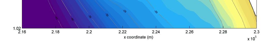
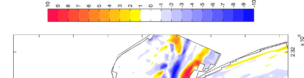
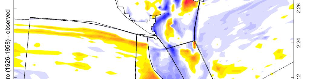
96 Figure 5.1 Observed bathymetry at the end of Period B (1958). Figure 5.2 Observed sedimentation-erosion plot for Period B ( ). 86 of 145

97 Figure 5.3 Modeled bathymetry at the end of Period B from the reference simulation (top) and from the Moerman (2011) simulation (bottom). 87 of 145

98 Figure 5.4 Modeled sedimentation-erosion plots for Period B, reference simulation (top) and Moerman (2011) simulation (bottom). 88 of 145

99 5.1.1 Bathymetric changes Quantitative volumetric changes in the earlier defined compartments for the observed bathymetric change, modeled change and model results in Moerman (2011) are given in Table 5.1. A more extensive description of the morphological change per compartment for both long-term simulations is given below. Compartment Observed Reference simulation Inlet Mm Mm 3 (+20.8%) Mouth -0.4 Mm Mm 3 (-) Peacock Spit Mm Mm 3 (-2.1%) Erosive part Mm Mm 3 (+54.1%) Deposition part Mm Mm 3 (+14.2%) Long Beach Mm Mm 3 (-2.1%) Clatsop Spit Mm Mm 3 (-30.4%) Table 5.1 Computed volumetric changes and relative errors for Period B. Moerman (2011) simulation Mm 3 (+32.6%) Mm 3 (-) Mm 3 (+16.0%) Mm 3 (+57.3%) Mm 3 (+28.1%) Mm 3 (+42.2%) Mm 3 (-165.1%) Inlet and river In the reference simulation, a generally wider and more southern orientated inlet channel developed in the inlet compartment. The MCR entrance channel is also shallower in the model results. Erosion near the North Jetty and the development of a scour hole near Jetty A are less severe in the simulation results, but both are present in the final bathymetry. The maximum depth near Jetty A is less than 25 meters in the reference simulation, whereas the observed maximum depth exceeded 30 meters in the inlet. Widening of the entrance channel at the southern side consequently resulted in erosion of Clatsop Spit. The model does not contain the development of some small channels at Baker Bay. Deposition of material west of the South Jetty is quite well represented by the model. The total modeled volume change of the inlet compartment is Mm 3 for Period B. This is an overestimation of 20.8% compared to the observed volume change of Mm 3. The computed volume change in the river compartment is Mm 3, which is an overestimation of 11.8 Mm 3 compared to the observed change in this compartment. Model results in Moerman (2011) show a similar pattern with erosion at the south side of the entrance channel and accretion in the formerly deeper parts. In these results, the volume change in the inlet compartment was overestimated by 32.6%. The new model results thus give a quantitative improvement. When looking at the volumetric change in the inlet compartment over time of the two model simulations (Figure 5.5), it appears that the difference is small relative to the total change. It seems that no equilibrium situation with respect to the volumetric change of the inlet compartment is yet reached at the end of the model simulations, as the rate of change does not approach zero at the end of the simulation. The rate of morphological change does however decrease during the simulation period. 89 of 145

100 Especially in the first couple of years, a strong initial response is present in both model simulations. Peacock Spit The modeled bathymetry at the Peacock Spit compartment shows some clear differences compared to the observed bathymetry. Large deviations are visible near the North Jetty where a shallow northwestern directed channel seems to have formed as a result of the confined ebb-flow. This development of a northward channel occurred as an initial response in the simulation. During the simulation, this process stopped and reversed causing the shallow channel to fill up again. Remains of the northern orientated channel are however still visible in the model results. A scour hole developed near the North Jetty head, where ebbvelocities are highest. In the observed bathymetry, the scour hole is located more at the south side of the North Jetty head. The remains of the Peacock Spit shoal are located more to the north in the model results. In the observed bathymetry, the southern edge of the shoal is in line with the North Jetty, whereas the model results show a clear remainder of the shoal south of this imaginary line. The observed erosion in the nearshore area just north of the North Jetty is also visible in the model results. Total computed change in the Peacock Spit compartment is Mm 3, an underestimation of just 2.1%. A volume change of Mm 3 is reached after 32 years in the erosive part of the Peacock Spit compartment, while the observed volume change of Mm 3 was less (+54.1%). Deposition of material northwest of the MCR is more concentrated and located more to the north in the reference simulation compared to the observed bathymetry. Deposition further offshore is barely represented by the model. A total volume change of Mm 3 is computed, while the observed volume change was Mm 3 (+14.2%). The location of the Peacock Spit and Long Beach polygons and consequently the volume change within the polygons are not corresponding exactly with the areas of deposition and erosion. However, the total volumetric changes in both polygons combined (Peacock Spit and Long Beach combined) is an accurate measure for the volumetric change in the area north of the MCR. Model results in Moerman (2011) give similar patterns of bathymetric change. The channel-forming west of the North Jetty was however less pronounced in that model simulation. Consequently, the remains of this northern orientated channel are not as clearly visible in the final bathymetry. The model simulation in Moerman (2011) gave a larger deviation of +16.0% with respect to the volumetric change in Peacock Spit compartment. Volumetric change within the erosive part in Moerman (2011) was comparable to the volume change in the reference simulation. In the depositional part, the Moerman (2011) simulation gave an overestimation of 28.1% compared to the observed change. The rate of change (Figure 5.5) decreases throughout both simulations after a large initial response. This might be a result of the channel-forming west of the North Jetty, which occurred as an initial morphological response in the model and pushed large amounts of sediment to the north. As the model simulations continue, this process stopped and reversed. Long Beach The modeled morphological change at the Long Beach sub-cell consists mainly of deposition at the northern edge of Peacock Spit and at nearshore areas. Some shoreline progradation is visible in the model results, but the grid resolution is too low to quantify this coastal advance. Little morphological change is visible in the offshore parts of the Long Beach compartment. The total modeled volume change in this compartment is Mm 3, similar to the observed volume change of Mm 3. The volume change rate (Figure 5.5) is quite constant throughout the model simulation, implying that there is a continuous process of net deposition 90 of 145

101 north of the MCR. Model results in Moerman (2011) show a clear deposition band in the nearshore area. The volume change within the compartment gave a large overestimation of the observed volume change (+42.2%). However, a large part of this deposition seems to be caused by errors with respect to sediment mass continuity because of an erroneous schematization of the transition period between consecutive wave conditions (see: Par ). These errors occur especially in the proximity of the breaker zone, where most material gets in suspension due to wave action. The distinct deposition band in the proximity of the breaker zone is one of the indications that this deposition is indeed induced by sediment mass errors. Clatsop Plains In the Clatsop Plains compartment, only little morphological change is visible in the model results. There is some deposition close to the coastline and local erosion on several offshore spots. This pattern is quite similar to the observed sedimentation-erosion pattern. However, the morphological change is underestimated. The modeled volume change in the reference simulation is only Mm 3 while the observed change is Mm 3, an underestimation of 30.4%. In the model results of Moerman (2011), a clear deposition band is visible in the nearshore areas. This might again be induced by sediment mass errors due to the schematization of the transition period between consecutive wave conditions. Because of this, the volumetric change in the Clatsop Spit compartment gave net deposition instead of erosion. The relative error with respect to the observed change is therefore -165%. 91 of 145

102 Figure 5.5 Volumetric change over time for Period B at the inlet (top left), Peacock Spit (top right), its erosion part (mid left), its deposition part (mid right), Long Beach (bottom left) and Clatsop Plains (bottom right). 92 of 145

103 5.1.2 Sediment transport pattern and littoral drift In addition to the above analysis of volumetric changes, the modeled littoral transport pattern is analyzed as well. Several cross-sections are defined through which the mean longshore transport during the long-term simulations is computed. The locations of these cross-sections are at Long Beach, North Head, Peacock Spit, the North Jetty and the South Jetty. A crosssection between the jetty heads is added to quantify the average sediment feeding from the estuary towards the MCR and coastal system. Figure 5.6 shows the mean annual transports through all cross-sections along the littoral cell and the river, obtained with the reference simulation and with the Moerman (2011) model results. Transports are given in Mm 3 per year. The plots also contain the mean total transport patterns for both simulations. No measured data is available for the annual longshore transports, so it is not possible to compare the transport values with the observed situation. However, from a shoreline modeling study (Ruggiero et al., 2010), it followed that the longshore transport just north of the North Head rocky promontory should be about 1.4 Mm 3 /yr to account for the Long Beach shoreline change from the 1950s and on. Besides, Byrnes et al. (2007) suggested general transport pathways based on sediment budgets of the MCR area for the period. Figure 5.6 Modeled transport patterns and transports through cross-sections (in Mm 3 yr -1 ) for Period B, obtained from the reference simulation (left) and the Moerman (2011) simulation (right). 93 of 145

104 When looking at both mean sediment transport patterns, it can be seen that the model simulations contain a strong northwestward-directed transporting pattern at the river. Transports concentrate near the jetties, where distinct scour holes developed. Sediment enters the central MCR area from the south and from the Columbia River inlet area and is transported mainly to the north. Over there, the sediment contributes to the northwest development of the ebb-tidal delta. Just north of the North Jetty a circular pattern can be observed. Sediment flushed through the river by the strong ebb-flow might end up in this eddy-like pattern. Further northwest on Peacock Spit some differences between the simulations can be observed. The new Period B simulation contains a clear transport pattern in direction of the Long Beach coastal sub-cell, whereas the Moerman (2011) simulation does not show much interaction with the coastal cell at all. In the inlet area (between the jetties), an exporting transport pattern is visible in both simulations. Only on Clatsop Spit, directly adjacent to the South Jetty, an importing pattern can be observed. The modeled littoral transports show an alongshore variation with higher transport rates near the MCR. This can also be observed in Figure 5.7, which shows a graph of the modeled littoral drift (or alongshore directed transports), obtained from the reference simulation and from the Moerman (2011) simulation. The net littoral drift is directed northward throughout the entire system. At the southernmost part of the model domain, transport rates might be influenced by the open boundary through which material is entering the model domain. In reality however, a large rocky promontory that prevents sediment entering the system is present just south of the model boundary. At Clatsop Plains, the modeled littoral drift is approximately 1.3 Mm 3 /yr and northward directed. This value is 50% higher than the sediment inflow from the south of about 0.8 Mm 3 /yr that was hypothesized by Byrnes et al. (2007) for the interval. Transport rates strongly increase near the MCR, where more sediment is available and getting in suspension due to the presence of the ebb-tidal shoal and additional sediment feeding from the Columbia River. Highest longshore transport rates are found west of the North Jetty (4.1 Mm 3 /yr) and on Peacock Spit (3.7 Mm 3 /yr), associated with the large morphological change that occurred at the ebb-tidal shoal during Period B. At the cross-section near North Head the modeled littoral drift is 1.7 Mm 3 /yr, little higher than the estimated value for Period C just north of North Head in Ruggiero et al. (2010). Further up north at the Long Beach cross-section, the modeled transport rate gradually decreases to values around Mm 3 /yr. The computed mean annual sediment feeding from the estuary and inlet area towards the MCR and the littoral system is 1.7 Mm 3 /yr, measured between the entrance jetty heads. Mean annual transport rates obtained from the Moerman (2011) model results are all lower than the newly modeled transports. The highest longshore transport rates are again found west of the North Jetty (2.9 Mm 3 /yr) and on the Peacock spit shoal (2.0 Mm 3 /yr). In the Long Beach coastal cell, lower transport values are found. The mean annual transport passing North Head was only 0.4 Mm 3 /yr in this model, while a value of 1.7 Mm 3 /yr is found with the new model simulation that is schematized with a wave climate that is generated based on the longshore transport pattern. At the coastal sub-cells, the computed mean transports were only Mm 3 /yr. The sediment input from the estuary and inlet towards the littoral system is computed to be 1.5 Mm 3 /yr on average with the Moerman (2011) model results, comparable to the values found in the new model results. 94 of 145

105 Figure 5.7 Modeled littoral drift along the CRLC. 5.2 Model performance The model results obtained in this study represent the observed morphological development of the MCR and adjacent coasts fairly well, both in a qualitative and quantitative manner. The model does represent the approximate locations of morphological features and distinct sedimentation or erosion areas. Deviations are however visible near the North Jetty head where a shallow northerly orientated channel formed and filled up again during the simulation. A general erosion pattern in the inlet and inner delta compartment is visible. The eroded material is mainly deposited at the outer delta and Long Beach compartments. Deposition of material further offshore is hardly present in the model results. Some features that are well represented by the model are the erosive pattern on the Peacock Spit shoal, the development of a scour hole at the head of the South Jetty, deposition at the eastern part of Clatsop Spit and north of the inlet channel and the nearshore deposition and apparent coastal advance in the Long Beach sub-cell. The model also captures the interaction between the ebb-tidal delta area and the adjacent Long Beach coastal sub-cell. A clear area of deposition stretching from the outer delta compartment through to the Long Beach coast is present. Besides, the volume deposited at the Long Beach sub-cell corresponds fairly well with the observed volume change, implying that the amount of material is transported from the MCR area towards the Long Beach subcell is approximately right. However, in the observed erosion-sedimentation plot the accumulation of material in the Long Beach compartment is more spread out over the offshore parts within the polygon. The computed mean transport pattern cannot be compared with measured data. Nevertheless, the littoral drift north of the river entrance is probably represented reasonably well, as the computed transports do account for quite accurate volume changes in the Long Beach and Peacock Spit compartments. Besides, the computed annual transport rate near North Head is of the same order as the hypothesized value in Ruggiero et al. (2010) for the 1950s-1990s interval. The volumetric change in the defined compartments is generally overestimated in the new model results. The overestimation of the volume change ranges between -30% and +50%. 95 of 145

106 The net erosion in the erosive part of the Peacock Spit compartment is overestimated by the highest value of 54%. This is despite the fact that lower limit transport factors and relatively course sediment fractions were used. For this study, the overestimations in volumetric change are considered to be within acceptable range. Contrary to the pattern of overestimating the morphological change, the overall erosion in the Clatsop Plains compartment is underestimated by 30.4%. Some major deficiencies are present in results as well. The deficiencies discussed below are: the formation of a wider and shallower channel between the inlet jetties and therewith erosion at the Clatsop Spit shoal; the formation of a shallow and northern orientated channel through Peacock Spit in the initial phase of the simulation (Over time, this channel is largely filled up again); the more northern orientation of the Peacock Spit shoal in the modeled bathymetry; missing the offshore deposition northwest of the MCR area in the model results. The formation of a wider and shallower channel between the entrance jetties is one of the main differences between the observed and modeled bathymetry. Besides, the channel is also positioned slightly more to the south in the model, which induces erosion at the northern flank of Clatsop Spit. Possible explanations for the relatively wide and shallow channel could be omission of dredging activities in the Period B simulation and the bed level schematization with a relatively course sediment fraction in the inlet channel. Presence of a too course sediment fraction can lead to a more shallow entrance channel, as higher current velocities are necessary to induce erosion at the channel bed. By this means, the course sediment fraction on the entrance channel bed could indirectly have contributed to the erosion of the shoal south of the channel where some finer fractions were present as well. Omission of early dredging activities is another possible reason for the poor channel representation. Dredging activities are performed to maintain the channel bathymetry and depth and may force the entrance channel to adopt a certain path instead of letting it seek its own orientation. However, the wider entrance channel also formed in the Period C simulations with dredging activities (see: Section 6). Therefore, this explanation for the development of a wider channel is considered unlikely. Another explanation could be the presence of Jetty A during the entire simulation, whereas in reality this jetty was not present before Jetty A forced the channel in a more southern configuration. Therefore, its presence in the initial phase of the model simulation might have affected the configuration of the entrance channel. Breaching of the South Jetty that occurred during Period B is not included in the model schematization either. These breaches might also have affected the Clatsop Spit morphology. A second major deficiency in the model is the formation of a northerly-orientated channel through the Peacock Spit shoal in the initial phase of the simulation. This channel forms directly west of the North Jetty and heads in a northwest direction. Its emergence seems to be an indirect result of the widening of the channel between the jetties. As the channel widens and erodes the northern flank of Clatsop Spit, a large amount of sediment is pushed out of the inlet area. The material then partly blocks the entrance channel and causes the entrance channel to adopt a different configuration, which in this case is in a more northwestern direction. When the entrance channel between the jetties has adjusted and the southwestern channel fully opens up again, the northwestern channel starts to fill up and disappear. An explanation for this phenomenon could again be the omission of early dredging activities in this simulation. Dredging activities could prevent a northern directed channel from developing by maintaining the southwestern directed entrance channel. The initial bathymetry seems to have a large impact on the emergence of the channel as it did not appear in such pronounced 96 of 145

107 form in the Period C simulations (see: Section 6). Widening of the entrance channel and the amount of erosion on the northern flank of Clatsop Spit associated with this widening are probably the most dominant factors for this process. Peacock Spit itself has a more northern orientation in the model bathymetry. In the observed 1958 bathymetry, the Peacock Spit shoal is orientated in line with the North Jetty, whereas the shoal dispersed more to the north in the model results. Tide-induced flow through the northerly-orientated channel probably transported material in this direction. The limited representation of offshore deposition northwest of the MCR can mainly be addressed to the schematization of the hydraulic forcing conditions and the schematization of sediment fractions. Buijsman et al. (2003) already hypothesized that the offshore deposition is probably caused by extreme discharge conditions in the Columbia River such as the 1948 peak flow. During extreme discharges, a plume of fine sediments is released by the Columbia River. As extreme discharges are missing in the schematization of the river discharge, the offshore deposition caused by them is missing as well. Offshore deposition is also limited by omission of very fine sediments in the model schematization. In addition to above model deficiencies, several smaller deviations are present in the model results. Some minor sedimentation or erosion spots are not represented well or differ in location compared to the observed situation. Most probable causes for these differences are the schematization of both hydraulic forcing conditions and the sediment fractions. Extreme discharge conditions are not implemented in the model schematization, neither are the highest wave conditions. The highest wave condition used in the model wave climate is a 7.45 m condition coming from the southwest. In reality, offshore wave conditions of over ten meters can occur in the CRLC during severe storms. In general, using only 15 wave conditions means some conditions are averaged out or missing in the final schematization. The same holds for the schematization of the bed, for which only two sediment fractions were used. This rather rough schematization can easily lead to local differences in the morphological behavior. Other causes for local differences might be the seasonal character of hydraulic forcing conditions and therewith the shoreface profiles. 5.3 Model comparison The model results obtained with the new model schematization differ on several points from the results obtained in Moerman (2011). Especially in the compartments of the adjacent coastal sub-cells, some clear differences are visible. At the MCR inlet area itself on the other hand, the resulting bathymetries are quite similar. The main differences are discussed below. When comparing the results quantitatively, it appears that the new model schematization successfully helped reducing the tendency of the model to overestimate the morphological change. The new model results give an equally as good or better representation of the volumetric changes for all compartments. Besides, the model now contains a better interaction between the ebb-tidal shoal of Peacock Spit and the adjacent coastal cell. The littoral drift seems to be better represented compared to the former model results as a clear area of deposition between the shoal and Long Beach is generated, indicating that material from the shoal is indeed feeding the coastal cell. This area of deposition and feeding pattern is hardly present in the Moerman (2011) model results. Besides, the mean longshore transport rate increased with the new model schematization and now corresponds fairly well with the suggested values in Ruggiero et al. (2010) and Byrnes et al. (2003). The new wave 97 of 145

108 climate schematization, which was obtained by focusing on both the MCR and the alongshore transports, is considered to be the main reason for these improvements. Major differences between the model results are visible in the compartments of the Long Beach and Clatsop Plains coastal cells. In the new model results, some nearshore and onshore deposition is visible. Further offshore not very much morphological change occurs, except for the earlier mentioned area of deposition north of the Peacock Spit ebb-tidal shoal. In the model results obtained from Moerman (2011), clear areas of deposition are visible in the proximity of the breaker zone of both the Long Beach and Clatsop Plains coasts. It is however suspected that these deposition bands are a result of errors with respect to continuity of sediment mass (see also: Par ). Low longshore transport rates and positive transport gradients in the Long Beach sub-cell in combination with large amounts of deposition indicate that sediment mass errors are indeed present in the former long-term model simulations. Because of this deficiency, simulation results obtained with the new schematization are considered more trustworthy. This holds especially for the coastal areas, where waves play a major role. Another distinct difference in bathymetry can be observed on Peacock Spit, west of the North Jetty. The remains of the initial northwestern channel forming are still clearly visible in the new model s final bathymetry, whereas these remains are less pronounced in the final bathymetric result of the Moerman (2011) simulation. The schematization of the wave climate is again considered the main cause for this difference. The newly derived wave climate contains more high-energy wave conditions, especially from a southwestern direction. These wave conditions might have increased the channel-forming pattern in the initial phase of the simulation. High-energy wave conditions can, depending on their approach angle, enforce or weaken the tide-induced transport pattern that is mainly responsible for the channel forming on Peacock Spit. Using a relatively calm wave climate, as in Moerman (2011), may therefore help to reduce the incorrect initial morphological response that is present in the model. Apart from the differences mentioned above, the newly obtained and Moerman (2011) model results are comparable. Since the morphological development in the inlet and estuarine areas is mainly driven by the tide and the morphological tide is schematized in an identical way in both models, no major differences were to be expected. Conclusion Despite some deficiencies that are still present in the new model results, some major improvements have been achieved with the new model schematization. Especially the morphological interaction with adjacent coastal cells has been improved. Sediment mass errors have been taken out, which led to a better and more realistic representation of the deposition pattern in the coastal sub-cells, adjacent to the MCR. Improvements have also been obtained quantitatively with respect to the representation of total volumetric change in the defined model compartments and the longshore transport pattern. Downside of the new model schematization is the northward-directed channel which develops in the initial phase of the simulation and is still partly visible in the final bathymetry. Nevertheless, it can be said that the overall model performance has been improved by applying the new schematization. Therefore, the new model setup and hydraulic boundary conditions will be used for the Period C ( ) model simulations and for the analysis of the impact of dredging and disposal activities on the MCR morphological development. 98 of 145

109 5.4 Analysis of alternative model schematizations Several additional model simulations are performed to analyze the influence of alterations in the model schematization and possibly improve the model s performance. The results of these model simulations are discussed in more detail in Appendix G. A brief overview of the additional simulations is given below. Simulation with a seasonally varying wave climate Firstly, a simulation in which seasonal variation is performed by rearranging wave conditions is used to see whether the order of wave conditions or seasonality have a significant influence on the simulation results (Appendix G.1). It appears that the sequence of wave conditions does not have a significant influence on the long-term morphological changes. The seasonally varying wave climate is again used for the Period C simulations with dredging and disposal activities included as seasonality might still be important for the direction in which disposed material disperses. Simulation with a reduced MorFac in the initial phase of the simulation In an attempt to reduce the high initial morphological response of the model, a simulation is also performed with reduced morphological scale factors in the initial phase of the simulation (Appendix G.2). There are no clear differences found between the model results after a morphological period of ten years. Applying reduced morphological scale factors in the initial phase of the model simulation does increase computation times significantly and it does not reduce the initial morphological response or improve the model results in general. Therefore, it is not used for further model simulations in this study. Simulation with an altered initial sediment distribution at the MCR A simulation with a manually altered initial sediment distribution is performed (Appendix G.3). This schematization contains a more realistic distribution of the two sediment fractions, especially in and around the ebb-tidal delta. Application of this alternative bed schematization with finer fractions on the ebb-tidal delta leads to a local increase of volumetric changes and sediment transport rates. The morphological changes are thereby overestimated more than in the reference simulation. It appears that the model results are very sensitive for the initial sediment distribution. A more detailed (possibly three-dimensional) bed schematization might well lead to better morphological results. Simulation with enhanced bed load transport factors A simulation with changed sediment transport factors for bed load transport is performed as well (Appendix G.4). From this simulation, it appears that further calibration of the bed load transport factors can be used to regulate the onshore feeding from the ebb-tidal delta towards the coastal cells and the cross-shore sediment balance in general. 99 of 145

110

111 6 Period C simulations ( ) Influence of dredging and disposal activities The Period C ( ) long-term simulations are used to analyze the influence of historical dredging and disposal activities on the morphological development of the MCR and adjacent coasts. Simulations are performed in which no dredging or dumping activities are included, in which only dredging is implemented and in which dredge and disposal activities are both implemented. By comparing the results of these simulations, the influence of dredging and disposal activities is assessed. The configuration of the Delft3D-model is kept constant to the settings of the simulations, but the duration of the model simulations is elongated to four consecutive standardized wave climates (see also: Par. 3.9). The MorFac values are adjusted slightly to account for the exact 41-year simulation period. In order to be able to implement dredging and dumping activities adequately, the seasonal varying wave climate (Appendix G.1) is used for the Period C simulation with disposal activities included. It has been shown that changing the order of wave conditions does not affect the modeled morphological development of the MCR significantly. Seasonality of the wave climate might still have an influence on the dispersive behavior of dredged material that is placed at the disposal sites. Dredge and disposal activities are only turned on during a limited time span within the simulation. The period during which these activities are active in the model simulation corresponds with late summer in the schematized seasonal varying wave climate. Hereby, it is intended that the dispersion of placed material takes place under similar circumstances (i.e. wave conditions) as it would have in reality. An assessment is made in which different sediment fractions and a combination of sediment fractions are used as dumping material in the model simulation (Par ). The schematization that gives the most realistic model results, a mixture with 50% of the 200 m fraction and 50% of the 500 m fraction, is used to analyze the influence of disposal activities at the MCR. Finally, the model results are discussed in Par Analysis of the model results Resulting bathymetries and sedimentation-erosion plots for all three simulations are shown in Figure 6.1 and Figure 6.2. The observed 1999 bathymetry and sedimentation-erosion plot for Period C are repeated in these figures as well. Difference plots have been made as well (Figure 6.3). From these plots, which give the difference in bed level and difference in mean total transport patterns between the three simulations, the net influence of dredging and disposal can be analyzed. The polygons used for dredging and disposal of dredged material are included in these figures. Several compartments are again defined for which the volumetric change is calculated. All compartments are shown in the sedimentation-erosion plots and are similar to the compartments used for the analysis of the Period B model results. A separate Site B compartment is defined for the model simulation in which disposal activities are included to distinguish deposition at the disposal site and deposition at the outer part of the Peacock Spit shoal. Transport patterns for the three schematizations are shown in Figure 6.6. Table 6.1 gives volume changes for each compartment and each model simulation. The volumetric changes over time for each compartment are given in Figure 6.4. Site B is in this plot included in the Peacock Spit shoal compartment. A more extensive description of the morphological change per compartment for the model simulations is given in Par of 145

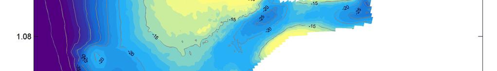
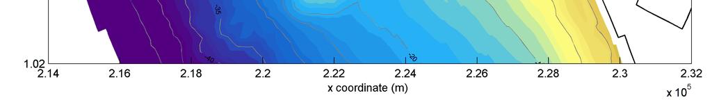
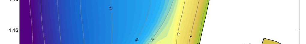
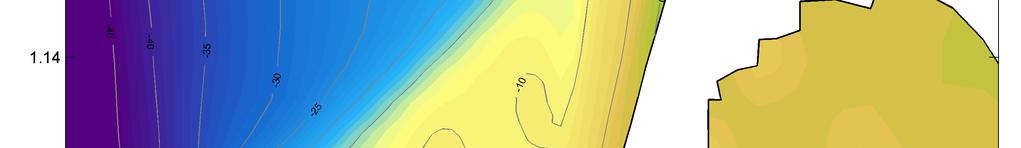
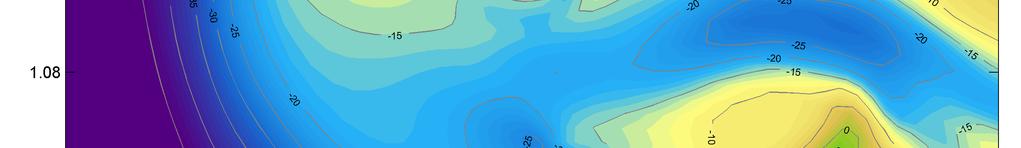
112 102 of 145

113 Figure 6.1 Observed bathymetry (previous page, top) and modeled bathymetry at the end of Period C without dredging activities (previous page, bottom), with only dredging included (top) and with dredging and disposal included (bottom). 103 of 145

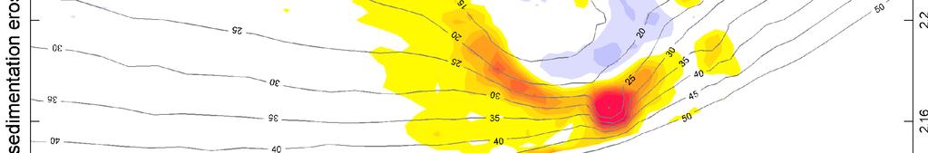
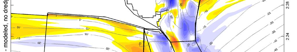
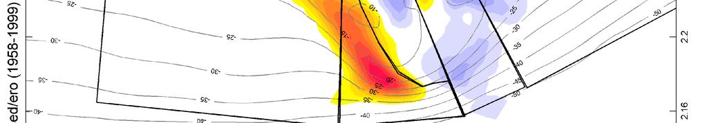
114 104 of 145

115 Figure 6.2 Observed (previous page, top) and modeled sedimentation-erosion plots for simulation without dredging activities (previous page, bottom), with only dredging included (top) and with dredging and disposal included (bottom). 105 of 145

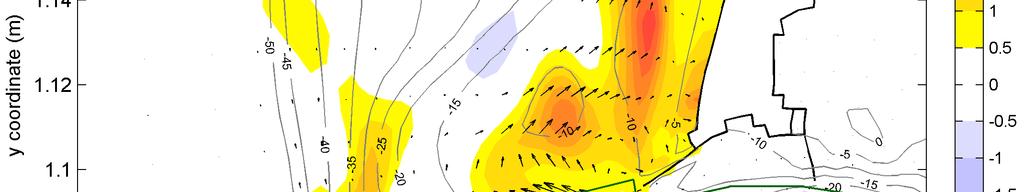
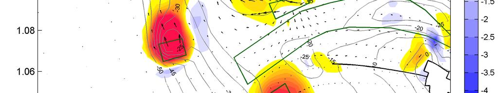
116 106 of 145

117 Figure 6.3 Difference plots showing the bed level difference and mean total transport difference between the simulation with only dredging included and the simulation without dredging activities (previous page, top), between the simulation with dredging and disposal included and the simulation with only dredging (previous page, bottom), and between the simulation with dredging and disposal included and the simulation without dredging activities (above). Compartment Without dredging Only dredging Dredging & disposal Inlet Mm Mm Mm 3 Mouth Mm Mm Mm 3 Peacock Spit Mm Mm Mm 3 - Erosion part Mm Mm Mm 3 - Deposition part Mm Mm Mm 3 - Site B Mm 3 Long Beach Mm Mm Mm 3 Clatsop Plains Mm Mm Mm 3 Table 6.1 Computed volumetric changes for Period C. 107 of 145

118 Figure 6.4 Volumetric changes over time for Period C at the inlet (top left), Peacock Spit (top right), its inner parts (mid left), Long Beach (mid right) and Clatsop Plains (bottom left). 108 of 145

119 6.1.1 Modeled morphological changes An overview of the modeled bathymetric changes and sedimentation-erosion patterns per compartment is given below. A visual analysis is given of the modeled bathymetric results as well as a quantitative analysis of the morphological development by analyzing the computed volumetric changes in the defined polygons (Table 6.1). By comparing the model results with each other, the influence of dredging and disposal activities is analyzed. Inlet and area Just as for the Period B simulations, the channel between the jetties has widened in all model simulations for the period. The entrance channel depth ranges from about 20 meters between the jetties heads to over 25 meters just south of Jetty A. Widening of the channel occurred along with erosion of the northern flank of Clatsop Spit, north of the South Jetty. The scour hole south of the North Jetty head that is present in the observed bathymetry is only visible in the model results of simulations with dredging activities included. In the model simulation without dredging activities, a distinct spot of deposition is present in this area. Model simulations in which dredging activities are included and wherein the southern channel towards the estuary is maintained give less erosion at the northern part of the channel. This phenomenon is clearly visible in the difference plot between the model simulations without dredging activities and with dredging activities included (Figure 6.3). Dredging activities may thus have a great influence on the behavior of the channel configuration at the estuarine side of the MCR. The difference plot between the simulation results with and without dredging activities also shows a clear difference near the North Jetty head, representing the scour hole that is present there if dredging activities are included. Erosion west of the river entrance ranges from about -1 to -5 meters and varies between the model simulations with and without dredging activities. This can also be observed in the difference plot, wherein an additional erosion of -0.5 to -1.5 meters is visible for the situation in which dredging activities are implemented in the model. Near Site A, southwest of the South Jetty, some mounding can be observed when disposal activities are included. However, material placed at this site seems to have dispersed in all directions as the area of deposition (or the polygon in which the material was placed) depleted. Dispersion of material placed at Site A caused erosion west of the South Jetty to decrease slightly. The total volume that is dredged from the entrance channel in the simulation in which only dredging is included is 34.2 Mm 3. When disposal activities are added too, the total dredged volume during the entire simulation increases slightly to 35.3 Mm 3. The total dredged volume at the MCR entrance channel during Period C (about 120 Mm 3 ) is highly underestimated by the model simulations. Underestimation of the dredged volume in the model is a result of the schematization of dredging and disposal in the model simulation (Par. 3.12). Dredging is implemented by prescribing a threshold depth and not by prescribing the exact volumes that have to be dredged. By using this schematization, a realistic navigation channel depth is assured. Downside is that the amount of dredged material can be inaccurate if accumulation of sediment in the navigation channel happens at much faster or slower rates than it does in reality. Missing fine sediments in the bed schematization could be a reason for the low accumulation rate of the MCR channel in the model results. In the estuary domain, courser sediment fractions are applied in the bed schematization to prevent channel and shoal configurations from changing during the long-term model simulations. Due to this method, the sediment inflow from the estuary seems to be underestimated. Using a more realistic and detailed schematization of the bed and sediment fractions could well lead to a better model performance, especially with respect to sediment import into the dredging channel. In Par. 109 of 145

120 6.2.2, the influence of applying a finer sediment fraction in the estuarine domain for the total dredged volume during the model simulation is analyzed. When looking at the computed volumetric changes in the inlet area during Period B, it appears that dredging activities only led to a net additional erosion of about 4 Mm 3 to 6 Mm 3 (see: Table 6.1). The erosion volume in the simulation without dredging activities is about -55 Mm 3, whereas the computed erosion volume in the model simulations with dredging activities is -59 Mm 3 to -61 Mm 3. This implies an increase of the inlet erosion of approximately 10% due to dredging activities. In the river compartment, west of the inlet area, the computed volume change for the simulation without dredging activities is Mm 3. Adding dredging activities leads to an increase of the net erosion to Mm 3. The simulation with dredging and disposal activities gives a net volume change of Mm 3. These values are dependent on the amount of material that is dredged from the MCR channel and do therefore not represent the net influence of dredging activities accurately. Peacock Spit The modeled erosion-sedimentation patterns in the Peacock Spit compartment for Period C show large similarities with the Period B model results. Again, the southern part of the Peacock Spit shoal is eroding and the material is mainly deposited northwest of the shoal. The modeled erosion at Benson Beach and the nearshore areas west of Benson Beach ranges from 1 to 6 meters. Dredging activities have an increasing effect on the erosive behavior of this area (Figure 6.3). When disposal of dredged material is included as well the erosive behavior decreases, as 43.5 Mm 3 of sand was actually placed on the ebb-tidal shoal at Site E (or SWS). Disposal of dredged material at Site B does not have a decreasing effect on the erosion pattern at the western side of Peacock Spit. Material placed at this disposal site did only disperse little to the north, but mainly mounded at the disposal site itself. Deposition in the outer delta compartment is more or less similar for all model simulations. A clear area of deposition is visible northwest of the MCR. It stretches from about 8 km west of the North Jetty in northeast direction to the Long Beach coastal sub-cell. Adding dredging activities in the model schematization induces a slight increase in outer delta deposition, probably because more fine sediments become available for erosion through dredging activities. Finer sediments in layers under the upper transport layer, that normally would not be available for erosion, get exposed as the upper layer is removed by dredging activities. From a visual analysis of the sedimentation-erosion plots (Figure 6.2), it appears that the computed volumetric changes give an overestimation of both the erosion as well as the deposition at Peacock Spit. For the situation without dredging activities, net volume change at the erosive part of Peacock Spit is Mm 3 and the deposition at the outer edge of the shoal is Mm 3. Adding dredging activities increases the net erosion of the inner delta to Mm 3, whereas the total outer delta deposition remains more or less constant at a value of Mm 3. If disposal activities are added as well, the erosive behavior of the inner delta decreases again to Mm 3. Outer delta deposition increases to Mm 3 when adding disposal activities to the Period C simulation. This value does however include the depositional area at Site B. Total deposition at Site B in the model simulation with disposal activities included is 40.2 Mm 3, which is comparable to the observed accumulation of 45.8 Mm 3. When analyzing the net volumetric change of the Peacock Spit compartment, it appears that dredging and disposal activities together did not have a significant net effect on the sand volume of the ebb-tidal shoal. The net volume change of the Peacock Spit compartment was Mm 3 in the simulation without dredging- and disposal activities and Mm 3 in the 110 of 145

121 simulation in which these activities were both included (not including the deposition at offshore disposal Site B). This implies an increase of 11.5 Mm 3 with respect to the sand volume of the Peacock Spit shoal. The volumetric change over time for Peacock Spit and the inner part of the shoal in particular shows clear steps as a result of sand disposal at Site E (Figure 6.4). Net volume gains can also be observed in the difference plot between the model simulation with dredge- and disposal activities included and the model result without dredging activities, in which a slight bed level increase is visible on the inner part of the shoal (Figure 6.3). Some additional deposition is present on the northwestern edge of the ebb-tidal shoal as well and erosion on the western edge of the shoal seems to have increased a little. However, when looking at dredging and disposal activities separately, some clear deviations are observed on the Peacock Spit shoal. The difference plots show distinct additional erosion on the ebb-tidal shoal when only dredging is added and additional deposition when disposal of dredged material is added to the shoal on disposal sites B and E. The computed additional loss of the Peacock Spit sand volume during Period C due to dredging is about 18 Mm 3 as the net deposition in the compartment decreased from 61.7 Mm 3 to 43.6 Mm 3. Again, the influence of dredging is highly underestimated in the model results, as the amount of material that is removed from the model through dredging is only 30% of the volume that was dredged in reality. Long Beach sub-cell All three the model simulations give a similar pattern of deposition in the Long Beach sub-cell. The area of deposition stretches from the northern edge of the Peacock Spit shoal to nearshore and onshore areas further up north. Deposition at Long Beach can be observed up until the 15 m depth contour. Only little shoreline advance occurred in the model simulations, especially when compared to the advance of a few hundred meters in the observed bathymetry. Given the fact that the deposition in the outer delta compartment is overestimated in the model results, it seems that the onshore transport from the outer delta and coastal shelf towards the Long Beach coastal cell during Period C is not entirely repreented in the model simulations. Adding dredging activities or disposal of dredged material does not affect the final bathymetric result or the deposition pattern in the Long Beach sub-cell. No distinct bed level differences are present north of the Peacock Spit shoal in the difference plots between the three model simulations (Figure 6.3). The modeled volume change in the Long Beach compartment for the simulation without dredging activities is Mm 3. If dredging activities are included in the simulation, the total deposition remains approximately similar with a net volume change of Mm 3. Disposal of dredged material leads on the other hand to an increase in the Long Beach compartment deposition. Total deposition in the Long Beach compartment is 63.2 Mm 3 for the model simulation with both dredging activities and disposal of dredged material included. This is an increase of about 16 Mm 3 with respect to the other two simulations. The extra amount of deposition due to disposal of dredged material mainly concerned the southern part of the Long Beach sub-cell, near the boundary with the Peacock Spit compartment. The additional deposition could therefore also be attributed to the sand volume of the Peacock Spit shoal and onshore areas directly connected to this shoal. Clatsop Plains sub-cell Modeled bathymetric results show little morphological change during Period C. The shoreline position remains almost similar to the initial position. Only in the northern part of the coastline, some shoreline advance can be observed in the model results. This advance seems to be a direct result of sediment blocking by the South Jetty. Further offshore, no significant bathymetric changes have taken place. An exception is the northern part of the Clatsop 111 of 145

122 Plains compartment, south and southwest of the South Jetty. In this area, an erosive pattern can be seen in all model simulations, as well as in the observed sedimentation-erosion plot (Figure 6.2). The northern part of the Clatsop Plains compartment contains Site A for the disposal of dredged material Mm 3 of sand was placed at this disposal site during Period C. Adding disposal activities in the simulation does therefore lead to a decrease in the erosive behavior in the northern part of the compartment. When analyzing the computed volume changes in the Clatsop Plains compartment, it can be seen that a general erosion pattern is present in all model simulations. Net erosion is calculated to be Mm 3 for the simulation without dredging activities and Mm 3 for the simulation with only dredging included. The volumetric change in the simulation in which disposal of dredged material is added as well is Mm 3, a difference of 12 Mm 3 to 15 Mm 3 compared to the other simulations. This difference can be attributed completely to the dredged material that was placed at Site A. In the observed sedimentation-erosion plot, a deposition area is present at Site A as well. After the disposal activities in the 1980s, the modeled bed level lowers again. The modeled dispersion rates at Site A are in the order of about 1-2 meters per ten years. The dispersion behavior of the mound is assessed in Appendix H, based on the output of the model simulations. The volume change over time in the Clatsop Plains compartment shows a distinct step for the simulation in which disposal activities are implemented (Figure 6.4). This step indicates the impact disposal at Site A on the volume change of the entire compartment. Site F is not included in the model schematization, so the observed accumulation at that site is not present in the model results Modeled sediment transports Plots of the modeled sediment transport patterns for all three simulations are given in Figure 6.6. These plots also contain the mean annual transports through several cross-sections along the littoral cell. Cross-sections are drawn at the South Jetty, North Jetty, the Peacock Spit shoal, North Head and the Long Beach coastal sub-cell to quantify the transport rates at these locations. An additional cross-section is drawn between the entrance jetty heads as well. A graph of the longshore transports throughout the littoral cell for each simulation, including the Period B reference simulation, is given in Figure 6.5. There is no data available for transport rates at the area of interest. However, Byrnes et al. (2007) suggested transport rates based on a sediment budget analysis for the period, which corresponds fairly with Period C in this study. To balance the volumetric changes at the MCR and adjacent coastal cells a sediment input of approximately 0.8 Mm 3 /yr was suggested from the south at Clatsop Plains. Sediment losses up north halfway at the Long Beach peninsula were estimated to be about 1.1 Mm 3 /yr and the average sediment input from the estuary into the inlet area around 3.0 Mm 3 /yr. Ruggiero et al. (2010) also provided estimates for longshore transport rates at the Long Beach sub-cell based on the one-line shoreline change model UNIBEST-CL. At the North Head rocky promontory, a sediment input of 2.3 Mm 3 /yr in northward direction was used as a sediment inflow in this study to account for the shoreline changes during the interval. Just north of this headland, the sediment transport rate decreased to approximately 1.4 Mm 3 /yr to simulate the shoreline advance in this section. A net northward sediment transport rate of 0.4 Mm 3 /yr was computed at the northern boundary of the Long Beach coastal sub-cell. Transport pattern The modeled sediment transport patterns for the Period C simulations is largely similar to the pattern that was obtained from the Period B simulation (Par ). At the MCR, a general exporting pattern is present in the model results. Highest sediment transport rates are found 112 of 145

123 just west of the North Jetty. In the inlet area, a circular pattern arises with net import over the Clatsop Plains shoal and export through the navigation channel. Export through the entrance channel does however decrease when dredging is included. Sediment input from the estuarine domain into the inlet area and sea domain is limited in all three simulations. Absence of a significant sediment inflow from the estuary could be a dominant factor for the relatively small amount of sediment that is dredged from the entrance channel in the model simulations. On the ocean side of the river, the transport pattern switches to a more northern direction as waves get more dominant. At the Long Beach and Clatsop Plains coastal cells, the net littoral drift is directed northward throughout the entire model domain (Figure 6.5). The transport pattern converges in the northern part of Clatsop Plains near the tip of the South Jetty and continues in a north- to northwestward direction across the river entrance. Highest transport rates are then found at the Peacock Spit shoal, where the largest morphological changes occurred. An eddy-shaped circular transport pattern resulting from the strong ebb-flow is present just north of the North Jetty. Further up north at the Long Beach peninsula, transport rates decrease again as sediment is deposited at the northern edge of the ebb-tidal shoal and along the coastal cell itself. Transport rates When looking at the modeled sediment transport patterns quantitatively, it appears that transport rates near the MCR are lower during Period C compared to the values found for Period B based on the simulation without dredging and disposal activities. Conversely, alongshore transports at the Long Beach coastal cell are higher for the Period C simulations. This corresponds with the observation that large-scale morphological changes at the river were more intense in the period directly after jetty construction than they are now. Observed coastal advance in the Long Beach sub-cell was on the other hand higher during Period C than during Period B. For all three the model simulations alongshore transport rates are northward-directed throughout the model domain. They vary from 0.5 Mm 3 /yr in the northern part of the model domain to a maximum of approximately 3-4 Mm 3 /yr at the Peacock Spit shoal. No significant differences in longshore transports can be observed between the three simulations, except for the pattern in the river entrance and on the ebb-tidal shoal. The net northward sediment transport of about Mm 3 /yr at the southern part of the model domain is higher than the 0.8 Mm 3 /yr littoral drift suggested by Byrnes et al. (2007). West of the South Jetty, about 1.5 Mm 3 /yr enters the MCR from the Clatsop Plains sub-cell in all model simulations. Net sediment transport from the inlet area towards the ocean varies between the simulations with and without dredging activities. In the model simulation without dredging activities, a net sediment flux of 1.3 Mm 3 /yr passes through the entrance jetties. When dredging is added, this value decreases to 0.9 Mm 3 /yr. Adding disposal activities as well leads to a further decrease of the net sediment export to 0.8 Mm 3 /yr. A decrease in net sediment export due to disposal activities can be explained by an increase of the gross import when material is dumped at Site E, close to the North Jetty head. The difference plot between model simulations with and without disposal of dredged material does indeed show a slight decrease in net sediment export near the North Jetty, as material placed at Site E is transported into the navigation channel. At the estuarine side of the inlet, the modeled net sediment transports are low. Byrnes et al. (2007) suggested an annual sediment transport of about 3.0 Mm 3 /yr entering the inlet area from the estuary to account for the volumetric changes in and around the MCR. Given the fact that dredging amounts are highly underestimated in the model and the sediment transport from the estuarine domain into the sea domain is much lower than this hypothesized value, it might well be that lack of accumulation of sediment in the dredging 113 of 145

124 channel in the model simulations is induced by an underestimation of sediment supply from the estuary. The amount of material passing the North Jetty in a northward direction varies slightly between the model simulations. If dredging activities are not included, a net sediment flux of 3.6 Mm 3 /yr is obtained. Including dredging activities leads to a decrease of this flux to Mm 3 /yr. Dredging does thus induce a decrease in the net sediment flux entering the Peacock Spit ebb-tidal shoal from the south. On the shoal itself the net sediment transports are affected by both dredging and dumping. Longshore transport rates on the Peacock Spit shoal vary between 2.0 Mm 3 /yr near North Head and 4.0 Mm 3 /yr on the central part of the shoal for the simulation without dredging activities. Adding dredging activities lowers the net longshore transports up to 20% to values of Mm 3 /yr. Disposal of dredged material at Site E completely reverses the modeled effect of dredging activities. Longshore transport rates at the Peacock Spit shoal increase again to values similar to the simulation without dredging activities when disposal of dredged material is added as well. Locally, longshore transport rates are even higher than they were without dredging activities. The enhancing effect of disposal activities is significantly larger than the decreasing effect of dredging on the littoral drift in the model results. This is due to the underestimation of the amount of dredged material in the model simulations. On the Peacock Spit shoal and north of Peacock Spit, the modeled transport rates for the three Period C simulations converge again and north of the North Head rocky promontory no significant differences are present anymore. Modeled transports passing this point are approximately Mm 3 /yr, similar to the values used in the shoreline change study by Ruggiero et al. (2010). Farther up north, the littoral drift slowly decreases as sand is deposited along the coastal cell inducing the observed coastline advance. Longshore sediment transport rates of 1.9 Mm 3 /yr to 1.1 Mm 3 /yr at the southern and mid-stretch of the Long Beach peninsula correspond fairly well with the sediment transport rates computed by Ruggiero et al. (2010) and suggested by Byrnes et al. (2007). Figure 6.5 Modeled littoral drift at the MCR and adjacent coastal sub-cells for the simulation without dredging (black), with only dredging included (blue), with dredging and disposal activities included (red) and for Period B (dashed). 114 of 145

125 115 of 145

126 Figure 6.6 Modeled sediment transport patterns for the simulations without dredging activities (previous page, top), with only dredging included (previous page, bottom) and with dredging and disposal included (above). 116 of 145

127 6.2 Additional simulations Additional simulations are performed for Period C to assess the sensitivity for parts of the model input and to optimize the model performance. This includes simulations in which different sediment fractions are used for the disposal of dredged material. From this assessment, the most appropriate schematization is picked for the analysis of the influence of dredging activities. A simulation in which the bed schematization in the estuarine sub-domain is altered is also included as it is suspected that lack of sediment input from the estuary into the inlet area is a main reason for the relatively low amount of material that is dredged in the model simulations Sediment fraction used for disposal activities Disposal of dredged material is schematized separately from dredging activities in the model schematization. Dumping activities are implemented as nourishments for which a certain sediment fraction or a combination of sediment fractions must be prescribed. In reality, average grain sizes of dredged material at the Columbia River Mouth and thereby also of the material dumped at the placement sites vary roughly between 0.22 and 0.28 mm, with relatively courser sediment dredged at the center of the navigation channel and finer material dredged at the flanks of the channel. In the model simulations, the dredged material consists of a combination of the 200- m and 500- m sediment fractions. Three long-term model simulations are performed to investigate which sediment fraction gives the best representation of the dispersive behavior of dumped material in the model. Besides, the model s sensitivity for the grain size used for disposal of dredged material is assessed by this calibration. In these simulations a sediment fraction of 200 m, a sediment fraction of 500 m and a combination of the two with a ratio of are tested. Figure 6.7 shows the resulting bathymetries around disposal sites A (southwest of the South Jetty) and B (west of the Peacock Spit shoal) for all three simulations and the observed situation. Especially in the resulting bathymetries of the simulations in which the courser sediment fraction and the mixed sediment fraction are used for the placement of material, distinct deposition areas can be identified for Sites A and B. Based on a visual comparison between the three modeled bathymetries it is clear that using solely the relatively fine 200- m fraction leads to a strong overestimation of the dispersive behavior of the placed material, whereas using a courser fraction gives more realistic results. This becomes even clearer when a quantitative analysis of the volume changes within the Site B polygon is made. The simulation in which the finer material is used for dumping gives a net volume change of Mm 3 at the Site B compartment. When the courser 500- m sediment fraction or a combination of both sediment fractions is used to schematize placement of dredged material, volume changes in this polygon are 48 Mm 3 and 40 Mm 3 respectively. These values for volumetric changes at the disposal site are both within close range of the observed volume change of 45 Mm 3 at Site B. At Site A, the modeled bed levels of the mound seem to be affected by the overestimated scour west of the South Jetty head. The modeled bed levels at the disposal site are therefore lower in all three simulations. An adequate representation of the volume change at the disposal site itself implies that the model is able to quantitatively reproduce the dispersive behavior of the dumped material. As the combination of both fractions represents the behavior of dumped material fairly well and it matches the dredged material grain sizes more closely than the course fraction only, this schematization is used for the analysis of the long-term morphological development of the MCR and the influence of dredging and disposal activities during Period C. 117 of 145

128 The dispersive behavior of disposal sites is sensitive to the grain size of the material that is dumped. Further calibration of the ratio between the two sediment fractions used or implementation of a separate fraction for dumping could therefore well lead to a very accurate representation of the dispersive character of the disposal sites. For the purpose of this study however, an accuracy of about 10% with respect to the quantitative dispersion of material is found to be sufficient. Figure 6.7 Observed bathymetry (top left) and modelled bathymetries with a 200 m (top right), 500 m (bottom left) and mixed (lower right) sediment fraction used for the disposal of dredged material Finer sediment fraction in bed schematization in estuary sub-domain The amount of material that is dredged from the entrance channel in the simulations with dredging activities included is significantly less than the amount that was actually dredged from the entrance channel during the period by the USACE. Apparently, there is a lack of sediment accumulation in the inlet area in the model simulations. This could be 118 of 145

129 caused by insufficient sediment input from the estuary, as the sediment fractions used for the bed schematization in the estuarine sub-domain are relatively course compared to the material that is present there in reality. Courser sediment fractions were initially used to stabilize channel and shoal positions in the estuary for the long-term simulations. However, application of too course sediment fractions in the estuary could limit sediment transport towards the sea-domain and the MCR channel as sediment transports are dependent on grain size. Therefore, a simulation is performed in which the bed of the entire estuarine subdomain is schematized using a single sediment fraction of 200 m. This is a rough schematization of the average grain size that is present in the Columbia River estuary, wherein median grain sizes vary from about 125 m to 250 m in large parts of the estuary (see: Appendix E). The transport pattern and the amount of dredged material is then compared to the original simulation in which only dredging activities are included. Mean transport patterns at the estuarine side of the MCR obtained with this new schematization and with the original schematization are shown in Figure 6.8. A graph of the cumulative amount of dredged material for both simulations is given in Figure 6.9. Applying a single 200- m sediment fraction in the estuary domain is inconsistent with the bed schematization of the sea domain. The depth of the channels in the estuary is not maintained when a finer sediment fraction is used. It does however provide for a representation of a net sediment supply from the estuary to the MCR. The estuarine sediment input is seen as a boundary condition for the considered study area at the MCR. From the plotted transport patterns, it follows that applying lower and more realistic grain sizes in the estuary domain does indeed affect the mean total transport pattern for long-term simulations. Only little sediment input from the estuary is present when the original distribution of two sediment fractions is applied. Using a single 200- m fraction in the estuary does enhance the sediment transport in the estuary, especially in the channels. In the model simulations, the net sediment input from the estuary into the inlet area increased from 0.3 Mm 3 /yr for the simulation with the original sediment distribution to 1.6 Mm 3 /yr for the simulation in which the single 200- m sediment fraction was applied in the estuary. A distinct exporting pattern is visible in the southern navigation channel. In the northern part of the estuarine side of the inlet, a more complex transport pattern arises. The northern deeper part of the channel is exporting, whereas the shallower mid-section is importing sediment. The majority of the material that is transported from the estuary towards the inlet area will eventually end up in the entrance channel where it is removed by dredging. This results in an additional amount of dredged material, as can be seen in Figure 6.9. The total amount of dredged material with the original sediment distribution during Period C was about 35 Mm 3. With the new bed schematization in the estuary domain, over 84 Mm 3 is dredged from the entrance channel during the entire simulation. Because it takes time before a significant amount of material is transported from the estuary to the MCR channel, only little difference is visible during the first couple of years. In reality, approximately 120 Mm 3 of sand was dredged from the MCR entrance channel during Period C. Hence, the total amount of dredged material is still underestimated by about 20% with the new schematization. 119 of 145

130 Figure 6.8 Modeled mean total transport patterns from simulations with the original spatial distribution of sediments and with a single 200- m sediment fraction in the estuary domain. Figure 6.9 Cumulative dredged material during Period C Implications for the influence of dredging activities on the MCR morphology Applying a finer and more realistic grain size in the estuarine domain does increase sediment export, accumulation in the inlet area and therefore the amount of material that is dredged from the entrance channel in the model simulation. Using a finer sediment fraction in the estuary has little effect on the transport patterns seaward of the inlet area as the additional sediment input of the estuary is mostly dredged from the entrance channel in the model simulation. This does not hold for the model simulation without dredging activities. To properly 120 of 145

131 analyze the influence of dredging activities on the MCR morphology, the 200- m singlefraction distribution for the estuary is also applied to model simulations without dredging activities and with disposal of dredged material included. The results of these simulations and the quantitative analysis of the influence of dredging and disposal activities on the morphological development of the MCR are given below. The modeled bathymetries for the simulations with the altered sediment distribution in the estuary domain are given in Figure Figure 6.11 gives sedimentation-erosion plots. Difference plots giving the bed level differences and mean total transport differences between simulations with and without dredging activities are given in Figure Table 6.2 gives the volumetric changes for all simulations in the polygons that were used for the quantitative analysis of the former simulations as well. Compartment Without dredging Only dredging Dredging & disposal Inlet Mm Mm Mm 3 Mouth Mm Mm Mm 3 Peacock Spit Mm Mm Mm 3 - Site B Mm 3 Long Beach Mm Mm Mm 3 Clatsop Plains Mm Mm Mm 3 Amount dredged Mm Mm 3 Table 6.2 Computed volumetric changes during Period C from simulations with a single 200 m sediment fraction in the estuary. Influence of additional sediment supply from the estuary Model results obtained with the altered bed schematization in the estuary are on some points different from the earlier presented results, but the large-scale sedimentation-erosion patterns remain similar. When looking at the volume changes quantitatively, it appears that differences are present for the simulation without dredging activities. Sediment input from the estuary clearly influenced the morphological development of the MCR. If dredging is included, the majority of the additional sediment input from the estuary is removed at the entrance channel. In the simulation without dredging activities, sediment input from the estuary induces a growth of the Clatsop Spit shoal in northeastern direction. The entrance channel thereby shifts to the north. Adding dredging activities limits this growth of Clatsop Spit, as the dredged entrance channel just north of the shoal acts as a sink for sediment. This effect of dredging is clearly visible in the difference plot between the two simulations (Figure 6.12). The plot shows a net erosive effect of dredging on the southern part of the entrance channel and a net accumulative effect on the northern part of the entrance channel. Net accretion in this case means that erosion of the northern part of the channel that occurs in the simulation without dredging activities is much lower in the simulation with dredging included. 121 of 145

132 A second major difference between the model results with the single-fraction bed schematization in the estuary and the earlier presented results is the amount of sedimentation and erosion at the MCR in general. Because of the additional sediment input from the estuary, erosion volumes decrease and accretion volumes increase at the MCR. Again, this holds especially for the model simulation without dredging activities. For this simulation, sediment volumes in the inlet compartment, river compartment and Peacock Spit compartment increase by 10 Mm 3, 15 Mm 3 and 31 Mm 3 respectively. Smaller volume increases of 7 Mm 3 and 2 Mm 3 are found for the Long Beach and Clatsop Plains compartments. All these increases can be attributed to additional sediment supply from the estuary. If dredging is included, the majority of the additional sediment input from the estuary is removed at the entrance channel by dredging. Consequently, the volumetric differences with the earlier presented quantitative model results (Par ) are smaller. This also implies that the net effect of dredging activities on the MCR morphological development is larger than suggested by the earlier presented model results. Influence of dredging activities The net volumetric changes in the inlet and river compartment are Mm 3 and Mm 3 for the simulation without dredging activities. The simulation with dredging activities included gives volume changes of Mm 3 and Mm 3 for these 2 compartments. Dredging thus leads to an increase of the erosion in the central part of the MCR of about 42 Mm 3. On Peacock Spit, the net volume change of the compartment decreases from Mm 3 for the simulation without dredging activities to Mm 3 for the simulation in which only dredging was included, a volume decrease of 33 Mm 3 due to dredging. If a similar analysis is performed on the volume changes in the Long Beach compartment, the difference found between the two simulations is negligible. Net erosion in the Clatsop Plains compartment increases by about 5 Mm 3 when dredging is included. In total, dredging induces a net volume loss of 80 Mm 3 within all compartments together. Out of this 80 Mm 3, 33 Mm 3 or about 40% represents a volume loss on the Peacock Spit shoal. The rest represents volume losses just seaward of the river, in the inlet area itself and on Clatsop Spit. The total volume difference of 80 Mm 3 between the simulations without dredging activities and with only dredging included does not account for the total 84 Mm 3 that is dredged in the model simulation. The remaining 4 Mm 3 represents a volume loss outside the analyzed compartments, probably in the estuary domain. Influence of disposal of dredged material Including disposal activities in the simulation with the 200- m single-fraction distribution for the estuary gives similar results as the model simulations discussed in Par The difference plot between the model simulation with dredging and disposal activities and the model simulation with only dredging implemented gives a clear indication of the net effect of disposal activities on the MCR bathymetry (Figure 6.12). Disposal at Site E on Peacock Spit counteracts the volume loss induced by dredging activities. The net volume change in this compartment is +91 Mm 3 when dredging and disposal are both included, approximately the same as for the simulation without dredging activities. Disposal of 43.5 Mm 3 of sand on Site E led to a net volume gain of 31.3 Mm 3 of the entire Peacock Spit shoal based on the model results. This implies an efficiency of about 70% for shoaling up Peacock Spit. In addition to the volume gain on Peacock Spit, disposal activities do also induce additional deposition at disposal Site B (42.5 Mm 3 ) and the other compartments. At Clatsop Plains, a net gain of 21.5 Mm 3 is reached compared to the simulation with only dredging included. In the Long Beach compartment net deposition increases with 7 Mm 3. Erosion at the inlet and river compartments decreases by 21 Mm 3. In general, deposition does reverse the negative impact of dredging on the Peacock Spit shoal and in the inlet area. However, the southern and 122 of 145

133 middle part of the Peacock Spit shoal is still eroding when disposal activities are added. Disposal activities induce net volume gains compared to the situation without dredging activities at the Clatsop Plains and Long Beach compartments, mainly because placement sites are located in or near these compartments. In the river compartment just west of the entrance jetties, there is still net erosion when disposal activities are included in the model simulation in addition to only dredging. For the simulation with dredging and disposal activities included, it also holds that the total amount of dredged material is less than the amount dredged in reality. The amount of dredged material from the entrance channel is 97 Mm 3 for the simulation with both dredging and disposal activities included. Compared to the simulation with only dredging implemented, this is an increase of 13 Mm 3. This does not automatically imply that only 13 Mm 3 of the material placed at the disposal sites ends up in the navigation channel. It could also be that material would have been transported from the disposal areas to the entrance channel anyway, even if disposal activities were not included. The material dumped at the disposal sites is then just replacing the material underneath (or around) that would have been transported into the dredged channel otherwise. Therefore, the amounts and volume differences presented in this section do only comprise the net difference between the situation with and without dredging and dumping. In reality, about 120 Mm 3 was dredged, so there is still a lack of accumulation in the entrance channel of 23 Mm 3 or 20%. This is a significant improvement compared to the model results discussed in Par , in which 70% of the accumulation was missing in the dredged MCR channel. Sediment transport pattern Conclusions with respect to the alongshore transport pattern based on the simulations with the 200 m single-fraction distribution for the estuary (Figure 6.13) remain similar to those drawn based on the earlier discussed model results. Dredging activities decreased the net transport from the inlet area towards the Peacock Spit shoal. Disposal activities at Site E reversed this decrease efficiently. The net transports on the Peacock Spit shoal are even higher for the simulation with dredging and disposal included as for the simulation without dredging activities. North of Peacock Spit, the longshore transport rates converge again. Away from the MCR, both in a northern and southern direction, differences between the modeled transport rates are small. Dredging and disposal activities seem to have had limited effect on the transports and sedimentation-erosion patterns south of the South Jetty and north of North Head and Peacock Spit. Sediment supply from the inlet to the seaside of the MCR decreased from 2.1 Mm 3 /yr for the simulation without dredging activities to Mm 3 /yr for the simulations with dredging activities. The modeled longshore transports vary over time throughout the simulations. Figure 6.14 gives the computed transport rates for each decade of the simulation with dredging and disposal activities included. In general, the littoral drift at the coastal reaches decreased over time. The peak in the longshore transport pattern at the MCR did decrease as well. Transport rates did only increase at the northern part of the Peacock Spit shoal. This corresponds with the dispersion of the shoal to a more northern orientation that occurred in the model simulations. Decreasing transport rates at the MCR imply that the relative influence of dredging and disposal activities for the littoral drift at the MCR got larger over time. To illustrate this, Figure 6.14 includes the computed longshore transport rate for the latter interval of the simulation with only dredging activities. The relative impact of disposal activities for this 10-year period is indeed larger than the relative impact over the entire simulation period. 123 of 145

134 124 of 145

135 Figure 6.10 Modeled bathymetry from simulation without dredging activities (previous page, top), with only dredging included (previous page, bottom) and with dredging and disposal activities included (above). 125 of 145

136 Figure 6.11 Sedimentation-erosion plots for simulation without dredging activities (previous page, bottom), with only dredging included (this page, top) and with dredging and disposal activities included (this page, bottom). 126 of 145

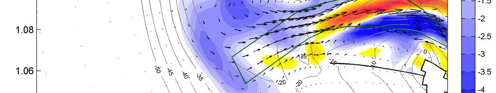
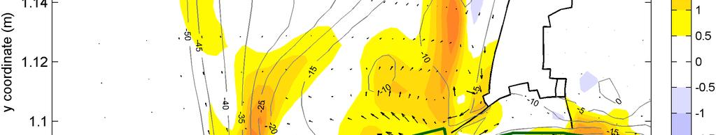
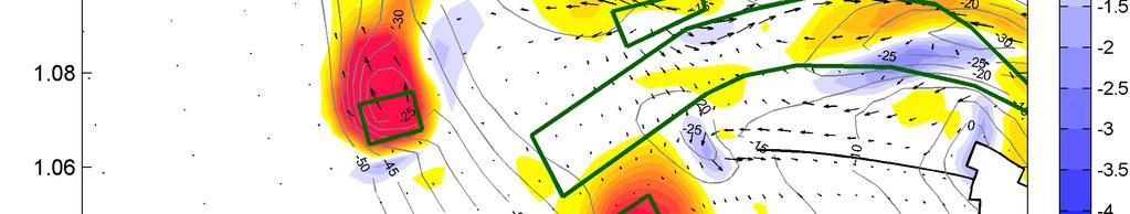
137 127 of 145

138 Figure 6.12 Difference plots showing the bed level difference and mean total transport difference between the simulation with only dredging included and the simulation without dredging (previous page, top), between the simulation with dredging and disposal included and the simulation with only dredging included (previous page, bottom) and between the simulation with dredging and disposal included and the simulation without dredging activities (above). 128 of 145

139 Figure 6.13 Modeled littoral drift at the MCR and adjacent coasts for the simulations without dredging (black), with only dredging included (blue) and with dredging and disposal activities included (red). Figure 6.14 Development of the modeled littoral drift at the MCR and adjacent coasts throughout the model simulation. 129 of 145

140 6.3 Discussion Model performance The or Period C model simulations do represent the large-scale morphological changes (Figure 6.15). The modeled pattern of sedimentation and erosion is similar to the observations. Compared to the Moerman (2010) simulations for Period C, significant improvements have been achieved. Some general morphological features were not represented correctly in this prior long-term modeling study. The major improvement compared to the former long-term process-based modeling study is probably caused by the new schematization of the wave and discharge climate. This newly derived wave climate, containing more high-energy wave conditions, is believed to give a better representation of the alongshore transports and sediment supply from the MCR to adjacent coastal cells. Bathymetric coverage of the 1999 surveys is limited. Making an accurate quantitative analysis of the model s performance is therefore difficult. The quantitative performance of the model was already assessed based on the simulations in Section 5. From that analysis it appeared that the model gives a good quantitative representation of the large-scale morphological development of the MCR. Based on the bathymetric coverage and the quantitative changes that are available for Period C from Buijsman et al. (2003) and Kaminsky et al. (2010), some additional conclusions can be drawn about the model performance. The model simulations do again reproduce the general pattern of erosion in the inner part of the MCR and deposition further offshore and to the north. The area of deposition is more concentrated in the model results as it is in the observed bathymetry. In the observed sedimentation-erosion plot, material is deposited further up north at the Long Beach shoreface. This implies that the model overestimates the deposition on the northern edge of the Peacock Spit shoal and underestimates accumulation along the Long Beach coastal stretch. Coastline position Along with net deposition in the Long Beach coastal sub-cell, a clear coastline advance did occur on Long Beach itself. This progradation of the coast is only slightly present in the model simulations. Underestimation of coastline advance at Long Beach could be caused by insufficient alongshore feeding from Peacock Spit, but it could also have to do with crossshore processes. Kaminsky et al. (2010) hypothesize onshore sediment feeding from the midto lower shoreface as a source for coastline advance throughout the CRLC and for the net sediment accumulation in the study area during Period C. Buijsman et al. (2003) conclude that both sediment input from the shoreface as well as higher sediment input from the estuary could be the cause for periods of net accumulation. Shoreface sand supply to beaches is a widespread occurring phenomenon, with typical rates of about 1-10 m 3 /yr m -1 (Cowell et al., 2001). Along the Long Beach coast much higher rates of over 27 m 3 /yr m -1 were estimated by Kaminsky et al. (2001), based on a sediment budget analysis. Decreasing sediment supply from the Columbia River, an intensifying wave climate in the U.S. Pacific Northwest and morphological disequilibrium as a result of jetty construction are addressed as possible reasons for relatively high onshore feeding rates in the CRLC (Kaminsky et al., 2010). Lack of coastline advance in the model results also implies an underestimation of the deposition in the Long Beach sub-cell. Because of the incomplete bathymetric coverage, this volumetric difference between model results and observations cannot be quantified accurately. 130 of 145

141 Figure 6.15 Comparison between the observed and modeled sedimentation-erosion patterns for Period C. Sediment transport pattern The modeled transport pattern cannot be compared with measured data either. Nevertheless, there are some transport patterns and long-term net transport rates suggested in literature to which the modeled transport pattern can be compared (Ruggiero et al., 2010; Byrnes et al., 2007). In general, the modeled transport pattern corresponds well with these earlier studies both in a qualitative and quantitative manner. There is an exporting pattern in the river itself. On the ocean side of the inlet, the transport pattern bends off to the north. Net longshore transports are directed to the north throughout the littoral cell. The modeled net transport rates are of the same order to the values hypothesized in earlier studies that were based on sediment budget analysis and coastline change modeling. Modeled net transport rates along open coast reaches vary from about 1.2 Mm 3 /yr at Clatsop Plains to Mm 3 /yr at Long Beach. Based on a sediment budget, Byrnes et al. (2007) hypothesized net northward transport rates of about 0.8 Mm 3 /yr and 1.1 Mm 3 /yr along the Clatsop Plains and Long Beach coastal stretches respectively. In Ruggiero et al. (2010), longshore sediment transport rates were estimated for the Long Beach peninsula based on historical shoreline changes during the period. Net transport rates of 1.4 Mm 3 /yr north of the North Head rocky promontory decreasing northward to 0.4 Mm 3 /yr at the northern tip of the peninsula were computed to account for the shoreline changes during Period C. Transport rates obtained from the Delft3D model simulations are similar to these values. 131 of 145

142 Representation of dredging activities Dredging activities are schematized by prescribing a constant depth for the MCR navigation channel. With this schematization, the authorized channel depth is maintained throughout the entire model simulation. In the model simulations with the original sediment distribution, presented in Par and used for the Period B simulations in Section 4, the amount of dredged material is highly underestimated. Only 35 Mm 3 of sediment is dredged in the model simulation, whereas approximately 120 Mm 3 was dredged in reality, an underestimation of about 70%. A lack of accumulation of sand in the inlet area and the MCR channel in particular must be caused by an underestimation of sediment supply from the estuary or from the ocean side of the river. As the model does not give a surplus of accumulation at the ocean side of the MCR, it is presumable that the missing sediment supply towards the dredged channel should come from the estuary. The bed schematization in the estuary contains relative course sediment fractions that may limit sediment export towards the inlet. Model simulations in which this bed schematization is altered by using a single 200- m sediment fraction in the entire estuary domain indeed give enhanced sediment transports from the estuary towards the inlet area. A mean sediment supply from the estuary of about 1.6 Mm 3 /yr is computed with this new schematization. The amount of dredged material does thereby increase to 97 Mm 3, or 80% of the material dredged from the MCR channel in reality. Even with an increased sediment supply from the estuary in the new schematization, the amount of dredged material is still underestimated by about 23 Mm 3 or 20%. This implies that the quantitative analysis of the model results does underestimate the impact of dredging activities on the MCR morphology. It is not sure where the remaining amount of dredged material would have induced additional volume losses. A higher amount of dredged material could have increased volume losses on the Peacock Spit shoal or in offshore areas west of the MCR. Another possibility is that the total sediment input from the estuary is still not entirely represented by the model simulations. Given the model s apparent sensitivity for the bed schematization, the modeled sediment supply from the estuary is still uncertain. Estuarine sediment input The model results thus imply that a large part of the material that was dredged from the MCR entrance channel during the period originated from the estuary. The fact that the sediment budget for this period does not balance without additional sediment input from the estuary or from offshore supports this model observation (Buijsman et al., 2003). Sediment supply from the estuary towards the MCR and sediment exchange between the coast and the estuary in reality are largely unknown (Kaminsky et al., 2010). Byrnes et al. (2007) suggested an average sediment supply of about 3.0 Mm 3 /yr from the estuary into the inlet area to balance the sediment budget for the period. However, that sediment budget analysis did not account for any onshore feeding from deeper waters towards nearshore areas. Accounting for an onshore feeding term would decrease the sediment supply from the estuary that was suggested. Other studies (e.g. Fox et al., 1984; Walter et al., 1979) conversely suggest that material from the littoral system entered the inlet area and moved upstream into the estuary. A short-term modeling study by Elias and Gelfenbaum (2009), focusing on sediment transport processes in the inlet area, shows that both importing as well as exporting transport conditions can occur. Transports are dependent on the seasonally varying wave and discharge climate and tidal phasing. The resulting sediment transport direction and magnitude at the estuarine side of the MCR during longer historical periods of years or decades remained unclear in this study. Results from this long-term modeling study support the hypothesis of net sediment export from the estuary into the inlet area during the period to account for sufficient accumulation in the MCR channel. It should be noted that the net sediment supply from the Columbia River may have changed and 132 of 145

143 decreased over time because the discharge climate altered due to damming and flow regulation (Gelfenbaum et al., 1999). Such a decrease cannot be observed from the model results, as the schematization of the river discharge does not account for changes within the 41-years simulation period. Representation of disposal activities Disposal of dredged material at several disposal sites around the MCR is implemented as a temporary inflow of sediment during certain periods within the model simulation. These periods correspond with the late summer season in the seasonally varying wave climate. To optimize the morphological behavior of placed material in the model, an assessment was made in which different sediment fractions were tested by comparing their ability to represent the dispersion of the disposed material (Par ). The dispersive capacity of the dumped material is captured by the model. At Site B, the observed and modeled volume changes are within close range, indicating that dispersion of material from this site is well represented. A similar comparison could not be made for disposal sites A and E as the morphological changes around those disposal sites were too large to distinct the dispersion of artificially placed material from the natural morphological behavior. Besides, the modeled bed level at Site A seems to be affected by the overrepresented scour west of the South Jetty. Omissions in the schematization of dredge- and disposal activities Dredging activities in the Lower Columbia River navigation channel are missing in the model schematization. This channel is nowadays dredged to an authorized depth of -13 m (USACE, 2011), several meters shallower than the MCR entrance channel. If dredging activities in the estuary domain were taken into account, the sediment supply towards the ocean could reduce. Not including these dredging activities contributes to the uncertainty about the modeled sediment supply from the estuary. Disposal of about 7.8 Mm 3 at Site F, in deeper water southwest of Site A, is neither included in the model. Disposal at Site F is not believed to have had significant effects on the morphological development of the MCR. The quantitative analysis of the influence of dredging activities should be interpreted with the remarks that the sediment volume added to the model through disposal activities is 15 Mm 3 more than the volume removed by dredging and that 23 Mm 3 of the total dredged material during Period C in reality is not removed in the model simulation. The main conclusions about the influence of dredging and disposal activities on this morphological development are probably not affected much by the above-mentioned deficiencies The influence of dredging and disposal activities The impact of dredging and disposal on the morphological development of the MCR is assessed based on model simulations with and without these activities. From the model results, it follows that solely dredging induced a net erosion of over 80 Mm 3 at the MCR during the period. The volume loss at the Peacock Spit shoal was about 33 Mm 3 during this interval. However, the majority of this loss is counteracted by disposal of dredged material at Site E, on the southern part of this shoal. The MCR entrance channel kept its southern orientation in the inlet due to dredging, whereas the channel has a natural tendency to shift to the north. Dredging in the MCR channel did decrease the amount of material that was transported from the estuary to the ocean-side of the MCR significantly. Sediment export from the estuarine side of the inlet through the river entrance towards the ocean decreased with about 1.0 Mm 3 /yr due to dredging. This decrease in sediment supply does explain the net erosion at the river and on Peacock Spit induced by entrance channel dredging. Disposal activities reversed this decrease by placing 43.5 Mm 3 (or approximately 1 Mm 3 /yr on average) of dredged sand on the Peacock Spit shoal during Period C. The remaining amount 133 of 145

144 of dredged material was dumped at offshore disposal sites. Distinct mounds of sand have formed at the locations of disposal sites A and B, where respectively 50 Mm 3 and 18.5 Mm 3 of dredged material was placed between 1958 and When comparing the resulting bathymetries and sedimentation-erosion plots without dredging and with both dredging and disposal included, it appears that the net effect of dredging and disposal activities was strong (see also the difference plot in Figure 6.12). On Peacock Spit, dredging and disposal together had a net erosive effect on the central and western part of the shoal, lowering bed levels with 1-3 meters. North of the center of the shoal and in the nearshore area close to Benson Beach, dredging and disposal had a net accumulative effect. Farther away from the river, the influence of dredging as well as disposal activities was rather limited. No significant differences in modeled bathymetries and transport patterns are found in coastal cells adjacent to the MCR. The importance of dredging activities for the MCR morphology has been addressed in previous studies (e.g. Gelfenbaum et al., 1999; Gelfenbaum et al., 2010; Moritz et al., 2003; Sherwood et al., 1990). In these studies, the significant contribution of dredging activities to the sediment budget of the MCR and the Columbia River estuary was especially pointed out. Detailed analyses of the contribution of dredging activities to the morphological changes on decadal time scales were not performed. Annual surveys of the SWS (former Site E) over the period show that approximately 94% of the material placed at this disposal site disperses each year with an average placement volume of 1.8 Mm 3 /yr (USACE, 2011). The modeled effect of disposal on the SWS corresponds fairly well with these observations, which show an almost-balance state between erosion due to dredging and accumulation due to disposal for the Peacock Spit shoal. It is unknown how much of the placed material was transported back in the navigation channel in reality. Moritz et al. (2003) suggest that a large amount of the dredged sand nowadays is in fact re-handled material coming from the spits on the ocean-side of the inlet. Based on the model, the amount of dredged material does increase by 13 Mm 3 if disposal activities are added. This does not directly imply that only 13 Mm 3 of the placed material was transported back to the dredged entrance channel. Probably, a higher amount of the placed material ended up in the navigation channel again. However, this is not included in the amount of sediment that had to be dredged additionally, as it was replacing sediment underneath or around the site that would have been transported to the entrance channel otherwise. The model results in this study do show the net effect of disposal activities on the MCR morphology, rather than the dispersion patterns of the actual material that is placed at the sites. The general implication of this modeling study for the influence of dredging activities is that both dredging and disposal activities had a large influence on the morphological development of the MCR between 1958 and A significant amount of sand (about 120 Mm 3 ) was removed from the MCR channel during this period, the majority of which was probably transported into the entrance channel from the estuary. Dredging induced additional erosion in the inlet area itself and on Peacock Spit by interrupting the net sediment supply from the estuary toward the ocean. Besides, the southern orientation of the entrance channel was maintained by dredging activities. Only one-third (43.5 Mm 3 ) of the total dredged volume was disposed at the nearshore placement site on Peacock Spit. Disposal of dredged material on the Peacock Spit shoal did almost reverse the volume loss of the shoal due to dredging. The Peacock Spit shoal absorbs the negative effects of dredging on the sediment supply towards the littoral cell. However, if the sand volume of the shoal is not maintained by disposal of dredged material, this sediment supply could decrease in the future. 134 of 145

145 7 Conclusions and recommendations In this thesis, the influence of dredging and disposal activities on the historical development of the MCR morphology was studied. Model simulations with the Delft3D numerical model were used for doing so. The general conclusions of the study are presented in this section. Conclusions about the impact of dredging activities on the morphological development of the MCR are given in Par The research questions posed in Par. 1.5 are herein answered as well. Some main conclusions about the hydrodynamic and morphodynamic processes that are important for the historical evolution of the MCR are assessed in Par A special section is dedicated to the performance of the Delft3D model and its limitations and deficiencies (Par. 7.2). Finally, some recommendations with respect to disposal practice, future research and possible model improvements are given in Par Conclusions The influence of dredging and disposal activities on the MCR morphology The MCR channel requires annual dredging of 2 to 4 Mm 3 of fine- to medium sized sand to maintain its present authorized dimensions. In the studied interval between 1958 and 1999, 120 Mm 3 of sediment was dredged from the MCR channel. The dredged material was disposed at several disposal sites around the MCR. Material placed at former offshore disposal sites A, B, F and the currently used DWS is mostly lost for the littoral system. Only 43.5 Mm 3 of material or one-third of the total dumped amount was placed at Site E in the active littoral zone. The remaining two-third of the dredged material was placed at offshore disposal sites and is probably lost for the littoral system. Specific research questions were posed about the influence of entrance channel dredging and disposal of material on the Peacock Spit shoal on the morphological development of the MCR. 1 What effect did dredging and disposal activities have on the morphology of the MCR? Dredging activities at the MCR removed a large amount of sediment from the entrance channel. Consequently, the net sediment supply from the estuary towards the littoral cell decreased. Significant volume losses were induced in the inlet area itself and on the inner delta, west of the river entrance. A second effect of the dredging activities at the MCR was maintaining the southern orientation of the entrance channel at the estuary side of the river. The channel that bends of to the south is the main navigation route and connects to the Lower Columbia River channel in the estuary. Maintaining the southern part of the MCR channel prevented the Clatsop Spit shoal from expanding to the north and the entrance channel itself from shifting to a more northern orientation at the estuary side of the MCR. A clear effect of disposal activities around the MCR is the formation of distinct mounds of placed material at disposal sites A, B and to a lesser extent F. After disposal, natural processes cause the mounds to flatten out again. Based on the model simulations, the estimated dispersion rate of the Site A mound is meters per decade. 135 of 145

146 2 How did entrance channel dredging at the MCR affect the sand volume of the Peacock Spit shoal? Based on the model simulations, dredging activities decreased the sand volume of the Peacock Spit shoal by 33 Mm 3. This is about 40% of the total modeled volume loss at the MCR due to dredging activities. It should however be stated that the impact of dredging is underestimated by about 20% in the model results, as only 80% of the amount that was dredged in reality is removed in the model simulation. 3 Did entrance channel dredging at the MCR lead to a reduction in sediment supply from the ebb-tidal delta area towards the adjacent Long Beach coastal cell? There are no differences found in longshore transport patterns at the Long Beach coastal stretch between model simulations with and without dredging activities. Apparently, the Peacock Spit shoal did still provide for sufficient sediment supply to maintain the littoral drift at the Long Beach coastal cell, despite its own volume losses. The shoal absorbed the negative effects induced by entrance channel dredging, without reducing its sediment supply function to the adjacent coast. 4 Did disposal of dredged material on the Peacock Spit shoal effectively counteract the impact of dredging activities at the MCR on the sand volume of the shoal? Disposal of 43.5 Mm 3 of dredged material between 1958 and 1999 did increase the sand volume of the Peacock Spit shoal by 31 Mm 3 based on the model simulations. This implies that the negative impact of dredging was almost completely reversed by disposal of sediment at Site E. It should again be stated that the impact of dredging activities is underestimated by about 20% in the model results. Therefore, the net volume loss of Peacock Spit due to both dredging and disposal activities is probably somewhat larger in reality. Despite the observation that dredging and disposal activities together did not have a large net effect on the sand volume of Peacock Spit, local bathymetric differences are still present. The inner and southwest part of the shoal eroded, whereas the northern edge of the shoal and the area close to the disposal sites itself accumulated sand as a result of dredging and disposal activities. Another net effect of disposal of sediment at Site E and at Site A, west of the South Jetty, is an increase of the amount of material that needs to be dredged. Based on the model results, disposal activities at Site A and Site E led to an increase of 13 Mm 3 of the total dredged volume from the MCR channel over the period. 5 How did disposal of dredged material at the dredged material disposal site on the Peacock Spit shoal contribute to the littoral drift? Just as for the dredging activities, the disposal of dredged material on the Peacock Spit shoal during Period C did not affect the littoral drift at the Long Beach coastal cell. No significant differences in longshore transport rates are found north of the North Head rocky promontory between model simulations with and without disposal activities included. The Peacock Spit shoal did absorb the additional sediment supplied by disposal on Site E. 136 of 145 The influence dredging activities on the morphological development the Columbia River

147 6 What do the model results imply for disposal strategies? Main implication of the model results is that depletion of the Peacock Spit shoal should be counteracted. The inner part of this shoal has a natural tendency to erode. Disposal of dredged material at Site E or the current SWS can reverse this erosion. By doing so, undermining of the North Jetty is prevented and the sand supply function of the shoal for the adjacent coastal cell can be maintained. Sediment supply from Peacock Spit towards the adjacent coast depends on the sand volume and the shape of the shoal. For the studied time interval, Peacock Spit supplied a sufficient amount of sediment to the Long Beach coastal cell. However, future volume losses of the shoal could induce a reduction in the sediment supply to the coast and along with that erosion at Long Beach and Benson Beach. Therefore, it is important that the Peacock Spit shoal is nourished, so that the negative effects of dredging will not affect the coastal reaches Processes involved with the morphological development of the MCR In a response to the construction of the Columbia River entrance jetties, the MCR morphology changed drastically. Large amounts of sediment were pushed out of the former ebb-tidal delta by the confined flow. This resulted in large-scale erosion of the inlet area and inner delta. Sediment accumulated further offshore and along adjacent coastal stretches. The ebb-tidal delta itself has a sheltering function to the directly adjacent coasts. As the inner part of the Peacock Spit ebb-tidal shoal eroded during last century, its sheltering effect diminished and the adjacent coast got exposed to higher-energy waves. The mean transport pattern based on the long-term model simulations for the studied intervals and is exporting in between the entrance jetties and on a small part of the Clatsop Spit shoal. Over the major part of this shoal, the net transport pattern is importing. Net import of sediment in the entrance channel is only observed in the model results in the deepest part of the channel, near Jetty A. West of the entrance jetties, the net transport pattern bends off to the north over the Peacock Spit shoal and towards the Long Beach sub-cell. A net northward littoral drift is present at the open coast reaches of Clatsop Plains and Long Beach. General findings about the influence of the time-varying wave and river discharge conditions are given below. River flow and density stratification During last century, the Columbia River flow decreased with approximately 16.5% from 8130 m 3 s -1 ( ) to 6780 m 3 s -1 ( ) on average. Although the total water discharge decreased only a little, seasonal variability lost its sharp pattern as peak discharges decreased and discharge lows increased. This led to a significant reduction in sediment supply from the river towards the estuary. At the MCR, tidal flow dominates the discharge pattern through the river, as discharges induced by tidal flow are an order of magnitude higher than river discharges. Nevertheless, in addition to supplying sediment to the estuary, the freshwater river inflow does also affect the MCR morphology by inducing density gradients in the water column. The influence of density stratification on the transport pattern at the river was briefly assessed based on short model simulations (Par ). Density stratification causes the offshore-directed near-bed ebb velocities in between the entrance jetties to be relatively low, especially for moderate to high discharges. In the shallower parts of the river entrance, the near-bed velocities are less affected by density stratification. From the short model simulations, it appears that sediment export between the 137 of 145

148 entrance jetty heads is lowest for medium to high discharge conditions (7250 m 3 s -1 to m 3 s -1 ), as these conditions are most influenced by density stratification at the river entrance itself. Only very high peak discharges (> m 3 s -1 ) induce more export of sediment between the jetty heads than the lowest tested river discharge (2670 m 3 s -1 ). It should be stated that these observations only concern a cross-section between the entrance jetty heads. Because of the large spatial variability and complexity of the transport pattern at the MCR, different conclusions about transport directions could apply at other locations in the inlet or in the estuary. Waves Waves are especially important for sediment transport at the ocean side of the MCR. Waveinduced transports distribute sediment over the MCR and adjacent coastal cells. Based on short model simulations (Par ), some general observations about the influence of waves on the transport pattern are made. For high-energy waves coming from the northwest, a net sediment transport from Peacock Spit shoal towards the entrance channel and western part of the MCR arises. High-energy waves from the southwest induce an onshore-directed transport pattern from the Peacock Spit shoal towards Benson Beach and Long Beach. In general, high-energy wave conditions seem to cause eastward transports over the Clatsop Spit shoal, while during low-energy wave conditions sediment is transported westward into the navigation channel. The transport pattern in this navigation channel is directed offshore for all wave conditions, except for high-energy waves approaching under a sharp angle from the south ( 200 ). Low-energy waves are important for the transport pattern at the MCR as well for stirring sediment that is transported by tidal and river induced flow. 7.2 Model performance The Delft3D model that was used in Moerman (2011) for long-term morphological simulations of the MCR is largely adopted for this study. However, the model schematization is changed on some points. A new reduced wave- and discharge climate is developed, focussing on the representation of the longshore transports and the transport pattern on the Peacock Spit shoal. The schematization of the transition period in between consecutive wave conditions is altered to avoid errors with respect to continuity of sediment mass. In the estuary domain, a finer sediment fraction is used to optimize the representation of estuarine sediment supply towards the MCR. Finally, dredging and disposal activities are added to the model schematization. The MCR model is capable of reproducing the large-scale morphological changes that occurred in the study area. Quantitatively, the volumetric changes on a decadal scale have relative errors ranging from about 2% to a maximum of 50% for the simulation. This is an improvement of the model performance compared to the results in Moerman (2011). Main reason for this improvement is the new wave climate schematization, which seems to give a better representation of the alongshore transports. After implementing dredging and dumping activities for Period C ( ), the model is successfully used to analyze the influence of these activities on the large-scale morphological development of the MCR Limitations and deficiencies Bed schematization The model results appear to be very sensitive to the applied bed schematization and sediment characteristics. This bed is schematization is relatively simple, as only two sediment 138 of 145 The influence dredging activities on the morphological development the Columbia River

149 fractions are used. Very fine sediment fractions are not included at all in the schematization. Applying only two sediment fractions might well be a limiting factor for the model performance. In the final Period C simulation, the estuary domain even consists of a single sediment fraction. This is inconsistent with the bed schematization used at the MCR itself, where a spatial distribution of two sediment fractions is applied. The single sediment fraction in the estuary is used to reproduce the sediment supply from the estuary towards the MCR. By doing so, the stability of channel configurations in the estuary domain is no longer preserved. The boundary between the sea domain and the estuary domain is therefore considered as an upstream boundary for the analyses of the model results. Representation of morphological features The model has a tendency to represent certain morphological features slightly different. Main example is the Peacock Spit shoal, which flattens out and expands too far to the north in all model simulations. The shoal also has a more or less western orientation in the model results, whereas in reality the shoal has an orientation that is approximately in line with the North Jetty. The part of the MCR channel between the jetties is represented wider and shallower as it is in reality in all model simulations. Due to this widening of the channel, the western part of the Clatsop Spit shoal eroded. Coastline development Accurate coastline changes cannot be obtained from the model results. The nearshore grid resolution is too low to resolve the exact coastline development of the open coast reaches. From a visual analysis, it seems that the model underestimates the coastline advance for Period C. The model results can still be used to obtain average longshore sediment transports and volumetric changes in the coastal sub-cells. Accumulation in MCR channel There is a lack of accumulation in the MCR dredged channel in the Period C simulations. Because of the schematization of dredging in the Delft3D model, this causes the influence of dredging activities to be underestimated by values of about 20%. For disposal activities on the other hand, the correct placement volumes are used. This means that there is more material added to the model by disposal activities than there is removed through dredging. Morphological tide Using a morphological tide with a constant amplification factor like in this study might lead to deviations in the model results. This factor depends on the mean residual flow, which varies with the river discharge (Lesser, 2009). An optimal scaling factor might thus be time varying as well. The scaling factor for the morphological tide could also be spatially varying as the relative influence of the mean residual flow (i.e. river discharge) differs throughout the model domain. Moreover, the applicability of a morphological tide in an estuary and river where density gradients are of significant importance for the residual transport is not mathematically founded. A second limitation of this schematization of the morphological tide is that certain tidal conditions that are present within the spring-neap variation of the astronomical tide are not included. These might for instance be neap tide conditions, during which other hydrodynamic processes such as waves are relatively more dominant. The interaction between the tide and other hydrodynamic conditions is thus not completely represented with the applied schematization of the morphological tide. 139 of 145

150 Other limitations and deficiencies Some other deficiencies and limitations, most of them already pointed out by Moerman (2011), apply to this study as well: The river flow schematization applied in this study does not account for higher order tidal components at the upstream boundary. The sediment supply at this upstream boundary is schematized as an equilibrium concentration depending on the instantaneous river flow. Effects for the sediment transports at the MCR are probably small, as the upper estuary is believed to act as a sink for sand transported from the river anyway (Jay and Naik, 2000). Dredging activities in the Lower Columbia River navigation channel are not included in the model schematization. This omission could affect sediment transports in the estuary sub-domain and thereby the sediment supply towards the MCR. Upwelling and downwelling are not included in the model. The effects of these omissions are unknown. Another deficiency of the model is the flow field near the northwest corner of the offshore boundary. Unrealistically large flow velocities are present there. No solution is found for this problem, but as the effects on the flow field in the study area seem to be limited, this deficiency is taken for granted. 7.3 Recommendations To conclude this study on the impact of dredging activities on the MCR morphology, some recommendations are given. These are divided in recommendations with respect to disposal practice and possibilities for further studies and improvements for the Delft3D model Dredge- and disposal practice Continue disposal of dredged material at the SWS on the Peacock Spit shoal Based on the findings in this study, disposal of material on the Peacock Spit appears to be effective in counteracting depletion of the shoal. Placing material on the current SWS makes it possible to maintain the sand volume of the shoal. By maintaining the Peacock Spit shoal, future undermining of the North Jetty and further erosion of Benson Beach and Long Beach will be counteracted or prevented. The sediment supply from Peacock Spit towards the Long Beach coastal cell is in effect a function of the volume and shape of the shoal. Therefore, it is recommended to continue disposal of material at the SWS to maintain the shoal in its current state, even though a significant amount of the placed material is transported back into the navigation channel and has to be re-handled. This recommendation is in line with current disposal practice. Avoid placement of dredged material outside the active littoral zone It is also recommended to avoid placement of material outside the littoral zone, as the offshore-placed material is largely lost for the littoral system. There is hardly any onshore sediment transport from offshore disposal sites observed in the model results. Currently, disposal practice is to dump material at the offshore-located DWS, only if the SWS is used to its full capacity. 140 of 145 The influence dredging activities on the morphological development the Columbia River

151 Possibilities for new disposal sites Several locations for additional disposal sites have been opted as part of the MCR Regional Sediment Management Plan (see: Par ). New locations for disposal sites should be in the active littoral zone so that the littoral drift can pick up the placed material. Possibilities for new disposal sites and their net impact on the long-term morphological development of the MCR can be investigated with model simulations like those performed in this study Further studies and modeling efforts Apply a more detailed bed schematization The model results in this study appear to be sensitive to the sediment fractions used in the initial bed schematization. Only two sediment fractions are used in a two-dimensional distribution of sediment fractions over the bed. The estuary domain even consists of a single sediment fraction in order to represent the sediment supply from the estuary to the MCR. Given the model s sensitivity for the bed schematization, the results will probably improve by applying a more detailed bed schematization. Using multiple sediment fractions, possibly in combination with a three-dimensional initial bed stratigraphy, is therefore recommended as focal point for further improvement of the MCR model. Study the robustness of the method used for the morphological tide in estuaries Application of a morphological tide in an estuary or river, where density stratification is of significant importance, is not mathematically founded. The method that is used in this study is directly adopted from Lesser (2009). The morphological tide is calibrated with a constant scaling factor. A time varying and possibly also spatially varying scaling factor might give a more realistic representation of the residual transports as the relative influence of non-tidal flows varies as well. It is recommended that the robustness of the schematization of the morphological tide as it is applied in this study is further studied for application in areas where the interaction of density stratification with tidal flows plays a significant role. Besides, the impact of missing the interaction of specific tidal conditions with other hydraulic boundary conditions, such as neap tides and wave action, could be studied. Combine long-term process-based model with a shoreline change model In addition to process-based modeling, it might be interesting to combine long-term Delft3D modeling results from this study or a similar process-based modelling study with a shoreline change model. The Delft3D model results could then be used to obtain time-varying sediment supply rates from the MCR to for instance the Long Beach coastal cell. Accurate predictions of future coastline development could possibly be made this way. 141 of 145

152 References Bonneville Power Administration, U.S. Bureau of Reclamation, U.S. Army Corps of Engineers, The Columbia River System Inside Story, second edition. Booij, N., Ris, R.C., Holthuijsen, L.H., A third-generation wave model for coastal regions. Part 1: Model description and validation. Journal of Geophysical Research, 104 (C4), Bosboom, J. Stive, M.J.F., Coastal Dynamics I. Lecture notes CT4305, VSSD, Delft. Buijsman, M.C., Sherwood, C.R., Gibbs, A.E., Gelfenbaum, G., Kaminsky, G.M., Ruggiero, P., Franklin, J., Regional sediment budget of the Columbia River littoral cell, USA. United States Geological Survey, Open-File Report Byrnes, M.R., Griffee, S.F., Moritz, H.M., Engineering activities influencing historical sediment transport pathways at the Columbia River Mouth, WA/OR. Coastal Sediments 07, pp Cowell, P.J., Stive, M.J.F., Roy, P.S., Kaminsky, G.M., Buijsman, M.C., Thorn, B.G., Wright, L.D., Shoreface sand supply to beaches. Proceedings of the 27 th International Conference on Coastal Engineering, ASCE, pp Deltares, 2010a. Delft3D-Flow User Manual. Version 3.14 Revision 12556, Delft Deltares, 2010b. Delft3D-Wave User Manual. Version 3.04 Revision 11114, Delft Dobrochinski, J.PH., Wave climate reduction and schematization for morphological modeling. MSc Thesis, Universidade do Vale do Itajaí & Delft University of Technology, Delft. Elias, E., Gelfenbaum, G., Modeling processes controlling sediment transport at the of the Columbia River. Proceedings of Coastal Dynamics 2009, pp Fox, D.S., Bell, S., Nehlsen, W., Damron, J., The Columbia River estuary. Atlas of physics and biological characteristics. Columbia River Estuary Data Development Program. Gelfenbaum, G., Kaminsky, G.M., Large-scale coastal change in the Columbia River littoral cell: An overview. Marine Geology 273, pp Gelfenbaum, G., Sherwood, C.R., Peterson, C.D., Kaminsky, G.M., Buijsman, M.C., Twichell, D.C., Ruggiero, P., Gibbs, A.E., Reed, C., The Columbia River littoral cell: A sediment budget overview. Proceedings of Coastal Sediments 99. ASCE, pp Grunnet, N.M., Walstra, D.J.R., Ruessink, B.G., Process-based modeling of a shoreface nourishment. Coastal Engineering, Vol 51, pp of 145 The influence dredging activities on the morphological development the Columbia River

153 Hoitink, A.J.F., Hoekstra, P., van Maren, D.S., Flow asymmetry associated with astronomical tides: Implications for the residual transport of sediment. Journal of geophysical Research, Vol. 108 (C10) pp Holthuijsen, L.H., Waves in oceanic and coastal waters. Cambridge University Press. Hubbell, D.W., Glenn, J.L., Stevens jr., H.H., Studies of sediment transport in the Columbia River Estuary. Proceedings Technical Conference on estuaries in the Pacific Northwest. Proc. Circ. 42, Engineering Experiment Station, Corvallis, Oregon, pp Jay, D.A., Circulatory processes in the Columbia River Estuary. Columbia River Estuary Data Development Program. University of Washington, Seattle. Jay, D.A., Naik, P., Climate effects on Columbia River sediment transport. Southwest Washington Coastal Erosion Workshop Report 2000, U.S. Geological Survey Open-File Report , pp 308. Kaminsky, G.M., Buijsman, M.C., Ruggiero, P., Predicting shoreline change at decadal scale in the Pacific Northwest, USA. Proceedings of the 27 th International Conference on Coastal Engineering, ASCE, pp Kaminsky, G.M., Ruggiero, P., Buijsman, M.C., McCandless, D., Gelfenbaum, G., Historical evolution of the Columbia River littoral cell. Marine Geology 273, pp Kamphuis, J.W., Alongshore transport of sand. Proceedings of the 28 th International Conference on Coastal Engineering, ASCE, pp Latteux, B., Techniques for long-term morphological simulations under tidal action. Marine Geology 126, pp Lesser, G.R., An approach to medium-term coastal morphological modelling. PhD thesis, UNESCO-IHE & Delft University of Technology, Delft. CRC Press/Balkema. ISBN Lesser, G.R., Roelvink, J.A., van Kester, J.A.T.M., Stelling, G.S., Development and validation of a three-dimensional morphological model. Coastal Engineering, 51 (8-9), Luijendijk, A.P., Dekker, F., Swinkels, C.S., Walstra, D.J.R., Seabed morphology study for the VRD Project, H4937. Deltares. Moerman, E., Long-term morphological modeling of the Mouth of the Columbia River. MSc Thesis, Delft University of Technology, Delft. Mol, A.S.C., Reduction of boundary conditions with Opti. H Deltares. 143 of 145

154 Moritz, H.R., Moritz, H.P., Hays, J.R., Sumerell, H.R., years of shoal evolution at the Mouth of the Columbia River: Impacts on channel, structures, and shorelines. Proceedings of Coastal Sediments 03. Naik, P.K., Jay, D.A., Distinguishing human and climate influences on the Columbia River: Changes in mean flow and sediment transport. Journal of Hydrology 404, pp Oregon Solutions, Cogan Owens Cogan, Institute for Natural Resources, Mouth of the Columbia River. Regional Sediment Management Plan. Pawlowicz, P., Beardsley, B., Lentz, S., Classical tidal harmonic analysis including error estimates in MATLAB using T TIDE. Computers & Geosciences 28, pp Ranasinghe, R., Swinkels, C.S., Luijendijk, A.P., Roelvink, J.A., Bosboom, J., Stive, M.J.F., Walstra, D.J.R., Morphodynamic upscaling with the MORFAC approach: dependencies and sensitivities. Coastal Engineering 58, pp Reniers, A.K.H.M., Roelvink, J.A., Thornton, E.B., Morphodynamic modeling of an embayed beach under wave group forcing. Journal of Geophysical Research 109 (C01030). Rijn, van L.C., Description of TRANSPOR2004 and Implementation in Delft3D- ONLINE. Z Deltares. Roelvink, J.A., Coastal morphodynamic evolution techniques. Coastal Engineering, 53 (2-3), Roelvink, J.A., Walstra, D.J.R., Keeping it simple by using complex models. 6 th International Conference on Hydroscience and Engineering, Advances in Hydro-Science and Engineering, Brisbane, Australia. Ruggiero, P., Buijsman, M., Kaminsky, G.M., Gelfenbaum, G., Modeling the effects of wave climate and sediment supply variability on large-scale shoreline change. Marine Geology 273, pp Ruggiero, P., Kaminsky, G.M., Gelfenbaum, G., Voigt, B., Seasonal to interannual morphodynamics along a high-energy dissipative littoral cell. Journal of Coastal Research 21 (3), pp Ruggiero, P., List, J., Hanes, D., Eshleman, J., Probabilistic shoreline change modeling. Coastal Engineering 06, pp Sherwood, C.R., Jay, D.A., Harvey, R.B., Hamilton, P., Simenstad, C.A., Historical changes in the Columbia River Estuary. Progress in Oceanography 25 (1/4), pp Twichell, D.C., Cross, V.A., Peterson, C.D., Partitioning of sediment on the shelf offshore of the Columbia River littoral cell. Marine Geology 273, pp of 145 The influence dredging activities on the morphological development the Columbia River

155 United States Army Corps of Engineers (USACE), Monitoring Dredged Material Disposal at Mouth of Columbia River, Washington/Oregon, USA. Final report. USACE, Engineer Research and Development Center. United States Army Corps of Engineers (USACE), Annual Use Plan. Management of Open Water Dredged Material Disposal Sites. Mouth of the Columbia River, OR and WA. USACE, Portland District. United States Army Corps of Engineers (USACE), Proposed Nearshore Disposal Locations at the Mouth of the Columbia River Federal Navigation Project, Oregon and Washington. Draft environmental assessment. USACE, Portland District. Unites States Army Corps of Engineers (USACE), Rehabilitation of the Jetty system at the Mouth of the Columbia River. Revised environmental assessment. USACE, Portland District. Walstra, D.J.R., Roelvink, J.A., Groeneweg, J., Calculation of wave-driven currents in a 3D mean flow model. Coastal Engineering 00, pp Wang, Z.B., Jeuken, C., de Vriend, H.J., Tidal asymmetry and residual sediment transport in estuaries. WL Delft Hydraulics. 145 of 145

156

157 A Delft3D model settings The input and Delft3D model settings for the final Period C model simulations are given in the tables below. Data group Type Parameter Value Domain Grid parameters Grid sea.grd Enclosure sea.enc Grid points-m 89 Grid points-n 78 Latitude [ ] Orientation 0 Layers 9 (2,5,10,22,22,22,10,5,2) Bathymetry File sea.dep Dry Points File sea.dry Thin dams File sea.thd Time Frame Reference date Simulation start time Simulation stop time Time step 1 [min] Local time zone 0 (+GMT) Processes Salinity Sediments Wind Wave Online Delft3D-WAVE Initial conditions File tri-rst.rsea.3900 Boundaries North M1 2 M2 59 N1 78 N2 78 Type Neumann Forcing Harmonic Thatcher-Harleman Surface 1490 Bottom 1490 Sea M1 1 M2 1 N1 2 N2 77 Type Water level Reflection parameter 100 [s2] Forcing Harmonic Thatcher-Harleman Surface 1490 [min] Bottom 1490 [min] South M1 2 M2 83 N1 1 A-1

158 N2 1 Type Neumann Forcing Harmonic Thatcher-Harleman Surface 1490 Bottom 1490 Physical parameters Constants Hydrodynamic Gravity 9.81 [m/s 2 ] Water density 1025 [kg/m 3 ] Air density 1 [kg/m 3 ] Temperature 15 [ C] Wind drag coefficients First breakpoint [-] 0 [m] Second breakpoint [-] 100 [m] Roughness Chezy (Uniform) U = 65 V= 65 Stress formulation Van Rijn 2004 Wall roughness Free Viscosity Background Hor. eddy viscosity 1 [m 2 /s] Hor. eddy diffusivity 1 [m 2 /s] Vert. eddy viscosity e-5 [m 2 /s] Vert. eddy diffusivity e-5 [m 2 /s] Model 3D turbulence k-epsilon Sediment File sea.sed Morphology File sea.mor Wind Uniform File sea.wnd Interpolation linear Numerical parameters Drying and flooding Centres and faces Depth specified at Grid cell corners Depth at centre Max Depth at faces Mor Threshold depth 0.1 [-] Marginal depth -999 [-] Smoothing time 0 [-] Advection scheme Momentum cyclic Transport cyclic Forester filter Horizontal True Vertical False Correction for sigma True Additional parameters Cstbnd #YES# BarocP #N# TraFrm #vrijn04.frm# Gammax 0.55 [-] ubcom #yes# Output Storage Map results start Map results stop Interval 1590 [min] History interval 10 [min] Interval 60 [min] Restart interval [min] Table A.1 Delft3D model input for the sea.mdf file. A-2 of 145 The influence dredging activities on the morphological development the Columbia River

159 Data group Type Parameter Value Sediment overall Csoil 1e+6 [kg/m 3 ] IopSus 0 [-] Sediment 1 SedType sand RhoSol 2650 [kg/m 3 ] SedDia 2e-4 [m] CDryB 1600 [kg/m 3 ] IniSedThick sand.sdb FacDSS 1 [-] Sediment 2 SedType sand RhoSol 2650 [kg/m 3 ] SedDia 5e-4 [m] CDryB 1600 [kg/m 3 ] IniSedThick sand.sdb FacDSS 1 [-] Table A.2 Delft3D model input for the sea.sed, est.sed and riv.sed files. Data group Type Parameter Value Morphology MorFac #mor.mft# MorStt 2980 [min] Thresh 0.02 [m] MorUpd True EqmBc True DensIn True AksFac 1 [-] RWave 2 [-] Rouse False AlfaBs 10 [-] AlfaBn 15 [-] Sus 0.5 [-] Bed 0.5 [-] SusW 0.0 [-] BedW 0.3 [-] SedThr 0.25 [m] ThetSD 0.4 [-] HMaxTH 0 [m] FWFac 0.1 [-] EpsPar False IopKCW [1] RDC 0.01 [-] RDW 0.02 [-] Espir 1 [-] ISlope 2 [-] AShld 0.85 [-] BShld 0.5 [-] IHidExp 1 [-] UpdInf True Underlayer IUnderLyr 2 [-] ExchLyr False A-3

160 Output Table A.3 Delft3D model input for the sea.mor, est.mor and riv.mor files. TTLForm 1 [-] ThTrLyr 0.1 [m] MxNULyr 10 [-] ThUnLyr 5 [m] IniComp sea.ini AverageAtEachOutputTime True Dm True Data group Type Parameter Value Domain Grid parameters Grid est.grd Enclosure est.enc Grid points-m 88 Grid points-n 37 Latitude [ ] Orientation 0 Layers 9 (2,5,10,22,22,22,10,5,2) Bathymetry File est.dep Dry Points n.a. Thin dams n.a. Time Frame Reference date Simulation start time Simulation stop time Time step 1 [min] Local time zone 0 (+GMT) Processes Salinity Sediments Wind Wave Online Delft3D-WAVE Initial conditions File tri-rst.rest.3900 Boundaries n.a. n.a. n.a. Physical parameters Hydrodynamic Gravity 9.81 [m/s 2 ] Water density 1025 [kg/m 3 ] Air density 1 [kg/m 3 ] Temperature 15 [ C] Wind drag coefficients First breakpoint [-] 0 [m] Second breakpoint [-] 100 [m] Roughness Chezy (Uniform) U = 58 V= 58 Stress formulation Van Rijn 2004 Wall roughness Free Viscosity Background Hor. eddy viscosity 1 [m 2 /s] Hor. eddy diffusivity 1 [m 2 /s] Vert. eddy viscosity e-5 [m 2 /s] Vert. eddy diffusivity e-5 [m 2 /s] Model 3D turbulence k-epsilon Sediment File est.sed Morphology File est.mor Wind Uniform File sea.wnd A-4 of 145 The influence dredging activities on the morphological development the Columbia River

161 Interpolation linear Numerical parameters Drying and flooding Centres and faces Depth specified at Grid cell corners Depth at centre Max Depth at faces Mor Threshold depth 0.1 [-] Marginal depth -999 [-] Smoothing time 0 [-] Advection scheme Momentum cyclic Transport cyclic Forester filter Horizontal True Vertical False Correction for sigma True Additional parameters Cstbnd #YES# BarocP #N# TraFrm #vrijn04.frm# Gammax 0.55 [-] ubcom #yes# Output Storage Map results start Map results stop Interval 1505 [min] History interval 10 [min] Interval 60 [min] Restart interval [min] Table A.4 Delft3D model input for the est.mdf file. Data group Type Parameter Value Domain Grid parameters Grid riv.grd Enclosure riv.enc Grid points-m 136 Grid points-n 11 Latitude [ ] Orientation 0 Layers 1 Bathymetry File riv.dep Dry Points n.a. Thin dams n.a. Time Frame Reference date Simulation start time Simulation stop time Time step 1 [min] Local time zone 0 (+GMT) Processes Salinity Sediments Wind Wave Online Delft3D-WAVE Initial conditions File tri-rst.rriv.3900 Boundaries BeaverArmyTerminal M1 136 A-5

162 M2 136 N1 8 N2 2 Type Time series Forcing Harmonic Physical parameters Constants Hydrodynamic Gravity 9.81 [m/s 2 ] Water density 1025 [kg/m 3 ] Air density 1 [kg/m 3 ] Temperature 15 [ C] Wind drag coefficients First breakpoint [-] 0 [m] Second breakpoint [-] 100 [m] Roughness Chezy (Uniform) U = 48 V= 48 Stress formulation Van Rijn 2004 Wall roughness Free Viscosity Background Hor. eddy viscosity 1 [m 2 /s] Hor. eddy diffusivity 1 [m 2 /s] Vert. eddy viscosity e-5 [m 2 /s] Vert. eddy diffusivity e-5 [m 2 /s] Model 3D turbulence k-epsilon Sediment File riv.sed Morphology File riv.mor Wind Uniform File sea.wnd Interpolation linear Numerical parameters Drying and flooding Centres and faces Depth specified at Grid cell corners Depth at centre Max Depth at faces Mor Threshold depth 0.1 [-] Marginal depth -999 [-] Smoothing time 0 [-] Advection scheme Momentum cyclic Transport cyclic Forester filter Horizontal True Vertical False Correction for sigma True Additional parameters Cstbnd #YES# BarocP #N# TraFrm #vrijn04.frm# Gammax 0.55 [-] ubcom #yes# Filbc0 #NetRiverDischarge.bcr# Output Storage Map results start Map results stop Interval 1505 [min] History interval 10 [min] Interval 60 [min] Restart interval [min] Table A.5 Delft3D model input for the riv.mdf file. A-6 of 145 The influence dredging activities on the morphological development the Columbia River

163 B Analysis of the morphological tide B.1 Comparison of modeled transport patterns based on modern-day bathymetry The mean transport pattern over a full spring-neap cycle at the MCR has changed over time (Figure B.1). The net exporting pattern decreased significantly, especially on the Peacock Spit and Clatsop Spit shoals. Main reason for the difference between both transport patterns is the strong initial morphological response to jetty construction, which is present in the 1926 transport pattern. Jetty construction forced large amounts of sediment out of the inlet area and inner delta, towards the expanding outer delta (Kaminsky et al., 2010). Figure B.1 Modeled transport patterns based on a 1926 bathymetry (top) and a modern-day bathymetry (bottom). B-1

164 Additional model simulations are performed to see whether the transport pattern obtained with morphological tide does also represent the transport pattern of the astronomical tide based on a more recent bathymetry. The simulations are again performed with moderate wave conditions (H s = 1.75m and T p = 8s) coming from the west and an average river discharge (5000 m 3 /s), now with the 1926 and a modern bathymetry. In Figure B.2 and Figure B.3, the cumulative transports obtained with the morphological and astronomical tide and with the modern bathymetry are compared for a one-month period, corresponding with a full spring-neap cycle. The cumulative transports during a spring-neap cycle between the entrance jetty heads are quite well represented. Over a full spring-neap cycle, net residual transports are underestimated by less than 5%. With the 1926 bathymetry conversely, the exporting pattern was overestimated by a similar margin of about 5%. At the estuarine side of the inlet, the performance of the morphological tide on the modern bathymetry is less good. The astronomical tide gives net exporting transports at the boundary of the model s estuary and sea sub-domains, whereas the morphological tide gives near-zero residual transports. On gross, there is a difference of approximately m 3 in sediment flux at the estuarine side of the MCR between both simulations. This is a twice as large difference as the gross sediment flux difference found for the simulations associated with the 1926 bathymetry. In general, the deviations are of the same order as for the 1926 bathymetry. Although the mean transport pattern at the MCR altered significantly during the last century, the accuracy of the morphological tide for representing the transport pattern induced by a full spring-neap cycle remained quite stable. Therefore, the impact of using the 1926 bathymetry for calibration of the morphological tide seems to be small and the morphological tide obtained in Moerman (2011) can be applied in this study as well. B-2 of 145 The influence dredging activities on the morphological development the Columbia River

165 Figure B.2 Cumulative transport through the river (between the entrance jetty heads) for the astronomical and morphological tide, based on a modern-day bathymetry. Figure B.3 Cumulative transport at the estuary side of the inlet (between the sea and estuary domain) for the astronomical and morphological tide, based on a modern-day bathymetry. B-3

166 B.2 Sensitivity for a reduced scaling factor for the morphological tide To study the influence of applying a different scaling factor on the tidal flow pattern in a longterm simulation, two long-term simulations have been performed with tidal forcing only. One simulation with the earlier mentioned scaling factor of 1.0 and the other simulation with a further reduced scaling factor of 0.9. This latter scaling factor leads to a morphological tide with tidal levels of approximately 0.96 x the mean astronomical tidal water levels, whereas a scaling factor of 1.0 leads to a morphological tide with tidal water levels of 1.06 x the mean tidal water levels. By applying lower tidal amplitudes at the model boundaries an attempt is also made to counteract the formation of a northwestward directed channel in the initial phase of the long-term simulation (see also: Par. 5.1). Waves are not included and a relatively low river discharge (3.900 m 3 /s) is used within the simulation. A high morphological scale factor of 200 (see: Par. 3.8) was used. The results of both long-term simulations are shown in Figure B.4. When the resulting bathymetries are compared, it can be seen that both model simulations contain the above mentioned channel-forming in a western to northwestern direction. Applying a lower scaling factor to the morphological tide has thus little effect on the development of this channel. Transport patterns for both morphological tides are roughly the same in large parts of the MCR. However, the reduced morphological tide has a smaller westward component in the area between the jetty heads. In the remaining parts of the inlet and delta, transport rates obtained with the reduced morphological tide are just slightly lower. A reduction in tidal amplitudes changes the exporting behavior of the river entrance. The net sediment transport through the entrance seems to be sensitive for changes in the scaling factors for the morphological tide. Transport directions do hardly vary between both simulations, except for the area in between the jetty heads. In that area, the resulting transport pattern is slightly more northward directed when a reduced scaling factor for the morphological tide is used as the exporting westward component decreased. In general though, the directional transport pattern does not seem to be very sensitive for small variations in amplitudes of the morphological tide. B-4 of 145 The influence dredging activities on the morphological development the Columbia River

167 Figure B.4 Modeled bathymetry after 32 years with morphological tide (top left), with a reduced factor for the morphological tide (bottom left), transport patterns for both situations (top right) and vector difference between both simulation results (bottom right). B-5

168

169 C Schematization of the wave and discharge climate C.1 Influence of not taking into account swell conditions separately The dataset of wave conditions generated in Moerman (2011) does not take into account the presence of swell conditions separately. Swell conditions consist of relatively long crested waves, which are generated in storms and have dispersed across the ocean (Holthuijsen, 2007). As swell conditions are not taken into account separately, the influence of these relatively longer waves might be averaged out with relatively short waves during so called wind sea conditions. To analyze the effect of not taking into account swell conditions separately, wind-sea and swell have to be distinguished first. A quick and rough method based on an approach used before by Deltares (2008) is used for doing so. The method uses the H s -T p relationship available from the Joint North Sea Wave Project (JONSWAP) combined with a visual assessment of the wave data. From the JONSWAP spectrum the following typical H s -T p relationship for wind-sea conditions is available: H s 1 T 4.5 p 2 The shape of this line corresponds fairly with the upper limit of wave steepness for wind-sea data. By using criteria based on the shape of this relationship, but with different parameters, an artificial split line is drawn through the dataset to distinguish wind-sea and swell conditions. s b p H a T c The parameters a, b and c used in this formula are chosen based on a visual assessment of the wave data. Only wave conditions with peak periods of 10 seconds and more are taken into consideration when applying the split line formula. The final criteria for wave conditions being considered swell within the dataset are: T 10 s p H s Tp Figure C.1 shows H s -T p plots of the wave data and the wind-sea swell split line for Period 1 and Period 2. Using these rough criteria, the majority of wave conditions within the dataset is considered to be wind sea. Especially for the spring and summer period or Period 2, the number of data points considered to be swell is quite low. C-1

170 Figure C.1 Separation of wave dataset into wind-sea and swell conditions for the autumn/winter season (top) and the spring/summer period (bottom). C-2 of 145 The influence dredging activities on the morphological development the Columbia River

171 A simple one-point sediment transport formula is now used for the estimation of the alongshore sediment transport for the earlier discussed dataset obtained with the Energy Flux method as well as for a dataset obtained with the Energy Flux method in which swell and wind-sea are taken into account separately. The relationship that is used to estimate the longshore sediment transport rate is developed by Kamphuis (1991) and does take into account the influence of the wave period on the sediment transport rate. The formula is primarily based on physical model experiments but it is found applicable to field data too (Kamphuis, 1991). Q 2.27 H T m d sin 2 (kg/s) s p b 50 When assuming medium dense sand with a porosity of 32% the formula becomes: Q' H T m d sin 2 (m /yr) s p b 50 in which Q is the transport rate of immersed sand in kg/s, Q is the transport rate in m 3 /yr, T p is the peak wave period, m b is the beach slope near the surf zone (the slope over one or two wavelengths seaward of the breaker line), D 50 is the median grain size and alpha is the wave angle. To evaluate the effect of separating swell conditions, general values have been assumed for the beach slope m b (1:200) and D 50 (0.20 mm). Furthermore, the assumption of a westward facing coastline is made. Waves approaching under an angle of exactly 270 will thus cause no net sediment transport. Net sediment transport rates are estimated with the latter formula for both datasets. The estimated yearly sediment transport rate calculated for the entire dataset without separation of swell conditions is Mm 3 /yr. The estimated yearly sediment transport rate for the dataset in which swell conditions are taken into account separately is Mm 3 /yr. Thus, following the Kamphuis (1991) formula, not separating swell conditions for the construction of the wave dataset might lead to an underestimation of 6.3% with respect to the net alongshore transports. This difference is found to be within acceptable range for the schematization of the wave climate. It should be stated that this is a very rough estimation of the effect of not taking swell conditions into account separately. Simplified formulas were used and rough assumptions were made. It does however show that both datasets give quite similar values for the alongshore transport rates. Apart from their influence on alongshore transports, it is suggested that long waves have an increasingly significant influence on the cross-shore transports in the shoaling zone due to wave asymmetry effects (Bosboom and Stive, 2010). The area where these effects are of importance extends further offshore for waves with longer periods. The importance for the morphological development in the CRLC is not quantified as variations in the alongshore transport pattern dominate coastal change on decadal time scales. However, both sediment budget studies (Buijsman et al., 2003; Kaminsky et al., 2010) and results of a coastline modeling study (Ruggiero, 2010) suggest that net onshore feeding could be responsible for approximately 20% of the decadal coastline change. Based on this assessment of the relative influence of swell conditions on the transport pattern, the choice is made to use the existing database of wave conditions generated by Moerman (2011) for further wave climate schematization. The relative error calculated with the Kamphuis (1991) formula is found to be within acceptable range for the scope of this study. C-3

172 C.2 Overview and comparison of generated reduced wave and discharge climates C.2.1 Overview of generated wave and discharge climates Climate A Climate A is obtained with the Opti-routine for reduction of the wave climate and with a manual schematization of discharge classes. The Opti-routine was performed on the mean yearly transports through several transects along Long Beach and Clatsop Plains (see Figure C.2 for Long Beach transects). The discharge schematization for Climate A is based largely on a discharge climate obtained with the Opti-routine for the initial transport pattern in a section in the estuary. These discharge classes are slightly adapted in an effort to obtain an optimal performance of the discharge schematization in combination with the reduced wave climate at the ebb-delta and meanwhile preserving a reasonable representation of the variability in discharge conditions. Table C.1 gives the reduced set of wave conditions for this climate, while Table C.2 gives the discharge schematization for Climate A (and Climate C). The average discharge with this schematization is 6725 m 3 /s. The reduced set of wave conditions in Climate A contains moderate wave conditions and storm conditions from several directions, but mainly from the southwest. When compared to the entire set of wave conditions, it seems that especially the low-energy wave conditions and wave conditions from the northwest are underrepresented. This might be due to the relatively low influence of these lower conditions on the alongshore transport pattern. As the wave climate and discharge classes are reduced separately for Climate A, it does no longer take into account the seasonality of the two. Condition Weight (-) H s (m) T p (s) Dir ( ) V wind (m/s) = Table C.1 Wave Climate A Discharge (m 3 /s) Weight (-) Table C.2 Discharge schematization for Climate A and Climate C C-4 of 145 The influence dredging activities on the morphological development the Columbia River

173 Climate B Climate B is obtained by using the OPTI-routine on both alongshore transports and the transport pattern within the estuary, each with the same weight. This climate does take into account the seasonality of the boundary conditions as wave conditions and discharge classes are reduced simultaneously by the OPTI-routine. Table C.3 gives the combined wave and discharge schematization of Climate B. This set of conditions contains fewer high-energy wave conditions. The schematization of the discharge conditions on the other hand is quite comparable with the initial distribution of the discharge classes. The average discharge is 6570 m 3 /s with this schematization. Condition Weight (-) Q (m 3 /s) H s (m) T p (s) Dir ( ) V wind (m/s) = Q avg = 6570 Table C.3 Wave and discharge Climate B C-5

174 Climate C Climate C (Table C.4), containing 15 wave conditions, is obtained with the Opti-routine performed on both the alongshore transport pattern as well as the transport pattern on the Peacock Spit ebb tidal shoal (see Figure C.2 for used transects on ebb-tidal delta). The discharge schematization for this Climate C is similar to the discharge schematization for Climate A. The reduced wave climate contains high-energy wave conditions mainly coming from the southwest and low-energy wave conditions coming from the west and northwest. Compared to Climate A, there are more wave conditions present from a northwestern condition and the relative weight of the high-energy wave conditions decreased. Condition Weight (-) H s (m) T p (s) Dir ( ) V wind (m/s) = Table C.4 Wave Climate C C-6 of 145 The influence dredging activities on the morphological development the Columbia River

175 Moerman (2011) climate The combined wave and discharge climate used in Moerman (2011) is given in Table C.5. This climate does not contain any peak discharges (> m 3 /s) and the wave climate is relatively calm compared to the initial set of wave conditions. It has however shown to give a fairly good representation of the morphological development of the MCR for the period between 1926 and condition Weight (-) Q (m 3 /s) H s (m) T p (s) Dir ( ) V wind (m/s) = 1.0 Q avg = 5380 Table C.5 Combined wave and discharge climate used in Moerman (2011). C-7

176 Figure C.2 Target (initial) transport patterns extrapolated to Mm3yr-1 based on short simulations with the 1926 bathymetry at the Peacock Spit shoal (top left), Long Beach coastal reach (top right), in between the ebbtidal shoal and adjacent coast (lower left) and at the river entrance (lower right). C-8 of 145 The influence dredging activities on the morphological development the Columbia River

177 C.2.2 Comparison of reduced wave and discharge climates A comparison of the different schematizations is made based on the previously mentioned target transport patterns. Targets for the climate reduction are the alongshore transport rate on Long Beach, transports on the ebb-tidal shoal, transports between the delta and the adjacent coast and the transports in the entrance between the jetties. These target transports for the wave and discharge climate schematization, the weighted average of all 788 conditions within the dataset, are shown in Figure C.2. All transports in the figures are extrapolated to Mm 3 per year. The presented target transports do not represent long-term averaged values, as the transport pattern is still largely influenced by the initial morphological response of the model to the applied hydraulic forcing conditions. The initial transport pattern can however be used to see if the reduced climate leads to similar transports as the full set of wave and discharge conditions. Relative errors with respect to the initial transport patterns for each of the reduced sets of conditions are shown in Figure C.3. These errors are calculated for: 1. Net alongshore transport on Long Beach 2. Net transport from the ebb-tidal shoal to the adjacent coast and vice versa 3. Net northward transport on the ebb-tidal shoal 4. Net westward transport on the ebb-tidal shoal 5. Net transport through the river entrance (between the jetties) The climate used in Moerman (2011) reproduces the initial transport pattern within the MCR accurately, but performs much worse when it comes to the alongshore transport pattern (60% error). Climate A, B and C (wave schematized with OPTI and discharge schematized manually) perform reasonably well for the initial transport pattern on the ebb-tidal shoal and longshore transport. Best results for the longshore transport are obtained with wave climate A, which is generated by focusing on the alongshore transports only. The net transport through the river entrance is however less represented by Climate A (10-15% error), whereas the other reduced climates are very accurate in this area. Climate B (waves and discharge schematized simultaneously with the Opti-routine) reproduces the transport pattern in the river entrance very well, but it performs worse on the ebb-tidal shoal (15-20% error), compared to the other reduced climates. The relative errors for the transport pattern in the area between the ebb-tidal shoal and the coast are quite high (20-50%) for all climates, but that can be explained by the lower transport values in the initial transport pattern and the locally varying transport directions in this specific area. Climate C, for which the wave conditions are derived based on alongshore transports and the transport pattern on Peacock Spit and with manually schematized discharge classes, seems to give the best overall performance based on the initial transport patterns. This schematization performs not as good as the Moerman (2011) climate on the Peacock Spit shoal, but it does reproduce the initial transports on the shoal, initial alongshore transports and initial transports in the river entrance all within acceptable range. As the relative error for the initial transport pattern on the ebb-tidal delta is larger compared to the model results in Moerman (2011), some larger deviations for the morphological change of the ebb-tidal delta might be expected when using Climate C. Although this analysis is based on initial transport patterns only and these initial transport values do not necessarily represent the relative differences between the schematizations for long-term simulations. C-9

178 Figure C.3 Comparison of reduced sets of wave and discharge conditions. C-10 of 145 The influence dredging activities on the morphological development the Columbia River

179 D Application of high morphological acceleration factors An assessment of the sensitivity of the model results for the used morphological scale factors is made. The MorFac values that are used for the long-term simulations of the MCR are relatively high compared to the MorFac values suggested in literature (Ranasinghe et al., 2011), but they do reduce computation times significantly. Long-term model simulations with a morphological time scale of 10 years have been performed on the 1926 bathymetry with the MorFac values presented in Par. 3.8 and with MorFac values that were reduced by a factor three. Reducing scale factors by a factor three results in values that are more common in literature. Figure D.1 gives resulting sedimentation-erosion plots for both simulations. Figure D.2 shows the bed level difference between both simulations after 10 morphological years. Some deviations can be observed between the two sedimentation-erosion plots, such as the location of the depositional area on the Clatsop Spit shoal. This spot is located more to the west in the simulation with a reduced morphological scale factor. The location of the scour hole west of the North Jetty moves slightly to the north when a reduced MorFac value is applied. On the Peacock Spit shoal small deviations with bed level differences over 0.5 meters are present as well. There is some more erosion on the western edge of the shoal and some more deposition on the eastern part of the shoal near Benson Beach. Larger deviations mainly exist of local shifts of centers of erosion and deposition. The general sedimentation erosion pattern is however not affected by applying MorFac values that are reduced by a factor three. Bed level differences are less than 1 meter and small compared to the largescale morphological changes in the majority of the area of interest. Local deviations of several meters corresponding to local shifts of sedimentation or erosion spots are however visible. When looking at the volumetric changes of bathymetric features or certain areas as a whole, the impact of the high morphological scale factors is small. Volume changes are calculated at some compartments (see also: Section 5) in the area of interest for both simulations. The volumetric change in the inlet area, east of the entrance jetty heads, after ten years is Mm 3 for both simulations, implying that the induced error is negligible. At the Peacock Spit shoal, the net morphological change increased by nearly 5% from Mm 3 to Mm 3 after ten years when applying the relatively high morphological scale factors. This difference can be explained by slight shifts in areas of deposition and erosion, through which some changes are included in the Peacock Spit polygon and others aren t. When looking at the sedimentation and erosion areas at Peacock Spit individually, it appears that net erosion on the inner delta did not change but sedimentation at the outer delta increased by 2% from 80.9 Mm 3 to 82.7 Mm 3 with the higher MorFac values. Deviations that are present in the model results could also be induced by differences in initial morphological response. This initial response has more influence on the model outcome after ten years if higher MorFac values are used. In general, applying the relatively high MorFac values presented in Par. 3.8 seems to be affecting the long-term simulation results only to a limited extent. With respect to the scope of this study, deviations of less than 5% in volumetric changes that are introduced by implementing higher morphological scale factors are accepted. Moreover, their influence is outweighed by the large reduction in computation time that is gained by using them. D-1

180 Figure D.1 Sedimentation-erosion plots for 10-years morphological simulation with normal MorFac values (left) and with reduced MorFac values (right). Figure D.2 Bed level difference between a 10-years morphological simulation with normal MorFac values and MorFac values reduced by a factor 3. D-2 of 145 The influence dredging activities on the morphological development the Columbia River

181 E Sediment distribution maps Figure E.1 Sediment distribution map of the CRLC, from Twichell et al. (2010). E-1

182 Figure E.2 Sediment distribution map of the Columbia River estuary, from Fox et al. (1984). E-2 of 145 The influence dredging activities on the morphological development the Columbia River

183 F Bed composition model The Delft3D morphology module implements two bed composition models, a uniformly mixed bed (Figure F.1) and a layered bed stratigraphy (Figure F.2). water level uniformly well mixed-bed (one or more multiple sediment fractions) bed level Figure F.1 Uniformly well-mixed bed composition water level layered bed stratigraphy - multiple sediment layers bed level top-most layer = transport layer bookkeeping underlayers base layer Figure F.2 Layered bed stratigraphy F.1 Uniformly well-mixed bed composition The uniformly well-mixed bed simply consists of one layer of sediments. The single layer can consist out of multiple sediment fractions, well mixed according to their available amounts. Since there is only one layer, all sediments are available for erosion. There is no bookkeeping of the order in which sediments are deposited. F.2 Layered bed stratigraphy The bed composition model with a layered bed stratigraphy consists of a user-defined number of bed layers. A vertical distribution of several sediment fractions can be defined. Only sediments in the upper transport layer are directly available for erosion. The transport layer exports sediment to the water column in case of erosion and it imports sediment from the water column in case of deposition. After sediment has eroded, the transport layer imports sediment from the layer directly underneath it so it maintains its user-defined constant thickness. In case of deposition, sediment is imported from the water column by settling. In the transport layer, sediment is mixed and redistributed to the underlayer, so that the transport layer again remains its user-defined thickness. Underneath the transport layer, multiple bookkeeping underlayers can be defined. These layers are the buffer for the transport layer in case of erosion and deposition. A maximum number of underlayers and a maximum thickness for each layer need to be assigned. In case of erosion, it supplies F-3

184 sediment to the transport layer. In case of deposition, the upper underlayer stores sediment from the transport layer. The base layer stores information that does not fit in the maximum number of underlayers. The base layer is not considered as an underlayer and therefore not restricted in thickness. Deposition When sediments is deposited (Figure F.3), they are initially added to the upper layer or transport layer (1). After mixing in the top layer, sediment is pushed towards the bookkeeping underlayers underneath it (2). As a result of this mixing and transport, the relative fraction proportions available in both the transport layer and the first underlayer may change. The underlayers are filled up to a user defined maximum thickness (3). If this maximum thickness is exceeded, a new layer is created (4). If the creation of a new layer would exceed the maximum number of layers specified by the user, layers at the bottom of the stratigraphy stack will then form the base layer (5) and merge with the layer above if necessary to maintain the assigned maximum number of underlayers (6). TrLyr TrLyr UnLyr 1 1 TrLyr 4 UnLyr 1 UnLyr 2 TrLyr TrLyr UnLyr 1 2 TrLyr UnLyr 1 UnLyr 1 UnLyr 2 3 UnLyr 2 UnLyr 3 UnLyr 1 UnLyr 2 UnLyr 2 UnLyr 3 UnLyr 3 BsLyr 6 UnLyr 2 UnLyr 3 UnLyr 3 BsLyr 5 BsLyr time Figure F.3 Deposition process, from Moerman (2011). Erosion The erosion process (Figure F.4) is largely similar to a reversed deposition process. The transport layer exports sediment to the water column in case of erosion (1). After the sediment has eroded, the transport layer imports sediment from the underlayer directly beneath it to replenish and thereby maintain the user-defined thickness of the transport layer (2). The underlayer erodes thus indirectly and its thickness decreases. After this process, the sediments in the transport layer are mixed again and the proportion of available sediments in this layer thereby changes. Only sediment in the transport layer and indirectly in the first underlayer is thus available for erosion. The erosion process might carry on up to the situation where there is almost no more sediment available at the bed. A threshold thickness value is implemented that, if reached and passed, reduces the magnitude of the bed load transport with a factor: thickness of available sediment at the bed divided by the threshold value. This implementation thereby reduces the sediment transport and creates the effect of a F-4 of 145 The influence dredging activities on the morphological development the Columbia River

185 fixed layer. Ultimately, there is no more sediment available for erosion because of this effect of an unerodable layer (3). Reducing effect on erosion Applying stratigraphy to a bed can have a reducing effect on erosion. When the critical value for erosion of a relatively fine sediment fraction in a well-mixed upper layer is reached and not yet the critical value for erosion of the courser sediment, only the fine material erodes. The eroded amount of sediment from the transport layer is replenished with the well-mixed mixture from the top-most underlayer. The sediments in the transport layer are mixed causing the percentage of the smaller fraction in the transport layer to decrease. Therefore, less sediment is available for erosion under the same conditions and consequently the erosion rate reduces. 1 TrLyr UnLyr 1 2 TrLyr UnLyr 1 TrLyr UnLyr 2 UnLyr 2 UnLyr 1 TrLyr 1 3 time Figure F.4 Erosion process, from Moerman (2011). F-5

186

187 G Additional simulations for Period B ( ) This appendix contains an analysis of alternative schematizations for the Period B model simulations. The assessed alternative schematizations are: Wave climate which includes seasonal variation (G.1); Reduced MorFac-values in the initial phase of the model simulation (G.2); Altered initial sediment distribution at the MCR (G.3); Enhanced bed load transport factors (G.4). G.1 Seasonally varying wave climate The wave and discharge climate at the MCR contains a high seasonality. There is a distinct spring/summer season with high discharges and relatively calm wave conditions. During autumn and winter, the Columbia River discharge is much lower, but the wave climate on the other hand is more severe with large western and southwestern storms. None of this seasonality is included in the reference scenario, as it is believed that over relatively long time scales of several decades seasonal variations are averaged out. To see if this assumption is justified a long-term simulation has been performed with a different sequence of wave conditions. For this simulation, a seasonal varying wave climate has been generated artificially. The ten-year standardized wave climate consisting of 60 wave conditions (see Par ) is changed in such way that two distinct seasons are included. The spring and summer season contains relatively calm waves (H s = 1.76 m on average) coming from a west to northwest direction and includes peak discharge conditions of m 3 s -1 and m 3 s -1. The winter season consists of low to average river discharges of 3900 m 3 s -1 to 7250 m 3 s -1. Wave conditions during this season are higher (H s = 2.89 m on average) and include some high-energy storm conditions mainly from the southwest. This seasonally varying standardized wave climate is repeated three times to account for the full Period B simulation period. The newly created wave climate ends with the same wave conditions as the wave climate in the reference scenario to minimize the possible influence of a single wave condition on bathymetric differences at the end of the simulation. By comparing the results of the new simulation with the reference simulation, it can be investigated whether including seasonality in the long-term model simulations makes any significant difference. A difference plot for the resulting bed levels and resulting mean total transport patterns between both simulations is shown in Figure G.1. Only little difference can be observed between the two simulations. The bed level difference varies locally up to a maximum of 3 meters. In the majority of the MCR area however, the model results are approximately similar to the reference simulation with bed level differences not exceeding 1 meter. On the eastern part of Clatsop Spit some larger bed level differences are visible. Including the seasonal variation in the wave climate did switch the area of deposition on the Clatsop Spit shoal slightly to the west. On Peacock Spit, erosion did increase a bit on the eastern part of the shoal, while deposition on the western edge of the shoal increased as well. Additional erosion on the nearshore parts of this shoal and deposition further offshore could be explained by the subsequent occurrence of several highenergy wave conditions and consequently the formation typical storm profiles. All differences found are however still marginal compared to the large-scale morphological changes. When looking at the mean total transports, a similar conclusion can be drawn. The differences in G-1

188 transport pattern (in both magnitude and direction) are not significant with respect to the total transport pattern. Longshore transport rates are nearly similar for both simulations. Apparently, the sequence of wave conditions in the simulation does not have a significant influence on the long-term simulation results. This implies that the seasonal character of the wave and discharge climate at the MCR and CRLC in general does not have a significant influence on the long-term (decadal) morphological changes. Implementing seasonality in the wave climate schematization might however still be important when dredging and dumping activities are included in a long-term simulation as the direction in which disposed material is dispersed depends largely on the seasonal current pattern and wave climate. The seasonally varying wave climate is therefore again used for the Period C simulations with dredging and disposal activities included. Figure G.1 Bed level and transport vector difference between long-term simulation results with a seasonally varying wave climate and results from the reference simulation. G-2 of 145 The influence dredging activities on the morphological development the Columbia River

189 G.2 Reduced MorFac in initial phase of the simulation In the reference simulation, the initial morphological response of the model appears to be quite strong. Especially the volume changes in both the erosive and depositional parts of the Peacock Spit compartment are very high in the first five to ten years of the simulation (Figure 5.5). These relatively high volume changes seem to be caused by the formation of a northwestward-directed channel that happened in that same phase of the simulation. In an effort to reduce this initial morphological response and possibly also the channel-forming through the Peacock Spit shoal, a ten-year model simulation is performed with relatively low morphological scale factors in the initial phase of the simulation. It is intended that the initial morphological changes in the model are not overrepresented by reducing the MorFac values. During the first standardized wave climate (see: Par. 3.9), MorFac values are reduced by a factor of four. To account for the exact ten-year simulation period, the MorFac values have been adjusted for a second standardized wave climate. A difference plot between the result of this model simulation and the result after ten morphological years of the reference simulation is given in Figure G.2. Figure G.2 Bed level and transport vector difference between ten-year simulation results with reduced MorFac in the initial phase of the simulation and results from the reference simulation. The bathymetry and transport pattern after ten morphological years do show some differences when reduced morphological scale factors are applied in the initial phase of the simulation compared to the reference simulation. Nevertheless, the formation of a channel in northwestward direction does still occur and the volumetric change in general did not change significantly. Differences between the two simulations are most pronounced on the Peacock G-3

190 Spit and Clatsop Spit shoals. The simulation with reduced MorFac values gives a more erosive pattern on the northern edge of Clatsop Spit (-1 to -2 meters). At the Peacock Spit shoal, it gives less erosion near the tip of the North Jetty and some extra deposition on the western edge of the shoal. At the south side of Peacock Spit and in the area, some additional erosion is visible. No explicit changes in the large-scale sedimentation-erosion pattern can however be identified. When looking at the mean total transport vector difference it seems that applying reduced MorFac values at the beginning of the simulation leads to an increase of the northward-directed transport west of the river. Again, no clear alteration of the transport pattern can be observed. The fact that some differences are found implies that using high morphological scale factors does indeed affect the initial morphological response of the model. But as there are no clear differences or reduction in morphological development present after a longer morphological period of ten years, it seems that the formation of the northwestward directed channel and the strong initial morphological response in the model itself are not caused by the usage of high morphological scale factors. Applying reduced morphological scale factors in the initial phase of the model simulation does increase computation times significantly and it does not reduce the initial morphological response or improve the model results in general. Therefore, it is not used for further (Period C) model simulations in this study. G-4 of 145 The influence dredging activities on the morphological development the Columbia River

191 G.3 Initial sediment distribution at the MCR The fully developed initial sediment distributions that were used for the Period B reference simulation (the simulation described above) and the Moerman (2011) simulation contain relatively large amounts of the course 500 m sediment fraction in the ebb-tidal delta area. In reality, the ebb-tidal delta is largely dominated by a much finer sediment fraction, closer to the 200- m sediment fraction in the model. By adjusting the initial sediment distribution manually, an attempt is made to increase the variability of the ebb-tidal delta s morphologic development. The dominance of the course sediment fraction on the Peacock Spit shoal is taken out of the initial distribution by adjusting the fraction of the finer 200 m material to 0.5 on the inner part of the ebb-tidal shoal and to 0.8 on the outer edge of the delta. In the entrance area, the sediment distribution of the channel is altered as well. An effort is made to reduce the tendency of the model to create a generally wider and shallower entrance channel (see: Par. 5.2) by setting the fraction of the finer 200 m material to 0.8 in the western part of the entrance channel. With this adaption, it is intended that the channel deepens instead of widens in the inlet area, just as in the observed bathymetric changes. Using the finer sediment fraction on the ebb-tidal delta might also contribute to a more realistic representation of the littoral drift as alongshore transports are partly dependent on the sediment grain size. The manually altered sediment distribution that is used as input for the additional long-term morphological model simulations is shown in Figure G.3. The sensitivity of the model for a different initial sediment distribution is assessed by comparing the model results with the initial fully developed sediment distribution (Par ) and the model results with the manually altered sediment distribution on the ebb-tidal shoal and entrance channel (Figure G.4). Figure G.3 Manually altered distribution of sediment fractions (course sediment fraction in red). G-5

192 Figure G.4 Bed level and transport vector difference between long-term simulation results with initially fully developed sediment distribution and the manually altered sediment distribution. When looking at the bed level difference between both model simulations, it is clear that the presence of a finer sediment fraction on the ebb-tidal delta leads to a more erosive pattern on Benson Beach and Peacock Spit. Especially the bed level difference on Benson Beach is pronounced with an additional erosion of 1-5 m. The more erosive behavior can be explained by the fact that relatively more sediment is available for erosion if a higher percentage of the finer sediment fraction is used. The extra amount of eroded sediment is mainly deposited at the northern edge of the ebb tidal delta where a bed level difference of several meters is present as well. Using a finer sediment fraction in the model simulations thus leads to a large increase in volume change at the inner and outer delta compartments. The edge of the delta is also pushed further offshore and the steepness of the edge of the delta decreases. In the deeper southwestern part of the MCR, some additional erosion is visible as well. The material eroded there is transported in the direction of the entrance channel and Peacock Spit shoal. Bed level differences between the simulation results in other parts of the MCR are limited. All other main bathymetric features such as the large shoals, scour holes and channels did not change significantly in shape and location. However, erosion on the eastern part of Clatsop Spit is reduced by using a finer sediment fraction in the entrance channel. The entrance channel now deepens a bit instead of widening and thereby eroding the Clatsop Spit shoal. By comparing the longshore transport rates of both simulation results, it appears that using a finer sediment fraction in the ebb-tidal delta area induces an increase in sediment transport. The relatively large difference can be explained by the dependency on grain sizes in the G-6 of 145 The influence dredging activities on the morphological development the Columbia River

193 sediment transport formulations. Since the available sediment on the ebb-tidal shoals and in offshore areas consists merely of finer fractions, transport rates obtained with the manually altered initial sediment distribution might be better associated with the used hydraulic boundary conditions. Net sediment export through the Columbia River entrance between the jetties does not change significantly. In general, the bed schematization with finer fractions in the ebb-tidal delta area does lead to a local increase in volumetric changes and sediment transport rates by approximately 10-35%. Thereby it overestimates the morphological changes in and around the MCR. The altered sediment distribution with finer material on several spots in the MCR cannot be implemented directly to use for long-term model simulations as the other model settings were calibrated using the relatively courser sediment fractions at the ebb-tidal delta. The differences found by altering the bed schematization are large compared to the observed morphological change at the MCR. Long-term model results appear to be very sensitive for the initial sediment distribution. Therefore, a more detailed representation of the sediment distribution, possibly three-dimensional and consisting of more than two sediment fractions, in combination with further calibration of the model might well lead to better morphological results. G-7

194 G.4 Enhanced bed load transport factors A model simulation with changed sediment transport scaling factors is performed in an effort to improve the model s performance. The long-term simulation with altered scaling factors for bed load transport is just used to indicate the sensitivity for these scaling factors. As the entire model setup was already calibrated with the scaling factors used in the reference simulation, model results with altered scaling factors cannot be used to compare with observations or previous long-term modeling studies. They can however be used to assess the relative influence of the sediment transport factors and to investigate possibilities for further calibration. A simulation is performed in which the factor for suspended load is kept at 0.5, but with a doubled sediment transport factor of 1.0 for the bed load transport and of 0.6 for the wave-related bed load transport. By scaling up the bed load transport, it is intended that the onshore sediment transport is enhanced as the mean bed load transport is mainly onshore directed, while the mean suspended load is more alongshore directed (Figure G.5). Better model results could possibly be obtained by enhancing the onshore transport component. The model simulation with changed sediment transport factors is performed with the manually altered initial sediment distribution described before (Figure G.3). Figure G.5 Modeled mean bed load transport (blue) and mean suspended load transport (red) in reference simulation. Enhancing the sediment transport factors for current-related bed load transport and waverelated bed load transport does have a significant effect on the model results (Figure G.6). Clear differences can be observed in both bed level and transport pattern. In the nearshore G-8 of 145 The influence dredging activities on the morphological development the Columbia River

195 areas, the mean transport pattern increases and is directed more onshore in the simulation with the enhanced bed load scaling factors. A relatively more onshore-directed transport pattern is in line with the expectations based on the bed load transport and suspended transport in the reference simulation (Figure G.5). The additional onshore transport results in coastline advance at Long Beach, Clatsop Plains and Benson Beach. This shoreline advance does not correspond with the observed advance in the 1958 bathymetry. It does however indicate that further calibration of sediment transport scaling factors and the bed load transport scaling factors in particular can be used to optimize the model performance, especially with respect to the cross-shore distribution of material. At the river and inlet area, some clear differences in transport pattern and bathymetry can be observed as well. The area west of the river deepens a bit when enhancing bed load transports. On Clatsop Spit and just south of the North Jetty on the other hand, the bed level is higher than in the reference simulation. This seems to be the result of the relatively more onshore directed transport pattern at the seaward side of the river in combination with an additional sediment input from the estuary due to the enhanced bed load transport. Another remarkable difference in the bathymetric result is observed at the scour hole near Jetty A in the inlet area. Enhancing bed load transports leads to a further deepening of this scour hole. In general, it appears that altering the factors for bed load transport has a significant effect on the sediment transport pattern at the MCR. Further calibration of these factors could be used to regulate the onshore feeding from the ebb-tidal delta towards the coast and obtain proper volume changes with respect to observed sediment budgets. Figure G.6 Bed level and transport vector difference between long-term simulation results with enhanced bed load transport factors f Bed and f BedW of 1.0 and results from the reference simulation. G-9

196

197 H Dispersion behaviour of ODMDS A ODMDS A is a placement site for dredged material, which is located southwest of the South Jetty head. It has been used for disposal of dredged material just prior to the studied interval between 1958 and Over 10 Mm 3 of sand was placed at the placement site in 1956 and A distinct mound of sand is therefore present in the initial bathymetry of the Period C simulations. During Period C itself, the disposal site was again used around the 1980s. Approximately 18 Mm 3 of sand was placed at Site A between 1977 and 1994, the majority of which between 1981 and An exact overview of the placement volumes is given in PAR. In the years and decades after placement, the sediment mound disperses under the natural hydraulic processes. Dispersion of the sand mound at water depths in the order of 15 m is mainly the result of wave action. The dispersive behaviour of the sand mound from the 1950s and on can be visualized based on the output of the Delft3D model. Model simulations are performed for the situation with and without disposal of dredged material at Site A. These simulations can be used to quantify the dispersion rate of the initial mound and to indicate the future development of the existing mound. Two cross-sections are drawn through the mound, one in west-east direction (A-A ) and one in south-north direction (B-B ). Figure H.1 gives the location of both cross-sections along the grid lines of the model. The modeled bed levels in both cross-sections are given for both morphological simulations with intervals of 10 years (Figure H.2). Figure H.1 Cross-sections A-A and B-B through ODMDS A. The height of the sand mound that was present in the initial Period C bathymetry lowered by about 2 meters in the first ten years after placement and by about 1 meter in the second ten years after placement, based on the model output. If there would not have been new sediment disposal at Site A, the lowering of the bed would have continued with about 0.5 meters per ten years during the following two decades. With this further smoothening of the bed to a level of approximately -20 m, the mound is almost disappeared by the end of the model simulation. In reality however, the height of the mound increased significantly during H-1